ESG2006, Grenoble, 30/08-01/09/2006

1

Third International Symposium on the Effects of Surface Geology on Seismic Motion Grenoble, France, 30 August - 1 September 2006

Paper Number: NBT

DERIVATION OF STRUCTURAL MODELS FROM AMBIENT VIBRATION ARRAY RECORDINGS: RESULTS FROM AN INTERNATIONAL BLIND

TEST

Cécile Cornou1, Matthias Ohrnberger2, David M. Boore3, Kazuyoshi Kudo4, Pierre-Yves Bard5

1 LGIT, IRD, CNRS, UJF, Grenoble, France

2 IGUP, Potsdam, Germany 3 USGS, Menlo Park, USA

4 Nihon university, Tokyo, Japan 5 LGIT, LCPC, CNRS, UJF, Grenoble, France

ABSTRACT - Unfavorable site conditions may give rise to significant local amplification of ground motion during earthquakes. Thus, for an efficient mitigation of seismic risk, site-specific studies are of uttermost importance. Site effects may be characterized either by quantifying Vs30 and using empirical relationships for ground motion prediction or by forward modeling of frequency dependent amplification effects requiring a proper knowledge of the shallow and sometimes deep shear wave velocity structure. Originally proposed by Japanese authors, the use of array measurements applied to ambient vibration for estimating the subsurface S-waves velocity has spread throughout the world in recent decades. Although the processing techniques - mainly f-k based and SPAC techniques are relatively well understood from the theoretical point of view, the true performance of those methods for extracting velocity models from microtremor measurements is difficult to assess. The success of shear wave velocity profiling using ambient vibration array measurements depends on the combined influence of the site structure and the characteristics of ambient vibration sources onto the observability of the microtremor wavefield. Additionally, the validity of assumptions regarding the interpretation of original phase velocity measures as mode branches is a prerequisite and the need for interpretation of results introduces a need for expertise. It is therefore important to independently check the reliability of results and their related uncertainties. Within the third international symposium on Effects of Surface Geology on seismic motion, a noise blind test was organized in order to compare the results from competing analysis approaches and to make a clear assessment regarding the potential of microtremor array studies for site effect estimation. This blind test involved both synthetic and real data sets. Synthetic data provided the opportunity to perform a benchmark test where the site structure and the wavefield situation are fully known. Real sites were used to properly assess the reliability of results for various real site conditions. Contrary to real world experiment, no prior information on site condition was provided. Nineteen groups participated to this exercise using different techniques. Regarding phase velocity, we observe a tendency for phase velocity estimates of fundamental mode Rayleigh waves to be biased to higher velocities. At high frequency, we explain this observation by insufficient resolution capabilities of the applied analysis methods with respect to the existence of higher mode contributions in the wavefield. At low frequency, overestimation of phase velocities is mainly due to insufficient resolution for multiple signals arriving from different directions, which is especially true for f-k methods while spatial autocorrelation methods seem performing better. Interestingly, Love waves phase velocity estimates are not or less biased compared to the corresponding Rayleigh wave dispersion curves. An obvious result has been the apparent difficulty in associating the estimated phase velocity samples to the correct surface wave

ESG2006, Grenoble, 30/08-01/09/2006

2

mode branches when interpreting the dispersion curve results. Furthermore, we observe a rather optimistic view among participants what regards the capabilities of a specific array configuration: in most cases, phase velocities are measured in a larger frequency band than what is recommended in literature. Regarding the inverted shear-wave profiles, we observe that fine layering, basement depth and velocity were almost never retrieved. The poor bedrock resolution can be explained by the sedimentary cover high pass filtering effect that limits the analyzable lower frequency band for phase velocity measurement. Consistently with the overestimation of Rayleigh waves phase velocities, the shear-wave time-averaged velocities are systematically biased to higher velocities by about 10-15% on average. Site amplification estimation by using either empirically-based prediction or SH transfer function modelling outlined that empirical prediction that only depends on time-averaged velocity in the uppermost 30 meters seems a more robust measure than the SH transfer function (whose computation requires also a reliable estimate of bedrock depth and velocity) provided a proper design of array sizes for enabling shortest wavelengths sampling and a proper interpretation of surface wave modes. Finally, this experiment outlines that the following critical issues need to be improved in the future: 1) accurate identification and interpretation of surface wave modes; 2) introduction of prior information or combined/joint inversion with other reconnaissance data; 3) quantitative and meaningful evaluation of confidence intervals on shear-wave profiles.

1. Introduction It is well known that unfavorable site conditions may give rise to significant local amplification of ground motion during earthquakes. Most important for characterizing site amplification (or site effects), either by quantifying Vs30 (standard site classification used in many hazard regulations) or by forward modeling of frequency dependent amplification effects, is a proper knowledge of the shallow and sometimes deep shear wave velocity structure. Several methods exist for estimating subsurface S-wave velocities: e.g. borehole measures, passive and active seismic methods. From an economical perspective, ambient vibration techniques have gained more and more importance and are widely used, especially in countries that cannot afford costly geophysical prospecting experiments or in metropolitan areas where active seismic methods or deep drilling may be difficult or even prohibitive. Microtremor studies originated in the pioneering work of Japanese authors (Kanai et al., 1954; Aki, 1957; Nogoshi and Igarashi, 1971; Nakamura, 1989). In recent decades, the use of single-station and array measurements applied to ambient-vibration noise wavefields have spread throughout the world. Several classical methods have been used for determining dispersion characteristics of the surface-wave part of the wavefield, mainly f-k based methods and the SPAC technique. Recently, new methods have emerged, i.e. Cho's method (Cho et al., 2004), correlation method (Shapiro and Campillo, 2004), H/V shape inversion (Fäh et al., 2003), linear slantstack (Louie, 2001). Although processing techniques have improved and the limitations of the various methods for extracting velocity models from measurements of microtremors are better understood (e.g. Ohori et al., 2002; Okada, 2003; Asten et al., 2004; Ohrnberger, 2005), the combined influence of site structure and ambient vibration source characteristics on the observable microtremor wavefield itself is less clear (e.g., shallow / deep sediment structures, 2D/3D effects, anthropogenic or natural sources, source type, spatio-temporal structure of source excitation). Additionally, prior knowledge of geological environment, geotechnical profiles, etc. and the subjective selection and interpretation of data may also affect the analysis results.

ESG2006, Grenoble, 30/08-01/09/2006

3

In order to have a completely independent check of the reliability of results and their related uncertainties in an unbiased manner, a noise blind test was organized within the third international symposium on Effects of Surface Geology on seismic motion. Initially, the aim of the exercise was to compare results from competing analysis approaches in order to make more definitive conclusions regarding the potential of microtremor array studies for site effect evaluation, especially by raising the following key issues:

- What is the reliability of the dispersion curves? - What is the reliability of the inverted shear-wave profile?

Closely related to the above issues are the following ones:

- What is the uncertainty level of the results (at each analysis step)? - How to detect difficult situations (mix of modes, 2D/3D effects, etc …) - What are the most relevant parameters that control the actual “site amplification” factors (shallow velocity Vs30, overall bedrock / sediment impedance contrast, 2D-3D geometry, etc.)?

To tackle these issues, the blind test involved both synthetic and real data sets: synthetic data sets provide a benchmark test where the site structure is fully known and the source and wavefield situation can be fully controlled, while real data sets allow an assessment of the reliability of results for real world data for various site conditions (shallow/deep sediment sites, complex layering, 2D/3D effects, natural / anthropogenic sources, …). The choice of array layout depends mainly on the processing technique and typical geometries involve 1D or 2D arrays of different shapes (circles, triangles, L-shaped arrays, etc.). In order to satisfy anybody’s requirements in terms of array layout, participants could almost freely choose their “preferred” array geometry for the noise synthetic data sets, while for the real noise data sets, array layouts were suitable for standard FK and SPAC analysis. Contrary to many real experiments, no prior information on site conditions (geotechnical profiles, seismic bedrock depth, etc.) was provided to participants. In order to obtain a large variety of scientific opinion, the blind test was opened to a large scientific community, with no restrictions regarding the choice of analysis approaches. Nineteen groups participated to the blind test. In this paper we report the results of this exercise and conclude on the key issues that still need to be addressed in the future for improving the estimation of shear profiles. 2. Blind test presentation 2.1 Blind test organization The noise blind test was composed of three different data sets:

• the first one is composed of noise synthetics computed for four different 1D models; • the second one is composed of real noise data recorded at well-known sites, i.e. for

which the shear-wave velocity profile is known from independent measurements and the wave propagation can be assumed to be 1D;

• the third one is composed of field records acquired at sites where no reference shear-wave profile is available and the wave propagation is believed to be strongly dominated by 2D/3D effects.

ESG2006, Grenoble, 30/08-01/09/2006

4

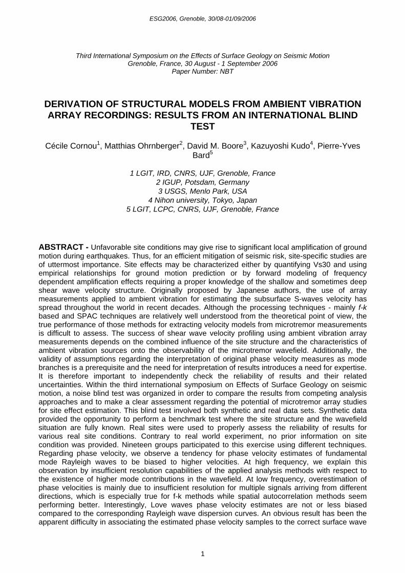
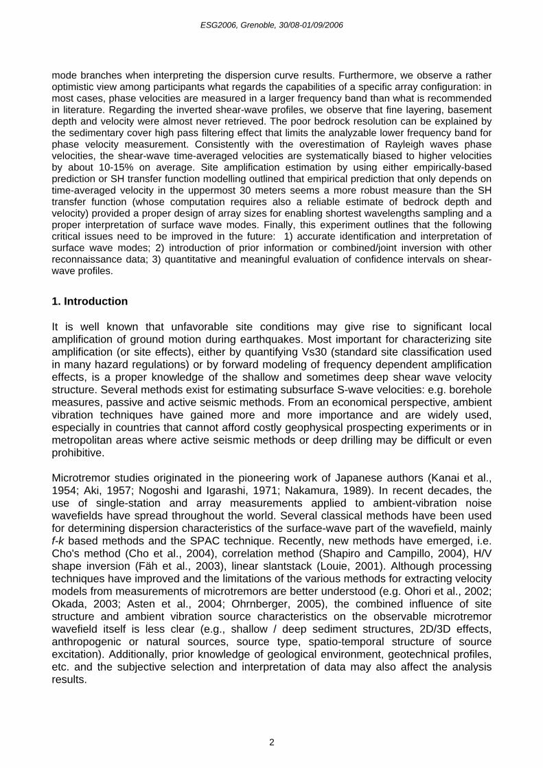
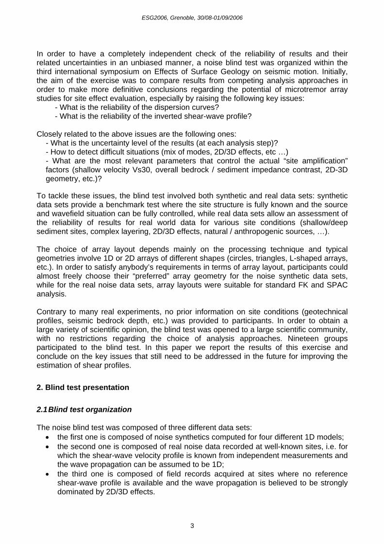
For noise synthetics, one data set consisted of synthetic signals computed at a given array composed of fifteen receivers (Figure 1), while the other three sets consisted of synthetic signals computed at 139 receivers (Figure 2). For the latter data sets, participants were first sent the receivers’ location, one time series recorded at one receiver and the usable frequency band of the noise synthetics considering the applied source time functions. Among these receivers’ locations, participants have then chosen a maximum of three different arrays composed by at most ten receivers each. Hence, for each data set, a total of thirty receivers could be asked for. However, the spatio-temporal source distributions were different for each selected array (individual simulation runs). For real noise data sets, array layouts were naturally fixed. Table 1 lists the different data sets proposed to participants. In order to be able to perform a meaningful overall comparison, the analysis of a minimum number of data sets was requested as indicated in Table 1. Finally, the participants were asked to provide for each data set dispersion curve(s) and shear-wave velocity profile (optionally the compressional-wave one) including, for both estimates, standard deviation.

Figure 1: Array layout for dataset N101.

Figure 2: Location of the 139 receivers proposed for noise synthetics.

Table 1: List of noise data sets

N101 N102 N103 N104 NOISE SYNTHETICS Mandatory

Fixed array layoutMandatory

Free array layout Mandatory

Free array layout Optional

Free array layoutN201 N202 REAL NOISE DATA

Reference Vs profile Mandatory Fixed array layout

Mandatory Fixed array layout

N301 N302 REAL NOISE DATA No reference Vs profile Mandatory

Fixed array layoutOptional

Fixed array layout

ESG2006, Grenoble, 30/08-01/09/2006

5

2.2 Presentation of models Noise synthetics For noise synthetics, the following models were proposed: – a simple gradient (model N101) without interface serving as basic reference; – a complex shallow structure (model N102) with strong impedance contrast and

complex layering including low velocity zones. This model was chosen for verifying the capability of methods to resolve fine layering;

– a deep site (model N103) with strong impedance contrast in order to check the ability of methods to resolve deep layers. The soil profile is very close to the profile of one real site (dataset N201) proposed in this exercise as described in the following section;

– a model involving shallow and deep layers (model N104). Although this model is very simple, its main interest lies in the excitation of higher modes at lower frequency band than fundamental mode.

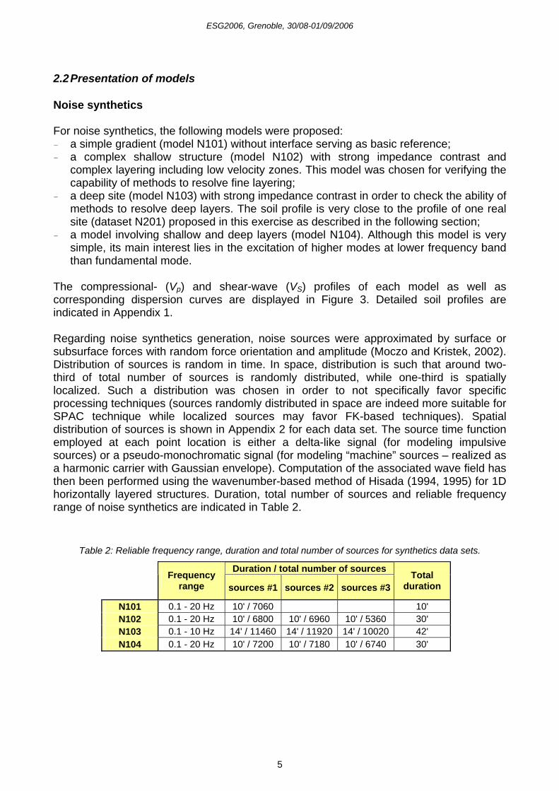
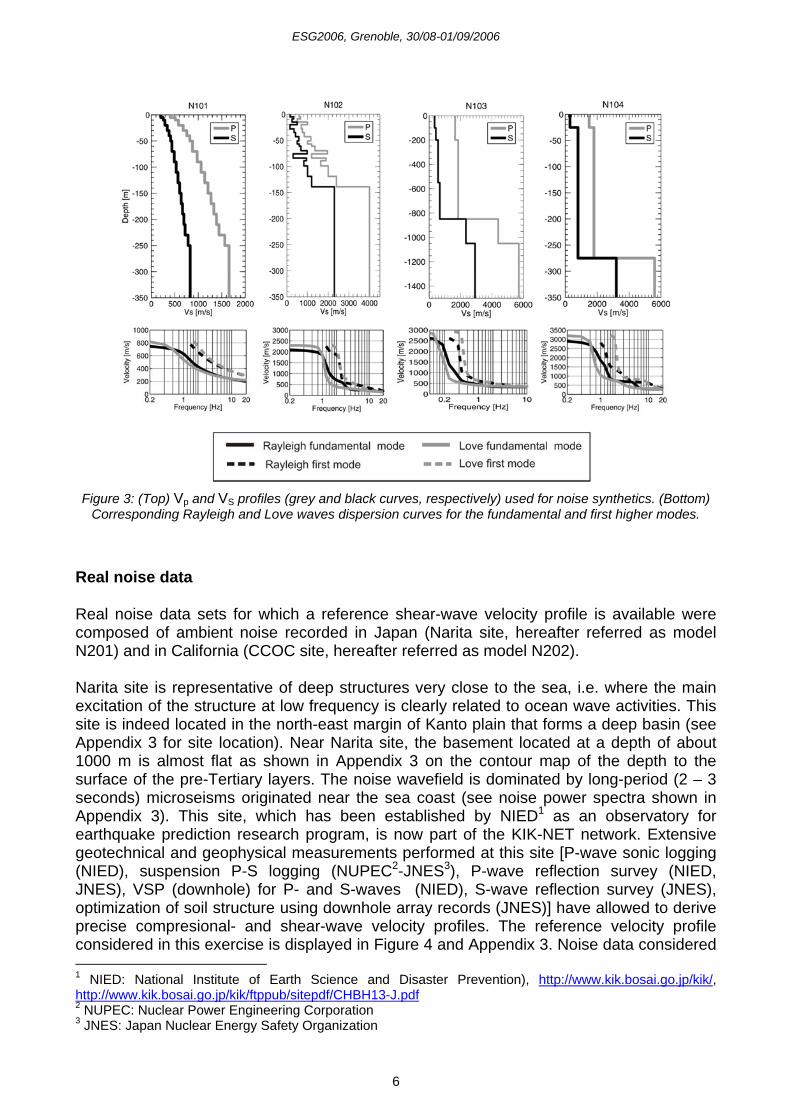
The compressional- (Vp) and shear-wave (VS) profiles of each model as well as corresponding dispersion curves are displayed in Figure 3. Detailed soil profiles are indicated in Appendix 1. Regarding noise synthetics generation, noise sources were approximated by surface or subsurface forces with random force orientation and amplitude (Moczo and Kristek, 2002). Distribution of sources is random in time. In space, distribution is such that around two-third of total number of sources is randomly distributed, while one-third is spatially localized. Such a distribution was chosen in order to not specifically favor specific processing techniques (sources randomly distributed in space are indeed more suitable for SPAC technique while localized sources may favor FK-based techniques). Spatial distribution of sources is shown in Appendix 2 for each data set. The source time function employed at each point location is either a delta-like signal (for modeling impulsive sources) or a pseudo-monochromatic signal (for modeling “machine” sources – realized as a harmonic carrier with Gaussian envelope). Computation of the associated wave field has then been performed using the wavenumber-based method of Hisada (1994, 1995) for 1D horizontally layered structures. Duration, total number of sources and reliable frequency range of noise synthetics are indicated in Table 2.

Table 2: Reliable frequency range, duration and total number of sources for synthetics data sets.

Duration / total number of sources Frequency

range sources #1 sources #2 sources #3Total

duration

N101 0.1 - 20 Hz 10' / 7060 10' N102 0.1 - 20 Hz 10' / 6800 10' / 6960 10' / 5360 30' N103 0.1 - 10 Hz 14' / 11460 14' / 11920 14' / 10020 42' N104 0.1 - 20 Hz 10' / 7200 10' / 7180 10' / 6740 30'

ESG2006, Grenoble, 30/08-01/09/2006

6

Figure 3: (Top) Vp and VS profiles (grey and black curves, respectively) used for noise synthetics. (Bottom)

Corresponding Rayleigh and Love waves dispersion curves for the fundamental and first higher modes.

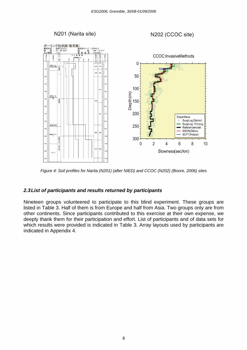
Real noise data Real noise data sets for which a reference shear-wave velocity profile is available were composed of ambient noise recorded in Japan (Narita site, hereafter referred as model N201) and in California (CCOC site, hereafter referred as model N202). Narita site is representative of deep structures very close to the sea, i.e. where the main excitation of the structure at low frequency is clearly related to ocean wave activities. This site is indeed located in the north-east margin of Kanto plain that forms a deep basin (see Appendix 3 for site location). Near Narita site, the basement located at a depth of about 1000 m is almost flat as shown in Appendix 3 on the contour map of the depth to the surface of the pre-Tertiary layers. The noise wavefield is dominated by long-period (2 – 3 seconds) microseisms originated near the sea coast (see noise power spectra shown in Appendix 3). This site, which has been established by NIED1 as an observatory for earthquake prediction research program, is now part of the KIK-NET network. Extensive geotechnical and geophysical measurements performed at this site [P-wave sonic logging (NIED), suspension P-S logging (NUPEC2-JNES3), P-wave reflection survey (NIED, JNES), VSP (downhole) for P- and S-waves (NIED), S-wave reflection survey (JNES), optimization of soil structure using downhole array records (JNES)] have allowed to derive precise compresional- and shear-wave velocity profiles. The reference velocity profile considered in this exercise is displayed in Figure 4 and Appendix 3. Noise data considered 1 NIED: National Institute of Earth Science and Disaster Prevention), http://www.kik.bosai.go.jp/kik/, http://www.kik.bosai.go.jp/kik/ftppub/sitepdf/CHBH13-J.pdf 2 NUPEC: Nuclear Power Engineering Corporation 3 JNES: Japan Nuclear Energy Safety Organization

ESG2006, Grenoble, 30/08-01/09/2006

7

in this exercise were recorded by NUPEC (2002) by using moving-coil type accelerometers (vertical component). The noise data sent to participants were composed of six arrays whose array layouts are displayed in Appendix 3. The CCOC (Coyote Creek Outdoor Classroom) borehole site is located in the Santa Clara valley (see Appendix 3 for site location). The site is underlain by 400 m of flat-lying Quaternary sediments (Wentworth and Tinsley, 2005; see Appendix 3). In situ measurements performed in the borehole (seismic cone penetration testing, surface source-downhole receiver, suspension PS logging) lead to estimate shear-wave velocity profiles within the first 300 meters. The reference shear-wave profile used in this exercise (Figure 4, Appendix 3) was derived from the analysis of several invasive methods (Boore, 2006), and reveals a shallow complex shear-wave velocity layering. Besides, several ambient noise measurements were conducted in the William Street Park (WSP), approximately 200 m far from the Coyote Creek borehole (see Appendix 3), within the framework of a USGS project dedicated to evaluate and compare noninvasive methods for measuring shallow shear-wave velocities in urban areas. Two blind interpretation experiments were indeed conducted at WSP site (Asten and Boore, 2005; Stephenson et al, 2005). Noise data proposed in the present experiment are part of data acquired within this USGS project. Even though ambient noise measurements were not conducted at the borehole site, only little changes in thicknesses and mechanical properties of layers are expected between the CCOC and WSP sites (Wentworth and Tinsley, 2005). Noise data provided to participants were composed of six arrays: for three of them, velocimeters having a cut-off frequency of 0.33 Hz were used (Hartzell et al., 2005), while L4 velocimeters (cut-off frequency of 1 Hz) were used for the other three arrays (Asten, 2005). Array layouts are displayed in Appendix 3. Real noise data sets for which no reference shear-wave profile is available were composed of noise records acquired in the city of Thessaloniki (Greece) (dataset N302) and near Martigny in the Rhône valley (Switzerland) (dataset N301). Although no reference velocity profiles do exist, these sites are interesting since strong 2D/3D wave propagation effects are expected and/or were already observed. In the Rhône valley, Roten et al. (2006) have indeed observed 2D resonances that control the wave propagation at low frequencies, while 2D effects due to a sloping basement interface are expected in Thessaloniki (A. Savaiidis, personal communication). Given the lack of reference velocity profiles and the already substantial length of the present paper, results obtained by participants at those sites will not be discussed. We refer readers to the paper of Roten and Fäh (2006) for more details about the ability of array noise techniques for deriving shear-wave velocities when 2D resonances control the wave propagation.

ESG2006, Grenoble, 30/08-01/09/2006

8

Figure 4: Soil profiles for Narita (N201) (after NIED) and CCOC (N202) (Boore, 2006) sites

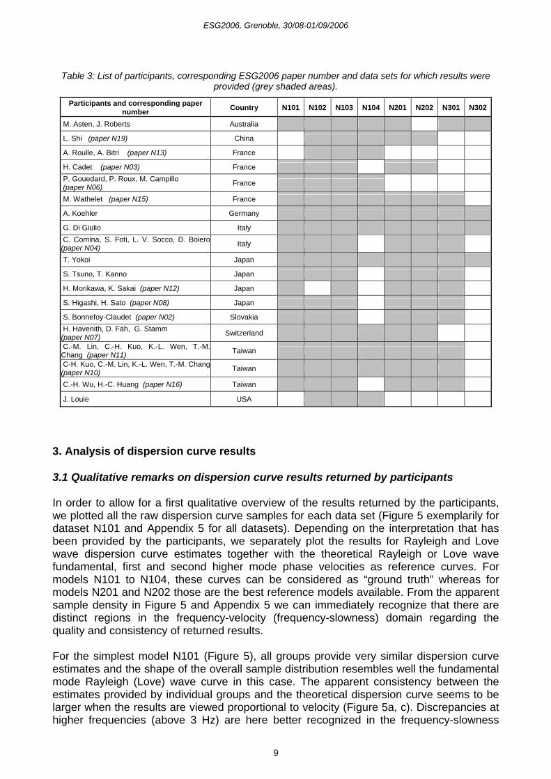
2.3 List of participants and results returned by participants Nineteen groups volunteered to participate to this blind experiment. These groups are listed in Table 3. Half of them is from Europe and half from Asia. Two groups only are from other continents. Since participants contributed to this exercise at their own expense, we deeply thank them for their participation and effort. List of participants and of data sets for which results were provided is indicated in Table 3. Array layouts used by participants are indicated in Appendix 4.

ESG2006, Grenoble, 30/08-01/09/2006

9

Table 3: List of participants, corresponding ESG2006 paper number and data sets for which results were provided (grey shaded areas).

Participants and corresponding paper number Country N101 N102 N103 N104 N201 N202 N301 N302

M. Asten, J. Roberts Australia

L. Shi (paper N19) China

A. Roulle, A. Bitri (paper N13) France

H. Cadet (paper N03) France P. Gouedard, P. Roux, M. Campillo (paper N06) France

M. Wathelet (paper N15) France

A. Koehler Germany

G. Di Giulio Italy C. Comina, S. Foti, L. V. Socco, D. Boiero (paper N04) Italy

T. Yokoi Japan S. Tsuno, T. Kanno Japan

H. Morikawa, K. Sakai (paper N12) Japan

S. Higashi, H. Sato (paper N08) Japan

S. Bonnefoy-Claudet (paper N02) Slovakia H. Havenith, D. Fäh, G. Stamm (paper N07) Switzerland

C.-M. Lin, C.-H. Kuo, K.-L. Wen, T.-M. Chang (paper N11) Taiwan C-H. Kuo, C.-M. Lin, K.-L. Wen, T.-M. Chang (paper N10) Taiwan

C.-H. Wu, H.-C. Huang (paper N16) Taiwan

J. Louie USA

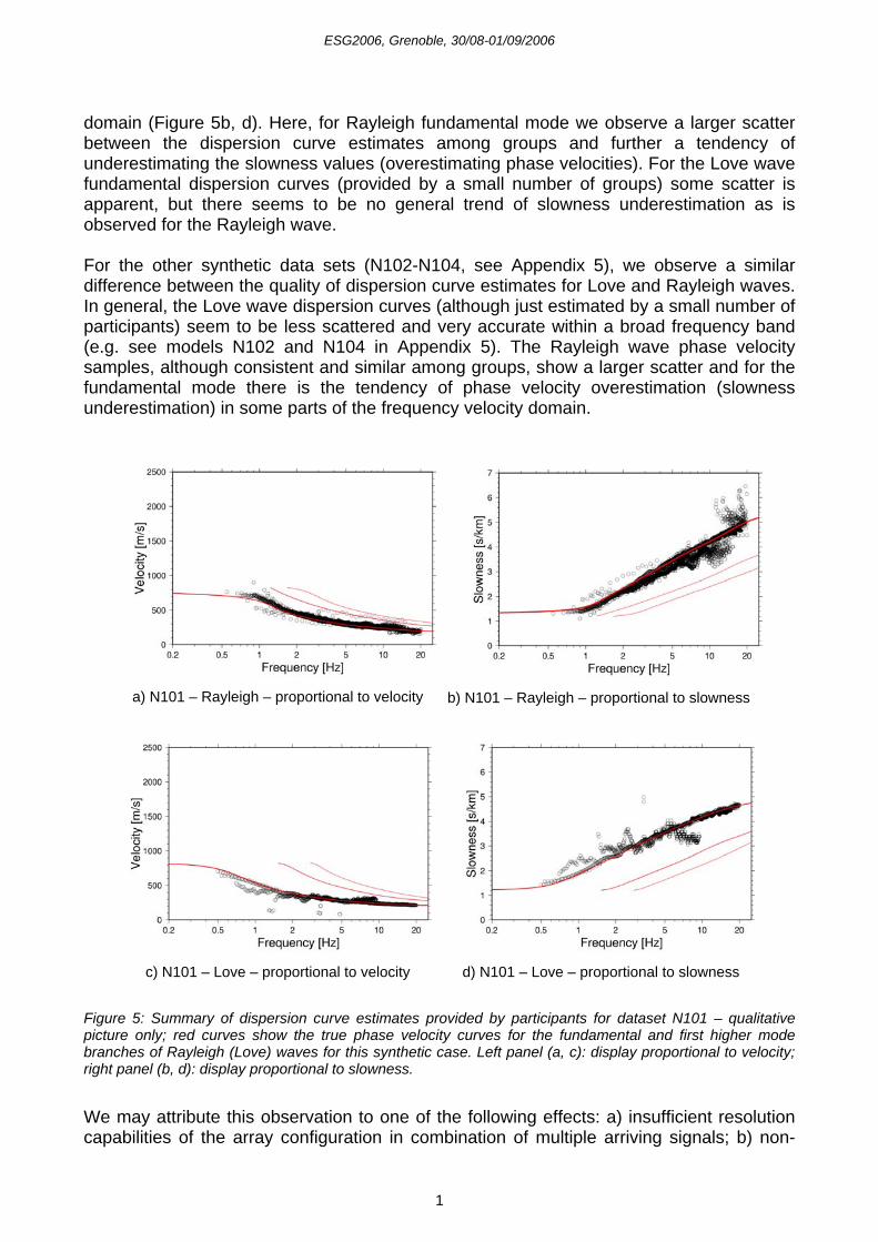
3. Analysis of dispersion curve results 3.1 Qualitative remarks on dispersion curve results returned by participants In order to allow for a first qualitative overview of the results returned by the participants, we plotted all the raw dispersion curve samples for each data set (Figure 5 exemplarily for dataset N101 and Appendix 5 for all datasets). Depending on the interpretation that has been provided by the participants, we separately plot the results for Rayleigh and Love wave dispersion curve estimates together with the theoretical Rayleigh or Love wave fundamental, first and second higher mode phase velocities as reference curves. For models N101 to N104, these curves can be considered as “ground truth” whereas for models N201 and N202 those are the best reference models available. From the apparent sample density in Figure 5 and Appendix 5 we can immediately recognize that there are distinct regions in the frequency-velocity (frequency-slowness) domain regarding the quality and consistency of returned results. For the simplest model N101 (Figure 5), all groups provide very similar dispersion curve estimates and the shape of the overall sample distribution resembles well the fundamental mode Rayleigh (Love) wave curve in this case. The apparent consistency between the estimates provided by individual groups and the theoretical dispersion curve seems to be larger when the results are viewed proportional to velocity (Figure 5a, c). Discrepancies at higher frequencies (above 3 Hz) are here better recognized in the frequency-slowness

ESG2006, Grenoble, 30/08-01/09/2006

1

domain (Figure 5b, d). Here, for Rayleigh fundamental mode we observe a larger scatter between the dispersion curve estimates among groups and further a tendency of underestimating the slowness values (overestimating phase velocities). For the Love wave fundamental dispersion curves (provided by a small number of groups) some scatter is apparent, but there seems to be no general trend of slowness underestimation as is observed for the Rayleigh wave. For the other synthetic data sets (N102-N104, see Appendix 5), we observe a similar difference between the quality of dispersion curve estimates for Love and Rayleigh waves. In general, the Love wave dispersion curves (although just estimated by a small number of participants) seem to be less scattered and very accurate within a broad frequency band (e.g. see models N102 and N104 in Appendix 5). The Rayleigh wave phase velocity samples, although consistent and similar among groups, show a larger scatter and for the fundamental mode there is the tendency of phase velocity overestimation (slowness underestimation) in some parts of the frequency velocity domain.

a) N101 – Rayleigh – proportional to velocity b) N101 – Rayleigh – proportional to slowness

c) N101 – Love – proportional to velocity d) N101 – Love – proportional to slowness Figure 5: Summary of dispersion curve estimates provided by participants for dataset N101 – qualitative picture only; red curves show the true phase velocity curves for the fundamental and first higher mode branches of Rayleigh (Love) waves for this synthetic case. Left panel (a, c): display proportional to velocity; right panel (b, d): display proportional to slowness.

We may attribute this observation to one of the following effects: a) insufficient resolution capabilities of the array configuration in combination of multiple arriving signals; b) non-

ESG2006, Grenoble, 30/08-01/09/2006

1

plane wave arrivals. For case a) there are two further effects to distinguish: i) multiple signals may be arriving from distinct directions but travelling at the same wavenumber; ii) multiple signals may be arriving from the same direction but travelling at distinct wavenumbers. The situation described in a.i) is problematic for frequency-wavenumber estimation techniques in the longer wavelength range, where the resolution capabilities are insufficient to separate individual signals from distinct directions. Then, the superposition of array response functions for all arriving signals leads to a biased velocity estimate. The resulting velocities are too high compared to the true propagation velocities (see e.g. Ohrnberger et al., 2004). The same wavefield situation, however, should pose no major difficulty for spatial autocorrelation techniques which are specifically developed for this wavefield scenario (random stationary wavefield). Situation a.ii) corresponds to the existence of a non-negligible contribution of higher mode waves in the wavefield. It has been noted earlier (Tokimatsu et al., 1992a, 1992b; Tokimatsu, 1997, Rix and Lai, 1998) that for wavefields composed of multiple modes with similar energy contribution the phase velocity values obtained from array analysis are no longer providing estimates for individual mode branches but rather represent intermediate phase velocities between the interacting modes. This observation is a result of insufficient resolution capabilities of the applied array analysis method related to one of the following causes. Bias as a result of insufficient resolution may e.g. be due to the violation of underlying assumptions for a certain method. The classical SPAC method as described by Aki (1957), for example, is based on the assumption of a single valued wavenumber component per frequency contained in the wavefield, i.e. whenever there are higher modes present in the wavefield, the resulting autocorrelation value will relate to the superposed modes rather than to individual ones. For f-k techniques on the other hand, the success in separating the individual mode branches depends on the wavelengths to be analysed related to the resolution capabilities of the array geometry (e.g. Socco and Strobbia, 2004). An additional underlying assumption for applying any array analysis method is that the observed signals are completely uncorrelated and propagating as plane waves. Correlated signals are known to reduce significantly the performance of any frequency wavenumber based array technique (Woods and Lintz, 1973, Krim and Viberg, 1996; Cornou et al., 2003; Schissele et al., 2004). In the case of ambient vibration, we expect that multiple mode signals are generated by one and the same source, hence being strongly correlated and therefore representing an unfavourable condition for any method of being able to resolve individual mode branches in the wavefield. Situation b), the arrival of non-plane waves, violating a fundamental assumption on which array techniques are based on, can be related either to lateral heterogeneities of the medium producing undulated wavefronts (a scattered wavefield in general) or to the existence of close sources to the array setting leading to curved wavefronts (see e.g. Almendros et al., 1999; Ohrnberger et al., 2004). Considering the source distributions in the synthetic data sets N101 to N104, close point sources are existent and the contribution of this non-plane wavefield portion varies in dependence of the chosen array layout from small to large apertures. The overestimation of phase velocity for the synthetic data set N101 (Figure 5) is observed for the fundamental Rayleigh mode, but not for the fundamental Love wave dispersion curves. The most likely cause for this velocity overestimation according to this observation

ESG2006, Grenoble, 30/08-01/09/2006

1

is the existence of higher mode contributions of Rayleigh waves in combination with insufficient resolution capabilities of the applied array methods.

a) N102 – Rayleigh fundamental interpretation b) N102 – Rayleigh 1st higher mode interpretation

c) N104 – Rayleigh fundamental interpretation d) N104 – Rayleigh 1st higher mode interpretation

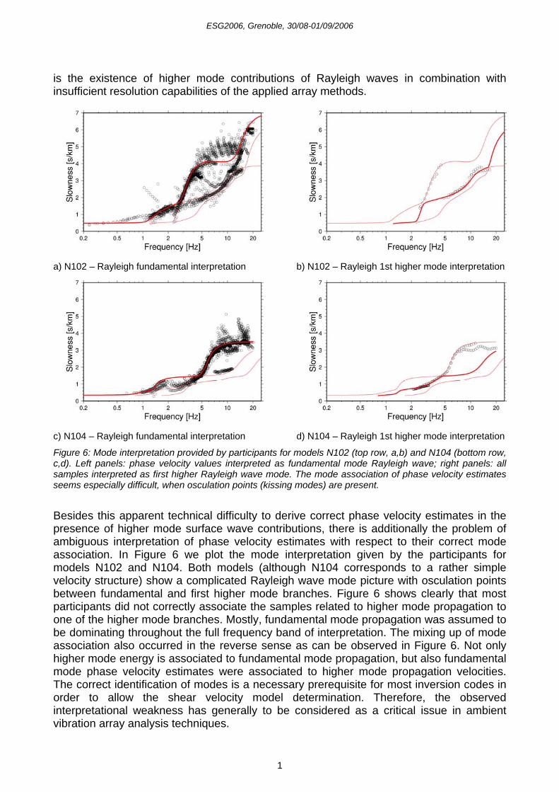
Figure 6: Mode interpretation provided by participants for models N102 (top row, a,b) and N104 (bottom row, c,d). Left panels: phase velocity values interpreted as fundamental mode Rayleigh wave; right panels: all samples interpreted as first higher Rayleigh wave mode. The mode association of phase velocity estimates seems especially difficult, when osculation points (kissing modes) are present.

Besides this apparent technical difficulty to derive correct phase velocity estimates in the presence of higher mode surface wave contributions, there is additionally the problem of ambiguous interpretation of phase velocity estimates with respect to their correct mode association. In Figure 6 we plot the mode interpretation given by the participants for models N102 and N104. Both models (although N104 corresponds to a rather simple velocity structure) show a complicated Rayleigh wave mode picture with osculation points between fundamental and first higher mode branches. Figure 6 shows clearly that most participants did not correctly associate the samples related to higher mode propagation to one of the higher mode branches. Mostly, fundamental mode propagation was assumed to be dominating throughout the full frequency band of interpretation. The mixing up of mode association also occurred in the reverse sense as can be observed in Figure 6. Not only higher mode energy is associated to fundamental mode propagation, but also fundamental mode phase velocity estimates were associated to higher mode propagation velocities. The correct identification of modes is a necessary prerequisite for most inversion codes in order to allow the shear velocity model determination. Therefore, the observed interpretational weakness has generally to be considered as a critical issue in ambient vibration array analysis techniques.

ESG2006, Grenoble, 30/08-01/09/2006

1

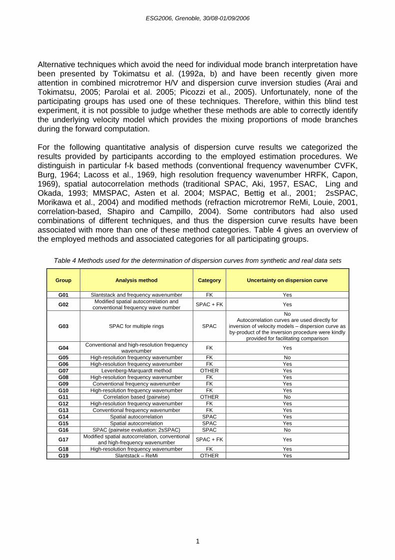
Alternative techniques which avoid the need for individual mode branch interpretation have been presented by Tokimatsu et al. (1992a, b) and have been recently given more attention in combined microtremor H/V and dispersion curve inversion studies (Arai and Tokimatsu, 2005; Parolai et al. 2005; Picozzi et al., 2005). Unfortunately, none of the participating groups has used one of these techniques. Therefore, within this blind test experiment, it is not possible to judge whether these methods are able to correctly identify the underlying velocity model which provides the mixing proportions of mode branches during the forward computation. For the following quantitative analysis of dispersion curve results we categorized the results provided by participants according to the employed estimation procedures. We distinguish in particular f-k based methods (conventional frequency wavenumber CVFK, Burg, 1964; Lacoss et al., 1969, high resolution frequency wavenumber HRFK, Capon, 1969), spatial autocorrelation methods (traditional SPAC, Aki, 1957, ESAC, Ling and Okada, 1993; MMSPAC, Asten et al. 2004; MSPAC, Bettig et al., 2001; 2sSPAC, Morikawa et al., 2004) and modified methods (refraction microtremor ReMi, Louie, 2001, correlation-based, Shapiro and Campillo, 2004). Some contributors had also used combinations of different techniques, and thus the dispersion curve results have been associated with more than one of these method categories. Table 4 gives an overview of the employed methods and associated categories for all participating groups.

Table 4 Methods used for the determination of dispersion curves from synthetic and real data sets

Group Analysis method Category Uncertainty on dispersion curve

G01 Slantstack and frequency wavenumber FK Yes

G02 Modified spatial autocorrelation and conventional frequency wave number SPAC + FK Yes

G03 SPAC for multiple rings SPAC

No Autocorrelation curves are used directly for

inversion of velocity models – dispersion curve as by-product of the inversion procedure were kindly

provided for facilitating comparison

G04 Conventional and high-resolution frequency wavenumber FK Yes

G05 High-resolution frequency wavenumber FK No G06 High-resolution frequency wavenumber FK Yes G07 Levenberg-Marquardt method OTHER Yes G08 High-resolution frequency wavenumber FK Yes G09 Conventional frequency wavenumber FK Yes G10 High-resolution frequency wavenumber FK Yes G11 Correlation based (pairwise) OTHER No G12 High-resolution frequency wavenumber FK Yes G13 Conventional frequency wavenumber FK Yes G14 Spatial autocorrelation SPAC Yes G15 Spatial autocorrelation SPAC Yes G16 SPAC (pairwise evaluation: 2sSPAC) SPAC No

G17 Modified spatial autocorrelation, conventional and high-frequency wavenumber SPAC + FK Yes

G18 High-resolution frequency wavenumber FK Yes G19 Slantstack – ReMi OTHER Yes

ESG2006, Grenoble, 30/08-01/09/2006

1

3.2 Quantitative misfit computation of dispersion curve estimates – an attempt for a fair comparison of results obtained with distinct array geometries According to the rules of this blind prediction experiment, the participants were allowed to choose individual array layouts for each of the synthetic data sets N102, N103 and N104 (see Table 1). In order to facilitate the quantitative comparison of phase velocity curves estimated for these data sets, we need to take into account the resolution capabilities of the array geometries which have been used for the estimation procedure. We have followed here a simple strategy to accomplish a quantitative comparison of results. Any seismic array configuration can be considered as a discrete spatial sampling process of the continuous seismic wavefield in space and time. As a consequence, the sampling theorem holds and the short-wavelength part of the wavefield cannot be recovered uniquely (spatial aliasing). For 1-dimensional equidistantly spaced sensor networks, the relation between the interstation distance d of neighboring stations and the spatial Nyquist frequency λNyq can be specified simply by the requirement that each wavelength needs to be sampled (equidistantly) by at least two discrete sampling positions:

λNyq = λmin = 2d (1) On the opposite end of the wavelength interval, another limitation exists. The resolution capability of a seismic array configuration, that is the capability to separate two waves propagating at closely spaced wavenumbers, is related to the maximum interstation distance D, the so-called aperture of the array:

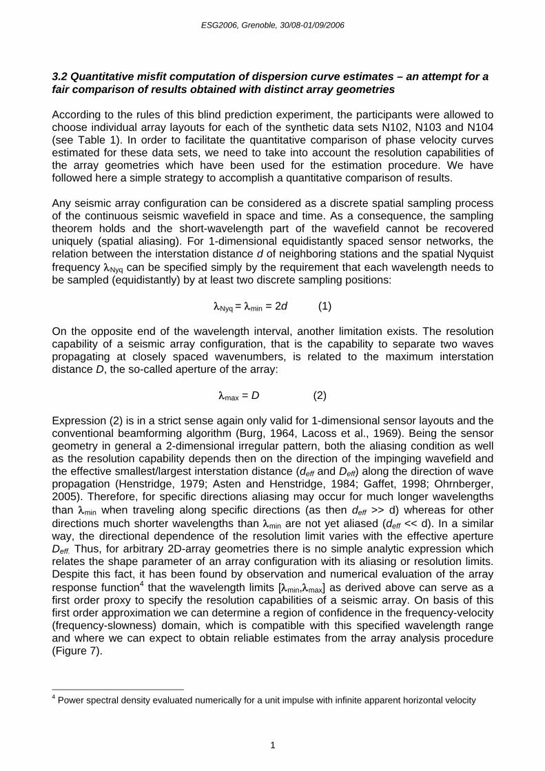
λmax = D (2) Expression (2) is in a strict sense again only valid for 1-dimensional sensor layouts and the conventional beamforming algorithm (Burg, 1964, Lacoss et al., 1969). Being the sensor geometry in general a 2-dimensional irregular pattern, both the aliasing condition as well as the resolution capability depends then on the direction of the impinging wavefield and the effective smallest/largest interstation distance (deff and Deff) along the direction of wave propagation (Henstridge, 1979; Asten and Henstridge, 1984; Gaffet, 1998; Ohrnberger, 2005). Therefore, for specific directions aliasing may occur for much longer wavelengths than λmin when traveling along specific directions (as then deff >> d) whereas for other directions much shorter wavelengths than λmin are not yet aliased (deff << d). In a similar way, the directional dependence of the resolution limit varies with the effective aperture Deff. Thus, for arbitrary 2D-array geometries there is no simple analytic expression which relates the shape parameter of an array configuration with its aliasing or resolution limits. Despite this fact, it has been found by observation and numerical evaluation of the array response function4 that the wavelength limits [λmin,λmax] as derived above can serve as a first order proxy to specify the resolution capabilities of a seismic array. On basis of this first order approximation we can determine a region of confidence in the frequency-velocity (frequency-slowness) domain, which is compatible with this specified wavelength range and where we can expect to obtain reliable estimates from the array analysis procedure (Figure 7). 4 Power spectral density evaluated numerically for a unit impulse with infinite apparent horizontal velocity

ESG2006, Grenoble, 30/08-01/09/2006

1

Figure 7: Determination of reliable region for quantitative dispersion curve interpretation from basic array geometry properties (d = minimum inter-station distance, D = aperture, maximum inter-station distance).

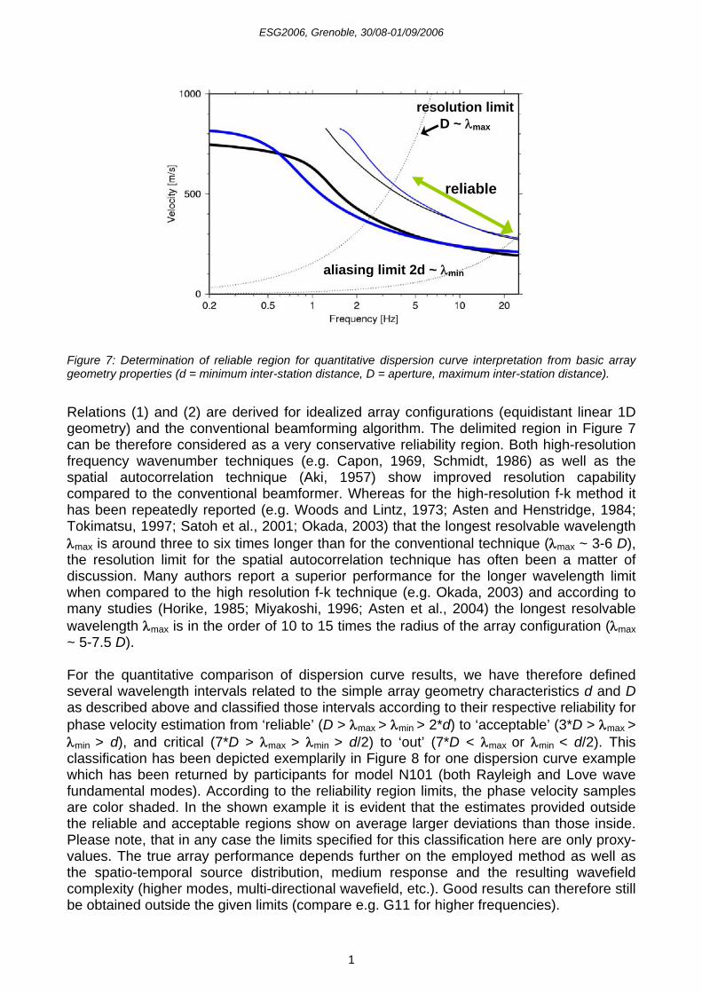
Relations (1) and (2) are derived for idealized array configurations (equidistant linear 1D geometry) and the conventional beamforming algorithm. The delimited region in Figure 7 can be therefore considered as a very conservative reliability region. Both high-resolution frequency wavenumber techniques (e.g. Capon, 1969, Schmidt, 1986) as well as the spatial autocorrelation technique (Aki, 1957) show improved resolution capability compared to the conventional beamformer. Whereas for the high-resolution f-k method it has been repeatedly reported (e.g. Woods and Lintz, 1973; Asten and Henstridge, 1984; Tokimatsu, 1997; Satoh et al., 2001; Okada, 2003) that the longest resolvable wavelength λmax is around three to six times longer than for the conventional technique (λmax ~ 3-6 D), the resolution limit for the spatial autocorrelation technique has often been a matter of discussion. Many authors report a superior performance for the longer wavelength limit when compared to the high resolution f-k technique (e.g. Okada, 2003) and according to many studies (Horike, 1985; Miyakoshi, 1996; Asten et al., 2004) the longest resolvable wavelength λmax is in the order of 10 to 15 times the radius of the array configuration (λmax ~ 5-7.5 D). For the quantitative comparison of dispersion curve results, we have therefore defined several wavelength intervals related to the simple array geometry characteristics d and D as described above and classified those intervals according to their respective reliability for phase velocity estimation from ‘reliable’ (D > λmax > λmin > 2*d) to ‘acceptable’ (3*D > λmax > λmin > d), and critical (7*D > λmax > λmin > d/2) to ‘out’ (7*D < λmax or λmin < d/2). This classification has been depicted exemplarily in Figure 8 for one dispersion curve example which has been returned by participants for model N101 (both Rayleigh and Love wave fundamental modes). According to the reliability region limits, the phase velocity samples are color shaded. In the shown example it is evident that the estimates provided outside the reliable and acceptable regions show on average larger deviations than those inside. Please note, that in any case the limits specified for this classification here are only proxy-values. The true array performance depends further on the employed method as well as the spatio-temporal source distribution, medium response and the resulting wavefield complexity (higher modes, multi-directional wavefield, etc.). Good results can therefore still be obtained outside the given limits (compare e.g. G11 for higher frequencies).

aliasing limit 2d ~ λmin

reliable

resolution limit D ~ λmax

ESG2006, Grenoble, 30/08-01/09/2006

1

Figure 8: Dispersion curve estimates are shown in color according to the reliability regions determined from the array geometry which has been used for estimating the phase velocities. Intensive green symbols show values falling inside the reliable region. Faded green symbols are used for the acceptable frequency-velocity ranges, faded red symbols for the critical range and intensive red for values outside the most optimistic wavelength limits.

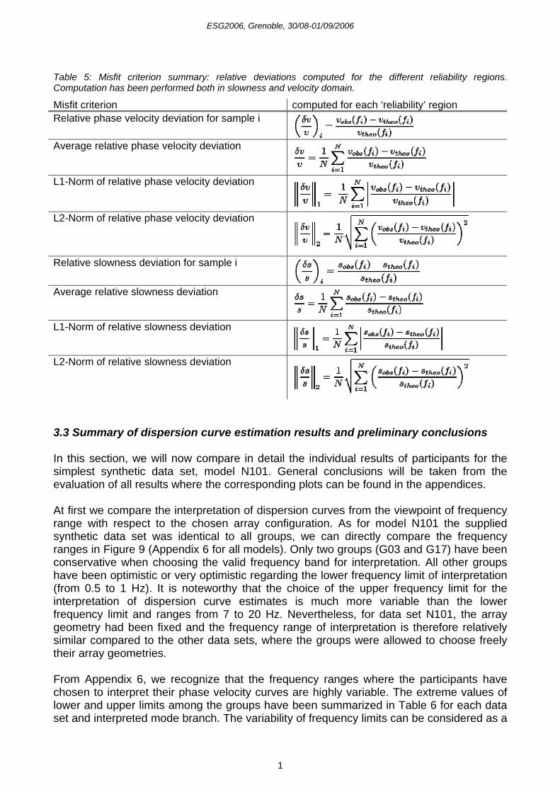
In order to assess the estimation performance of dispersion curves by the individual groups and/or applied methods, we compute then a quantitative misfit of the dispersion curve estimates separately for the different ‘reliability‘-regions and compare these misfit values between individual groups. As misfit quantity, we have computed both absolute and relative deviations between each phase velocity sample and its corresponding reference value (theoretical curves) according to the mode interpretation given by each group. In the following, we will refer only to the relative deviations as given in Table 5 as we consider these quantities to provide the most relevant information for the comparison between dispersion curve estimates. Note that from the viewpoint of error propagation in the estimation technique it is favorable to compute the misfit quantities proportional to slowness (see Boore and Brown, 1998 for a detailed discussion). In this study we have though decided to compute both deviations proportional to slowness as well as proportional to velocity. The velocity deviations are provided for convenience and in accordance with the preference of the engineering community.

ESG2006, Grenoble, 30/08-01/09/2006

1

Table 5: Misfit criterion summary: relative deviations computed for the different reliability regions. Computation has been performed both in slowness and velocity domain.

Misfit criterion computed for each ‘reliability’ region Relative phase velocity deviation for sample i

Average relative phase velocity deviation

L1-Norm of relative phase velocity deviation

L2-Norm of relative phase velocity deviation

Relative slowness deviation for sample i

Average relative slowness deviation

L1-Norm of relative slowness deviation

L2-Norm of relative slowness deviation

3.3 Summary of dispersion curve estimation results and preliminary conclusions In this section, we will now compare in detail the individual results of participants for the simplest synthetic data set, model N101. General conclusions will be taken from the evaluation of all results where the corresponding plots can be found in the appendices. At first we compare the interpretation of dispersion curves from the viewpoint of frequency range with respect to the chosen array configuration. As for model N101 the supplied synthetic data set was identical to all groups, we can directly compare the frequency ranges in Figure 9 (Appendix 6 for all models). Only two groups (G03 and G17) have been conservative when choosing the valid frequency band for interpretation. All other groups have been optimistic or very optimistic regarding the lower frequency limit of interpretation (from 0.5 to 1 Hz). It is noteworthy that the choice of the upper frequency limit for the interpretation of dispersion curve estimates is much more variable than the lower frequency limit and ranges from 7 to 20 Hz. Nevertheless, for data set N101, the array geometry had been fixed and the frequency range of interpretation is therefore relatively similar compared to the other data sets, where the groups were allowed to choose freely their array geometries. From Appendix 6, we recognize that the frequency ranges where the participants have chosen to interpret their phase velocity curves are highly variable. The extreme values of lower and upper limits among the groups have been summarized in Table 6 for each data set and interpreted mode branch. The variability of frequency limits can be considered as a

ESG2006, Grenoble, 30/08-01/09/2006

1

clear indication that the proper design of array sizes and corresponding interpretation of dispersion curve is a difficult matter whenever no prior information about a site is available.

Figure 9: Direct comparison of interpreted frequency ranges by individual groups for model N101. The horizontal bars cover the entire frequency band within which phase velocity estimates have been provided by the participants (small numbers to the right specify the mode number: 0: fundamental, 1: 1st higher). Color shading corresponds to the individual reliability regions as introduced in Figure 8. For model N101 all groups used the same data from the fixed array geometry. Therefore, the differences in the frequency range correspond directly to the individual interpretation of dispersion curve estimate validity by the groups. Figures for other models can be found in Appendix 6.

Table 6: Summary of frequency limits for individual surface wave mode branches (R: Rayleigh; L: Love; 00: fundamental mode; 01 first higher mode; 02: second higher mode) as evaluated by participants. The ranges

for the lower and upper frequency limits are given in Hz.

Model N101 N102 N103 N104 N201 N202 lower

f-limit upper f-limit

lower f-limit

upper f-limit

lowerf-limit

upper f-limit

lowerf-limit

upper f-limit

lower f-limit

upper f-limit

lowerf-limit

upper f-limit

R00 0.55-3.24

7.50-20.00

0.23-2.91

2.05-21.60

0.13-1.60

1.02-10.20

0.65-7.00

1.80-20.20

0.15-1.95

0.44-13.00

0.24-1.30

1.66-20.00

R01 3.00 15.00 2.50-5.55

4.45-16.91

- - 2.10-2.75

3.20-20.00

8.08 12.00 3.40 3.90

R02 - - 6.55 12.71 - - - - - - 3.50 5.10 L00 0.50-

1.75 6.52-19.94

1.02-1.30

11.68-20.00

0.18-0.40

1.86-6.95

0.70-0.90

14.00-17.94

- - 0.95 1.00

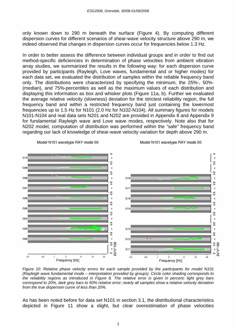
When displaying the sample-wise relative velocity misfit for model N101 in Figure 10 (fundamental mode Rayleigh wave estimates), we observe that almost all individual velocity deviations are less than 20% of the true value. As expected, the largest misfits are observed at frequencies where the wavelength criteria for the reliable and acceptable regions of the frequency velocity domain are not met. All detailed displays of sample-wise relative deviations are summarized in Appendix 7 for all models (Rayleigh fundamental wave only). For N202 model, our computation of the relative misfit is most probably erroneous within the lowest frequency band (below 1.3 Hz) since the reference profile is

ESG2006, Grenoble, 30/08-01/09/2006

1

only known down to 290 m beneath the surface (Figure 4). By computing different dispersion curves for different scenarios of shear-wave velocity structure above 290 m, we indeed observed that changes in dispersion curves occur for frequencies below 1.3 Hz. In order to better assess the difference between individual groups and in order to find out method-specific deficiencies in determination of phase velocities from ambient vibration array studies, we summarized the results in the following way: for each dispersion curve provided by participants (Rayleigh, Love waves, fundamental and or higher modes) for each data set, we evaluated the distribution of samples within the reliable frequency band only. The distributions were characterized by specifying the minimum, the 25%-, 50%- (median), and 75%-percentiles as well as the maximum values of each distribution and displaying this information as box and whisker plots (Figure 11a, b). Further we evaluated the average relative velocity (slowness) deviation for the strictest reliability region, the full frequency band and within a restricted frequency band just containing the lowermost frequencies up to 1.5 Hz for N101 (2.0 Hz for N102-N104). All summary figures for models N101-N104 and real data sets N201 and N202 are provided in Appendix 8 and Appendix 9 for fundamental Rayleigh wave and Love wave modes, respectively. Note also that for N202 model, computation of distribution was performed within the “safe” frequency band regarding our lack of knowledge of shear-wave velocity variation for depth above 290 m.

Figure 10: Relative phase velocity errors for each sample provided by the participants for model N101 (Rayleigh wave fundamental mode – interpretation provided by groups). Circle color shading corresponds to the reliability regions as introduced in Figure 8. The relative error is given in percent; light grey bars correspond to 20%, dark grey bars to 50% relative error; nearly all samples show a relative velocity deviation from the true dispersion curve of less than 20%.

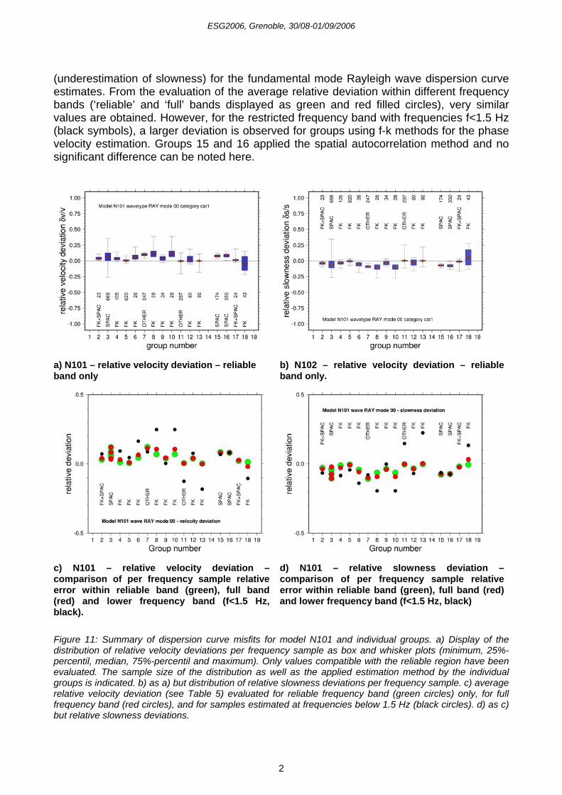
As has been noted before for data set N101 in section 3.1, the distributional characteristics depicted in Figure 11 show a slight, but clear overestimation of phase velocities

ESG2006, Grenoble, 30/08-01/09/2006

2

(underestimation of slowness) for the fundamental mode Rayleigh wave dispersion curve estimates. From the evaluation of the average relative deviation within different frequency bands (‘reliable’ and ‘full’ bands displayed as green and red filled circles), very similar values are obtained. However, for the restricted frequency band with frequencies f<1.5 Hz (black symbols), a larger deviation is observed for groups using f-k methods for the phase velocity estimation. Groups 15 and 16 applied the spatial autocorrelation method and no significant difference can be noted here.

a) N101 – relative velocity deviation – reliable band only

b) N102 – relative velocity deviation – reliable band only.

c) N101 – relative velocity deviation – comparison of per frequency sample relative error within reliable band (green), full band (red) and lower frequency band (f<1.5 Hz, black).

d) N101 – relative slowness deviation – comparison of per frequency sample relative error within reliable band (green), full band (red) and lower frequency band (f<1.5 Hz, black)

Figure 11: Summary of dispersion curve misfits for model N101 and individual groups. a) Display of the distribution of relative velocity deviations per frequency sample as box and whisker plots (minimum, 25%-percentil, median, 75%-percentil and maximum). Only values compatible with the reliable region have been evaluated. The sample size of the distribution as well as the applied estimation method by the individual groups is indicated. b) as a) but distribution of relative slowness deviations per frequency sample. c) average relative velocity deviation (see Table 5) evaluated for reliable frequency band (green circles) only, for full frequency band (red circles), and for samples estimated at frequencies below 1.5 Hz (black circles). d) as c) but relative slowness deviations.

ESG2006, Grenoble, 30/08-01/09/2006

2

Due to the wrong association of phase velocity samples to the individual modes, the same evaluation for models N102 and N104, where strong higher mode contribution is present, does not lead to an easy conclusion. For model N103, however, we can observe again larger deviations for f-k based methods. Similar to model N101, we can also again confirm the slight overestimation of phase velocities. A much stronger deviation of relative phase velocity deviations are observed for the real data sets N201 and N202. The median values of the sample distributions returned by the participants range from +20% to +80% when evaluated in terms of phase velocity and -15% to -60% when evaluated in terms of slowness for data set N201. For data set N202 we obtain slightly better values ranging from +5% to +75% in velocity deviation and -5% to -50% in slowness. This strong bias of estimated dispersion curve values is surprising as the real sites N201 and N202 correspond in complexity and shape of velocity model to the synthetic case models N103 and N102, for which the dispersion curve values have been much better retrieved. So far, we have no specific explanation for this observation. One possible - but also disturbing - answer is related to the question of the reference soil profiles used for sites N201 and N202 and whether those represent the observed ambient vibration data. Even though Love wave fundamental dispersion curves have been provided by only a small number of participants, we can observe that the median values of the relative phase velocity deviations are less than 10% for models N101-N104.

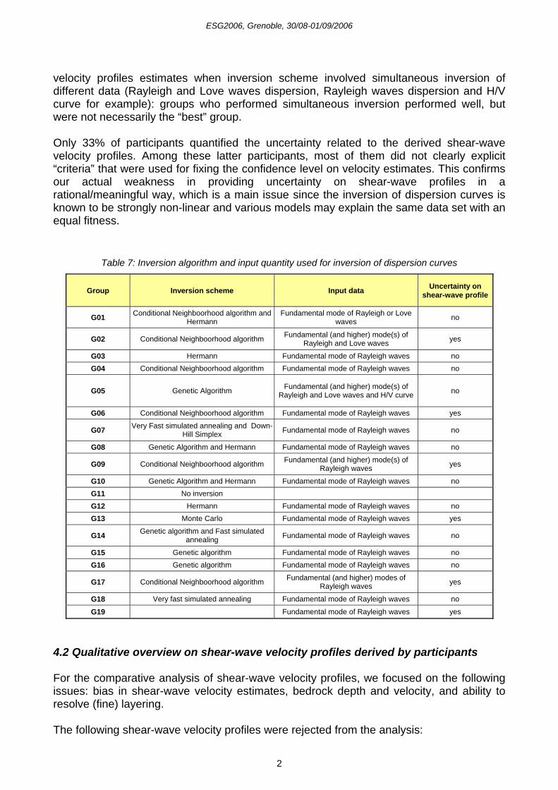
4. Analysis of velocity profile results 4.1 Overview of the methods used by participants Table 7 lists the different methods and the input data (fundamental mode of Rayleigh and/or Love waves, fundamental and higher modes, H/V spectral ratio) used by participants for inverting the dispersion curves. Participants have used one or more of the following methods: direct search methods that generate random models into a bounded parameter space like Neighborhood Algorithm (Sambridge, 1999; Wathelet et al., 2004, 2005), Genetic Algorithm (Goldberg, 1989; Stoffa and Sen 1991; Lomax and Snieder, 1994; Boschetti et al., 1996; Yamanaka and Ishida, 1996), Simulated Annealing (Rothman 1985; Sen and Stoffa1991), Monte Carlo algorithm (Edwards, 1992; Mosegaard and Tarantola,1995) or linearized and iterative optimization methods (Herrmann, 1987). In addition to this variety of inversion schemes, data to be inverted were varying from participant to participant: some inverted the fundamental mode of Rayleigh waves only, some simultaneously inverted the Rayleigh and Love fundamental wave modes, some simultaneously inverted fundamental and higher modes, and finally some also included the inversion of H/V ratios. Finally, it appeared that there were as many different inversion schemes as the number of participants. It was thus rather difficult - and even impossible - to perform a fair and quantitative comparison of the different inversion approaches. In the following sections, we will therefore only focus on the analysis of final shear-velocity profiles and disregard comparative performance of the different inversion schemes. However, it has to be pointed out that no clear improvement in shear-wave velocity profiles could be noticed regarding the type of data inverted by participants. Although the number of participating groups is too small to conclude statistically on the results, we could not observe clear improvement in

ESG2006, Grenoble, 30/08-01/09/2006

2

velocity profiles estimates when inversion scheme involved simultaneous inversion of different data (Rayleigh and Love waves dispersion, Rayleigh waves dispersion and H/V curve for example): groups who performed simultaneous inversion performed well, but were not necessarily the “best” group. Only 33% of participants quantified the uncertainty related to the derived shear-wave velocity profiles. Among these latter participants, most of them did not clearly explicit “criteria” that were used for fixing the confidence level on velocity estimates. This confirms our actual weakness in providing uncertainty on shear-wave profiles in a rational/meaningful way, which is a main issue since the inversion of dispersion curves is known to be strongly non-linear and various models may explain the same data set with an equal fitness.

Table 7: Inversion algorithm and input quantity used for inversion of dispersion curves

Group Inversion scheme Input data Uncertainty on shear-wave profile

G01 Conditional Neighboorhood algorithm and Hermann

Fundamental mode of Rayleigh or Love waves no

G02 Conditional Neighboorhood algorithm Fundamental (and higher) mode(s) of Rayleigh and Love waves yes

G03 Hermann Fundamental mode of Rayleigh waves no

G04 Conditional Neighboorhood algorithm Fundamental mode of Rayleigh waves no

G05 Genetic Algorithm Fundamental (and higher) mode(s) of Rayleigh and Love waves and H/V curve no

G06 Conditional Neighboorhood algorithm Fundamental mode of Rayleigh waves yes

G07 Very Fast simulated annealing and Down-Hill Simplex Fundamental mode of Rayleigh waves no

G08 Genetic Algorithm and Hermann Fundamental mode of Rayleigh waves no

G09 Conditional Neighboorhood algorithm Fundamental (and higher) mode(s) of Rayleigh waves yes

G10 Genetic Algorithm and Hermann Fundamental mode of Rayleigh waves no

G11 No inversion

G12 Hermann Fundamental mode of Rayleigh waves no

G13 Monte Carlo Fundamental mode of Rayleigh waves yes

G14 Genetic algorithm and Fast simulated annealing Fundamental mode of Rayleigh waves no

G15 Genetic algorithm Fundamental mode of Rayleigh waves no

G16 Genetic algorithm Fundamental mode of Rayleigh waves no

G17 Conditional Neighboorhood algorithm Fundamental (and higher) modes of Rayleigh waves yes

G18 Very fast simulated annealing Fundamental mode of Rayleigh waves no

G19 Fundamental mode of Rayleigh waves yes

4.2 Qualitative overview on shear-wave velocity profiles derived by participants For the comparative analysis of shear-wave velocity profiles, we focused on the following issues: bias in shear-wave velocity estimates, bedrock depth and velocity, and ability to resolve (fine) layering. The following shear-wave velocity profiles were rejected from the analysis:

ESG2006, Grenoble, 30/08-01/09/2006

2

- Shear-wave velocity profiles derived by using incorrect interpretation of surface wave modes;

- Shear-wave velocity profiles derived by using very erroneous phase velocity measurement;

- Shear-wave velocity profiles derived by inverting separately dispersion curves obtained at each array.

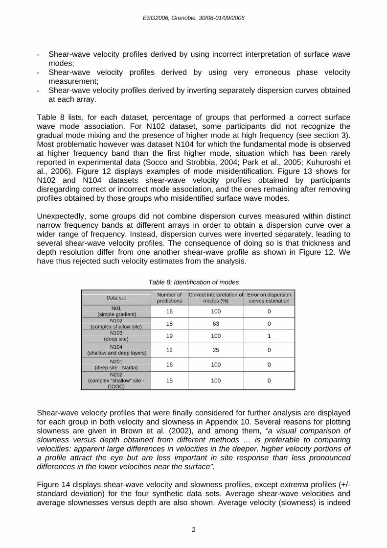
Table 8 lists, for each dataset, percentage of groups that performed a correct surface wave mode association. For N102 dataset, some participants did not recognize the gradual mode mixing and the presence of higher mode at high frequency (see section 3). Most problematic however was dataset N104 for which the fundamental mode is observed at higher frequency band than the first higher mode, situation which has been rarely reported in experimental data (Socco and Strobbia, 2004; Park et al., 2005; Kuhuroshi et al., 2006). Figure 12 displays examples of mode misidentification. Figure 13 shows for N102 and N104 datasets shear-wave velocity profiles obtained by participants disregarding correct or incorrect mode association, and the ones remaining after removing profiles obtained by those groups who misidentified surface wave modes. Unexpectedly, some groups did not combine dispersion curves measured within distinct narrow frequency bands at different arrays in order to obtain a dispersion curve over a wider range of frequency. Instead, dispersion curves were inverted separately, leading to several shear-wave velocity profiles. The consequence of doing so is that thickness and depth resolution differ from one another shear-wave profile as shown in Figure 12. We have thus rejected such velocity estimates from the analysis.

Table 8: Identification of modes

Data set Number of predictions

Correct interpretation of modes (%)

Error on dispersion curves estimation

N01 (simple gradient) 16 100 0

N102 (complex shallow site) 18 63 0

N103 (deep site) 19 100 1

N104 (shallow and deep layers) 12 25 0

N201 (deep site - Narita) 16 100 0

N202 (complex "shallow" site -

CCOC) 15 100 0

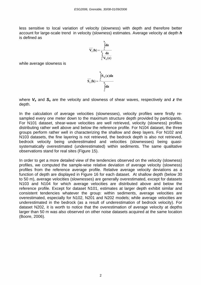
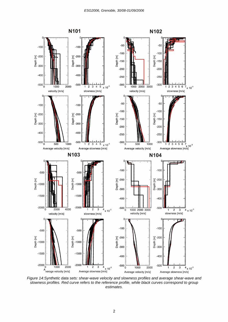
Shear-wave velocity profiles that were finally considered for further analysis are displayed for each group in both velocity and slowness in Appendix 10. Several reasons for plotting slowness are given in Brown et al. (2002), and among them, “a visual comparison of slowness versus depth obtained from different methods … is preferable to comparing velocities: apparent large differences in velocities in the deeper, higher velocity portions of a profile attract the eye but are less important in site response than less pronounced differences in the lower velocities near the surface”. Figure 14 displays shear-wave velocity and slowness profiles, except extrema profiles (+/- standard deviation) for the four synthetic data sets. Average shear-wave velocities and average slownesses versus depth are also shown. Average velocity (slowness) is indeed

ESG2006, Grenoble, 30/08-01/09/2006

2

less sensitive to local variation of velocity (slowness) with depth and therefore better account for large-scale trend in velocity (slowness) estimates. Average velocity at depth h is defined as

∫

∫= h

S

h

s

zVdz

dzhV

0

0

)(

)(

while average slowness is

∫

∫= h

h

S

s

dz

dzzShS

0

0

)()(

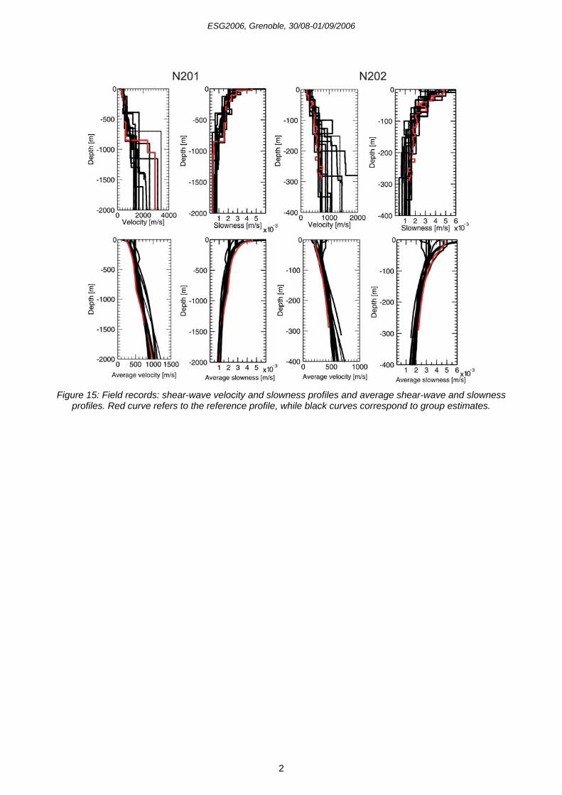
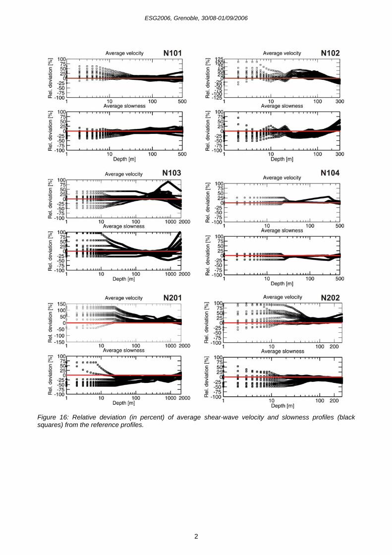
where Vs and Ss are the velocity and slowness of shear waves, respectively and z the depth. In the calculation of average velocities (slownesses), velocity profiles were firstly re-sampled every one meter down to the maximum structure depth provided by participants. For N101 dataset, shear-wave velocities are well retrieved, velocity (slowness) profiles distributing rather well above and below the reference profile. For N104 dataset, the three groups perform rather well in characterizing the shallow and deep layers. For N102 and N103 datasets, the fine layering is not retrieved, the bedrock depth is also not retrieved, bedrock velocity being underestimated and velocities (slownesses) being quasi-systematically overestimated (underestimated) within sediments. The same qualitative observations stand for real sites (Figure 15). In order to get a more detailed view of the tendencies observed on the velocity (slowness) profiles, we computed the sample-wise relative deviation of average velocity (slowness) profiles from the reference average profile. Relative average velocity deviations as a function of depth are displayed in Figure 16 for each dataset. At shallow depth (below 30 to 50 m), average velocities (slownesses) are generally overestimated, except for datasets N103 and N104 for which average velocities are distributed above and below the reference profile. Except for dataset N101, estimates at larger depth exhibit similar and consistent tendencies whatever the group: within sediments, average velocities are overestimated, especially for N102, N201 and N202 models; while average velocities are underestimated in the bedrock (as a result of underestimation of bedrock velocity). For dataset N202, it is worth to notice that the overestimation of average velocity at depths larger than 50 m was also observed on other noise datasets acquired at the same location (Boore, 2006).

ESG2006, Grenoble, 30/08-01/09/2006

2

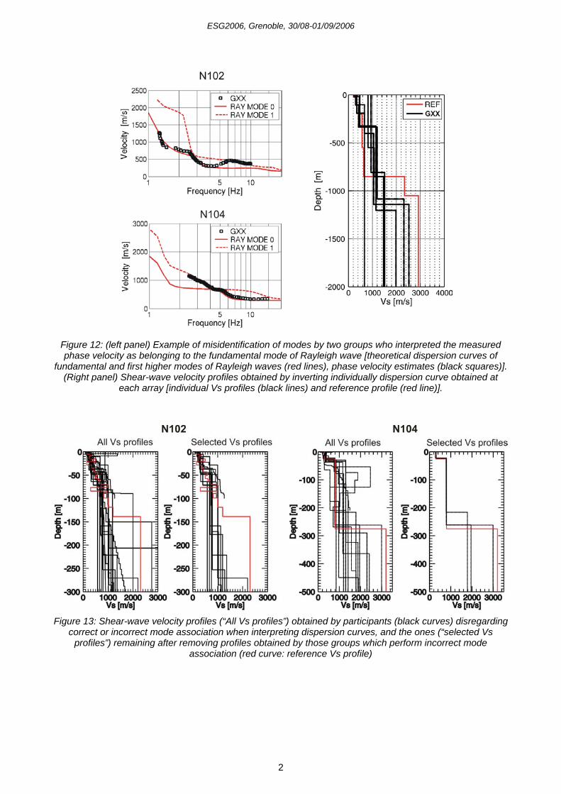
Figure 12: (left panel) Example of misidentification of modes by two groups who interpreted the measured phase velocity as belonging to the fundamental mode of Rayleigh wave [theoretical dispersion curves of

fundamental and first higher modes of Rayleigh waves (red lines), phase velocity estimates (black squares)]. (Right panel) Shear-wave velocity profiles obtained by inverting individually dispersion curve obtained at

each array [individual Vs profiles (black lines) and reference profile (red line)].

Figure 13: Shear-wave velocity profiles (“All Vs profiles”) obtained by participants (black curves) disregarding

correct or incorrect mode association when interpreting dispersion curves, and the ones (“selected Vs profiles”) remaining after removing profiles obtained by those groups which perform incorrect mode

association (red curve: reference Vs profile)

ESG2006, Grenoble, 30/08-01/09/2006

2

Figure 14:Synthetic data sets: shear-wave velocity and slowness profiles and average shear-wave and

slowness profiles. Red curve refers to the reference profile, while black curves correspond to group estimates.

ESG2006, Grenoble, 30/08-01/09/2006

2

Figure 15: Field records: shear-wave velocity and slowness profiles and average shear-wave and slowness

profiles. Red curve refers to the reference profile, while black curves correspond to group estimates.

ESG2006, Grenoble, 30/08-01/09/2006

2

Figure 16: Relative deviation (in percent) of average shear-wave velocity and slowness profiles (black squares) from the reference profiles.

ESG2006, Grenoble, 30/08-01/09/2006

2

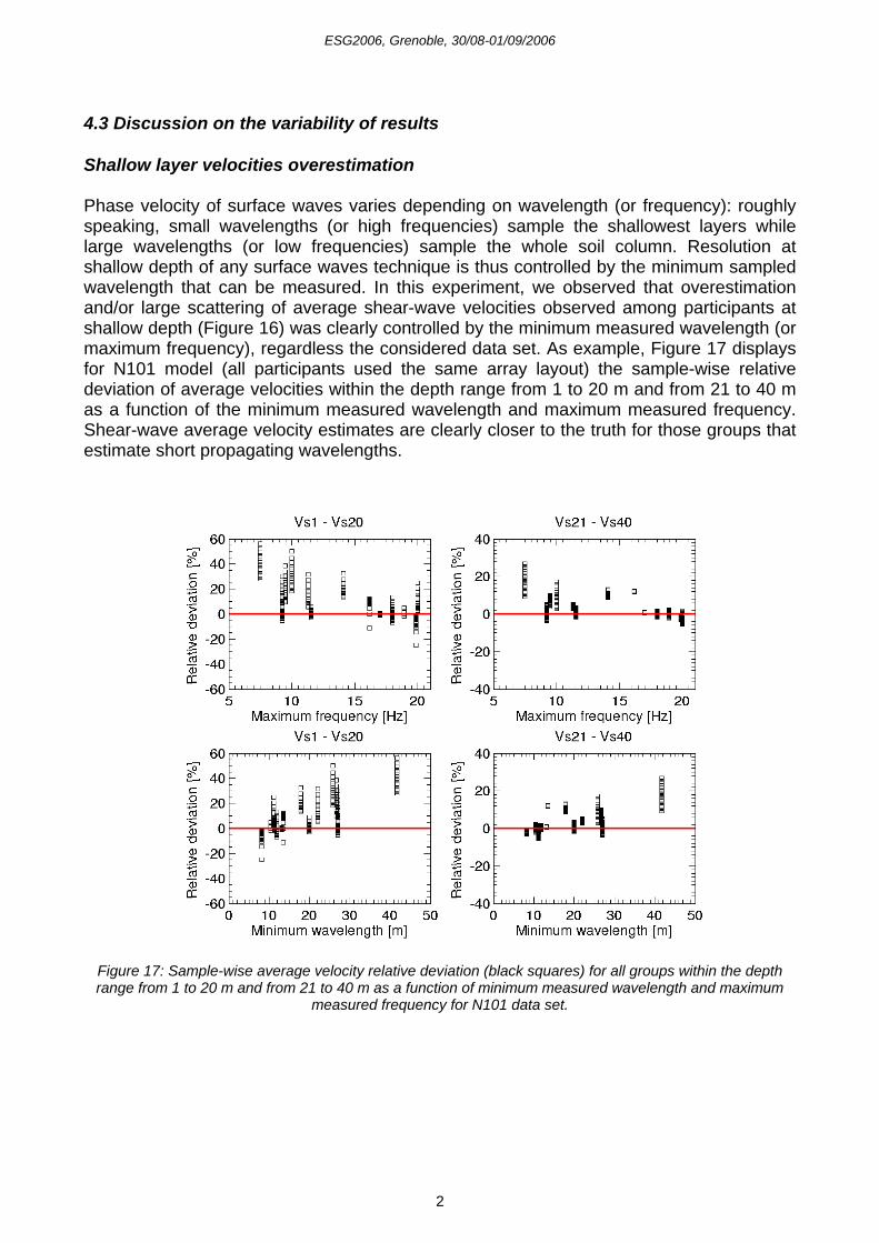
4.3 Discussion on the variability of results Shallow layer velocities overestimation Phase velocity of surface waves varies depending on wavelength (or frequency): roughly speaking, small wavelengths (or high frequencies) sample the shallowest layers while large wavelengths (or low frequencies) sample the whole soil column. Resolution at shallow depth of any surface waves technique is thus controlled by the minimum sampled wavelength that can be measured. In this experiment, we observed that overestimation and/or large scattering of average shear-wave velocities observed among participants at shallow depth (Figure 16) was clearly controlled by the minimum measured wavelength (or maximum frequency), regardless the considered data set. As example, Figure 17 displays for N101 model (all participants used the same array layout) the sample-wise relative deviation of average velocities within the depth range from 1 to 20 m and from 21 to 40 m as a function of the minimum measured wavelength and maximum measured frequency. Shear-wave average velocity estimates are clearly closer to the truth for those groups that estimate short propagating wavelengths.

Figure 17: Sample-wise average velocity relative deviation (black squares) for all groups within the depth range from 1 to 20 m and from 21 to 40 m as a function of minimum measured wavelength and maximum

measured frequency for N101 data set.

ESG2006, Grenoble, 30/08-01/09/2006

3

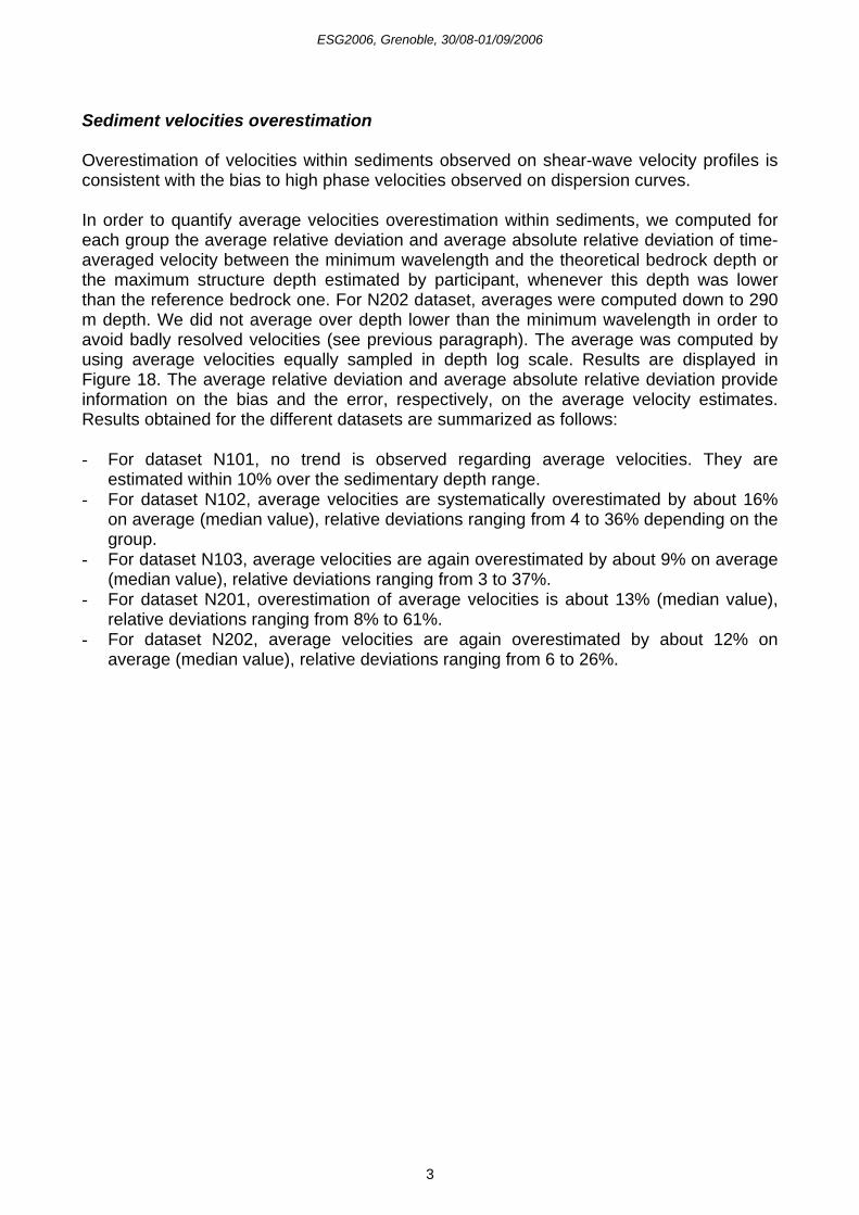
Sediment velocities overestimation Overestimation of velocities within sediments observed on shear-wave velocity profiles is consistent with the bias to high phase velocities observed on dispersion curves. In order to quantify average velocities overestimation within sediments, we computed for each group the average relative deviation and average absolute relative deviation of time-averaged velocity between the minimum wavelength and the theoretical bedrock depth or the maximum structure depth estimated by participant, whenever this depth was lower than the reference bedrock one. For N202 dataset, averages were computed down to 290 m depth. We did not average over depth lower than the minimum wavelength in order to avoid badly resolved velocities (see previous paragraph). The average was computed by using average velocities equally sampled in depth log scale. Results are displayed in Figure 18. The average relative deviation and average absolute relative deviation provide information on the bias and the error, respectively, on the average velocity estimates. Results obtained for the different datasets are summarized as follows: - For dataset N101, no trend is observed regarding average velocities. They are

estimated within 10% over the sedimentary depth range. - For dataset N102, average velocities are systematically overestimated by about 16%

on average (median value), relative deviations ranging from 4 to 36% depending on the group.

- For dataset N103, average velocities are again overestimated by about 9% on average (median value), relative deviations ranging from 3 to 37%.

- For dataset N201, overestimation of average velocities is about 13% (median value), relative deviations ranging from 8% to 61%.

- For dataset N202, average velocities are again overestimated by about 12% on average (median value), relative deviations ranging from 6 to 26%.

ESG2006, Grenoble, 30/08-01/09/2006

3

Figure 18: Average relative deviations and average absolute relative deviations of average velocities computed within the minimum wavelength measured by each group and the theoretical bedrock depth of

each site or the maximum structure depth estimated by participant, whenever this maximum depth was lower than the theoretical bedrock. Red circles indicate average values and grey patches stand for average values

+/- standard deviation.

ESG2006, Grenoble, 30/08-01/09/2006

3

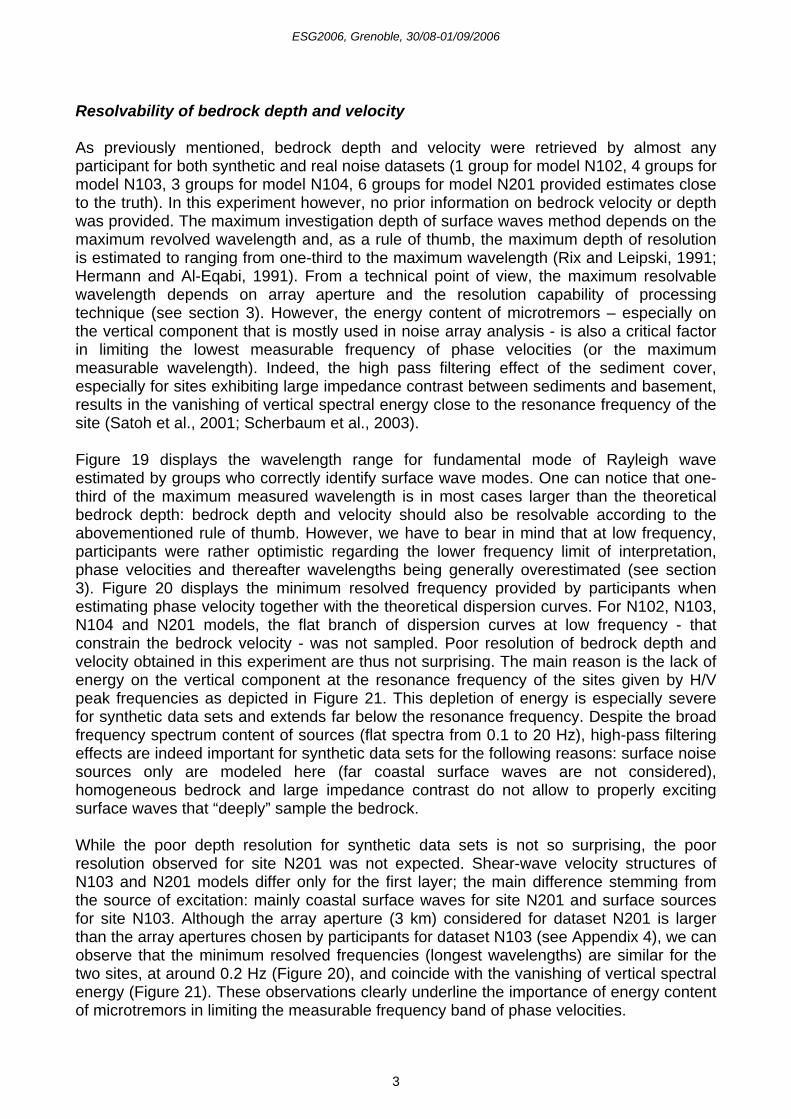
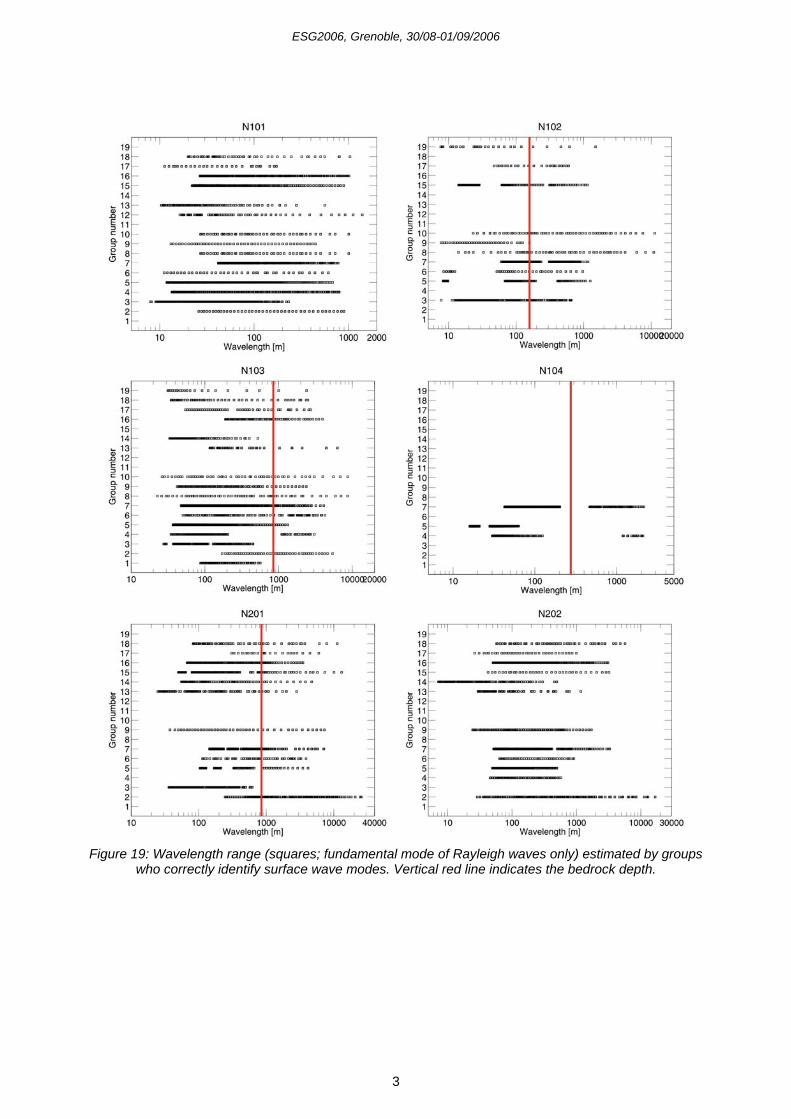
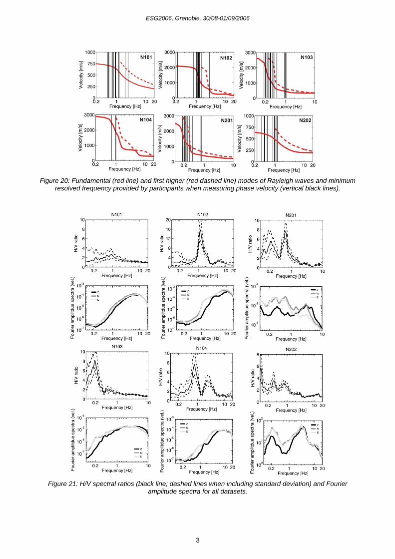
Resolvability of bedrock depth and velocity As previously mentioned, bedrock depth and velocity were retrieved by almost any participant for both synthetic and real noise datasets (1 group for model N102, 4 groups for model N103, 3 groups for model N104, 6 groups for model N201 provided estimates close to the truth). In this experiment however, no prior information on bedrock velocity or depth was provided. The maximum investigation depth of surface waves method depends on the maximum revolved wavelength and, as a rule of thumb, the maximum depth of resolution is estimated to ranging from one-third to the maximum wavelength (Rix and Leipski, 1991; Hermann and Al-Eqabi, 1991). From a technical point of view, the maximum resolvable wavelength depends on array aperture and the resolution capability of processing technique (see section 3). However, the energy content of microtremors – especially on the vertical component that is mostly used in noise array analysis - is also a critical factor in limiting the lowest measurable frequency of phase velocities (or the maximum measurable wavelength). Indeed, the high pass filtering effect of the sediment cover, especially for sites exhibiting large impedance contrast between sediments and basement, results in the vanishing of vertical spectral energy close to the resonance frequency of the site (Satoh et al., 2001; Scherbaum et al., 2003). Figure 19 displays the wavelength range for fundamental mode of Rayleigh wave estimated by groups who correctly identify surface wave modes. One can notice that one-third of the maximum measured wavelength is in most cases larger than the theoretical bedrock depth: bedrock depth and velocity should also be resolvable according to the abovementioned rule of thumb. However, we have to bear in mind that at low frequency, participants were rather optimistic regarding the lower frequency limit of interpretation, phase velocities and thereafter wavelengths being generally overestimated (see section 3). Figure 20 displays the minimum resolved frequency provided by participants when estimating phase velocity together with the theoretical dispersion curves. For N102, N103, N104 and N201 models, the flat branch of dispersion curves at low frequency - that constrain the bedrock velocity - was not sampled. Poor resolution of bedrock depth and velocity obtained in this experiment are thus not surprising. The main reason is the lack of energy on the vertical component at the resonance frequency of the sites given by H/V peak frequencies as depicted in Figure 21. This depletion of energy is especially severe for synthetic data sets and extends far below the resonance frequency. Despite the broad frequency spectrum content of sources (flat spectra from 0.1 to 20 Hz), high-pass filtering effects are indeed important for synthetic data sets for the following reasons: surface noise sources only are modeled here (far coastal surface waves are not considered), homogeneous bedrock and large impedance contrast do not allow to properly exciting surface waves that “deeply” sample the bedrock. While the poor depth resolution for synthetic data sets is not so surprising, the poor resolution observed for site N201 was not expected. Shear-wave velocity structures of N103 and N201 models differ only for the first layer; the main difference stemming from the source of excitation: mainly coastal surface waves for site N201 and surface sources for site N103. Although the array aperture (3 km) considered for dataset N201 is larger than the array apertures chosen by participants for dataset N103 (see Appendix 4), we can observe that the minimum resolved frequencies (longest wavelengths) are similar for the two sites, at around 0.2 Hz (Figure 20), and coincide with the vanishing of vertical spectral energy (Figure 21). These observations clearly underline the importance of energy content of microtremors in limiting the measurable frequency band of phase velocities.

ESG2006, Grenoble, 30/08-01/09/2006

3

Figure 19: Wavelength range (squares; fundamental mode of Rayleigh waves only) estimated by groups

who correctly identify surface wave modes. Vertical red line indicates the bedrock depth.

ESG2006, Grenoble, 30/08-01/09/2006

3

Figure 20: Fundamental (red line) and first higher (red dashed line) modes of Rayleigh waves and minimum

resolved frequency provided by participants when measuring phase velocity (vertical black lines).

Figure 21: H/V spectral ratios (black line; dashed lines when including standard deviation) and Fourier

amplitude spectra for all datasets.

ESG2006, Grenoble, 30/08-01/09/2006

3

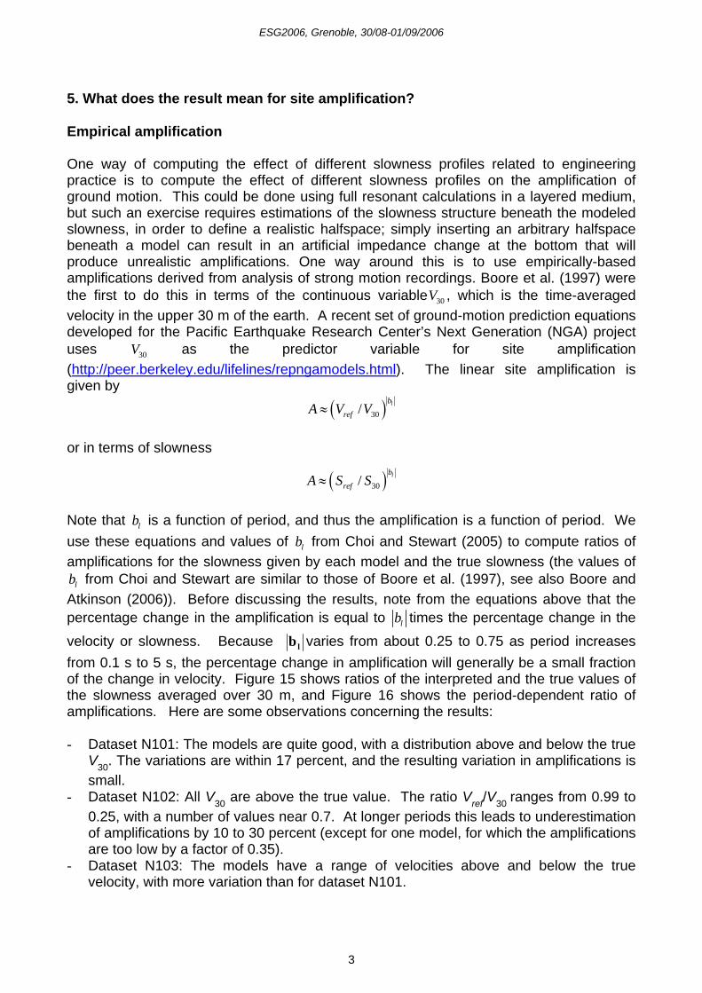
5. What does the result mean for site amplification? Empirical amplification One way of computing the effect of different slowness profiles related to engineering practice is to compute the effect of different slowness profiles on the amplification of ground motion. This could be done using full resonant calculations in a layered medium, but such an exercise requires estimations of the slowness structure beneath the modeled slowness, in order to define a realistic halfspace; simply inserting an arbitrary halfspace beneath a model can result in an artificial impedance change at the bottom that will produce unrealistic amplifications. One way around this is to use empirically-based amplifications derived from analysis of strong motion recordings. Boore et al. (1997) were the first to do this in terms of the continuous variable 30V , which is the time-averaged velocity in the upper 30 m of the earth. A recent set of ground-motion prediction equations developed for the Pacific Earthquake Research Center’s Next Generation (NGA) project uses 30V as the predictor variable for site amplification (http://peer.berkeley.edu/lifelines/repngamodels.html). The linear site amplification is given by

( )30/ lb

refA V V≈

or in terms of slowness

( )30/ lb

refA S S≈

Note that lb is a function of period, and thus the amplification is a function of period. We use these equations and values of lb from Choi and Stewart (2005) to compute ratios of amplifications for the slowness given by each model and the true slowness (the values of

lb from Choi and Stewart are similar to those of Boore et al. (1997), see also Boore and Atkinson (2006)). Before discussing the results, note from the equations above that the percentage change in the amplification is equal to lb times the percentage change in the

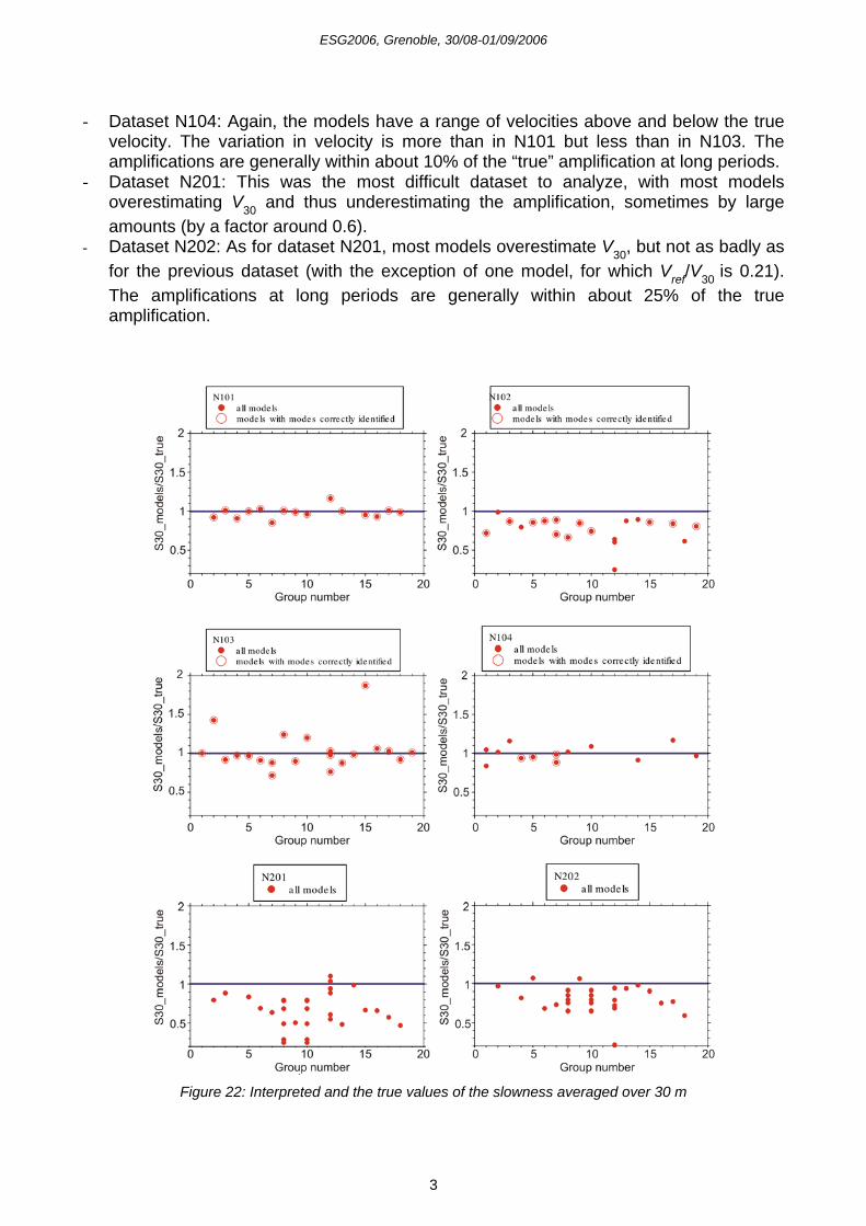
velocity or slowness. Because lb varies from about 0.25 to 0.75 as period increases from 0.1 s to 5 s, the percentage change in amplification will generally be a small fraction of the change in velocity. Figure 15 shows ratios of the interpreted and the true values of the slowness averaged over 30 m, and Figure 16 shows the period-dependent ratio of amplifications. Here are some observations concerning the results: - Dataset N101: The models are quite good, with a distribution above and below the true

V30. The variations are within 17 percent, and the resulting variation in amplifications is small.

- Dataset N102: All V30 are above the true value. The ratio Vref/V30 ranges from 0.99 to 0.25, with a number of values near 0.7. At longer periods this leads to underestimation of amplifications by 10 to 30 percent (except for one model, for which the amplifications are too low by a factor of 0.35).

- Dataset N103: The models have a range of velocities above and below the true velocity, with more variation than for dataset N101.

ESG2006, Grenoble, 30/08-01/09/2006

3

- Dataset N104: Again, the models have a range of velocities above and below the true velocity. The variation in velocity is more than in N101 but less than in N103. The amplifications are generally within about 10% of the “true” amplification at long periods.

- Dataset N201: This was the most difficult dataset to analyze, with most models overestimating V30 and thus underestimating the amplification, sometimes by large amounts (by a factor around 0.6).

- Dataset N202: As for dataset N201, most models overestimate V30, but not as badly as for the previous dataset (with the exception of one model, for which Vref/V30 is 0.21). The amplifications at long periods are generally within about 25% of the true amplification.

Figure 22: Interpreted and the true values of the slowness averaged over 30 m

ESG2006, Grenoble, 30/08-01/09/2006

3

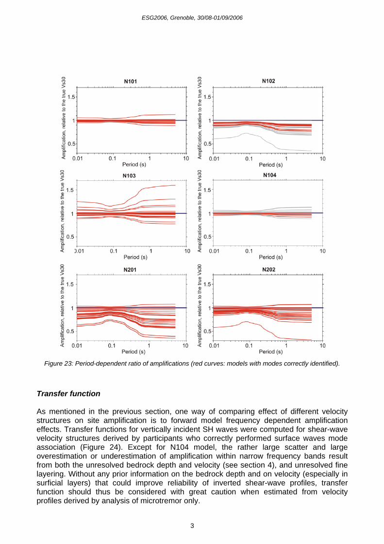
Figure 23: Period-dependent ratio of amplifications (red curves: models with modes correctly identified).

Transfer function As mentioned in the previous section, one way of comparing effect of different velocity structures on site amplification is to forward model frequency dependent amplification effects. Transfer functions for vertically incident SH waves were computed for shear-wave velocity structures derived by participants who correctly performed surface waves mode association (Figure 24). Except for N104 model, the rather large scatter and large overestimation or underestimation of amplification within narrow frequency bands result from both the unresolved bedrock depth and velocity (see section 4), and unresolved fine layering. Without any prior information on the bedrock depth and on velocity (especially in surficial layers) that could improve reliability of inverted shear-wave profiles, transfer function should thus be considered with great caution when estimated from velocity profiles derived by analysis of microtremor only.

ESG2006, Grenoble, 30/08-01/09/2006

3

Figure 24: (Top)Transfer functions (vertically incident SH waves) computed for velocity structures derived by participants (grey lines) and reference profile (red line). Vp values are taken as two times Vs values, density

are fixed to 2 kg/m3 and quality factors are similar to the ones used for noise computation (see Appendix 1).Transfer function are smoothed following the procedure of Konno and Ohmachi (1998) (b=20). (Bottom) Relative deviation (in percent) of amplification from the true amplification. N202 site is not considered here

since the reference profile is not known down to basement depth.

ESG2006, Grenoble, 30/08-01/09/2006

3

6. Discussion and Conclusions The aim of this blind test experiment was to assess the reliability of ambient vibration array analysis methods for estimating the shear-wave velocity structure, in the absence of any geological and geophysical information on site. In order to achieve this objective we separated the evaluation of the individual parts of the processing chain. 6.1 Derivation of dispersion curves The initial step consists in the estimation of surface wave dispersion curves from the recorded data. Four synthetic data sets have been created for this task to enable a comparison of estimated phase velocities to ‘ground truth’ information. Further real data sets have been added to compensate for deficiencies of the pure synthetic data sets (modeling of anthropogenic surface sources only). As it has been described in detail in section 3, the agreement between phase velocity estimates and theoretical values is not always satisfactory. We observe a tendency for phase velocity estimates of fundamental mode Rayleigh waves to be biased to higher velocities. We explain this observation mostly by insufficient resolution capabilities of the applied analysis methods with respect to the energetic contribution of multiple modes in the wavefields. Both f-k based techniques and spatial autocorrelation methods seem to be affected in a similar way by the existence of higher mode contributions in the wavefield and allow at most the estimation of an effective phase velocity (see also Tokimatsu et al., 1992a). Overestimation of phase velocities due to insufficient resolution at low frequencies for multiple signals arriving from different directions is stronger for f-k methods than for spatial autocorrelation methods. Therefore, although the number of participating groups seems too small to conclude statistically on the results, there is some indication that spatial autocorrelation methods perform better in the lower frequency range than f-k based methods. Similarly, Love wave fundamental dispersion curve estimation has been provided by only a small number of groups. Nonetheless, those phase velocity estimates surprisingly seem to be not biased and in general better than the corresponding Rayleigh wave dispersion curves. Due to this observation, it is unlikely that the existence of close sources to the arrays (as it is true at least for the synthetic data sets) and their corresponding contribution of curved wavefronts in the wavefield lead to the observed bias in estimating phase velocities from ambient vibration wavefields. An obvious and critical result of this blind test experiment has been the apparent difficulty in associating the estimated phase velocity samples to the correct surface wave mode branches when interpreting the dispersion curve results. Very strong differences among the participants have been observed in this interpretational issue. A similar interpretational problem seems to exist for the selection of the valid frequency band for the analysis and interpretation of results. Here, we observed a rather optimistic view among participants what regards the capabilities of a specific array configuration. In most cases, the groups chose to interpret analysis results in a larger frequency band than what is recommended in literature. 6.2 Derivation of shear-wave velocity profiles The second step of the processing chain consists in deriving the shear-waves velocity profiles from the dispersion curves. Regarding the inversion scheme, both direct search methods that generate random models into a bounded parameter space and linearized

ESG2006, Grenoble, 30/08-01/09/2006

4

and iterative methods were employed. Although the data to be inverted differed from group to group (fundamental mode, fundamental and higher modes, Rayleigh and Love waves), we did not recognize any “best” procedure or approach for inverting dispersion curves. Most obvious was the difficulty in estimating in a rational and meaningful way confidence levels on the derived shear-wave profiles, which is a crucial issue for site response evaluation purposes. Since misinterpretation of dispersion curves in terms of surface wave modes lead to incorrect shear-wave profiles, we disregarded such profiles when comparing shear-wave velocity estimates. Analysis of shear-wave profiles clearly outline that fine layering, basement depth and velocity were almost never retrieved for both synthetic and real data. We explain the poor bedrock resolution by the high pass filtering effect of the sedimentary cover, which leads to a depletion of vertical spectral content close to the resonance frequency of the site and, thereafter, limits the analyzable lower frequency band for phase velocity measurement. Consistently with overestimation of Rayleigh waves phase velocities, shear-wave velocities are systematically biased to higher velocities. When considering all groups estimates together, overestimation of time-averaged velocity averaged over the sediment cover is about 10-15%. 6.3 Consequences on site amplification The final aim of this experiment was to study effects of different shear-wave structures on site amplification. Empirical amplifications based on the time-averaged velocity over the uppermost 30 meters, V30, predict site amplification lower than the one expected by about 10 to 30% for synthetics having complex layering and real sites. This underestimation of site amplification reflects overestimation of V30. The forward modelling of frequency dependent amplification (SH transfer function) did not lead us to any conclusive remarks as regards effects of various velocity structures on site response. Basement depth and velocity, and fine layering not being resolved, transfer functions are indeed scattered. Without any better constrain on bedrock depth and velocity, SH transfer function is thus not a quantity that is recommended to directly estimate from velocity profiles derived by array analysis of microtremor only. At the present time, estimation of empirically-based amplification that only depends on time-averaged velocity seems a more robust prediction provided a proper design of array sizes for enabling shortest wavelengths sampling (see section 4) and a proper interpretation of surface wave modes. One of the main difficulties in this experiment was the lack of a priori knowledge regarding site conditions, which is often not the case for real world experiment. This exercise simply pinpointed that, today, ambient noise array technique should not be used for site response studies as a stand-alone tool without any other information on site condition or improvement in data processing and interpretation. Fortunately, for most of past studies “this method has been used for checking the reliability of results of other methods, by comparing the estimated structures or converting to other measurements” as mentioned by Okada (2003). Seismic ambient noise based techniques being however very cheap and thus attractive, doubtless is their spreading out as an alternative tool to classical geophysical ones for site imaging or site response purposes. This experiment highlighted some clear issues that should be addressed in the future for enabling site response estimates as accurate and reliable as possible: - An accurate interpretation of surface wave modes is definitely a prerequisite. This

interpretation is far from being straightforward and usually relies on “expert judgement”

ESG2006, Grenoble, 30/08-01/09/2006

4

as outlined in this experiment and also mentioned by Socco and Strobbia (2004) and Foti (2005): “Moreover the experimental dispersion curve is informative about trends to be expected by the final solution, so that its visual inspection is important for the qualitative validation of the results. Indeed engineering judgment plays a certain role in test interpretation. Since the site and the acquisition are never “ideal”, also the results of fully automated interpretation procedures must be carefully examined, with special attention to intermediate results during each step of the interpretation process. A deep knowledge of theoretical aspects and experience are hence essential.” Although interpretation of modes can be facilitated by the combined use of active and passive surface wave methods (Park et al, 2005; Rix, 2005), expert judgement still plays a large role in interpretation and should definitely be explicited in the future (through clear art-of-practice recommendations ?) ;

- Inversion procedures have to be improved for better constraining inverted shear-wave

profiles, issue which has been recently and is more and more addressed in literature. Besides technical improvement in inversion schemes or introduction of a priori information on site conditions, simultaneous inversion of both fundamental and higher modes or inversion of apparent phase velocity produced by modal superposition seems very promising to accurately estimate shear-wave velocity within sediments and to increase depth resolution (Tokimatsu, 1992a-b; Rix and Lai, 1998; Socco and Strobbia, 2004). Combined inversion of microtremor H/V and dispersion curves (Scherbaum et al., 2003; Arai and Tokimatsu, 2005; Parolai et al., 2005; Piccozi et al., 2005), or joint inversion of dispersion curves with other data types as gravity or earthquakes (e.g. Sakai and Morikawa, 2006, Kurose and Yamanaka, 2006) certainly brings additional and independent information on the target structure, especially in better constraining basement depth.

- Finally - and of special importance for engineering purposes - is the quantitative

evaluation of uncertainties and error propagation at each step of the processing chain in order to get robust shear-wave velocity estimates together with their confidence intervals in a meaningful way. Although some work has been very recently initiated towards quantitative assessment of uncertainties (Beaty et al, 2002; Comina et al., 2006; Dal Moro et al, 2007), this issue – that most often relies on an ad-hoc expert judgement – is still poorly addressed.

7. Acknowledgments We deeply thank all participants of this experiment. JNES (former NUPEC) kindly provided the geophysical/geotechnical data for Narita site, especially raw microtremor array data. Published data of geotechnical data by JNES (2005) were also used. Geotechnical data by NIED and Chiba Prefecture that have been published or opened on website were also used. We also thank Daniel Roten and Donat Fäh from ETH Zürich (Switzerland) and Alexandros Savaiidis from ITSAK (Thessaloniki, Greece) for providing us the real noise data for two real data sets. Computation of noise synthetics was performed at the Service Commun de Calcul Intensif de l'Observatoire de Grenoble (SCCI).

ESG2006, Grenoble, 30/08-01/09/2006

4

8. References Aki, K., 1957. Space and time spectra of stationary stochastic waves, with special reference to microtremors,

Bull. Earthq. Res. Inst. 35, 415-456. Almendros, J., J. M. Ibanez, G. Alguacil, E. Del Pezzo, 1999. Array analysis using circular-wave-front

geometry : an application to locate the nearby seismo-volcanic source, Geophys. J. Int., 136, 159-170. Arai, H. and K. Tokimatsu, 2005. S-Wave Profiling by Joint Inversion of Microtremor Dispersion Curve and

Horizontal-to-Vertical (H/V) Spectrum, Bull. Seism. Soc. Am., 95(5),1766-1778. Asten, M.W., and J.D. Henstridge, 1984. Array estimators and use of microseisms for reconnaissance of

sedimentary basins, Geophysics, 49, 1828-1837. Asten, M. W., Dhu, T., and Lam,N., 2004. Optimised array design for microtremor array studies applied to

site classification; observations, results and future use: Proceedings of the 13th World Conference of Earthquake Engineering, Vancouver, August 2004.

Asten, M. W. and D. M. Boore, 2005. Comparison of shear-velocity profiles of unconsolidated sediments near the Coyote borehole (CCOC) measured with fourteen invasive and non-invasive methods, Blind comparisons of shear-wave velocities at closely-spaced sites in San Jose, California, M. W. Asten and D. M. Boore (Editors), U. S. Geological Survey Open-File Report 2005-1169, part 1, 35 pp. [available on the World Wide Web at http://pubs.usgs.gov/of/2005/1169/].

Asten, M. W., 2005. An assessment of information on the shear-velocity profile at coyote Creek, San Jose, from SPAC processing of microtremor array data, extract from Asten and Boore (2005), USGS Open-File Report 2005-1169.

Beaty, K. S., D. R. Schmitt, m. Sacchi, 2002. Simulated annealing inversion of multimode Rayleigh wave dispersion curves for geological structure, Geophys. J. Int., 151, 622–631

Bettig, B., P. Y. Bard, F. Scherbaum, J. Riepl, F. Cotton, C. Cornou, and D. Hatzfeld, 2001, Analysis of dense array noise measurements using the modified spatial auto-correlation method MSPAC - Application to the Grenoble area: Bollettino di GeofisicaTeorica ed Applicata, 42, 281–304.

Boschetti, F., M. C. Dentith and R. D. List, 1996. Inversion of seismic refraction data using genetic algorithms, Geophysics 61, 1715-1727.

Boore, D.M. & Brown, L.T., 1998. Comparing shear-wave velocity profiles from inversion of surface-wave phase velocities with downhole measurements: systematic differences between the CXW method and downhole measurements at six USC strong-motion sites, Seism. Res. Lett, 69, 222–229.

Boore, M. W., 2006. Determining subsurface shear-wave velocities: a review, Proc. 3nd Int. Symp. on the Effects of Surface Geology on Seismic Motion, Grenoble, 29 August - 01 September, 2006, Bard, P.Y., Chaljub, E., Cornou, C., Cotton, F. and Guéguen, P. Editors, LCPC Editions, paper# 154

Boore, D. M., and G. M. Atkinson, 2006. Boore-Atkinson provisional NGA empirical ground-motion model for the average horizontal component of PGA, PGV and SA at spectral periods of 0.05, 0.1, 0.2, 0.3, 0.5, 1, 2, 3, 4, and 5 seconds, report to the PEER-Lifelines Next Generation Project [Revised 27 October 2006] [http://peer.berkeley.edu/lifelines/nga_docs/nov_13_06/Boore-Atkinson-NGA_11-13-06.html].

Boore, D. M., W. B. Joyner, and T. E. Fumal, 1997. Equations for estimating horizontal response spectra and peak acceleration from western North American earthquakes: A summary of recent work, Seism. Research Letters 68, 128-153.

Brown, L. T., D. M. Boore, and K. H. Stokoe, 2002. Comparison of shear-wave slowness profiles at ten strong-motion sites, Bull. Seism. Soc. Am. 92, 3116--3133

Burg, J.P., 1964. Three-dimensional filtering with an array of seismometers, Geophysics, 29, 693-713. Capon, J, 1969. High-Resolution frequency-wavenumber spectrum analysis. Proceedings of the IEEE, 57, 8,

1408-1418. Chiba Prefecture, 2005. The 2005 Report on the Under Ground Structure in Chiba Prefecture (CD-ROM, or

http://www.hp1039.jishin.go.jp/kozo/Chiba9/figures/f8-4.jpg) Cho, I., T. Tada, Y Shinozaki, 2004, A new method to determine phase velocities of Rayleigh waves from

microseisms, Geophysics, 69, 6, 1535-1551. Choi, Y. and J. P. Stewart, 2005. Nonlinear site amplification as function of 30 m shear wave velocity,

Earthquake Spectra 21, 1-30. Comina, C., D., Boiero, S., Foti, L. V. Socco, 2006. Noise blind test interpretation using f-k processing and

Monte Carlo inversion, Proc. 3nd Int. Symp. on the Effects of Surface Geology on Seismic Motion, Grenoble, 29 August - 01 September, 2006, Bard, P.Y., Chaljub, E., Cornou, C., Cotton, F. and Guéguen, P. Editors, LCPC Editions, paper #N04.

Cornou, C., P.-Y. Bard, M. Dietrich, 2003. Contribution of dense array analysis to the identification and quantification of basin-edge-induced waves, part I : methodology, Bulletin of the Seismological Society of America, 93, 6, 2604-2623.

ESG2006, Grenoble, 30/08-01/09/2006

4

Dal Moro, G., M. Pipan, P. Gabrielli, 2007. Rayleigh wave dispersion curve inversion via genetic algorithms and Marginal Posterior Probability Density estimation, Journal of Applied Geophysics, 61, 39–55.

Edwards, A. W. F., 1992. Likelihood, expanded edition, John Hopkins. Fäh, D., F. Kind and D. Giardini, 2003. Inversion of local S-wave velocity structures from average H/V ratios,

and their use for the estimation of site-effects, Journal of Seismology, 7, 449-467. Foti S., 2005. Surface Wave Testing for Geotechnical Characterization, in Surface Waves in Geomechanics:

Direct and Inverse Modelling for Soils and Rocks, CISM Series, Number 481, Lai C.G. and Wilmanski K. eds, Springer, Wien, 47-71

Gaffet, S., C. Larroque, A. Deschamps, and F. Tressols, 1998. A dense array experiment for the observation of waveform perturbations, Soil Dyn. Earthquake Eng. 17, 475–484.

Goldberg, D. E., 1989. Genetic Algorithms in Search, Optimization, and Machine Learning, Addison-Wesley, Reading, Massachusetts.

Hartzell, S., D. Carver, Tsuno S., Kudo K., Hermann, R., 2005. Shallow shear-wave velocity measurements in the Santa Clara Valley, comparison of spatial autocorrelation (SPAC) and frequency-wavenumber (FK) method, extract from Asten and Boore (2005) USGS Open-File Report 2005-1169.

Henstridge, J.D., 1979. A signal processing method for circular arrays, Geophysics, 44, 179–184. Herrmann, R. B., 1987. Surface wave inversion. Computer program in seismology, vol. 4, Saint Louis

University. Herrmann R.B., Al-Eqabi G.I., 1991. Surface wave inversion for shear velocity, in: J.M.Hoven et al. (eds),

Shear waves in marine sediments, Kluwer Academic Publisher, 545-556 Hisada, Y., 1994. An efficient method for computing Green's functions for a layered halfspace with sources

and receivers at close depths, Bull. Seism. Soc. Am., 84, 1456-1472. Hisada Y., 1995. An efficient method for computing Green's functions for a layered halfspace with sources

and receivers at close depths (Part 2). Bulletin of the Seismological Society of America, 85-4, 1080-1093.

Horike, M., 1985. Inversion of phase velocity of long-period microtremors to the S-wave-velocity structure down to the basement in urbanized areas, J. Phys. Earth, 33(2), 59-96.

JNES, 2005. The 2004 Fiscal Year Report of the Reliability Studies on Site Selection for Nuclear Power Plants, vol.1, Study on Methods for Evaluating Seismic Wave Propagation Characteristics (in Japanese)

Kanai, K., T. Tanaka, 1954. Measurement of microtremor, Bull. Earth. Res. Inst., 32, 199-209. Konno, K. and T. Ohmachi, 1998. Ground-motion characteristics estimated from spectral ratio between

horizontal and vertical components of microtremor. Bulletin of the Seismological Society of America, 88(1), 228-241.

Krim, H., and M. Viberg, 1996. Two decades of array signal processing research: the parametric approach, IEEE Signal Processing Mag. 13, 4, 67–94.

Kuhurashi, S., K. Masaki, Y. Sawada, L. Sugun, 2006. Verification of applicability of microtremor array survey, Proc. 3nd Int. Symp. on the Effects of Surface Geology on Seismic Motion, Grenoble, 29 August - 01 September, 2006, Bard, P.Y., Chaljub, E., Cornou, C., Cotton, F. and Guéguen, P. Editors, LCPC Editions, paper# 037.

Kurose, T., H. Yamanaka, 2006. Joint inversion of receiver function and surface-wave phase velocity for estimation of shear-wave velocity of sedimentary layers, Exploration Geophysics, 37, 93-101

Lacoss, R.T., Kelly, E.J., and M.N. Toksöz, 1969. Estimation of Seismic Noise Structure Using Arrays, Geophysics, 34(1), 21-38.

Ling, S., and H. Okada , 1993. An extended use of the spatial autocorrelation method for the estimation of structure using microtremors, in Proc. of the 89th SEGJ Conference, Nagoya, Japan, 12–14 October 1993, Society of Exploration Geophysicists of Japan, 44–48 (in Japanese).

Louie, J., 2001. Faster, Better: Shear-Wave Velocity to 100 Meters Depth from Refraction Microtremor Arrays, Bulletin of the Seismological Society of America, 91, 347-364.

Lomax, A, R. Snieder, 1994. Finding sets of acceptable solutions with a genetic algorithm with application to surface wave group dispersion in Europe, Geophys. Res. Lett., 27, 14, 2149-2152.

Miyakoshi K., 1996. A range of wavelengths possible to estimate phase velocities of surface waves in microtremors, Proc. of the 94th SEGJ Conf., Society of Exploration Geophysicists, Japan, 178-182 (in Japanese).

Moczo, P. and J. Kristek, 2002. “FD code to generate noise synthetics”, Sesame report D02.09, available on http://SESAME-FP5.obs.ujf-grenoble.fr

Morikawa, H., Sawada, S. and J. Akamatsu, 2004. A Method to Estimate Phase Velocities of Rayleigh Waves Using Microseims Simultaneously Observed at Two Sites, Bull. Seism. Soc. Am., 94(3), 961-976.

Mosegaard, K. and A. Tarantola, 1995. Monte Carlo Sampling of Solutions to Inverse Problems, Journal of Geophys. Res., 10, 12431-12447.

ESG2006, Grenoble, 30/08-01/09/2006

4

Nakamura,Y., 1989. A method for dynamic characteristics estimation of subsurface using microtremors on the ground surface, Quarterly reports of the RailwayTechnical Research InstituteTokyo, 30, 25–33.

Nogoshi M. and T. Igarashi, 1971. On the amplitude characteristics of microtremor (part 2) (in Japanese with english abstract). Journal of Seismological Society of Japan, 24, 26-40.

NUPEC, 2002. The 2001 Fiscal Year Report of the Reliability Studies on Site Selection for Nuclear Power Plants, vol.1, Study on Methods for Evaluating Seismic Wave Propagation Characteristics (in Japanese)

Okada, H., 2003. “The Microseismic Survey Method”, Society of Exploration Geophysicists of Japan. Translated by Koya Suto, Geophysical Monographs Vol 12. Tulsa: Society of Exploration Geophysicists, 2003.

Ohori, M., Nobata, A., and K. Wakamatsu, 2002. A Comparison of ESAC and FK Methods of Estimating Phase Velocity Using Arbitrarily Shaped Microtremor Arrays, Bull. Seism. Soc. Am., 92(6), 2323-2332.

Ohrnberger, M., Schissele, E., Cornou, C., Bonnefoy-Claudet, S., Wathelet, M., Savvaidis, A., Scherbaum F., and Jongmans, D., 2004. Frequency wavenumber and spatial autocorrelation methods for dispersion curve determination from ambient vibration recordings, Paper No. 0946, 13th World Conference on Earthquake Engineering, Vancouver, B.C., Canada.

Ohrnberger, M, 2005. Report on the FK/SPAC capabilities and limitations. SESAME Deliverable D19.06, 43 pp, http://sesame-fp5.obs.ujf-grenoble.fr/Delivrables/Del-D19-Wp06.pdf

Park, C.B., R.D. Miller, N. Ryden, J. Xia, J. Ivanov, 2005. Combined use of active and passive surface waves, JEEG, 10, 3, 323-334.

Parolai, S., Picozzi, M., Richwalski, S.M., and C. Milkereit, 2005. Joint Inversion of phase velocity dispersion and H/V ratio curves from seismic noise recordings using a genetic algorithm, considering higher modes, Geophys. Res. Letters, 32(1), L01303, doi: 10.1029/2004GL021115.

Picozzi, M., Parolai, S., and S. Richwalski, 2005. Joint Inversion H/V ratios and dispersion curves from seismic noise: Estimating the S-wave velocity of bedrock, Geophys. Res. Letter, 32(11), L11308, doi: 10.1029/2005GL022878.

Rix, G.J. & Leipski, E.A., 1991. Accuracy and Resolution of Surface Wave Inversion, pp. 17–32, Am. Soc. Civ. Eng.

Rix G.J., Lai C.G., 1998. Simultaneous inversion of surface wave velocity and attenuation, Geotechnical Site Characterization, Robertson & Mayne eds, vol. 1, Balkema, pp. 503-508

Rix, G.J., 2005. Near-surface site characterization using surface waves, Surface Waves in Geomechanics: Direct and Inverse Modelling for Soils and Rocks, C.G. Lai and K. Wilmanski, Eds., SpringerWien, New York, 1-46.

Roten, D., D. Fäh, C. Cornou, D. Giardini, 2006. 2D resonances in alpine valleys from ambient vibration wavefields, Geophysical Journal International, 165, doi: 10.1111/j.1365-246X.2006.02935.x.

Roten, D. and D. Fäh, 2006. A combined inversion of Rayleigh wave dispersion and 2D resonance frequencies, Geophysical Journal International, doi:10.1111/j.1365-246X.2006.03260.x

Rothman, D. H., 1985. Nonlinear inversion, statistical mechanics, and residual statics estimation, Geophysics, 50, 2784-2796.

Satoh, T., H. Kawase, T. Iwata, S. Higashi, T. Sato, K. Irikura, H.-C. huang, 2001. A-wave velocity structure of the Taichung basin, Taiwan, estimated from array and single-station records of microtremors, Bulletin of the Seismological Society of America, 91, 5, 1267–1282.

Sakai K., H. Morikawa, 2006. A method to estimate 2D subsurface structure using gravity and microtremor data and its application, Proc. 3nd Int. Symp. on the Effects of Surface Geology on Seismic Motion, Grenoble, 29 August - 01 September, 2006, Bard, P.Y., Chaljub, E., Cornou, C., Cotton, F. and Guéguen, P. Editors, LCPC Editions, paper #021.

Sambridge, M., 1999. Geophysical inversion with a neighbourhood algorithm: I. Searching a parameter space, Geophysical Journal International 138, 479-494.

Scherbaum F., Hinzen K.-G. and Ohrnberger M.; 2003: Determination of shallow shear wavevelocity profiles in the Cologne, Germany area using ambient vibrations, Geophys. J. Int., 152, 597-612.

Schissele, E., J. Guilbert, S. Gaffet, Y. Cansi, 2004. Accurate time-frequency-wavenumber analysis to study coda waves, Geophys. J. Int., 158, 577-591.

Schmidt, R., 1986. Multiple emitter location and signal parameter estimation, IEEE Trans. on Antennas and Propagation, 34(3), 276-280.

Sen, M. K. and P. L. Stoffa, 1991. Nonlinear one-dimensional seismic waveform inversion using simulated annealing, Geophysics, 56, 1624-1638.

Shapiro, N.M, M. Campillo, L. Stehly and M. Ritzwoller, 2005. High Resolution Surface Wave Tomography from Ambient Seismic Noise, Science, 307, 1615-1618

Shapiro N.M. and M. Campillo, 2004. Emergence of broadband Rayleigh waves from correlations of the ambient seismic noise, Geophys. Res. Letters, 31, L07614, doi:10.1029/2004GL019491

ESG2006, Grenoble, 30/08-01/09/2006

4

Socco, L. V. and C. Strobbia, 2004. Surface-wave method for near surface characterization: a tutorial. Near Surface Geophysics 2(4), 165–185.

Stephenson, W. J., J. N. Louie, S. Pullammanappallil, R. A. Williams, and J. K. Odum (2005). Blind shear-wave velocity comparison of ReMi and MASW results with boreholes to 200 m in Santa Clara Valley: Implications for earthquake ground-motion assessment, Bull. Seism. Soc. Am. 95, 2506–-2516.

Stoffa, P. L. and M. K. Sen,1991. Nonlinear multiparameter optimization using genetic algorithms: Inversion of plane-wave seismograms, Geophysics, 56, 1794-1810.

Tokimatsu, K., Tamura, Sh., and H. Kojima, 1992a. Effects of Multiple Modes on Rayleigh Wave Dispersion Characteristics, Journal of Geotechnical Engineering, 118(10), 1529-1543.

Tokimatsu, K., Shinzawa, K., and Sh. Kuwayama, 1992b. Use of Short-Period Microtremor ofr Vs Profiling, Journal of Geotechnical Engineering, 118(10), 1544-1558.

Tokimatsu, K., 1997. Geotechnical site characterization using surface waves, In: Proc. 1st Intl. Conf. Earthquake Geotechnical Engineering, Ishihara (ed), Balkema, 1333-1368.

Wathelet, M., D. Jongmans, and M. Ohrnberger, 2004. Surface wave inversion using a direct search algorithm and its application to ambient vibration measurements, Near Surface Geophysics, 2, 211-221

Wathelet, M. , D. Jongmans, and M. Ohrnberger (2005). Direct Inversion of Spatial Autocorrelation Curves with the Neighborhood Algorithm. Bulletin of the Seismological Society of America, 95, 1787-1800

Wentworth, C.M., and Tinsley, J.C., 2005. Detailed stratigraphy and velocity structure of Quaternary alluvial sediments, Santa Clara Valley, California: paper presented at the Annual Northern California Earthquake Hazards Workshop January 18-19,2005, USGS, Menlo Park.

Williams, R.A., Stephenson, W.J., Wentworth, C.M., Odum, J.K., Hanson, R.T., and R.C. Jachens, 2002. Definition of the Silver Creek fault and Evergreen Basin sediments from seismic reflection data, San Jose, California: EOS Transactions, Fall AGU meeting, v. 83, no. 47, p. F1313.

Woods, J.W., and P.L. Lintz, 1973. Plane waves at small arrays, Geophysics, 38, 1023-1041. Park, C.B., R.D. Miller, N. Ryden, J. Xia, J. Ivanov, 2005. Combined use of active and passive surface

waves, JEEG, 10, 3, 323-334. Yamanaka, H., Furuya, S., Nozawa, T., Sasaki T., and Takai, T., 1995. Array measurements of long-period

microtremors in the Kanto Plain -Estimation of S-wave velocity structure at Koto-: Journal of Structural and Construction Engineering, Architectural Institute of Japan, 478, 99–105.

Yamanaka, H. and H. Ishida, 1996. Application of genetic algorithms to an inversion of surface-wave dispersion data, Bull. Seism. Soc. Am. 86, 436-444

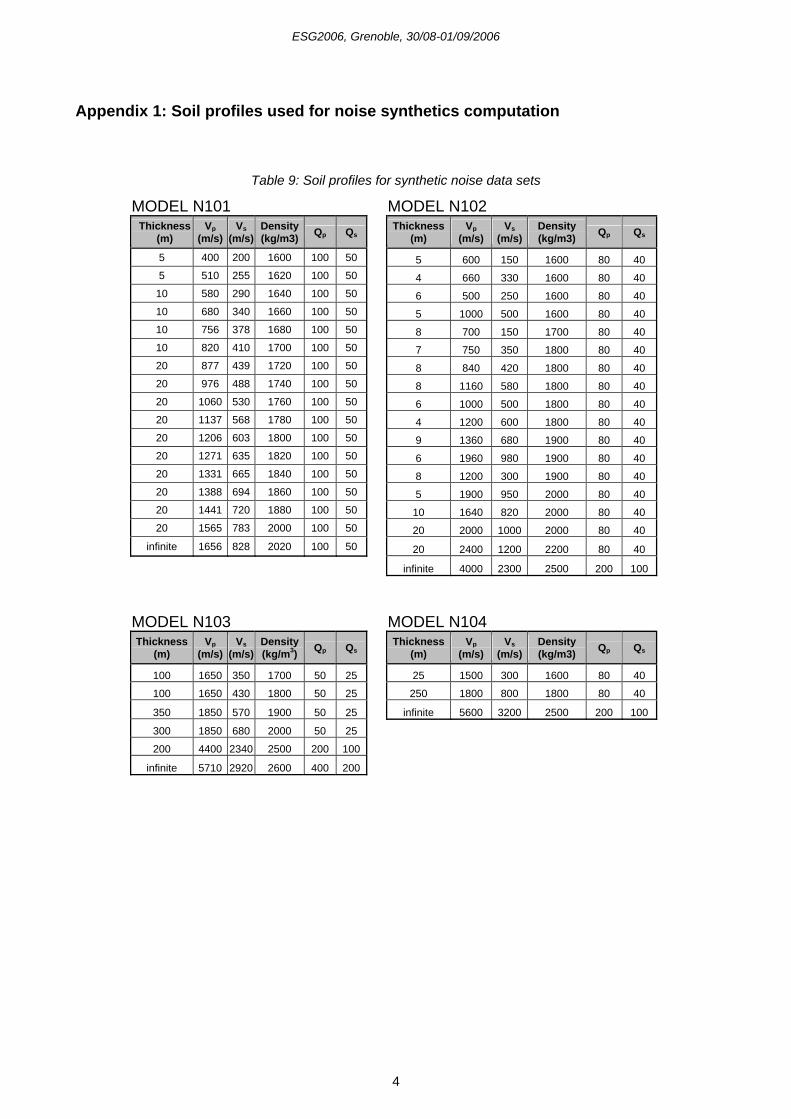
ESG2006, Grenoble, 30/08-01/09/2006

4

Appendix 1: Soil profiles used for noise synthetics computation

Table 9: Soil profiles for synthetic noise data sets

MODEL N101 MODEL N102 Thickness

(m) Vp

(m/s) Vs

(m/s) Density (kg/m3) Qp Qs

Thickness (m)

Vp (m/s)

Vs (m/s)

Density (kg/m3) Qp Qs

5 400 200 1600 100 50 5 600 150 1600 80 40 5 510 255 1620 100 50 4 660 330 1600 80 40

10 580 290 1640 100 50 6 500 250 1600 80 40 10 680 340 1660 100 50 5 1000 500 1600 80 40 10 756 378 1680 100 50 8 700 150 1700 80 40 10 820 410 1700 100 50 7 750 350 1800 80 40 20 877 439 1720 100 50 8 840 420 1800 80 40 20 976 488 1740 100 50 8 1160 580 1800 80 40 20 1060 530 1760 100 50 6 1000 500 1800 80 40 20 1137 568 1780 100 50 4 1200 600 1800 80 40 20 1206 603 1800 100 50 9 1360 680 1900 80 40 20 1271 635 1820 100 50 6 1960 980 1900 80 40 20 1331 665 1840 100 50 8 1200 300 1900 80 40 20 1388 694 1860 100 50 5 1900 950 2000 80 40 20 1441 720 1880 100 50 10 1640 820 2000 80 40 20 1565 783 2000 100 50 20 2000 1000 2000 80 40

infinite 1656 828 2020 100 50 20 2400 1200 2200 80 40

infinite 4000 2300 2500 200 100

MODEL N103 MODEL N104 Thickness

(m) Vp

(m/s) Vs

(m/s) Density (kg/m3) Qp Qs

Thickness (m)

Vp (m/s)

Vs (m/s)

Density (kg/m3) Qp Qs

100 1650 350 1700 50 25 25 1500 300 1600 80 40

100 1650 430 1800 50 25 250 1800 800 1800 80 40

350 1850 570 1900 50 25 infinite 5600 3200 2500 200 100

300 1850 680 2000 50 25 200 4400 2340 2500 200 100

infinite 5710 2920 2600 400 200

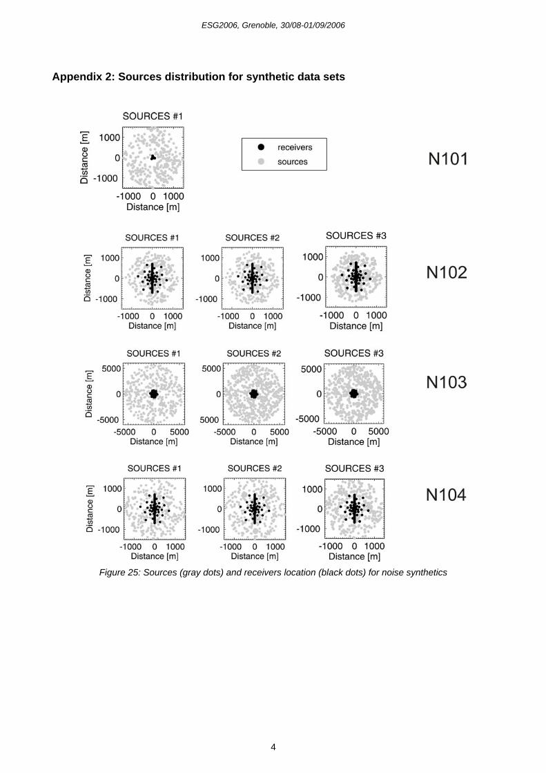
ESG2006, Grenoble, 30/08-01/09/2006

4

Appendix 2: Sources distribution for synthetic data sets

Figure 25: Sources (gray dots) and receivers location (black dots) for noise synthetics

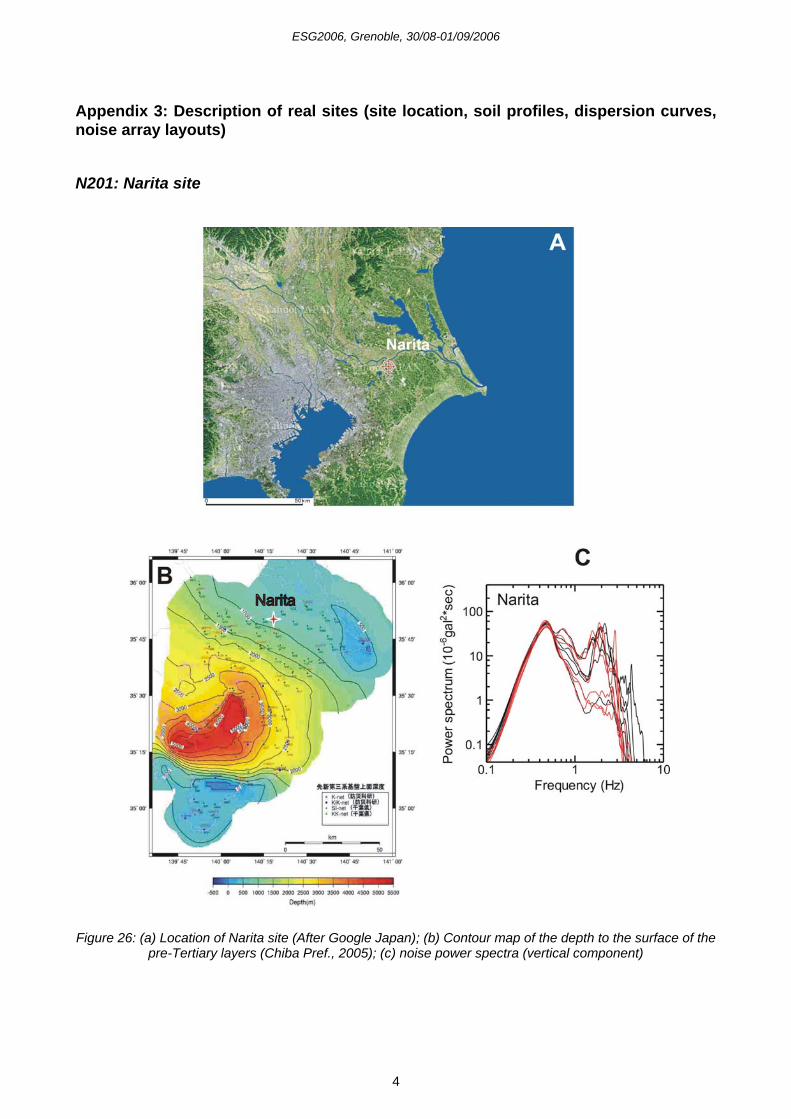
ESG2006, Grenoble, 30/08-01/09/2006

4

Appendix 3: Description of real sites (site location, soil profiles, dispersion curves, noise array layouts)

N201: Narita site

Figure 26: (a) Location of Narita site (After Google Japan); (b) Contour map of the depth to the surface of the

pre-Tertiary layers (Chiba Pref., 2005); (c) noise power spectra (vertical component)

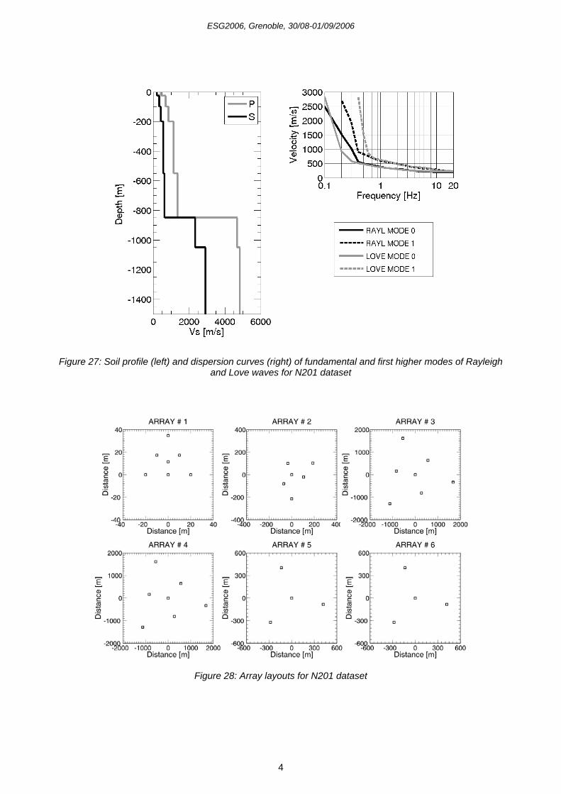
ESG2006, Grenoble, 30/08-01/09/2006

4

Figure 27: Soil profile (left) and dispersion curves (right) of fundamental and first higher modes of Rayleigh

and Love waves for N201 dataset

Figure 28: Array layouts for N201 dataset

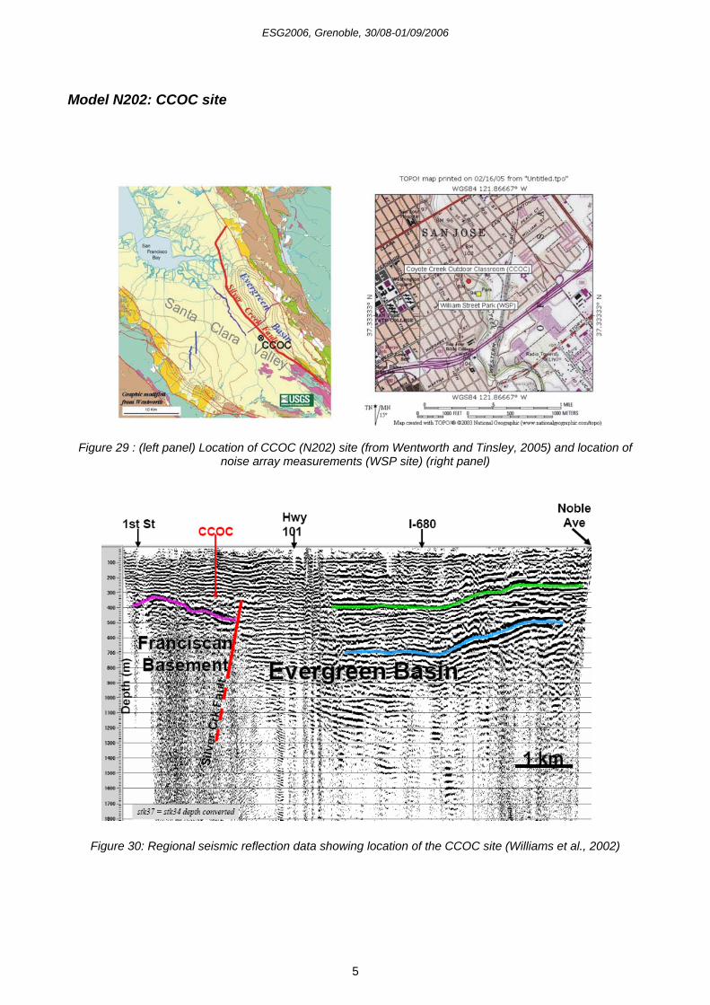
ESG2006, Grenoble, 30/08-01/09/2006

5

Model N202: CCOC site

Figure 29 : (left panel) Location of CCOC (N202) site (from Wentworth and Tinsley, 2005) and location of

noise array measurements (WSP site) (right panel)

Figure 30: Regional seismic reflection data showing location of the CCOC site (Williams et al., 2002)

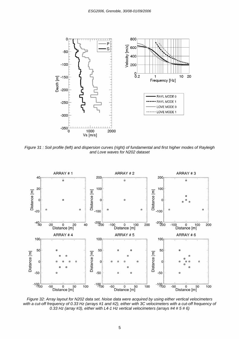
ESG2006, Grenoble, 30/08-01/09/2006

5

Figure 31 : Soil profile (left) and dispersion curves (right) of fundamental and first higher modes of Rayleigh

and Love waves for N202 dataset

Figure 32: Array layout for N202 data set. Noise data were acquired by using either vertical velocimeters

with a cut-off frequency of 0.33 Hz (arrays #1 and #2), either with 3C velocimeters with a cut-off frequency of 0.33 Hz (array #3), either with L4-1 Hz vertical velocimeters (arrays #4 # 5 # 6)

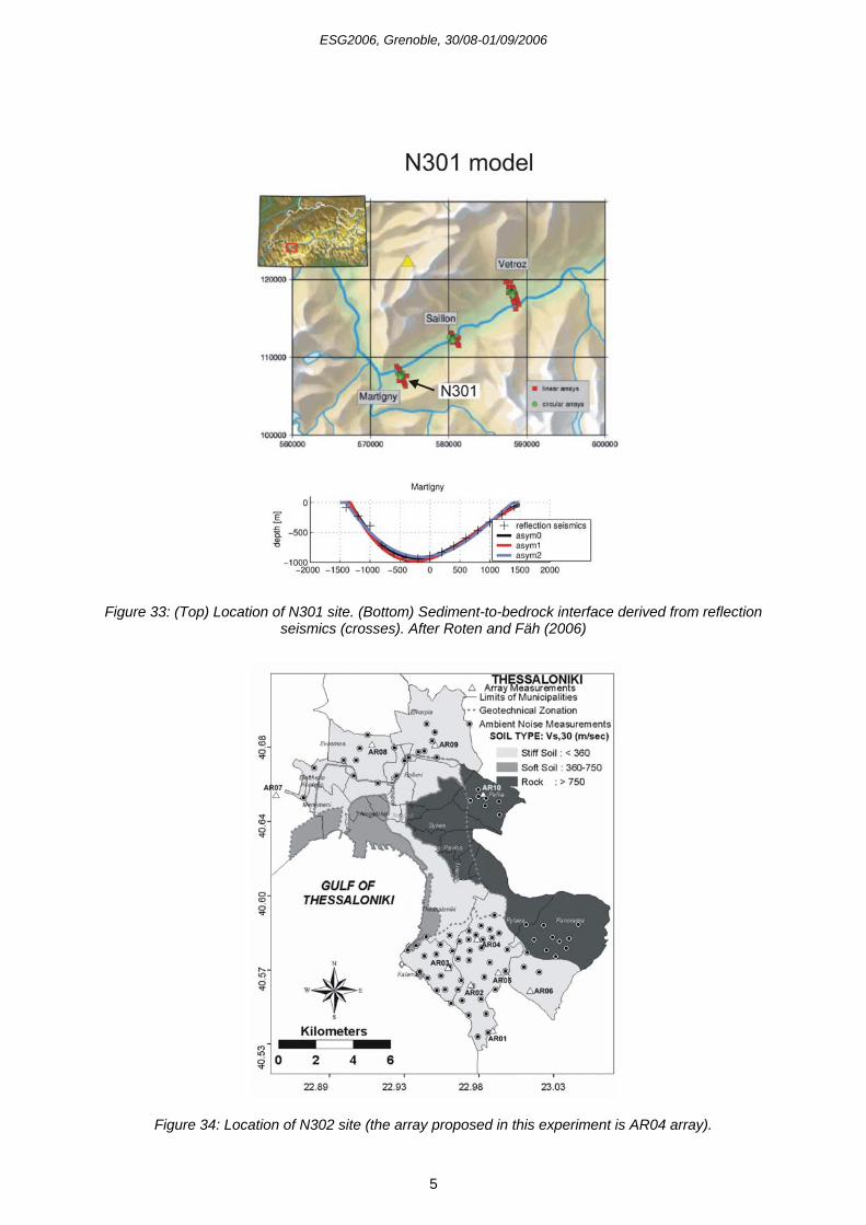
ESG2006, Grenoble, 30/08-01/09/2006

5

Figure 33: (Top) Location of N301 site. (Bottom) Sediment-to-bedrock interface derived from reflection

seismics (crosses). After Roten and Fäh (2006)

Figure 34: Location of N302 site (the array proposed in this experiment is AR04 array).

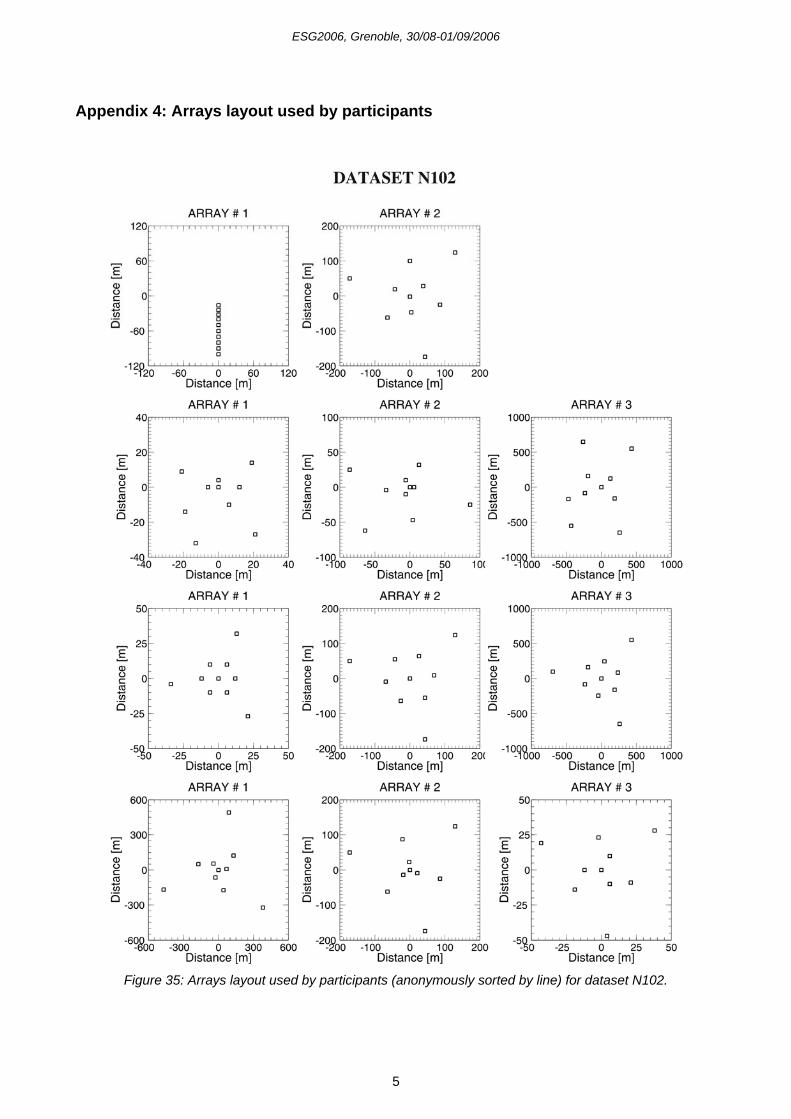
ESG2006, Grenoble, 30/08-01/09/2006

5

Appendix 4: Arrays layout used by participants

Figure 35: Arrays layout used by participants (anonymously sorted by line) for dataset N102.

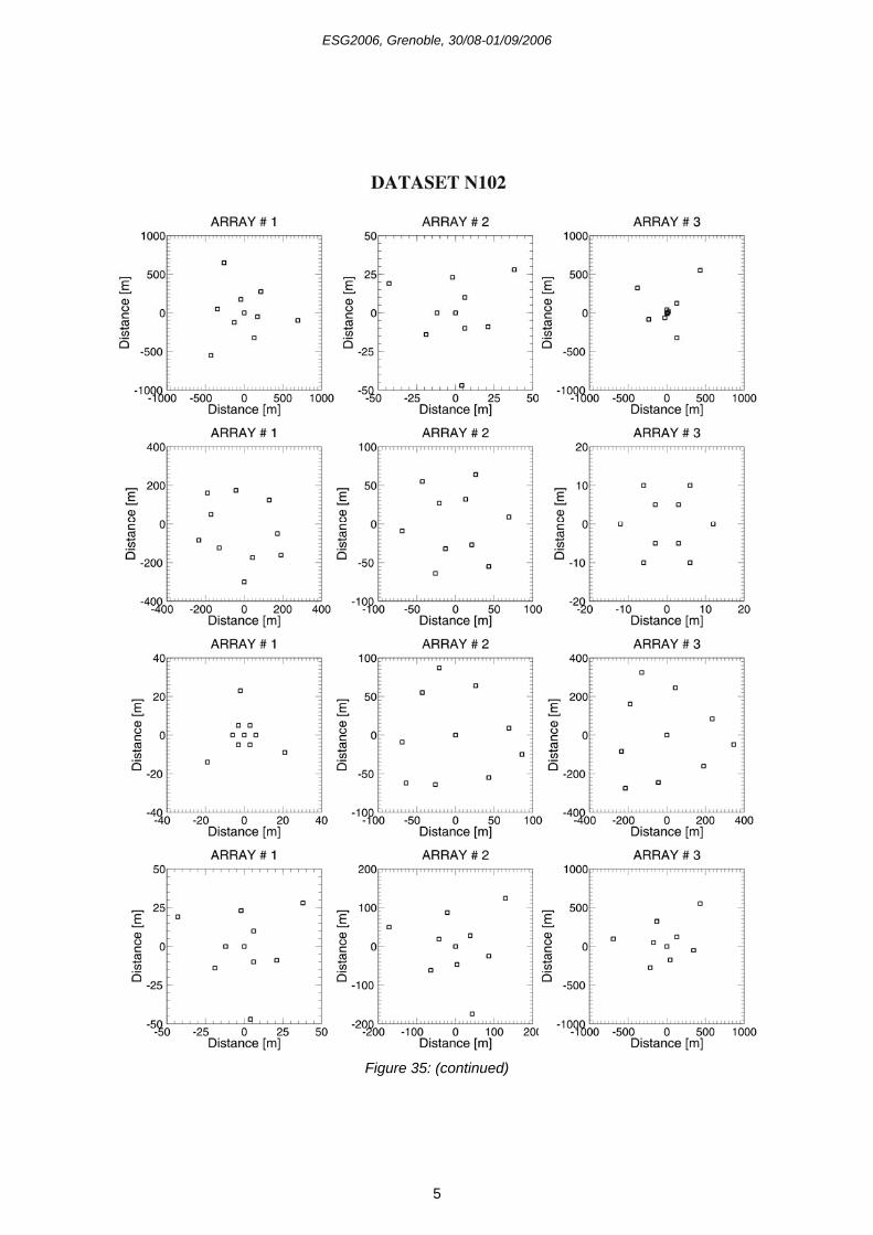
ESG2006, Grenoble, 30/08-01/09/2006

5

Figure 35: (continued)

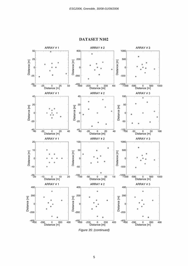
ESG2006, Grenoble, 30/08-01/09/2006

5

Figure 35: (continued)

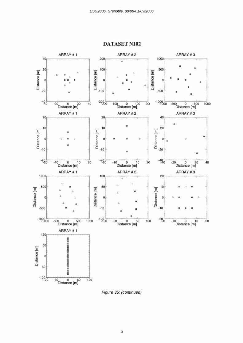
ESG2006, Grenoble, 30/08-01/09/2006

5

Figure 35: (continued)

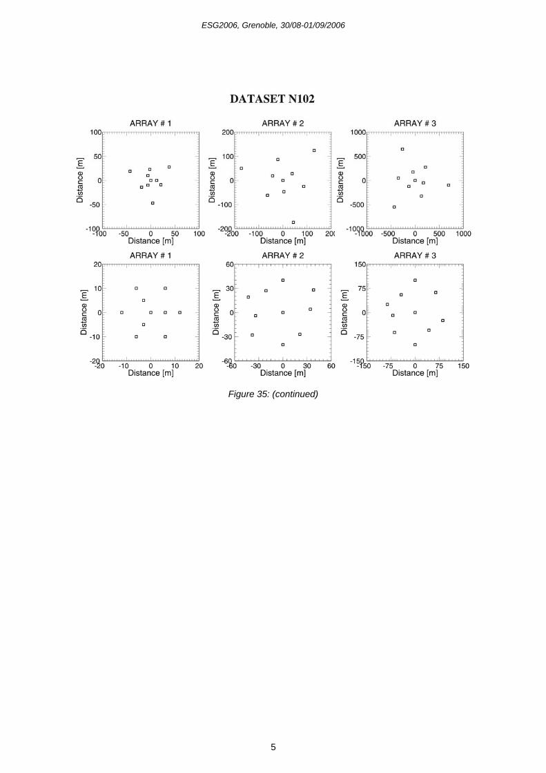
ESG2006, Grenoble, 30/08-01/09/2006

5

Figure 35: (continued)

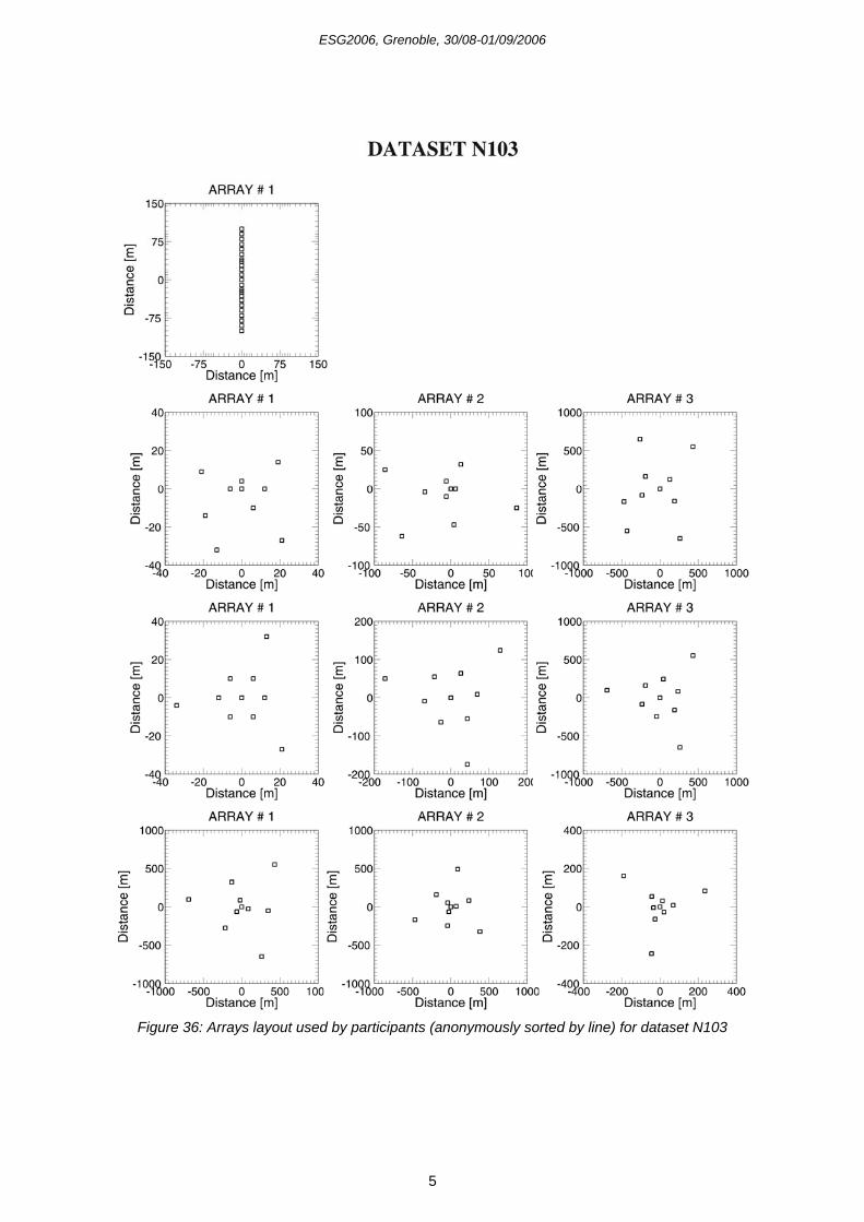
ESG2006, Grenoble, 30/08-01/09/2006

5

Figure 36: Arrays layout used by participants (anonymously sorted by line) for dataset N103

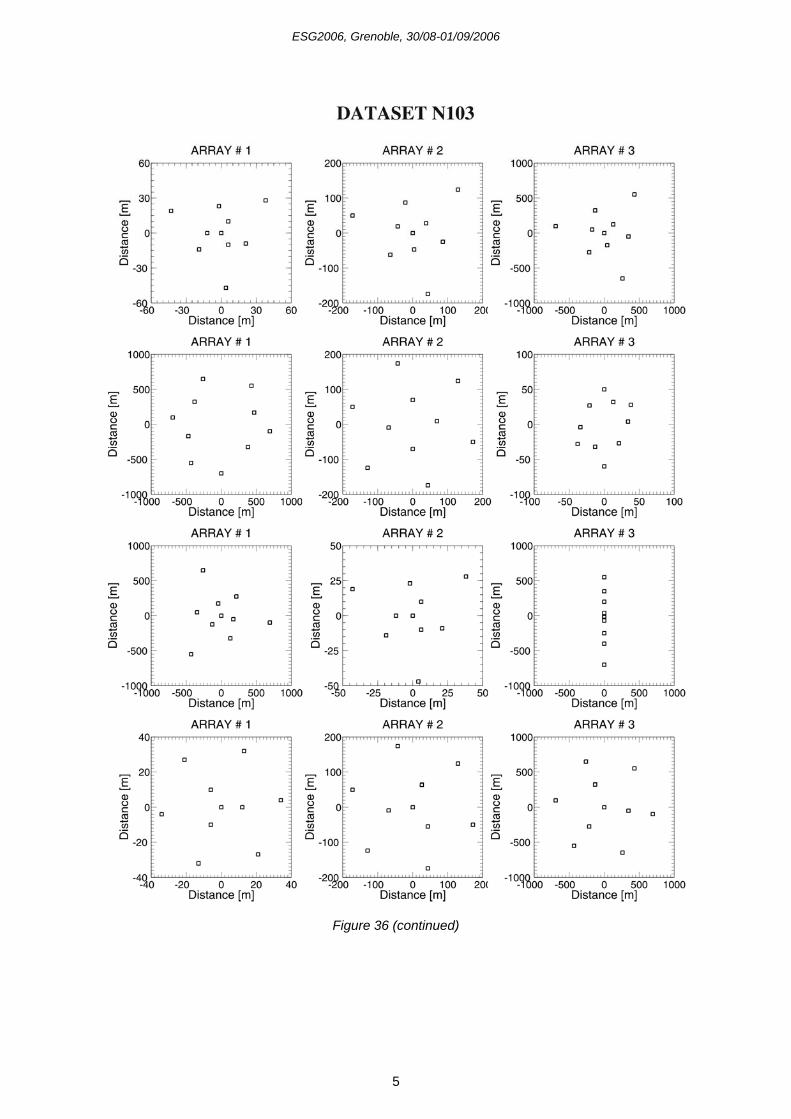
ESG2006, Grenoble, 30/08-01/09/2006

5

Figure 36 (continued)

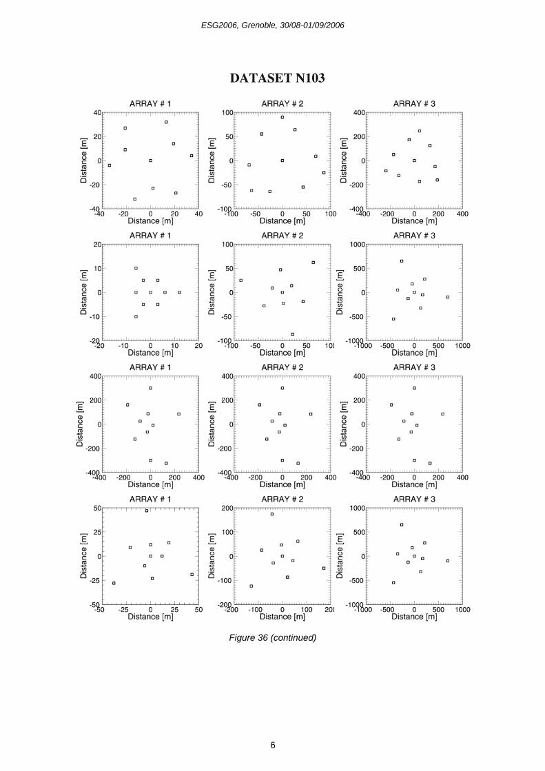
ESG2006, Grenoble, 30/08-01/09/2006

6

Figure 36 (continued)

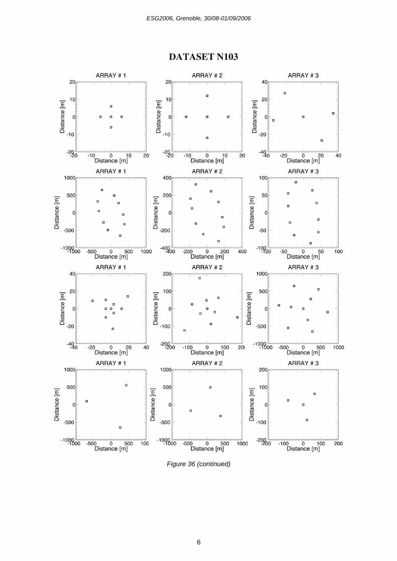
ESG2006, Grenoble, 30/08-01/09/2006

6

Figure 36 (continued)

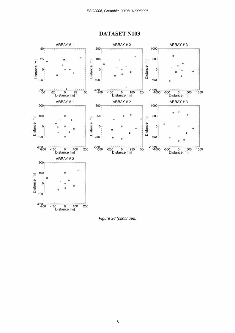
ESG2006, Grenoble, 30/08-01/09/2006

6

Figure 36 (continued)

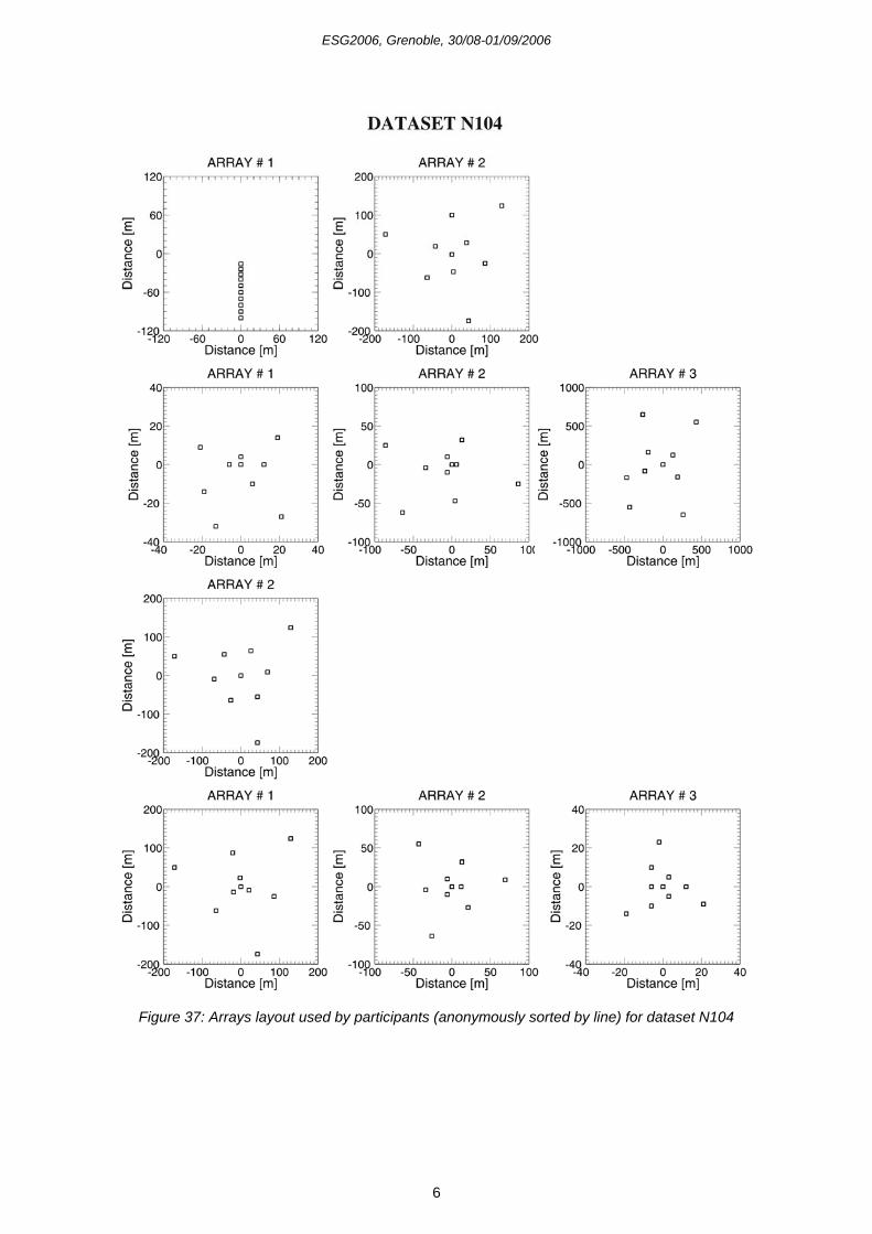
ESG2006, Grenoble, 30/08-01/09/2006

6

Figure 37: Arrays layout used by participants (anonymously sorted by line) for dataset N104

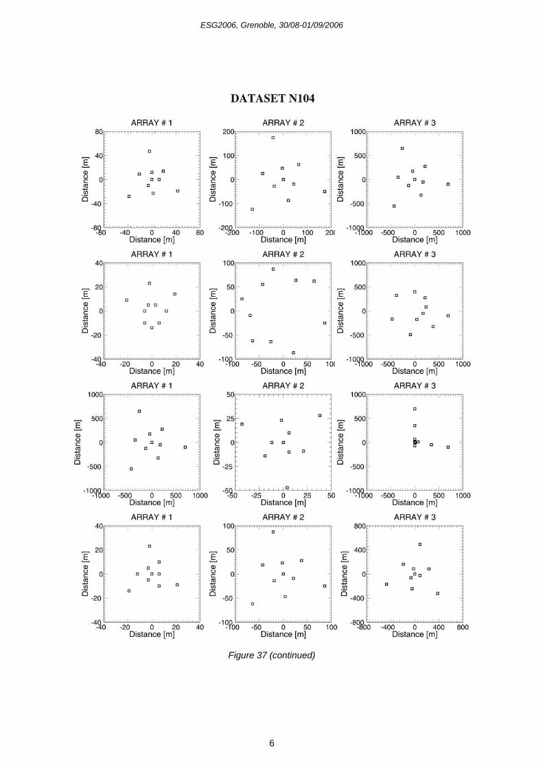
ESG2006, Grenoble, 30/08-01/09/2006

6

Figure 37 (continued)

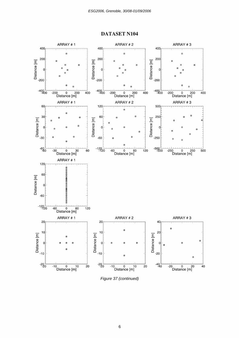
ESG2006, Grenoble, 30/08-01/09/2006

6

Figure 37 (continued)

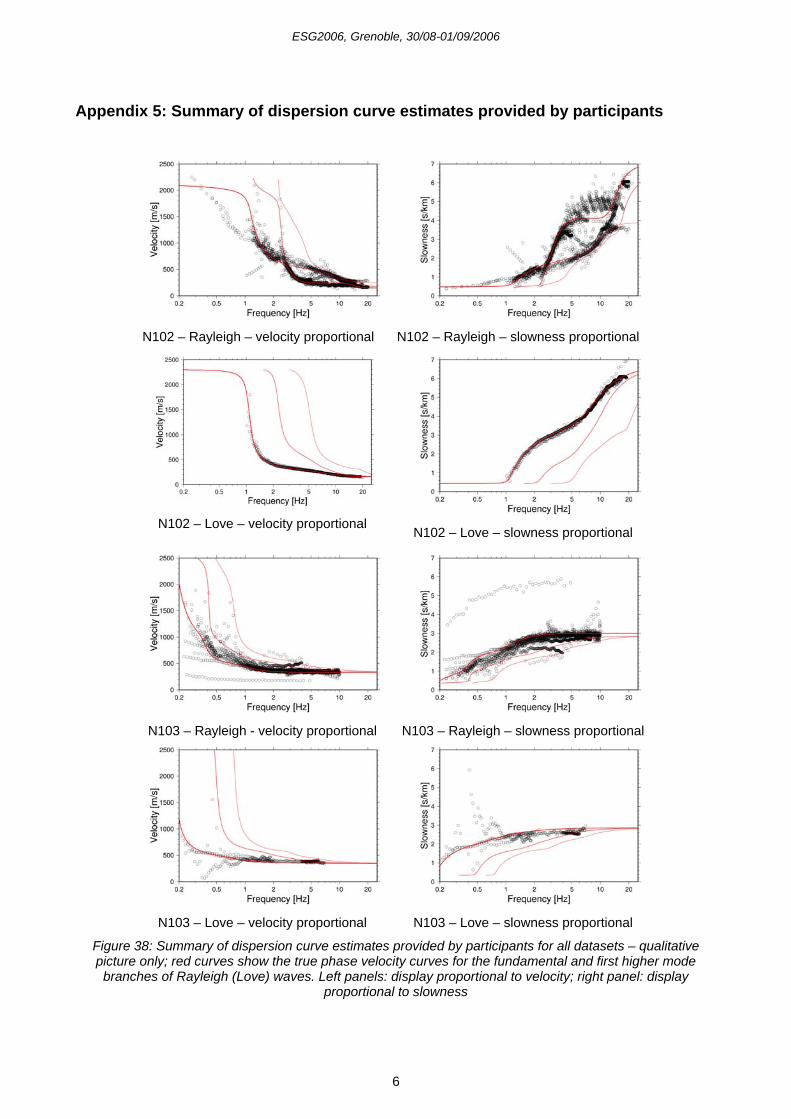
ESG2006, Grenoble, 30/08-01/09/2006

6

Appendix 5: Summary of dispersion curve estimates provided by participants

N102 – Rayleigh – velocity proportional

N102 – Rayleigh – slowness proportional

N102 – Love – velocity proportional

N102 – Love – slowness proportional

N103 – Rayleigh - velocity proportional

N103 – Rayleigh – slowness proportional

N103 – Love – velocity proportional

N103 – Love – slowness proportional

Figure 38: Summary of dispersion curve estimates provided by participants for all datasets – qualitative picture only; red curves show the true phase velocity curves for the fundamental and first higher mode branches of Rayleigh (Love) waves. Left panels: display proportional to velocity; right panel: display

proportional to slowness

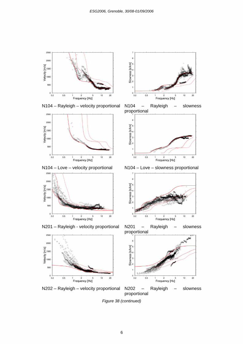
ESG2006, Grenoble, 30/08-01/09/2006

6

N104 – Rayleigh – velocity proportional

N104 – Rayleigh – slowness proportional

N104 – Love – velocity proportional

N104 – Love – slowness proportional

N201 – Rayleigh - velocity proportional

N201 – Rayleigh – slowness proportional

N202 – Rayleigh – velocity proportional

N202 – Rayleigh – slowness proportional

Figure 38 (continued)

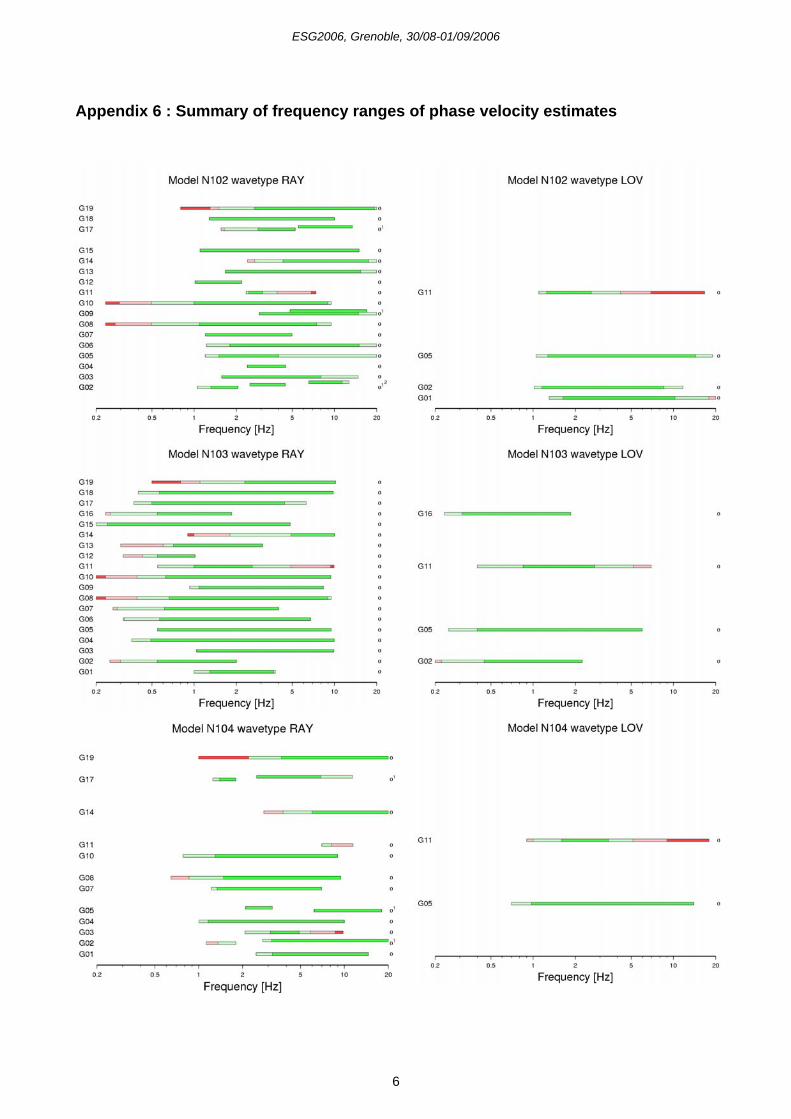
ESG2006, Grenoble, 30/08-01/09/2006

6

Appendix 6 : Summary of frequency ranges of phase velocity estimates

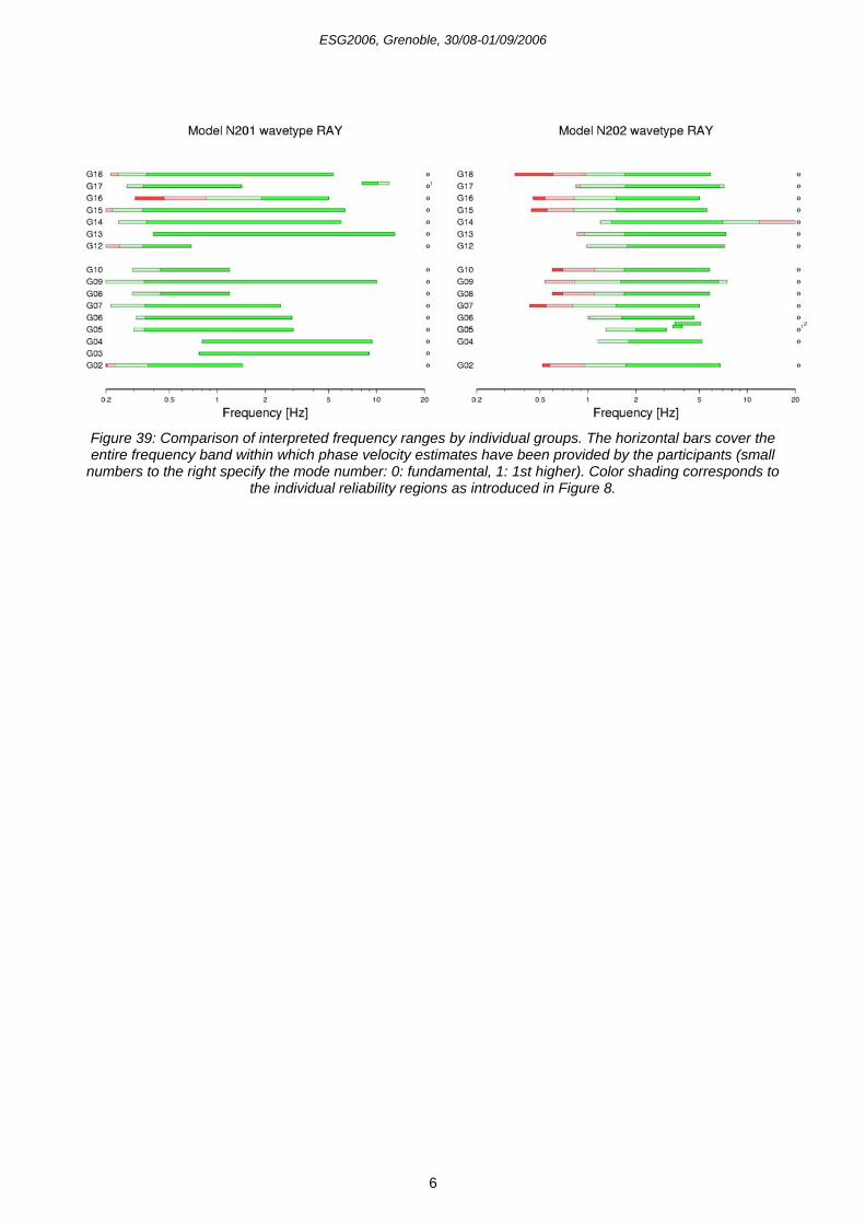
ESG2006, Grenoble, 30/08-01/09/2006

6

Figure 39: Comparison of interpreted frequency ranges by individual groups. The horizontal bars cover the entire frequency band within which phase velocity estimates have been provided by the participants (small

numbers to the right specify the mode number: 0: fundamental, 1: 1st higher). Color shading corresponds to the individual reliability regions as introduced in Figure 8.

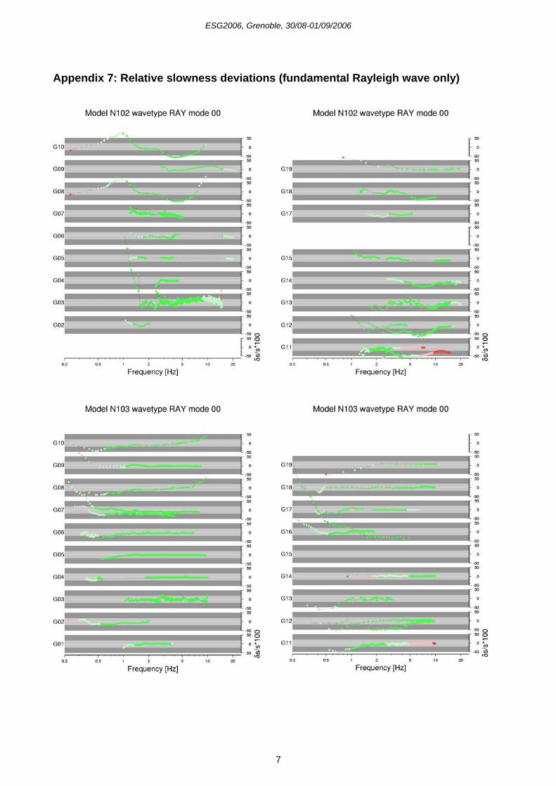
ESG2006, Grenoble, 30/08-01/09/2006

7

Appendix 7: Relative slowness deviations (fundamental Rayleigh wave only)

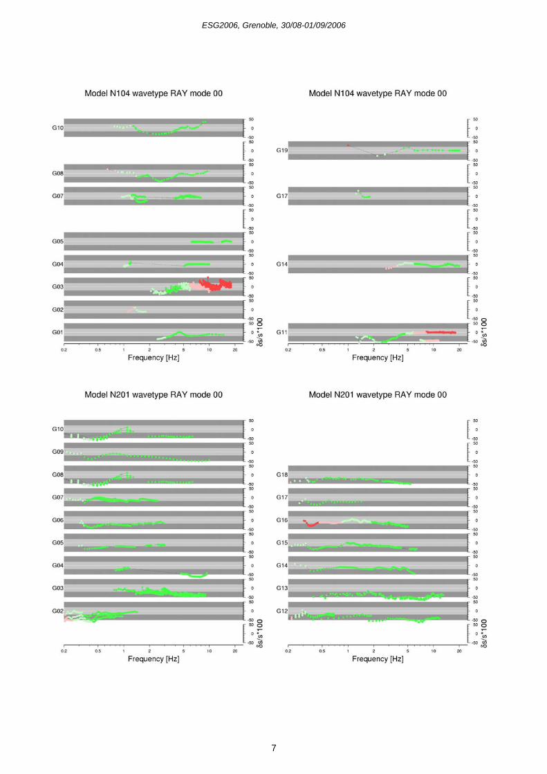
ESG2006, Grenoble, 30/08-01/09/2006

7

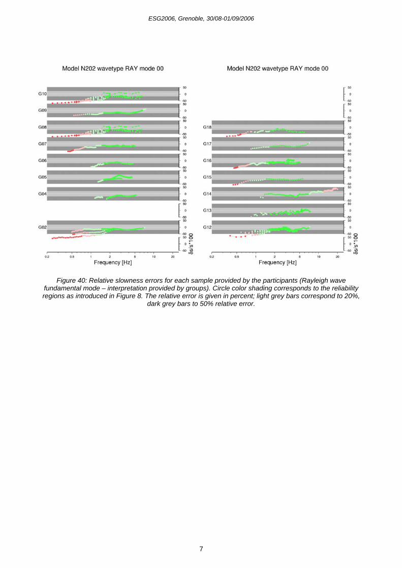
ESG2006, Grenoble, 30/08-01/09/2006

7

Figure 40: Relative slowness errors for each sample provided by the participants (Rayleigh wave fundamental mode – interpretation provided by groups). Circle color shading corresponds to the reliability regions as introduced in Figure 8. The relative error is given in percent; light grey bars correspond to 20%,

dark grey bars to 50% relative error.

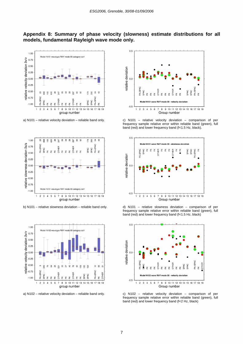
ESG2006, Grenoble, 30/08-01/09/2006

7

Appendix 8: Summary of phase velocity (slowness) estimate distributions for all models, fundamental Rayleigh wave mode only.

a) N101 – relative velocity deviation – reliable band only.

c) N101 – relative velocity deviation – comparison of per frequency sample relative error within reliable band (green), full band (red) and lower frequency band (f<1.5 Hz, black).

b) N101 – relative slowness deviation – reliable band only.

d) N101 – relative slowness deviation – comparison of per frequency sample relative error within reliable band (green), full band (red) and lower frequency band (f<1.5 Hz, black)

a) N102 – relative velocity deviation – reliable band only.

c) N102 – relative velocity deviation – comparison of per frequency sample relative error within reliable band (green), full band (red) and lower frequency band (f<2 Hz, black)

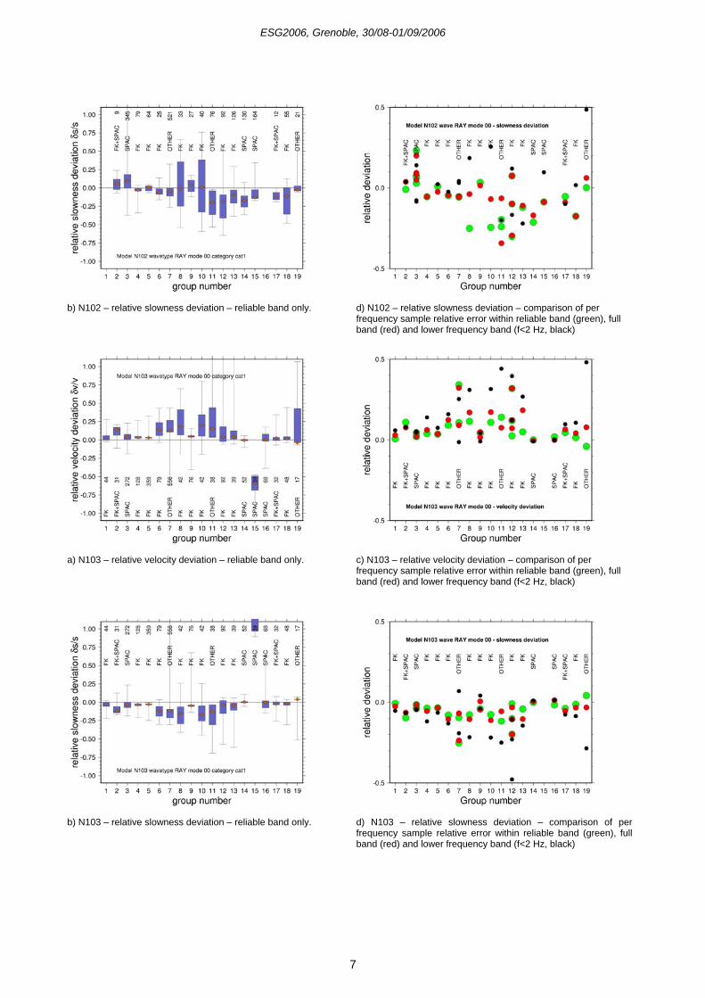
ESG2006, Grenoble, 30/08-01/09/2006

7

b) N102 – relative slowness deviation – reliable band only.

d) N102 – relative slowness deviation – comparison of per frequency sample relative error within reliable band (green), full band (red) and lower frequency band (f<2 Hz, black)

a) N103 – relative velocity deviation – reliable band only.

c) N103 – relative velocity deviation – comparison of per frequency sample relative error within reliable band (green), full band (red) and lower frequency band (f<2 Hz, black)

b) N103 – relative slowness deviation – reliable band only.

d) N103 – relative slowness deviation – comparison of per frequency sample relative error within reliable band (green), full band (red) and lower frequency band (f<2 Hz, black)

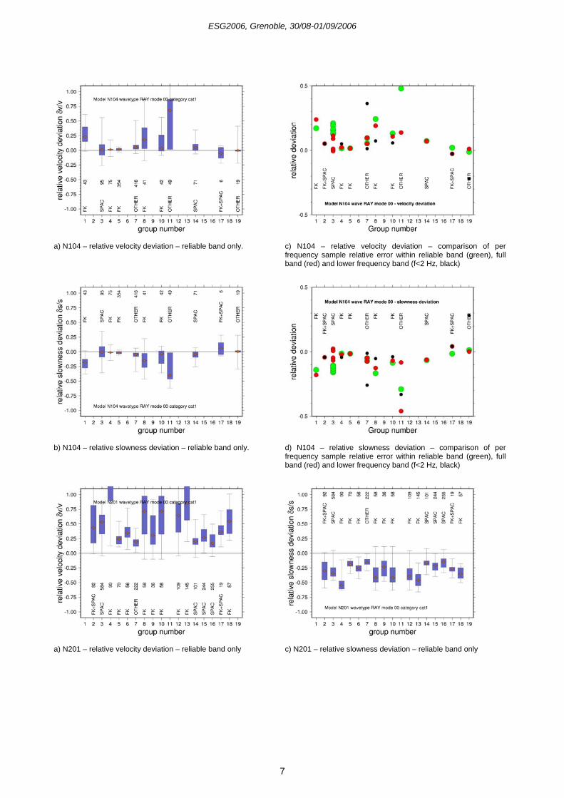
ESG2006, Grenoble, 30/08-01/09/2006

7

a) N104 – relative velocity deviation – reliable band only.

c) N104 – relative velocity deviation – comparison of per frequency sample relative error within reliable band (green), full band (red) and lower frequency band (f<2 Hz, black)

b) N104 – relative slowness deviation – reliable band only.

d) N104 – relative slowness deviation – comparison of per frequency sample relative error within reliable band (green), full band (red) and lower frequency band (f<2 Hz, black)

a) N201 – relative velocity deviation – reliable band only

c) N201 – relative slowness deviation – reliable band only

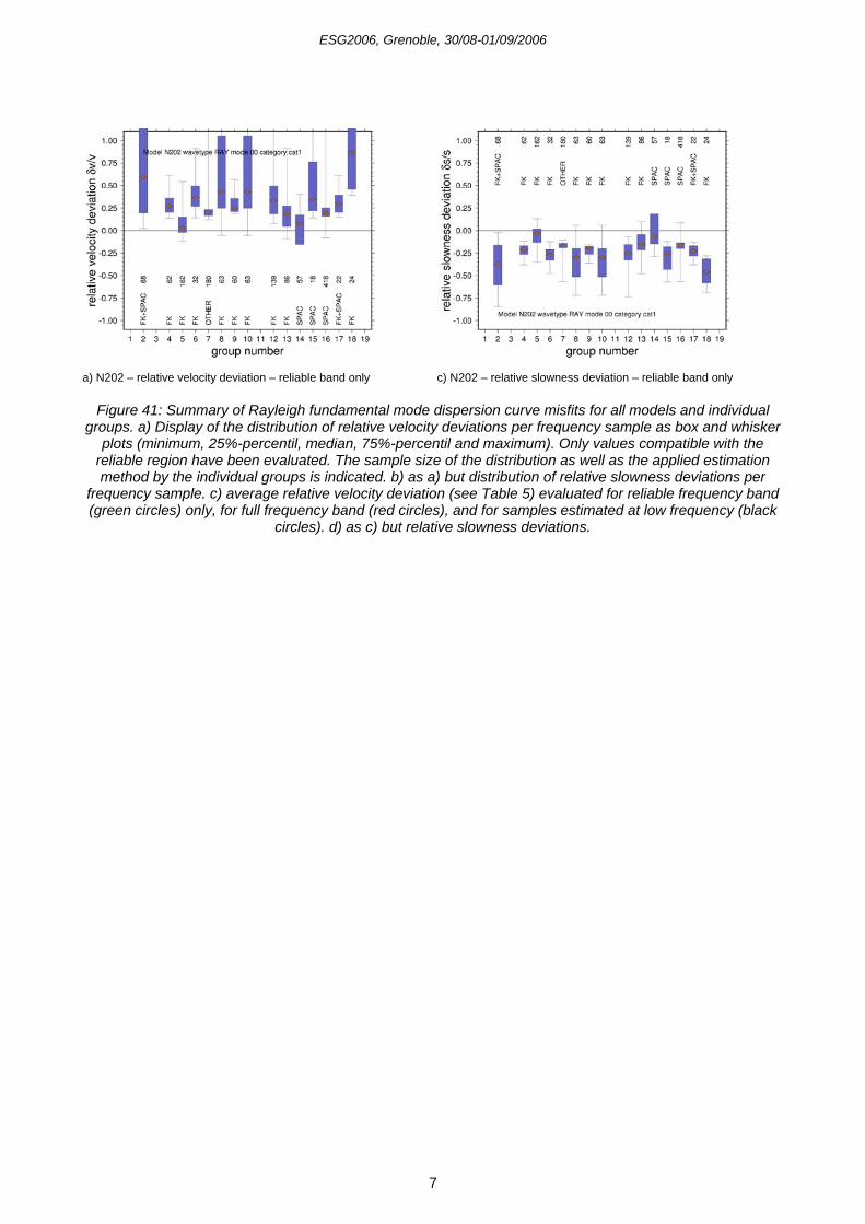
ESG2006, Grenoble, 30/08-01/09/2006

7

a) N202 – relative velocity deviation – reliable band only

c) N202 – relative slowness deviation – reliable band only

Figure 41: Summary of Rayleigh fundamental mode dispersion curve misfits for all models and individual groups. a) Display of the distribution of relative velocity deviations per frequency sample as box and whisker

plots (minimum, 25%-percentil, median, 75%-percentil and maximum). Only values compatible with the reliable region have been evaluated. The sample size of the distribution as well as the applied estimation method by the individual groups is indicated. b) as a) but distribution of relative slowness deviations per

frequency sample. c) average relative velocity deviation (see Table 5) evaluated for reliable frequency band (green circles) only, for full frequency band (red circles), and for samples estimated at low frequency (black

circles). d) as c) but relative slowness deviations.

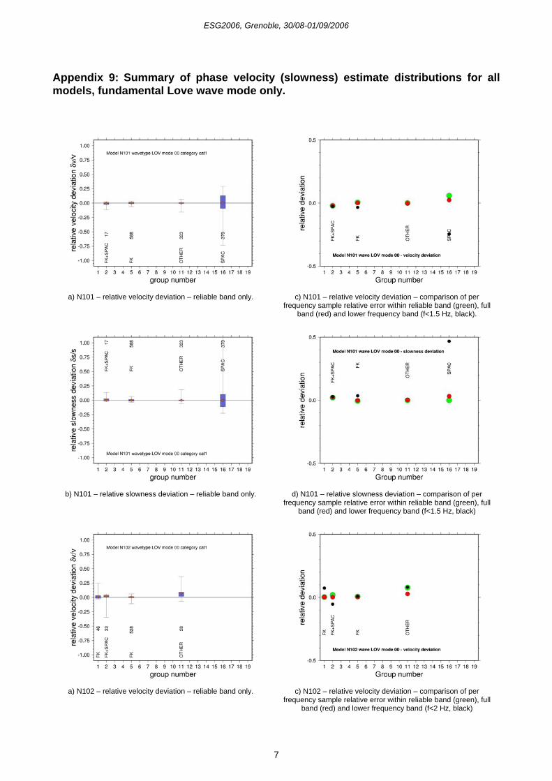
ESG2006, Grenoble, 30/08-01/09/2006

7

Appendix 9: Summary of phase velocity (slowness) estimate distributions for all models, fundamental Love wave mode only.

a) N101 – relative velocity deviation – reliable band only.

c) N101 – relative velocity deviation – comparison of per

frequency sample relative error within reliable band (green), full band (red) and lower frequency band (f<1.5 Hz, black).

b) N101 – relative slowness deviation – reliable band only.

d) N101 – relative slowness deviation – comparison of per

frequency sample relative error within reliable band (green), full band (red) and lower frequency band (f<1.5 Hz, black)

a) N102 – relative velocity deviation – reliable band only.

c) N102 – relative velocity deviation – comparison of per

frequency sample relative error within reliable band (green), full band (red) and lower frequency band (f<2 Hz, black)

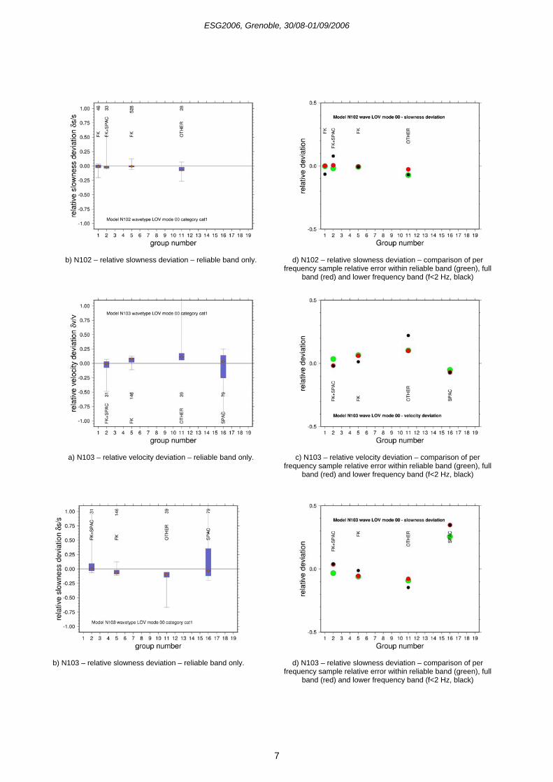
ESG2006, Grenoble, 30/08-01/09/2006

7

b) N102 – relative slowness deviation – reliable band only.

d) N102 – relative slowness deviation – comparison of per

frequency sample relative error within reliable band (green), full band (red) and lower frequency band (f<2 Hz, black)

a) N103 – relative velocity deviation – reliable band only.

c) N103 – relative velocity deviation – comparison of per

frequency sample relative error within reliable band (green), full band (red) and lower frequency band (f<2 Hz, black)

b) N103 – relative slowness deviation – reliable band only.

d) N103 – relative slowness deviation – comparison of per

frequency sample relative error within reliable band (green), full band (red) and lower frequency band (f<2 Hz, black)

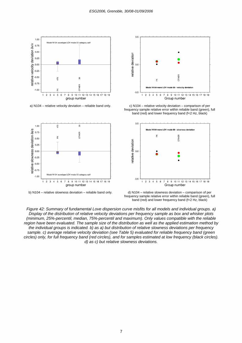
ESG2006, Grenoble, 30/08-01/09/2006

7

a) N104 – relative velocity deviation – reliable band only.

c) N104 – relative velocity deviation – comparison of per

frequency sample relative error within reliable band (green), full band (red) and lower frequency band (f<2 Hz, black)

b) N104 – relative slowness deviation – reliable band only.

d) N104 – relative slowness deviation – comparison of per

frequency sample relative error within reliable band (green), full band (red) and lower frequency band (f<2 Hz, black)

Figure 42: Summary of fundamental Love dispersion curve misfits for all models and individual groups. a) Display of the distribution of relative velocity deviations per frequency sample as box and whisker plots

(minimum, 25%-percentil, median, 75%-percentil and maximum). Only values compatible with the reliable region have been evaluated. The sample size of the distribution as well as the applied estimation method by

the individual groups is indicated. b) as a) but distribution of relative slowness deviations per frequency sample. c) average relative velocity deviation (see Table 5) evaluated for reliable frequency band (green

circles) only, for full frequency band (red circles), and for samples estimated at low frequency (black circles). d) as c) but relative slowness deviations.

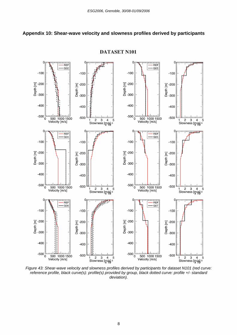
ESG2006, Grenoble, 30/08-01/09/2006

8

Appendix 10: Shear-wave velocity and slowness profiles derived by participants

Figure 43: Shear-wave velocity and slowness profiles derived by participants for dataset N101 (red curve:

reference profile, black curve(s): profile(s) provided by group, black dotted curve: profile +/- standard deviation).

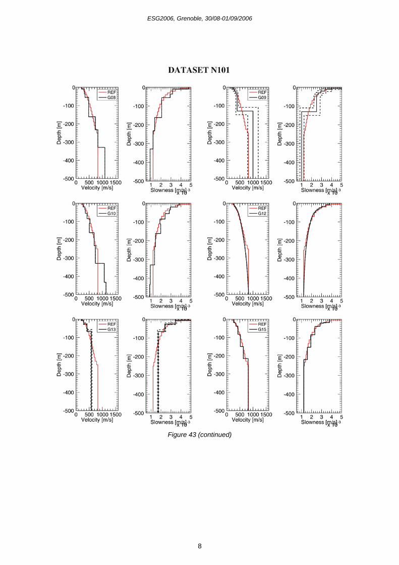
ESG2006, Grenoble, 30/08-01/09/2006

8

Figure 43 (continued)

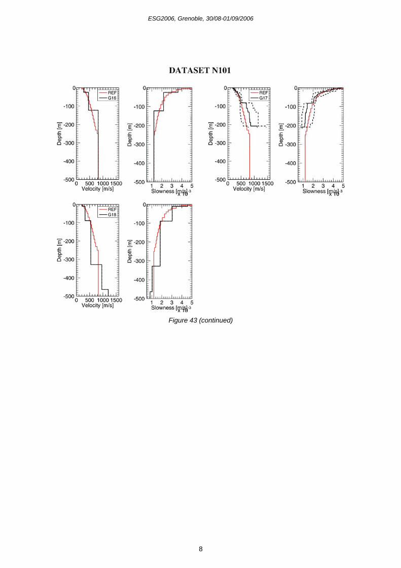
ESG2006, Grenoble, 30/08-01/09/2006

8

Figure 43 (continued)

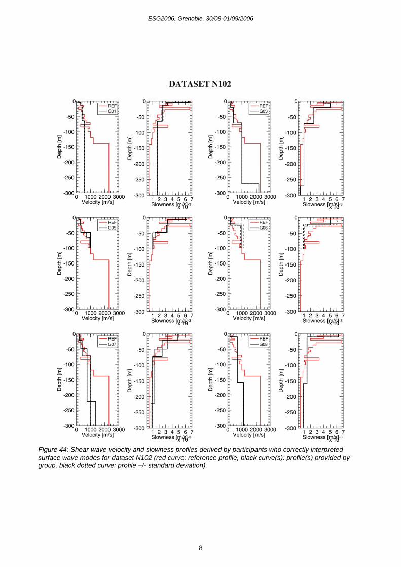
ESG2006, Grenoble, 30/08-01/09/2006

8

Figure 44: Shear-wave velocity and slowness profiles derived by participants who correctly interpreted surface wave modes for dataset N102 (red curve: reference profile, black curve(s): profile(s) provided by group, black dotted curve: profile +/- standard deviation).

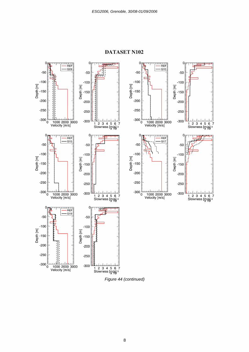
ESG2006, Grenoble, 30/08-01/09/2006

8

Figure 44 (continued)

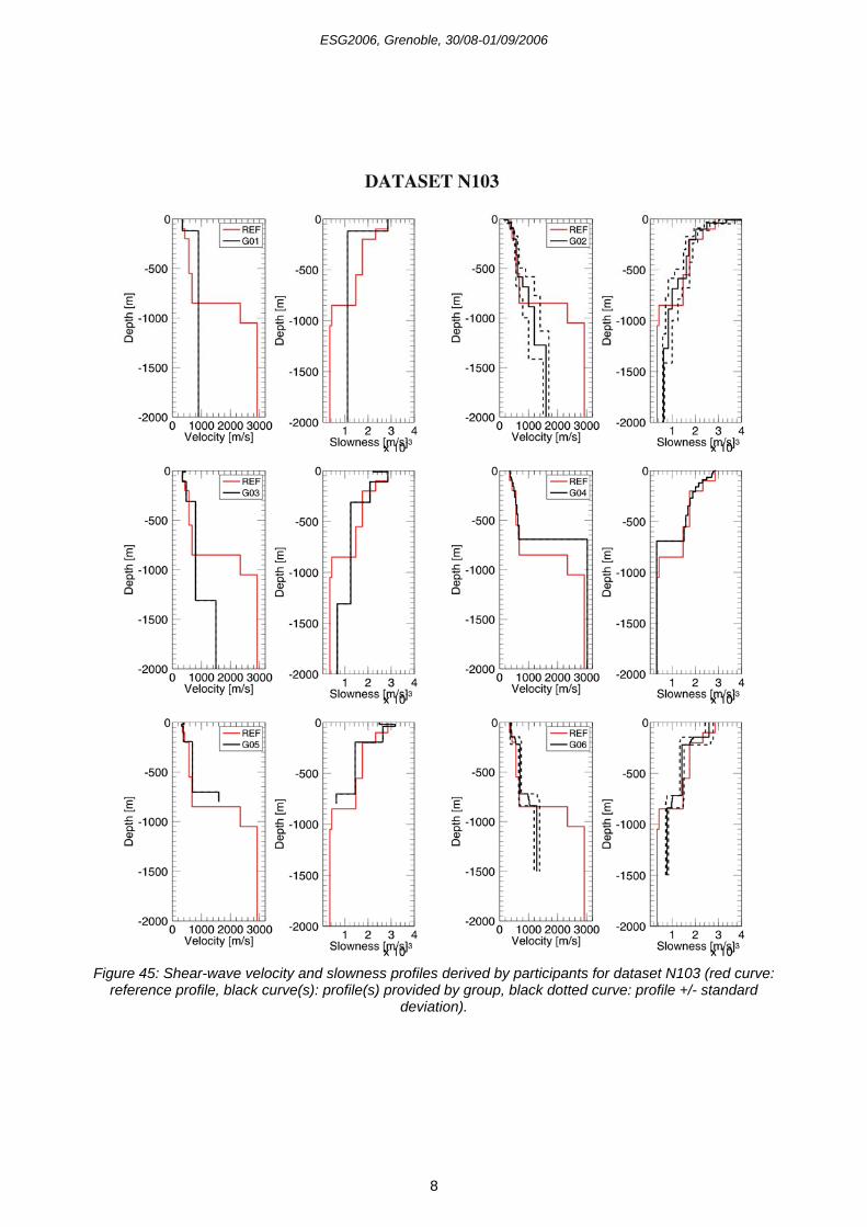
ESG2006, Grenoble, 30/08-01/09/2006

8

Figure 45: Shear-wave velocity and slowness profiles derived by participants for dataset N103 (red curve:

reference profile, black curve(s): profile(s) provided by group, black dotted curve: profile +/- standard deviation).

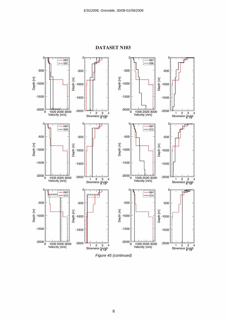
ESG2006, Grenoble, 30/08-01/09/2006

8

Figure 45 (continued)

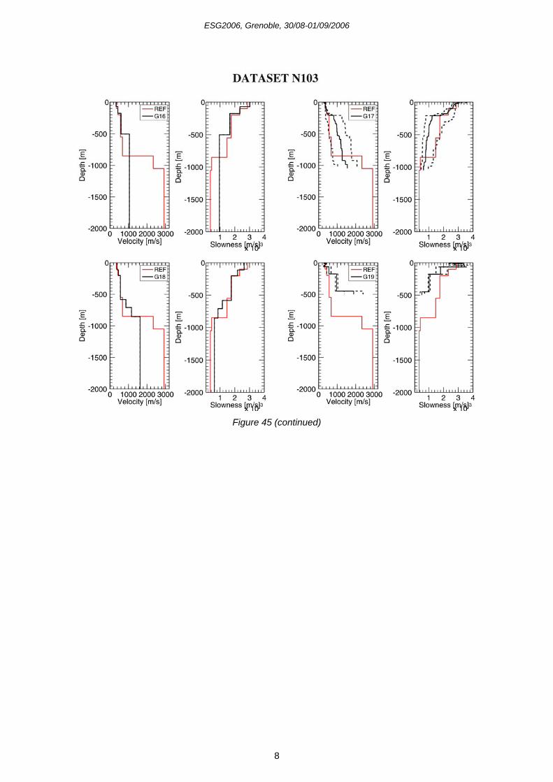
ESG2006, Grenoble, 30/08-01/09/2006

8

Figure 45 (continued)

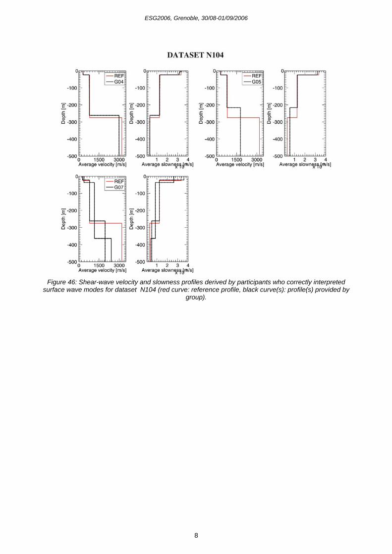
ESG2006, Grenoble, 30/08-01/09/2006

8

Figure 46: Shear-wave velocity and slowness profiles derived by participants who correctly interpreted

surface wave modes for dataset N104 (red curve: reference profile, black curve(s): profile(s) provided by group).

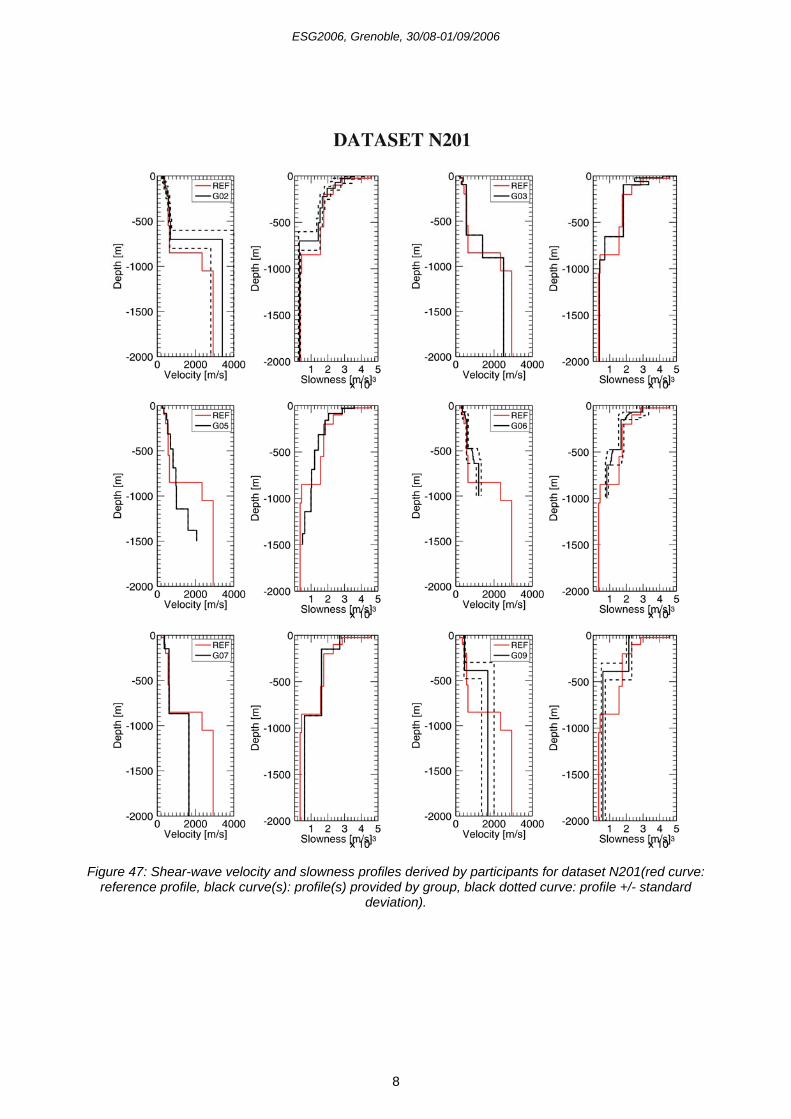
ESG2006, Grenoble, 30/08-01/09/2006

8

Figure 47: Shear-wave velocity and slowness profiles derived by participants for dataset N201(red curve: reference profile, black curve(s): profile(s) provided by group, black dotted curve: profile +/- standard

deviation).

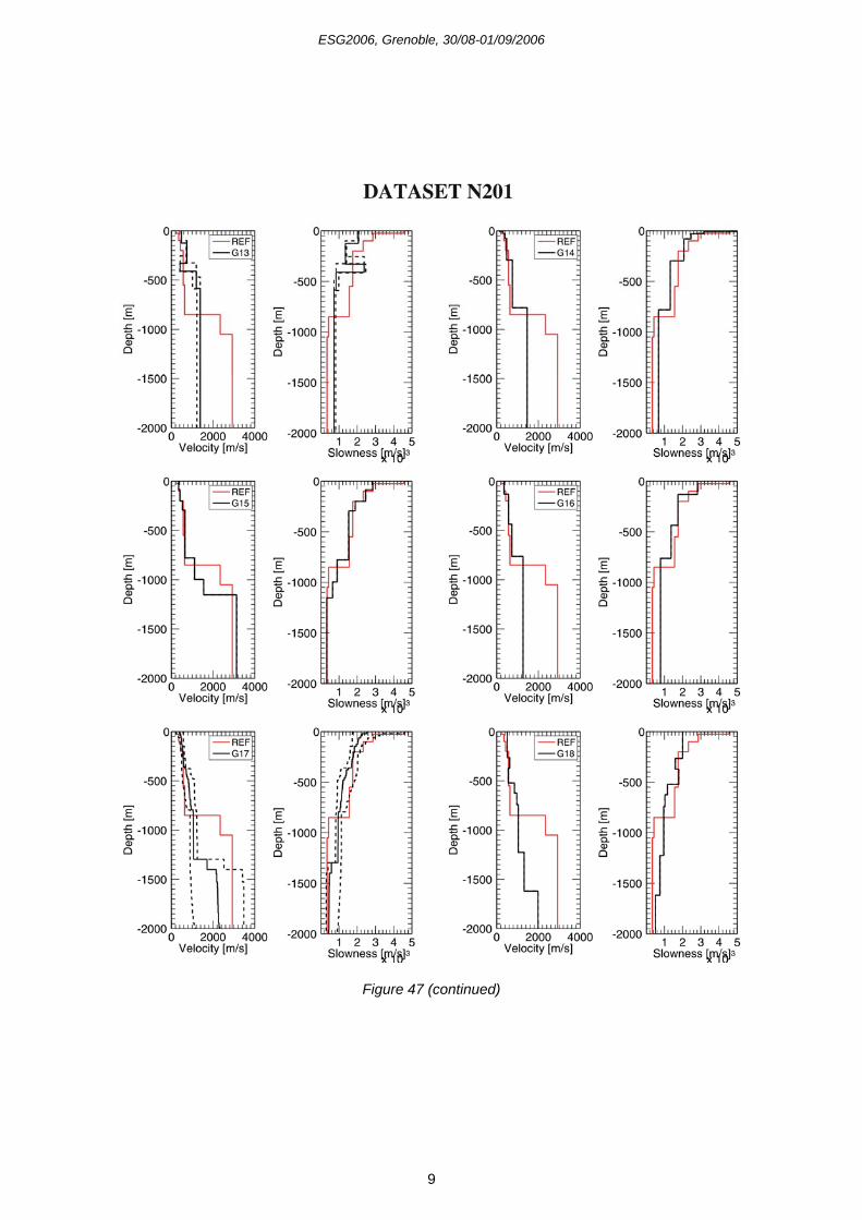
ESG2006, Grenoble, 30/08-01/09/2006

9

Figure 47 (continued)

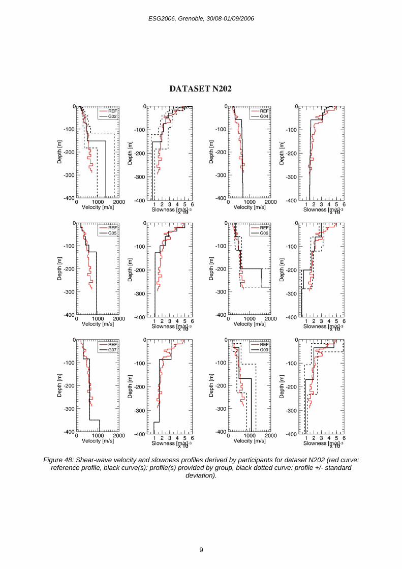
ESG2006, Grenoble, 30/08-01/09/2006

9

Figure 48: Shear-wave velocity and slowness profiles derived by participants for dataset N202 (red curve: reference profile, black curve(s): profile(s) provided by group, black dotted curve: profile +/- standard

deviation).

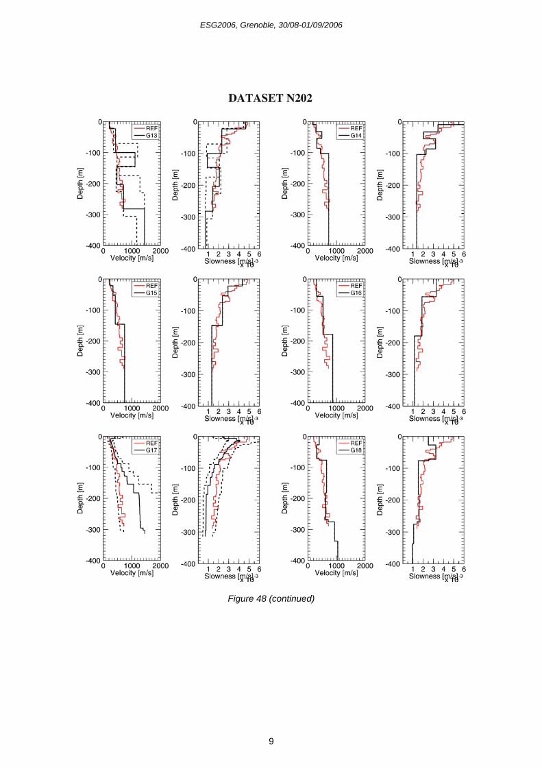
ESG2006, Grenoble, 30/08-01/09/2006

9

Figure 48 (continued)