derek vadala - training brussels
TRANSCRIPT

Managing
RAIDon
LINUXDerek Vadala
Beijing • Cambridge • Farnham • Köln • Paris • Sebastopol • Taipei • Tokyo

Managing RAID on Linuxby Derek Vadala
Copyright © 2003 O’Reilly & Associates, Inc. All rights reserved.Printed in the United States of America.
Published by O’Reilly & Associates, Inc., 1005 Gravenstein Highway North, Sebastopol, CA95472.
O’Reilly & Associates books may be purchased for educational, business, or sales promotionaluse. Online editions are also available for most titles (safari.oreilly.com). For more information,contact our corporate/institutional sales department: (800) 998-9938 or [email protected].
Editor: Andy Oram
Production Editor: Claire Cloutier
Cover Designer: Emma Colby
Interior Designer: David Futato
Printing History:
December 2002: First Edition.
Nutshell Handbook, the Nutshell Handbook logo, and the O’Reilly logo are registeredtrademarks of O’Reilly & Associates, Inc. Many of the designations used by manufacturers andsellers to distinguish their products are claimed as trademarks. Where those designations appearin this book, and O’Reilly & Associates, Inc. was aware of a trademark claim, the designationshave been printed in caps or initial caps. The association between the image of a logjam and thetopic of RAID on Linux is a trademark of O’Reilly & Associates, Inc.
While every precaution has been taken in the preparation of this book, the publisher and authorassume no responsibility for errors or omissions, or for damages resulting from the use of theinformation contained herein.
ISBN: 1-56592-730-3
[M]

v
Table of Contents
Preface . . . . . . . . . . . . . . . . . . . . . . . . . . . . . . . . . . . . . . . . . . . . . . . . . . . . . . . . . . . . . . . . vii
1. Introduction . . . . . . . . . . . . . . . . . . . . . . . . . . . . . . . . . . . . . . . . . . . . . . . . . . . . . . . 1RAID Terminology 3The RAID Levels: An Overview 6RAID on Linux 8Hardware Versus Software 10
2. Planning and Architecture . . . . . . . . . . . . . . . . . . . . . . . . . . . . . . . . . . . . . . . . . . 11Hardware or Software? 11The RAID Levels: In Depth 17RAID Case Studies: What Should I Choose? 28Disk Failures 31Hardware Considerations 32Making Sense of It All 56
3. Getting Started: Building a Software RAID . . . . . . . . . . . . . . . . . . . . . . . . . . . . 59Kernel Configuration 60Working with Software RAID 70Creating an Array 81The Next Step 105
4. Software RAID Reference . . . . . . . . . . . . . . . . . . . . . . . . . . . . . . . . . . . . . . . . . . 106Kernel Options 106md Block Special Files 109/proc and Software RAID 109raidtools 114mdadm 129

vi | Table of Contents
5. Hardware RAID . . . . . . . . . . . . . . . . . . . . . . . . . . . . . . . . . . . . . . . . . . . . . . . . . . . 145Choosing a RAID Controller 145Preparing Controllers and Disks 148General Configuration Issues 150Mylex 155Adaptec 167Promise Technology 1743ware Escalade ATA RAID Controller 181LSI Logic (MegaRAID) 184
6. Filesystems . . . . . . . . . . . . . . . . . . . . . . . . . . . . . . . . . . . . . . . . . . . . . . . . . . . . . . 187Basic Filesystem Concepts 188The Linux Virtual Filesystem (VFS) 191ext2 192ext3 Extensions for the ext2 Filesystem 197ReiserFS 201IBM JFS 207SGI XFS 210
7. Performance, Tuning, and Maintenance . . . . . . . . . . . . . . . . . . . . . . . . . . . . . 214Monitoring RAID Devices 214Managing Disk Failures 216Configuring Hard Disk Parameters 221Performance Testing 227Booting with Software RAID 227
A. Additional Resources . . . . . . . . . . . . . . . . . . . . . . . . . . . . . . . . . . . . . . . . . . . . . . 233
B. Hardware RAID Controller Vendors . . . . . . . . . . . . . . . . . . . . . . . . . . . . . . . . . . 236
Index . . . . . . . . . . . . . . . . . . . . . . . . . . . . . . . . . . . . . . . . . . . . . . . . . . . . . . . . . . . . . . . . . 237

This is the Title of the Book, eMatter EditionCopyright © 2008 O’Reilly & Associates, Inc. All rights reserved.
vii
Preface
Linux has come a long way in the last decade. No longer relegated to the world ofhobbyists and developers, Linux is ubiquitous and is quickly taking hold of enter-prise and high-performance computing. Established corporations such as IBM,Hewlett-Packard, and Sun Microsystems have embraced Linux. Linux is now used toproduce blockbuster motion pictures, create real-time models of worldwide weatherpatterns, and aid in scientific and medical research. Linux is even used on the Inter-national Space Station.
Linux has accomplished this because of a vast, and seemingly tireless, network ofdevelopers, documenters, and evangelists who share the common mantra that soft-ware should be reliable, efficient, and secure as well as free. The hard work of theseindividuals has propelled Linux into the mainstream. Their focus on technologiesthat allow Linux to compete with traditional operating systems certainly accounts fora large part of the success of Linux.
This book focuses on using one of those technologies: RAID, also known as aRedundant Array of Inexpensive Disks. As you will find out, RAID allows individu-als and organizations to get more out of their hardware by increasing the perfor-mance and reliability of their data. RAID is but one component of what makes Linuxa competitive platform.
Overview of the BookHere is a brief overview of the contents of this book.
Chapter 1, Introduction, provides a quick overview of RAID on Linux, including itsevolution and future direction. The chapter briefly outlines the RAID levels and iden-tifies which are available under Linux through hardware or software.
Chapter 2, Planning and Architecture, helps you determine what type of RAID is bestsuited for your needs. The chapter focuses on the differences between hardware andsoftware RAIDs and discusses which is the best choice, depending on your budget

This is the Title of the Book, eMatter EditionCopyright © 2008 O’Reilly & Associates, Inc. All rights reserved.
viii | Preface
and long- and short-term goals. Also included is a discussion of PC hardware rele-vant to building a RAID system: disk protocols, buses, hard drives, I/O channels,cable types and lengths, and cases.
If you decide on a software RAID, then Chapter 3, Getting Started: Building a Soft-ware RAID, outlines the necessary steps in getting your first array online.
Chapter 4, Software RAID Reference, contains all the command-line references forthe RAID utilities available under Linux. It also covers the RAID kernel parametersand commands related to array and disk management.
Chapter 5, Hardware RAID, covers RAID controllers for Linux. Chapter 5 also cov-ers some widely available disk controllers and discusses driver availability, support,and online array management.
Chapter 6, Filesystems, offers a roundup of the journaling filesystems available forLinux, including ext3, IBM’s JFS, ReiserFS, and Silicon Graphics’s XFS. The chaptercovers installation and also offers some performance tuning tips.
Chapter 7, Performance, Tuning, and Maintenance, covers a range of topics thatinclude monitoring RAID devices, tuning hard disks, and booting from softwareRAID.
Appendix A, Additional Resources, lists online resources, mailing lists, and addi-tional reading.
Appendix B, Hardware RAID Controller Vendors, offers information about RAIDvendors.
A Note About ArchitectureIn the interest of appealing to the widest audience, this book covers i386-based sys-tems. Software RAID does work under other architectures, such as SPARC, and Iencourage you to use them. Support for hardware RAID controllers varies betweenarchitectures, so it’s best to contact vendors and confirm hardware compatibilitybefore making any purchases.
KernelsUsing RAID on Linux involves reconfiguring and modifying the Linux kernel. In gen-eral, I prefer to use monolithic kernels instead of modules, whenever possible. Whilekernel modules are quite useful for home desktop systems and notebooks, theyaren’t the best choice for servers and production systems. The choice between thetwo types of kernel is ultimately up to the user. Many users prefer modules to stati-cally compiled kernel subsystems.

This is the Title of the Book, eMatter EditionCopyright © 2008 O’Reilly & Associates, Inc. All rights reserved.
Preface | ix
In order to maintain consistency, I had to settle on specific kernels that are used inthe examples found throughout this book. It’s inevitable that between the time ofthis writing and the release of the book, newer kernels will become available. Thisshould not pose any problem for users working with newer kernels. This book useskernels 2.4.18, 2.2.20, and 2.0.39, and focuses specifically on the 2.4 kernel.
LILOThroughout this book, I focus on LILO when discussing boot loaders. I know thatthere are many other options available (GRUB, for example), but LILO has workedreliably with Linux’s RAID capabilities, and some of the newer choices are not quitecompatible yet.
PromptsThere are a number of command output listings throughout this book. The com-mands in these sections start with a prompt (either $ or #) that indicates whether thecommand should be executed by a normal user or whether it should be run as root.
$ less /etc/raidtab# vi /etc/raidtab
For example, in the preceding code, the $ prompt indicates that the first commandcan be run as a normal user. By default, any user can view, but not modify, the file/etc/raidtab. To edit that file, however, you need root access (as the # promptdenotes).
Conventions Used in This BookThe following typographical conventions are used in this book.
ItalicUsed for file and directory names, programs, commands, command-line options,hostnames, usernames, machine names, email addresses, pathnames, URLs, andnew terms.
Constant widthUsed for variables, keywords, values, options, and IDs. Also used in examples toshow the contents of files or the output from commands.
Constant width italicUsed for text that the user is to replace with an actual value.

This is the Title of the Book, eMatter EditionCopyright © 2008 O’Reilly & Associates, Inc. All rights reserved.
x | Preface
These icons signify a tip, suggestion, or general note.
These icons indicate a warning or caution.
Comments and QuestionsPlease address comments and questions concerning this book to the publisher:
O’Reilly & Associates, Inc.1005 Gravenstein Highway NorthSebastopol, CA 95472(800) 998-9938 (in the U.S. or Canada)(707) 829-0515 (international/local)(707) 829-0104 (fax)
To comment or ask technical questions about this book, send email to:
O’Reilly has a web site for this book, where they’ll list examples, errata, and anyplans for future editions. The site also includes a link to a forum where you can dis-cuss the book with the author and other readers. You can access this site at:
http://www.oreilly.com/catalog/mraidlinux/
For more information about books, conferences, Resource Centers, and the O’ReillyNetwork, see the O’Reilly web site at:
http://www.oreilly.com
AcknowledgmentsMany people helped with the writing of this book, but the greatest credit is owed toAndy Oram, my editor. It was his early interest in my original proposal that startedthis project, and his suggestions, criticism, and raw editorial work turned this textfrom a draft into an O’Reilly book. I’m also indebted to many people at O’Reilly, forall their hard work on the numerous tasks involved in producing a book.
Neil Brown, Nick Moffitt, Jakob Oestergaard, and Levy Vargas reviewed the finaldraft for technical errors and provided me with essential feedback. Their insight andexpertise helped make this book stronger. Many others helped review various bits of
This is the Title of the Book, eMatter EditionCopyright © 2008 O’Reilly & Associates, Inc. All rights reserved.
Preface | xi
material along the way, including Joel Becker, Martin Bene, Danny Cox, Jim Ford,Corin Hartland-Swann, Dan Jones, Eyal Lebedinsky, Greg Lehey, Ingo Molnar, andBenjamin Turner.
Thanks to all the filesystem developers who offered me feedback on Chapter 6:Stephen C. Tweedie, Seth Mos, Steve Lord, Steve Best, Theodore Ts’o, Vladimir V.Saveliev, and Hans Reiser. My appreciation also goes out to all the vendors who pro-vided me with software, equipment, and comments: Thomas Bayens, Chin-TienChu, and Thomas Hall at IBM; Angelina Lu and Deanna Bonds at Adaptec; CraigLyons and Daron Keith at Promise; James Evans at LSI Logic; Pete Kisich, KathleenPaulus, and Adam Radford at 3ware; Joey Lai at Highpoint Technologies; MathildeKraskovetz at Mandrake; and Harshit Mehta at SuSE.
Thanks to my family and friends, who provided support and countless favors while Iwas writing this book, especially Dallas Wisehaupt, Philippe Stephan, StephenFisher, Trevor Noonan, Carolyn Keddy, Erynne Simpson, David Perry, BenjaminRichards, Matthew Williams, Peter Pacheco, Eric Bronnimann, Al Lenderink, BenFeltz, and Erich Bechtel.
I owe special thanks to Craig Newmark, Jim Buckmaster, Jeff Green, and the entirestaff of Craigslist.org for graciously providing me with office space and Internetaccess during my many excursions to San Francisco. Their hospitality directlyresulted in the writing of Chapter 2. And finally, thanks especially to Eric Scheide,who encouraged me to write the original proposal for this book, gave me my first jobas a Unix system administrator, and didn’t argue as I slowly retired Ultrix and Solarismachines in favor of Linux.

This is the Title of the Book, eMatter EditionCopyright © 2008 O’Reilly & Associates, Inc. All rights reserved.
1
Chapter 1 CHAPTER 1
Introduction
Every system administrator sooner or later realizes that the most elusive foe in sus-taining reliable system performance is bandwidth. On one hand, network connectiv-ity provides a crucial connection to the outside world through which your serversdeliver data to users. This type of bandwidth, and its associated issues, is well docu-mented and well studied by virtually all system and network administrators. It is atthe forefront of modern computing, and the topic most often addressed by both non-technical managers and the mainstream media. A multitude of software and docu-mentation has been written to address network and bandwidth issues. Most adminis-trators, however, don’t realize that similar bandwidth problems exist at the bus levelin each system you manage. Unfortunately, this internal data transfer bottleneck ismore sparsely documented than its network counterpart. Because of its second stagecoverage, many administrators, users, and managers are left with often perplexingperformance issues.
Although we tend to think of computers as entirely electronic, they still rely on mov-ing parts. Hard drives, for example, contain plates and mechanical arms that are sub-ject to the constraints of the physical world we inhabit. Introducing moving partsinto a digital computer creates an inherent bottleneck. So even though disk transferspeeds have risen steadily in the past two decades, disks are still an inherently slowcomponent in modern computer systems. A high-performance hard disk might beable to achieve a throughput of around 30 MB per second. But that rate is still morethan a dozen times slower than the speed of a typical motherboard—and the mother-board isn’t even the fastest part of the computer.
There is a solution to this I/O gap that does not include redefining the laws of phys-ics. Systems can alleviate it by distributing the controllers’ and buses’ loads acrossmultiple, identical parts. The trick is doing it in a way that can let the computer dealseamlessly with the complex arrangement of data as if it were one straightforwarddisk. In essence, by increasing the number of moving parts, we can decrease the bot-tleneck. RAID (Redundant Array of Independent Disks) technology attempts to recon-cile this gap by implementing this practical, yet simple, method for swift, invisibledata access.

This is the Title of the Book, eMatter EditionCopyright © 2008 O’Reilly & Associates, Inc. All rights reserved.
2 | Chapter 1: Introduction
Simply put, RAID is a method by which many independent disks attached to a com-puter can be made, from the perspective of users and applications, to appear as a sin-gle disk. This arrangement has several implications.
• Performance can be dramatically improved because the bottleneck of using a sin-gle disk for all I/O is spread across more than one disk.
• Larger storage capacities can be achieved, since you are using multiple disksinstead of a single disk.
• Specific disks can be used to transparently store data that can then be used tosurvive a disk failure.
RAID allows systems to perform traditionally slow tasks in parallel, increasing per-formance. It also hides the complexities of mapping data across multiple hard disksby adding a layer of indirection between users and hardware.
RAID can be achieved in one of two ways. Software RAID uses the computer’s CPUto carry out RAID operations. Hardware RAID uses specialized processors, on diskcontrollers, to manage the disks. The resulting disk set, colloquially called an array,can provide various improvements in performance and reliability, depending on itsimplementation.
The term RAID was coined at Berkeley in 1988 by David A. Patterson, Garth A. Gib-son, and Randy H. Katz in their paper, “A Case for Redundant Arrays of Inexpen-sive Disks (RAID).” This and subsequent articles on RAID have come to be calledthe “Berkeley Papers.” People started to change the “I” in RAID from “inexpensive”to “independent” when they realized, first, that disks were getting so cheap that any-one could afford whatever they needed, and second, that RAID was solving impor-tant problems faced by many computing sites, whether or not cost was an issue.Today, the disk storage playing field has leveled. Large disks have become affordablefor both small companies and consumers. Giant magnetic spindles have been all buteliminated, making even the largest-drives (in terms of capacity) usable on the desk-top. Therefore the evolution of the acronym reflects the definition of RAID today:several independent drives operating in unison. However, the two meanings of theacronym are often used interchangeably.
RAID began as a response to the gap between I/O and processing power. Patterson,Gibson, and Katz saw that while there would continue to be exponential growth inCPU speed and memory capacity, disk performance was achieving only linearincreases and would continue to take this growth curve for the foreseeable future.The Berkeley Papers sought to attack the I/O problem by implementing systems thatno longer relied on a Single Large Expensive Disk (SLED), but rather, concatenatedmany smaller disks that could be accessed by operating systems and applications as asingle disk.

This is the Title of the Book, eMatter EditionCopyright © 2008 O’Reilly & Associates, Inc. All rights reserved.
RAID Terminology | 3
This approach helps to solve many different problems facing many different organi-zations. For example, some organizations might need to deal with data such as news-group postings, which are of relatively low importance, but require an extremelylarge amount of storage. These organizations will realize that a single hard drive isgrossly inadequate for their storage needs and that manually organizing data is afutile effort. Other companies might work with small amounts of vitally importantdata, in a situation in which downtime or data loss would be catastrophic to theirbusiness. RAID, because of its robust and varying implementations, can scale tomeet the needs of both these types of organizations, and many others.
RAID TerminologyOne of the most confusing parts of system administration is its terminology. Misno-mers often obscure simple topics, making it hard to search for documentation andeven harder to locate relevant software. This has unfortunately been the case withRAID on Linux, but Linux isn’t specifically to blame. Since RAID began as an openspecification that was quickly adopted and made proprietary by a multitude of value-added resellers and storage manufacturers, it fell victim to mismarketing. For exam-ple, arrays are often referred to as metadevices, logical volumes, or volume groups.All of these terms mean the same thing: a group of drives that behave as one—thatis, a RAID or an array. In the following section, we will introduce various terms usedto describe RAID.
RAID has the ability to survive disk failures and increase overall disk performance.The RAID levels described in the following section each provide a different combina-tion of performance and reliability. The levels that yield the most impressive perfor-mance often sacrifice the ability to survive disk failures and vice versa.
RedundancyRedundancy is a feature that allows an array to survive a disk failure. Not all RAIDlevels support this feature. In fact, although the term RAID is used to describe cer-tain types of non-redundant arrays, these arrays are not, in fact, RAID because theydo not support any data redundancy.
Despite its redundant capabilities, RAID should never be used as areplacement for reliable backups. RAID does not protect your data inthe event of a fire, natural disaster, or user error.

This is the Title of the Book, eMatter EditionCopyright © 2008 O’Reilly & Associates, Inc. All rights reserved.
4 | Chapter 1: Introduction
Mirroring
Two basic forms of redundancy appear throughout the RAID specification. The firstis accomplished with a process called disk mirroring, shown in Figure 1-1. Mirroringreplicates data onto every disk in the array. Each member disk contains the samedata and has an equal role in the array. In the event of a disk failure, data can be readfrom the remaining disks.
Improved read performance is a by-product of disk mirroring. When the array isoperating normally, meaning that no disks have failed, data can be read in parallelfrom each disk in the mirror. The result is that reads can yield a linear performancebased on the number of disks in the array. A two-disk mirror could yield read speedsup to two times that of a single disk. However, in practice, you probably won’t see aread performance increase that’s quite this dramatic. That’s because many other fac-tors, including filesystem performance and data distribution, also affect throughput.But you can still expect read performance that’s better than that of a single disk.
Unfortunately, mirroring also means that data must be written twice—once to eachdisk in the array. The result is slightly slower write performance, compared to that ofa single disk or nonmirroring array.
Parity
Parity algorithms are the other method of redundancy. When data is written to anarray, recovery information is written onto a separate disk, as shown in Figure 1-2. Ifa drive fails, the original data can be reconstructed from the parity information andthe remaining data. You can find more information on how parity redundancy worksin Chapter 2.
Figure 1-1. Disk mirroring writes a copy of all data to each disk.
Figure 1-2. Parity redundancy is accomplished by storing recovery data on specified drives.
Data
Data(Copy)
Disk array
Data(Copy)
Data
Data(B)
Disk array
Data(C)
Data(A)
Recoverydata

This is the Title of the Book, eMatter EditionCopyright © 2008 O’Reilly & Associates, Inc. All rights reserved.
RAID Terminology | 5
Degraded
Degraded describes an array that supports redundancy, but has one or more faileddisks. The array is still operational, but its reliability and, in some cases, its perfor-mance, is diminished. When an array is in degraded mode, an additional disk failureusually indicates data loss, although certain types of arrays can withstand multipledisk failures.
Reconstruction, resynchronization, and recovery
When a failed disk from a degraded array is replaced, a recovery process begins. Theterms reconstruction, resynchronization, recovery, and rebuild are often used inter-changeably to describe this recovery process. During recovery, data is either copiedverbatim to the new disk (if mirroring was used) or reconstructed using the parityinformation provided by the remaining disks (if parity was used). The recovery pro-cess usually puts an additional strain on system resources. Recovery can be auto-mated by both hardware and software, provided that enough hardware (disks) isavailable to repair an array without user intervention.
Whenever a new redundant array is created, an initial recovery process is performed.This process ensures that all disks are synchronized. It is part of normal RAID opera-tions and does not indicate any hardware or software errors.
StripingStriping is a method by which data is spread across multiple disks (see Figure 1-3). Afixed amount of data is written to each disk. The first disk in the array is not reuseduntil an equal amount of data is written to each of the other disks in the array. Thisresults in improved read and write performance, because data is written to more thanone drive at a time. Some arrays that store data in stripes also support redundancythrough disk parity. RAID-0 defines a striped array without redundancy, resulting inextremely fast read and write performance, but no method for surviving a disk fail-ure. Not all types of arrays support striping.
Figure 1-3. Striping improves performance by spreading data across all available disks.
Disk array
Data1
Disk 1
Data5
Data2
Data6
Disk 2
Data3
Disk 3
Data7
Data4
Data8
Disk 4
Data

This is the Title of the Book, eMatter EditionCopyright © 2008 O’Reilly & Associates, Inc. All rights reserved.
6 | Chapter 1: Introduction
Stripe-size versus chunk-size
The stripe-size of an array defines the amount of data written to a group of paralleldisk blocks. Assume you have an array of four disks with a stripe size of 64 KB (acommon default). In this case, 16 KB worth of data is written to each disk (seeFigure 1-4), for a total of 64 KB per stripe. An array’s chunk-size defines the smallestamount of data per write operation that should be written to each individual disk.That means a striping array made up of four disks, with a chunk-size of 64 KB, has astripe-size of 256 KB, because a minimum of 64 KB is written to each componentdisk. Depending on the specific RAID implementation, users may be asked to set astripe-size or a chunk-size. For example, most hardware RAID controllers use astripe-size, while the Linux kernel uses a chunk-size.
The RAID Levels: An OverviewPatterson, Gibson, and Katz realized that different types of systems would inevitablyhave different performance and redundancy requirements. The Berkeley Papers pro-vided specifications for five levels of RAID, offering various compromises betweenperformance and data redundancy. After the publication of the Berkeley Papers,however, the computer industry quickly realized that some of the original levelsfailed to provide a good balance between cost and performance, and thereforeweren’t really worth using.
RAID-2 and RAID-3, for example, quickly became useless. RAID-2 implemented aread/write level error correction code (ECC) that later became a standard firmwarefeature on hard drives. This development left RAID-2 without any advantage inredundancy over other RAID levels. The ECC implementation now required unnec-essary overhead that hurt performance. RAID-3 required that all disks operate inlockstep (all disk spindles are synchronized). This added additional design consider-ations and did not provide any significant advantage over other RAID levels.
RAID has changed a great deal since the Berkeley Papers were written. While someof the original levels are no longer used, the storage industry quickly made additions
Figure 1-4. Stripe-size defines the size of write operations.
64KB Write
Disk array
16KB 16KB 16KB 16KB
Stripe size
Chunk size

This is the Title of the Book, eMatter EditionCopyright © 2008 O’Reilly & Associates, Inc. All rights reserved.
The RAID Levels: An Overview | 7
to the original specification. This book will cover all of the RAID levels available toLinux users, but will not cover obsolete implementations like RAID-2 and RAID-3.Below you will find a concise overview of each RAID level. Chapter 2 covers each ofthe RAID levels in more detail, including hybrid arrays that are built by combiningmultiple RAID levels.
RAID-0: StripingRAID-0 is also known as striping because data is interleaved across all drives in thearray. Each block of data is written in round-robin fashion to array disks until thewrite operation is complete. Data is read in the same fashion. Since data transfer isconstantly shifted to a new disk, bottlenecks associated with reading and writingdata to a single disk are alleviated and performance dramatically improves. Stripingwas not part of the original RAID specification and, technically speaking, is not aRAID because it provides no mechanism for data redundancy. Nonetheless, the con-cept of striping is also found in other RAID levels. For example, RAID-4 and RAID-5(described below) use a combination of striping and recovery algorithms to achieveimprovements in performance while still offering redundancy.
RAID-1: MirroringRAID-1 (mirroring) stores an exact replica of all data on a separate disk or disks. Thispractice provides complete data redundancy in the event of a disk failure. However,because data must be written to disk more than once, there is a write performancehit, which increases as you add disks. On the other hand, read operations can bedone in parallel so that read performance improves (compared to that of a singledisk), depending on the number of disks in the mirror.
RAID-4: Dedicated ParityRAID-4 works similarly to striping. However, a dedicated drive is used to store par-ity information. Every time data is written to an array disk, an algorithm generatesrecovery information that is written to a specially flagged parity drive. In the event ofsingle disk failure, the algorithm can be reversed and missing data can be automati-cally generated, based on the remaining data and the parity information.
RAID-5: Distributed ParityRAID-5 is similar to RAID-4, except that the parity information is spread across alldrives in the array. This helps reduce the bottleneck inherent in writing parity infor-mation to a single drive during each write operation.

This is the Title of the Book, eMatter EditionCopyright © 2008 O’Reilly & Associates, Inc. All rights reserved.
8 | Chapter 1: Introduction
Linear ModeLinear mode, also called append mode, writes data to a single array disk until it isfull. Once the disk is full, data is written to the next disk in the array until all disksare full. This provides an easy way to use disks of different sizes in an array, so thatno space is ever wasted. Like striping, linear mode is not technically a RAID, becauseno redundancy is provided. It was also not present in the original RAID specifica-tion. For clarity, I will use the term linear mode, rather than append mode, through-out the rest of the book.
Disk spanning
The term linear mode is unique to the Linux kernel’s implementation of RAID. Mosthardware RAID vendors use the term disk spanning, or simply spanning, to refer tothis type of end-to-end disk arrangement. The terms disk concatenation or concate-nated disks are also used.
JBOD (Just a Bunch Of Disks)JBOD refers to the single-disk operating mode that many hardware RAID controllerssupport. With JBOD mode, the controller is able to circumvent RAID firmware andtreat a single hard disk as a normal disk controller would. This is useful when youhave disks that you want to configure without RAID support, but that you want toconnect to a RAID controller. If your controller does not support JBOD, then youwould need to use a standard disk controller to connect non-RAID disks, resulting inadditional hardware spending and the use of another expansion slot.
I have seen some instances where the term JBOD is used interchangeably with termslike linear mode, disk spanning, and concatenation. When I use it throughout thisbook, I mean it in the context described here: a standalone disk connected to a RAIDcontroller.
RAID on LinuxIt’s important to understand that when I refer to a RAID array, I’m talking about ablock device and not a filesystem. You could think of the relationship between thetwo much in the same way you might think of the relationship between a house andits foundation. If the foundation is weak, the house will eventually collapse. The file-system, which represents the house in my analogy, is built on top of a block device.Normally, a block device is a single hard disk, but RAID introduces another layer(see Figure 1-5). RAID groups many block devices into a single virtual device.
This means that Linux interacts with an array through a single block device having asingle major and minor number. Physically, the array device points to many differentphysical disks, each with their own major and minor numbers. Programmers might

This is the Title of the Book, eMatter EditionCopyright © 2008 O’Reilly & Associates, Inc. All rights reserved.
RAID on Linux | 9
think of this model the same way they think of an array data type, hence the use ofthe word “array” in the RAID acronym.
Each piece of hardware connected to a Linux system is assigned a major and minornumber. The major number refers to a specific group of hardware (such as smallcomputer systems interface, or SCSI, disks), while the minor uniquely identifies eachinstalled piece of hardware within the group (for example, each individual SCSIdisk). Since RAID is merely an intermediary layer, and because it works just like anyother block device, you can build any type of filesystem on top of it. When workingwith Linux’s RAID implementation, you can even build arrays on top of other arrays,or use other types of storage management like Logical Volume Management (LVM).
The Linux device names for accessing software RAID devices are designated md.While you might assume that md stands for metadevice, that’s incorrect (althoughthe abbreviation is used that way by many people). The md in Linux software RAIDactually refers to the kernel subsystem that handles arrays: the multiple devices driver./dev/md[0-255] represents the default block devices used for accessing softwareRAID on Linux, allowing a total of 256 software RAID devices on a single Linux sys-tem.
RAID under Linux is available as part of the kernel. The kernel supports five differ-ent RAID levels: linear mode, striping (RAID-0), mirroring (RAID-1), RAID-4, andRAID-5. The RAID subsystem can be compiled statically into the kernel or used as aloadable module. Chapter 3 covers software RAID implementation under Linux. Ifyou are already familiar with RAID from an architectural standpoint, you can skipahead to Chapter 3 and start rebuilding your kernel.
With the popularity of Linux increasing daily, many manufacturers have begun torelease Linux drivers for hardware RAID cards and offer full-scale technical supportfor such RAID cards. Many of these companies have gone one step further andreleased drivers that are open source (http://opensource.org). Some companies that
Figure 1-5. Filesystems are built on block devices; RAID introduces an intermediary layer.
ReiserFS ext2 IBMs andJFS XFS ext3
Filesystems
I/O
Software RAID devices (md driver)/dev/mdo, /dev/md1, etc.
I/O
Block devices/dev/sda1, /dev/sdb1, /dev/hda1, etc.

This is the Title of the Book, eMatter EditionCopyright © 2008 O’Reilly & Associates, Inc. All rights reserved.
10 | Chapter 1: Introduction
have not been kind enough to release drivers have still released technical informa-tion about their hardware that has allowed open source developers to write drivers.This growing industry support allows Linux, and open source, to more effectivelycompete with commercial systems and legacy operating systems.
Linux professionals have done considerable work to bring high-performance, opensource filesystems to Linux. These filesystems include IBM’s Journaled File System(JFS), ext3, SGI’s XFS, and ReiserFS. However, improving the performance and reli-ability of a filesystem can be a wasted effort if equal consideration is not given to theblock devices on which these filesystems are built. Likewise, you’d be foolish tospend your time building a reliable, high-performance RAID system without consid-ering the filesystem that you are going to use. In fact, in many cases, limitations offilesystems like ext2 will prevent you from fully realizing the potential of a RAIDdevice. Chapter 6 provides a brief overview of some high-performance filesystems.
Hardware Versus SoftwareAlthough RAID is built directly into the Linux kernel, some users might find itadvantageous to buy custom drive controllers that have built-in RAID capabilities.Some users might even find it worthwhile to purchase custom RAID systems thathave been preconfigured. The choice between using software (kernel-based) or hard-ware (controller-based) RAID or buying a turnkey RAID solution can be difficult, butthis book will help you determine which option is best suited for your needs.

This is the Title of the Book, eMatter EditionCopyright © 2008 O’Reilly & Associates, Inc. All rights reserved.
11
Chapter 2 CHAPTER 2
Planning andArchitecture
Choosing the right RAID solution can be a daunting task. Buzzwords and marketingoften cloud administrators’ understanding of RAID technology. Conflicting informa-tion can cause inexperienced administrators to make mistakes. It is not unnatural tomake mistakes when architecting a complicated system. But unfortunately, dead-lines and financial considerations can make any mistakes catastrophic. I hope thatthis book, and this chapter in particular, will leave you informed enough to make asfew mistakes as possible, so you can maximize both your time and the resources youhave at your disposal. This chapter will help you pick the best RAID solution by firstselecting which RAID level to use and then focusing on the following areas:
• Hardware costs
• Scalability
• Performance and redundancy
Hardware or Software?RAID, like many other computer technologies, is divided into two camps: hardwareand software. Software RAID uses the computer’s CPU to perform RAID operationsand is implemented in the kernel. Hardware RAID uses specialized processors, usu-ally found on disk controllers, to perform array management functions. The choicebetween software and hardware is the first decision you need to make.
Software (Kernel-Managed) RAIDSoftware RAID means that an array is managed by the kernel, rather than by special-ized hardware (see Figure 2-1). The kernel keeps track of how to organize data onmany disks while presenting only a single virtual device to applications. This virtualdevice works just like any normal fixed disk.

This is the Title of the Book, eMatter EditionCopyright © 2008 O’Reilly & Associates, Inc. All rights reserved.
12 | Chapter 2: Planning and Architecture
Software RAID has unfortunately fallen victim to a FUD (fear, uncertainty, doubt)campaign in the system administrator community. I can’t count the number of sys-tem administrators whom I’ve heard completely disparage all forms of softwareRAID, irrespective of platform. Many of these same people have admittedly not usedsoftware RAID in several years, if at all.
Why the stigma? Well, there are a couple of reasons. For one, when software RAIDfirst saw the light of day, computers were still slow and expensive (at least by today’sstandards). Offloading a high-performance task like RAID I/O onto a CPU that waslikely already heavily overused meant that performing fundamental tasks such as fileoperations required a tremendous amount of CPU overhead. So, on heavily satu-rated systems, the simple task of calling the stat* function could be extremely slowwhen compared to systems that didn’t have the additional overhead of managingRAID arrays. But today, even multiprocessor systems are both inexpensive and com-mon. Previously, multiprocessor systems were very expensive and unavailable to typ-ical PC consumers. Today, anyone can build a multiprocessor system usingaffordable PC hardware. This shift in hardware cost and availability makes softwareRAID attractive because Linux runs well on common PC hardware. Thus, in caseswhen a single-processor system isn’t enough, you can cost-effectively add a secondprocessor to augment system performance.
Another big problem was that software RAID implementations were part of propri-etary operating systems. The vendors promoted software RAID as a value-added
Figure 2-1. Software RAID uses the kernel to manage arrays.
* The stat(2) system call reports information about files and is required for many commonplace activities likethe ls command.
Software RAID
Users and applications
Data
CPU
Raw disk blocks
Read Write
Disk controller(No RAID capability)

This is the Title of the Book, eMatter EditionCopyright © 2008 O’Reilly & Associates, Inc. All rights reserved.
Hardware or Software? | 13
incentive for customers who couldn’t afford hardware RAID, but who needed a wayto increase disk performance and add redundancy. The problem here was thatclosed-source implementations, coupled with the fact that software RAID wasn’t apriority in OS development, often left users with buggy and confusing packages.
Linux, on the other hand, has a really good chance to change the negative percep-tions of software RAID. Not only is Linux’s software RAID open source, the inex-pensive hardware that runs Linux finally makes it easy and affordable to buildreliable software RAID systems. Administrators can now build systems that have suf-ficient processing power to deal with day-to-day user tasks and high-performancesystem functions, like RAID, at the same time. Direct access to developers and ahelpful user base doesn’t hurt, either.
If you’re still not convinced that software RAID is worth your time, then don’t fret.There are also plenty of hardware solutions available for Linux.
HardwareHardware RAID means that arrays are managed by specialized disk controllers thatcontain RAID firmware (embedded software). Hardware solutions can appear in sev-eral forms. RAID controller cards that are directly attached to drives work like anynormal PCI disk controller, with the exception that they are able to internally admin-ister arrays. Also available are external storage cabinets that are connected to high-end SCSI controllers or network connections to form a Storage Area Network (SAN).There is one common factor in all these solutions: the operating system accesses onlya single block device because the array itself is hidden and managed by the control-ler.
Large-scale and expensive hardware RAID solutions are typically faster than soft-ware solutions and don’t require additional CPU overhead to manage arrays. ButLinux’s software RAID can generally outperform low-end hardware controllers.That’s partly because, when working with Linux’s software RAID, the CPU is muchfaster than a RAID controller’s onboard processor, and also because Linux’s RAIDcode has had the benefit of optimization through peer review.
The major trade-off you have to make for improved performance is lack of support,although costs will also increase. While hardware RAID cards for Linux have becomemore ubiquitous and affordable, you may not have some things you traditionally getwith Linux. Direct access to developers is one example. Mailing lists for the Linuxkernel and for the RAID subsystem are easily accessible and carefully read by thedevelopers who spend their days working on the code. With some exceptions, youprobably won’t get that level of support from any disk controller vendor—at leastnot without paying extra.
Another trade-off in choosing a hardware-based RAID solution is that it probablywon’t be open source. While many vendors have released cards that are supported

This is the Title of the Book, eMatter EditionCopyright © 2008 O’Reilly & Associates, Inc. All rights reserved.
14 | Chapter 2: Planning and Architecture
under Linux, a lot of them require you to use closed-source components. This meansthat you won’t be able to fix bugs yourself, add new features, or customize the codeto meet your needs. Some manufacturers provide open source drivers while provid-ing only closed-source, binary-only management tools, and vice versa. No vendorsprovide open source firmware. So if there is a problem with the software embeddedon the controller, you are forced to wait for a fix from the vendor—and that couldimpact a data recovery effort! With software RAID, you could write your own patchor pay someone to write one for you straightaway.
RAID controllers
Some disk controllers internally support RAID and can manage disks without thehelp of the CPU (see Figure 2-2). These RAID cards handle all array functions andpresent the array as a standard block device to Linux. Hardware RAID cards usuallycontain an onboard BIOS that provides the management tools for configuring andmaintaining arrays. Software packages that run at the OS level are usually providedas a means of post-installation array management. This allows administrators tomaintain RAID devices without rebooting the system.
While a lot of card manufacturers have recently begun to support Linux, it’s impor-tant to make sure that the card you’re planning to purchase is supported underLinux. Be sure that your manufacturer provides at least a loadable kernel module, or,ideally, open source drivers that can be statically compiled into the kernel. Opensource drivers are always preferred over binary-only kernel modules. If you are stuckusing a binary-only module, you won’t get much support from the Linux commu-nity because without access to source code, it’s quite impossible for them to diag-nose interoperability problems between proprietary drivers and the Linux kernel.Luckily, several vendors either provide open source drivers or have allowed kernel
Figure 2-2. Disk controllers shift the array functions off the CPU, yielding an increase inperformance.
Users and applications
CPU
Data
Hardware RAID
Read Write
RAID controller

This is the Title of the Book, eMatter EditionCopyright © 2008 O’Reilly & Associates, Inc. All rights reserved.
Hardware or Software? | 15
hackers to develop their own. One shining example is Mylex, which sells RAID con-trollers. Their open source drivers are written by Leonard Zubkoff* of DandelionDigital and can be managed through a convenient interface under the /proc filesys-tem. Chapter 5 discusses some of the cards that are currently supported by Linux.
Outboard solutions
The second hardware alternative is a turnkey solution, usually found in outboarddrive enclosures. These enclosures are typically connected to the system through astandard or high-performance SCSI controller. It’s not uncommon for these special-ized systems to support multiple SCSI connections to a single system, and many ofthem even provide directly accessible network storage, using NFS and other proto-cols.
These outboard solutions generally appear to an operating system as a standard SCSIblock device or network mount point (see Figure 2-3) and therefore don’t usuallyrequire any special kernel modules or device drivers to function. These solutions areoften extremely expensive and operate as black box devices, in that they are almostalways proprietary solutions. Outboard RAID boxes are nonetheless highly popularamong organizations that can afford them. They are highly configurable and theirmodular construction provides quick and seamless, although costly, replacementoptions. Companies like EMC and Network Appliance specialize in this arena.
* Leonard Zubkoff was very sadly killed in a helicopter crash on August 29, 2002. I learned of his death abouta week later, as did many in the open source community. I didn’t know Leonard personally. We’d had onlyone email exchange, earlier in the summer of 2002, in which he had graciously agreed to review material Ihad written about the Mylex driver. His site remains operational, but I have created a mirror at http://dandelion.cynicism.com/, which I will maintain indefinitely.
Figure 2-3. Outboard RAID systems are internally managed and connected to a system to whichthey appear as a single hard disk.
Storage cabinet populated withhot-swap drives
DataOn-board RAID controllers
Raw disk blocks Ethernet or direct connectionusing SCSI or Fiber channel

This is the Title of the Book, eMatter EditionCopyright © 2008 O’Reilly & Associates, Inc. All rights reserved.
16 | Chapter 2: Planning and Architecture
If you can afford an outboard RAID system and you think it’s the best solution foryour project, you will find them reliable performers. Do not forget to factor supportcosts into your budget. Outboard systems not only have a high entry cost, but theyare also costly to maintain. You might also consider factoring spare parts into yourbudget, since a system failure could otherwise result in downtime while you are wait-ing for new parts to arrive. In most cases, you will not be able to find replacementparts for an outboard system at local computer stores, and even if they are available,using them will more than likely void your warranty and support contracts.
I hope you will find the architectural discussions later in this chapter helpful whenchoosing a vendor. I’ve compiled a list of organizations that provide hardware RAIDsystems in the Appendix. But I urge you to consider the software solutions discussedthroughout this book. Administrators often spend enormous amounts of money onsolutions that are well in excess of their needs. After reading this book, you may findthat you can accomplish what you set out to do with a lot less money and a littlemore hard work.
Storage Area Network (SAN)
SAN is a relatively new method of storage management, in which various storageplatforms are interconnected on a separate, usually high-speed, network (seeFigure 2-4). The SAN is then connected to local area networks (LANs) throughoutan organization. It is not uncommon for a SAN to be connected to several differentparts of a LAN so that users do not share a single path to the SAN. This prevents anetwork bottleneck and allows better throughput between users and storage sys-tems. Typically, a SAN might also be exposed to satellite offices using wide area net-work (WAN) connections.
Many companies that produce turnkey RAID solutions also offer services for plan-ning and implementing a SAN. In fact, even drive manufacturers such as IBM andWestern Digital, as well as large network and telecommunications companies suchas Lucent and Nortel Networks, now provide SAN solutions.
SAN is very expensive, but is quickly becoming a necessity for large, distributedorganizations. It has become vital in backup strategies for large businesses and willlikely grow significantly over the next decade. SAN is not a replacement for RAID;rather, RAID is at the heart of SAN. A SAN could be comprised of a robotic tapebackup solution and many RAID systems. SAN uses data and storage managementin a world where enormous amounts of data need to be stored, organized, andrecalled at a moment’s notice. A SAN is usually designed and implemented by ven-dors as a top-down solution that is customized for each organization. It is thereforenot discussed further in this book.

This is the Title of the Book, eMatter EditionCopyright © 2008 O’Reilly & Associates, Inc. All rights reserved.
The RAID Levels: In Depth | 17
The RAID Levels: In DepthIt is important to realize that different implementations of RAID are suited to differ-ent applications and the wallets of different organizations. All implementationsrevolve around the basic levels first outlined in the Berkeley Papers. These core lev-els have been further expanded by software developers and hardware manufactur-ers. The RAID levels are not organized hierarchically, although vendors sometimesmarket their products to imply that there is a hierarchical advantage. As discussed inChapter 1, the RAID levels offer varying compromises between performance andredundancy. For example, the fastest level offers no additional reliability when com-pared with a standalone hard disk. Choosing an appropriate level assumes that youhave a good understanding of the needs of your applications and users. It may turnout that you have to sacrifice some performance to build an array that is more redun-dant. You can’t have the best of both worlds.
The first decision you need to make when building or buying an array is how large itneeds to be. This means talking to users and examining usage to determine how bigyour data is and how much you expect it to grow during the life of the array.
Figure 2-4. A simple SAN arrangement.
Development network
Fiber ring
100 Megabit connection
Storage systems
100 Megabit connection
Marketing network
Development workstations
Marketing workstations

This is the Title of the Book, eMatter EditionCopyright © 2008 O’Reilly & Associates, Inc. All rights reserved.
18 | Chapter 2: Planning and Architecture
Table 2-1 briefly outlines the storage yield of the various RAID levels. It should giveyou a basic idea of how many drives you will need to purchase to build the initialarray. Remember that RAID-2 and RAID-3 are now obsolete and therefore are notcovered in this book.
Remember that you will eventually need to build a filesystem on yourRAID device. Don’t forget to take the size of the filesystem intoaccount when figuring out how many disks you need to purchase. ext2reserves five percent of the filesystem, for example. Chapter 6 coversfilesystem tuning and high-performance filesystems, such as JFS, ext3,ReiserFS, XFS, and ext2.
The “RAID Case Studies: What Should I Choose?” section, later in this chapter,focuses on various environments in which different RAID levels make the mostsense. Table 2-2 offers a quick comparison of the standard RAID levels.
Table 2-1. Realized RAID storage capacities
RAID level Realized capacity
Linear mode DiskSize0+DiskSize1+...DiskSizen
RAID-0 (striping) TotalDisks * DiskSize
RAID-1 (mirroring) DiskSize
RAID-4 (TotalDisks-1) * DiskSize
RAID-5 (TotalDisks-1) * DiskSize
RAID-10 (striped mirror) NumberOfMirrors * DiskSize
RAID-50 (striped parity) (TotalDisks-ParityDisks) * DiskSize
Table 2-2. RAID level comparison
RAID-1 Linear mode RAID-0 RAID-4 RAID-5
Writeperformance
Slow writes,worse than astandalone disk;as disks areadded, write per-formancedeclines
Same as astandalone disk
Best write per-formance; muchbetter than a sin-gle disk
Comparable toRAID-0, with oneless disk
Comparable toRAID-0, with oneless disk for largewrite opera-tions; potentiallyslower than asingle disk forwrite operationsthat are smallerthan the stripesize
Readperformance
Fast read perfor-mance; as disksare added, readperformanceimproves
Same as astandalone disk
Best read perfor-mance
Comparable toRAID-0, with oneless disk
Comparable toRAID-0, with oneless disk

This is the Title of the Book, eMatter EditionCopyright © 2008 O’Reilly & Associates, Inc. All rights reserved.
The RAID Levels: In Depth | 19
RAID-0 (Striping)RAID-0 is sometimes referred to simply as striping; it was not included in the origi-nal Berkeley specification and is not, strictly speaking, a form of RAID because thereis no redundancy. Under RAID-0, the host system or a separate controller breaksdata into blocks and writes it to different disks in round-robin fashion (as shown inFigure 2-5).
This level yields the greatest performance and utilizes the maximum amount of avail-able disk storage, as long as member disks are of identical sizes. Typically, if mem-ber disks are not of identical sizes, then each member of a striped array will be ableto utilize only an amount of space equal to the size of the smallest member disk.Likewise, using member disks of differing speeds might introduce a bottleneck dur-ing periods of demanding I/O. See the “I/O Channels” and “Matched Drives” sec-tions, later in this chaper, for more information on the importance of using identicaldisks and controllers in an array.
Number of diskfailures
N-1 0 0 1 1
Applications Image servers;application serv-ers; systems withlittle dynamiccontent/updates
Recycling olddisks; no applica-tion-specificadvantages
Same as RAID-5,which is a betteralternative
File servers;databases
Figure 2-5. RAID-0 (striping) writes data consecutively across multiple drives.
Table 2-2. RAID level comparison (continued)
RAID-1 Linear mode RAID-0 RAID-4 RAID-5
/dev/md0
B
D
F
H
A
C
E
G
Data
/dev/sda1 /dev/sdb1
This is the Title of the Book, eMatter EditionCopyright © 2008 O’Reilly & Associates, Inc. All rights reserved.
20 | Chapter 2: Planning and Architecture
In some implementations, stripes are organized so that all availablestorage space is usable. To facilitate this, data is striped across all disksuntil the smallest disk is full. The process repeats until no space is lefton the array. The Linux kernel implements stripes in this way, but ifyou are working with a hardware RAID controller, this behavior mightvary. Check the available technical documentation or contact yourvendor for clarification.
Because there is no redundancy in RAID-0, a single disk failure can wipe out all files.Striped arrays are best suited to applications that require intensive disk access, butwhere the potential for disk failure and data loss is also acceptable. RAID-O mighttherefore be appropriate for a situation where backups are easily accessible or wheredata is available elsewhere in the event of a system failure—on a load-balanced net-work, for example.
Disk striping is also well suited for video production applications because the highdata transfer rates allow tremendous source files to be postprocessed easily. But userswould be wise to keep copies of finished clips on another volume that is protectedeither by traditional backups or a more redundant RAID architecture. Usenet newssites have historically chosen RAID-0 because, while data is not critical, I/O through-put is essential for maintaining a large-volume news feed. Local groups and back-bone sites can keep newsgroups for which they are responsible on separate fault-tolerant drives to additionally protect against data loss.
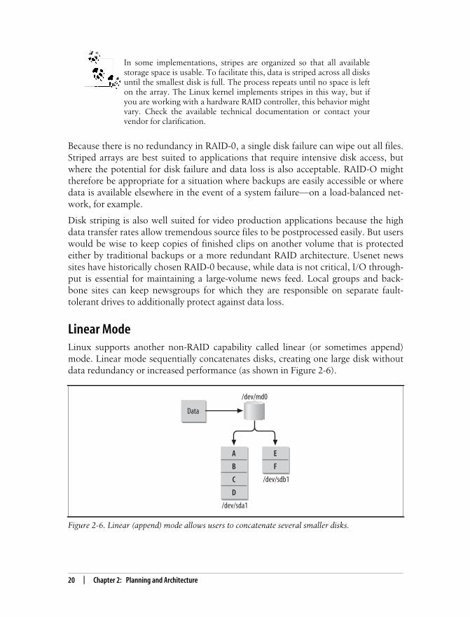
Linear ModeLinux supports another non-RAID capability called linear (or sometimes append)mode. Linear mode sequentially concatenates disks, creating one large disk withoutdata redundancy or increased performance (as shown in Figure 2-6).
Figure 2-6. Linear (append) mode allows users to concatenate several smaller disks.
/dev/md0
E
F
A
B
C
D
Data
/dev/sda1
/dev/sdb1

This is the Title of the Book, eMatter EditionCopyright © 2008 O’Reilly & Associates, Inc. All rights reserved.
The RAID Levels: In Depth | 21
Linear arrays are most useful when working with disks and controllers of varyingsizes, types, and speeds. Disks belonging to linear arrays are written to until they arefull. Since data is not interleaved across the member disks, parallel operations thatcould be affected by a single disk bottleneck do not occur, as they can in RAID-0. Nospace is ever wasted when working with linear arrays, regardless of differing disksizes. Over time, however, as data becomes more spread out over a linear array, youwill see performance differences when accessing files that are on different disks ofdiffering speeds and sizes, and when you access a file that spans more than one disk.
Like RAID-0, linear mode arrays offer no redundancy. A disk failure means com-plete data loss, although recovering data from a damaged array might be a bit easierthan with RAID-0, because data is not interleaved across all disks. Because it offersno redundancy or performance improvement, linear mode is best left for desktop andhobbyist use.
Linear mode, and to a lesser degree, RAID-0, are also ideal for recycling old drivesthat might not have practical application when used individually. A spare disk con-troller can easily turn a stack of 2- or 3-gigabyte drives into a receptacle for storingmovies and music to annoy the RIAA and MPAA.
RAID-1 (Mirroring)RAID-1 provides the most complete form of redundancy because it can survive mul-tiple disk failures without the need for special data recovery algorithms. Data is mir-rored block-by-block onto each member disk (see Figure 2-7). So for every N disks ina RAID-1, the array can withstand a failure of N-1 disks without data loss. In a four-disk RAID-1, up to three disks could be lost without loss of data.
As the number of member disks in a mirror increases, the write performance of thearray decreases. Each write incurs a performance hit because each block must be
Figure 2-7. Fully redundant RAID-1.
/dev/md0
A
B
C
D
A
B
C
D
Data
/dev/sda1 /dev/sdb1

This is the Title of the Book, eMatter EditionCopyright © 2008 O’Reilly & Associates, Inc. All rights reserved.
22 | Chapter 2: Planning and Architecture
written to each participating disk. However, a substantial advantage in read perfor-mance is achieved through parallel access. Duplicate copies of data on different harddrives allow the system to make concurrent read requests.
For example, let’s examine the read and write operations of a two-disk RAID-1. Let’ssay that I’m going to perform a database query to display a list of all the customersthat have ordered from my company this year. Fifty such customers exist, and eachof their customer data records is 1 KB. My RAID-1 array receives a request to retrievethese fifty customer records and output them to my company’s sales engineer. Thedrives in my array store data in 1 KB chunks and support a data throughput of 1 KBat a time. However, my controller card and system bus support a data throughput of2 KB at a time. Because my data exists on more than one disk drive, I can utilize thefull potential of my system bus and disk controller despite the limitation of my harddrives.
Suppose one of my sales engineers needs to change information about each of thesame fifty customers. Now we need to write fifty records, each consisting of 1 KB.Unfortunately, we need to write each chunk of information to both drives in ourarray. So in this case, we need to write 100 KB of data to our disks, rather than 50KB. The number of write operations increases with each disk added to a mirrorarray. In this case, if the array had four member disks, a total of 4 KB would be writ-ten to disk for each 1 KB of data passed to the array.
This example reveals an important distinction between hardware and softwareRAID-1. With software RAID, each write operation (one per disk) travels over thePCI bus to corresponding controllers and disks (see the sections “Motherboards andthe PCI Bus” and “I/O Channels,” later in this chapter). With hardware RAID, onlya single write operation travels over the PCI bus. The RAID controller sends theproper number of write operations out to each disk. Thus, with hardware RAID-1,the PCI bus is less saturated with I/O requests.
Although RAID-1 provides complete fault tolerance, it is cost-prohibitive for someusers because it at least doubles storage costs. However, for sites that require zerodowntime, but are willing to take a slight hit on write performance, mirroring isideal. Such sites might include online magazines and newspapers, which serve a largenumber of customers but have relatively static content. Online advertising aggrega-tors that facilitate the distribution of banner ads to customers would also benefitfrom disk mirroring. If your content is nearly static, you won’t suffer much from thewrite performance penalty, while you will benefit from the parallel read-as-you-serveimage files. Full fault tolerance ensures that the revenue stream is never interruptedand that users can always access data.
RAID-1 works extremely well when servers are already load-balanced at the networklevel. This means usage can be distributed across multiple machines, each of whichsupports full redundancy. Typically, RAID-1 is deployed using two-disk mirrors.Although you could create mirrors with more disks, allowing the system to survive a
This is the Title of the Book, eMatter EditionCopyright © 2008 O’Reilly & Associates, Inc. All rights reserved.
The RAID Levels: In Depth | 23
multiple disk failure, there are other arrangements that allow comparable redun-dancy and read performance and much better write performance. See the “HybridArrays” section, later in this chapter. RAID-1 is also well suited for system disks.
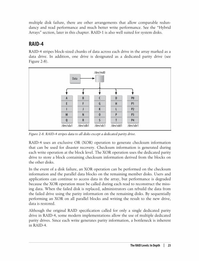
RAID-4RAID-4 stripes block-sized chunks of data across each drive in the array marked as adata drive. In addition, one drive is designated as a dedicated parity drive (seeFigure 2-8).
RAID-4 uses an exclusive OR (XOR) operation to generate checksum informationthat can be used for disaster recovery. Checksum information is generated duringeach write operation at the block level. The XOR operation uses the dedicated paritydrive to store a block containing checksum information derived from the blocks onthe other disks.
In the event of a disk failure, an XOR operation can be performed on the checksuminformation and the parallel data blocks on the remaining member disks. Users andapplications can continue to access data in the array, but performance is degradedbecause the XOR operation must be called during each read to reconstruct the miss-ing data. When the failed disk is replaced, administrators can rebuild the data fromthe failed drive using the parity information on the remaining disks. By sequentiallyperforming an XOR on all parallel blocks and writing the result to the new drive,data is restored.
Although the original RAID specification called for only a single dedicated paritydrive in RAID-4, some modern implementations allow the use of multiple dedicatedparity drives. Since each write generates parity information, a bottleneck is inherentin RAID-4.
Figure 2-8. RAID-4 stripes data to all disks except a dedicated parity drive.
/dev/md0
Data
C
G
K
O
S
/dev/sdc1
P0
P1
P2
P3
P4
/dev/sde1
B
F
J
N
R
/dev/sdb1
A
E
I
M
Q
/dev/sda1
D
H
L
P
T
/dev/sdd1

This is the Title of the Book, eMatter EditionCopyright © 2008 O’Reilly & Associates, Inc. All rights reserved.
24 | Chapter 2: Planning and Architecture
Placing the parity drive at the beginning of an I/O channel and giving it the lowestSCSI ID in that chain will help improve performance. Using a dedicated channel forthe parity drive is also recommended.
It is very unlikely that RAID-4 makes sense for any modern setup. With the excep-tion of some specialized, turnkey RAID hardware, RAID-4 is not often used. RAID-5provides better performance and is likely a better choice for anyone who is consider-ing RAID-4. It’s prudent to mention here, however, that many NAS vendors still useRAID-4 simply because online array expansion is easier to implement and expansionis faster than with RAID-5. That’s because you don’t need to reposition all the parityblocks when you expand a RAID-4.
Dedicating a drive for parity information means that you lose one drive’s worth ofpotential data storage when using RAID-4. When using N disk drives, each withspace S, and dedicating one drive for parity storage, you are left with (N-1) * S spaceunder RAID-4. When using more than one parity drive, you are left with (N-P) * Sspace, where P represents the total number of dedicated parity drives in the array.
RAID-5RAID-5 eliminates the use of a dedicated parity drive and stripes parity informationacross each disk in the array, using the same XOR algorithm found in RAID-4 (see
XORThe exclusive OR (XOR) is a logical operation that returns a TRUE value if and only ifone of the operands is TRUE. If both operands are TRUE, then a value of FALSE is returned.
p q p XOR q-----------------------T T FT F TF T TF F T
When a parity RAID generates its checksum information, it performs the XOR on eachdata byte. For example, a RAID-5 with three member disks writes the byte 11011011binary to the first disk and the byte 01101100 to the second disk. The first two bytesare user data. Next, a parity byte of 10110111 is written to the third disk. If a byte islost because of the failure of either the first or the second disk, the array can performthe XOR operation on the other data byte and the parity information in order toretrieve the missing data byte. This holds true for any number of data bytes or, in ourcase, disks.

This is the Title of the Book, eMatter EditionCopyright © 2008 O’Reilly & Associates, Inc. All rights reserved.
The RAID Levels: In Depth | 25
Figure 2-9). During each write operation, one chunk worth of data in each stripe isused to store parity. The disk that stores parity alternates with each stripe, until eachdisk has one chunk worth of parity information. The process then repeats, begin-ning with the first disk.
Take the example of a RAID-5 with five member disks. In this case, every fifthchunk-sized block on each member disk will contain parity information for the otherfour disks. This means that, as in RAID-1 and RAID-4, a portion of your total stor-age space will be unusable. In an array with five disks, a single disk’s worth of spaceis occupied by parity information, although the parity information is spread acrossevery disk in the array. In general, if you have N disk drives in a RAID-5, each of sizeS, you will be left with (N-1) * S space available. So, RAID-4 and RAID-5 yield thesame usable storage. Unfortunately, also like RAID-4, a RAID-5 can withstand only asingle disk failure. If more than one drive fails, all data on the array is lost.
RAID-5 performs almost as well as a striped array for reads. Write performance onfull stripe operations is also comparable, but when writes smaller than a single stripeoccur, performance can be much slower. The slow performance results from preread-ing that must be performed so that corrected parity can be written for the stripe.During a disk failure, RAID-5 read performance slows down because each time datafrom the failed drive is needed, the parity algorithm must reconstruct the lost data.Writes during a disk failure do not take a performance hit and will actually beslightly faster. Once a failed disk is replaced, data reconstruction begins either auto-matically or after a system administrator intervenes, depending on the hardware.
RAID-5 has become extremely popular among Internet and e-commerce companiesbecause it allows administrators to achieve a safe level of fault-tolerance without sac-rificing the tremendous amount of disk space necessary in a RAID-1 configuration orsuffering the bottleneck inherent in RAID-4. RAID-5 is especially useful in produc-tion environments where data is replicated across multiple servers, shifting the inter-nal need for disk redundancy partially away from a single machine.
Figure 2-9. RAID-5 eliminates the dedicated parity disk by distributing parity across all drives.
/dev/md0
Data
C
G
P2
N
R
/dev/sdc1
P0
H
L
P
T
/dev/sde1
B
F
J
P3
Q
/dev/sdb1
A
E
I
M
P4
/dev/sda1
D
P1
K
O
S
/dev/sdd1

This is the Title of the Book, eMatter EditionCopyright © 2008 O’Reilly & Associates, Inc. All rights reserved.
26 | Chapter 2: Planning and Architecture
Hybrid ArraysAfter the Berkeley Papers were published, many vendors began combining differentRAID levels in an attempt to increase both performance and reliability. These hybridarrays are supported by most hardware RAID controllers and external systems. TheLinux kernel will also allow the combination of two or more RAID levels to form ahybrid array. In fact, it allows any combination of arrays, although some of themmight not offer any benefit. The most common types of hybrid arrays, summarizedin the following sections, are covered in this book.
RAID-10 (striping mirror)
The most widely used, and effective, hybrid array results from the combination ofRAID-0 and RAID-1. The fast performance of striping, coupled with the redundantproperties of mirroring, create a quick and reliable solution—although it is the mostexpensive solution.
A striped-mirror, or RAID-10, is simple. Two separate mirrors are created, each witha unique set of member disks. Then the two mirror arrays are added to a new stripedarray (see Figure 2-10). When data is written to the logical RAID device, it is stripedacross the two mirrors.
Figure 2-10. A hybrid array formed by combining two mirrors, which are then combined into astripe.
/dev/md0(RAID 0)
Data
/dev/md1
A
C
E
G
A
C
E
G
/dev/md2
B
D
F
H
B
D
F
H
RAID 1 RAID 1

This is the Title of the Book, eMatter EditionCopyright © 2008 O’Reilly & Associates, Inc. All rights reserved.
The RAID Levels: In Depth | 27
Although this arrangement requires a lot of surplus disk hardware, it provides a fastand reliable solution. I/O approaches a throughput close to that of a standalonestriped array. When any single disk in a RAID-10 fails, both sides of the hybrid (eachmirror) may still operate, although the one with the failed disk will be operating indegraded mode. A RAID-10 arrangement could even withstand multiple disk fail-ures on different sides of the stripe.
When creating a RAID-10, it’s a good idea to distribute the mirroring arrays acrossmultiple I/O channels. This will help the array withstand controller failures. Forexample, take the case of a RAID-10 consisting of two mirror sets, each containingtwo member disks. If each mirror is placed on its own I/O channel, then a failure ofthat channel will render the entire hybrid array useless. However, if each memberdisk of a single mirror is placed on a separate channel, then the array can withstandthe failure of an entire I/O channel (see Figure 2-11).
While you could combine two stripes into a mirror, this arrangement offers noincrease in performance over RAID-10 and does not increase redundancy. In fact,RAID-10 can withstand more disk failures than what many manufacturers call RAID-0+1 (two stripes combined into a mirror). While it’s true that a RAID-0+1 could sur-vive two disk failures within the same stripe, that second disk failure is trivialbecause it’s already part of a nonfunctioning stripe.
I’ve mentioned earlier that vendors often deviate from naming conventions whendescribing RAID. This is especially true with hybrid arrays. Make sure that your con-troller combines mirrors into a stripe (RAID-10) and not stripes into a mirror (RAID-0+1).
Figure 2-11. Spreading the mirrors across multiple I/O channels increases redundancy.
Disk controllerB
Disk controllerA
Mirror 1Disk 1
Mirror 2Disk 1
Mirror 1Disk 2
Mirror 2Disk 2
One disk from each side could also fail.
RAID 0

This is the Title of the Book, eMatter EditionCopyright © 2008 O’Reilly & Associates, Inc. All rights reserved.
28 | Chapter 2: Planning and Architecture
RAID-50 (striping parity)
Users who simply cannot afford to build a RAID-0+1 array because of the enormousdisk overhead can combine two RAID-5 arrays into a striped array (see Figure 2-12).While read performance is slightly lower than a RAID-0+1, users will see increasedwrite performance because each side of the stripe is made up of RAID-5 arrays,which also utilize disk striping. Each side of the RAID-50 array can survive a singledisk failure. A failure of more than one disk in either RAID-5, though, would resultin failure of the entire RAID-50.
RAID Case Studies: What Should I Choose?Choosing an architecture can be extremely difficult. Trying to connect a specifictechnology to a specific application is one of the hardest tasks that system adminis-trators face. Below are some examples of where RAID is useful in the real world.
Case 1: HTTP Image ServerBecause RAID-1 supports parallel reads, it makes a great HTTP image server. Com-panies that sell products online and provide product photos to web surfers could useRAID-1 to serve images. Images are static content, and in this scenario, they willlikely be read quite a bit more than they will be written. Although new product pho-tos are frequently added, they are written to disk only once by a web developer,whereas they are viewed thousands of times by potential customers. Parallel readperformance on RAID-1 helps facilitate the large number of hits, and the write per-formance loss with RAID-1 is largely irrelevant because writes are infrequent in this
Figure 2-12. A hybrid array formed by combining RAID-5 arrays into a striped array.
/dev/md0(RAID 0)
/dev/md1
E
M
P2
AA
II
P0
O
W
EE
MM
C
K
S
P3
GG
A
I
Q
Y
P4
G
P1
U
CC
KK
/dev/md2
F
N
P2
BB
JJ
P0
P
X
FF
D
L
T
P3
HH
B
J
R
Z
P4
H
P1
V
DD
LL
Data
RAID 5RAID 5
NN

This is the Title of the Book, eMatter EditionCopyright © 2008 O’Reilly & Associates, Inc. All rights reserved.
RAID Case Studies: What Should I Choose? | 29
case. The redundancy aspect of RAID-1 also ensures that downtime is minimal in theevent of a disk failure, although parallel read performance will be temporarily lostuntil the drive can be replaced. Using a hot-spare, of course, ensures that perfor-mance is affected for only a brief time.
Case 2: Usenet NewsStriped arrays are clearly the best candidate for Internet news servers. Extremely fastread and write times are required to keep up with the enormous streams of data thata typical full-feed news server experiences. In many cases, the data on a news parti-tion is inconsequential. Lost articles are frequent, even in normally operating feeds,and complete data loss usually means that only a few days’ articles are lost.
Administrators could configure a single news server with both a striped array andmirrored array, as shown in Figure 2-13. The striped array could house newsgroupsthat are of no consequence and could easily withstand a day’s worth of article losswithout users complaining. Newsgroups that are read frequently, as well as localgroups and system partitions, could be housed on the RAID-1 array. This wouldmake the machine redundant in case of a disk failure.
Case 3: Home Use (Digital Audio, Video, and Images)With the increasing capacity and availability of digital media, users will find it diffi-cult to contain their files on a single hard disk. Linear mode and RAID-0 arrays pro-vide a good storage architecture for storing MP3 audio, video, and image files. Often,these files are burned to CD or are easily replaceable, so the lack of redundancy in
Figure 2-13. A Usenet news server with both a striped and mirror array.
//home/usr/var/swap/var/spool/news/local
/dev/sda
//home/usr/var/swap/var/spool/news/local
/dev/sdb
RAID 1: System drives and local groups
RAID 0: Internet news groups
/var/spool/news/
Data-AData-CData-E. . .
/dev/sdc /dev/sdd
/var/spool/news/
Data-BData-DData-F. . .

This is the Title of the Book, eMatter EditionCopyright © 2008 O’Reilly & Associates, Inc. All rights reserved.
30 | Chapter 2: Planning and Architecture
linear mode and RAID-0 can be overlooked. Users can opt to make backups of filesthat are either important or hard to replace.
A quick trip to a surplus warehouse or .COM auction might get you a supply ofolder, cheap hard disks that can be combined into a linear array. If you can findmatched disks, then RAID-0 will work well in this case. A mix of different drives canbe turned into a linear mode array. Both of these methods are perfect for home usebecause they maximize what might have become old and useless storage space andturn it into usable disk space.
Case 4: The Acme Motion Picture CompanyPeople who produce motion pictures are faced with many storage problems. Accom-modating giant source files, providing instant access to unedited footage, and stor-ing a finished product that could easily exceed hundreds of gigabytes are just a few ofthe major storage issues that the film and television industries face.
Film production workstations would benefit greatly from RAID-5. While RAID-0might seem like a good choice because of its fast performance, losing a work-in-progress might set work back by days, or even weeks. By using RAID-5, editors areable to achieve redundancy and see an improvement in performance. Likewise,RAID-1 might seem like a good choice because it offers redundancy without much ofa performance hit during disk failures. But RAID-1, as discussed earlier, leads to anincrease only in read performance, and editors will likely be writing postproducedclips often until the desired cut is achieved.
Source files and finished scenes would benefit most from RAID-1 setups. Worksta-tions could read source files from these RAID-1 servers. Parallel reads would alloweditors and production assistants to quickly pull in source video that could then beedited locally on the RAID-5 array, where write performance is better than on RAID-1. When a particular scene is completed, it could then be sent back to the RAID-1array for safekeeping. Although write performance on RAID-1 isn’t as fast as onRAID-5, the redundancy of RAID-1 is essential for ensuring that no data is ever lost.Reshooting a scene could be extremely costly and, in some cases, impossible.
Figure 2-14 shows how different RAID arrays could be used in film production.
Striping might also be a good candidate for film production workstations. If cost is aconsideration, using RAID-0 will save slightly on drive costs and will outperformRAID-5. But a drive failure in a RAID-0 workstation would mean complete data loss.
Case 5: Video on DemandThis scenario offers the same considerations as Case 1, the site serving images.RAID-1, with multiple member disks, offers great read performance. Since writesaren’t very frequent when working with video on demand, the write performance hitis okay.

This is the Title of the Book, eMatter EditionCopyright © 2008 O’Reilly & Associates, Inc. All rights reserved.
Disk Failures | 31
Disk FailuresAnother benefit of RAID is its ability to handle disk failures without user interven-tion. Redundant arrays can not only remain running during a disk failure, but canalso repair themselves if sufficient replacement hardware is available and was precon-figured when the array was created.
Degraded ModeWhen an array member fails for any reason, the array is said to have gone intodegraded mode. This means that the array is not performing optimally and redun-dancy has been compromised. Degraded mode therefore applies only to arrays thathave redundant capabilities. A RAID-0, for example, has only two states: opera-tional and failed. This interim state, available to redundant arrays, allows the array tocontinue operating until an administrator can resolve the problem—usually byreplacing a failed disk.
Hot-SparesAs I mentioned earlier, some RAID levels can replace a failed drive with a new drivewithout user intervention. This functionality, known as hot-spares, is built into everyhardware RAID controller and standalone array. It is also part of the Linux kernel. Ifyou have hardware that supports hot-spares, then you can identify some extra disksto act as spares when a drive failure occurs. Once an array experiences a disk failure,and consequently enters into degraded mode, a hot-spare can automatically be intro-duced into the array. This makes the job of the administrator much easier, becausethe array immediately resumes normal operation, allowing the administrator toreplace failed drives when convenient. In addition, having hot-spares decreases thechance that a second drive will fail and cause data loss.
Figure 2-14. Workstations with RAID-5 arrays edit films while retrieving source films from aRAID-1 array. Finished products are sent to another RAID-1 array.
RAID 1Source media Backup
server
RAID 1Finished projects
Video production workstations(RAID 5)

This is the Title of the Book, eMatter EditionCopyright © 2008 O’Reilly & Associates, Inc. All rights reserved.
32 | Chapter 2: Planning and Architecture
Hot-spares can be used only with arrays that support redundancy:mirrors, RAID-4, and RAID-5. Striped and linear mode arrays do notsupport this feature.
Hot-SwapAll of the RAID levels that support redundancy are also capable of hot-swap. Hot-swap is the ability to removed a failed drive from a running system so that it can bereplaced with a new working drive. This means drive replacement can occur withouta reboot. Hot-swap is useful in two situations. First, you might not have enoughspace in your cases to support extra disks for the hot-spare feature. So when a diskfailure occurs, you may want to immediately replace the failed drive in order to bringthe array out of degraded mode and begin reconstruction. Second, although youmight have hot-spares in a system, it is useful to replace the failed disk with a newhot-spare in anticipation of future failures.
Replacing a drive in a running system should not be attempted on a conventionalsystem. While hot-swap is inherently supported by RAID, you need special hard-ware that supports it. This technology was originally available only to SCSI usersthrough specially made hard drives and cases. However, some companies now makehot-swap ATA enclosures, as well as modules that allow you to safely hot-swap nor-mal SCSI drives. For more information about hot-swap, see the “Cases, Cables, andConnectors” section, later in this chapter, and the “Managing Disk Failures” sectionin Chapter 7.
Although many people have successfully disconnected traditionaldrives from running systems, it is not a recommended practice. Do thisat your own risk. You could wipe your array or electrocute yourself.
Hardware ConsiderationsWhether you choose to use kernel-based software RAID or buy a specialized RAIDcontroller, there are some important decisions to make when buying components.Even if you plan to use software RAID, you will still need to purchase hard drivesand disk controllers. The first step is to determine the ultimate size of your array andfigure out how many drives are necessary to accommodate all the space you need,taking into account the extra space required by the level of RAID you choose. Don’tforget to factor the eventual need for hot-spares into your plan.
Choosing the right components can be the hardest decision to make when building aRAID system. If you’re building a production server, you should naturally buy thebest hardware you can afford. If you’re just experimenting, then use whatever youhave at your disposal, but realize that you may have to shell out a few dollars tomake things work properly.

This is the Title of the Book, eMatter EditionCopyright © 2008 O’Reilly & Associates, Inc. All rights reserved.
Hardware Considerations | 33
Several factors will ultimately affect the performance and expandability of yourarrays:
• Bus throughput
• I/O channels
• Disk protocol throughput
• Drive speed
• CPU speed and memory
Computer architecture is a vast and complicated topic, and although this book cov-ers the factors that will most drastically impact array performance, I advise anyonewho is planning to build large-scale production systems, or build RAID systems forresale, to familiarize themselves thoroughly with all of the issues at hand. A com-plete primer on computer architecture is well beyond the scope of this book. The“Bibliography” section of the Appendix contains a list of excellent books and websites for readers who wish to expand their knowledge of computer hardware.
One essential concept that I do want to introduce is the bottleneck. Imagine the fil-tered water pitchers that have become so omnipresent over the last ten years. Whenyou fill the chamber at the top of the pitcher with ordinary tap water, it slowly dripsthrough the filter into another cache, from which you can pour a glass of water. Thefiltering process distributes water at a rate much slower than the pressure of an ordi-nary faucet. The filter has therefore introduced a bottleneck in your ability to fillyour water glass, although it does provide some benefits. A more expensive filtrationsystem might be able to yield better output and cleaner water. A cheaper systemcould offer quicker filtration with some sacrifices in quality, or better quality at aslower pace.
In computing, a bottleneck occurs when the inadequacies of a single componentcause a slowdown of the entire system. The slowdown might be the result of poorsystem design, overuse, or both. Each component of your system has the potential tobecome a bottleneck if it’s not chosen carefully. As you will learn throughout thischapter, some bottlenecks are simply beyond your control, while others begin tooffer diminishing returns as you upgrade them.
An Organizational OverviewAll systems are built around a motherboard. The motherboard integrates all the com-ponents of a computer by providing a means through which processors, memory,peripherals, and user devices (monitors, keyboards, and mice) can communicate.Specialized system controllers facilitate communication between these devices. Thisgroup of controllers is often referred to as the motherboard’s chipset. In addition tofacilitating communication, the chipset also determines factors that affect systemexpandability, such as maximum memory capacity and processor speed.

This is the Title of the Book, eMatter EditionCopyright © 2008 O’Reilly & Associates, Inc. All rights reserved.
34 | Chapter 2: Planning and Architecture
When an application needs data, the CPU first checks to see if the data is stored inmemory. If the data is no longer in memory, the CPU asks the chipset to request theinformation from disk. The chipset sends a request to the data bus, where it is pickedup by the appropriate disk controller and sent across the disk bus to the drive con-taining the data. The drive sends the information back to the controller card, whichin turn passes it back to the CPU and main memory. Figure 2-15 illustrates the con-nections between various components of a modern PCI motherboard.
The speeds of the data and disk buses have a direct impact on system performance,and each bus can become a bottleneck. While it’s easy to add new disk controllers toa system, thereby increasing the overall number of disk buses, and consequentlyincreasing the overall disk bus throughput, you only have one motherboard to workwith. So choosing the right one for your application is essential.
Figure 2-15. When disk I/O occurs, data travels over both the data bus and the disk bus, each apotential bottleneck.
The BIOSAnother important component of every computer system is the BIOS (basic input/out-put software). The BIOS is a chip on the motherboard that contains a simple set of driv-ers and instructions. When a machine is turned on, the software stored in the BIOSchip is loaded and executed. The BIOS has basic control over system components:hard disks, CD-ROMs, monitors, keyboards, etc. The BIOS looks for a particular disksector and executes the program it finds there, usually an operating system. This issometimes referred to as the bootstrap process.
Diskcontroller
Graphicsadaptor
Diskcontroller
Disk bus Disk bus
Networkadaptor
Data bus
Memory bus
Systemcontrolchipset
Memory
CPU
Parallel,serial,
and ATAconnections

This is the Title of the Book, eMatter EditionCopyright © 2008 O’Reilly & Associates, Inc. All rights reserved.
Hardware Considerations | 35
Motherboards and the PCI BusMotherboards provide a way to interconnect the various components that make up acomputer (memory, processors, and peripherals). Every motherboard has separatebuses for communicating between these varied components. Disk controllers and, inturn, hard disks, communicate with the CPU and memory using the I/O bus, alsocalled the data bus. The I/O bus is a standard interface through which peripheralcards (disk controllers, graphics adapters, network cards, etc.) can interface betweenperipherals (hard disks, monitors, Ethernet networks, etc.) and the CPU and mem-ory.
The Peripheral Component Interconnect (PCI) bus is the most common data busavailable today. In recent years, it has usurped the ubiquity of the now outdatedIndustry Standard Architecture (ISA) bus. Although ISA motherboards are still com-mon, new motherboard purchases typically use the PCI bus. For backward compati-bility, the PCI bus can handle ISA peripheral cards through the use of bridging, andmany PCI motherboards provide an ISA slot for use with legacy cards.
Bus-width and bus-speed
The speed of the I/O bus is determined by two factors: bus-width and bus-speed. Bus-width describes how many bytes of data can be sent down the bus at a time. Bus-speed specifies how many times per second data can be transferred through the bus.Bus-width is measured in bits, and all motherboards support bus-widths in multi-ples of bytes. ISA motherboards support bus-widths of 8 and 16 bits (1 or 2 bytes),and modern PCI motherboards support bus-widths of up to 64 bits, or 8 bytes.
Bus-speed is measured by the number of clock cycles that can occur each second.Manufacturers now use the term Front Side Bus when referring to bus-speed. ISAboards run at 8.33 MHz, or 8.33 million clock cycles per second. The first PCIboards ran at 33.33 MHz, or 33.33 million clock cycles per second. A PCI mother-board with a 32-bit bus-width (4 bytes), operating at 33 MHz, has a maximum I/Othroughput of 133.33 MB/s (4 bytes per cycle * 33.33 million cycles per second =133.33 megabytes per second). Newer and faster PCI boards can operate at speeds ofup to 533 MHz. Table 2-3 shows the various I/O throughputs of typical mother-boards as a factor of bus-width and bus-speed.
Table 2-3. I/O bus throughput
Bus type Width (bits) Clock cycles (MHz) Data throughput (MB/s)
ISA (XT) 8 8.33 8.33
ISA (AT) 16 8.33 16.66
PCI 32 33.33 133.33
PCI 64 66.66 533.33

This is the Title of the Book, eMatter EditionCopyright © 2008 O’Reilly & Associates, Inc. All rights reserved.
36 | Chapter 2: Planning and Architecture
The data throughput of your motherboard is the first bottleneck to consider whenbuilding a RAID system. If you are planning to use three SCSI cards, each with anadvertised speed of 80 MB/s, you should quickly realize that a standard 32-bit PCImotherboard running at 33 MHz will become a bottleneck. The aggregate speed ofyour SCSI controllers (80 MB/s * 3 = 240 MB/s) is more than the overall speed ofyour I/O bus (133.33 MB/s).
Not all motherboards are created equal. Be certain to check the manufacturer’s spec-ification when deciding which one to purchase, making careful note of the bus-widthand bus-speed. Remember that all the expansion cards, including the graphics card,share the overall speed of the I/O bus. If you have a board that supports an overallbus throughput of 533 MB/s, then installing several high-end SCSI cards, a graphicsadapter, and a network card might cause a bottleneck on the data bus. So for pro-duction file servers, it might make sense to configure a system without video (youcould use the console on serial port features of Linux). Like most other aspects oftechnology, you should expect to see faster motherboards in the near future.Although 128-bit boards might be a year or two off, manufacturers are constantlyworking to increase the bus-speed.
In the same way that disks constantly fall behind the curve of storage needs, the I/Obus is always behind the curve when compared to the speed at which the CPU andmain memory can interact. So the I/O bus will almost always become the most sig-nificant bottleneck on any motherboard. In response to this problem, it is commonfor high-end server boards to offer dedicated buses for one or more PCI slots. Someeven offer a separate bus for each PCI slot, which allows you to place a RAID or SCSIcard on its own I/O bus, separating other peripherals such as network and graphicscards. Using one of these dual-bus motherboards can effectively double the com-bined overall speed of your I/O bus.
I/O ChannelsAn I/O channel represents a single chain of devices attached to your machine, eitherinternally or externally. Internal I/O channels are typically connected to a controllercard (or to the motherboard) by ribbon cable. (Ribbon cables are flat cables, usually
64-Bit MotherboardsWhile some motherboards are advertised as having 64-bit PCI slots, usually only oneor two of the PCI slots are usable by 64-bit PCI cards. Fortunately, many 64-bit cardscan fit into 32-bit slots and operate in 32-bit mode. However, using 64-bit cards in 32-bit mode wastes their capability—they can operate at only half of their potential speed.So when choosing a 64-bit motherboard, be certain that it has enough 64-bit slots tomeet your needs.

This is the Title of the Book, eMatter EditionCopyright © 2008 O’Reilly & Associates, Inc. All rights reserved.
Hardware Considerations | 37
gray or blue, that interconnect hard drives and disk controllers inside a computercase.) Externally, you might connect drives or peripheral devices to a controller cardusing SCSI cables. The more identical, parallel I/O channels you have available foryour array, the better performance you can expect out of it, as long as you are care-ful to identify and eliminate other bottlenecks.
The most common instance of parallel and identical I/O channels is the typical PCmotherboard. Almost all i386-based motherboards include two onboard ATA/IDEdisk controllers (see Figure 2-16).
When I say identical, I mean that each channel you select for use in your array sup-ports the same architecture and protocols. Parallel means that each channel in thearray can accept requests simultaneously. While you could theoretically use two dif-ferent types of I/O channels in the same RAID array, you’d be wasting the perfor-mance of the faster channel because the faster chain needs to operate at slower ratein order to stay at the same pace as the other channels in the array. It’s generally nota good idea to mix different iterations of the same disk protocol because their speedsvary.
It’s also a bad idea to mix different disk protocols, such as SCSI and ATA, eventhough software RAID, in particular, allows both of these arrangements. The same istrue for mixing hard drives of differing speeds, but I’ll cover that issue in more detailin the “Choosing Hard Drives” section, later in this chapter.
In general, it is good practice to keep only one incarnation of any disk protocol on asingle I/O channel. That might mean connecting devices such as CD-ROM drivesand scanners, which operate at much slower speeds than current hard disks, on sepa-rate controllers. It is advisable to purchase a cheaper, slower controller to connectthese devices, keeping them out of any I/O channel that contains faster devices thatbelong to an array.
For example, many SCSI controllers contain two separate, parallel channels that arenot identical: a compact, high-density, 68-pin connector used to connect hard drives(wide SCSI) and a larger, low-density 50-pin connector often intended to connect
Figure 2-16. Major components on a motherboard.
CPUAGP/PCI slots
Primary/secondaryATA ports
Memory
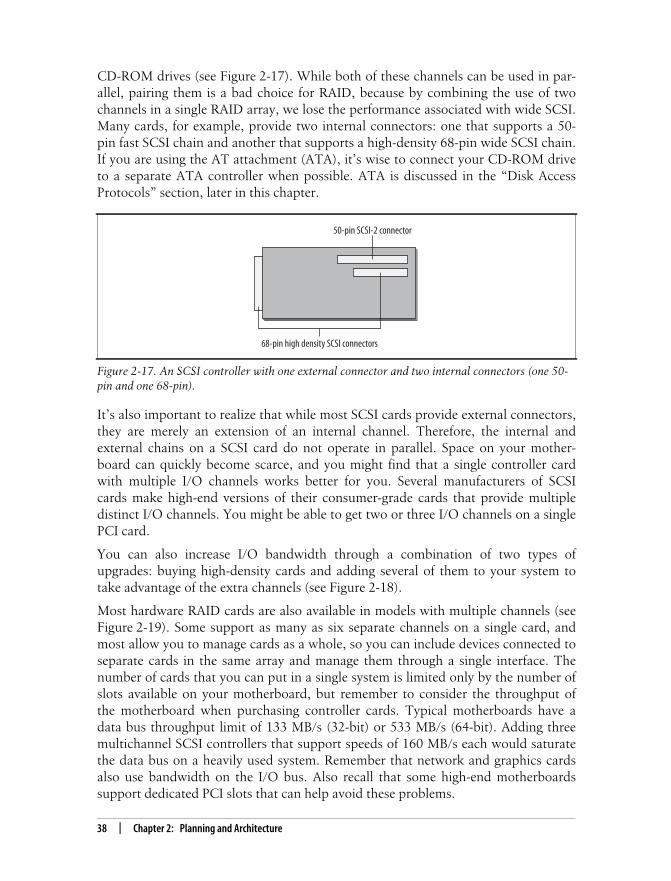
This is the Title of the Book, eMatter EditionCopyright © 2008 O’Reilly & Associates, Inc. All rights reserved.
38 | Chapter 2: Planning and Architecture
CD-ROM drives (see Figure 2-17). While both of these channels can be used in par-allel, pairing them is a bad choice for RAID, because by combining the use of twochannels in a single RAID array, we lose the performance associated with wide SCSI.Many cards, for example, provide two internal connectors: one that supports a 50-pin fast SCSI chain and another that supports a high-density 68-pin wide SCSI chain.If you are using the AT attachment (ATA), it’s wise to connect your CD-ROM driveto a separate ATA controller when possible. ATA is discussed in the “Disk AccessProtocols” section, later in this chapter.
It’s also important to realize that while most SCSI cards provide external connectors,they are merely an extension of an internal channel. Therefore, the internal andexternal chains on a SCSI card do not operate in parallel. Space on your mother-board can quickly become scarce, and you might find that a single controller cardwith multiple I/O channels works better for you. Several manufacturers of SCSIcards make high-end versions of their consumer-grade cards that provide multipledistinct I/O channels. You might be able to get two or three I/O channels on a singlePCI card.
You can also increase I/O bandwidth through a combination of two types ofupgrades: buying high-density cards and adding several of them to your system totake advantage of the extra channels (see Figure 2-18).
Most hardware RAID cards are also available in models with multiple channels (seeFigure 2-19). Some support as many as six separate channels on a single card, andmost allow you to manage cards as a whole, so you can include devices connected toseparate cards in the same array and manage them through a single interface. Thenumber of cards that you can put in a single system is limited only by the number ofslots available on your motherboard, but remember to consider the throughput ofthe motherboard when purchasing controller cards. Typical motherboards have adata bus throughput limit of 133 MB/s (32-bit) or 533 MB/s (64-bit). Adding threemultichannel SCSI controllers that support speeds of 160 MB/s each would saturatethe data bus on a heavily used system. Remember that network and graphics cardsalso use bandwidth on the I/O bus. Also recall that some high-end motherboardssupport dedicated PCI slots that can help avoid these problems.
Figure 2-17. An SCSI controller with one external connector and two internal connectors (one 50-pin and one 68-pin).
68-pin high density SCSI connectors
50-pin SCSI-2 connector

This is the Title of the Book, eMatter EditionCopyright © 2008 O’Reilly & Associates, Inc. All rights reserved.
Hardware Considerations | 39
When using more than one I/O channel, it’s advisable to alternate between channelswhen adding disks to an array. That will help you to avoid overloading a single I/O
Figure 2-18. Using multiple disk controllers increases both throughput and the total number ofusable drives.
Figure 2-19. Some controllers have multiple channels on a single card.
/dev/md0(RAID 0)
Data
Data bus
Disk controllerA
Disk controllerB
C
G
K
O
A
E
I
M
D
H
L
P
B
F
J
N
/dev/sda1 /dev/sdc1 /dev/sdb1 /dev/sdd1
/dev/md0(RAID 0)
Data
Data bus
Disk controllerchannel A
Disk controllerchannel B
C
G
K
O
A
E
I
M
D
H
L
P
B
F
J
N
/dev/sda1 /dev/sdc1 /dev/sdb1 /dev/sdd1

This is the Title of the Book, eMatter EditionCopyright © 2008 O’Reilly & Associates, Inc. All rights reserved.
40 | Chapter 2: Planning and Architecture
channel. You typically don’t need to worry about how you physically arrange yourdisks or how your hardware (or Linux) detects them. Just make certain that you bal-ance them as equally as possible between each available channel. When you createthe array, disks can be added in an arbitrary order so that their physical location canbe taken into account. This process might be facilitated through a configuration file,command-line utility, GUI management package, or BIOS utility. I’ll cover this pro-cess in more detail when I explain how to create new arrays in Chapters 3 and 4 (forsoftware RAID) and in Chapter 5 (for hardware RAID).
There may also be some situations when it is necessary to use drives with slightly dif-ferent performance. Let’s say, for example, that you have a few ultra-wide SCSIdrives from an assortment of different manufacturers. Since not all drives, regardlessof protocol, are exactly the same, you will see slightly different speeds from each. Inthis case, it’s best to arrange the drives so that the slowest has the smallest SCSI IDnumber and is closest to the controller. Likewise, the fastest should be placed far-thest from the controller and should be set to the highest SCSI ID number. This willhelp to alleviate the performance differences. Users who are planning to create a lin-ear mode array using several different drive sizes should arrange drives with thismethodology in mind. This methodology may also be helpful for users who simplycannot afford to purchase new, matched drives.
Disk Access ProtocolsThe disk protocol of the hardware you choose has a tremendous impact on the per-formance and scalability of your array. Each protocol has its own hard limits on themaximum throughput of each I/O channel and the maximum number of devices youcan attach to a single channel. So the disk protocol you select will have a directimpact on the maximum size of your array.
Although we traditionally think of RAID in terms of high-end SCSI systems, todayit’s not uncommon for consumer-marketed systems to come equipped with supportfor RAID on non-SCSI disks. In fact, Linux software RAID can support either SCSIor ATA devices as part of an array (see the following section). The kernel will even letyou mix these protocols within a single RAID device, although that arrangementisn’t recommended. (See the “Matched drives” section, later in this chapter, as wellas the previous section, “I/O Channels.”) Software RAID under Linux does not relyon the underlying disk architecture to work, so there is no reason why an array couldnot be built using a Firewire (IEEE 1394), Fiber-channel, or other disk architecturedeveloped in the future, as long as you can find hardware and device drivers to sup-port the architecture as a standalone device.
ATA (used interchangeably with the acronym IDE) and SCSI are discussed in detailthroughout this book because they are the most common disk protocols in usetoday. ATA is a part of every modern motherboard, and SCSI is the most commonchoice for large servers.

This is the Title of the Book, eMatter EditionCopyright © 2008 O’Reilly & Associates, Inc. All rights reserved.
Hardware Considerations | 41
The AT Attachment (ATA) and Integrated DiskElectronics (IDE)Integrated disk electronics, or IDE, has had many incarnations and many names sinceits introduction in 1986. Originally, hard drives were small enough, in both size andcapacity, to fit directly onto disk controllers. As storage requirements grew, manufac-turers realized that housing drives on controller cards was an inefficient use of space.Soon drives and controllers became separate entities, connected by ribbon cable.This meant that drives could grow in size without interfering with the expandabilityof the motherboard. It was common for these integrated controller cards to makeadjacent slots on the motherboard inaccessible. Manufacturers eventually decidedthat portions of the controller could be housed directly on the drives and that creat-ing a standard drive interface would allow for both expandability and portability.Originally called IDE in several proprietary implementations, a standardized versioncalled the AT Attachment, or ATA, was eventually ratified (although many peoplestill use the terms IDE and ATA interchangeably). This new disk interface was calledthe AT Attachment because it was introduced with the ISA (AT) motherboard. Itquickly grew in popularity, and today the ATA interface is the most widely deployedconsumer disk interface. Figure 2-20 shows the ATA interface.
ATA has evolved a great deal since its introduction. Its performance and scalabilityhave improved over time. Table 2-4 outlines the various iterations of ATA.
Figure 2-20. The ATA interface separated the drive and the controller.
Table 2-4. Overview of IDE/ATA types
ATA type Maximum throughput (MB/s) Common names
ATA-1 8.3 ATA, IDE, Fast ATA
ATA-2 16.66 EIDE, Fast ATA-2
ATA-3 16.66 Ultra DMA, Ultra ATA
ATA-4 33.33 Ultra ATA/33
ATA-5 66.66 Ultra ATA/66
ATA-6 100 Ultra ATA/100
ATA-7 133.33 Ultra ATA/133
ATA hard disk
Power40-pin connector
ATA connector
Motherboard
ATA ribboncable

This is the Title of the Book, eMatter EditionCopyright © 2008 O’Reilly & Associates, Inc. All rights reserved.
42 | Chapter 2: Planning and Architecture
Many of the names associated with various iterations of ATA represent departuresfrom the ATA specification by a single manufacturer. Enhanced IDE (EIDE), forexample, was an attempt by Western Digital to increase its market share by offeringenhancements to the original ATA (ATA-1) specification before ATA-2 was ratified.This created a rash of vendor-enhanced ATA-compatible interfaces, resulting inmany puzzling names. In general, ATA devices are compatible between iterations,but mixing old and new drives, like mixing different disk protocols, usually results inperformance problems.
Master and slave
ATA devices have only two configuration settings: master and slave. Despite theunfortunate nomenclature, both drives can operate independently once the systeminitializes, although drives operating in slave mode won’t perform as well. A singleATA disk operating as master on a dedicated channel will yield the best perfor-mance. So it’s always recommended that you use only one disk per channel whenworking with ATA and RAID.
Only the master device can be used as a boot device, but you can use the masterdevice from any ATA channel for booting. So on a standard system with two on-board ATA controllers, you have a maximum of two boot devices and a total of fourATA devices. Most users place their primary hard disk on the first interface and aCD-ROM drive on the second, so that either can be used as a boot device.
A simple jumper on the back of the drive determines whether an ATA device is oper-ating in master or slave mode. Some devices also have a third setting called cableselect. This jumper allows the system to determine which device is master or slave byits position on the cable. The first ATA device found on the cable is flagged as themaster device and the second becomes the slave device. Unfortunately, many usersreport strange behavior when using this feature, such as disappearing drives ordevices that won’t boot properly. Because it’s easy to manually set the devices, I rec-ommend always setting up devices as master and slave and never using cable select.
Direct memory access (DMA)
Modern ATA devices support an I/O method called direct memory access (DMA) thatallows two devices on the same channel to transfer data without direct CPU interven-tion. Using DMA relieves a lot of pressure on your CPU during array reconstruction,when large amounts of data need to be transferred between two drives. SometimesDMA is not enabled by default. Chapter 7 discusses how to enable this feature andfine-tune ATA disks.
The drawbacks of ATA
By far the biggest drawback of ATA is its real limit of two devices per channel and itsusable limit of one device per channel when performance is an issue. This limit hin-ders the scalability of any RAID built with ATA, in terms of performance and maximum

This is the Title of the Book, eMatter EditionCopyright © 2008 O’Reilly & Associates, Inc. All rights reserved.
Hardware Considerations | 43
storage. In fact, this limitation might be the determining factor in choosing SCSI overATA. While most motherboards come with two onboard ATA controllers, the four-disk maximum (which really translates into two RAID disks) associated with a two-channel ATA system will likely warrant adding a low-end SCSI card or additionalATA controller.
Unlike SCSI, ATA does not support detached operations—a process that allows adisk controller to detach from the bus in between I/O requests so that the CPU canaccess another controller. In addition, drives connected to an ATA interface cannot,generally, interact with each other without CPU intervention. ATA does, however,have a simpler command set than SCSI, which helps decrease latency.
Using an ATA RAID controller should improve your performance a bit by offloadingsome of the load from the CPU and onto the controller. While ATA supports onlytwo devices per channel, many of the ATA RAID cards available also provide built-inATA controllers, so that you can add additional drives. For example, Promise Tech-nologies and 3ware both sell controllers with more than two channels. The problemis fitting them all in a single case.
ATA, because of its ubiquity, might be the best solution for users who are unsureabout building a RAID and want to test its effectiveness. It’s also ideal for users whoare on a budget or who simply do not need the best performance and reliability.Administrators who are considering software RAID might find it useful to experi-ment with some spare ATA drives; they’re easy to come by.
SCSIThe Small Computer Systems Interface, or SCSI, has been around much longer thanATA, but has traditionally been priced out of consumer reach. This changed in 1986with the introduction of the Apple Macintosh II, which came standard with an SCSIcontroller, but no hard disk. The following year, Apple introduced the Mac SE andthe Mac II, both available with optional internal hard disks.*
Bus-width and signaling rates
SCSI, like the data bus of a motherboard, is defined by both a bus-width and asignaling rate (sometimes called the clock rate). Increasing either of these parametersincreases the overall throughput of the SCSI bus. Bus-width is either narrow (8-bit)or wide (16-bit). As with motherboards, the bus-width determines how many bytesof data can be transmitted during each clock cycle. Bus-width also determines thenumber of devices that can be connected to a single SCSI bus. Narrow buses canhandle eight devices and wide buses can handle sixteen. This gives each bus type 7and 15 usable devices respectively (one device number is reserved for the controller).
* Thanks to http://www.apple-history.com for the time line.

This is the Title of the Book, eMatter EditionCopyright © 2008 O’Reilly & Associates, Inc. All rights reserved.
44 | Chapter 2: Planning and Architecture
The signaling rate measures how many times a second data can be pushed throughthe SCSI bus. Signaling rates are measured in megahertz. The first implementation ofSCSI, also called SCSI-1, had a bus-width of 8 bits and a signaling rate of 5 MHz.One byte of data, transmitted five million times per second across the SCSI bus, gaveSCSI-1 a data throughput of 5 MB/s. Since SCSI-1, more signaling rates have beenadded to the SCSI specification. Fast SCSI defined a 10 MHz signaling rate (yieldinga 10 MB/s transfer rate) and from there, Ultra SCSI (20 MHz), Ultra2 SCSI (40MHz), and Ultra3 SCSI (80 MHz) were eventually defined and implemented.
Although SCSI is governed by the American National Standards Institute (ANSI),some manufacturers, throughout SCSI’s evolution, did not want to wait for newerand faster SCSI protocols to be standardized. In an attempt to gain market share,many SCSI manufacturers have prematurely released their own prestandardizedimplementations. The result, as with ATA, was a deviation in naming among manu-facturers, although incompatibility was rare and today is generally a nonissue.Table 2-5 shows the various implementations of SCSI and their maximum datathroughput rates.
There is already talk of yet higher signaling rates for SCSI. A wide bus with a signal-ing rate of 160 MHz, yielding a throughput of 320 MB/s, is currently under develop-ment. It is likely to be commonplace within the next year.
Transmission types
The final difference between SCSI implementations is found in the type of cablingused to interconnect devices. Single-ended (SE) devices transmit information over sin-gle wires. Using single wires for transmission on the disk bus limits the maximumcable length of the disk bus. It also limits the maximum data throughput becauseerror correction requires a pair of wires for each signal.
Differential SCSI transmits information over a pair of wires, which requires moreexpensive cables, but solves the performance and cable length limitations imposed
Table 2-5. Overview of SCSI data throughput
Names Bus width Signaling rate (MHz) Maximum data throughput (MB/s)
SCSI-1, SCSI, Narrow SCSI 8 5 5
Fast SCSI, Fast-Narrow SCSI 8 10 10
Fast Wide SCSI 16 10 20
Ultra SCSI 8 20 20
Ultra Wide SCSI 16 20 40
Ultra2 SCSI, Ultra2 Narrow SCSI 8 40 40
Ultra2 Wide SCSI 16 40 80
Ultra3 SCSI, Ultra 160 SCSI 16 80 160

This is the Title of the Book, eMatter EditionCopyright © 2008 O’Reilly & Associates, Inc. All rights reserved.
Hardware Considerations | 45
by single-ended SCSI. The first standard, high-voltage differential (HVD), provided afaster disk bus and used an extremely high voltage. HVD also allowed a maximumcable length of 25 meters, compared with the 6-meter maximum of SE devices. How-ever, manufacturing controllers and devices that supported HVD dramaticallyincreased hardware costs. The drastic increase in voltage means that a separate chipwas required to regulate the voltage of the SCSI bus. It also made HVD and SEincompatible, requiring older devices to be replaced or connected to a separate con-troller. Because of these limitations, HVD is extremely uncommon today, especiallyin the consumer market, although it is used in some specialized RAID systems.
Shortly afterward, low-voltage differential (LVD) devices were introduced. LVDdevices provided an increased maximum throughput like HVD, but limited the over-all cable length to 12 meters. However, LVD also dramatically decreased hardwarecosts when compared to HVD. By lowering the voltage of the SCSI bus, LVD alloweda single chip to control both the SCSI devices and the voltage. This decrease in volt-age also allowed LVD and SE to coexist on the same bus. LVD is now the standardand is supported by all recent SCSI devices.
SCSI Versus ATAOverall, SCSI is a much better choice than ATA, both as a standalone and as part ofan array. It allows more devices per channel and provides higher throughput. It alsohas a much larger command set, compared to ATA, which translates into better per-formance and increased reliability. The only major drawback of SCSI is price. SCSIdrives and controllers are generally more expensive, with SCSI drives typically cost-ing two or three times as much per megabyte as their ATA equivalents. (Althoughtoday, some mid-range motherboards are available with built-in SCSI controllers atlittle extra cost.) If you plan to use external SCSI devices, you will need to spendextra money on cabling and external disk enclosures. On the other hand, ATA doesnot support external devices at all, so its expandability is limited.
Speed
In the past, SCSI outperformed ATA by leaps and bounds, but ATA has caught upsubstantially in recent years. Today, ATA disks perform as well as SCSI disks, sospeed isn’t as much of a factor as it was just three or four years ago. But, with SCSI,you can populate an I/O channel with enough devices to fully utilize the entire pipe.With ATA, you are really limited to one device per channel if you want decent per-formance from that device, and that’s not enough to utilize the full pipe when work-ing with the most recent ATA specifications.
High-end SCSI drives have data throughputs of about 40 MB/s. When using Ultra160 SCSI, you would need three or four drives on a single chain to take full advan-tage of your bandwidth. ATA drives operate at much slower speeds, so if you were

This is the Title of the Book, eMatter EditionCopyright © 2008 O’Reilly & Associates, Inc. All rights reserved.
46 | Chapter 2: Planning and Architecture
using Ultra ATA/100, you could not possibly populate a single channel with enoughdrives to take full advantage of your I/O pipe, even if you put two devices on thesame channel. The “Choosing Hard Drives” section, later in this chapter, discusseshard disk bottlenecks in more detail.
Configuration
Many people complain about the complexities and pitfalls of SCSI termination. Butit’s really quite simple. The beginning and end of every SCSI chain must be termi-nated. Figure 2-21 illustrates termination on a controller to which only internaldevices are connected. The controller card is usually the last device on a channel andcomes with built-in termination enabled.
If you plan to use both internal and external devices on the same chain, then you willneed to terminate the external portion of the chain. Figure 2-22 shows how to termi-nate a controller with both internal and external devices. Depending on your control-ler, you might also need to disable the controller’s termination in the SCSI BIOS,although many cards automatically do this once devices are connected to the exter-nal connector.
As shown in Figure 2-23, the same methodology applies if you are using only exter-nal devices.
Finally, specifications dictate that any unused connections on an internal cableappear after the last SCSI device on that chain. In practice, this recommendation isoften ignored, and many users report no errors when breaking this rule. I have neverhad problems using cables with more connectors than drives internally. Caveat emp-tor.
Likewise, there are quite a number of reports about using autotermination of SCSIchains. Autotermination is built into controllers and disks. If you experience prob-lems, you may wish to manually disable autotermination (which is a controller BIOS
Figure 2-21. Modern controller cards provide onboard termination.
SCSI controller
T
T
Disks
T Terminated

This is the Title of the Book, eMatter EditionCopyright © 2008 O’Reilly & Associates, Inc. All rights reserved.
Hardware Considerations | 47
setting or a jumper on your hard disk) and actively terminate the chain at both ends.You can purchase terminators from the vendor who provides your SCSI cables, oreven from a local computer store.
Growth
SCSI certainly has a much better upgrade path than ATA. Device-per-channel limitsmake SCSI much easier to deal with when you need to increase the size of an array. Ifyou’re on a budget, you might find it worthwhile to purchase an expensive SCSI con-troller, along with drives that are one or two technologies behind the current trends.Buying the latest and greatest SCSI card will increase the final price of a system byonly a few hundred dollars. Buying the most cutting-edge disks, on the other hand,will affect system price by a few hundred dollars per drive. So while you can savecosts by purchasing older drives initially, you won’t have to discard your SCSI con-troller if you decide to upgrade to faster drives a few months later. Scaling back theoriginal drive purchase initially might even place a hardware RAID controller withinyour budget.
;
Figure 2-22. The last device on an external SCSI chain must be terminated.
Figure 2-23. When using only external devices, the last disk on the chain and the SCSI card areterminated.
SCSI controller
T
Disks
External drive case
T
T Terminated
SCSI controller
Disks
External drive case
T
T Terminated
T

This is the Title of the Book, eMatter EditionCopyright © 2008 O’Reilly & Associates, Inc. All rights reserved.
48 | Chapter 2: Planning and Architecture
Summary of SCSI versus ATA
SCSI supports more devices than ATA (although configuring many devices can be achallenge for many users and administrators). ATA is in more widespread use thanSCSI, and that might make it easier to get hold of enough hardware to build a decentarray. Some naysayers argue that SCSI is more confusing than ATA because SCSIusers are faced with termination and drive placement considerations. Others arequick to point out the autodetection and block addressing problems with whichATA users must contend.
ATA can access only one device at a time, meaning that the benefits of parallel I/Ounder RAID are wasted. SCSI can address multiple devices concurrently and doesnot require the CPU to manage I/O, leaving more processing power for users andapplications.
Table 2-6 summarizes the differences between ATA and SCSI. I think you will findthat ATA is a cheap and usable way to quickly build arrays for both desktops andlow-usage production systems, but that SCSI is the best choice for large systems andapplications that require extremely intense I/O.
I have excluded data throughput differences between SCSI and ATA from Table 2-6because throughput with each protocol is typically limited by disk rather than bychannel. Both SCSI and ATA will perform roughly equally in single-disk operations(assuming that similar specifications are compared). That being the case, SCSI sup-ports many drives per channel, whereas ATA supports only one, from a usabilitystandpoint. Thus, with SCSI, it’s a lot easier to use the bandwidth you have avail-able, while with ATA, it’s really not possible.
Other Disk Access ProtocolsBecause RAID is oblivious to the hardware and disk architecture on which it is built,you can use any disk protocol that the Linux kernel supports to build an array.Indeed, if a newer, faster, and more reliable disk protocol (such as Serial ATA) were
Table 2-6. The differences between SCSI and ATA
Feature SCSI ATA
Device limit 7 or 15 per channel 2 per channel
Maximum cable length 12 meters ~.5 meters
External devices Yes Not without special hardware
Termination required Yes No
Device ID Yes No (master/slave only)
Extra CPU load No Yes
Concurrent device access Yes No
Cost/availability Expensive; need to add on Cheap; built into most motherboards

This is the Title of the Book, eMatter EditionCopyright © 2008 O’Reilly & Associates, Inc. All rights reserved.
Hardware Considerations | 49
released this year or the next, it would only increase the usefulness of RAID. Further-more, if a breakthrough in solid-state media happened in the next few years, thesedevices could also be grouped into arrays. While disk capacities and throughputscontinue to increase, they nonetheless continue to fall behind the curve of increasinguser needs.
Choosing Hard DrivesHard drives represent the most challenging bottleneck in data storage. Unlike diskcontrollers, motherboards, and other components that make up a system, harddrives are unique because they contain mechanical components. This presents acomplicated problem for engineers because the moving parts of hard drives limit thespeed at which data can be stored and retrieved. Whereas memory and controllers,for example, are completely electronic and can operate at close to light speed, harddrives are much slower.
In general, it’s a good idea to use the same disks in an array whenever possible. Butusing identical disks might not be an option all the time. Disks are made of severalparts that affect their overall performance. If a situation arises in which you areforced to mix different disks, then you will want to know how to best evaluate a newdisk to ensure that it will function appropriately when added to an array.
Platters, tracks, sectors, and cylinders
Two mechanical parts that affect performance are found on every hard drive. Insideeach drive are magnetic platters, or disks, that store information. The platters, ofwhich most common hard disks have several, sit on top of each other, with a mini-mum of space between each platter. They are bound by a spindle that turns them inunison. The surface of each platter (they are double-sided) has circular etchingscalled tracks, similar to a phonograph record, with the important difference beingthat tracks on a hard disk are concentric circles, while a record has a single spiraltrack.
Each track is made up of sectors that can store data (see Figure 2-24). The number ofsectors on each track increases as you get closer to the edge of a platter. Sectors aregenerally 512 bytes in size, with some minor deviation that depends on the manufac-turer.
Figure 2-24. The surface of a hard disk platter.
Spindle Sector
Platters Cylinder

This is the Title of the Book, eMatter EditionCopyright © 2008 O’Reilly & Associates, Inc. All rights reserved.
50 | Chapter 2: Planning and Architecture
The speed at which these disks spin affects how fast information can be read. Therotation rate, or spin rate, of a hard disk is measured in revolutions per minute (RPM).Modern drives operate at speeds equal to or greater than 5400 RPM, with 7200 RPMbeing the most common consumer rotation rate. Drives operating at 7200 RPM areable to rotate through an entire track of data 120 times per second (7200 revolutionsper minute / 60 seconds = 120 rotations per second). Most ATA drives spin at one ofthese rates, depending on the price of the drive. Older drives have slower spin rates.Faster SCSI drives, like those found in high-end servers or workstations, typicallyspin at rates of 10,000 RPM or higher.
Actuator arm
The second analog bottleneck is the actuator arm. The actuator arm sits on top of, orbelow, a platter and extends and retracts over its surface. At the end of the arm is aread-write head that sits a microscopic distance from the surface of the platter. Theactuator arm extends across the radius of a platter so that different tracks can beaccessed (see Figure 2-25). As the disk spins, the read-write head can access informa-tion on the current track without moving. When the end of the track is reached, itmight seem logical for the actuator arm to move to the next track and continue writ-ing. However, this would greatly increase the time needed to read or write databecause the actuator arm moves much more slowly than the disk spins. Instead, datais written to the same track on the platter sitting directly above or below the currentplatter. A group of tracks, on different platters, that are the same distance from thespindle are called cylinders. Since the actuator arm moves every read-write head inunison, the read-write is already positioned to continue I/O. During a write, if thereis no free space left on the current cylinder, the actuator arm moves the read-writeheads to another track, and I/O resumes.
When data is read or written along a single cylinder, and then along adjacent tracks,I/O is extremely fast. This is called sequential access because data is read from thedrives in a linear fashion. When data is spread out among various tracks, sectors, andcylinders, the actuator arm must move frequently over the platters to perform I/O.This process is called random access and is much slower than sequential access.
Figure 2-25. Actuator arms move heads across the surface of the disk.
SpindleRead/write
heads Actuator arm
Cylinder Platters

This is the Title of the Book, eMatter EditionCopyright © 2008 O’Reilly & Associates, Inc. All rights reserved.
Hardware Considerations | 51
Think again about the single spiral track of a phonographic record. That designmakes records well suited for sequential data access, or audio playback. But it alsomakes random access impossible, hence the concentric circle design of hard diskplatters, which are well suited for both types of data access.
RAID helps eliminate the analog bottlenecks present in hard disks. Bystriping data across multiple disks, RAID can circumvent the slowanalog parts of hard disks.
Maximum data throughput
Unfortunately, hard disk throughput is difficult to measure consistently. The waydata is arranged on the drive can affect performance. Data that is spread across manydifferent parts of the disk takes more time to access than data that is groupedtogether, because the actuator arm has to move more frequently. The average seektime of a hard disk is a measurement of the time it takes for the actuator arm to posi-tion itself on a new cylinder or track. Once the actuator arm arrives at a new track, itmust wait until the proper sector spins into place. The time it takes for the sector andthe actuator arm to line up is called latency.
In addition to the rotation rate, average seek time and latency, hard disks also comeequipped with a data buffer. Similar to cache memory on a processor, the data bufferallows a disk to anticipate and cache I/O, increasing the overall throughput of thedrive. When selecting hard disks, the rotation rate, average seek time, and databuffer size are all important factors. Smaller seek times mean faster throughput,while higher rotation rates and larger data buffers also increase data throughput.
Doing the math to determine the maximum data throughput of a hard drive you’reconsidering can be tedious. Therefore, manufacturers usually advertise the overallthroughput of a drive in easy-to-understand terms. The throughput of a hard diskover time is measured in megabytes per second and is found in the technical docu-mentation for each hard disk model. Unfortunately, there is no standard for measur-ing this value. Therefore, the name that references it can vary from vendor to vendor.IBM calls this measure the sustained data rate, whereas Seagate calls it the averageformatted transfer rate. I’ll use the term transfer rate throughout the rest of this book.
Hard disks are also capable of occasionally reaching speeds well beyond their sus-tained data rates. These increased speeds generally last only for a fraction of a sec-ond. This additional benchmark is known as the burst rate. Burst rate speeds areusually achieved only when the data bus is idle. If a system is idle most of the timeand large chunks of data are written intermittently, you will see throughputs at theburst rate more often than on a busy system. It is also unlikely that these user-friendly measurements will be printed anywhere on the product packaging, so if youplan to buy drives off the shelf, be sure to check the manufacturers’ web sites first.

This is the Title of the Book, eMatter EditionCopyright © 2008 O’Reilly & Associates, Inc. All rights reserved.
52 | Chapter 2: Planning and Architecture
Matched drives
Because different hard disks have different seek times, rotation rates, data buffers,and latency, they also have different data rates. Like mixing disk protocols, usinghard drives of varying speeds can hinder array performance. The high performance offast drives might be wasted while waiting for data from slower disks. Although theperformance bottleneck is not as drastic when compared to mixing different SCSIimplementations, you should still try to use matched drives (drives that are all thesame model) whenever possible.
Hard disks also vary slightly in size. Although two disks from different vendorsmight both be advertised as 18 GB (gigabytes), the formatted capacity may varyslightly. If this occurs, you will need to take extra care when configuring disks toensure that partitions for any arrays other than linear mode or RAID-0 are exactlythe same size. Also note that some disk partitioning tools provide an option to cre-ate a partition using the rest of any available disk space. Be careful when choosingthis option, as using it on different disks could result in partitions that vary in size.
During the life of your array, it’s possible that even if you have taken great pains tomake sure that all your disks are matched, you may be forced to introduce a disk thatis slightly different. For example, what happens if a disk fails and your vendor nolonger makes the drives with which you built the array? In that case, you might haveno choice but to use a different drive because the cost of upgrading all the disksmight be too high. Keeping spare disks on hand in anticipation of a failure is advis-able whenever financially possible.
Cases, Cables, and ConnectorsJust because you decide to build a software RAID or use an internal disk controllerdoes not mean you need to fit all your drives into a single server or desktop case. Infact, you can chain as many devices as you want to your Linux system, keeping inmind the limits on devices per channel. Remember that ATA is limited to 2 devicesper channel, whereas SCSI is limited to 7 or 15 devices per channel.
By housing drives in external cases and connecting them to the external port’s diskcontroller, you can create a formidable storage device. Putting disks in different caseswill not cause a noticeable performance hit. However, don’t forget that there aremaximum cable lengths between devices on individual channels. ATA has a cablelength limit of about .5 meters. The cable length limits of an SCSI channel depend onthe specific SCSI protocol and transmission type (see Table 2-7).
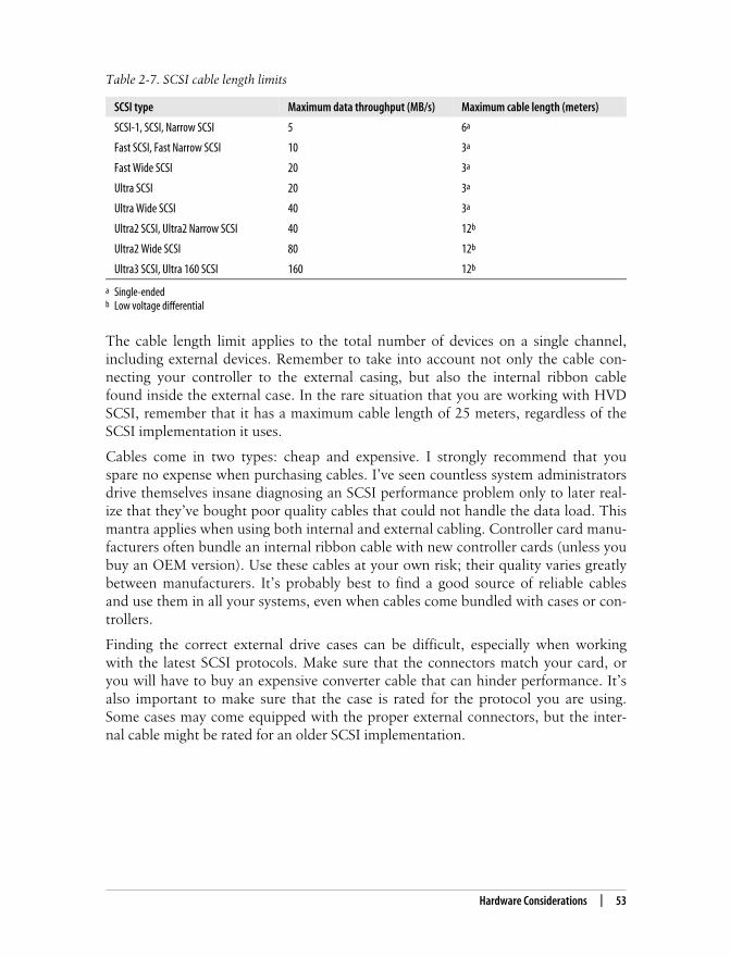
This is the Title of the Book, eMatter EditionCopyright © 2008 O’Reilly & Associates, Inc. All rights reserved.
Hardware Considerations | 53
The cable length limit applies to the total number of devices on a single channel,including external devices. Remember to take into account not only the cable con-necting your controller to the external casing, but also the internal ribbon cablefound inside the external case. In the rare situation that you are working with HVDSCSI, remember that it has a maximum cable length of 25 meters, regardless of theSCSI implementation it uses.
Cables come in two types: cheap and expensive. I strongly recommend that youspare no expense when purchasing cables. I’ve seen countless system administratorsdrive themselves insane diagnosing an SCSI performance problem only to later real-ize that they’ve bought poor quality cables that could not handle the data load. Thismantra applies when using both internal and external cabling. Controller card manu-facturers often bundle an internal ribbon cable with new controller cards (unless youbuy an OEM version). Use these cables at your own risk; their quality varies greatlybetween manufacturers. It’s probably best to find a good source of reliable cablesand use them in all your systems, even when cables come bundled with cases or con-trollers.
Finding the correct external drive cases can be difficult, especially when workingwith the latest SCSI protocols. Make sure that the connectors match your card, oryou will have to buy an expensive converter cable that can hinder performance. It’salso important to make sure that the case is rated for the protocol you are using.Some cases may come equipped with the proper external connectors, but the inter-nal cable might be rated for an older SCSI implementation.
Table 2-7. SCSI cable length limits
SCSI type Maximum data throughput (MB/s) Maximum cable length (meters)
SCSI-1, SCSI, Narrow SCSI 5 6a
a Single-ended
Fast SCSI, Fast Narrow SCSI 10 3a
Fast Wide SCSI 20 3a
Ultra SCSI 20 3a
Ultra Wide SCSI 40 3a
Ultra2 SCSI, Ultra2 Narrow SCSI 40 12b
b Low voltage differential
Ultra2 Wide SCSI 80 12b
Ultra3 SCSI, Ultra 160 SCSI 160 12b

This is the Title of the Book, eMatter EditionCopyright © 2008 O’Reilly & Associates, Inc. All rights reserved.
54 | Chapter 2: Planning and Architecture
Drives come in two sizes: 3.5” and 5.25”. The 5.25” drives can only be placed in5.25” bays. These drive bays are usually external, meaning that a plastic piece onthe front of the case can be removed to expose the drive. 5.25” bays are full-height(3.25”). Full-height (5.25”) drives are uncommon in today’s PC market. Youmight find very large-capacity drives that have this form factor, but most disks arehalf-height (1.625”) and have a width of 3.25”. These smaller drives can behoused in 5.25” drive bays by using extension brackets that are usually bundledwith cases. They can also be housed in 3.25” bays, which might be external orinternal. When buying cases, external bays refer to spots that can be accessedwithout opening the case. Internal bays refer to drive mounts that can be accessedonly when the case is opened.
Connectors
ATA cables use a standard 40-wire, 40-pin ribbon cable, while Ultra ATA (speeds of33 MB/s and above) uses a 40-pin, 80-wire cable (as shown in Figure 2-26). The con-nectors and cables might look identical, but you must use the 80-wire with UltraATA disks. Be sure to check the specifications when purchasing cables.
SCSI cables are much more confusing because SCSI cables have undergone moretransformations than ATA cables. In most cases, you will be using a 68-pin ribboncable for internal devices. Just make sure it’s rated for the bandwidth you’re using.Older external connectors have some variation (see Figure 2-27), but in most cases,68-pin high-density (HD) connectors are used. However, newer 68-pin very high-den-sity (VHD) connectors are making their way into the market. Decreasing the size ofexternal connectors has made it easier for SCSI controller manufacturers to housemultiple channels on a single card.
If you have different connectors on your controller card and your case, it’s easy tofind cables that can accommodate you. Check out http://www.scsipro.com for cus-tom SCSI cables.
Figure 2-26. ATA cables all have the same 40-pin connectors, but Ultra AT (speeds greater than 33MB/s) require newer 80-wire cables.
1
40-wire cable(IDE, EIDE, ATA)
4020 1 8040
80-wire cable(Ultra ATA 33, 66, 100)
40-pin connector

This is the Title of the Book, eMatter EditionCopyright © 2008 O’Reilly & Associates, Inc. All rights reserved.
Hardware Considerations | 55
Single connector attachment (SCA)
To facilitate hot-swap disks, IBM introduced the single connector attachment (SCA)for SCSI hard disks. SCA integrates data transfer, power, and configurable options(such as SCSI ID) on a single 80-pin connector, as shown in Figure 2-28. Drives areplugged into an SCA backplane that is then connected to the SCSI bus (usually viaSCSI ribbon cable) and the power supply. SCA drives are mounted in trays that slideinto the backplane and lock into place, leaving the other side of the disk tray accessi-ble from the outside of the case. These features make it easy to swap disks by elimi-nating the need to power down the system and dismantle the case.
Since its inception, SCA has been adopted by several manufacturers, and SCA-2 isthe current implementation standard. SCA drives tend to be slightly more expensivethan standard drives. Cases with SCA backplanes also run on the expensive side, butSCA is a necessity for any system that needs hot-swap capability because SCA isdesigned to allow power-on disk swapping. Recently, SCA chassis that fit into standard
Figure 2-27. Most SCSI controllers use 68-pin high-density connectors for external connections.You may encounter some older connectors as well.
Figure 2-28. SCA disks use an 80-pin connector that facilitates data transfer, power, andconfiguration parameters.
50-pin Centronics(8 bit, SCSI-1, 5MB/s)
25-pin DB25(8 bit, 5MB/s, Apple)
50-pin HD50(8 bit, SCSI-2, 10MB/s)
68-pin high-density (HD)(16 bit, Wide/Wide Ultra, 40MB/s)
68-pin very high-density (VHD)(16 bit, Ultra2, Ultra 160/320, 320MB/s)
Cable/Backplane side
Device side
Advanced grounding contacts
Actual drive
Connector that's usually part of adisk enclosure or case
Connectors are 80 pins-and supply power

This is the Title of the Book, eMatter EditionCopyright © 2008 O’Reilly & Associates, Inc. All rights reserved.
56 | Chapter 2: Planning and Architecture
desktop cases have surfaced. Enlight Corporation (http://www.enlightcorp.com) man-ufactures a module that fits into three 5.25” drive bays. It supports up to five SCAdisks and connects to an internal SCSI controller. Rackmount case makers also tendto sell custom drive cases that come equipped with an SCA backplane.
Individual adapter modules that allow the use of a single SCA disk with standard 68-pin SCSI cabling and power supply connection are also readily available. I’ve hadmixed results using them, ranging from problem-free performance to SCSI channelsrunning at less than optimal speeds. You will probably also have mixed results, butthey do offer a pretty cheap way to get SCA functionality, especially on systems withonly a couple of disks. Most cases support a minimum of five or six disks and arevery pricey.
Power
Finally, make sure you have an adequate power supply in all your cases, whetherthey are dedicated drive cases or contain a system and disks. Most cases provide justenough internal power connectors so that the power supply cannot be overloaded.You can purchase power splitters if you run out of connectors, but remember thatoverloading a power supply can lead to fried hardware. If you find that you havemore peripherals than power, you should considering upgrading your power supply.Most cases can be custom ordered with power supplies of up to 450 watts for a mini-mum of extra cash.
Making Sense of It AllIn the final section of this chapter, I’d like to present an example RAID system that Ibuilt using parts available at most decent computer stores and online retailers.
The system in question was designed to replace a medium-volume web server thathosts content for video game enthusiasts. The original server was homegrown andquickly became inadequate as the site grew in popularity and moved out of itsowner’s workplace into a collocation facility. Connecting the system to a larger net-work pipe solved many of its initial problems, but eventually, the hardware itselfbecame overworked.
The site is mostly static, except for a few moderators who post new articles andreviews each day. It’s essential that the site have a 24 × 7 uptime, so RAID-0 is out ofthe question. And with my budget, RAID-1 wouldn’t work either, because the sitefrequently distributes large video clips and demos of upcoming games. I simplycouldn’t afford the extra disks RAID-1 would require. That left RAID-5 as the bestoption.
In building the new RAID system, I needed to select a motherboard first because theold 32-bit PCI board was causing most of the performance problems on the originalserver. Because I was interested in high performance, I chose a motherboard that had

This is the Title of the Book, eMatter EditionCopyright © 2008 O’Reilly & Associates, Inc. All rights reserved.
Making Sense of It All | 57
two 64-bit PCI slots. Each of these 64-bit slots had a dedicated data bus with athroughput of 533 MB/s. (Remember that 64-bit PCI boards run at 66 MHz [66.6million cycles per second * 8 bytes per cycle = 533 MB/s]). The remaining expansionslots are 32-bit and share a data bus with a throughput of 133 MB/s. The 32-bit buswouldn’t be used for anything except a low-end video card (for local administra-tion), although in the future, a network card might be installed so that the systemcould be connected to a private administrative network.
In the first 64-bit PCI slot, I installed a high-speed networking card, which shouldalleviate any networking bottlenecks that the site was experiencing when it was usinga 100-megabit Ethernet card. In the second slot, I installed a quad-channel UltraSCSI 160 controller, giving me to a total disk bus throughput of 480 MB/s (3 * 160MB/s). The unused bandwidth would help ensure that I didn’t saturate the 533 MB/sdata bus, while allowing for occasional burst rates that exceed the specifications ofmy disks and controller.
I found some reasonably priced hard disks that supported a sustained data rate of 40MB/s and purchased a few external cases. Therefore, I didn’t need to worry aboutcramming everything into a single desktop case. I knew that even the biggest desk-top cases house only 7 or 8 disks, and that wouldn’t allow me to take full advantageof my controller (480 MB/s ÷ 40 MB/s = 12 disks). After doing some thinking, Idecided to purchase twelve drives, and I connected three of them to each controllerchannel. The drives are housed in the external cases I bought, externally connectedto individual channels.
Although the average disk throughput was 40 MB/s, the manufacturer’s specifica-tions indicate that burst rates higher than that are common. Because I was usingRAID-5, I could configure the array so that the system alternated between SCSIchannels during I/O operations. That would help offset the potential for bottleneckson an individual channel when the disks burst higher than 40 MB/s.
Once all the equipment (see Figure 2-29) was connected, I was left with three driveson each channel, with an aggregate disk bus throughput of 480 MB/s. That left someoverhead on my data (PCI) bus to be safe, but didn’t waste much of its potential,since I expected the disks would often outperform the 40 MB/s data rate by a smallamount. I didn’t need to worry about the graphics adapter or network cards interfer-ing with disk throughput, either, because they were installed on separate data buses.
Hardware is always changing and the equipment you buy doesn’t always meet yourexpectations, so it’s always a good idea to do research before building or purchasingany system.
As an example of what can go wrong, a former collegue recently told me that he hadto argue with his vendor in order to get a system with multiple SCSI backplanes. Hehad ordered a dual-channel RAID controller in a rackmount case with eight harddisks. But the vendor had designed the system so that there was only a single SCA

This is the Title of the Book, eMatter EditionCopyright © 2008 O’Reilly & Associates, Inc. All rights reserved.
58 | Chapter 2: Planning and Architecture
backplane. This meant that all of his data would be travelling over a single SCSIchannel and that the second channel would be wasted. The vendor offered theoption of adding an external disk-only case for the second channel, but my colleaguefound that unfeasible due to the the high price of server colocation it added. In theend, my collegaue had to swap his components into a new case with two back-planes. The vendor ate the cost, but it took an extra week to get the system online.
Also, remember compatibility issues. I recommend checking relevant mailing listsand web sites to make certain that your disk controllers will work properly with yourmotherboard and network controller.
Figure 2-29. My web server contains a quad-channel SCSI controller. Three disks are connected toeach channel.
Motherboard
PCI (32 bit)PCI
(64 bit)
Controller
C DA B
Shared databus
A B C D
External disk cases

This is the Title of the Book, eMatter EditionCopyright © 2008 O’Reilly & Associates, Inc. All rights reserved.
59
Chapter 3 CHAPTER 3
Getting Started:Building a Software
RAID
Before plunging into this chapter, you should be familiar with the process of build-ing and installing a new kernel. If you have never done this before, I strongly suggestthat you read Brian Ward’s “The Linux Kernel HOWTO” (http://www.tldp.org/HOWTO/Kernel-HOWTO.html), which is available at any Linux DocumentationProject mirror and is likely included with your distribution. If you prefer books toonline documentation, then I’d recommend you pick up a copy of Running Linux(O’Reilly). Chapter 7 of that book offers an excellent tutorial on managing the ker-nel. To become comfortable installing a new kernel, I suggest you make some simplechanges first.
A good start would be to eliminate some loadable modules from your kernel andinclude those subsystems statically. Most distributions set up major system peripher-als as loadable modules, rather than compiling them statically into the kernel. Net-work drivers are a good example of kernel subsystems that are often installed, bydefault, as loadable modules. The sheer number of available network hardware con-figurations makes this the only efficient way to circulate network-enabled Linux dis-tributions. So, in order to maintain compatibility with as many systems as possible,distributors such as Red Hat, Mandrake, and SuSE automatically load modulesappropriate to your system at boot time, while installing a stock kernel with supportfor loadable modules. Using modules also helps conserve system memory by reduc-ing the size of the running kernel. Modules can be unloaded when they are no longerneeded, freeing up additional system resources.
While this is a completely viable way to set up a Linux machine, I tend to feel that amonolithic kernel, a kernel without modules, is more appropriate for system stabil-ity and is essential for servers. Loadable modules leave room for uncertainty duringsystem initialization and are therefore best left to desktop machines and novices.Since servers typically perform specific and dedicated services, a monolithic kernelsuits them best. Once you are comfortable recompiling the kernel and reconfiguringyour boot manager, you can begin adding support for RAID.

This is the Title of the Book, eMatter EditionCopyright © 2008 O’Reilly & Associates, Inc. All rights reserved.
60 | Chapter 3: Getting Started: Building a Software RAID
This chapter will guide you through implementing a software RAID by explaininghow to:
• Enable kernel RAID features
• Download and install software RAID utilities
• Partition hard disks
• Create an array
Kernel ConfigurationSoftware RAID support must be enabled in the kernel before you can create anyarrays. This generally means recompiling your kernel, configuring your boot loader(such as LILO or GRUB) to load the new kernel, and, finally, restarting the systemwith the new kernel.
A Brief History LessonAlthough kernels prior to 2.0.35 shipped with some RAID support, it wasn’t until therelease of 2.0.35 that support for RAID-1, RAID-4, and RAID-5 became available.The multiple devices (md) driver that provides kernel RAID support is currently atversion 0.90. The latest stable kernels in the 2.0 and 2.2 series ship with an outdatedversion (0.36) of the software RAID driver. Patches for the 0.90 code are available forthese older kernels (see the sections below on “Kernel 2.2” and “Kernel 2.0”). Ker-nels prior to 2.0.35 ship with version 0.35 of the md driver and should not be used,except if you absolutely have to keep them in operation for legacy reasons.
The 0.90 code was finally merged with the kernel source tree during the 2.3 develop-ment phase, so 2.4 ships with the latest RAID code. So will all subsequent stable anddevelopment kernels. In general, it’s best to run at least a 2.4 series kernel whenusing software RAID, or a 2.2 kernel with the proper RAID patches applied. Usingthe old 0.36 driver is not recommended.
Along with drivers to provide software RAID for Linux, a set of utilities for manag-ing, configuring, and tuning software arrays has emerged. These utilities, collectivelycalled the RAID Tools (raidtools is the package name), are maintained by Ingo Mol-nar and Erik Troan of Red Hat and are now included with many major distribu-tions. Molnar also served as the primary developer and maintainer of the softwareRAID subsystem from version 0.36 through 0.90’s integration into the stable kerneltree. Today, he shares that responsibility with Neil Brown, a software engineer at theUniversity of New South Wales. Brown also contributed many performance and reli-ability-related patches before becoming an official maintainer. In August 2001,Brown began work on his own software RAID utilities for Linux. His multiple devicesadministration (mdadm) program is a great alternative to the slightly aging raidtools.Both packages are covered in this book. I recommend using mdadm when possible.

This is the Title of the Book, eMatter EditionCopyright © 2008 O’Reilly & Associates, Inc. All rights reserved.
Kernel Configuration | 61
Many other programmers have contributed to the md driver since its original devel-opment. Marc Zyngier wrote the original implementations of linear mode and RAID-0, along with the predecessor to raidtools. Miguel de Icaza helped develop the firstimplementation of RAID-1 and wrote the first version of raidtools. Gadi Oxmanwrote the first 0.90 implementation of RAID-5.
Kernel 2.4As of version 2.4, software RAID has its own subsection in the kernel configuration(in previous versions, options were found under the Block Devices submenu). TheMulti-device Support (RAID and LVM) submenu contains all the configurationoptions for software RAID. The first option, CONFIG_MD, is a configuration switch thatreveals options for RAID and Logical Volume Management (LVM). After selectingCONFIG_MD, choose CONFIG_BLK_DEV_MD, which allows the kernel to address multiplephysical devices through a single logical device (see Figure 3-1). CONFIG_BLK_DEV_MDprovides the foundation for the md driver and needs to be enabled on every systemthat uses software RAID, regardless of which RAID level is implemented.
In order to successfully build a software RAID device, one of the available RAID lev-els must also be enabled. The following kernel directives enable support for specificRAID levels:
CONFIG_MD_LINEARCONFIG_MD_RAID0CONFIG_MD_RAID1CONFIG_MD_RAID5
CONFIG_MD_LINEAR and CONFIG_MD_RAID0 enable support for the non-RAID methods ofdisk grouping supported by the Linux kernel. CONFIG_MD_RAID1 provides support for
Figure 3-1. Enabling kernel RAID support.

This is the Title of the Book, eMatter EditionCopyright © 2008 O’Reilly & Associates, Inc. All rights reserved.
62 | Chapter 3: Getting Started: Building a Software RAID
data redundancy through disk mirroring. Finally, CONFIG_MD_RAID5 enables supportfor both RAID-4 and RAID-5 layouts. The choice between using RAID-4 or RAID-5is made later, when creating an array. If you plan to experiment with more than oneof the available RAID levels, or if you are still unsure which RAID level you plan toimplement, you can enable all four levels, rather than compiling a separate kernel foreach (Figure 3-2) or recompiling your kernel each time you wish to experiment withanother level. This is extremely useful during testing. When you’re ready to go intoproduction, simply rebuild the kernel with only the RAID levels you need. RAIDsupport is also available as loadable kernel modules.
You will also notice an option for Multipath I/O support (CONFIG_MD_MULTIPATH).This newer feature of the md driver allows the addressing of a single physical diskusing multiple I/O paths (controllers or channels). So if one I/O path becomesunavailable, the disk is still accessible. Multipath I/O support is not covered in thisbook.
Once you have added the desired options to your kernel configuration, compile thenew kernel with support for software RAID.
# make dep# make bzImage
The new kernel should be located at .../arch/i386/boot/bzImage (for i386-based sys-tems), under the kernel source directory. If you are using a non-Intel machine, lookfor the compiled kernel image in the directory that is appropriate for your architec-ture (.../arch/sparc/boot/ on SPARC systems, for example).
Figure 3-2. Enable support for specific RAID levels.

This is the Title of the Book, eMatter EditionCopyright © 2008 O’Reilly & Associates, Inc. All rights reserved.
Kernel Configuration | 63
Installing the new kernel
Linux kernels are traditionally stored in the /boot directory (usually a dedicated parti-tion) or occasionally in the root directory. Copy the new kernel to the /boot direc-tory, or to the directory where you normally keep your kernels, if you have anonstandard situation. The following example works on i386-based systems.
# cp arch/i386/boot/bzImage /boot/bzImage.raid# cp System.map /boot/
You can name the kernel anything you like, but I find it helpful to name it some-thing descriptive. Others prefer to include the version number in the filename. Next,add an entry for the RAID-enabled kernel to the boot loader configuration.
On systems using the Linux Loader (LILO), /etc/lilo.conf contains information aboutwhich kernel image is loaded during the system initialization. LILO users might addthe following entry to /etc/lilo.conf:
image=/boot/bzImage.raid label=linux-raid read-only root=/dev/sda1
Make sure that you enter the correct root device, if it is not /dev/sda1. Either placethis stanza before all the others listed in /etc/lilo.conf, or use the default global key-word to specify which kernel to boot (see the lilo.conf manual page for furtherdetails). You can also simply select the Linux-raid kernel from the LILO prompt dur-ing startup and avoid changing the default.
# liloAdded linux-raid *Added linux-orig# shutdown -r now
You can also use lilo -R to specify which kernel to load when the system restarts(after you run lilo to rebuild the boot sector). In the following example, the Linux-raid kernel will be loaded the next time the system restarts, even though it is not thedefault kernel listed in /etc/lilo.conf.
# liloAdded linux-raidAdded linux-orig *# lilo -R linux-raid# shutdown -r now
lilo -R works for only one subsequent reboot. So, once you are satisfied with the newkernel, remember to change the default in /etc/lilo.conf or rearrange the stanzas.

This is the Title of the Book, eMatter EditionCopyright © 2008 O’Reilly & Associates, Inc. All rights reserved.
64 | Chapter 3: Getting Started: Building a Software RAID
Some distributions are beginning to use the Grand Unified Bootloader (GRUB)instead of LILO. GRUB users can add lines like the following to their /boot/grub/grub.conf file:
title Linux RAID (2.4.18) root (hd0,0) kernel /bz.2418 ro root=/dev/sda2
This entry will load the kernel found at /boot/bz.2418 on the first hard disk (hd0,0)using a root device of /dev/sda2, mounted initially as read-only. By default, GRUBwill boot the first entry it finds in grub.conf, so you could either place the lines aboveas the first entry or change the default parameter to reflect the correct kernel.
System initialization
When the system restarts, a message indicates that the md driver has initialized. EachRAID level compiled into the kernel is listed, along with information about thedriver. On a system with support for all available RAID levels, the following messageshould appear:
md driver 0.90.0 MAX_MD_DEVS=256, MD_SB_DISKS=27linear personality registeredraid0 personality registeredraid1 personality registeredraid5 personality registered
If your system boots faster than you can read the messages, use the dmesg commandto examine boot messages after the system has initialized. dmesg displays the kernelring buffer, allowing users to examine important kernel messages that they mighthave missed during kernel initialization. The kernel ring buffer stores, in memory,messages about the current state of the running kernel. Some distributions arealready preconfigured to dump these messages to a file after the system boots, butyou can simply redirect the output to a file (dmesg > boot.messages) or pipe it into apager (dmesg | less) at your whim. Messages returned by dmesg might look a littlebit different from their appearance while the system is booting, but the same infor-mation is there:
# dmesg | grep mdmd: linear personality registered as nr 1md: raid0 personality registered as nr 2md: raid1 personality registered as nr 3md: raid5 personality registered as nr 4md: multipath personality registered as nr 7md: md driver 0.90.0 MAX_MD_DEVS=256, MD_SB_DISKS=27
When the md driver initializes, its version is displayed (0.90.0, in this case). MAX_MD_DEVS indicates that the number of RAID devices is limited to 256 (with devices filesnamed /dev/md[0-255]), and MD_SB_DISKS indicates that each software array is lim-ited to 27 member disks. However, by building hybrid arrays, users can move wellbeyond this limit. Hardware limitations will become an issue long before you reachthe limits of the md driver.

This is the Title of the Book, eMatter EditionCopyright © 2008 O’Reilly & Associates, Inc. All rights reserved.
Kernel Configuration | 65
The kernel also registers each RAID level, or personality. In this case, the kernel con-tains support for linear mode, RAID-0, RAID-1, and RAID-4/5. If RAID support wascompiled as loadable kernel modules, these initialization messages will not appear,but you should see them later in your system logs when those modules are inserted.These messages will be reported (like all md driver messages), using the kern facility,starting at the info level.
Please note that as the system remains running, the kernel ring buffer will begin toexpunge old messages. So be certain to examine it soon after booting if you need toview information generated by the boot process. Most distributions are also precon-figured to place this information in /var/log/messages after the system boots. Pleasebe aware that some distributions also come configured with an /etc/syslogd.conf thatgenerates a misnamed file called /var/log/boot.log, using the log facility local7. Thisfile (and any files generated using local7) contains messages from system initializa-tion scripts (rc), not kernel initialization messages. Kernel messages are captured byklogd and dumped to syslogd once klogd has executed. In most default configura-tions, you will find messages about the md driver in /var/log/messages, includingthose dumped from the kernel ring buffer by klogd. Chapter 7 covers system loggingand the md driver in further detail.
If RAID-5 is supported, the kernel will also optimize the XOR routines used for par-ity checksum in a RAID-5. A message indicating that the test was performed is dis-played, along with its results:
raid5: measuring checksumming speed 8regs : 1835.600 MB/sec 32regs : 871.600 MB/sec pIII_sse : 2021.200 MB/sec pII_mmx : 2277.200 MB/sec p5_mmx : 2386.000 MB/secraid5: using function: pIII_sse (2021.200 MB/sec)
Since different i386-based processor architectures implement different ways to per-form the necessary XOR operations, Linux needs to determine which one is the mostefficient for a particular system in advance. Notice that in this example, the fastestchecksum operation was not chosen. On systems that support Streaming SIMDExtensions (SSE), that choice is selected because of its ability to circumvent the L2cache and perform operations in parallel (see /usr/src/linux/include/asm-i386/xor.h).This functionality improves the performance of checksum operations. Informationabout checksum algorithms is also recorded in the kernel ring buffer.
After the system restarts, examining /proc/mdstat will also show that the RAID sub-system was successfully initialized with support for linear mode, RAID-0, RAID-1,and RAID-4/5.
# cat /proc/mdstatPersonalities : [linear] [raid0] [raid1] [raid5]read_ahead not setunused devices: <none>

This is the Title of the Book, eMatter EditionCopyright © 2008 O’Reilly & Associates, Inc. All rights reserved.
66 | Chapter 3: Getting Started: Building a Software RAID
See the section “Examining Arrays Using /proc/mdstat,” later in this chapter, formore information.
Patching Older KernelsWorking with 2.0.X and 2.2.X kernels can be extremely confusing because of the lay-out and documentation for the available patches. Most people have a lot of troublesifting through all the old and erroneous information relating to these kernel ver-sions and their RAID implementations. While RAID support is included with 2.0.Xand 2.2.X series kernels, the most recent drivers are not distributed with the kernelsource code, and patches should be applied when possible. There are also knownproblems with RAID-5 on 2.2 and 2.0 kernels, so if you want to use RAID-5, youshould upgrade to at least a 2.4 kernel.
Kernel 2.2
When working with 2.2 series kernels, I strongly recommend that you upgrade to thelatest RAID code (0.90). The 0.90 code is available as a patch to the kernel andshould be applied before any attempt to build new arrays. As a general principle, youshould always be working with version 0.90 (or later) of the RAID code. You canexamine the file .../linux/include/linux/md.h to determine which version of the RAIDcode is present on 2.0 and 2.2 series kernels. Version information is located near thebeginning of the file:
[...]#define MD_MAJOR_VERSION 0#define MD_MINOR_VERSION 36#define MD_PATCHLEVEL_VERSION 6[...]
This 2.2 kernel has version 0.36.6 of the RAID subsystem; therefore, a patch shouldbe applied. If .../linux/include/linux/md.h is either empty or missing, your kernel isprobably already patched to version 0.90. Instead, check the file .../linux/include/linux/raid/md.h for the version information. Note the extra subdirectory named raidin the path. As the size of RAID code grew, a subdirectory was created to better orga-nize its components.
Patches for the 2.2 kernel are available at http://people.redhat.com/mingo/raid-patches/. A patch for the most recent sublevel release of 2.2, as well as patches for afew prior 2.2 sublevel releases, should be available at this site. Grab the one for thespecific sublevel release with which you are working. If a patch for that particularsublevel release is unavailable, I recommend upgrading to the most recent 2.2 releaseand using the matching RAID patch.
For example, if you are working with kernel 2.2.20, download the patch http://people.redhat.com/mingo/raid-patches/raid-2.2.20-A0. Apply the raid-2.2.20-A0

This is the Title of the Book, eMatter EditionCopyright © 2008 O’Reilly & Associates, Inc. All rights reserved.
Kernel Configuration | 67
patch to your 2.2.20 kernel, using the -p1 flag to indicate that you are in the rootdirectory of the source tree:
# cd /usr/src/linux-2.2.20# patch -s -p1 < /usr/src/patches/raid-2.2.20-A0
Passing the -s flag to patch invokes quiet mode. If patch is successful, no output itreturned. If an error was encountered, then patch will output a list of reject files thatcontain more detailed information about the errors. If you encounter errors, it’s pos-sible that a faulty, or untested, patch was released. Try throttling your kernel back-ward one revision (to 2.2.19, in this case), download a new patch, and reapply it.When the problem is eventually corrected, you can safely upgrade and repatch. Youcan, alternatively, examine the reject files and attempt to manually fix problems thatpatch encounters. If you choose not to use quiet mode, then patch will return a list offiles that have been successfully patched, in addition to the names of any reject filesgenerated.
Remember that new patch files and kernels are released often, so the filenames usedthroughout this book may differ slightly from the ones you encounter when down-loading patches. The locations of important kernel patches will also inevitably changeas kernel maintainers change employers and as subsystems change maintainers.
When working with kernel patches, it’s a good idea to apply them to a clean,unpatched kernel. Moshe Bar has written an excellent article for BYTE magazine thatexplains the implications of kernel source trees and applying patches to clean ker-nels (http://www.byte.com/documents/s=2470/byt1012259408690/0204_bar.html).
As in 2.4 kernels, RAID support must be enabled during kernel configuration of 2.2kernels. During this earlier phase of RAID development, the RAID subsystem did nothave its own submenu. Instead, RAID configuration options were put in the BlockDevices submenu. Simply enable Multiple Devices Driver Support (CONFIG_BLK_DEV_MD) and at least one RAID level (see Figure 3-3).
Figure 3-3. Enable support for Multiple Devices and at least one RAID level.

This is the Title of the Book, eMatter EditionCopyright © 2008 O’Reilly & Associates, Inc. All rights reserved.
68 | Chapter 3: Getting Started: Building a Software RAID
If you plan to experiment with different RAID levels, simply enable all of them.Under 2.2, the various RAID levels can also be built as loadable kernel modules. Youmight also notice some other options that provide additional features. The first,Autodetect RAID Partitions (CONFIG_AUTODETECT_RAID), allows the kernel to automati-cally activate arrays when the system boots. Originally, RAID devices were startedeither manually at the command line or by system initialization (rc) scripts.
Autodetection examines the RAID superblock (see “The RAID Superblock” section,later in this chapter) on hard disks to determine which disks are members of arraysand then to activate them. It is safe to leave RAID autodetection enabled. On newerkernels, autodetection is standard and therefore no longer appears as an option.
Translucent Mode (CONFIG_MD_TRANSLUCENT) and Hierarchical Storage ManagementSupport (CONFIG_MD_HSM) were experimental options that appeared in the 2.2 kernel,but were never developed. They no longer appear in later kernels and should be dis-abled when working with any kernel that advertises them as features.
Kernel 2.0
As I’ve mentioned several times earlier in this chapter, kernels earlier than 2.2 arebest not used for software RAID. Software RAID under 2.0 kernels is especially con-fusing. Patch files are no longer maintained, older utilities are needed to managedevices, and both patches and tools are kept in an area of kernel.org that is not main-tained. So it’s best to avoid using software RAID with 2.0 kernels, unless there areextenuating circumstances. If you must work with a 2.0 kernel, I strongly recom-mend upgrading to the latest kernel prior to using software RAID. Usable patches areavailable only for kernels newer than 2.0.35. It’s a bad idea to even attempt using akernel older than this.
Download the most recent 2.0 kernel patch from ftp://ftp.kernel.org/pub/linux/daemons/raid/alpha/. Notice that this directory contains files for both 2.0 and 2.2kernels. Use only 2.0 kernel patches from this directory. (Patches for 2.2 should beobtained as described in the previous section, “Kernel 2.2.”)
Note, though, that if you were using kernel 2.0.39, you would need to downloadraid0145-19990824-2.0.37.gz. As of this writing, no patches specific to kernels laterthan 2.0.37 were available. The 2.0.37 patch should apply without severe problems.But if you find yourself in a situation in which a patch doesn’t match your kernelsublevel version, or if you encounter problems while patching or compiling a 2.0 ker-nel, you should work with the kernel that matches the most recent patch. At worst,you will be forced to use a kernel that is one or two sublevel revisions behind, andeventually a newer patch will be released and you can upgrade.
To be on the safe side, I’m going to unroll a 2.0.37 kernel and apply this patch,rather than risk using a 2.0.39 kernel that might present problems during compila-tion or at runtime.

This is the Title of the Book, eMatter EditionCopyright © 2008 O’Reilly & Associates, Inc. All rights reserved.
Kernel Configuration | 69
# cd /usr/src/linux-2.0.37# patch -s -p1 < /usr/src/patches/raid0145-19990824-2.0.37
With 2.0.37, the patch returns no errors. A 2.0 kernel using the 0.90 RAID sub-system is now ready for compilation. Enable RAID features under the Floppy, IDE,and other block devices submenu during configuration (see Figure 3-4). First, enableMultiple Devices Support (CONFIG_BLK_DEV_MD) and then any RAID you need. It issafe to leave Autodetect RAID Partitions (CONFIG_AUTODETECT_RAID) activated, butleave Translucent Mode (CONFIG_MD_TRANSLUCENT) and Hierarchical Storage Manage-ment Support (CONFIG_MD_HSM) disabled (see the previous section, “Kernel 2.2”).
Summary of Kernel UpgradesIn summary, the latest version of the software RAID (multiple devices) driver forLinux is 0.90. However, kernels 2.0 and 2.2 were distributed with an older version(0.36) of the driver. If you are using kernel 2.4 or later, then you already have the lat-est driver, but you might wish to check the web pages of both Ingo Molnar (http://people.redhat.com/mingo/raid-patches/) and Neil Brown (http://www.cse.unsw.edu.au/~neilb/patches/linux-stable/) for performance and reliability patches that are waitingto make it into the next kernel revision.
When working with 2.0 and 2.2 kernels, it’s essential to upgrade to the 0.90 driverwhenever possible. Follow the steps described in this section to download the appro-priate patch and apply it to your kernel. If you encounter problems during this pro-cess, you might need to try patching different kernel sublevel releases until you findone that patches without errors. Use kernels that do not patch properly at your ownrisk.
Figure 3-4. Under 2.0 kernels, RAID functions are configured under the Floppy, IDE, and otherblock devices submenu.

This is the Title of the Book, eMatter EditionCopyright © 2008 O’Reilly & Associates, Inc. All rights reserved.
70 | Chapter 3: Getting Started: Building a Software RAID
If, for one reason or another, you are working with a 2.0 or 2.2 kernel and cannotupgrade to the 0.90 RAID, than you are in the unfortunate circumstance of having touse the very outdated 0.36 driver. The 0.36 driver is not compatible with the newer0.90 driver, and you will need to use an older version of the raidtools package tomanage arrays created for the 0.36 driver. Only four software arrays are supportedunder version 0.36.
Working with Software RAIDThe raidtools package, also maintained by Ingo Molnar, provides a set of utilities forcreating and managing software arrays. raidtools has been the standard softwareRAID management package for Linux since the inception of the software RAIDdriver. Over the years, raidtools has proven cumbersome to use, mostly because itrelies on a configuration file (/etc/raidtab) that is difficult to maintain, and partlybecause its features are limited. In August 2001, Neil Brown released an alternative.His mdadm package provides a simple, yet robust way to manage software arrays.mdadm is now at version 1.0.1 and has proven quite stable after its first year of devel-opment. It has received a positive response on the Linux-raid mailing list and willlikely become widespread in the future. The rest of this chapter will provide you withexamples of building and managing arrays, using the raidtools package, as well asmdadm.
raidtoolsraidtools provides a small, simple command set that allows administrators to create,activate, and stop software arrays. Each array managed by the system is defined in aglobal configuration file (/etc/raidtab) that describes which physical disks are mem-bers of each array. /etc/raidtab also contains metadata about every array, such as itsRAID level and failover capabilities. The commands included with the raidtoolspackage use the information in /etc/raidtab to interface with arrays.
There are two notable versions of raidtools. Version 0.90 is the most recent imple-mentation, and the only one being maintained. It should be used only in conjunc-tion with the 0.90 driver. An older version (0.42) of raidtools is also still available.This version should only be used when working with older systems that still use the0.36 software RAID driver. Never use raidtools with the wrong driver!
Also included with raidtools are sample configuration files and documentation (man-ual pages and cookbooks). Unfortunately, much of the documentation is seriouslyoutdated, sometimes by a factor of years. Adhering to the open source philosophythat “old documentation is better than no documentation,” a lot of outdated infor-mation is included with the raidtools package. It’s probably best to double-check aLinux Documentation Project mirror for the most recent information and consultadditional reference material and mailing lists in lieu of relying on the documenta-tion in the package.

This is the Title of the Book, eMatter EditionCopyright © 2008 O’Reilly & Associates, Inc. All rights reserved.
Working with Software RAID | 71
As of this writing, raidtools-1.0 has been released in a limited capacity. It can befound in Red Hat 8.0 and will likely become pervasive during the next few months. Itfixes several minor bugs and can be used as a replacement for raidtools-0.90.Chapter 4 presents more information about raidtools-1.0 and some new utilitiesincluded with it.
raidtools-0.90
Most modern Linux distributions ship with the raidtools package. You can installthem from your installation media or download them from your vendor. In a RedHat CD directory, for example, issue the following command:
# rpm -ihv ./raidtools-0.90-20.i386.rpm
Debian users can use apt-get to install the raidtools:
# apt-get install raidtools2
Note that under Debian, raidtools2, NOT raidtools, provides the 0.90 raidtools pack-age. Please be certain you have the proper package installed.
You can also download the source code and compile the package yourself. The mostrecent version is available at ftp://ftp.kernel.org/pub/daemons/raid/alpha. As of thiswriting, the most recent version is ftp://ftp.kernel.org/pub/linux/daemons/raid/alpha/raidtools-19990824-0.90.tar.gz. You might be aware that a seemingly newer versionis available from http://people.redhat.com/mingo/raidtools/. There are several knownproblems with this version (raidtools-20010914), including its lack of a key manage-ment utility (raidsetfaulty). Use this version at your own risk. The raidtools packageshould compile without problems on any recent system, though it does require thepopt libraries. There are currently no notable configuration options. Download andunpack the archive.
# cd /usr/src/raidtools-YYYYMMDD# ./configure# make install
Compilation will leave you with several executables. Of particular note are mkraid,used to create new arrays, and raidstart, used to activate arrays that have alreadybeen initialized with mkraid. Installation will copy binaries to /sbin and create sym-bolic links that invoke specific functions for each utility. raidstop, for example, issimply a symbolic link that causes raidstart to invoke a case switch based on thecommand line. Manual pages are also installed. Chapter 4 covers each commandincluded with the raidtools package in detail.
At the time of this writing, version 1.0 of raidtools has just appeared in Red HatLinux 8.0. Version 1.0 of raidtools corrects the issues associated with raidtools-20010914 and includes some major improvements, such as bug fixes and a couple ofnew utilities. lsraid will allow you to query arrays and member disks. It will even letyou generate an /etc/raidtab file by querying a running array. raidreconf allows users

This is the Title of the Book, eMatter EditionCopyright © 2008 O’Reilly & Associates, Inc. All rights reserved.
72 | Chapter 3: Getting Started: Building a Software RAID
to add (or remove) disks to a RAID-0 or RAID-5, usually without data loss. Althoughthese utilities are somewhat new, I’ll discuss them throughout this book, since theyare particularly useful and will more than likely become widespread.
/etc/raidtab
/etc/raidtab is raidtools’ primary configuration file. /etc/raidtab provides a functionsimilar to /etc/fstab. It provides the kernel with a description of each software RAID,including its RAID level and a list of member disks. All RAID devices must have anentry in /etc/raidtab to be created or activated using raidtools.
Users create /etc/raidtab by hand, using any text editor. Once /etc/raidtab is createdand contains configuration information about arrays, the mkraid command can beused to construct an array based on the parameters defined in /etc/raidtab. mkraidwill complain if it cannot find a valid file at /etc/raidtab. This process is similar to cre-ating the boot configuration file /etc/lilo.conf and consequently running /sbin/lilo torebuild the boot block.
Here is a typical /etc/raidtab that describes a RAID-0 with two ATA componentdisks:
raiddev /dev/md0raid-level 0persistent-superblock 1chunk-size 64
nr-raid-disks 2nr-spare-disks 0
device /dev/hda1raid-disk 0
device /dev/hdb1raid-disk 1
Each array begins with a raiddev entry, followed by a list of array properties and anentry for each array member. A valid entry in /etc/raidtab must contain at least adefined raid-level, a chunk-size, the total number of raid disks (nr-raid-disks) andtwo device/raid-disk pairs. chunk-size is a bit counterintuitive because it appliesonly to arrays that support disk striping (RAID-0, RAID-4, and RAID-5), yet it isrequired for any array you define in /etc/raidtab. That’s because the utilities in theraidtools package (mkraid, most notably) check for a chunk-size even if the definedRAID level doesn’t support one. So when you work with linear mode or RAID-1, forexample, you must provide a chunk-size, even though it’s technically only a place-holder.
There are no global options in /etc/raidtab. Each section, or stanza, applies to the lastparsed raiddev entry. Once an array is defined, it may be included as a member disk

This is the Title of the Book, eMatter EditionCopyright © 2008 O’Reilly & Associates, Inc. All rights reserved.
Working with Software RAID | 73
in a subsequent array section. This allows you to combine multiple arrays into ahybrid array (as in RAID-10, for example).
Chapter 4 provides details about each /etc/raidtab parameter.
raidtools-0.42
It’s unlikely that you will be able to locate a package file for this outdated version ofraidtools. So, in most cases, you will be stuck compiling the tools yourself. Down-load version 0.42 of the raidtools (ftp://ftp.kernel.org/pub/linux/daemons/raid/raidtools-pre3-0.42.tar.gz) and unpack it.
One important caveat when working with this version is that it requires a patchedkernel to compile. By default, the configure command assumes that your kernel is in/usr/src/linux, but you can change that by using the --with-linux parameter.
# cd /usr/src/raidtools-0.42# ./configure --with-linux=/usr/src/linux-2.0.37# make# make install
Installation will leave you with an older version of mkraid, as well as several depre-cated utilities that are used to start (mdrun), stop (mdstop), and manage (mdcreate,ckraid) arrays. Manual pages are also installed by default.
Debian users can install version 0.42 of raidtools using apt-get:
# apt-get install raidtools
The rest of this chapter covers the current version of raidtools and the md driver.However, if you are working with legacy arrays, then you will have to use the 0.42version of raidtools or mdadm to manage them. I strongly recommend that youupgrade old arrays whenever possible.
mdadmOver the years, many users have become quite frustrated by the problems involved inusing raidtools and /etc/raidtab to manage software RAID. On small systems, theproblems presented by raidtools are tolerable. But on large systems with multiplearrays, each with the potential for dozens of member disks, managing /etc/raidtabcan become daunting. mdadm provides a slightly different approach from raidtools.The idea behind mdadm is that the kernel, as well as administrators, should be ableto manage arrays without resorting to a complicated, structured configuration file.
mdadm uses a Universally Unique ID (UUID) to identify each array and memberdisk. A UUID is a 128-bit number that is guaranteed to be reasonably unique onboth the local system and across other systems. It is randomly generated, using sys-tem hardware and timestamps as part of its seed. mdadm uses the UUIDs found in

This is the Title of the Book, eMatter EditionCopyright © 2008 O’Reilly & Associates, Inc. All rights reserved.
74 | Chapter 3: Getting Started: Building a Software RAID
the array superblock to scan member disks, determining which array they belong toand what the array properties are. Many programs use UUIDs to tag devices uniqely.In fact, kernel RAID autodetection uses these UUIDs, too. See the uuidgen and lib-uuid manual pages for more information.
mdadm provides all the same functions that raidtools provides, in addition to somenew features. The only disadvantage of mdadm is that it’s new. Neil Brown beganworking on mdadm in June of 2001, and it has undergone only a few revisions.mdadm can also manage legacy arrays created under the 0.36 md driver, which arenormally managed with raidtools-0.42. In this book. I’ll describe how to managearrays using both raidtools and mdadm. The final decision is yours to make, but Iurge you to at least try mdadm.
You can download the most recent mdadm tarball from http://www.cse.unsw.edu.au/~neilb/source/mdadm/ and issue make install to compile and install mdadm and itsdocumentation. In addition to the binary, some manual pages and example files areincluded.
# tar xvf ./mdadm-1.0.0.tgz# cd mdadm-1.0.0.tgz# make install
Or, you can download and install the package file found in the rpm directory underthe above URL.
# rpm -ihv mdadm-1.0.0.i386.rpm
mdadm has five major modes of operation. The first three modes—Create, Assem-ble, and Build—are used to configure and activate arrays. Manage mode is used tomanipulate devices in an active array. Follow or Monitor mode allows administra-tors to configure event notification and actions for arrays. The remaining options areused for various housekeeping tasks and are not attached to a specific mode of oper-ation, although the mdadm documentation calls these options Misc mode. The fol-lowing list describes the major modes of operation in mdadm.
Create modeUsed to create a new array. With Create mode, you have the option to define anew array at the command line or create an array defined in /etc/mdadm.conf.
Assemble modeUsed to start an array that already exists.
Build modeUsed only for creating or starting legacy arrays (kernel version 0.36). It shouldnever be used with the 0.90 md driver.
Manage modeUsed to add and remove disks to a running array. This mode is useful for remov-ing failed disks and adding spare or replacement disks. Manage mode can alsobe used to mark a member disk as failed. Manage mode replicates the functionsof raidtools programs such as raidsetfaulty, raidhotremove, and raidhotadd.

This is the Title of the Book, eMatter EditionCopyright © 2008 O’Reilly & Associates, Inc. All rights reserved.
Working with Software RAID | 75
Follow (or Monitor) modeUsed to implement some of mdadm’s best and unique features. With Follow/Monitor mode, you can daemonize mdadm and configure it to send email alertsto system administrators when arrays encounter errors or fail. You can also useFollow mode to arbitrarily execute commands when a disk fails. For example,you might want to try removing and reinserting a failed disk in an attempt tocorrect a nonfatal failure without user intervention.
Follow/Monitor mode also allows arrays to share spare disks, a feature that hasbeen lacking in Linux software RAID since its inception. That means you needto provide only one spare disk for a group of arrays or for all arrays. It alsomeans that system administrators don’t have to manually intervene to shufflearound spare disks when arrays fail. Previously, this functionality was availableonly with hardware RAID. When Follow/Monitor mode is invoked, it pollsarrays at regular intervals. When a disk failure is detected on an array without aspare disk, mdadm will remove an available spare disk from another array andinsert it into the array with the failed disk.
The remaining options, which fall under the Misc mode, are used for tasks thatinclude stopping arrays, marking arrays as read-only or read/write, and clearing theRAID superblock from a disk.
/etc/mdadm.conf
/etc/mdadm.conf is the primary configuration file in mdadm. Unlike /etc/raidtab,mdadm does not rely on /etc/mdadm.conf to create or manage arrays. Rather, mdadm.conf is simply an extra way of keeping track of software RAIDs. Using a configura-tion file with mdadm is useful, but not required. Having a configuration file meansthat you can quickly manage arrays without spending extra time figuring out whatthe array properties are and where disks belong. Unlike the configuration file forraidtools, mdadm.conf is concise and simply lists disks and arrays. The configurationfile usually contains two types of lines, each starting with either the DEVICE or ARRAYkeyword. Whitespace separates the keyword from the configuration information.DEVICE lines specify a list of devices that are potential member disks. ARRAY lines spec-ify device entries for arrays, as well as identifier information. This information caninclude lists of one or more UUIDs, md device minor numbers, or member devices.
A simple mdadm.conf file might look like this:
DEVICE /dev/sda1 /dev/sdb1 /dev/sdc1 /dev/sdd1ARRAY /dev/md0 devices=/dev/sda1,/dev/sdb1ARRAY /dev/md1 devices=/dev/sdc1,/dev/sdd1
In general, it’s best to set up an /etc/mdadm.conf file after you have created an array.You should update the file when new arrays are created. Without an mdadm.conffile, you’d need to specify more detailed information about an array on the com-mand line in order to activate it. That means you’d have to remember which devicesbelonged to which arrays. That could be a hassle on systems with a lot of disks.

This is the Title of the Book, eMatter EditionCopyright © 2008 O’Reilly & Associates, Inc. All rights reserved.
76 | Chapter 3: Getting Started: Building a Software RAID
mdadm even provides an easy way to generate ARRAY lines. The output is a single longline, but I have broken it here to fit the page:
# mdadm --detail --scanARRAY /dev/md0 level=raid0 num-devices=2 \ UUID=410a299e:4cdd535e:169d3df4:48b7144a
If there were multiple arrays running on the system, mdadm would generate an arrayline for each one. Thus, after you’re done building arrays, you could redirect the out-put of mdadm --detail --scan to /etc/mdadm.conf. Just make sure you manually createa DEVICE entry as well. Chapter 4 contains a complete reference for mdadm.conf.
The RAID SuperblockStarting with version 0.36 of the md driver (kernel version 2.0.35), each disk in anarray includes a superblock that describes array properties and stores them on eachmember disk. The superblock consists of a 4K block of data written to member diskswhen the array is initialized for the first time. The RAID superblock contains meta-data about the array, including its RAID level and member disks. The superblockalso contains the UUID I mentioned earlier. It might be helpful to think of the super-block as an on-disk representation of an array’s entry in /etc/raidtab. However, keepin mind that the superblock is part of the md driver and is not dependent on user-space utilities. The superblock also allows the kernel to automatically start arrayswhen the system boots.
The superblock is written near the end of each member disk or partition, at the startof the last 64K block. That means that although the superblock is only 4K long, theoverhead for an md member disk is at least 64K. In cases in which there isn’t a roundnumber of 64K blocks, you can lose up to 128K worth of disk space for the super-block. So, if there isn’t an even number of 64K blocks on the disk, the superblock isat an offset that is 64K less than the last odd-sized block. On member disks that arethe same size, the superblock will reside at the same location for each disk. If mem-ber disks have varying sizes (in linear mode, for example) then the superblock won’tbe at a uniform location.
New arrays should always be created with an md superblock. That means setting thepersistent-superblock parameter to 1 when working with /etc/raidtab and raidtools.mdadm automatically enables the md superblock by default. Both mdadm andraidtools also provide a way to disable the superblock. This is necessary for back-ward compatibility with md driver versions prior to 0.36.
Examining Arrays Using /proc/mdstatThe best way to find out if there are already software arrays connected to your sys-tem is to use the /proc filesystem. /proc is an interface to important kernel data struc-tures. You can get valuable information about the state of a running Linux system bylooking at special files in /proc. These special files act as a window into the running

This is the Title of the Book, eMatter EditionCopyright © 2008 O’Reilly & Associates, Inc. All rights reserved.
Working with Software RAID | 77
kernel. The /proc filesystem is essential for monitoring the health of any softwarearray.
Once the RAID patches are applied to a kernel and the system is booted using thenew kernel, the pseudofile /proc/mdstat will provide information about the currentstate of RAID devices and the md driver. Once arrays are configured and activated,information about their status will also be displayed. Initially, /proc/mdstat merelyreports the available RAID levels:
$ cat /proc/mdstatPersonalities : [linear] [raid0] [raid1] [raid5]read_ahead not setunused devices: <none>
This /proc/mdstat indicates that support for linear mode RAID devices, as well asRAID-0, RAID-1, and RAID-4/5, is compiled into the running kernel. There are cur-rently no active arrays. When there are active arrays, information about each one isreported by /proc/mdstat. In this example, there is an active RAID-1 with two mem-ber disks (/dev/sdb1 and /dev/sdc1) and one spare disk (/dev/sdd1):
# cat /proc/mdstatPersonalities : [linear] [raid0] [raid1] [raid5]read_ahead 1024 sectorsmd0 : active raid1 sdd1[2] sdc1[1] sdb1[0] 17920384 blocks [2/2] [UU]
unused devices: <none>
/proc/mdstat is a read-only file that is used only to examine arrays and the RAID sub-system. Chapter 4 contains a detailed discussion of /proc/mdstat and other relatedparts of the /proc filesystem. The rest of this chapter provides more examples of howto use /proc/mdstat to make sure you are creating arrays properly.
Existing ArraysIf you have inherited a system that already uses software RAID, you need to decidewhether you’re going to continue maintaining that array or retire it and migrate thedata to a new array (hardware or software). The rest of this chapter focuses on con-structing new software arrays. If you plan to keep maintaining an array that alreadyexists, read Chapters 4 and 7.
If you want to scrap an existing RAID, this section offers some advice that will helpyou dismantle the array. It’s vital to keep in mind that reconfiguring an array or reus-ing its member disks in new arrays means that existing data will be lost. So it’s veryimportant to back up any data before proceeding.
In certain cases, it’s possible to remove a member disk without losingdata on an array. For example, removing an unused spare disk from aRAID-1 or RAID-5 will not cause data loss, although it might reducefault tolerance.

This is the Title of the Book, eMatter EditionCopyright © 2008 O’Reilly & Associates, Inc. All rights reserved.
78 | Chapter 3: Getting Started: Building a Software RAID
If you plan to scrap all your existing arrays and use hardware RAID, skip straight toChapter 5; the preparatory steps in this section do not apply to that situation.
Finally, if you are experimenting with various RAID levels and plan to reuse parti-tions that you have already included in another array, you might need to take someadditional steps before building the new array. Remember that reusing these parti-tions means that the data on them will be destroyed, along with your array. Further-more, you will not be able create a new array using partitions that are members of anarray that is already running. So to reuse disks, you’ll first have to stop any activearrays of which they are members.
Stopping an array
The raidstop command can be used to deactivate a running array created or startedusing raidtools:
# raidstop /dev/md0
Here’s how to stop an array using mdadm:
# mdadm -S /dev/md0
If an array contains a mounted filesystem, both raidstop and mdadm will return anerror. Filesystems should be unmounted using the umount command before they arestopped.
Once an array is stopped, its resources (member disks and md device special files)can be reclaimed and used in new arrays. If you attempt to use a member disk that isalready part of a running array, mkraid and mdadm will generate errors on the com-mand line, warning that the device is already part of an array. The md driver will alsogenerate errors using syslog. Likewise, if you attempt to create an array using a devicespecial file that is already in use, mkraid and mdadm will generate device busy errors,and the md driver will record them using syslog.
Reusing member disks
Some of the techniques used in this section can result in data loss orcorruption if they are used improperly, or even if you make a simpletypo at the command line. Please be extremely cautious when attempt-ing them.
Whenever you attempt to create new array using mdadm or mkraid, you will bewarned about using member disks that already have a RAID superblock on them,even if they’re not part of an array that’s currently in use. So if you have a dormantdisk in your system and it used to be part of an array, but hasn’t been used for sometime, there will still be a RAID superblock on it.

This is the Title of the Book, eMatter EditionCopyright © 2008 O’Reilly & Associates, Inc. All rights reserved.
Working with Software RAID | 79
mdadm will warn you if potential member disks already contain RAID superblocks,and you will have to assert that you want to create the array:
# mdadm -C -n2 -l0 /dev/md3 /dev/sd{d,e}1mdadm: /dev/sde1 appear to be part of a raid array: level=1 disks=2 ctime=Wed Mar 20 23:17:38 2002Continue creating array? ymdadm: array /dev/md3 started.
mkraid also generates a warning when you try to include disks that already have aRAID superblock in a new array, but its safeguards are slightly more obtuse. In thefollowing example, I’ve created a simple /etc/raidtab that defines an array includingmember disks that I know were part of an array that’s no longer active:
# mkraid /dev/md1handling MD device /dev/md1analyzing super-blockdisk 0: /dev/sdb1, 17920476kB, raid superblock at 17920384kB/dev/sdb1 appears to be already part of a raid array -- use -f to force thedestruction of the old superblockmkraid: aborted.(In addition to the above messages, see the syslog and /proc/mdstat as well forpotential clues.)
Because the loss of data is such a drastic error, even using mkraid --force will return awarning. Using mkraid --really-force is the only way to successfully reuse partitionsthat already contain data and array superblocks. Even after the second warning, acountdown allowing five additional seconds to cancel the order is displayed.
# mkraid --really-force /dev/md1DESTROYING the contents of /dev/md0 in 5 seconds, Ctrl-C if unsure!handling MD device /dev/md0analyzing super-blockdisk 0: /dev/sdb1, 17920476kB, raid superblock at 17920384kBdisk 1: /dev/sdc1, 17920476kB, raid superblock at 17920384kBdisk 2: /dev/sdd1, 17920476kB, raid superblock at 17920384kB
Unfortunately, the extra checks that mdadm and, to a greater degree, mkraid, per-form can become tedious when you’re experimenting with various array configura-tions—especially when you’re forced to wait five seconds each time you reuse disks.
The dd command is useful for erasing the RAID superblock from previously usedpartitions. To erase the RAID superblock, you will need to know where it’s located.
disk 0: /dev/sdb1, 17920476kB, raid superblock at 17920384kBdisk 1: /dev/sdc1, 17920476kB, raid superblock at 17920384kBdisk 2: /dev/sdd1, 17920476kB, raid superblock at 17920384kB
The previous output is generated by mkraid when a new array is constructed. In thiscase, the superblock was written to each disk at block 17920384. The md driver usesa 4 KB block size. Don’t worry about recording the location of the RAID superblock,

This is the Title of the Book, eMatter EditionCopyright © 2008 O’Reilly & Associates, Inc. All rights reserved.
80 | Chapter 3: Getting Started: Building a Software RAID
because each time an array changes status, this information is reported via syslogd.That means the superblock location is recorded each time an array is started,stopped, or encounters an error. Look for a syslog entry similar to this one (kern.info):
Apr 25 11:54:59 jaded kernel: md: sdd1 [events: 00000001]<6>(write) sdd1's sb / offset: 17920384Apr 25 11:54:59 jaded kernel: md: sdc1 [events: 00000001]<6>(write) sdc1's sb / offset: 17920384Apr 25 11:54:59 jaded kernel: md: sdb1 [events: 00000001]<6>(write) sdb1's sb / offset: 17920384
Use dd to zero the superblock of each member disk you wish to reuse:
# dd if=/dev/zero of=/dev/sdb1 bs=1k seek=17920384 count=4
Be extremely careful when using dd to erase RAID superblocks or tomodify any information on hard disks. If you accidentally specify thewrong device or make a mistake on the command line, you coulddestroy all data on the disk. When working with dd, if= specifies theinput file to use. Data from the input file is written to the output file,specified by of=. In this example, we take input from /dev/zero (a char-acter special file that generates zeros) and write it to /dev/sdb1, whichmeans zeros are written to the output file. bs=1k specifies a block sizeof 1 KB. That means 1 KB worth of zeros is read from /dev/zero andthen written to /dev/sdb1 at a time. seek= specifies how many blocks toadvance (also using the 1 KB block size) in the output file. Finally,count=4 tells dd to write only 4 blocks’ worth of data to the outputfile.
dd performs a seek to block 17920384 of /dev/sdb1 (using a 1 KB block size) and thenwrites null bytes (/dev/zero) into each location for the next four blocks.
Repeat this process for each old member disk that you wish to reuse. If you’re experi-menting, it might be useful to create a shell script to help automate this process.
mdadm also provides a mechanism, --zero-superblock, that allows you to removetheRAID superblock from disks that were part of an array. mdadm allows you to removethe superblock from more than one disk at a time:
# mdadm --zero-superblock /dev/sd{b,c}1
Now when you create a new array, you will not be prompted for additional confir-mation before the new array is created. It might seem that going through these stepsis more complicated and time-consuming than simply confirming the additionalwarning messages produced by mkraid and mdadm. This is undeniably true formdadm, but remember that mkraid forces you to wait an additional five secondsbefore creating the array. Also, there are other times when it is desirable to removeunwanted RAID superblocks. For example, it’s a good idea to remove the RAIDsuperblock from any disk that’s no longer part of an array. After all, you don’t want

This is the Title of the Book, eMatter EditionCopyright © 2008 O’Reilly & Associates, Inc. All rights reserved.
Creating an Array | 81
the kernel to inadvertently start an array you are no longer using or consider a diskthat should no longer be part of any array, especially when that might mean vitalarrays cannot be built because their disks are already in use.
Creating an ArrayNow that the kernel supports RAID and you have the required utilities, it’s time topartition disks and create arrays. At this point, all disks that you plan to include inan array should be connected to the system. Remember that each array can contain amaximum of MD_SB_DISK, as defined by the kernel. By default, that maximum is 27,but since arrays can also act as member disks, this limit is avoidable. In addition, amaximum of 256 software RAID devices are available for use.
Partitioning with fdiskYou don’t need to partition disks before using them in an array, but partitioningdoes provide a couple of advantages. First, partitioning is necessary if you want thekernel to automatically start arrays, because the md driver uses the partition type toidentify member disks. Second, md devices don’t support partitioning directly, but insome cases, having a filesystem that spans an entire array is undesirable. Using soft-ware RAID for system partitions means that smaller partitions are necessary. Afterall, you don’t want /var or /boot to span a whole array.
If you have a lot of disks, then you might not want to go through thetrouble of partitioning each disk—a process that can take a lot of timeif you have more than a few drives. In that case, you can simply use awhole, unpartitioned disk as an array member (/dev/sda, for example).This means that you won’t be able to autostart arrays, however, soyou’ll have to include commands to start md devices in your systeminitialization scripts.
The rest of this chapter assumes that disk-sized partitions are used, but unless youwant to subpartition or need to automatically start arrays, you can skip the rest ofthis section. Replace the use of partitioned disks found in the examples throughoutthe rest of this chapter with unpartitioned devices. Where I use /dev/sdb1 to denote asingle disk-sized partition as an array member disk, you could simply use /dev/sdb.
The site http://cgi.cse.unsw.edu.au/~neilb/patches/linux/ contains patches that enableyou to subpartition software arrays. The web page is indexed by kernel revision andpatch name.
Use any standard partitioning utility to partition disks connected to your system.Since fdisk is generally available on all Linux systems, I’ll discuss it here, but you canuse whichever utility you prefer. The partitioning utility you choose doesn’t need any

This is the Title of the Book, eMatter EditionCopyright © 2008 O’Reilly & Associates, Inc. All rights reserved.
82 | Chapter 3: Getting Started: Building a Software RAID
special features, but to take advantage of automatic RAID activation at boot time,you need a partitioning utility that allows you to set a partition to the type LinuxRaid Auto (or hexadecimal code 0xFD). Download the latest version of your partition-ing software to ensure that you can take advantage of this feature. This processmarks a drive for autodetection and allows the kernel to automatically start arrays atboot time, which means that administrators don’t need to modify startup scriptseach time they add an array.
Some GUI partitioning utilities might not allow you to set a drive to this nonstand-ard type. If, for some reason, you are unable to make these changes using GUI parti-tioning software, I recommend downloading the current version of fdisk andfollowing the examples below. The latest version of fdisk will support the Linux RaidAuto partition type. (Older versions may not have this option.) You must create par-titions on each drive that you plan to use in your array. If you don’t want the kernelto automatically start arrays, you can use an unpartitioned block device instead, suchas /dev/sda or /dev/hda, instead of /dev/sda1 or /dev/hda1.
Partitioning for autodetection
The example that follows creates a single partition (/dev/sdb1) on the second SCSIdrive (/dev/sdb) and marks it as an automatically detectable RAID partition:
# fdisk /dev/sdbCommand (m for help): nCommand action e extended p primary partition (1-4)pPartition number (1-4): 1First cylinder (1-1116, default 1): 1Last cylinder or +size or +sizeM or +sizeK (1-1116, default 1116): 1116
Change the drive type of /dev/sdb1 to Linux Raid Auto (0xFD) so it can be detectedautomatically at boot time:
Command (m for help): tPartition number (1-4): 1Hex code (type L to list codes): fdChanged system type of partition 1 to fd (Linux raid autodetect)
When the partitions that are part of an array are all set to Linux Raid Auto, the ker-nel will automatically start that array when the system boots. Autodetection worksonly with MS-DOS style partition tables. So if you’re using Sun, Amiga, or anotherarchitecture that has its own partition type, you will have to start arrays manually oruse system initialization scripts. The kernel starts arrays before rc scripts run. So ifyou need to defer array startup until after you have performed other functions, thenit’s important to not set the type to Linux Raid Auto.
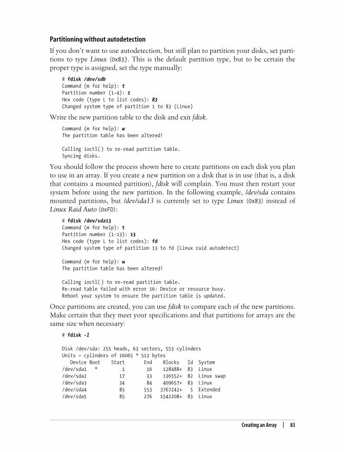
This is the Title of the Book, eMatter EditionCopyright © 2008 O’Reilly & Associates, Inc. All rights reserved.
Creating an Array | 83
Partitioning without autodetection
If you don’t want to use autodetection, but still plan to partition your disks, set parti-tions to type Linux (0x83). This is the default partition type, but to be certain theproper type is assigned, set the type manually:
# fdisk /dev/sdbCommand (m for help): tPartition number (1-4): 1Hex code (type L to list codes): 83Changed system type of partition 1 to 83 (Linux)
Write the new partition table to the disk and exit fdisk.
Command (m for help): wThe partition table has been altered!
Calling ioctl( ) to re-read partition table.Syncing disks.
You should follow the process shown here to create partitions on each disk you planto use in an array. If you create a new partition on a disk that is in use (that is, a diskthat contains a mounted partition), fdisk will complain. You must then restart yoursystem before using the new partition. In the following example, /dev/sda containsmounted partitions, but /dev/sda13 is currently set to type Linux (0x83) instead ofLinux Raid Auto (0xFD):
# fdisk /dev/sda13Command (m for help): tPartition number (1-13): 13Hex code (type L to list codes): fdChanged system type of partition 13 to fd (Linux raid autodetect)
Command (m for help): wThe partition table has been altered!
Calling ioctl( ) to re-read partition table.Re-read table failed with error 16: Device or resource busy.Reboot your system to ensure the partition table is updated.
Once partitions are created, you can use fdisk to compare each of the new partitions.Make certain that they meet your specifications and that partitions for arrays are thesame size when necessary:
# fdisk -l
Disk /dev/sda: 255 heads, 63 sectors, 553 cylindersUnits = cylinders of 16065 * 512 bytes Device Boot Start End Blocks Id System/dev/sda1 * 1 16 128488+ 83 Linux/dev/sda2 17 33 136552+ 82 Linux swap/dev/sda3 34 84 409657+ 83 Linux/dev/sda4 85 553 3767242+ 5 Extended/dev/sda5 85 276 1542208+ 83 Linux

This is the Title of the Book, eMatter EditionCopyright © 2008 O’Reilly & Associates, Inc. All rights reserved.
84 | Chapter 3: Getting Started: Building a Software RAID
/dev/sda6 277 407 1052226 83 Linux/dev/sda7 408 553 1172713+ 83 Linux
Disk /dev/sdb: 255 heads, 63 sectors, 1116 cylindersUnits = cylinders of 16065 * 512 bytes Device Boot Start End Blocks Id System/dev/sdb1 1 1116 8964238+ fd Linux raid autodetect
Disk /dev/sdc: 255 heads, 63 sectors, 1116 cylindersUnits = cylinders of 16065 * 512 bytes Device Boot Start End Blocks Id System/dev/sdc1 1 1116 8964238+ fd Linux raid autodetect
Disk /dev/sdd: 255 heads, 63 sectors, 1116 cylindersUnits = cylinders of 16065 * 512 bytes Device Boot Start End Blocks Id System
In addition to the system drive, two partitions are defined in the preceding listing.There is a partition on each of the second and third SCSI drives: /dev/sdb1 and /dev/sdc1. A fourth drive with no partitions defined resides at /dev/sdd.
Linear (Append) ModeLinear mode requires a minimum of two disks, but does not require that memberdisks be the same size or type. Since the system writes to each disk until it is full, thespeed and size of individual disks is largely irrelevant, in terms of aggregate RAIDperformance.
Important Rules for PartitioningHere are some points to remember when you are partitioning.
• If you don’t require autodetection and plan to use whole disks as array mem-bers, you don’t need to partition member disks individually.
• Set partitions to type Linux Raid Auto (0xFD) if you want the kernel to automati-cally start arrays at boot time. Otherwise, leave them as Linux (0x83).
• RAID-1 and RAID-4/5 arrays should contain member disks that have partitionsof the same size. If these arrays contain partitions of differing sizes, the largerpartitions will be truncated to reflect the size of the smallest partition.
• RAID-0 and linear mode arrays can contain partitions that have varying sizeswithout losing any disk space. Remember that when the smaller disks thatbelong to a RAID-0 become full, only the remaining disks are striped. So youmight see variable performance on a RAID-0 with member disks of differingsizes as the array fills up.
• Using matched drives is strongly recommended when working with any nonlin-ear mode array. Please see the “Matched Drives” section in Chapter 2 for fur-ther details.

This is the Title of the Book, eMatter EditionCopyright © 2008 O’Reilly & Associates, Inc. All rights reserved.
Creating an Array | 85
The following is a very simple linear array using /etc/raidtab:
# A linear array with two member disks
raiddev /dev/md0 raid-level linear chunk-size 64 persistent-superblock 1 nr-raid-disks 2
device /dev/sdb1 raid-disk 0
device /dev/sdc1 raid-disk 1
raiddev begins the definition of a new array, /dev/md0 in this case. All entries thatfollow apply to the previously defined array, until another raiddev entry is parsed.raid-level, as the name implies, sets the array type for the current array.
As I mentioned earlier, chunk-size would normally define the number of kilobytes towrite to each member disk for arrays that support disk striping. However, whenworking with linear mode arrays, the chunk-size defines the rounding factor. Eachcomponent disk is sized so that it is a multiple of the rounding factor. Because of theway the RAID superblock is placed on each array member, rounding factors of lessthan 64 KB are effectively equal to 64 KB.
The chunk-size, regardless of what type of array is used, must be defined as anypower of two. In fact, for the rest of this chapter, we’ll create arrays with a 64 KBchunk-size. You might notice some errors in the system boot messages and your logfiles, which warn about using a chunk-size with linear mode (or RAID-1). Thesewarnings arise from the inconsistencies between the kernel RAID driver and therequirements of raidtools for parsing /etc/raidtab. These warnings can be safelyignored.
persistent-superblock takes a Boolean value and controls whether a RAID super-block is written to member disks. The persistent-superblock should always beenabled when creating new arrays, but can be disabled for backward compatibility.
nr-raid-disks indicates that there are two disks in the array /dev/md0. Later in thefile, each disk is defined by identifying its device name and its order in the array,using the device/raid-disk pair. To use more than two disks, you need only addadditional device and raid-disk entries and increment the nr-raid-disks value.
Once /etc/raidtab is created, the mkraid program is used to build and activate thearray:
# mkraid /dev/md0handling MD device /dev/md0analyzing super-blockdisk 0: /dev/sdb1, 17920476kB, raid superblock at 17920384kBdisk 1: /dev/sdc1, 17920476kB, raid superblock at 17920384kB

This is the Title of the Book, eMatter EditionCopyright © 2008 O’Reilly & Associates, Inc. All rights reserved.
86 | Chapter 3: Getting Started: Building a Software RAID
The array was created successfully.
If you use mdadm, you don’t need a configuration file. The array we showed previ-ously can be created with the following command:
# mdadm -Cv -llinear -n2 /dev/md0 /dev/sd{b,c}1mdadm: array /dev/md0 started.
The options are simple.
-C, --createCreate a new array.
-v, --verboseBe more verbose.
-l, --raid-levelSelect the RAID level: linear, 0, 1, 4, or 5.
-n, --raid-disksSet the number of member disks in the array.
In addition to the options, mdadm takes a RAID device and a list of member parti-tions as its parameters. Note that the member disks are specified using standard shellexpansions. The disk letters encapsulated in braces are expanded into /dev/sdb1 and/dev/sdc1 when mdadm is run. Consult the manual pages for your shell as needed; Iuse bash.
Increasing the number of member disks using -n or --raid-devices allows you to spec-ify additional disks to be included in the array. List more disks on the command lineindividually, or as part of the glob (/dev/sd{b,c,d}1, for example). You could also usethe long form of the command to accomplish the same task.
# mdadm --create --verbose --level=linear --raid-devices=2 \/dev/md0 /dev/sdb1 /dev/sdc1
I’ll use the short form of the command through the rest of this chapter. Chapter 4contains a complete reference to all of the options in mdadm.
Both mkraid and mdadm automatically activate newly created arrays. Informationabout the array and its member disks is now available via the /proc/mdstat pseudo-file.
# cat /proc/mdstatPersonalities : [linear] [raid0] [raid1] [raid5]read_ahead 1024 sectorsmd0 : active linear sdc1[1] sdb1[0] 35840768 blocks 64k rounding
unused devices: <none>
Next, create a filesystem on the new array. In this example, and throughout the restof this chapter, I’ll use the ext2 filesystem. If you want to use another filesystem, then

This is the Title of the Book, eMatter EditionCopyright © 2008 O’Reilly & Associates, Inc. All rights reserved.
Creating an Array | 87
simply substitute that command in place of mke2fs. Chapter 6 covers some newerfilesystems available for Linux.
# mke2fs /dev/md0mke2fs 1.27 (8-Mar-2002)Filesystem label=OS type: LinuxBlock size=4096 (log=2)Fragment size=4096 (log=2)4480448 inodes, 8960192 blocks448009 blocks (5.00%) reserved for the super userFirst data block=0274 block groups32768 blocks per group, 32768 fragments per group16352 inodes per groupSuperblock backups stored on blocks: 32768, 98304, 163840, 229376, 294912, 819200, 884736, 1605632, 2654208, / 4096000, 7962624
Writing inode tables: doneWriting superblocks and filesystem accounting information: done
The preceding commands (mkraid or mdadm, and mke2fs) need to be executed onlyonce. Each time the system boots, mount the array like any normal hard disk parti-tion:
# mount /dev/md0 /mnt/raid/linear# df -h /mnt/raid/linearFilesystem Size Used Avail Use% Mounted on/dev/md0 34G 20k 31G 1% /mnt/raid/linear
You can modify your rc scripts to mount the array after it has been activated by usingraidstart or mdadm. If you are using RAID autodetection, then an entry for the arraycan also be added to /etc/fstab so it will be mounted automatically when the systemrestarts.
/dev/md0 /mnt/raid/linear ext2 defaults 1 2
Now, when the system restarts, the array (containing an ext2 filesystem) is mountedat /mnt/raid/linear and is usable like any normal filesystem. You can install software,store music, video, and image files, or create a database.
Be warned that some distributions (Red Hat, for one) halt system ini-tialization if an /etc/fstab entry could not be properly checked andmounted. So if the kernel doesn’t automatically start your array, anentry in /etc/fstab might be preventing the system from booting suc-cessfully. It’s a good idea to place commands that will manually startarrays in your initialization scripts before filesystems are checked andmounted, even if you’re already successfully using autodetection. Thiswill provide additional stability and, at worst, display some innocu-ous warnings on the console.

This is the Title of the Book, eMatter EditionCopyright © 2008 O’Reilly & Associates, Inc. All rights reserved.
88 | Chapter 3: Getting Started: Building a Software RAID
Linear mode is also good for reusing old ATA disks that vary in speed and sizebecause the variations between these disks will have minimal impact on the overallperformance of the array. The following example shows four ATA drives as mem-bers of a linear array:
# A linear array with four ATA member disks
raiddev /dev/md0 raid-level linear chunk-size 64 persistent-superblock 1 nr-raid-disks 4
device /dev/hda1 raid-disk 0
device /dev/hdb1 raid-disk 1
device /dev/hdc1 raid-disk 2
device /dev/hdd1 raid-disk 3
Use mdadm to create an identical array:
# mdadm -Cv -llinear -n4 /dev/md0 /dev/hd{a,b,c,d}1
RAID-0 (Striping)You can create a stripe with raidtools by making a few simple changes to the /etc/raidtab file used earlier for the linear mode array:
# A striped array with two member disks
raiddev /dev/md0raid-level 0 chunk-size 64 persistent-superblock 1 nr-raid-disks 2
device /dev/sdb1 raid-disk 0
device /dev/sdc1 raid-disk 1
Since you’ve changed the array type to striped (0), the chunk-size now has an impacton array performance. Since the chunk-size defines the amount of data that gets writ-ten to the member disk during each write, choosing a chunk-size that approximatesthe average write size (average file size) is desirable. Remember that unless you first

This is the Title of the Book, eMatter EditionCopyright © 2008 O’Reilly & Associates, Inc. All rights reserved.
Creating an Array | 89
erase the RAID superblocks from previously used disks, mdadm will prompt you forconfirmation.
Run mkraid to create and activate the RAID-0:
# mkraid /dev/md0handling MD device /dev/md0analyzing super-blockdisk 0: /dev/sdb1, 17920476kB, raid superblock at 17920384kBdisk 1: /dev/sdc1, 17920476kB, raid superblock at 17920384kB
Alternatively, use mdadm to create a two-disk stripe with a 64 KB chunk-size on /dev/md0, using disk partitions /dev/sdb1 and /dev/sdc1:
# mdadm -Cv -l0 -c64 -n2 /dev/md0 /dev/sd{b,c}1mdadm: array /dev/md0 started.
/proc/mdstat now reports that the new RAID-0 array has been created and is online:
# cat /proc/mdstatPersonalities : [linear] [raid0] [raid1] [raid5]read_ahead 1024 sectorsmd0 : active raid0 sdc1[1] sdb1[0] 35840768 blocks 64k chunks
You can now use mke2fs to create a filesystem:
unused devices: <none>
Separating disks in a RAID-0 onto different controllers will help improve your over-all array performance. You can arrange device/raid-disk entries in your /etc/raidtabfile contrary to the physical layout of disks and controllers. In this example, I havefour disks connected to a two-channel SCSI controller. /dev/sda and /dev/sdb are onchannel A, and /dev/sdc and /dev/sdd are on channel B. Notice how I alternate thedevice entries in this example /etc/raidtab file:
raiddev /dev/md0 raid-level 0 chunk-size 64 persistent-superblock 1 nr-raid-disks 4
device /dev/sda1 raid-disk 0
device /dev/sdc1 raid-disk 1
device /dev/sdb1 raid-disk 2
device /dev/sdd1 raid-disk 3

This is the Title of the Book, eMatter EditionCopyright © 2008 O’Reilly & Associates, Inc. All rights reserved.
90 | Chapter 3: Getting Started: Building a Software RAID
When using mdadm, simply alternate devices on the command line to achieve thesame effect:
# mdadm -Cv -l0 -n4 -c64 /dev/md0 /dev/sd{a,c,b,d}1
You can follow this methodology for any number of controllers. Remember thatLinux will logically arrange disks in detection order, beginning with /dev/sda.
RAID-1 (Mirroring)Setting up a mirror is slightly different from using linear mode or RAID-0. Wealready know that mirroring replicates data across all member disks. This allows aRAID-1 to continue functioning even if a disk fails. The simplest RAID-1 configura-tion must contain at least two member disks. In this example, /dev/sdb1 and /dev/sdc1 are member disks of the RAID-1 at /dev/md0:
# A RAID-1 with two member disks
raiddev /dev/md0 raid-level 1 nr-raid-disks 2 chunk-size 64
device /dev/sdb1 raid-disk 0
device /dev/sdc1 raid-disk 1
chunk-size has no effect on RAID-1 because no disk striping is involved. But chunk-size is still required as a placeholder. Note also that the persistent-superblock isn’tneeded for RAID-1. Use mkraid to create this array:
# mkraid /dev/md0
handling MD device /dev/md0analyzing super-blockdisk 0: /dev/sdb1, 17920476kB, raid superblock at 17920384kBdisk 1: /dev/sdc1, 17920476kB, raid superblock at 17920384kB
Or, using mdadm:
# mdadm -Cv -l1 -n2 /dev/md0 /dev/sd{b,c}1mdadm: array /dev/md0 started.
Whenever a new mirror is created, resynchronization occurs:
# cat /proc/mdstatPersonalities : [linear] [raid0] [raid1] [raid5]read_ahead 1024 sectorsmd0 : active raid1 sdc1[1] sdb1[0] 17920384 blocks [2/2] [UU] [= = = = = = = =>............] resync = 40.2% (7212864/17920384)finish=6.4min speed=27652K/secunused devices: <none>

This is the Title of the Book, eMatter EditionCopyright © 2008 O’Reilly & Associates, Inc. All rights reserved.
Creating an Array | 91
Now /proc/mdstat reports information about the array and also includes informationabout the resynchronization process. Resynchronization takes place whenever a newarray that supports data redundancy is initialized for the first time. The resynchroni-zation process ensures that all disks in a mirror contain exactly the same data.
The resynchronization is about 40 percent done and should be completed in lessthan six and a half minutes. You can begin creating a filesystem on the array evenbefore resynchronization completes, but you probably shouldn’t put the array intoproduction until it finishes.
Once the initial synchronization is complete, the progress bar no longer appears in/proc/mdstat:
# cat /proc/mdstatPersonalities : [linear] [raid0] [raid1] [raid5]read_ahead 1024 sectorsmd0 : active raid1 sdc1[1] sdb1[0] 17920384 blocks [2/2] [UU]
unused devices: <none>
When a disk does fail, it’s useful to be able to automatically promote another diskinto the array to replace the failed disk. When using raidtools, the nr-spare-disksand spare-disk parameters are used to define additional fault tolerance features. nr-spare-disks defines the number of extra, unused disks that the array can use toreplace failed disks. It’s also important to note that the sequence of spare disksbegins with zero and is not an offset of the nr-raid-disks variable. The spare-diskparameter is combined with the device parameter to define disks that will be insertedinto the array when a member disk fails. In this example, we still have a two-diskmirror consisting of /dev/sdb1 and /dev/sdc1. But this time, a spare disk (/dev/sdd1) isalso specified.
# A RAID-1 with 2 member disks and 1 spare disk
raiddev /dev/md0 raid-level 1 chunk-size 64 nr-raid-disks 2 nr-spare-disks 1
device /dev/sdb1 raid-disk 0
device /dev/sdc1 raid-disk 1
device /dev/sdd1 spare-disk 0

This is the Title of the Book, eMatter EditionCopyright © 2008 O’Reilly & Associates, Inc. All rights reserved.
92 | Chapter 3: Getting Started: Building a Software RAID
Create an array using this /etc/raidtab file with mkraid:
# mkraid /dev/md0handling MD device /dev/md0analyzing super-blockdisk 0: /dev/sdb1, 1614501kB, raid superblock at 1614400kBdisk 1: /dev/sdc1, 1614501kB, raid superblock at 1614400kBdisk 2: /dev/sdd1, 1614501kB, raid superblock at 1614400kB
If you are using mdadm, the -x flag defines the number of spare disks. Member disksare parsed from left to right on the command line. Thus, the first two disks listed inthis example (/dev/sdb1 and /dev/sdc1) become the active RAID members, and thelast disk (/dev/sdd1) becomes the spare disk.
# mdadm -Cv -l1 -n2 -x1 /dev/md0 /dev/sd{b,c,d}1mdadm: array /dev/md0 started.
If a disk in this array failed, the kernel would remove the failed drive (either /dev/sdb1 or /dev/sdc1) from /dev/md0, insert /dev/sdd1 into the array and start reconstruc-tion. In this case /dev/sdc1 has failed, as indicated by (F) in the following listing. Themd driver has automatically inserted spare disk /dev/sdd1 and begun recovery.
# cat /proc/mdstatPersonalities : [linear] [raid0] [raid1] [raid5]read_ahead 1024 sectorsmd0 : active raid1 sdd1[2] sdb1[1](F) sdb1[0] 17920384 blocks [2/1] [U_] [= = = =>................] recovery = 20.1% (3606592/17920384)finish=7.7min speed=30656K/secunused devices: <none>
RAID-1 is certainly not limited to arrays with only two member disks and one sparedisk. The following example describes a four-disk mirror with two dedicated sparedisks.
raiddev /dev/md0 raid-level 1 nr-raid-disks 4 nr-spare-disks 2 chunk-size 64
device /dev/sdb1 raid-disk 0
device /dev/sdc1 raid-disk 1
device /dev/sdd1 raid-disk 2
device /dev/sde1 raid-disk 3
device /dev/sdf1

This is the Title of the Book, eMatter EditionCopyright © 2008 O’Reilly & Associates, Inc. All rights reserved.
Creating an Array | 93
spare-disk 0
device /dev/sdg1 spare-disk 1
In this example, data is mirrored onto each raid-disk, so there are four copies of thedata, while the remaining two disks (/dev/sdf1 and /dev/sdg1) are spares that will beinserted automatically as members in the event of a disk failure.
mdadm users can replicate this setup with the following command:
# mdadm -Cv -l1 -n4 -x2 /dev/md0 /dev/sd{b,c,d,e,f,g}1
Failed disks and spare disks can also be manually removed from and inserted intoarrays as well. See the “Managing Disk Failures” section in Chapter 7 for more infor-mation on how to manage disk failures.
While this array can withstand multiple disk failures, it has a write overhead equal toits number of member disks. So each block of data is written to disk four times, mak-ing this arrangement very reliable, but extremely slow for write operations. Distribut-ing member disks across multiple controllers or I/O channels will help alleviate thewrite performance bottleneck. In contrast to the write performance hit, read perfor-mance is potentially fast because data can be read in parallel from all four members.A solution like this might be ideal for applications that are mission-critical and read-intensive, but that are generally read-only. Video-on-demand is a good example ofsuch a situation.
RAID-4 (Dedicated Parity)Since RAID-4 requires that a single drive be dedicated for storing parity information,a minimum of three drives are needed to make RAID-4 useful. Using less than threedrives would offer no increase in storage capacity over RAID-1.
A two-drive RAID-4 system would not offer better performance or fault tolerancewhen compared with RAID-1 or RAID-0. Therefore, in situations in which only twodrives are available, RAID-0 or RAID-1 should be used. Furthermore, RAID-5 offersmuch better performance when compared with RAID-4; almost everyone shouldchoose the former.
The following is a sample RAID-4 configuration using /etc/raidtab:
# RAID-4 with three member disks
raiddev /dev/md0 raid-level 4 chunk-size 64 persistent-superblock 1 nr-raid-disks 3
device /dev/sdb1 raid-disk 0

This is the Title of the Book, eMatter EditionCopyright © 2008 O’Reilly & Associates, Inc. All rights reserved.
94 | Chapter 3: Getting Started: Building a Software RAID
device /dev/sdc1 raid-disk 1
device /dev/sdd2 raid-disk 2
Use mkraid to construct this array:
# mkraid /dev/md0handling MD device /dev/md0analyzing super-blockdisk 0: /dev/sdb1, 17920476kB, raid superblock at 17920384kBdisk 1: /dev/sdc1, 17920476kB, raid superblock at 17920384kBdisk 2: /dev/sdd1, 17920476kB, raid superblock at 17920384kB
Or mdadm:
# mdadm -Cv -l4 -c64 -n3 /dev/md0 /dev/sd{b,c,d}1mdadm: array /dev/md0 started.
When this array is initialized, the last member disk listed in /etc/raidtab, or on thecommand line using mdadm, becomes the parity disk—/dev/sdd1, in this case. RAID-4 also supports spare disks.
Like other arrays with redundancy, /proc/mdstat will indicate that the initial resyn-chronization phase is underway. Parity RAID resynchronization ensures that allstripes contain the correct parity block.
# cat /proc/mdstatPersonalities : [linear] [raid0] [raid1] [raid5]read_ahead 1024 sectorsmd0 : active raid5 sdd1[2] sdc1[1] sdb1[0] 35840768 blocks level 4, 64k chunk, algorithm 0 [3/3] [UUU] [= = = = = = = =>............] resync = 40.2% (7206268/17920384) finish=8.1minspeed=21892K/secunused devices: <none>
As with RAID-1, you don’t have to wait until the initial resynchronization is com-plete before you create a filesystem. But remember that until the process is finished,you won’t have data redundancy. Notice that this time, the resynchronization isslower than with the RAID-1 we created earlier. That’s because parity informationmust be generated for each stripe. Also, RAID-4 has a write bottleneck caused by itsdedicated parity disk. You will also notice that resynchronization for a RAID-4requires a lot more CPU overhead. Examine the processes raid5d and raid5syncd,which handle the resynchronization, using top or another processes-monitoring pro-gram. On my test system, these processes use about 60 percent of the CPU duringthe resynchronization. That compares to about 2 percent for a RAID-1 initial syn-chronization.

This is the Title of the Book, eMatter EditionCopyright © 2008 O’Reilly & Associates, Inc. All rights reserved.
Creating an Array | 95
RAID-5 (Distributed Parity)RAID-5, for the same reasons as RAID-4, requires a minimum of three disks to bemore useful than a RAID-0 or RAID-1 array. Configuration is nearly identical toother levels, except for the addition of the parity-algorithm variable. parity-algorithm is used to select the algorithm that generates and checks the checksuminformation used to provide fault tolerance. A simple /etc/raidtab for RAID-5 isshown here:
# RAID-5 with three member disks
raiddev /dev/md0 raid-level 5 chunk-size 64 persistent-superblock 1 parity-algorithm left-symmetric nr-raid-disks 3
device /dev/sdb1 raid-disk 0
device /dev/sdc1 raid-disk 1
device /dev/sdd1 raid-disk 2
The left-symmetric algorithm will yield the best disk performance for a RAID-5,although this value can be changed to one of the other algorithms (right-symmetric,left-asymmetric, or right-asymmetric). While left-symmetric is the best choice, it isnot the default for raidtools, so be certain to explicitly specify it in /etc/raidtab. If youforget to include a parity-algorithm, then the array will default to left-asymmetric.
Execute mkraid to create this array:
# mkraid /dev/md0handling MD device /dev/md0analyzing super-blockdisk 0: /dev/sdb1, 17920476kB, raid superblock at 17920384kBdisk 1: /dev/sdc1, 17920476kB, raid superblock at 17920384kBdisk 2: /dev/sdd1, 17920476kB, raid superblock at 17920384kB
Create the same RAID-5 using mdadm:
# mdadm -Cv -l5 -c64 -n3 -pls /dev/md0 /dev/sd{b,c,d}1mdadm: array /dev/md0 started.
mdadm defaults to the left-symmetric algorithm, so you can safely omit the -poption from the command line.

This is the Title of the Book, eMatter EditionCopyright © 2008 O’Reilly & Associates, Inc. All rights reserved.
96 | Chapter 3: Getting Started: Building a Software RAID
After you issue mkraid or mdadm to create the array, /proc/mdstat will report infor-mation about the array, which, as in RAID-1 and RAID-4, must also undergo an ini-tial resynchronization:
# cat /proc/mdstatPersonalities : [linear] [raid0] [raid1] [raid5]read_ahead 1024 sectorsmd0 : active raid5 sdd1[2] sdc1[1] sdb1[0] 35840768 blocks level 5, 64k chunk, algorithm 2 [3/3] [UUU] [= = = = = = = =>............] resync = 40.2% (7219776/17920384)finish=6.0min speed=29329K/secunused devices: <none>
RAID-5 provides a cost-effective balance of performance and redundancy. You canadd more disks, using device/raid-disk, or spare disks, using device/spare-disk, tocreate large, fault-tolerant storage. The following example is for a five-disk RAID-5,with one spare disk. Notice once again how I’ve ordered the disks so they alternatebetween I/O channels.
# A 5-disk RAID-5 with one spare disk.
raiddev /dev/md0raid-level 5chunk-size 64persistent-superblock 1nr-raid-disks 5nr-spare-disks 1
device /dev/sdb1 raid-disk 0
device /dev/sdf1 raid-disk 1
device /dev/sdc1 raid-disk 2
device /dev/sdg1 raid-disk 3
device /dev/sdd1 raid-disk 4
# The spare disk. device /dev/sdh1 spare-disk 0
Or, create the same array using mdadm:
# mdadm -C -l5 -c64 -n5 -x1 /dev/md0 /dev/sd{b,f,c,g,d,h}1

This is the Title of the Book, eMatter EditionCopyright © 2008 O’Reilly & Associates, Inc. All rights reserved.
Creating an Array | 97
Hybrid ArraysOne of the most important features of software RAID is its ability to use existingarrays as member disks. This property allows you to not only create extremely largearrays, but to combine different RAID levels to achieve different degrees of perfor-mance and redundancy. The major benefit of using hybrid arrays is their ability towithstand multiple disk failures.
As I mentioned in Chapter 2, it’s advisable to spread member disks across multipleI/O channels whenever possible. This not only increases array performance but, inthe case of a mirror, also helps prevent array failure if an I/O channel becomesunavailable because of a disk controller failure or faulty cabling. For example, imag-ine that /dev/sda and /dev/sdb are member disks of /dev/md0, a RAID-1, and that theyare connected to the same controller A. If controller A fails, then all of /dev/md0becomes unavailable.
Now imagine that each disk is connected to its own controller. For instance, sup-pose /dev/sda is connected to controller A and /dev/sdb is connected to controller B.In this case, either controller A or B can fail without crashing /dev/md0 (seeFigure 3-5), because the other controller’s disk is still operational.
Figure 3-5. Using multiple controllers help prevent downtime.
Controller has failed, but Disk 1 onController A is still accessible.
RAID 1
Data
System bus
Disk controllerA
Disk controllerB
Disk 2/dev/sdb
Data0Data1
. . .DataNDisk 1
/dev/sda
Data0Data1
. . .DataN

This is the Title of the Book, eMatter EditionCopyright © 2008 O’Reilly & Associates, Inc. All rights reserved.
98 | Chapter 3: Getting Started: Building a Software RAID
Dispersing disks among multiple controllers is equally important when working withhybrid arrays. For example, take the case of a RAID-10 (mirrors combined into astripe). Assume that we have two mirrors that each contain two member disks. /dev/md0 contains /dev/sda and /dev/sdb, and /dev/md1 contains /dev/sdc and /dev/sdd. Ifwe placed both /dev/sda and /dev/sdb on controller A and the remaining disks on con-troller B, a failure of either controller would crash /dev/md2, our RAID-0(Figure 3-6). Since a RAID-0 cannot withstand any disk failures, the entire RAID-10would also become unavailable.
But what if we arranged our mirrors so that /dev/sda and /dev/sdc were on controllerA and /dev/sdb and /dev/sdd were on controller B? (See Figure 3-7.) In this case, thefailure of a single controller would only place our mirrors into degraded mode, leav-ing /dev/md2 operational.
Remember, you don’t have to rearrange hardware to facilitate this arrangement. Justcreate an /etc/raidtab or mdadm command that reflects the physical layout of yourhardware.
Figure 3-6. If disks are not arranged intelligently, a controller failure will crash a RAID-10.
When a disk controller fails, the entireRAID 10 (/dev/md2) becomes inoperative.
Disk controllerA
Disk controllerB
RAID 0/dev/md2
RAID 1/dev/md0
RAID 1/dev/md1
Data0Data2
. . .DataNDisk 1
/dev/sda
Data0Data2
. . .DataNDisk 2
/dev/sdbDisk 1
/dev/sdc
Data1Data3
. . .DataN+1
Disk 2/dev/sdd
Data1Data3
. . .DataN+1
Mirror 1 Mirror 2

This is the Title of the Book, eMatter EditionCopyright © 2008 O’Reilly & Associates, Inc. All rights reserved.
Creating an Array | 99
RAID-10 (striped mirror)
Since /etc/raidtab is parsed in order, it is essential to define arrays from the bottomup. That is, arrays that are also component disks should appear before the array thatcontains them. For example, a simple /etc/raidtab that defines a RAID-10 (two mir-rors combined into a stripe) might look like this:
A RAID-10: Two 2-disk mirrors are combined into a RAID-0
# The first mirror
raiddev /dev/md0 raid-level 1 chunk-size 64 nr-raid-disks 2
device /dev/sdb1 raid-disk 0
device /dev/sdc1 raid-disk 1
# The second mirror
raiddev /dev/md1
Figure 3-7. Distributing disks means you can survive controller loss.
When a disk controller fails, the entireRAID 10 (/dev/md2) is still operational.
Disk controllerA
Disk controllerB
RAID 0/dev/md2
Data0Data2
. . .DataN
Mirror1/dev/sda
Data1Data3
. . .DataN+1Mirror2
/dev/sdcMirror1
/dev/sdb
Data0Data2
. . .DataN
Mirror2/dev/sdd
Data1Data3
. . .DataN+1
Disk1 Disk2

This is the Title of the Book, eMatter EditionCopyright © 2008 O’Reilly & Associates, Inc. All rights reserved.
100 | Chapter 3: Getting Started: Building a Software RAID
raid-level 1 chunk-size 64 nr-raid-disks 2
device /dev/sdd1 raid-disk 0
device /dev/sde1 raid-disk 1
# The mirrors (/dev/md0 and /dev/md1 are# combined into a RAID-0.
raiddev /dev/md2 raid-level 0 chunk-size 64 persistent-superblock 1 nr-raid-disks 2
device /dev/md0 raid-disk 0
device /dev/md1 raid-disk 1
Given the preceding file, run mkraid on both of the mirrors (/dev/md0 and /dev/md1)and finally on the stripe (/dev/md2). The same feat can be accomplished with the fol-lowing mdadm commands:
# mdadm -C -n2 -l1 /dev/md0 /dev/sd{b,c}1# mdadm -C -n2 -l1 /dev/md1 /dev/sd{d,e}1# mdadm -C -n2 -l0 -c64 /dev/md2 /dev/md{0,1}
After each RAID-1 is initialized using mkraid or mdadm, it will commence resynchro-nization. /proc/mdstat should report two-disk mirrors at /dev/md0 and /dev/md1 anda RAID-0 at /dev/md2, which consists of /dev/md0 and /dev/md1.
# cat /proc/mdstatPersonalities : [raid0] [raid1]read_ahead 1024 sectorsmd2 : active raid0 md1[1] md0[0] 35840640 blocks 64k chunks
md1 : active raid1 sde1[1] sdd1[0] 17920384 blocks [2/2] [UU]
md0 : active raid1 sdc1[1] sdb1[0] 17920384 blocks [2/2] [UU]
unused devices: <none>

This is the Title of the Book, eMatter EditionCopyright © 2008 O’Reilly & Associates, Inc. All rights reserved.
Creating an Array | 101
Once all three arrays are activated, simply build a filesystem on the stripe—/dev/md2,in this case—and then mount /dev/md2.
mke2fs /dev/md2mount /dev/md2 /mnt/array
You could also add a spare disk to each of the mirroring arrays to make the solutionmore robust. And you can combine more than two mirrors into a RAID-0:
A RAID-10: Three 2-disk mirrors are combined into a RAID-0
# Each mirror has its own spare disk
raiddev /dev/md0 raid-level 1 chunk-size 64 nr-raid-disks 2 nr-spare-disks 1
device /dev/sdb1 raid-disk 0
device /dev/sdc1 raid-disk 1
device /dev/sdd1 spare-disk 0
# Mirror #2
raiddev /dev/md1 raid-level 1 chunk-size 64 nr-raid-disks 2 nr-spare-disks 1
device /dev/sde1 raid-disk 0
device /dev/sdf1 raid-disk 1
device /dev/sdg1 raid-disk 0
# Mirror #3
raiddev /dev/md2 raid-level 1 chunk-size 64 nr-raid-disks 2 nr-spare-disks 1
device /dev/sdh1

This is the Title of the Book, eMatter EditionCopyright © 2008 O’Reilly & Associates, Inc. All rights reserved.
102 | Chapter 3: Getting Started: Building a Software RAID
raid-disk 0
device /dev/sdi1 raid-disk 1
device /dev/sdj1 raid-disk 0
# Mirrors /dev/md0, /dev/md1 and /dev/md2 are# combined into a RAID-0, /dev/md3.
raiddev /dev/md3 raid-level 0 chunk-size 64 persistent-superblock 1 nr-raid-disks 3
device /dev/md0 raid-disk 0
device /dev/md1 raid-disk 1
device /dev/md2 raid-disk 2
Given the preceding file, run mkraid on each component RAID-1 and finally on /dev/md3, the RAID-0. Or, with mdadm:
# mdadm -C -n2 -l1 -x1 /dev/md0 /dev/sd{b,c,d}1# mdadm -C -n2 -l1 -x1 /dev/md1 /dev/sd{e,f,g}1# mdadm -C -n2 -l1 -x1 /dev/md1 /dev/sd{h,i,j}1# mdadm -C -n3 -l0 -c64 /dev/md2 /dev/md{0,1,2}
Clearly, it’s a waste of resources to provide a separate spare disk to each componentarray. Unfortunately, the md driver does not directly support the sharing of sparedisks. However, mdadm does let you share spare disks virtually. (See Chapters 4 and7.)
While RAID-10 is both fast and reliable, the wasted disk space can make it undesir-able. Half of all disk space on a RAID-10 is unusable.
RAID-50 (striped parity)
Since the disk requirements for RAID-10 are so high, you might find it more eco-nomical to combine RAID-5 into a RAID-0, a hybrid configuration called RAID-50.This hybrid array offers good read and write performance and can survive multipledisk failures, in the same manner that RAID-10 can. RAID-50 uses only one disk’sworth of space for each RAID-5 component array, making it more cost-effective. Thefollowing /etc/raidtab file defines two RAID-5 arrays, each consisting of three disks at/dev/md0 and /dev/md1. Those arrays are combined in a RAID-0 at /dev/md2.

This is the Title of the Book, eMatter EditionCopyright © 2008 O’Reilly & Associates, Inc. All rights reserved.
Creating an Array | 103
# First RAID-5
raiddev /dev/md0 raid-level 5 chunk-size 64 persistent-superblock 1 nr-raid-disks 3 parity-algorithm left-symmetric
device /dev/sdb1 raid-disk 0
device /dev/sdc1 raid-disk 1
device /dev/sdd1 raid-disk 2
# Second RAID-5
raiddev /dev/md1 raid-level 5 chunk-size 64 persistent-superblock 1 nr-raid-disks 3 parity-algorithm left-symmetric
device /dev/sde1 raid-disk 0
device /dev/sdf1 raid-disk 1
device /dev/sdg1 raid-disk 3
# The two RAID-5's are combined into a single# RAID-0.
raiddev /dev/md2 raid-level 0 chunk-size 64 persistent-superblock 1 nr-raid-disks 2
device /dev/md0 raid-disk 0
device /dev/md1 raid-disk 1

This is the Title of the Book, eMatter EditionCopyright © 2008 O’Reilly & Associates, Inc. All rights reserved.
104 | Chapter 3: Getting Started: Building a Software RAID
Use the following commands to create the same RAID-50 using mdadm:
# mdadm -C -n3 -l5 -c64 -pls /dev/md0 /dev/sd{b,c,d}1# mdadm -C -n3 -l5 -c64 -pls /dev/md1 /dev/sd{e,f,g}1# mdadm -C -n3 -l0 -c64 /dev/md2 /dev/md{0,1}
Since each RAID-5 must undergo its initial synchronization, the CPU will be heavilyutilized when you create a RAID-50. If the system is performing other tasks, then youmight want to wait until each initial synchronization has completed before creating afilesystem on /dev/md2 and carrying out any other administrative tasks. It might alsobe worthwhile to initialize each RAID-5 individually, waiting for its initial synchroni-zation to complete before creating the second one.
Finishing TouchesIf you use mdadm to create arrays, then you should probably take a minute to createan /etc/mdadm.conf file before you move on. First, create the file /etc/mdadm.conf,using any editor and a DEVICE line that lists all RAID member disks. On my system,for example, I create the file with the following line:
DEVICE /dev/sd*
This means that mdadm will examine all the sd device files on my system (/dev/sdb1through /dev/sdh1) when looking for member disks. Next, you should executemdadm with the --detail and --scan options to generate array lines and redirect theoutput so that it is appended to /etc/mdadm.conf.
# mdadm --detail --scan >> /etc/mdadm.conf
You should be left with an mdadm.conf file that contains the DEVICE line you created,plus an ARRAY line for each active RAID.
# cat /etc/mdadm.confDEVICE /dev/sd{b,c,d,e,f,g,h}1ARRAY /dev/md1 level=raid0 num-devices=5 \ UUID=66b78871:dc09da58:60f57124:978e5dbfARRAY /dev/md0 level=raid1 num-devices=2 \ UUID=b047f5a4:b6f459e0:fb04a323:46a1a012
Arrays that are not active will not be scanned by mdadm. Remember that you aren’tobligated to create an mdadm.conf file, but it will make managing arrays usingmdadm much easier. Now you can start both arrays with a simple command:
# mdadm -Asmdadm: /dev/md1 has been started with 5 drives.mdadm: /dev/md0 has been started with 2 drives.
Without the configuration file, you would need to know at least which disks weremembers. And you would need to execute a command such as the following for eacharray, every time you wanted to activate it:
# mdadm -A /dev/md1 /dev/sdc1 /dev/sdg1 /dev/sdd1 \ /dev/sdh1 /dev/sde1

This is the Title of the Book, eMatter EditionCopyright © 2008 O’Reilly & Associates, Inc. All rights reserved.
The Next Step | 105
If you’re using raidtools, start arrays with the raidstart command:
# raidstart /dev/md1
Or, start all arrays listed in /etc/raidtab:
# raidstart -a
As I mentioned earlier in this chapter, you can stop an active array by using eitherraidstop or mdadm -S. Don’t forget to unmount filesystems first.
# raidstop /dev/md0# mdadm -S /dev/md1
Irrespective of which management tools you decided to use, you can now add entriesfor your arrays to /etc/fstab, provided that you are using kernel RAID autodetection.Otherwise, you will need to add entries to your system startup scripts to activatearrays using mdadm or raidstart.
The Next StepEven if you spend large amounts of time planning and architecting your array, mak-ing a mistake is nearly inevitable. I think the best advice I can give for building thesesystems is: don’t worry if it doesn’t work perfectly the first time around. Trying outmultiple solutions and then deciding which one best suits your needs is much moreworthwhile than sitting at a whiteboard for three weeks, trying to plan in advance.Hopefully, this chapter has given you the information you need to get started inbuilding a software RAID solution.
Choosing an appropriate RAID level is only the first step. You might need to tradesome of the dollars you had planned to spend on storage capacity for a hardwarecontroller. Chapter 5 offers advice on how to make that decision. But software RAIDmight help you to prototype the right system without spending much money. Thenext chapter offers reference material on the md driver, raidtools, and mdadm, whichwill help supplement the material in this chapter. Chapter 4 also contains more /etc/raidtab and mdadm examples that can help make your configurations more robust byusing spare disks and hybrid arrays.

This is the Title of the Book, eMatter EditionCopyright © 2008 O’Reilly & Associates, Inc. All rights reserved.
106
Chapter 4tldp.orCHAPTER 4
Software RAIDReference
This chapter contains reference information about kernel RAID parameters andmanagement tools, including the raidtools package and the newer mdadm. It alsocontains many example configurations and an in-depth guide to software RAID andthe /proc filesystem.
Much of the material in this chapter is an amalgamation of my own experimentationwith software RAID, combined with material from manual pages, the Linux kernelsource code, and the various versions of the Software-RAID HOWTO and support-ing documents. Linas Vepstas wrote the original version of “The Software-RAIDHOWTO,” which was extremely useful to me when I built my first software RAID.A replacement document, written from the ground up, was released by Jakob Oester-gaard in January 2000.
The HOWTO documents, quick-starts, and examples that are distributed with theraidtools package and with many versions of Linux often contain erroneous or miss-ing information simply because they are out of date. While I am quick to complainabout some existing documentation, I am grateful to all the unpaid volunteers whohave, over the years, contributed to various parts of the RAID documentation, thekernel driver documentation, and the Linux-raid mailing list, especially JakobOestergard, Linas Vepstas, Neil Brown, and Ingo Molnar.
Kernel OptionsWhen you are configuring the kernel, the software RAID kernel features are all foundunder the Multiple devices driver support (RAID and LVM) subsection, regardless ofthe configuration method you use. Feel free to compile each level into the kernel stat-ically or as a module.
[*] Multiple devices driver support (RAID and LVM)<*> RAID support<M> Linear (append) mode<*> RAID-0 (striping) mode

This is the Title of the Book, eMatter EditionCopyright © 2008 O’Reilly & Associates, Inc. All rights reserved.
Kernel Options | 107
<M> RAID-1 (mirroring) mode<*> RAID-4/RAID-5 mode<M> Multipath I/O support
With older versions of the kernel, it was necessary to enable support for Develop-ment and/or Incomplete Code/Drivers. But with version 2.4, you no longer need toenable that option because the RAID code is stable and included as part of the stan-dard kernel.
Here is a list of kernel options for software RAID.
Multiple devices driver support (CONFIG_MD)CONFIG_MD enables support for representing multiple physical block devices as asingle logical device. CONFIG_MD must be enabled before RAID options will appearduring kernel configuration. CONFIG_MD is also needed for LVM support.
RAID support (CONFIG_BLK_DEV_MD)CONFIG_BLK_DEV_MD activates the base RAID driver, which contains code that isshared among all software RAID levels. Individual RAID levels must be selectedafter CONFIG_BLK_DEV_MD is enabled. RAID levels will not appear during kernelconfiguration unless this option is selected first.
Linear (append) mode (CONFIG_MD_LINEAR)CONFIG_MD_LINEAR allows multiple drives to be concatenated end-to-end so thatwhen a single member disk becomes full, data will be written to the next diskuntil all disks are full.
RAID-0 (striping) mode (CONFIG_MD_RAID0)CONFIG_MD_RAID0 enables support for RAID-0 (striping), which allows multipledisks to be arranged so they are evenly filled, one chunk at a time. If disks of dif-fering sizes are used, data is evenly distributed across all disks until one diskbecomes full. The data then continues to be evenly distributed across remainingdisks, although you won’t experience the same level of performance. Thus, ifthree 4 GB drives and a single 6 GB drive are used, data is evenly distributedacross all disks until the 4 GB drives (16 GB of data) are full. At that point, datais written only to the remaining 6 GB disk.
RAID-1 (mirroring) mode (CONFIG_MD_RAID1)CONFIG_MD_RAID1 activates support for disk mirroring. Each disk in a RAID-1 con-tains exactly the same data. There is an additional write operation for each disk,making write performance with RAID-1 slower than with other RAID levels.(Note that write performance is a function of the number of member disks.)However, read performance is improved because requests are distributed acrosseach disk in the mirror. If disks used in a RAID-1 are not the same size, each diskis truncated to the size of the smallest disk.
RAID-4/RAID-5 mode (CONFIG_MD_RAID5)CONFIG_MD_RAID5 enables RAID-4/RAID-5 mode and activates support for eitherof these parity RAID levels. The choice between the two is made in an /etc/

This is the Title of the Book, eMatter EditionCopyright © 2008 O’Reilly & Associates, Inc. All rights reserved.
108 | Chapter 4: Software RAID Reference
raidtab configuration file or on the command line with mdadm, and not in thekernel configuration itself. While RAID-4 stores parity information on a singledisk, RAID-5 provides redundancy by spreading parity information across eachmember disk. That means RAID-5 performs better than RAID-4 because opera-tions are distributed across all disks, instead of all but one disk. Like RAID-1,devices used in a RAID-4 or RAID-5 are truncated to the size of the smallestdisk.
Multipath I/O support (CONFIG_MD_MULTIPATH)CONFIG_MD_MULTIPATH enables support for multipath, which allows Linux toaddress a single disk using multiple controller paths. Disks that support multi-path operation are connected to more than one I/O channel. If one controller orchannel becomes unavailable, the operating system is still able to communicatewith the disk. Multipath is very new feature and is not covered in this book.
Deprecated Kernel OptionsThe following options are no longer shown in the configuration options for currentkernel revisions. These features were originally experimental, but are now a stan-dard part of the RAID subsystem. If you are using a kernel newer than 2.2.X, theoptions are enabled transparently as part of multiple devices support (CONFIG_BLK_DEV_MD). When using older kernels, you must explicitly enable these features if yourequire them.
Autodetect support (CONFIG_AUTODETECT_RAID)CONFIG_AUTODETECT_RAID enables support for RAID autodetection during boottime. Traditionally, users have to execute commands from their init scripts inorder to manually activate RAID devices. Autodetection allows the kernel toscan block devices for information about the arrays they belong to, and conse-quently to activate the devices while the system boots. This saves administratorsfrom having to run the raidstart command in the system’s startup files or at thecommand line. For RAID devices to be successfully autodetected, you must usefdisk or an equivalent partitioning program to set them to partition type LinuxRaid Auto (0xFD). Some programs might simply list Linux RAID as the partitiontype. Please refer to the “Partitioning with fdisk” section of Chapter 3 for moreinformation on this.
Boot support (CONFIG_MD_BOOT)CONFIG_MD_BOOT is available with the RAID patches for older kernels and is stan-dard in 2.4 and higher. Boot support allows arrays to be used at boot time,meaning that Linux can boot from a software RAID-1. That means a disk failurewon’t result in an unavailable system after a reboot. In addition to enabling thiskernel parameter, you need to pass special flags to the boot loader. You can finddetails on using LILO to boot an array in Chapter 7.

This is the Title of the Book, eMatter EditionCopyright © 2008 O’Reilly & Associates, Inc. All rights reserved.
/proc and Software RAID | 109
md Block Special FilesThe block special files /dev/md[0-255] provide access to software RAID devices. Themd driver uses a major number of 9. On most systems, all of these files are createdwhen the system is installed. If an md block special file is missing, you will get anerror like: error opening /dev/md31: No such file or directory from mdadm orraidtools. You can create the file yourself using the mknod command. The followingexample creates the block special file used to access /dev/md31 with a umask of 0660:
# mknod -m 0660 /dev/md31 b 9 31# chown root.disk /dev/md31
I specified b for block special file, 9 for the md major number, and 31 for the minornumber. In general, the minor number and the number for the device name are thesame. I also made certain that user and group ownership was set to root and disk,respectively. Repeat these commands for any device file you need to create manually.
Some distributions also come with the MAKEDEV program, usually found in /dev,although sometimes it is found as a symbolic link to /sbin/MAKEDEV. MAKEDEVcan be used to create all the special files for any character or block device. It’s moreuser-friendly than mknod, but MAKEDEV might not be available on all systems.
The following example uses MAKEDEV to create all the block special md files:
# /dev/MAKEDEV -v mdcreate md0 b 9 0 root:disk 660create md1 b 9 1 root:disk 660[...]create md30 b 9 30 root:disk 660create md31 b 9 31 root:disk 660
MAKEDEV will overwrite old device nodes. If you are working on a system on whichthe major or minor device numbers for your md devices have been altered, please becareful.
/proc and Software RAIDThe /proc filesystem is a virtual filesystem that provides information about the sys-tem and the running kernel. Files located in /proc provide vital information aboutmemory, devices, and processes. Here is also where you look for current informa-tion on active RAID devices. Virtual files under /proc provide information in realtime. By default, the kernel is configured to support the /proc filesystem. However, tobe certain that your kernel supports /proc, look for its entry in the File systems sub-section of the kernel configuration:
File systems ---> ... [*] /proc file system support ...

This is the Title of the Book, eMatter EditionCopyright © 2008 O’Reilly & Associates, Inc. All rights reserved.
110 | Chapter 4: Software RAID Reference
Files located in /proc are usually displayed using the cat command, but you can useany program in which you can view a text file. Most of the files in /proc merely pro-vide information (they are read-only), but some actually offer the means to manipu-late the way a running kernel operates. In that case, administrators usually write newvalues to a file using the echo command.
/proc/mdstat/proc/mdstat provides a way to examine the state of the md driver, including informa-tion about active software arrays. When no arrays are running, displaying /proc/mdstat simply shows which RAID levels the kernel supports.
# cat /proc/mdstatPersonalities : [linear] [raid0] [raid1] [raid5]read_ahead not setunused devices: <none>
In this example, there are no active arrays, but this kernel supports linear, RAID-0,RAID-1, and RAID-4/5. The read_ahead value is not currently set, because no arraysare active. read_ahead defines the number of sectors the kernel should cache duringsequential reads. Finally, unused devices is also empty, because there are no devicesin the md subsystem that are not currently in use by an array.
If arrays are defined, /proc/mdstat provides detailed information about them, asshown in the following code:
# cat /proc/mdstatPersonalities : [linear] [raid0] [raid1] [raid5]read_ahead 1024 sectorsmd2 : active raid1 sde1[1] sdd1[0] 17920384 blocks [2/2] [UU]
md1 : active raid0 sdc1[1] sdb1[0] 35840768 blocks 64k chunks
First, note that read_ahead is now set to 1024 sectors. That means that duringsequential reads, the kernel will attempt to cache a maximum of 1024 sectors worthof data, or about 512 K (1024 sectors, with approximately 512 bytes per sector). Thedefault value of 1024 sectors is a hard limit set by the md driver. Next, each array islisted, with the most recently activated array first. In this case, /dev/md2, a RAID-1, islisted first because it was activated most recently. Let’s examine /dev/md2 one line ata time to get a better understanding of the information reported:
md2 : active raid1 sde1[1] sdd1[0]
The first line is fairly straightforward. The array /dev/md2 is an active RAID-1 con-taining two member disks: /dev/sde1 and /dev/sdd1. The numbers in square brackets([ ]) following each member disk indicate the index number of that member disk.The information corresponds to either a raid-disk entry in /etc/raidtab or to the order

This is the Title of the Book, eMatter EditionCopyright © 2008 O’Reilly & Associates, Inc. All rights reserved.
/proc and Software RAID | 111
in which member disks were listed on the command line using mdadm. Here, /dev/sdd1 is the first raid-disk and /dev/sde1 is the second.
17920384 blocks [2/2] [UU]
This line shows information about the state of the array and its size. This array con-tains 17920384 blocks. Blocks reported in /proc/mdstat are always 1 KB in size. Thenext data element [2/2] shows that there are two disks in the array and that both areactive. The final field [UU] shows that both disks are error-free and operating nor-mally. If a disk had failed, these fields would indicate that disks were missing fromthe array and which disks had failed. For example:
17920384 blocks [2/1] [_U]
Notice that there are two member disks, but only one disk is currently operational([2/1]). The next field ([_U]) uses the underscore to indicate that the first disk hasfailed.
Depending on what type of array is defined, slightly different information is avail-able through /proc/mdstat.
md1 : active raid0 sdc1[1] sdb1[0] 35840768 blocks 64k chunks
This example describes a RAID-0 at /dev/md1. The first line provides the same infor-mation that the RAID-1 example provides, but the second line omits informationabout the status of member disks and instead includes information about the chunk-size. Since RAID-0 does not support redundancy, there’s no need to provide infor-mation about how many member disks are online versus how many have failed. Thefailure of a single disk in a RAID-0 means that the entire array is failed. chunk-size,which isn’t a factor when working with RAID-1, is a requirement for RAID-0. Sochunk-size information, instead of failure information, is provided for RAID-0arrays.
RAID-4 and RAID-5 arrays show a combination of the information provided forRAID-0 or RAID-1 arrays:
md1 : active raid5 sde1[3] sdd1[2] sdc1[1] sdb1[0] 53761152 blocks level 5, 64k chunk, algorithm 2 [4/4] [UUUU]
Here, a RAID-5 array defined at /dev/md1 contains four member disks. The secondline provides information about the chunk size and health of the array (four out offour disks are operational). In addition, the output shows the parity algorithm used,which is algorithm 2 in this case, corresponding to the left-symmetric algorithm. Thenumeric value reported here comes from a case switch found in the kernel RAID-5code in the file /usr/src/linux/drivers/block/raid5.c. Each of the usable algorithms isdefined there by name.
You might be wondering why the second line contains redundant information aboutwhich RAID level is in use. Let’s look at a RAID-4 example to clarify.

This is the Title of the Book, eMatter EditionCopyright © 2008 O’Reilly & Associates, Inc. All rights reserved.
112 | Chapter 4: Software RAID Reference
md1 : active raid5 sde1[3] sdd1[2] sdc1[1] sdb1[0] 53761152 blocks level 4, 64k chunk, algorithm 0 [4/4] [UUUU]
Notice that raid5 is listed as the array type on the first line, but level 4 is listed onthe second line. That’s because RAID-4 uses the RAID-5 driver. So when workingwith these RAID levels, be certain to examine the second line of md device output tomake certain that the proper RAID level is reported. Finally, while parity algorithm 0(left asymmetric) is listed, the parity algorithm has no effect on RAID-4. The entry issimply a placeholder and can be safely ignored.
Failed disks
When a disk fails, its status is reflected in /proc/mdstat.
md1 : active raid1 sdc1[1] sdb1[0](F) 17920384 blocks [2/1] [_U]
The first line lists disks in backward order, from most recently addedto first added. In this example, the (F) marker indicates that /dev/sdb1has failed. Note on the following line that there are two disks in thearray, but only one of them is active. The next element shows that thefirst disk (/dev/sdb1) is inactive and the second (/dev/sdc1) is in use. Soa U denotes a working disk, and an _ denotes a failed disk. The outputis a bit counterintuitive because the order of disks shown in the firstline is the opposite of the order of U or _ elements in the second line.Furthermore, the order in both lines can change as disks are added orremoved.
Resynchronization and reconstruction
/proc/mdstat also provides real-time information about array reconstruction andresynchronization. The following mirroring array is nearly halfway done with its ini-tial synchronization.
md1 : active raid1 sdc1[1] sdb1[0] 17920384 blocks [2/2] [UU] [= = = = = = = = =>...........] resync = 46.7% (8383640/17920384)finish=5.4min speed=29003K/sec
In this example, the process is 46.7 percent complete (also indicated by the progressbar). The first number in parentheses indicates how many blocks are ready, out ofthe total number of blocks (the second number). The resynchronization is expectedto take another 5.4 minutes, at the rate of roughly 29 MB (29003K) per second.
Recovery looks nearly identical, except that the failed disk and the newly inserteddisk are both displayed.
md1 : active raid1 sdd1[2] sdc1[1] sdb1[0](F) 17920384 blocks [2/1] [_U] [=>...................] recovery = 6.1% (1096408/17920384)finish=8.6min speed=32318K/sec

This is the Title of the Book, eMatter EditionCopyright © 2008 O’Reilly & Associates, Inc. All rights reserved.
/proc and Software RAID | 113
Note that on the third line, the process is called recovery. Remember from Chapter 3that recovery occurs when a new disk is inserted into an array after a disk fails.Resynchronization, on the other hand, happens when a new array is created or whendisks aren’t synchronized.
Although three disks are listed on the first output line, only two disks appear as arraymembers on the second line. That’s because, when this array was built, only twomember disks were defined. So the number of member disks will always remain con-stant. Each failed disk, like active member disks and spare disks, has its own diskindex. When a disk in the array fails, it is removed from the raid-disk index andadded to the failed-disk index, and that’s why the array disk count remains at two.
Once the recovery is complete, remove the old failed disk using raidhotremove ormdadm -r, and the /proc/mdstat entry will return to normal.
md1 : active raid1 sdd1[0] sdc1[1] 17920384 blocks [2/2] [UU]
If the spare disk also fails during recovery, the md driver will halt the reconstructionprocess and report both failures in /proc/mdstat, unless additional spare disks areavailable. In that case, the md driver will insert the next available spare disk andrestart the recovery process.
md0 : active raid5 sdh1[4](F) sdg1[3] sdd1[2] sdf1[1](F) sdb1[0] 53761152 blocks level 5, 64k chunk, algorithm 2 [4/3] [U_UU] resync=DELAYEDunused devices: <none>
/proc/sys/dev/raidThe /proc/sys directory provides interfaces for manipulating tunable kernel parame-ters. These parameters, which affect various aspects of the kernel, can be fine-tunedwhile the system is running. For more general information about /proc/sys, consultthe file in the /usr/src/linux/Documentation/sysctl directory of your kernel sourcecode, as well as /usr/src/linux/Documenation/filesystems/proc.txt.
Two files in the /proc/sys/dev/raid subdirectory provide a way to tune the speed atwhich array resynchronization (and reconstruction) takes place. speed_limit_min andspeed_limit_max define the minimum and maximum speeds at which resynchroniza-tion occur. The latter is especially useful on slower, or heavily utilized, systems,where you might find that the resynchronization process slows down the system toomuch. In that case, you could change the maximum speed—in effect, throttling theresynchronization process to a more suitable level. The md driver does provide itsown I/O thottling and will attempt to perform recovery nonintrusively, but usingspeed_limit_min and speed_limit_max can provide a quick fix if something goes hay-wire.

This is the Title of the Book, eMatter EditionCopyright © 2008 O’Reilly & Associates, Inc. All rights reserved.
114 | Chapter 4: Software RAID Reference
You’ll need to experiment with your system to see the maximum speed it can han-dle. Adjusting the minimum speed affects the low-end limit for resynchronization. Itmight be a good idea to simulate a drive failure and play with these values so thatyou aren’t surprised when a real disk failure happens.
You can simulate a disk failure by using the raidsetfaulty or mdadm --failcommands, which are described later in this chapter. You can also simu-late a disk failure by disconnecting the cable connected to a drive or byremoving a drive from a hot-swap enclosure. Remember, as I warnedin the section “Hot-swap” in Chapter 2, that you should not discon-nect hardware while the system is powered on, unless you have equip-ment that supports this operation. When simulating a disk failure, themd driver will not register that a disk has failed until an I/O operationis performed. That means you might have to access or create a file onthe array before the md driver reports the failure. Running the synccommand to flush filesystem buffers from memory to disk might alsobe required.
The default limits (100 KB and 100,000 KB, respectively) can be changed by echoingnew values into the pseudofiles:
# echo "5000" > /proc/sys/dev/raid/speed_limit_min# echo "50000" > /proc/sys/dev/raid/speed_limit_max
This changes the low and high limits to 5 MB and 50 MB, respectively. You can addthe above commands to your system initialization scripts if you want to change thedefault values of speed_limit_min and speed_limit_max automatically each time thesystem boots. Most distributions now provide the configuration file /etc/sysctl.conf topreserve changes to /proc/sys across reboots. For instance, you can alter resynchroni-zation speeds by adding the following lines to /etc/sysctl.conf:
dev.raid.speed_limit_min = 5000dev.raid.speed_limit_max = 50000
Consult the manual pages for sysctl and sysctl.conf for further details.
raidtoolsraidtools is the traditional package used to manage software arrays. Although thenewer mdadm is more feature-rich, raidtools is in wider use throughout the softwareRAID community. While it’s a bit more complex to manage arrays using raidtools,the package has proved reliable for many years. raidtools has remained at version 0.90 for several years, but the prerelease for version 1.0 of raidtools became availableduring the course of this writing, although it has not been officially released yet. Thenew version has some new utilities, including a tool that allows users to generate /etc/

This is the Title of the Book, eMatter EditionCopyright © 2008 O’Reilly & Associates, Inc. All rights reserved.
raidtools | 115
raidtab files by querying an active array, which is very useful if you’ve accidentallydeleted your /etc/raidtab file. The additions to version 1.0 are covered in this section,but keep in mind that I used a narrowly released beta version during my testing, andthat some functionality might have changed since then.
Version 1.0 fixes several known bugs in the 0.90 release of raidtools. raidtools-20010914 (version 0.90.0), in addition to having some minor bugs, was releasedwithout a vital utility, raidsetfaulty.This utility is used to manually induce a disk fail-ure and had been included with previous releases. Instead, raidtools-20010914shipped with a new program named raidhotgenerateerror, whose name makes it looklike a replacement for raidsetfaulty. Unfortunately, raidhotgenerateerror does notperform the same function as raidsetfaulty and should not be used as a replacement.raidhotgenerateerror is merely a utility for testing error handling in the md driver.This has caused some confusion among Linux RAID users. Because of these incon-sistencies, I advise against using raidtools-20010914. Instead, download and use theprevious release raidtools-19990824 from ftp.kernel.org/pub/daemons/raid/alpha. Ifyou are working with a version of raidtools that came installed with your distribu-tion, check to see if you have /sbin/raidsetfaulty on your system. If it doesn’t exist,then it’s likely that you are working with a repackaged version of raidtools-20010914. In that case, I recommend installing the previous version from source, orusing a newer version if one is available and tested. The beta version of raidtools-1.0corrects many of the problems with the raidtools-20010914 release and also containsraidsetfaulty. It likely that raidtools-1.0 will be in wide release by the time this bookis in print.
The /etc/raidtab FileThe current raidtools package requires a configuration file, which, by default, isnamed /etc/raidtab. The /etc/raidtab file contains a stanza about each software arrayconnected to the system. (A stanza is a collection of keywords and variables thatdescribe a single array.) The configuration is parsed from top to bottom so that pre-viously defined arrays may be used in subsequent stanzas. This is useful when creat-ing hybrid arrays like RAID-10, but it also means that the order of the stanzas in /etc/raidtab is extremely important. Each stanza begins with a raiddev directive and con-tinues with other directives from the following list.
raiddev mddeviceThe raiddev parameter begins the configuration of an array. All subsequentdirectives are assumed to refer to the most recent raiddev directive. raiddev takesthe full path to the device block special file as its argument (for example, raiddev/dev/md2). A unique raiddev directive is required for each array.

This is the Title of the Book, eMatter EditionCopyright © 2008 O’Reilly & Associates, Inc. All rights reserved.
116 | Chapter 4: Software RAID Reference
raid-level levelraid-level specifies the mode of the current array. This parameter takes analphanumeric value (see Table 4-1) that corresponds to kernel RAID levels.
Each raid-level directive defined in /etc/raidtab corresponds to the previouslydefined raiddev entry. In addition, support for the RAID level you have selectedusing raid-level must be compiled into your kernel, or be available as a load-able module, before the array can be started.
nr-raid-disks integerThe nr-raid-disks directive defines the number of active member disks in thecurrent array. This number does not include any spare disks that might be usedin an array that supports failover. (Use the nr-spare-disks parameter to indicatethe number of spare disks in the current array.) nr-raid-disks takes an integervalue greater than zero and is required once for each array that is defined usingthe raiddev parameter. Subsequently, a number of device and raid-disk entriesequal to the number defined with nr-raid-disks is required to specify the blockspecial file and disk order for each member disk.
nr-spare-disks integerSpare disks provide a mechanism for hot failover in the event of a drive failure.nr-spare-disks takes an integer value greater than zero and equal to the numberof available spares. As with nr-raid-disks, spares must be specified later byusing the device and spare-disk parameter. Spare disks are optional for arraysthat support failover (mirroring, RAID-4, and RAID-5). RAID-0 and linear modedo not support the use of spare disks, so nr-spare-disks is never used with theseRAID levels. Spares need to be defined in /etc/raidtab if you want automaticfailover. You can manually replace a failed disk using raidhotremove andraidhotadd, but that requires user intervention.
persistent-superblock booleanThe persistent-superblock directive determines whether an array contains aRAID superblock. The RAID superblock allocates a small area for metadata atthe end of each member disk. This metadata allows the kernel to identify disk
Table 4-1. raid-level parameters
raidtab entry Description
linear Linear concatenation
0 Striping
1 Mirroring
4 Single parity drive
5 Distributed parity
multipath Multipath I/O

This is the Title of the Book, eMatter EditionCopyright © 2008 O’Reilly & Associates, Inc. All rights reserved.
raidtools | 117
order and membership even in the event that a drive has moved to a differentcontroller. It is essential for autodetection. persistent-superblock should beenabled for any newly created array.
This parameter should be set to zero only when you need to provide backwardcompatibility with versions of the md driver that did not support a RAID super-block (version 0.35 and earlier). Set persistent-superblock to zero when a leg-acy array is being used with the new md driver.
parity-algorithm algorithm_nameThe parity-algorithm directive specifies the algorithm used to generate parityblocks. Note that this directive is used only with RAID-5. Parity is used to recon-struct data during a drive failure. There are four choices available, and theydetermine how parity is distributed throughout the array (Figure 4-1). Left-sym-metric, right-symmetric, left-asymmetric, and right-asymmetric are all validchoices, but left-symmetric is recommended because it yields the best overall per-formance.
Figure 4-1. Each algorithm distributes parity and data blocks differently.
/dev/md0
C
H
P2
M
R
P0
E
J
O
T
B
G
L
P3
Q
A
F
K
P
P4
D
P1
I
N
S
Data
/dev/sda1 /dev/sdb1 /dev/sdc1 /dev/sdd1 /dev/sde1
Left-symmetric /dev/md0
B
E
P2
P
S
D
G
J
M
P4
A
P1
L
O
R
P0
H
K
N
Q
C
F
I
P3
T
Data
/dev/sda1 /dev/sdb1 /dev/sdc1 /dev/sdd1 /dev/sde1
Right-symmetric
/dev/md0
C
G
P2
N
R
P0
H
L
P
T
B
F
J
P3
Q
A
E
I
M
P4
D
P1
K
O
S
Data
/dev/sda1 /dev/sdb1 /dev/sdc1 /dev/sdd1 /dev/sde1
Left-asymmetric /dev/md0
B
F
P2
O
S
D
H
L
P
P4
A
P1
J
N
R
P0
E
I
M
Q
C
G
K
P3
T
Data
/dev/sda1 /dev/sdb1 /dev/sdc1 /dev/sdd1 /dev/sde1
Right-asymmetric

This is the Title of the Book, eMatter EditionCopyright © 2008 O’Reilly & Associates, Inc. All rights reserved.
118 | Chapter 4: Software RAID Reference
You can specify the parity-algorithm by name in /etc/raidtab or use its numeri-cal equivalent (see Table 4-2). If you fail to specify a parity-algorithm in /etc/raidtab, the md driver will default to left-asymmetric, which is not an optimalchoice. So be certain to select left-symmetric explicitly.
chunk-size sizechunk-size specifies the size of the array stripe in kilobytes. Values may rangefrom 4 to 4096 kilobytes and must be powers of two. A bigger chunk-size willwork well for large, sequential operations, but a smaller chunk-size will yieldbetter performance for smaller, random operations. Most users should choose achunk-size of about 64 KB.
With linear mode, the chunk-size specifies the rounding factor for the array. Therounding factor helps evenly group I/O operations. It’s similar to the chunk-size,except it does not spread I/O across multiple disks.
chunk-size has no effect on RAID-1, but to satisfy error checking in raidtools,you must specify a valid chunk-size for any RAID-1 defined in /etc/raidtab.
The chunk-size is written into the RAID superblock during array ini-tialization. If you determine that you need to adjust the chunk-sizeafter your array is up and running, you will need to rebuild the arrayusing mkraid or mdadm. Be advised that your data will be lost if youneed to change the chunk-size for an array that has already beenbrought online. It is possible to adjust the chunk-size of an existingarray using raidreconf, but all the caveats regarding raidreconf stillapply. See the “raidreconf” reference entry later in this chapter.
device devpathThe device directive specifies the block special device of an individual arraymember. The full path to the block device should be used. The total number ofdevice entries must equal the sum of the numbers defined by nr-raid-disks andnr-spare-disks. In an array with four nr-raid-disks and one nr-spare-disk, atotal of five device entries are required. Each device entry must be paired witheither a raid-disk or a spare-disk index entry.
Table 4-2. Parity algorithms
Name Numeric value
left-asymmetric (default) 0
right-asymmetric 1
left-symmetric (best choice) 2
right-symmetric 3

This is the Title of the Book, eMatter EditionCopyright © 2008 O’Reilly & Associates, Inc. All rights reserved.
lsraid | 119
raid-disk indexraid-disk takes an integer value that indicates the sequence number of a mem-ber disk. The value of the raid-disk directive should increase sequentially foreach new device entry. After a new array is defined using raiddev, the indexnumber for all device entries is reset. That is to say, each array has a separate listof member disks starting at zero.
spare-disk indexThe spare-disk directive also takes an integer value beginning with zero. Thisparameter indicates the order of spare disks in an array. In the event of a diskfailure, available spare disks will be brought online in the order in which they areindexed in /etc/raidtab.
parity-disk indexparity-disk specifies an out-of-sequence member disk as the parity drive in aRAID-4 array. Normally, the last member disk is used for parity. However, theparity-disk directive allows administrators to flag any member disk as a paritydrive. This directive is accompanied by both a device entry and a raid-diskentry.
failed-disk indexThe failed-disk parameter lets you flag one or more member disks as failed dur-ing array initialization. Flagging a device as failed can be useful for testing dataredundancy without having to force a drive failure through a less gentle method.Flagging a device as failed also allows you to evaluate the performance of parityalgorithms. Finally, the parameter can be used to create an array with a missingdisk, which is a useful trick to use as part of migrating an existing system disk tosoftware RAID. (See “Converting to Software RAID” in Chapter 7 for moredetails.) failed-disk takes an integer value beginning with zero. Much like theparity-disk directive, failed-disk should be accompanied by device and raid-disk entries.
raidtools CommandsThe following referemce section describes the commands in the raidtools package.The fundamental command is mkraid command, which is responsible for creating aRAID device.
lsraidlsraid [mode] [options] -a mddevicelsraid [mode] [options] -d memberdevice
lsraid is included with release 1.0 of raidtools. It allows users to examine arrays andgenerate /etc/raidtab files by querying active arrays. lsraid is useful for checking devices,diagnosing problems, and recovering lost configuration files. lsraid was written by JoelBecker at Oracle Corporation.

This is the Title of the Book, eMatter EditionCopyright © 2008 O’Reilly & Associates, Inc. All rights reserved.
120 | Chapter 4: Software RAID Reference
Options
-ASpecifies array mode. Displays information about an array. When combined with the -aoption, array mode will query an active array. When combined with the -d option,array mode will read the RAID superblock from a member disk instead of querying thearray.
-DDenotes disk mode. Displays information about member disks. When used with the -aoption, disk mode returns information about each array member. When combinedwith -d, disk mode returns information about the specified member disks.
-RSpecifies raidtab mode. Queries an array or member disk and generates an /etc/raidtabfile based on the RAID superblock it finds.
-a deviceSelects an active md device to query. If the md device is inactive, lsraid indicates thedevice major and minor numbers and specifies that the array is offline.
-d deviceSelects which block device (member disk) to query. lsraid reads the RAID superblockfrom the member disk.
-fWhen combined with -A, displays only member disks that have failed.
-gWhen combined with -A, displays only member disks that are working.
-sWhen combined with -A, displays only spare disks in an array.
-lWhen combined with -D, displays the superblock from any member disk that may notbe consistent with the rest of the array.
-h, --helpDisplays configuration flags and exits.
-V, --versionDisplays the command version and exits.
Example usage
The following displays information about an md device:
# lsraid -A -a /dev/md0[dev 9, 0] /dev/md0 \ 226805E6.2D643610.E36B8421.BBD29055 online[dev 8, 17] /dev/sdb1 \ 226805E6.2D643610.E36B8421.BBD29055 good[dev 8, 33] /dev/sdc1 \ 226805E6.2D643610.E36B8421.BBD29055 good[dev 8, 49] /dev/sdd1 \ 226805E6.2D643610.E36B8421.BBD29055 good

This is the Title of the Book, eMatter EditionCopyright © 2008 O’Reilly & Associates, Inc. All rights reserved.
lsraid | 121
The following lists information about the array of which /dev/sdb1 is a member:
# lsraid -A -d /dev/sdb1[dev 9, 0] /dev/md0 \ 226805E6.2D643610.E36B8421.BBD29055 online[dev 8, 17] /dev/sdb1 \ 226805E6.2D643610.E36B8421.BBD29055 good[dev 8, 33] /dev/sdc1 \ 226805E6.2D643610.E36B8421.BBD29055 good[dev 8, 49] /dev/sdd1 \ 226805E6.2D643610.E36B8421.BBD29055 good
The following uses multiple instances of -a or -d to query more than one device at a time:
# lsraid -A -a /dev/md0 -a /dev/md1[dev 9, 0] /dev/md0 \ 226805E6.2D643610.E36B8421.BBD29055 online[dev 8, 17] /dev/sdb1 \ 226805E6.2D643610.E36B8421.BBD29055 good[dev 8, 33] /dev/sdc1 \ 226805E6.2D643610.E36B8421.BBD29055 good[dev 8, 49] /dev/sdd1 \ 226805E6.2D643610.E36B8421.BBD29055 good
[dev 9, 1] /dev/md1 \ F12F6203.49568B65.232305F6.08909BDA online[dev 8, 97] /dev/sdg1 \ F12F6203.49568B65.232305F6.08909BDA good[dev 8, 113] /dev/sdh1 \ F12F6203.49568B65.232305F6.08909BDA good
lsraid with the -R option is especially useful for generating an /etc/raidtab file that mighthave been lost because of file corruption or user error:
# lsraid -R -a /dev/md0# This raidtab was generated by lsraid version 0.3.0.# It was created from a query on the following devices:# /dev/md0
# md device [dev 9, 0] /dev/md0 queried onlineraiddev /dev/md0 raid-level 0 nr-raid-disks 3 nr-spare-disks 0 persistent-superblock 1 chunk-size 64
device /dev/sdb1 raid-disk 0 device /dev/sdc1 raid-disk 1 device /dev/sdd1 raid-disk 2
The previous example works only with an online array. If the array is offline, you cancombine the -R and -d options to generate an /etc/raidtab based on the RAID superblocks

This is the Title of the Book, eMatter EditionCopyright © 2008 O’Reilly & Associates, Inc. All rights reserved.
122 | Chapter 4: Software RAID Reference
found on individual disks. lsraid will attempt to collate member disks so you can usemultiple instances of -d to query all potential member disks, letting lsraid sort out the messfor you.
# lsraid -R -d /dev/sdb1 -d /dev/sdc1 -d /dev/sdd1 -d /dev/sde1 -d /dev/sdf1 -d /dev /sdg1 -d /dev/sdh1lsraid: Device "/dev/sde1" does not have a valid raid superblocklsraid: Device "/dev/sdf1" does not have a valid raid superblock# This raidtab was generated by lsraid version 0.3.0.# It was created from a query on the following devices:# /dev/sdb1# /dev/sdc1# /dev/sdd1# /dev/sde1# /dev/sdf1# /dev/sdg1# /dev/sdh1
# md device [dev 9, 0] /dev/md0 queried onlineraiddev /dev/md0 raid-level 0 nr-raid-disks 3 nr-spare-disks 0 persistent-superblock 1 chunk-size 64
device /dev/sdb1 raid-disk 0 device /dev/sdc1 raid-disk 1 device /dev/sdd1 raid-disk 2
# md device [dev 9, 1] /dev/md1 queried onlineraiddev /dev/md1 raid-level 1 nr-raid-disks 2 nr-spare-disks 0 persistent-superblock 1 chunk-size 64
device /dev/sdg1 raid-disk 0 device /dev/sdh1 raid-disk 1
Redirect the output of lsraid -R to create or append an /etc/raidtab file.

This is the Title of the Book, eMatter EditionCopyright © 2008 O’Reilly & Associates, Inc. All rights reserved.
mkraid | 123
mkraidmkraid [options] mddevice
mkraid (make raid) creates a RAID device from a set of block devices. All previous data onthe block devices will be lost, so be careful to back up any data on drives that you are plan-ning to include in an array. mkraid must be used to create arrays before filesystems are builtand requires an /etc/raidtab file for successful execution. See the “Example Usage” sectionbelow for details on the usage of mkraid.
Options
-c, --configfile filenameSpecifies the use of a configuration file other than the default /etc/raidtab.
-f, --force, --really-force, -RForces the initialization, even if data or filesystems are detected on any of the blockdevices to be included in the array. This is a fail-safe to prevent uninitiated users fromaccidentally destroying their data. The --really- force or -R flag is undocumented inthe command help and manual pages. When the -f or --force flags are used, mkraidwill display an additional warning and request that the command be retyped with the--really-force flag.
-h, --helpDisplays some helpful information about the command.
-u, --upgradeUpgrades an old RAID to the current version of the kernel’s RAID subsystem. Thisoption brings arrays with a RAID superblock up to the current md driver version. Itdoes not convert older arrays without superblocks. It is advisable to back up databefore attempting this operation.
-V, --versionDisplays the command’s version.
Example usage
The following creates an array at /dev/md0, as described in /etc/raidtab:
# mkraid /dev/md0
Using alternate configuration files is extremely useful if you are experimenting with manydifferent types of arrays. That way, you can keep copies of array configurations that havebeen successful, copying and combining them into /etc/raidtab when you’re ready to gointo production. The force flag is also useful when experimenting. The following creates,by force, the array /dev/md1 specified in the alternate configuration file /home/derek/myraidtab:
# mkraid --really-force -c /home/derek/myraidtab /dev/md1
The following upgrades an array to the kernel’s current version:
# raidstop /dev/md0# mkraid -u /dev/md0

This is the Title of the Book, eMatter EditionCopyright © 2008 O’Reilly & Associates, Inc. All rights reserved.
124 | Chapter 4: Software RAID Reference
raidhotaddraidhotadd mdevice memberdevice
raidhotadd inserts a new disk into a running array. After a failed drive has been removedusing raidhotadd, you can use this command to add a replacement drive.
When a new drive is introduced into an active array, reconstruction commences. There-fore, it’s a wise idea to add a new drive when you are certain that the recovery process willnot impact users. There may, of course, be times when waiting is not an option. You canalso fine-tune the speed at which recovery occurs in order to minimize the impact on thesystem. Refer to the “/proc/sys/dev/raid” section, earlier in this chapter, for details on howto throttle the recovery process.
Options
raidhotadd has no command-line options. It takes an md device and a member disk as itsonly arguments.
Example usage
The following adds /dev/sdc1 to the array /dev/md0:
# raidhotadd /dev/md0 /dev/sdc1
raidhotgenerateerrorraidhotgenerateerror mddevice memberdevice
raidhotgenerateerror should not be used to administer arrays. I mention it here onlybecause it has caused some confusion among Linux RAID users, as described near thebeginning of the “raidtools” section.
raidhotremoveraidhotremove mddevice memberdevice
raidhotremove removes a failed disk or a spare disk from an array. This is useful, in combi-nation with raidhotadd, for replacing a failed disk with a new, working disk. You could alsouse raidhotremove to remove a spare disk from an array so that it can be used in anotherarray, which is helpful when only one spare disk is available on a system with multiplearrays. In that case, you could use raidhotremove to pull the spare disk from a fully func-tional array and insert it into an array to make up for a failed disk.
There might be some instances when a disk is generating errors at the bus level, but hasn’tbeen marked as failed by the md driver. In that case, first use raidsetfaulty to fail the drivemanually, then use raidhotremove to pull it out of the array.
Options
raidhotremove has no command-line options. It takes an md device and a member disk asits only arguments.

This is the Title of the Book, eMatter EditionCopyright © 2008 O’Reilly & Associates, Inc. All rights reserved.
raidreconf | 125
Example usage
The following removes /dev/sdc1 from the array /dev/md0:
# raidhotremove /dev/md0 /dev/sdc1
raidhotremove and raidhotadd are merely software interfaces to theLinux kernel. They operate independently of any hardware connectedto the system. Using these commands does not mean you can safelydisconnect and reconnect drives from a powered-on system. Doingthis with hardware that does not support hot-swap could result in acomplete, unrecoverable system failure. For more information on hot-swap, consult the “Hot-swap” and “Single Connector Attachment(SCA)” sections in Chapter 2 and the “Managing Disk Failures” sec-tion in Chapter 7.
raidreconfraidreconf [options] -m mddevice
raidreconf can reconfigure certain properties of a RAID-0 or RAID-5 without data loss.
First, it can be used to resize an existing array. Normally, if you wanted to add or remove adisk from an array, you would need to back up your data, create a new array, and thenrestore the data. raidreconf circumvents the backup and restore steps by inserting orremoving a device and reorganizing the data so that it spans the remaining disks.
raidreconf can also be used to import or export data to or from an array. That means youcan take a single block device and use raidreconf to transfer data block-by-block onto analready existing software RAID. You can also export data from an existing array onto asingle block device, provided the target device has enough space. raidreconf can alsoconvert between RAID-0 and RAID-5. Finally, raidreconf can alter the chunk-size of anarray.
raidreconf does not support linear mode, RAID-1, or RAID-4 and should never be usedwith these RAID levels.
raidreconf was originally written by Jakob OEstergaard (he is also its current maintainer),but some critical bug fixes were implemented by Danny Cox. raidreconf is included withraidtools-1.0 and is also available from http://unthought.net/raidreconf/.
Be advised that raidreconf is still very much beta software, even though it looks like it couldbe widely distributed with raidtools in the near future. I strongly recommend checking itsweb site and version history for a list of known bugs. Take note of the following warningfrom http://unthought.net/raidreconf/:
Status is, that we do not currently know of any critical bugs in the software, it hasalready been used for both conversion and re-sizing of various arrays. However: it isvery likely that there are serious bugs that will destroy your data, possibly even ondisks not related directly to the array you are re-configuring.
raidreconf is also quite slow and requires that arrays be taken offline before any operationscan be performed, which means your data won’t be accessible for long periods of time. Onmy test system, for example, it took about three hours to add a disk to an existing five-disk

This is the Title of the Book, eMatter EditionCopyright © 2008 O’Reilly & Associates, Inc. All rights reserved.
126 | Chapter 4: Software RAID Reference
RAID-0 (using 18 GB drives). The time it takes to perform operations is directly related tothe size in blocks of the original array. For example, converting an existing two-disk RAID-0 to a six-disk RAID-5 took only 53 minutes on the same system, also using 18 GB drives.Despite all these caveats, raidreconf is still useful, simply because no alternative is avail-able. Just be certain to make a backup before using it on an array with data (as you shouldalways do when using beta software on critical data).
Options
-o raidtabSpecifies the raidtab file that contains the entry for the current (about to be reconfig-ured) array.
-n raidtabIndicates the raidtab file that contains the entry for the new (post-reconfigured) array.
-m mdevice, --mddev mddeviceSpecifies the array to reconfigure (for example, /dev/md0).
-i device, --import deviceImports data from a single block device into a new array.
-e device, --export deviceExports data from an existing array to a single block device.
-h, --helpDisplays some helpful information about the command.
-V, --versionDisplays the command’s version.
Example usage
The following example imports data from /dev/sda8 to a new array, /dev/md0, as defined in/etc/raidtab.
# raidreconf -i /dev/sda8 -n /etc/raidtab -m /dev/md0
Since /dev/sda8 and /dev/md0 differ in size, the filesystem that is already on /dev/sda8 willneed to be resized once it is copied to /dev/md0. Since it’s an ext2 filesystem, we can useresize2fs to change the size of the filesystem to fill the new array. But first, we have to fsckthe filesystem.
# e2fsck -fy /dev/md0# resize2fs /dev/md0
To resize an array, simply make a copy of your /etc/raidtab file and edit the stanza for thearray you want to resize to include a new disk, or to remove an existing one. Then useraidreconf. Remember that if you remove a disk, you need to be certain that the resultingarray is large enough to store the data that’s already on it. Whether you add a disk orremove one, you will need to resize the filesystem, using resize2fs or the appropriate utilityfor the filesystem you have chosen. If you add a disk, you should resize the filesystem afteryou run raidreconf. Shrink the filesystem before running raidreconf if you are removing adisk. In the next example, the array /dev/md0, defined in /etc/raidtab, will be converted tothe array defined in /root/raidtab.new:
# raidreconf -o /etc/raidtab -n /root/raidtab.new -m /dev/md0

This is the Title of the Book, eMatter EditionCopyright © 2008 O’Reilly & Associates, Inc. All rights reserved.
raidstart | 127
Once the conversion is completed, manually fsck the new array to ensure that everythingwas successful.
# e2fsck -f /dev/md0
If e2fsck (or another filesystem check program) returns no errors, raidreconf was a success.Errors mean that something went wrong and that you will need to restore from backups.Using e2fsck to repair any problems that are detected is likely to be a fruitless effort.
You can also change the raid-level in the new raidtab file to convert between RAID-0 andRAID-5. raidreconf also ships with a HOWTO written by Danny Cox.
raidsetfaultyraidsetfaulty mddevice memberdevice
Use raidsetfaulty to mark a member disk as failed. For example, if you suspect there areproblems with a disk, but the md driver hasn’t yet kicked it out of the array, you can useraidsetfaulty to fail the disk manually. Once a disk is failed, you can use raidhotremove topull it out of the array.
Options
raidsetfaulty has no command-line options. It takes an md device and a member disk as itsonly arguments.
Example usage
The following marks /dev/sdd1, a member of /dev/md0, as failed:
# raidsetfaulty /dev/md0 /dev/sdd1
Once raidsetfaulty is executed, /proc/mdstat will show that the disk has failed. If a sparedisk is available, recovery will automatically begin:
# cat /proc/mdstatPersonalities : [linear] [raid0] [raid1] [raid5] [multipath]read_ahead 1024 sectorsmd0 : active raid1 sdb1[2] sdd1[0](F) sdf1[1] 17920384 blocks [2/1] [_U] [>....................] recovery = 4.2% (764480/17920384)finish=10.4min speed=27302K/secunused devices: <none>
raidstartraidstart [options] mddevice
Although the modern kernel can now automatically detect and initialize RAID devices, itmight be necessary to manually start a device. Maybe the array was not properly initializedwhen the system booted, or perhaps you are simply experimenting with various types ofarrays. The command is also useful for restarting arrays in the unlikely event that they havecrashed.

This is the Title of the Book, eMatter EditionCopyright © 2008 O’Reilly & Associates, Inc. All rights reserved.
128 | Chapter 4: Software RAID Reference
Options
-a, --allApplies the command to all RAID devices found in /etc/raidtab. You will not need tospecify an mddevice.
-c, --configfile filenameUses a configuration file other than the default /etc/raidtab.
-h, --helpDisplays some helpful information about the command.
-V, --versionDisplays the command’s version.
Example usage
The following starts all arrays described in /etc/raidtab:
# raidstart -a
The following starts all arrays defined in /home/derek/example-raid0:
# raidstart -a -c /home/derek/example-raid0
The following starts only the array /dev/md2, as described in /etc/raidtab:
# raidstart /dev/md2
The following starts /dev/md2, as defined in /home/derek/example-raid0:
# raidstart -c /home/derek/example-raid0 /dev/md2
raidstart can also be included in system initialization scripts. This is quite useful in cases inwhich you don’t want the kernel to automatically detect and activate software arrays.Perhaps you would like to defer array startup until after some other scripts have run, ormaybe you are not using MS-DOS partitions and simply can’t autostart. Simply add theraidstart command to the appropriate system initialization files. Many distributions, infact, provide an initialization script that automatically parses /etc/raidtab and activatesarrays that it finds there. /etc/rc.d/rc.sysinit on Red Hat performs this function, for example.
I want to point out that many users report that raidstart is unreliable,especially in cases when the first component drive listed in /etc/raidtabhas failed or when major or minor numbers for component disks havechanged. For that reason, using kernel autodetection, or even mdadm,are recommended alternatives.
raidstopraidstop [options] mddevice
raidstop is the counterpart of raidstart and is useful for the same reasons. Since memberdisks can be allocated to only one array at a time, arrays must be deactivated by usingraidstop before their member disks can become available to use in new arrays.

This is the Title of the Book, eMatter EditionCopyright © 2008 O’Reilly & Associates, Inc. All rights reserved.
mdadm | 129
Options
-a, --allApplies command to all devices found in /etc/raidtab. You will not need to specify anmddevice.
-c, --configfile filenameSpecifies the use of a configuration file other than the default /etc/raidtab.
-h, --helpDisplays configuration flags and exits.
-V, --versionDisplays the command version and exit.
Example usage
The following stops all devices found in /etc/raidtab:
# raidstop -a
The following stops all arrays defined in /home/derek/example-raid0:
# raidstop -a -c /home/derek/example-raid0
The following stops /dev/md2, as defined in /home/derek/example-raid0:
# raidstart -c /home/derek/example-raid0 /dev/md2
The following stops only the array /dev/md2, as described in /etc/raidtab:
# raidstart /dev/md2
mdadmmdadm provides a convenient, single-command interface for managing softwarearrays under Linux. While mdadm is fully functional without the use of a configura-tion file, it does support a configuration file, /etc/mdadm.conf, which is more conciseand straightforward than /etc/raidtab. With mdadm, the configuration file is createdafter arrays, as a way to preserve information for arrays and member disks, so thatthey can be reactivated later. mdadm can be used as a total replacement for raidtools.
mdadmmdadm [mode] mddevice [options] memberdevices
mdadm has several modes of operation: Create, Build, Assemble, and Monitor. Each ofthese modes has its own command-line switch. In addition to these modes, there are manymanagement features that operate independently. These standalone features are groupedinto Manage or Miscellaneous mode. Most mdadm options have a long and a short form,although a few options have only a long form, to safeguard against using them acciden-tally. You can use whichever form you prefer.

This is the Title of the Book, eMatter EditionCopyright © 2008 O’Reilly & Associates, Inc. All rights reserved.
130 | Chapter 4: Software RAID Reference
General options for mdadm
-h, --helpDisplays general help for mdadm. The --help option can also be combined with otheroptions to display topic-specific help (for example, mdadm --create -help).
-V, --versionDisplays the mdadm version.
-v, --verboseIncreases verbosity. This option can be combined with other options to increase theamount of information that mdadm displays.
Create and Build modesmdadm --create mddevice [options] memberdevicesmdadm --build mddevice [options] memberdevices
The Create and Build modes are similar in that they are both used to create new arrays.However, Build mode is used only for backward compatibility, to create legacy arrayswithout a RAID superblock. Never use Build mode to create a new array.
Options
-C, --createCreates a new array.
-B, --buildCreates an old-style array without a RAID superblock.
-c, --chunk=Sets the array chunk-size in kilobytes. The chunk-size is a power of two between 4 and4096. For example, -c128 or --chunk=128 sets a chunk-size of 128 KB. The default is64 KB.
--rounding=Sets the rounding factor, which linear mode uses to align I/O operations. The roundingfactor is similar to chunk-size, with the exception that it does not distribute operationsacross multiple disks. The default value of 64 KB should be fine for most users. Thesame rules that apply to chunk-size apply to rounding (for example, --rounding=8 for 8KB rounding).
-l, --level=Specifies the RAID level: linear, RAID-0, RAID-1, RAID-4, or RAID-5. For Buildmode, only linear and RAID-0 are supported. For example, type -l5 or --level=5 forRAID-5.
-p, --parity=, --layout=Sets the parity algorithm for RAID-5. The parity algorithmoptions are left-asymmetric,right-asymmetric, left-symmetric, or right-symmetric. The best choice is left-symmetric(which is also the default). Choices may also be abbreviated as la, ra, ls, and rs. Exam-ples include -pls, --parity=left-symmetric, or --layout=left-symmetric.

This is the Title of the Book, eMatter EditionCopyright © 2008 O’Reilly & Associates, Inc. All rights reserved.
Create and Build modes | 131
-n, --raid-disks=Defines the number of member disks in an array. This is equivalent to nr-raid-diskswhen working with /etc/raidtab and raidtools. Like nr-raid-disks, it does not includespare disks. For example, type -n5 or --raid-disks=5 for five member disks.
-x, --spare-disks=Defines the number of spare disks in an array (equivalent to nr-spare-disks in /etc/raidtab). For example, enter -x1 or --spare-disks=1 for a single spare disk.
-z, --size=Manually sets the size in kilobytes of member disks in a RAID-1, RAID-4, or RAID-5.By default, the size is automatically computed by mdadm. The --size must be amultiple of the --chunk-size and must leave at least 128 KB at the end of each devicefor the RAID superblock. This is useful when working with disks of varying sizes. It’salso useful if the sizes of your disks are incorrectly calculated. For example, with achunk size of 64 KB, -z16000 or --size=16000 sets the size of each component disk to 1GB (64 KB * 16,000).
-f, --forceNormally when a RAID-5 is created, mdadm builds the array with a missing disk andthen inserts the remaining disk into the array. This induces recovery, instead of theslower resynchronization process. The --force option causes mdadm to create an arraythe traditional way, using resynchronization instead of recovery to initialize the array.
--runStarts the array even if mdadm detects problems. Using --run will prevent mdadm fromrequiring confirmation for potentially dangerous operations. For example, if mdadmdetects an existing filesystem or RAID superblock on a member disk, --run will none-theless force the array online, possibly destroying data.
--readonlyStarts the new array as read-only.
Example usage
All --create and --build operations must contain at least --raid-disks and --level options. Thefollowing creates a RAID-0 at /dev/md0 with a chunk-size of 128 KB and two memberdisks.
# mdadm --create /dev/md0 --level=0 --chunk=128 --raid-disks=2 /dev/sda1 /dev/sdb1
The following commands use the short form of mdadm to create a four-disk RAID-0 at /dev/md1. We don’t need to specify the chunk-size because the default chunk-size of 64 K iswhat we want.
# mdadm -C /dev/md1 -l0 -n4 /dev/sda1 /dev/sdb1 /dev/sdc1 /dev/sdd1
The list of component disks can be abbreviated using standard shell expansions. Consultthe manual pages for the particular shell you use to be sure you are using the propersemantics. I use the Bourne-again shell (bash).
# mdadm -C /dev/md1 -l0 -n4 /dev/sd[a-d]1# mdadm -C /dev/md1 -l0 -n4 -c64 /dev/sd{a,b,c,d}1
The three previous examples are equivalent. The list of devices is expanded from left toright, so /dev/sda1 becomes the first member disk in the array and /dev/sdd1 becomes thelast.

This is the Title of the Book, eMatter EditionCopyright © 2008 O’Reilly & Associates, Inc. All rights reserved.
132 | Chapter 4: Software RAID Reference
Linear mode uses a rounding factor instead of a chunk-size. This command creates a linearmode array with two disks and a rounding factor of 128 KB:
# mdadm -C /dev/md0 -llinear -n2 --rounding=128 /dev/hd{a,b}1
RAID-1 does not require a chunk-size:
# mdadm -C /dev/md0 -l1 -n2 /dev/sd{a,b}1
RAID-5 can take both both a chunk-size and a parity algorithm. The following examplecreates a five-disk RAID-5 at /dev/md0, using a chunk-size of 128 KB and the left-symmetricalgorithm:
# mdadm -C /dev/md0 -l5 -c128 -pls -n5 /dev/sd[a-e]1
By default, RAID-5 will automatically choose the left-symmetric parity algorithm, and alllevels that use striping default to a 64 KB chunk-size. So you don’t need to specify eitheroption on the command line if the defaults meet your needs.
Use the -x option to specify spare disks for arrays that support redundancy. In thisexample, a RAID-1 is created at /dev/md0 with /dev/sda1 and /dev/sdb1 as its member disks./dev/sde1 is a spare disk. The last disk listed on the command line becomes the spare disk.
# mdadm -C /dev/md0 -l1 -n2 -x1 /dev/sd{a,b,e}1
RAID-5 can also use spare disks. Normally, the last disk listed on the command linebecomes a spare disk (or the last two disks, if you specified -x2, and so on). However,because of the way that mdadm creates a RAID-5, this isn’t always the case. I mentioned inearlier chapters that resynchronization occurs when an array is initialized and that recoveryoccurs when an array rebuilds after being in degraded mode. Under RAID-5, recovery isfaster than resynchronization, so mdadm attempts to force recovery mode to synchronizedisks, rather than using the slower resynchronization process.
To facilitate this, mdadm creates an array with N-1 member disks and X+1 spare disks, asspecified by the --raid-disks (-n) and --spare-disks (-x) options. The kernel then initiatesrecovery when it notices the array is degraded and inserts one of the spare disks into thearray. In the following example, a five-disk RAID-5 with one spare disk is created at /dev/md0. /dev/sdf1 becomes the spare disk because mdadm assembles the array using the firstfour disks and then inserts the last (/dev/sdf1) of the two spare disks. This induces recovery,and /dev/sde1 becomes the only remaining spare disk.
# mdadm -C /dev/md0 -l5 -n5 -x1 /dev/sd{a,b,c,d,e,f}1
To force mdadm to initialize a RAID-5 using resynchronization instead of recovery, whilehonoring the device order at it appears on the command line, use the --force or -f option:
# mdadm -C /dev/md0 -f -l5 -n5 -x1 /dev/sd{a,b,c,d,e,f}1
mdadm can also create hybrid arrays:
# mdadm -C /dev/md0 -l1 -n2 -x1 /dev/sd{a,b,c}1# mdadm -C /dev/md1 -l1 -n2 -x1 /dev/sd{d,e,f}1# mdadm -C /dev/md2 -l0 -c64 -n2 /dev/md{0,1}
This example creates two mirroring arrays, each with a spare disk (/dev/md0 and /dev/md1).The third command combines both of these arrays into a RAID-0 with a chunk-size of 64KB.

This is the Title of the Book, eMatter EditionCopyright © 2008 O’Reilly & Associates, Inc. All rights reserved.
Assemble mode | 133
Assemble modemdadm --assemble mddevice [options] memberdevices
Assemble mode activates an array that has already been created using --create or --build. Itmight be helpful to think of Assemble mode as being similar to the raidstart command.
Options
-A, --assembleAssembles (starts) an existing array.
-u, --uuid=Specifies the UUID of an array to assemble. Disks are scanned for a RAID superblockcontaining the UUID and combined into an array.
-m, --super-minor=Uses the minor number to identify which member disks belong to an array. All soft-ware arrays have a major number of 9. By default, each array has a minor number thatcorresponds to the number of its device special name. Thus, /dev/md1 has a minornumber of 1, and /dev/md22 has a minor number of 22.
-s, --scanScans the configuration file /etc/mdadm.conf for information that could be used toassemble the array listed on the command line. This is useful for assembling arrayswithout having to remember their UUIDs, minor numbers, or component devices. Seethe “/etc/mdadm.conf” section, later in this chapter, for more information.
-c, --config=Specifies an alternate location for /etc/mdadm.conf. See the “/etc/mdadm.conf” section,later in this chapter, for more information.
-R, --runStarts an array when possible, even if some of its member disks are missing or unavail-able. This is useful for starting a RAID-1, RAID-4, or RAID-5 in degraded mode.
-f, --forceStarts an array even if the RAID superblocks found on member disks are inconsistent.
Example usage
Assemble the array named /dev/md1 from all disks whose names begin with /dev/sd andthat bear the specified UUID:
# mdadm --assemble /dev/md1 --uuid=0bd9fe83:702b6f5e:ab4d0e06:7dd7dbf4 /dev/sd*
You can examine the first partition of SCSI disks A through Z for the array with UUID0bd9fe83:702b6f5e:ab4d0e06:7dd7dbf4 and start it on /dev/md1:
# mdadm -A /dev/md1 -u0bd9fe83:702b6f5e:ab4d0e06:7dd7dbf4 /dev/sd[a-z]1

This is the Title of the Book, eMatter EditionCopyright © 2008 O’Reilly & Associates, Inc. All rights reserved.
134 | Chapter 4: Software RAID Reference
Search SCSI disks A through Z for member disks with the minor number 1 and combinethem into /dev/md1:
# mdadm -A /dev/md1 --super-minor=1 /dev/sd[a-z]1
The following command looks in /etc/mdadm.conf for a list of devices to scan for the minornumber 1 and the UUID 0bd9fe83:702b6f5e:ab4d0e06:7dd7dbf4. When both a UUID and aminor number are specified, both items must match the member disk for the disk to beconsidered an array component.
# mdadm -A /dev/md1 -m1 -u0bd9fe83:702b6f5e:ab4d0e06:7dd7dbf4
Combine the --scan option with the -A assemble option to activate an md device, using anarray entry found in /etc/mdadm.conf:
# mdadm -A --scan /dev/md0
Start all arrays that have entries in /etc/mdadm.conf:
# mdadm -As
Refer to the “/etc/mdadm.conf” section, later in this chapter, for further information on howto create a configuration file and use it with assemble mode.
Monitor modemdadm --monitor mddevice [options]
Monitor, or Follow, mode allows administrators to configure email notification, set upevent handling, and share spare disks between arrays.
Options
-F, --follow, --monitorEnables Follow mode for the specified array(s). mdadm will not exit when Followmode is invoked. Instead, it polls arrays and monitors for critical events. Run mdadmin the background as necessary.
-m, --mail=Sets the email address to notify when a failure event occurs. Example: -mderek or--mail=derek.
-p, --program=, --alert=Executes the specified program when an event occurs. You can create homegrownscripts to help mdadm monitor and manage arrays. Examples of these options include-pmymdmonitor.sh or --program=/usr/local/sbin/mymdmonitor.pl.
-d, --delay=Changes the number of seconds to wait between polling arrays (for example, -d30 or--delay=30 for thirty seconds). The default is one minute.
-s, --scanWhen used in Monitor mode, consults /etc/mdadm.conf for a MAILADDR line that indi-cates where to email results, and for a PROGRAM line that indicates what program to run,instead of taking those pieces of information from the command line.

This is the Title of the Book, eMatter EditionCopyright © 2008 O’Reilly & Associates, Inc. All rights reserved.
Monitor mode | 135
Example usage
When monitor mode is invoked, mdadm will not exit, so it’s a good idea to run it in thebackground and redirect its output to a file that you can examine. The following examplepolls /dev/md1 every sixty seconds (the default) and sends critical event notifications toroot:
# nohup mdadm --monitor /dev/md1 --mail=root &
If an md device is not specified on the command line, mdadm will monitor all devices listedin /etc/mdadm.conf. The next example monitors all arrays listed in the configuration andsends notifications to [email protected].
# nohup mdadm --monitor [email protected] &
It’s useful to invoke mdadm in monitor mode when the system boots. You can do this bycreating an rc script for it at specific runlevels or adding it to /etc/rc.local where available.Chapter 7 covers practical usage of mdadm --monitor.
mdadm reports the following events via email:
Fail mddeviceA member disk that was part of mddevice has failed and was marked as faulty.
FailSpare mddevice spare-diskThe spare-disk that was added to mddevice failed before reconstruction completed.
In addition to Fail and FailSpare, mdadm reports the following events to the program speci-fied on the command line using --program= or in /etc/mdadm.conf.
DeviceDisappeared mddeviceAn array that was active during the last poll is no longer active.
NewArray mddeviceAn array that was inactive during the last poll is now active.
RebuildStarted mddeviceThe array has begun reconstruction.
Rebuild[20,40,60,80] mddeviceThe percentage complete for an array that is undergoing resynchronization or recon-struction. The status is reported at 20, 40, 60, and 80 percent.
SpareActive mddevice spare-diskA spare disk that was inserted to replace a failed disk has been activated, meaning thatthe rebuild process has completed.
MoveSpare mddevice mddeviceA spare disk has been moved from one array to another.
Event names and device information is passed to the receiving program as command-lineoptions. So if you decide to develop your own monitoring utilities, parsing the commandline passed to your script or program will provide you with the event, the md device name,and in some cases, the name of a spare disk or additional md device. To get an idea of howthe events work, I suggest using echo as the program to execute:
# nohup mdadm --monitor --program=/bin/echo &

This is the Title of the Book, eMatter EditionCopyright © 2008 O’Reilly & Associates, Inc. All rights reserved.
136 | Chapter 4: Software RAID Reference
The previous example creates the file nohup.out in the current directory or in your homedirectory. Because we have set echo as the event program to execute, mdadm will print anyevent information to nohup.out.
The next example imports an email address and event program from /etc/mdadm.conf andpolls all arrays listed in the configuration file every thirty seconds:
# nohup mdadm --monitor --scan --delay=30 &
Manage and Miscellaneous modesmdadm [options] mddevice memberdevicesmdadm mddevice [options] memberdevicesmdadm [options] memberdevicesmdadm [options]
The remaining options fall into the loosely defined categories of Manage and Miscella-neous modes. For the most part, these options work individually, but some of them can becombined to provide additional functionality. Many of these options are used on arrays,while some of them are used directly on member disks. See the “Example usage” sectionthat follows for some common tasks.
Options
-Q, --queryQueries an array or member disk to determine array properties, member disk proper-ties, or both in cases when an array is also a member disk (in a hybrid array, forexample). --query displays very brief information: array size, RAID level, and status.For member disks, it displays the disk sequence instead of the array size.
-D, --detailPrints verbose details about an active array.
-E, --examinePrints the contents of the md superblock from a member disk. This is usually a singledevice, but in the case of hybrids, it can also be an array.
-b, --briefWhen combined with either --detail or -examine, generates a configuration file entryfor an array. When combined with --detail, an active array is queried and used togenerate the configuration entry. When combined with --examine, the RAID super-block is read from a member disk and used to generate the configuration entry. Ingeneral, it’s best to use the --detail form when possible because on-disk superblockscould occasionally contain incorrect information.
-s, --scanWhen combined with --detail or --examine, provides results similar to --brief. Thedifference in this case is that --scan queries multiple arrays or member disks and gener-ates /etc/mdadm.conf entries for each array it discovers. mdadm --detail --scan looks foractive arrays in /proc/mdstat and generates configuration file entries for each array.mdadm --examine --scan looks for a list of potential member disks in /etc/mdadm.conf,

This is the Title of the Book, eMatter EditionCopyright © 2008 O’Reilly & Associates, Inc. All rights reserved.
Manage and Miscellaneous modes | 137
reads the RAID superblock from each disk, and then generates a configuration line foreach unique array. See the “/etc/mdadm.conf” section, later in this chapter, for moreinformation.
-S, --stopStops a running array. Equivalent to the raidtools command raidstop.
-a, --addAdds a disk to an inactive array or hot-adds a disk to an active array. This optionworks like the raidtools command raidhotadd.
-r, --removeRemoves a member disk from an active array. This option works like the raidtoolscommand raidhotremove.
-f, --fail, --set-faultyMarks a member disk in an active array as failed. This option works like the raidtoolscommand raidsetfauly.
-R, --runStarts an inactive array. When mdadm assembles arrays that are missing componentdisks, it will mark the arrays as inactive, even if they can function with disks missing(for example, a RAID-1, RAID-4, or RAID-5 that is in degraded mode). The --runoption will start an inactive array that has already been assembled. --run works as astandalone option, but it can also be combined with --assemble to automatically start adegraded array.
-o, --readonlyMarks an array as read-only.
-w, --readwriteMarks an array as read/write.
--zero-superblockErases the RAID superblock from the specified device.
Example usage
The query option outputs brief information about an array or member disk. For example:
# mdadm --query /dev/md0:/dev/md0: 34.18GiB raid5 3 devices, 1 spare. Use mdadm --detail for more detail./dev/md0: No md super block found, not an md component.
When used on member disks, --query will output disk sequence information. Thefollowing example uses the short form of the command:
# mdadm -Q /dev/sdc1/dev/sdc1: is not an md array/dev/sdc1: device 2 in 3 device active raid5 md0. Use mdadm --examine for more detail.
When an array is also a member disk, as in the case of a hybrid array, --query displaysinformation about both of its roles:
# mdadm -Q /dev/md1/dev/md1: 17.09GiB raid1 2 devices, 0 spares. Use mdadm --detail for more detail./dev/md1: device 1 in 2 device active raid0 md2. Use mdadm --examine for more detail.

This is the Title of the Book, eMatter EditionCopyright © 2008 O’Reilly & Associates, Inc. All rights reserved.
138 | Chapter 4: Software RAID Reference
The output of mdadm --detail displays information about an active array. There is someoverlap between this information and the data found in /proc/mdstat, but mdadm providessome additional information. In the following example, we have a four-disk RAID-5:
# mdadm --detail /dev/md0/dev/md0: Version : 00.90.00 Creation Time : Wed Mar 13 06:52:41 2002 Raid Level : raid5 Array Size : 53761152 (51.27 GiB 55.05 GB) Device Size : 17920384 (17.09 GiB 18.35 GB) Raid Devices : 4 Total Devices : 4Preferred Minor : 0 Persistance : Superblock is persistant
Update Time : Wed Mar 13 06:52:41 2002 State : dirty, no-errors Active Devices : 4Working Devices : 4 Failed Devices : 0 Spare Devices : 0
Layout : left-symmetric Chunk Size : 64K
Number Major Minor RaidDisk State 0 8 17 0 active sync /dev/sdb1 1 8 33 1 active sync /dev/sdc1 2 8 49 2 active sync /dev/sdd1 3 8 65 3 active sync /dev/sde1 UUID : 3d793b9a:c1712878:1113a282:465e2c8f
The first section of the listing displays general information about the array, including theversion of the md driver that created it, the creation date and time, the RAID level, the totalsize, and the total number of disks.
The second section displays information about the current state of the array. Update Timereflects the last time that the array changed status. This includes disk failures, as well asnormal operations such as array activation. State reflects the health of the array; in thiscase, the array is operating within normal parameters, as indicated by no-errors. The dirtystate might be a bit confusing, since it implies that there is a problem. Dirty simply meansthat there are array stripes that haven’t yet been committed to disk by the kernel. When anarray is stopped, dirty stripes are written and the array becomes clean. Both dirty andclean indicate normal operation.
Next, a list of Active Devices, Working Devices, Failed Devices, and Spare Devices isdisplayed. Active Devices reflects the number of functioning (non-failed) array members,but does not include spare disks. Working Devices is the total number of non-failed disks inthe array (Active Devices + Spare Devices). Failed Devices and Spare Devices display thenumber of each of those types, respectively.

This is the Title of the Book, eMatter EditionCopyright © 2008 O’Reilly & Associates, Inc. All rights reserved.
Manage and Miscellaneous modes | 139
The next section displays properties that are specific to the RAID level. Layout reports theparity algorithm in use, followed by the Chunk Size in kilobytes. Because both of theseoptions are specific to various RAID levels, they will not appear in all output of mdadm -D.In this example, both settings are displayed because RAID-5 is in use. A mirroring arraywould display neither because it does not support striping and does not use parity, while aRAID-0 would display only Chunk Size.
The last section displays a list of all array member disks, including their major and minornumbers, their positions in the array, current states, and block special files. Finally, theUUID of the array, if available, is displayed.
The -E or --examine option is used to display information about a member disk, asopposed to information about the array.
# mdadm --examine /dev/sdb1/dev/sdb1: Magic : a92b4efc Version : 00.90.00 UUID : 3d793b9a:c1712878:1113a282:465e2c8f Creation Time : Wed Mar 13 06:52:41 2002 Raid Level : raid5 Device Size : 17920384 (17.09 GiB 18.35 GB) Raid Devices : 4 Total Devices : 4Preferred Minor : 0
Update Time : Wed Mar 13 06:52:41 2002 State : dirty, no-errors Active Devices : 4Working Devices : 4 Failed Devices : 0 Spare Devices : 0 Checksum : 79b87088 - correct Events : 0.1
Layout : left-symmetric Chunk Size : 64K
Number Major Minor RaidDisk Statethis 0 8 17 0 active sync /dev/sdb1 0 0 8 17 0 active sync /dev/sdb1 1 1 8 33 1 active sync /dev/sdc1 2 2 8 49 2 active sync /dev/sdd1 3 3 8 65 3 active sync /dev/sde1
The above output is from a member disk (/dev/sdb1) from the array used in the previous--detail example. The -E or --examine option reads the md superblock from an arraymember and displays the information found there. The --detail option, in contrast, looksat the array as a whole. --examine is used to query individual member disks. However,since you can combine arrays into larger arrays (such as RAID-10), the member disk thatis displayed by the --examine option could actually be an array in its own right, insteadof an individual disk. While much of the information provide by --detail and --examineoverlaps, you can see that there are some pieces of information that are unique to eachoption.

This is the Title of the Book, eMatter EditionCopyright © 2008 O’Reilly & Associates, Inc. All rights reserved.
140 | Chapter 4: Software RAID Reference
Magic shows the magic number* used by the kernel RAID subsystem to mark the beginningof a RAID superblock. This hexadecimal number (a92b4efc) is a constant defined in theLinux kernel. Every md superblock stores Checksum information about itself. When mdadmexamines a component disk, it computes the Checksum for the superblock and compares itto the value already stored there. In this case, that computation matched the value foundon the disk. If there had been a discrepancy, it would have been noted here. Immediatelyfollowing is the event counter, which displays the number of Events in the array’s history.
Combine the --brief option with --detail to generate array entries suitable for /etc/mdadm.conf. For instance, the following command generates an entry for /dev/md0. You might findit convenient to redirect the output to /etc/mdadm.conf/.
# mdadm --detail --brief /dev/md0ARRAY /dev/md0 level=raid5 num-devices=4 UUID=41d0ebc5:befadd9f:cfab6144:dfa13287
Stop the array at /dev/md0:
# mdadm --stop /dev/md0
Stop the arrays at /dev/md0, /dev/md1, and /dev/md2 using the short form of --stop:
# mdadm -S /dev/md0 /dev/md1 /dev/md2
Run an array that was partially assembled, but not activated, because a missing disk wouldhave started it in degraded mode:
# mdadm --run /dev/md0
Mark /dev/md0 as --readonly using the short form:
# mdadm -o /dev/md0.
Mark /dev/md0 as --readwrite using the short form:
# mdadm -w /dev/md0.
Erase the RAID superblock from /dev/sda1. This option has no short form.
# mdadm --zero-superblock /dev/sda1
The --zero-superblock option also works on multiple disks:
# mdadm --zero-superblock /dev/sd{a,b,c,d,e,f}1
/etc/mdadm.confAlthough mdadm does not rely on a configuration file, using one will make arraymanagement much easier. /etc/mdadm.conf contains four types of lines that provideinformation to mdadm. DEVICE lines tell mdadm which block devices are memberdisks of an array, and ARRAY helps mdadm identify arrays that have already been cre-ated. MAILADDR and PROGRAM lines provide information about where to send emailalerts and what program to execute when mdadm is monitoring arrays.
* Magic numbers have a few different definitions in computer programming. In this case, the magic numberis used to let programs like raidtools or mdadm know that a particular disk block marks the beginning of theRAID superblock. The number itself, in this case, is arbitrary and simply acts as a marker. See the magicnumber entry in the jargon file 4.3.1 for more information: http://www.tuxedo.org/jargon/html/entry/magic-number.html.

This is the Title of the Book, eMatter EditionCopyright © 2008 O’Reilly & Associates, Inc. All rights reserved.
Manage and Miscellaneous modes | 141
DEVICE lines
DEVICE entries have the following format:
DEVICE device1 device2 ... deviceN
DEVICE lines can contain a complete list of individual block devices or use shellexpansions to shorten the list and make managing the configuration file less tedious.In the following example, the first two ATA disks and all SCSI devices are consid-ered potential array components:
DEVICE /dev/hda /dev/hdb /dev/sd*
The wildcard in the previous example can also be confined to the first partition only:
DEVICE /dev/sd*1
You might not want to scan every SCSI device, since cycling through SCSI devicespecial files that don’t point to real disks is a waste of time. In the following exam-ple, the first two partitions of the first four SCSI disks are considered member disks:
DEVICE /dev/sd[abcd][12]
You can also specify multiple wildcard entries on a single line. The next exampleincludes the first partition of the first four IDE disks and the first partition of the firsteight SCSI disks:
DEVICE /dev/hd[abcd]1 /dev/sd[a-h]1
Or, give each entry its own line:
DEVICE /dev/hdb1# /dev/sdb1 /dev/sdc1 and /dev/sdd1DEVICE /dev/sd[bcd]1# /dev/sdk1 /dev/sdk2 /dev/sdl1 /dev/sdl2 /dev/sdm1# and/dev/sdm2DEVICE /dev/sd[klm][12]
DEVICE lines can be shortened using the abbreviation DEV. For example:
DEV /dev/hd[abcd]1
ARRAY lines
ARRAY lines are bit different from DEVICE lines, in that they have two fields, an mddevice name, and a list of identification information:
ARRAY mddevice idtype=info idtype=info ... idtype=info
Valid identifier types are as follows:
uuid=A 128-bit hexadecimal number that matches the UUID stored in the RAIDsuperblock. A separator may appear after every 4 bits, but is not necessary. Usemdadm -D to determine the UUID of an active array. In this example, the separa-tor appears after every 32 bits: uuid=6055c0b4:c3ec7631:c069b1fc:695acc70.

This is the Title of the Book, eMatter EditionCopyright © 2008 O’Reilly & Associates, Inc. All rights reserved.
142 | Chapter 4: Software RAID Reference
super-minor=The array’s minor number, as stored in the RAID superblock (for example,super-minor=0). The minor number is written to the superblock when the arrayis created. In general, if an array was created on /dev/md0, the minor number is0, and so on. However, if arrays are started on different md devices than the oneson which they were originally created, the minor number still remains the same.
devices=A comma-separated list of devices that make up the array (for example,devices=/dev/sda, /dev/sdb, /dev/sdc). Devices listed in a device identifier mustalso appear on a DEVICE line.
level=The RAID level of the array (for example, level=1). This option is only includedfor compatibility with the output of mdadm --examine --scan.
num-devices=The total number of devices in an array (for example, num-devices=6). This isalso used for compatibility with mdadm --examine --scan.
spare-group=The identifier used by mdadm when in monitor mode to keep track of moveablespare disks (for example, spare-group=database). The value is an arbitrary textmnemonic. mdadm will move spare disks, as needed, between arrays that are inthe same spare group.
A typical entry using a UUID is:
ARRAY /dev/md0 UUID=ea3cb40f:b0bb05c1:b6525f1c:bf21268e
An ARRAY line that uses the minor number:
ARRAY /dev/md0 superminor=0
The following uses a device list to provide identification:
ARRAY /dev/md0 devices=/dev/sdb1,/dev/sdc1,/dev/sdd1
Identification methods can be combined to place multiple conditions on what isrequired to activate an array. For example, you can combine a UUID with a RAIDlevel and the number of member disks to further narrow the scope of an ARRAY line:
ARRAY /dev/md0 level=raid5 num-devices=6 UUID=6055c0b4:c3ec7631:c069b1fc:695acc70
In the previous example, /dev/md0 is a RAID-5 with six member disks and a UUID of6055c0b4:c3ec7631:c069b1fc:695acc70. When mdadm -As /dev/md0 is executed, all ofthese conditions must be true, or the array will not be started.
The following example might be appropriate on a system that has a two-memberIDE array at /dev/md0 and a six-member SCSI array, with the UUID ea3cb40f:b0bb05c1:b6525f1c:bf21268e at /dev/md1.

This is the Title of the Book, eMatter EditionCopyright © 2008 O’Reilly & Associates, Inc. All rights reserved.
Manage and Miscellaneous modes | 143
ARRAY /dev/md0 spare-group=home_directories \ super-minor=0 devices=/dev/hda1,/dev/hdb1ARRAY /dev/md1 spare-group=home_directories \UUID=ea3cb40f:b0bb05c1:b6525f1c:bf21268e \devices=/dev/sda1,/dev/sdb,/dev/sdc
The arrays in the previous example both belong to the spare group home_directories.So mdadm will share spare disks between the two arrays as needed. Don’t forget thatDEVICE lines listing the member disks for each of these arrays also need to be includedin your /etc/mdadm.conf file. For example:
DEVICE /dev/sd[a-z]1 /dev/hda /dev/hd?1ARRAY /dev/md0 spare-group=home_directories \ super-minor=0 devices=/dev/hda1,/dev/hdb1ARRAY /dev/md1 spare-group=home_directories \ UUID=ea3cb40f:b0bb05c1:b6525f1c:bf21268e \ devices=/dev/sda1,/dev/sdb,/dev/sdc
Once you have created /etc/mdadm.conf, you can easily assemble arrays without pro-viding detailed information on the command line. The following example starts /dev/md0 based on its ARRAY entry in /etc/mdadm.conf:
# mdadm -As /dev/md0
MAILADDR lines
/etc/mdadm.conf should have only one MAILADDR line, which should contain a singleemail address. The address listed will receive email alerts from mdadm when it isinvoked in monitor mode. For example:
MAILADDR [email protected]
If you need to send alerts to more than one user, set up aliases in your mail transportagent. Using a MAILADDR line in /etc/mdadm.conf is not necessary, but it does meanthat you can omit the --mail option on the command line when using mdadm inMonitor mode.
PROGRAM lines
The PROGRAM line specifies the name of a program or script to execute when an eventis detected in monitor mode. This eliminates the need to provide a program name onthe command line with --program in monitor mode. /etc/mdadm.conf should haveonly one PROGRAM line, containing the full pathname to execute. For example:
PROGRAM /usr/local/sbin/mymdalert.pl
Maintaining /etc/mdadm.conf
You should create /etc/mdadm.conf after you have built your first array and shouldupdate any time you create a new array. Add the DEVICE, MAILADDR, and PROGRAMentries by hand. ARRAY lines, however, can be added automatically by invoking

This is the Title of the Book, eMatter EditionCopyright © 2008 O’Reilly & Associates, Inc. All rights reserved.
144 | Chapter 4: Software RAID Reference
mdadm. Combining -scan with either the --detail or --examine options causes mdadmto scan /proc/mdstat and generate an ARRAY line for any array it finds there:
# mdadm --detail --scanARRAY /dev/md0 level=raid0 num-devices=4 UUID=6055c0b4:c3ec7631:c069b1fc:695acc70ARRAY /dev/md1 level=raid0 num-devices=2 UUID=930c4aaa:08c1fe3a:5c436830:3f4c5daa
The --detail option is useful to create ARRAY lines from active arrays. If an array is notcurrently active, invoke mdadm with the --examine and --scan options to scan alldevices in /etc/mdadm.conf for RAID superblocks and then use the information toorganize member disks and create ARRAY lines.
mdadm can also generate an ARRAY entry for one array at a time. To do this, just com-bine the --brief option with --examine or --detail and specify an md device or mem-ber disk on the command line:
# mdadm --detail --brief /dev/md0# mdadm --examine --brief /dev/sda1
The first command looks at an active array (/dev/md0, in this case) and generates anARRAY entry. The second command queries member disk /dev/sda1 and generates anARRAY line based on its RAID superblock. Use --detail to create an ARRAY line, whenpossible.
You can also redirect the output of mdadm to append the ARRAY lines automaticallyto /etc/mdadm.conf:
# mdadm --detail --scan >> /etc/mdadm.conf# mdadm --detail --brief /dev/md0 >> /etc/mdadm.conf
But don’t forget to edit the file and add DEVICE lines that include all your memberdisks. You should also add PROGRAM and MAILADDR lines as needed.

This is the Title of the Book, eMatter EditionCopyright © 2008 O’Reilly & Associates, Inc. All rights reserved.
145
Chapter 5 CHAPTER 5
Hardware RAID
Today, nearly every RAID controller manufacturer supports Linux in at least one ofits product lines. Furthermore, most of these vendors now provide open source driv-ers for their cards, although in a few cases, the drivers have been developed by phil-anthropic programmers. Some vendors have even ported their managementapplications to Linux, although none of them yet provide source code for theseapplications. The vendors and products discussed in this section are:
• Mylex AcceleRAID 352 (SCSI)
• Adaptec 2100S (SCSI)
• Promise FastTrak100 (ATA)
• 3ware Escalade 7500 (ATA)
• LSI Logic MegaRAID Elite 1650 (SCSI) and MegaRAID i4 (ATA)
The sections devoted to individual controllers apply generally to other models fromthe same vendor, since they often share the same firmware and management inter-faces. I’ll point out any differences of which I’m aware. The introductory sections ofthis chapter will provide useful information, even if you choose a vendor that I havenot covered.
Choosing a RAID ControllerThere are quite a number of issues involved in determining which RAID controller topurchase. Chapter 2 covered basic hardware considerations and should help you dif-ferentiate between some of the available controllers. Chapter 2 can also help youchoose between purchasing a SCSI or ATA controller, which is the first step in select-ing a RAID controller.
I would like to point out that although hardware RAID controllers have traditionallybeen SCSI-only, the demand for inexpensive and consumer-grade solutions hasprompted many vendors to include ATA controllers in their product lines. There are

This is the Title of the Book, eMatter EditionCopyright © 2008 O’Reilly & Associates, Inc. All rights reserved.
146 | Chapter 5: Hardware RAID
even a few companies that specialize solely in ATA RAID controllers. While manyvendors now produce ATA controllers, many of them are low-quality and gearedtoward consumer desktop systems, not servers. One reason for this trend is theincreasing omnipresence of ATA RAID on desktop motherboards. This makes it con-venient for ATA RAID chipset manufacturers to build RAID cards to supplementtheir product lines.
However, not all ATA RAID controllers are created equal. There are also some ven-dors that specialize in high-end controllers that many organizations are now using tocreate terabyte storage systems at costs much lower than SCSI solutions, and withcomparable performance. If you do choose ATA, I urge you to investigate thor-oughly the solution you are considering, so that you don’t end up with commodityhardware in a server. Some users even purchase ATA RAID controllers only for theextra channels, running Linux software RAID instead of using the controller’s RAIDcapabilities.
Regardless of which disk protocol you choose, RAID controllers share some addi-tional properties that you should consider before your purchase.
Motherboard and System CompatibilityThe most important issue to consider when purchasing a RAID controller is itsinteroperability with the rest of your system. Many controllers are designed specifi-cally to work in server motherboards or with specific motherboard chipsets. Somecontrollers are even incompatible with certain hard disks and drive firmware. I can-not stress enough the importance of doing your own research before purchasing.When possible, avoid getting technical information of any kind from sales represen-tatives. Instead, check the support section of the vendor’s web site for known issues,mine the archives of related discussion lists, and in general, search the Web for userreports about the controller. The Storage Review web site (http://www.storagereview.com) is a good place to look for third-party evaluations.
During my evaluation of hardware RAID controllers, I encountered compatibilityissues with nearly every card I tested. I used several different motherboards (eachwith a different BIOS and chipset) and found that each card had problems with atleast one of the motherboards, ranging from data corruption to general system fail-ure. In some, but not all cases, upgrading the controller and the motherboard to themost up-to-date firmware resolved the issues. Ironically, the one card that workedwith all three motherboards I tested did not work reliably with the disks I was usinguntil I upgraded both the controller and the drive firmware.
Controller MemoryThe controller uses memory to cache data during write operations. This processimproves overall write performance and helps the system recover from a crash by

This is the Title of the Book, eMatter EditionCopyright © 2008 O’Reilly & Associates, Inc. All rights reserved.
Choosing a RAID Controller | 147
storing unwritten data in the controller cache and committing the data to disk whenthe system restarts. The more controller cache you have, the more data the card canbuffer before committing the data to disk.
All RAID controllers come with a fixed amount of onboard memory, but it can usu-ally be augmented by purchasing memory expansion kits.
In some cases, memory expansion kits are available only at the time ofpurchase. You may not be able to order the kits standalone and installthem yourself. While many RAID controllers use standard 72-pinSDRAM DIMMs (Dual Inline Memory Modules), purchasing untestedthird-party upgrades is likely to void the controller’s warranty. Pleasecheck with the vendor before upgrading any controller.
Purchasing additional controller memory is a good idea if you typically work with alot of large files, such as audio, video, or image files. If you have a lot of small files orfiles of varying sizes, additional cache memory is unlikely to improve performance. Ingeneral, additional controller cache memory will improve performance on systemsthat have a lot of large sequential file I/O. Systems that lean toward random I/O onsmall files won’t see much of a difference. A typical office file server probably doesn’tneed extra memory. A graphics or video production workstation does.
Battery backed-up cache memory
Many high-end controllers support an optional battery pack that ensures that data inthe controller cache memory is preserved during power failures. The amount ofmemory you have on your controller generally affects how long the cache memorywill be preserved when the system loses power. Thus, if you purchase a controllerwith extra memory, the time that the controller can preserve data in the cachedecreases. Cards with less memory can store data in the cache for a longer periodbecause there is less memory to power.
Product specification sheets or pre-sales materials should provide you with a chartshowing the length of time that cache memory will be preserved, based on howmuch memory you have. Some vendors increase the number of batteries based onthe amount of memory installed, so that the duration of time when memory is pre-served is consistent, regardless of how much memory you purchase. Check the speci-fications prior to purchase to make sure that the controller and memorycombinations meet your needs.
JBOD (Just a Bunch of Disks)While nearly all controllers support JBOD mode at this point, it’s still a good idea tocheck with your vendor before purchasing. In particular, make sure that Linux willrecognize disks that are connected to the controller but are not part of any array. If

This is the Title of the Book, eMatter EditionCopyright © 2008 O’Reilly & Associates, Inc. All rights reserved.
148 | Chapter 5: Hardware RAID
you don’t buy a card that supports JBOD mode, you’ll need a separate controller forany non-RAID disks you want to connect to the system. Usually there are a couple ofcontrollers on the motherboard, but it’s best to double-check.
Software ConsiderationsThere are also software issues to consider. First, is the controller you are thinkingabout purchasing supported by Linux? If there is support, is it open source and inte-grated into the kernel? Or is it available only as a kernel patch or as a binary-onlykernel module?
Integrated open source support is obviously the best bet when choosing any piece ofhardware for use with Linux, although in some rare cases. a vendor-provided kernelpatch might be more desirable.
Be extremely wary of binary-only modules. Forward compatibility is never guaran-teed, and support is available only from your vendor, instead of the vast communityof open source developers. And you can’t fix problems that might arise on your ownbecause you don’t have access to the source code.
The availability of user-space tools—that is, tools that are run after the operating sys-tem has loaded—is also a consideration. After all, the potential high-availability fea-tures of RAID aren’t much good if you have to restart your system to run BIOS-levelconfiguration tools to perform essential administrative tasks such as creating a newarray, managing failed disks, and adding new spare disks. So, when choosing a con-troller, look for a vendor that provides open source drivers, preferably integrated intothe current stable kernel tree, as well as some user-space management tools.
So far, I have not found any vendor-provided, open source management tools. How-ever, I have been told by at least one vendor that they have plans to open source theircommand line and GUI management tools, and I think this move will start a trendamong other manufacturers. In past years, there have been a few open sourceprojects that provided user-space support for various RAID controllers, but at thetime of this writing, they are all unmaintained.
Preparing Controllers and DisksIt’s vitally important that all disks used in any hardware array are identical (see the“Matched drives” section in Chapter 2) and that all have the same firmware revision.There are documented cases in which non-uniform firmware revisions have led todata corruption. Furthermore, it’s important to use the latest firmware revision forboth controllers and disks and, in some cases, even for the BIOS on your mother-board. In general, it’s a good idea to upgrade all system components to the most up-to-date firmware before placing any system in production.

This is the Title of the Book, eMatter EditionCopyright © 2008 O’Reilly & Associates, Inc. All rights reserved.
Preparing Controllers and Disks | 149
Computer equipment, especially disk controllers and hard disks, tends to sit in ware-houses for several months before it is shipped to resellers and end users. That usu-ally means that by the time you purchase your equipment, there has been at least onefirmware, or controller BIOS, release correcting important bugs that often affectinteroperability or performance.
For example, a controller I was working with during the course of this writingwouldn’t work consistently using recently purchased SCSI hard disks that were acouple of firmware revisions behind. Hard disks often ship with older firmware, andthat doesn’t usually affect systems that use standalone disks. However, since harddisk firmware controls environmental factors such as rotation speed and thermal cal-ibration, using disks with varying firmware in an array can be catastrophic. To func-tion optimally, RAID controllers require that all disks be calibrated the same way.Variations in firmware can foil the entire process.
Nearly every vendor provides simple utilities that perform firmware and BIOSupgrades. These utilities are available from vendor web sites and FTP servers. Unfor-tunately, very few component hardware vendors provide an easy way for Linux usersto apply these upgrades without depending on Microsoft products.
Almost all vendors distribute their upgrades and upgrade utilities inZIP archives. You will need the unzip utility to decompress them. It’salso common for some of these vendors to distribute self-extractingZIP archives with the .exe extension. These archives are not self-extracting under Linux, but you can use the unzip utility to manuallydecompress the file’s contents.
That’s because all of these utilities (with a very small number of exceptions) aredesigned to run under a DOS-compatible operating system. That means you willneed to provide your own bootable DOS disks, onto which you can copy firmwareand BIOS upgrades and their associated utilities. The problem is that many Linux,and indeed many Unix, users lack access to Microsoft products. I went through sev-eral major headaches when I was trying to upgrade the controllers that I’ll be dis-cussing throughout the rest of this chapter, because I simply didn’t have a way tocreate a bootable DOS diskette. Vendors don’t provide such diskettes because if theydid, they’d have to pay royalties to Microsoft.
One possible solution is that at most places of business, there are systems runningMicrosoft operating systems. You can easily create a bootable DOS disk on such sys-tems and place the necessary utilities and firmware revisions on them. Unfortu-nately, I believe that this is illegal.
Fortunately, there are a few workarounds that are relatively hassle-free. Most harddisk manufactures provide drive test utilities that come with bootable disks. You candownload one of these bootable floppy disk images from a hard disk vendor’s web

This is the Title of the Book, eMatter EditionCopyright © 2008 O’Reilly & Associates, Inc. All rights reserved.
150 | Chapter 5: Hardware RAID
site, mount the filesystem under another Linux system, and erase the contents of thedisk, replacing them with your firmware and BIOS upgrades. Or you can use Free-DOS.
FreeDOSIf you don’t have access to a Microsoft operating system to generate a bootable DOSdisk and upgrade system hardware, you will find FreeDOS very useful. FreeDOS is afree (GPL) MS-DOS-compatible operating system. You can download a bootabledisk image from the FreeDOS web site (http://www.freedos.org) and use it to upgradesystem hardware with vendor-supplied utilities.
First, download a disk image from freedos.org. For each release, a subdirectorynamed instdisk contains bootable disk images for floppy drives of various sizes. Forexample, instdisk/1.44 contains bootable images for 1.44 MB floppy disks. Down-load the file FD8_144.DSK from the directory:
ftp://ftp.ibiblio.org/pub/micro/pc-stuff/freedos/files/distributions/beta8/
Next, use dd to write the disk image onto a blank floppy disk:
# dd if=/home/derek/FDB8_144.DSK of=/dev/fd0H1440 bs=1k
Format another floppy disk and create an MS-DOS filesystem on it:
# fdformat /dev/fd0# mkfs.msdos /dev/fd0
Next, mount the newly formatted disk:
# mount -t msdos /dev/fd0 /mnt/floppy
Copy the firmware upgrades you downloaded from your vendor to the disk. Next,boot the system with the FreeDOS disk inserted. After the system starts, insert thedisk with the firmware upgrades and run the vendor-provided utility to update yourcontrollers and disks. You might need to create more than one blank disk in order tostore all the firmware files and utilities. Some of them will fill an entire 1.44 MBfloppy disk.
General Configuration IssuesWhile each Linux-compatible RAID controller has vendor-specific drivers and con-figuration utilities, they all share some common semantics.
Controller Card BIOSLike motherboards, most RAID controllers (and even many standard disk control-lers) have an onboard controller BIOS. The controller BIOS performs many of thesame tasks as the BIOS on a motherboard (such as low-level disk maintenance and

This is the Title of the Book, eMatter EditionCopyright © 2008 O’Reilly & Associates, Inc. All rights reserved.
General Configuration Issues | 151
configuration) and also provides an interface for configuring and managing RAIDdevices. While some manufacturers also provide user-space tools, you will need toconfigure the first array using the controller’s BIOS if you plan to install an operat-ing system onto an array, and in some cases, even if you plan to install Linux directlyto a standalone disk connected to a RAID controller.
If you are interested only in adding a new array to an existing system, and not in add-ing RAID support to your existing system disks (that is, you plan to keep your exist-ing disk controller), you might be able to utilize user-space tools to configure andinitialize arrays. However, not all vendors provide tools to manage controllers usingLinux. Please see the specific controller sections later in this chapter for more infor-mation, or check with your vendor if you are using a controller that isn’t covered inthis chapter.
Even if you have user-space tools available, you may wish to use the onboard BIOSto configure arrays. Vendor-provided management tools for Linux are often buggyand incompatible across different Linux distributions and versions (kernels, GUItoolkits, and libraries). Some simply provide WINE-compatible executables. WINEallows you to run Windows programs under Linux. Although WINE is widespread,many programs are unstable when run under it.
Like any standard motherboard BIOS, most controllers follow a fairly standard menusystem, with the following conventions:
• Arrow keys and/or TAB move between fields.
• ENTER confirms, enters a submenu, or selects the current field.
• ESC moves to the previous menu or cancels the current dialog.
• PLUS, MINUS, and SPACEBAR change values in the current field.
Some fields might require normal alphanumeric input, and some controllers mayadhere to only a subset of these conventions.
System InstallationNormally you need to configure a hardware array using the controller’s BIOS beforeyou can install an operating system. However, there are a few exceptions when creat-ing an array first is undesirable.
The first case is when you already have an operating system on a disk that is con-nected to the controller. This usually happens when you upgrade an existing systemby installing a RAID controller. Some controllers support a pass-through mode,which means that you can connect an existing system disk to a new controller andboot the system normally, without any additional configuration. However, not allcontrollers support this pass-through mode. In that case, you first need to configurethe existing system disk as a JBOD mode array. I’ve included cookbook examples forsetting up JBOD modes for existing system disks in many of the sections about indi-vidual controllers, later in this chapter.

This is the Title of the Book, eMatter EditionCopyright © 2008 O’Reilly & Associates, Inc. All rights reserved.
152 | Chapter 5: Hardware RAID
Since many users upgrade from a single disk environment to a RAID-1 configura-tion, I have also included cookbook examples that will help you migrate from a sin-gle disk system to RAID-1, using the controllers that I have evaluated. Theseprocedures are often not documented, even though they represent a common taskthat many users and system administrators need to perform.
Unfortunately, it’s really not possible to move from a single disk system to any RAIDlevel other than JBOD or disk mirroring. Although moving from a single disk to aRAID-0 or RAID-5 might be highly desirable, it is nearly impossible without abackup and recovery step. Unfortunately, some manufacturers imply that these pro-cedures are possible in the way they name their menu items and document the con-trollers. I’ll point out any potential workarounds or migration hazards that I’m awareof in the sections on individual controllers.
If you plan to use arrays only for data drives, you can safely install the operating sys-tem onto a single disk and create arrays later. You might need first to create a JBODmode array that refers to the disk onto which you plan to install the system. Whenyou are ready to create arrays, either reboot the system and use the controller’s BIOSor use user-space utilities, if available.
RAID AutoconfigurationMany RAID controllers come with automatic configuration features. These featuresare designed to make it easy for users who have no background in RAID to helpdetermine which RAID level best meets their needs. I hope that, having purchasedthis book, you never need to use these features. Instead, configure your arrays manu-ally, using the material from earlier chapters as a reference.
Autoconfiguration works by asking the user a series of questions that are used todetermine performance and redundancy requirements. For example, the controllermight prompt the user with the question:
Do you need fault tolerance?
Depending on whether the user answers yes or no, the controller can determinewhich RAID levels to eliminate from the possible choices. An answer of “no” elimi-nates RAID-1 and RAID-5, while answering “yes” includes them, but excludesRAID-0 and JBOD. A follow-up question might look like this:
Do you need a spare disk?
Depending on how this question is answered, the controller could determine how tosize a potential array, based on the number of disks connected to the system.
Vendors have several different names for the autoconfiguration process, such as AutoConfigure, Assisted Configuration, or Configuration Wizard, depending on the con-troller you purchase. I recommend against using these shortcuts, because they obfus-cate the configuration process and build arrays using the lowest common

This is the Title of the Book, eMatter EditionCopyright © 2008 O’Reilly & Associates, Inc. All rights reserved.
General Configuration Issues | 153
denominator for important array properties. These features also don’t take futureexpansion into account. A system administrator might know that while there areonly five disks connected to the controller, one more is arriving next week. Becausethe controller only makes autoconfiguration suggestions based on hardware that isalready connected to the system, it might recommend creating a four-disk RAID-5with one spare disk. However, the system admistrator will realize that creating aRAID-5 that uses all five disks is a better option. The disk arriving next week can beintroduced later and set up as a spare disk.
Write CacheController cache memory operates in one of two modes. Each mode offers trade-offsbetween performance and reliability.
Write-back caching
When the controller is configured for write-back caching, the controller holds data inthe controller’s memory until it is full or until the controller is idle and then com-mits the data to disk. This mode yields the best performance, but it’s not as reliableas write-through caching because a system failure could result in the loss of data thatis still in the controller’s memory, but not flushed to disk.
Having a controller battery is very helpful when using the write-back caching methodbecause a power failure only means that unflushed buffers are stored until the sys-tem restarts. Extra controller memory is also important for write-back caching. Onheavily used systems with lots of sequential disk I/O, it’s a good idea to consider get-ting a memory upgrade.
Write-through caching
Write-through caching commits data to disk immediately. This method is muchslower than write-back caching, but it ensures that all writes are committed to diskand are never lost because a failure occurred while unwritten buffers were waiting inthe controller’s memory. If you use write-through caching, the amount of memoryon your controller is not as important as getting a fast controller and fast disks.
Each array can generally use its own caching method. Thus, it’s possible to config-ure heavily used, less important arrays for write-back caching, and critical, less fre-quently used system disks for write-through operation.
Don’t forget that other system features might help provide the security that write-through caching delivers. Data journaling under XFS or ext3 is one option. Using anuninterruptible power supply (UPS) with automatic system shutdown is always agood idea and might also provide the necessary safeguards required to use write-backcaching even in critical situations.

This is the Title of the Book, eMatter EditionCopyright © 2008 O’Reilly & Associates, Inc. All rights reserved.
154 | Chapter 5: Hardware RAID
Logical DrivesIt should be clear by now that sales sheets and documentation about RAID use manyterms interchangeably, although their meaning varies depending on the context. Theterm logical drive is used to mean an array in some software RAID implementations.In the context of a controller, the term logical drive has another meaning. Some con-trollers let you split a single large array into multiple smaller logical drives. So, whileI might create a single RAID-5 that is several hundred gigabytes in size, I can furthersegment that array by creating logical drives that contain a subset of the total storagespace. This is useful when you are working with very large disks, but want to allot amanageable amount of space for system disks. It’s also useful if subpartitioning atthe operating system level won’t work because you need more partitions than aresupported by a single disk. Not all controllers implement logical drives.
Using logical drives also helps maximize storage space. Let’s say that you have a sys-tem with five 18 GB disks. You know already that you need roughly 25 GB to store aMySQL database. It might seem ideal to allocate two disks for a RAID-1 to house thesystem partitions. That leaves three remaining disks that you could use to create aRAID-5, yielding 36 GB of raw storage space. However, that’s not much room fordatabase growth, and neither array has a spare disk. Furthermore, the system parti-tions on the RAID-1 aren’t going to use anywhere near the whole 18 GB allocated tothat array. It might make a bit more sense to create a five-disk RAID-5, segmenting itinto two logical drives: one drive with a couple of gigabytes for system partitions,and the other with the remaining space for the database. That should leave you withroughly 70 GB of space for the MySQL partition, depending on how you split up thelogical disks. You could also create a four-disk RAID-5 with a single spare disk. Thatwould also leave you plenty of room to create an efficient logical drive for systempartitions and another logical drive with room for database growth.
Breaking an array into logical drives does not mean that you canimplement different RAID levels on the same set of disks. If you havedifferent performance and redundancy requirements for different file-systems, you need to create separate arrays.
During normal operation, an unsegmented array appears as a logical drive that spansthe entire array.
Controller Disk Spin-upBefore a disk can be accessed, it must be spinning at its nominal RPM. This processusually takes only a few seconds and occurs automatically when power is applied tothe system. On systems with a lot of SCSI disks, it is useful to defer spin-up untileach I/O channel is scanned. This helps underpowered systems with many disks

This is the Title of the Book, eMatter EditionCopyright © 2008 O’Reilly & Associates, Inc. All rights reserved.
Mylex | 155
because disks draw additional power during the spin-up process. ATA disks spin upautomatically and offer no user control over their startup behavior.
While SCSI controllers can spin up disks, many drives ship with power-on spin-upenabled. That means the disk will spin up as soon as power is applied. If you want touse the controller’s deferred spin-up features, you need to enable controller spin-upon individual disks, which is usually accomplished by installing or removing ajumper on each drive. Consult your hard disk manuals for further details.
MylexMylex has two RAID controller product lines, both SCSI-only and both supporteddirectly by the Linux kernel. The entry-level AcceleRAID line currently features a 100MHz Intel i960 RISC Processor. The high-end eXtremeRAID series boasts a 233MHz StrongARM SA 110 Processor. Thus, the main difference between the twoproduct lines is the controller’s processing power. Within each product line, cardsare differentiated by the number of I/O channels present, as well as the amount ofcache memory.
Although each card varies slightly in terms of its hardware, they are all managed withthe same BIOS and user-space utilities. I evaluated the AcceleRAID 352, a dual-chan-nel controller, but my experiences should apply, regardless of which Mylex card youdecide to purchase. For more information about the hardware differences among theavailable Mylex controllers, consult the Mylex web site at http://www.mylex.com orthe driver’s home page at http://www.dandelion.com/Linux/DAC960.html.
The DAC960 DriverAll Mylex cards are supported under the DAC960 driver, written by LeonardZubkoff. The complete documentation for the driver is included with every kernel(/usr/src/linux/Documentation/README.DAC960). The driver documentation con-tains a complete compatibility list for Mylex RAID controllers. I recommend refer-ring to this list when purchasing any new controller. If your card is not listed there,you may wish to check the DAC960 driver home page at http://www.dandelion.com/Linux/DAC960.html. As long as your controller shares a firmware revision and pro-cessor with a controller that is listed as compatible, you will probably have goodresults in using any new controllers.
Distribution support
Because the DAC960/DAC1100 driver has been in the kernel for such a long time,most distributions now support direct installation to Mylex arrays. I tested installa-tion with Mandrake, Red Hat, and SuSE.

This is the Title of the Book, eMatter EditionCopyright © 2008 O’Reilly & Associates, Inc. All rights reserved.
156 | Chapter 5: Hardware RAID
Configuring the kernel
The DAC960/DAC1100 driver is located under the Block Devices submenu (seeFigure 5-1) and can be compiled statically or as a loadable kernel module.
Once you have enabled support for the DAC960/DAC1100 driver, you can rebuildand install the new kernel, using the make dep and make bzImage commands.
Device special files
The DAC960/DAC1100 uses a Devfs-style naming system. All device files are locatedin the /dev/rd directory and are named to reflect the controller, logical device, andpartition numbers. For example, /dev/rd/c0d0p1 refers to first partition (p1) of con-troller zero’s (c0) first logical drive (d0). In general, /dev/rd/cXdYpZ refers to control-ler X, logical drive Y, and partition Z. This naming method is useful because unlikestandard SCSI devices, disks do not change names when a disk fails.
Partition limitations
All Mylex arrays and logical drives are limited to seven partitions. This limit can beconstraining when you’re working with a single large array and also using a standardFHS partitioning scheme.
For example, let’s say that you have a 100 GB RAID-5 that you are using for bothsystem and data disks. The seven-partition limit constricts standard filesystem seg-mentation, because after allocating a separate partition for /boot, /, /home, /usr, /tmp,/var, and swap, you’ve hit the partition limit. You can’t even add separate /usr/localand /opt partitions when necessary. And the seven-partition limit certainly doesn’tleave any room for creating new partitions for databases, network filesystems, or webservers.
Figure 5-1. Enable the DAC960/DAC1100 driver for Mylex support.

This is the Title of the Book, eMatter EditionCopyright © 2008 O’Reilly & Associates, Inc. All rights reserved.
Mylex | 157
In cases such as this, it’s useful to simply split a large array into multiple logicaldrives. You can allocate a couple of small logical drives for system partitions andleave the remaining space on a separate logical drive to partition as needed for largerdata filesystems.
Controller SetupAfter installing a Mylex RAID controller, you should see a message similar to the fol-lowing when you power on the system:
Scanning Option ROMs...Mylex AcceleRAID 352 BIOS PLUS V6.01-30 (Nov 14, 2001)Copyright (c) 2001 IBM Corporation. All rights reserved.www.mylex.com
Spinning up drives...... AcceleRAID 352 Firmware Version 7.00-03 RAID Adapter Serial #: 10026500327 PCI Address: F0000000 Bus=2 Dev/Slot=13 Function=0 IRQ=9 Adapter Memory Size = 64 MB (SDRAM/ECC) BIOS Enabled - 8 GB Disk Drive Geometry Selected. Press <ALT-M> for BIOS options Press <ALT-R> for RAID Configuration options No system drives installed
If arrays had already been defined, the last line would have displayed the number ofarrays (logical drives) in the controller’s configuration. The banner also displays theamount of memory installed in the controller, the firmware version, and the card’sPCI address, location, and interrupt.
BIOS options
Press ALT-M to enter the BIOS options menu. There are three options, each of whichcontrols the card’s ability to boot the system.
BIOS enabled/disabledThe BIOS must be enabled if you wish to boot from disks, arrays, or CD-ROMdrives connected to the controller. If you don’t want to boot from these devices,you can disable the BIOS and shave a few seconds off the system startup. Theremaining options do not apply if this option is disabled.
CD-ROM boot enabled/disabledIf you want to boot from a CD-ROM drive that is connected to your Mylex con-troller, this option must be enabled. Remember that using a slower device (suchas a CD-ROM) on a fast SCSI channel will cause the entire channel to run at thespeed of the slowest device. You probably don’t want to connect a CD-ROM toan expensive RAID controller. However, this option is quite useful for systeminstallation. Disable it when you’re done using the CD-ROM, and don’t forget todisconnect the drive.

This is the Title of the Book, eMatter EditionCopyright © 2008 O’Reilly & Associates, Inc. All rights reserved.
158 | Chapter 5: Hardware RAID
2 GB/8 GB drive geometryThis option selects how much of an array/disk the BIOS can address. When setto 2 GB, the controller can boot only operating systems found in the first 2 GB ofthe logical drives that you define. When you use an 8 GB drive geometry, thecontroller can use the first 8 GB. Set this option before installing an operatingsystem.
EzAssist (RAID configuration)
EzAssist is the primary utility used to configure Mylex controllers and arrays. It isnormally invoked when the controller initializes, but can also be installed on a floppydisk and run from an MS-DOS compatible operating system. The latter option is use-ful when attempts to enter EzAssist at system startup fail. You can download EzAssistfrom the Mylex web site.
After you press ALT-R to enter the EzAssist RAID configuration menu, the followingmessages appear on the screen:
Checking RAID Configuration Software ...Loading RAID Configuration Software ...Starting RAID Configuration Software ...
An ASCII animation of the forward slash and backslash characters will appear imme-diately following the last line. Be aware that on slow systems, it could take some timefor the software to start, and the animation will move slowly.
Once the software loads, you will be presented with a list of all Mylex controllersconnected to the system. In many cases, you will see a single controller with an entrysuch as the following:
Controller PCI PCI PCI FirmwareNo. Model Bus Device Function Version
0 AcceleRAID 352 2 13 0 7.00-03
Navigate the list using the arrow keys and press ENTER when the controller that youwish to administer is highlighted. After rescanning the SCSI bus, if no arrays are cur-rently defined and there are disks connected to the controller, EzAssist will ask if youwish to configure a new array. Otherwise, the following menu options are presented:
• Configure a RAID Drive
• View or Modify Controller Configuration
• Perform Administration On ...
• Rescan for New Devices
• Advanced Options
In order for you to install any operating system on disks connected to a Mylex con-troller, at least one array must be defined. If you already have an operating system

This is the Title of the Book, eMatter EditionCopyright © 2008 O’Reilly & Associates, Inc. All rights reserved.
Mylex | 159
installed, you can create additional arrays using either the EzAssist BIOS utility orthe Global Array Manager, once Linux has booted.
Configuring the first array
Before you can install Linux, at least one array must be created. The followinginstructions explain how to configure an array.
1. Use ALT-R to enter the EzAssist RAID configuration utility.
2. Select your controller.
3. If a dialog pops up, warning that no configuration was detected, answer yes.Otherwise, choose Configure RAID Drive from the main menu.
4. A menu with three configuration methods will appear: Automatic, Assisted, andCustom. Choose Custom and then select Configure a New Disk Array from themenu that appears.
5. The next menu contains a list of all disks connected to the controller, organizedby SCSI ID. Select all the disks that you want to include in the new array byhighlighting them and pressing the ENTER key. When you are done selectingdisks, navigate to and choose Save Array.
6. If there are other unconfigured disks connected to the controller, a dialog willappear, asking if you want to configure logical drives. Choose yes, and thenselect the array that you just defined from the pop-up dialog that follows.
7. The next screen displays information about your new array. Use the arrow keysto move between fields and make any necessary changes to the array configura-tion. You can change the RAID level, cache type, and stripe size. In addition, youcan alter the array’s logical size by moving to the logical size field, using thearrow keys, and typing in the new logical drive size. Changing an array’s logicalsize is useful for splitting a single array into two or more smaller logical drives.As mentioned earlier in this chapter, the DAC960/DAC1100 driver supportsonly seven disk partitions. So if you need more than that for a large array, youwill have to split up the array into more than one logical drive. See the “Parti-tion Limitations” and “Logical Drives” sections, earlier in this chapter.
8. After you have customized your array settings, use the TAB key to activate themenu on the right side of the screen. Then select Add Disk.
9. The array now appears in the dialog window at the bottom of the screen. If youchanged the logical size of the array, you have the option to add another logicaldisk that contains some or all of the remaining space. If you want to add anotherlogical disk, simply tune the array’s configuration, as described in step 7, andthen repeat step 8. You can also leave the remaining space unallocated and con-figure it later, but you won’t be able to access it until you’ve assigned it to a logi-cal drive.
10. Choose Apply to commit the array to the controller’s memory.

This is the Title of the Book, eMatter EditionCopyright © 2008 O’Reilly & Associates, Inc. All rights reserved.
160 | Chapter 5: Hardware RAID
After you select the Apply option, the new configuration is written to the control-ler’s memory, and after a few seconds, you are returned to the main menu. If you cre-ated arrays that use redundancy (such as RAID-1 or RAID-5), the initialsynchronization process will commence. You can monitor the progress of the rebuildprocess by selecting Advanced Options and then Background Tasks from EzAssist’smain menu. You can now reboot the system and install a new operating system onthe array that you just created, or wait until the rebuild process is complete. You mayalso create additional arrays and fine-tune the controller. See “The DAC960” sec-tion, earlier in this chapter.
Configuring an existing disk for standalone JBOD mode
Mylex controllers do not operate in pass-through mode for JBOD. If you are replac-ing an existing SCSI controller with a Mylex RAID controller and want to access anoperating system that was already installed on a single physical disk, you will need tocreate a logical JBOD drive first.
Before connecting existing disks to the new controller and creating a logical JBODdrive, you should take a few preparatory steps. You can install the Mylex controlleralong with your existing SCSI controller, or you can wait until you’ve completed thefirst six steps and then swap controllers. It’s advisable, but not required, to performsteps 1–6 in single-user mode. I also recommend creating a backup copy of /etc/lilo.conf and /etc/fstab before proceeding. It’s also a good idea to have a rescue floppydisk or CD-ROM handy.
1. Reconfigure the kernel so that it supports Mylex controllers (see “The DAC960Driver” section, earlier in this chapter).
2. Copy the new kernel and System.map to /boot.
3. Edit /etc/lilo.conf and add a new kernel stanza that uses the new kernel. It’sessential that this new stanza contain a root line that points to the device specialfile for the new root partition. So if your current root partition is /dev/sda2, cre-ate a root line that reads root=/dev/rd/c0d0p2. In this case, your system disk willbe connected to the first channel of the first Mylex controller and appear as logi-cal drive 0. Use a device file that will reflect your new system configuration. Ingeneral, you probably want any system disk in JBOD mode to be the first logicaldrive on the first controller.
4. If /etc/lilo.conf contains a boot line, remove it. You can add a new boot line afterthe new controller is installed and the system is brought back online.
5. Execute /sbin/lilo to rebuild the master boot record.
6. Edit /etc/fstab to reflect the new Mylex device files. On modern systems that usedisk labels, you will likely need to change only the swap entry (which alwaysuses a real device entry instead of a disk label). Thus, if your swap file is locatedat /dev/sda3, change it to /dev/rd/c0d0p3 to indicate partition three on the firstlogical drive of the first controller.

This is the Title of the Book, eMatter EditionCopyright © 2008 O’Reilly & Associates, Inc. All rights reserved.
Mylex | 161
7. At this point, you should power down the system and install the new controller.If the controller is already installed, move your existing disk to the Mylex con-troller and then power-on the system.
8. Use ALT-R to enter the EzAssist RAID configuration utility.
9. Select the controller that is connected to your existing system disk.
10. If a dialog warning pops up, saying that no configuration was detected, answeryes, and a configuration menu will appear. Otherwise, choose Configure RAIDDrive from the main menu.
11. A menu with three configuration methods will appear: Automatic, Assisted, andCustom. Choose Custom, and then select Configure a New Disk Array from themenu that appears.
12. This menu contains a list of all disks connected to the controller, organized bySCSI ID. Select the disk that you want to configure for JBOD mode (see step 3)by highlighting it and pressing the ENTER key. Then navigate to, and select, SaveArray.
13. If there are other unconfigured disks connected to the controller, a dialog askingif you want to configure logical drives will appear. Choose yes, and then selectthe array that you just defined from the pop-up dialog that appears next.
14. The next screen displays information about your new JBOD array. Since onlyone disk was included in the array, JBOD is the only array type available. Youcan optionally change the write cache type and stripe size as needed.
15. Use the TAB key to activate the menu on the right side of the screen. Then selectAdd Disk. The array now appears in the dialog window at the bottom of thescreen. Choose Apply to commit the array to the controller’s memory.
Once you apply the configuration, a window appears indicating that the new arrayconfiguration is being stored in the controller. After a few seconds, you will bereturned to the main menu, or to the array creation menu, if there are additional freedisks connected to the system. You can now continue to define additional arrays orexit EzAssist and reboot the system.
When the system reboots, your original system disk (now a JBOD mode array) isaccessible just like a normal disk, and the operating system boot prompt appears. Ifthe kernel panics, or you encounter unrecoverable problems, simply boot into res-cue mode from a floppy disk or CD-ROM and fine-tune /etc/lilo.conf and /etc/fstab.Don’t forget that if you make changes to /etc/lilo.conf, you will need to rerun /sbin/lilo to update the boot sector. If all else fails, you will still be able to re-install youroriginal disk controller and access the system, although you will have to use a rescuedisk to restore the original settings to /etc/lilo.conf and /etc/fstab.

This is the Title of the Book, eMatter EditionCopyright © 2008 O’Reilly & Associates, Inc. All rights reserved.
162 | Chapter 5: Hardware RAID
Converting an existing standalone disk to a mirror
Unfortunately, there is no simple, automatic way to create a new mirror and includea disk with existing data as one of its components. To accomplish the job, start byfollowing the procedures outlined in the previous section. Once the system is work-ing in JBOD with the new Mylex controller, follow these steps:
1. Reboot the system and use ALT-R to enter the EzAssist RAID configuration util-ity.
2. Select the controller to which your JBOD logical drive is connected.
3. From the main menu, choose Perform Administration On and then select Logi-cal Drive.
4. A pop-up window appears that lists all your logical drives. Choose the drive thatyou wish to convert to a RAID-1.
5. Now select Advanced Options and Delete Logical Drive. There is a short delaywhile the RAID configuration is updated.
6. Use the ESC key to return to EzAssist’s main menu. Then choose the first option:Configure RAID Drive.
7. A menu with three configuration methods will appear: Automatic, Assisted, andCustom. Choose Custom and then select Configure a New Disk Array from themenu that appears.
8. The next menu contains a list of all disks connected to the controller, organizedby SCSI ID. First, select the disk that used to be the JBOD mode disk by high-lighting it and pressing the ENTER key.
9. Now select another available disk. This will become the second mirror compo-nent. It’s important to choose the former JBOD system disk first, since it con-tains the data. If you want to create a mirror that has more than two memberdisks, you can select additional disks now.
10. When you’re done selecting disks, navigate using the TAB key and select SaveArray.
11. If there are other unconfigured disks connected to the controller, a dialog willappear, asking if you want to configure logical drives. Choose yes and then selectthe array that you just defined from the pop-up dialog that appears next.
12. The next screen displays information about your new array. Since two diskswere included in the array, RAID-1 is the default array type. You can optionallychange the write cache type and stripe size as needed.
Depending on how many disks you have selected for inclusion in yournew RAID-1, EzAssist will allow you to change the RAID level on theLogical Drive Definition screen. Changing the RAID level to anythingother than RAID-1 will be catastrophic and result in total data lossfrom the previous system.

This is the Title of the Book, eMatter EditionCopyright © 2008 O’Reilly & Associates, Inc. All rights reserved.
Mylex | 163
13. Use the TAB key to activate the menu on the right side of the screen. Then selectAdd Disk. The array now appears in the dialog window at the bottom of thescreen. Choose Apply to commit the array to the controller’s memory.
14. After the new configuration is written to the controller, return to the main menuand select Perform Administration On ➝ Physical Device.
15. A list of disks is presented. Select the second disk in the array—that is, the diskthat has no preexisting data.
16. Choose Advanced Options from the menu that appears and then select MakeDrive Offline.
17. A two-step confirmation appears. Answer yes to both questions. Now the driveis marked offline.
18. Finally, return to the main menu and choose Perform Administration On ➝ Log-ical Drive.
19. Select the array that contains the member disk that you just marked offline; thedisk will appear highlighted and in critical condition.
20. Choose Advanced Options and Rebuild Redundancy Data from the menu thatpops up.
21. A confirmation appears. Answer affirmatively. After a short pause, you arereturned to the array status menu, and the array is now marked as rebuilding.
You can monitor the progress of the rebuild process by selecting Advanced Optionsand then Background Tasks from EzAssist’s main menu. After the rebuild processhas completed, you can reboot your system. System partitions that were on the origi-nal JBOD logical drive are now mirrored.
In general, you can delete any JBOD disk and create a new RAID-1 with the formerJBOD drive as its first component. The process also works in the other direction.Delete any mirror and then create a JBOD logical drive that contains a former RAID-1 member to return to single disk operation.
Managing ArraysYou can manage arrays using the DAC960/DAC1100 driver’s /proc entry, but itsfunctionality is limited. To manage all aspects of your Mylex controller withoutbringing down the system, you will also need to use the Mylex Global Array Man-ager.
/proc/rd
The DAC960/DAC1100 driver uses the /proc/rd directory to report informationabout the status of Mylex controllers and to provide a user interface for performingsome online management functions.

This is the Title of the Book, eMatter EditionCopyright © 2008 O’Reilly & Associates, Inc. All rights reserved.
164 | Chapter 5: Hardware RAID
/proc/rd/status provides a simple interface for determining the status of all Mylexcontrollers connected to the system. When all controllers are operating normally, thestatus file returns OK:
$ cat /proc/rd/statusOK
If an array is degraded or failed, or a physical disk has failed, /proc/rd/status reportsan alert:
$ cat /proc/rd/statusALERT
Detailed status information is provided in controller-specific directories named /proc/rd/cN, where N is the controller number. Each controller subdirectory contains threefiles: current_status, initial_status, and user_command. Examine current_status usingcat or a file pager to view the controller state of a controller and its arrays. A lot ofinformation is displayed. The initial output is similar to what is provided by the con-troller’s startup banner and is found in the controller configuration menu underEzAssist:
***** DAC960 RAID Driver Version 2.4.11 of 11 October 2001 *****Copyright 1998-2001 by Leonard N. Zubkoff <[email protected]>Configuring Mylex AcceleRAID 352 PCI RAID Controller Firmware Version: 7.00-03, Channels: 2, Memory Size: 64MB PCI Bus: 2, Device: 13, Function: 0, I/O Address: Unassigned PCI Address: 0xF0000000 mapped at 0xD083F000, IRQ Channel: 9 Controller Queue Depth: 512, Maximum Blocks per Command: 2048 Driver Queue Depth: 511, Scatter/Gather Limit: 128 of 257 Segments
Next, a list of physical disks is displayed, including an entry for each controller chan-nel. In the interest of brevity, I’ve included only entries for the first disk and the firstcontroller channel. Normally, each disk and channel is displayed in ascending order,beginning with its SCSI ID.
Physical Devices: 0:0 Vendor: IBM Model: DDYS-T18350M Revision: SA2A Wide Synchronous at 160 MB/sec Serial Number: VEY04122 Disk Status: Online, 35155968 blocks[...]
0:7 Vendor: MYLEX Model: AcceleRAID 352 Revision: 0700 Wide Synchronous at 160 MB/sec Serial Number:
After the physical devices, a list of logical drives (arrays) is displayed. In the follow-ing example, there are two arrays. The first (/dev/rd/c0d0) is a JBOD logical drive,indicated by RAID-7. The DAC960/DAC1100 driver uses the term RAID-7 to denoteJBOD logical drives. The next array (/dev/c0d1) is a RAID-0.

This is the Title of the Book, eMatter EditionCopyright © 2008 O’Reilly & Associates, Inc. All rights reserved.
Mylex | 165
Logical Drives: /dev/rd/c0d0: RAID-7, Online, 35155968 blocks Logical Device Initialized, BIOS Geometry: 255/63 Stripe Size: 64KB, Segment Size: 64KB Read Cache Disabled, Write Cache Disabled /dev/rd/c0d1: RAID-0, Online, 140623872 blocks Logical Device Initialized, BIOS Geometry: 255/63 Stripe Size: 64KB, Segment Size: 64KB Read Cache Disabled, Write Cache Disabled
Unfortunately, the components that make up each array are not displayed. To deter-mine which disks are part of each array, you need to either use Mylex-supplied user-space tools or reboot the system and use the EzAssist utility.
Of particular note is the last line of output:
No Rebuild or Consistency Check in Progress
This line reports whether or not there is a rebuild, consistency check, or initializa-tion in progress. These processes occur when a new, redundant array is broughtonline for the first time or when a degraded array is being repaired. The percentageof the process that is complete, along with the logical drive number and device spe-cial file, are displayed:
Foreground Initialization in Progress: Logical Drive 1 (/dev/rd/c0d1) 28% completed
/proc/rd/c0/initial_status displays the same information as current_status, but itremains a static snapshot of the state of the controller when the system was booted.It does not display any information about array rebuilds or consistency checks.
Finally, user_command allows system administrators to perform some administrativetasks on the controller, arrays, and physical disks. To use these commands, simplyecho them into the user_command file:
# echo command > /proc/rd/cX/user_command
Each controller has its own user_command file and can accept the following com-mands:
flush-cacheWrites all uncommitted data in the controller’s memory to disk. You can usethis command in conjunction with shutdown scripts (such as those executed bya UPS) to make certain that all buffers have been committed to disk before thesystem is powered down. For example:
echo "flush-cache" > /proc/rd/c0/user_command
kill channel:target-idMarks a physical disk as offline. This is useful for testing hot failover. For exam-ple, to kill the disk with SCSI ID 4 on controller 0, use:
echo "kill 0:4" > /proc/rd/c0/user_command

This is the Title of the Book, eMatter EditionCopyright © 2008 O’Reilly & Associates, Inc. All rights reserved.
166 | Chapter 5: Hardware RAID
make-online channel:target-idBrings a drive back online after it has failed (and ideally been replaced) or afteryou have killed it for testing purposes. make-online is the opposite of kill. Forexample:
echo "make-online 0:1" > /proc/rd/c0/user_command
make-standby channel:target-idMarks a drive as a spare. (Standby is yet another term used to mean spare-diskor hot-spare.) This command is useful when an array has already undergone anautomatic rebuild. Even though it is no longer in degraded mode, the array hasno hot-spare. After the dead disk is replaced, use this command to mark the newdisk as the spare disk. For example:
echo "make-standby 0:1" > /proc/rd/c0/user_command
rebuild channel:target-idManually initiates a rebuild. If you disabled Automatic Rebuild Management,use this command to start the rebuild manually. The target-id always specifiesthe dead disk that should be synchronized with the remaining working disks.For example, to rebuild the array to which the disk with SCSI ID4 belongs, use:
echo "rebuild 0:4" > /proc/rd/c0/user_command
check-consistency logical drive numberInitiates a consistency check on a logical drive. This process simply verifies thatthe redundancy information is correct. For example:
echo "check-consistency 0" > /proc/rd/c0/user_command
cancel-rebuildCancels all rebuilds that are currently in progress. This command applies to allarrays. For example:
echo "cancel-rebuild" > /proc/rd/c0/user_command
cancel-consistency-checkCancels all consistency checks that are currently in progress. This applies to allarrays. For example:
echo "cancel-consistency-check" > /proc/rd/c0/user_command
Refer to the file /usr/src/linux/Documentation/README.DAC960 for further informa-tion about these commands.
The Global Array Manager (GAM)
The Mylex Global Array Manager (GAM) is used to monitor and manage arrayswhile the system is running. It’s included on the CD-ROM packaged with your con-troller, but I recommend downloading the most recent update from the Mylex website. Grab the linux-gam_510.exe file (it’s marked GAM for Linux). Since its locationmight vary, I haven’t included it here, but you can find it by navigating to the Driver/Support page. Don’t forget that the version number might also change slightly. The

This is the Title of the Book, eMatter EditionCopyright © 2008 O’Reilly & Associates, Inc. All rights reserved.
Adaptec | 167
file is a self-extracting zip archive, so you’ll have to use unzip, not gunzip, to extractthe RPM files from it.
$ unzip linux-gam_510.exeArchive: linux-gam_510.exe inflating: sam-client-5.00-10.i386.rpm inflating: gam-client-5.00-13.i386.rpm inflating: gam-linux-readme_510.txt inflating: gam-server-5.00-12.i386.rpm inflating: gam-agent-5.00-12.i386.rpm
The Global Array Manager is comprised of a client (gam-client-5.00-13.i386.rpm)and a server (gam-server-5.00-12.i386.rpm) package. The gam-server package pro-vides the underlying framework for communicating with the controller, and the gam-client package provides the GUI management interface. To install gam-server suc-cessfully, you must have either inetd or xinetd installed and running. It’s not enoughfor either program to simply be installed; one of them must be running. That’sbecause the client and server components use TCP/IP to communicate with eachother. After installation, a desktop icon is created for KDE and GNOME users. Youcan also run GAM directly from /opt/gam/bin/gam. The Global Array Manager is verystraightforward to use and is well documented. There’s built-in HTML help and aninstallation guide (http://www.mylex.com/pub/support/current_raid/Linux-GAM.pdf).Most of GAM’s functions mimic EZAssist.
AdaptecAdaptec has two RAID controller product lines based on different processors andtechnologies. This dichotomy stems from Adaptec’s history with RAID controllers.In 1999, Adaptec, Inc. acquired Distributed Processing Technology (DPT), a manu-facturer of, among other storage products, SCSI RAID controllers. At that time,Linux support for DPT controllers was provided in the form of a GPL kernel patch.Since the acquisition, Adaptec has continued to support Linux in its RAID productline by continuing driver development for controllers based on the original DPTarchitecture.
After the acquisition, Adaptec began to develop a new product line aimed at OEMcontrollers. These controllers were featured in server-class systems available fromDell Computer and Hewlett-Packard. Many users will know these controllers as thePoweredge Expandable RAID Controller (PERC). Since the new controllers had adifferent architecture, a new Linux driver was needed. Eventually, Adaptec releasedseveral boxed controllers based on this new architecture. So today, the new driver isused for OEM controllers, as well as some newer boxed products.
If you have a Dell system with a branded Adaptec controller, youmight want to take a look at Matt Domsch’s page on the subject: http://www.domsch.com/linux/. It’s the best resource that I’ve been able tofind for Dell’s RAID solutions and Linux.

This is the Title of the Book, eMatter EditionCopyright © 2008 O’Reilly & Associates, Inc. All rights reserved.
168 | Chapter 5: Hardware RAID
The controller that you purchase dictates which of the two drivers you need to use.For the DPT-based controllers, use the Adaptec I2O RAID driver (dpt_i2o). ForOEM and newer controllers, use the AACRAID driver (aacraid). I evaluated anAdaptec 2100S, which is a single-channel, SCSI Ultra 160 RAID controller. The2100S is an I2O card, so throughout the rest of this section, I’ll be referring to thatdriver and its user-space tools. However, the same tools are also available for AAC-RAID controllers.
Linux support for Adaptec RAID controllers is common in many distributions. Itested direct installation to my 2100S controller using Red Hat, SuSE, and Man-drake. The official documentation recommends creating a driver disk by using theincluded CD-ROM, or by downloading a disk image from the Adaptec web site.However, I have found that out-of-the-box installation works fine, at least with RedHat, SuSE, and Mandrake. You need to create a driver disk and use a distributionthat is officially supported only if you encounter problems and need technical sup-port from Adaptec.
Adaptec I2O RAID DriverThe Adaptec I2O RAID driver currently supports all I2O RAID cards and the DPTSmartRAID V controller. The dpt_i2o driver also provides support for some ofAdaptec’s ATA RAID controllers. Please check the driver’s documentation and theAdaptec web site for specific compatibility information.The GPL driver was origi-nally ported to Linux version 2.0.34 and was available as a patch to the kernel. TheGPL driver was ported by Karen White (Dell Computer), with help from MarkSalyzyn and Bob Pasteur.
The driver was eventually rewritten from scratch. This new version (2.0) was devel-oped by Deanna Bonds and Mark Salyzyn. Bonds currently maintains the driver forAdaptec. During the development of kernel 2.4, the driver finally made it into thestable kernel tree (2.4.10). That means users no longer have to undergo the arduousprocess of patching kernels or creating custom driver disks to perform installation.
What Is I2O?I2O stands for Intelligent Input/Output. I2O is a way to achieve improved system per-formance by offloading tasks traditionally performed by the CPU onto dedicated I/Oprocessors. I2O also offers a split-driver architecture that allows vendors to create plat-form-independent hardware drivers, so long as a generic I2O driver for each operatingsystem is available.
Linux contains generic I2O support. In fact, you’ll notice an entire subsection of thekernel configuration dedicated to I2O device support. But be certain to use the dpt_i2odriver in the SCSI subsection of the kernel configuration, and not the generic I2Odriver. The generic driver does not work with Adaptec I2O RAID controllers.

This is the Title of the Book, eMatter EditionCopyright © 2008 O’Reilly & Associates, Inc. All rights reserved.
Adaptec | 169
To determine if your card is supported by the dpt_i2o driver, look for the AdaptecI2O logo in the card’s BIOS banner, or consult the Adaptec web site (http://www.adaptec.com) or the README.dpti file, located within the kernel source tree in thedirectory /usr/src/kernel/drivers/scsi.
Configuring the kernel
Enable Adaptec I2O RAID support (CONFIG_SCSI_DPT_I2O) under the SCSI Low-LevelDrivers submenu of the SCSI Support menu. The driver can be compiled statically oras a loadable kernel module (dpt_i2o).
SCSI support ---> ... SCSI low-level drivers ---> ... <*> Adaptec I2O RAID support ...
Arrays and standalone disks that are connected to Adaptec controllers show up withdevice entries just like any standard SCSI disk. So the first disk or array connected tothe controller gets named /dev/sda by Linux, the second /dev/sdb, and so on.
The aacraid DriverThe original aacraid driver for Linux was merely a wrapper for the Windows NTdriver. This presented both technical and philosophical problems. Eventually, AlanCox rewrote the aacraid driver from the ground up. While some programmers atAdaptec were also working on a new replacement driver, that work was eventuallyscrapped in favor of Alan’s rewrite, partly because his driver had already been inte-grated into the 2.4 kernel tree. Deanna Bonds is now improving the aacraid driver byadding new features, as well as support for new, non-I2O controllers.
Use the aacraid driver if you have an OEM or a non-I2O boxed controller. Refer tothe file /usr/src/kernel/drivers/scsi/aacraid/README to determine if your controller issupported by the aacraid driver.
Configuring the kernel
The aacraid driver is still experimental, so you have to enable support for develop-ment drivers before you can see the aacraid driver as a configuration option. Fromthe Code Maturity Level Options (the first item in the Linux kernel configuration),choose the option Prompt For Development and/or Incomplete Code/Drivers.
After development support is enabled, look for the Adaptec AACRAID Support(CONFIG_SCSI_AACRAID) option under the SCSI Low-Level Drivers submenu of theSCSI Support menu.
SCSI support ---> ... SCSI low-level drivers --->

This is the Title of the Book, eMatter EditionCopyright © 2008 O’Reilly & Associates, Inc. All rights reserved.
170 | Chapter 5: Hardware RAID
... <*> Adaptec AACRAID support (EXPERIMENTAL) ...
The driver can be compiled statically or as a loadable kernel module.
Adaptec RAID Setup UtilityThe Adaptec RAID Setup Utility is the controller BIOS configuration tool used tocreate and manage Adaptec arrays. In this section, I’ll provide some examples forcommon tasks using the BIOS Setup Utility, including configuring an array for thefirst time and converting an existing system to a RAID-1 system. When the card ini-tializes, you’ll see a banner that provides information about disks and arrays. UseCTRL-A to enter the utility.
Adaptec controllers also ship with a bootable CD-ROM that contains a more robustGUI configuration tool. You can use that disk, instead of the setup utility, to per-form your initial setup.
Configuring the first array
1. Use CTRL-A to enter the Adaptec RAID Setup Utility.
2. After the utility initializes and scans connected disks, press ALT-R to activate theRAID configuration menu.
3. Select Create from the RAID configuration menu. A window that lists the avail-able RAID levels and the default stripe size will appear.
4. Use the TAB or arrow keys to move between each option. Pressing the SPACEBARselects the RAID level that is currently highlighted. Choose the one that meetsyour needs.
5. If necessary, navigate to the Stripe Size field and press the ENTER key to bring up alist of available stripe sizes. Use the arrow keys and the ENTER key to select thedesired stripe size. The default value is fine for most systems.
6. Navigate to the Okay button and press ENTER to confirm the RAID configuration.
7. The next screen lists available disks. Move up and down the list, using the arrowkeys, and then use the ENTER key to select each disk you want to include in thearray. A checkmark appears to the left of each disk after it is selected.
Remember that data on disks included in a new array will be lost.Please back up necessary data before using disks in an array, or usenew disks.
8. When you are finished selecting disks, navigate to the Done button, using theTAB key, and press ENTER to create the new array.

This is the Title of the Book, eMatter EditionCopyright © 2008 O’Reilly & Associates, Inc. All rights reserved.
Adaptec | 171
9. If you created a RAID-1, a dialog will appear, asking which disk to use as thesynchronization source and destination. Since this is a new array and the disksare either new or contain incidental data, just select either option and chooseOkay.
10. If any of the disks you included in a new array contain a valid partition table orboot section, the Adaptec RAID Setup Utility will warn you just before the arrayis created. A dialog for each disk that contains data appears, and you must man-ually confirm that each disk can be included in the array.
11. After confirming any additional dialogs, you are returned to the Adaptec RAIDSetup Utility’s main menu. The new array appears in the left column just belowthe controller’s entry. You can use the ENTER key to expand and collapse thearray’s entry, revealing its member disks.
12. Finally, press ALT-F to bring up the File menu and choose Set System Config.This writes the array configuration into the controller’s memory. You may nowreboot and begin installing a new Linux operating system. If you created an arraywith redundancy, the initial resynchronization will begin. You can either waituntil it completes or reboot and begin installing an operating system right away.Navigating to the array’s entry in the left column will display the percentagecomplete of the initial resynchronization in the right windowpane.
Configuring an existing disk for JBOD mode
Adaptec RAID controllers support JBOD mode by default. So if you replace an exist-ing SCSI controller with an Adaptec RAID controller, your existing single-disk sys-tem will boot normally. You still need to reconfigure and recompile your kernel so itsupports either the dpt_i2o or the aacraid driver. Don’t forget to rerun /sbin/lilo.
I recommend adding support for your Adaptec controller while your disks are stillconnected to your original SCSI controller. Restart the system and make sure yourkernel still works with your original configuration. Next, shut down the system andreplace the SCSI controller with your Adaptec RAID controller, connecting your sys-tem disks to the RAID controller. Be certain that your system disk is still the first diskafter you reconnect to the RAID controller. When you power on the system, Linuxshould boot normally, provided that the kernel was compiled properly. If youencounter problems, you can revert to your original hardware configuration andtroubleshoot.
Converting an existing standalone disk to a mirror
If you want to upgrade an existing system with a single disk to a RAID-1, using anAdaptec RAID controller, you should first compile a new kernel with support for thedpt_i2o or aacraid driver. Consult the driver sections earlier in this chapter for moreinformation. It’s okay to leave the driver for your existing SCSI controller compiled

This is the Title of the Book, eMatter EditionCopyright © 2008 O’Reilly & Associates, Inc. All rights reserved.
172 | Chapter 5: Hardware RAID
into the kernel. In fact, that will make it easier to revert back to your original config-uration if you encounter any problems. After the driver is enabled, and the new ker-nel is installed, follow these steps:
1. Reconfigure your kernel so that it supports either the dpt_i2o driver or theaacraid driver, depending on which controller you have.
2. Reboot the system and use CTRL-A to enter the Adaptec RAID Setup Utility.
3. After the utility initializes and scans the connected disks, press ALT-R to activatethe RAID configuration menu.
4. Select Create from the RAID configuration menu. A window that lists the avail-able RAID levels and the default stripe size will appear.
5. Use the TAB or arrow keys to move between each option. Pressing the SPACEBARselects the RAID level that is currently highlighted. Choose RAID-1.
6. Navigate to the Okay button and press ENTER to confirm the RAID configuration.
7. The next screen lists available disks. Use the ENTER key to select your existing sys-tem disk, as well as a second disk to include in the mirror. Move up and downthe list using the arrow keys. When a disk is selected, a checkmark appears to itsleft.
8. When you are finished selecting disks, navigate to the Done button, using theTAB key, and press ENTER to create the new array.
9. A dialog will appear, asking in which direction the initial resynchronizationshould move. Two choices are presented. Synchronize from the first disk to thesecond, or synchronize from the second disk to the first. This choice is extremelyimportant. If you make the wrong decision, it will result in a total loss of data.Make certain that data is copied from your existing system disk to the new disk.Generally, this means copying data from disk 0,0,0,0 (the disk with the existingsystem data) to disk 0,0,1,0 (the second blank hard disk).
10. An additional dialog appears, indicating that there is valid data on at least one ofthe disks. That’s because the first disk, at least, contains a valid partition tableand a boot sector. The second disk might also contain some residual butexpendable data. After confirming these additional dialogs, you are returned tothe Adaptec RAID Setup Utility’s main menu. The new array appears in the leftcolumn just below the controller’s entry. You can use the ENTER key to expandand collapse the array’s entry, in order to reveal its member disks.
11. Finally, press ALT-F to bring up the File menu and choose Set System Config.This writes the array configuration into the controller’s memory and starts theinitial resynchronization. I recommend waiting until the process completesbefore rebooting the system. Navigating to the array’s entry in the left columnwill display the percentage complete of the initial resynchronization in the rightwindowpane.
12. Once the resynchronization is complete, you can reboot and begin using yournew, redundant Linux system.

This is the Title of the Book, eMatter EditionCopyright © 2008 O’Reilly & Associates, Inc. All rights reserved.
Adaptec | 173
The Adaptec Storage ManagerThe Adaptec Storage Manager is a user-space application that can monitor and man-age Adaptec RAID controllers. It is packaged as an RPM file and included on theCD-ROM that shipped with your controller. You can also download the package filefrom Adaptec’s Linux web site (http://linux.adaptec.com). Follow the Linux Down-loads link and choose the Storage Manager package for your controller and distribu-tion. Adaptec provides package files for Red Hat and SuSE, and while they areusually a couple of revisions behind each distribution’s most recent release, they tendto work even with newer versions of either distribution. You shouldn’t have anyproblem using the RPM files with an unsupported distribution. I tested them withMandrake and encountered no problems.
The Storage Manager includes a command-line utility for managing arrays and con-trollers (raidutil) and a GUI utility (dptmgr) that performs the same functions. It alsoincludes a few daemons that provide event logging and a low-level communicationlayer for interfacing with the controller.
The Storage Manager RPM (dptapps) depends on the driver RPM (dptdriver). Sincesupport is now included in the stable kernel, it’s undesirable and unnecessary to usethe prepackaged RPM kernel and driver that Adaptec provides. Just pass the --nodepsoption to rpm when installing the storage manager:
# rpm -ihv --nodeps sm_linux_v314_install.rpm
There are a couple of device special files that also need to be created. These wouldhave been created had we chosen the Adaptec installation for dptdriver, but becausewe skipped that step, we have to create them manually. Use mknod to create the filesmanually:
# mknod -m644 /dev/dpti0 c 151 0# mknod -m644 /dev/dpti1 c 151 1# mknod -m644 /dev/dpti2 c 151 2# mknod -m644 /dev/dpti3 c 151 3
The -m644 option sets the permissions for each file (rw-r--r--), /dev/dptiN specifiesthe filename, and c indicates that we are creating a character special file. The devicemajor number is 151, and we need to create minor numbers 0 through 3. That’s whywe execute the command four times, with slightly different parameters.
Once the files are created, start the DPT engine by executing the startup script thatwas copied into your init.d directory.
# /etc/rc.d/init.d/dpt start
If everything was successful, you should see several DPT-related processes running:
# ps xw | grep dpt 949 ? S 0:00 /usr/dpt/dptelog 967 ? S 0:00 /usr/dpt/dptcom 972 ? S 0:00 /usr/dpt/dpteng 976 ? S 0:00 /usr/dpt/dptcom

This is the Title of the Book, eMatter EditionCopyright © 2008 O’Reilly & Associates, Inc. All rights reserved.
174 | Chapter 5: Hardware RAID
977 ? S 0:00 /usr/dpt/dptcom 978 ? S 0:00 /usr/dpt/dptscom -DAEMON 984 ? S 0:00 /usr/dpt/dptelog 985 ? S 0:00 /usr/dpt/dptelog
These processes control event logging and allow the operating system to communi-cate with the controller. Normally, communication with the controller occurslocally, using a Unix Domain Socket. However, in its default configuration, thedptapps package creates a configuration file that exposes the controller to the localEthernet network when the daemon processes are started. This service is bound toport 2091/tcp by default. You may decide to provide a security mechanism for thisport, if you plan to manage your controller from a remote workstation. I recom-mend disabling the network communication capability to avoid any potential exploi-tation. Edit the file /usr/dpt/dptmgr.ini and comment out (use ; to indicate that a lineis a comment) or delete the line containing the word TCP in the [Modules] section.This disables remote management via TCP/IP and forces the programs in the dptappspackage to use Unix Domain Sockets to communicate.
Running /usr/dpt/dptmgr will invoke the GUI management portion of the StorageManager. It provides the same functions as the controller BIOS, in addition to somemonitoring capabilities. Complete documentation for dptmgr is available from theAdaptec web site.
Working with raidutil
raidutil is useful for administering Adaptec controllers at the command line. You canuse raidutil to create, modify, delete, and manage arrays. Execute raidutil with noarguments to get a list of options or read the manual page for details on usage.
After you have installed the dptapps package and started the Adaptec daemons, useraidutil to ensure that everything is functioning properly. The -I switch queries thecontroller and returns the model and firmware version:
# /usr/dpt/raidutil -I
Use the -L option to view information about the controller’s configuration. Forexample, to list arrays and their components, use the following command:
# /usr/dpt/raidutil -L array
Promise TechnologyPromise Technology, Inc. is one of the oldest manufacturers of ATA RAID control-lers. They produce several dual-channel controllers aimed at end users and smallbusinesses (FastTrak), as well as a high-end six-channel controller (SuperTrak).
The low-end controllers are, in essence, software RAID controllers because they relyon the operating system to handle RAID operations and because they store array

This is the Title of the Book, eMatter EditionCopyright © 2008 O’Reilly & Associates, Inc. All rights reserved.
Promise Technology | 175
configuration information on individual component disks. The real value of the con-troller is in the extra ATA channels. If you purchased a controller that supports abetter ATA protocol than your motherboard’s built-in ATA controller, you will getimproved disk bus performance.
I evaluated the Promise FastTrak 100, a dual-channel Ultra ATA/100 card. Theinformation that I have provided in this section is relevant for any of the FastTrakseries RAID controllers. You might also find the Linux ATA RAID HOWTO a use-ful complement to the material in this section. Download a copy from http://www.tldp.org/HOWTO/ATA-RAID-HOWTO/index.html or from any Linux Documenta-tion Project mirror.
Creating an ArrayPress CTRL-F to invoke the Promise FastBuild utility when the controller’s initializa-tion banner appears. Select the Define Array option to create a new array. Use theSPACEBAR to choose between the available options and the arrow keys to navigatebetween the fields. After choosing a RAID level and stripe size (RAID-0 only), navi-gate to the bottom section of the screen to select individual disks to be included inthe array. The letter Y to the right of a disk indicates that it has been marked forinclusion. When you’re finished selecting disks, press CTRL-Y to save the array.
If you created a RAID-1, FastBuild will ask you if you prefer to Create and Build thearray (that is, perform an initial resynchronization) or to only Create the array. It’ssafe to select the Create Only option (answering no to the question that appears),since you are about to install an operating system for the first time. After you finishthe installation process, the controller will warn you that an array is not synchro-nized. At that point, you can use FastBuild to manually build the array, and thencontinue booting your newly installed Linux operating system.
Next, exit to the main menu by pressing the ESCAPE key. Finally, press the ESCAPE keyagain to exit the FastBuild utility and restart the system.
When the system restarts, the array you just created will be listed in the controller’sinitialization banner. If you need to make any changes, use CTRL-F to restart theFastBuild utility.
Installing Linux onto a Promise ArrayInstallation on Promise RAID controllers can be problematic for two reasons. First,most Linux installers detect both the arrays defined (logical disks) and the individualATA disks, and list both as available, valid installation targets during the system con-figuration. Thus, disks that are members of arrays might also show up in partition-ing utilities. It’s left up to the user to determine which device is the valid array onwhich to install the Linux operating system.

This is the Title of the Book, eMatter EditionCopyright © 2008 O’Reilly & Associates, Inc. All rights reserved.
176 | Chapter 5: Hardware RAID
When working with Promise controllers, it’s important to choose the ataraid driverand not the FastTrak driver. The ataraid driver is open source and was developed byArjan van de Ven of Red Hat. The FastTrak driver is a binary-only driver and is dis-tributed by Promise. Licensing aside, the main difference between the two drivers isthat the Promise driver uses the SCSI subsystem to interface with the Linux kernel.That means Promise’s binary-only driver needs to perform additional steps to trans-late commands between SCSI and ATA. Conversely, the open source driver usesATA directly and is consequently faster and more stable.
If you are using the SuperTrak controller, the same semantics Idescribe here will apply, but the SuperTrak controller uses a differentdriver, also available from Promise. The SuperTrak controllers are alsoreported to work using Linux’s Generic I2O Driver. Your mileage mayvary.
When using the FastTrak driver, I experienced many system lockups and slow-downs (all non-fatal) while performing normal, low-impact disk operations such asediting files and listing directories. You’ll notice many associated entries, as in thefollowing code listing, either in the system logs or printed on the console:
FastTrak : Drive Interrupt Time Out.(1)FastTrak : RESET Channel1 * DEV1(OK)FastTrak : Drive Interrupt Time Out.(3)FastTrak : RESET Channel2 * DEV3(OK)FastTrak : Drive Interrupt Time Out.(3)FastTrak : RESET Channel2 * DEV3(OK)
These messages indicate that I/O commands have timed out before they were com-pleted. The controller must reissue the commands to ensure data integrity. Thesetimeouts can also result in low-level seek and read errors on individual member disksand cause the system to become unstable, requiring a cold reboot. Using the ataraiddriver eliminates these problems, and it should always be used in lieu of the binary-only FastTrak driver.
Unfortunately, most distributions do not currently support direct installation usingthe ataraid driver. That means you’ll need to use Promise’s FastTrak driver disk toinstall Linux from scratch, and then rebuild the kernel with support for the ataraiddriver. If you are adding a Promise ATA RAID controller to an existing Linux sys-tem, you can simply rebuild the kernel so that it includes the ataraid driver and beginusing the new controller. The I/O issues associated with the FastTrak driver cancause filesystem errors between system reboots. If possible, choose a journaling file-system such as ext3 or ReiserFS during the installation process. This will save youfrom some additional headaches if you have to reboot the system a few times beforeyou can upgrade to the ataraid driver. Chapter 6 discusses filesystems.

This is the Title of the Book, eMatter EditionCopyright © 2008 O’Reilly & Associates, Inc. All rights reserved.
Promise Technology | 177
Creating a driver disk
You should download the driver disk appropriate for your distribution from thePromise web site (http://www.promise.com). A section of the web site is dedicated toLinux support. Driver disks are provided for Red Hat, SuSE, TurboLinux, andCaldera’s OpenLinux. On my Red Hat system, I downloaded the zip file for RedHat7.1/7.2/7.3 (T-FTS-02-RHD73.zip). Included in the archive are two additional zipfiles: one file for uniprocessor (rhup-ftb22.zip) systems and one file for multiproces-sor systems (rhsmp-ftb22.zip). Use the following commands to prepare a blank diskand unpack the archive. (Note that this example is for a single-processor Red Hatsystem.)
# mkfs.msdos /dev/fd0# mount /dev/fd0 /mnt/floppy# unzip rhup-ftb22.zip -d /mnt/floppy# sync# umount /mnt/floppy
Installation
Now you can begin system installation. Boot the new system with your installationmedia and choose the option that lets you specify additional drivers. For Red Hat,that means typing linux dd at the boot prompt. When prompted for the driver disk,insert it, and the FastTrak driver will load. After a few moments, the installer willexecute normally.
During system partitioning, arrays defined on Promise controllers will show up asSCSI disks, a by-product of using the FastTrak driver. So if you have one array, itappears as /dev/sda. A second array would appear as /dev/sdb, and so on. Detectionorder is important here. If you have another SCSI controller connected to the sys-tem, and it’s in a lower- numbered PCI slot, disks connected to that controller couldshow up as /dev/sda and shift the lettering of your Promise arrays. Pay careful atten-tion to the size of each disk, so that you are sure to define partitions on the properdisk. Depending on the partitioning method you use, the driver associated with indi-vidual disks might also be displayed, clarifying where disks are connected. Arraysdefined on Promise controllers should be explicitly marked. For example: sda:Promise 2+0 Stripe/RAID01.109804 - 38178 MB.
The individual disks in your arrays will also show up as standaloneATA disks when using GUI partitioning tools such as Disk Druid. It’svery important to create system partitions for installation on the vir-tual SCSI devices for the array (usually /dev/sda). Never create parti-tions on the component disks.
When the time comes to configure your boot loader, be certain to choose LILO. Donot use GRUB with Promise RAID controllers. It’s also important to make sure that

This is the Title of the Book, eMatter EditionCopyright © 2008 O’Reilly & Associates, Inc. All rights reserved.
178 | Chapter 5: Hardware RAID
the master boot record is installed in the proper location: onto the array, not an indi-vidual disk. Despite installing Linux onto the proper array partitions, some installa-tion programs still botch the boot loader configuration.
If you’re working with a distribution other than Red Hat, download the appropriatezip files to create driver disks for your distribution. I strongly recommend creating aboot disk during the installation process, even if it’s a step you normally skip. Whenthe installation is finished, restart the system and use the boot disk you created if youencounter problems. Once the system is online, examine the system logs and systempartitions to make certain that you are using the FastTrak driver and that softwarewas installed onto the proper devices, as shown here:
# grep FastTrak /var/log/messagesJul 28 17:35:29 bored kernel:PROMISE FastTrak Series Linux Driver Version 1.02.0.22Jul 28 17:35:29 bored kernel: scsi0 : FastTrak# df -hFilesystem Size Used Avail Use% Mounted on/dev/sda2 2.4G 1.7G 696M 71% //dev/sda1 197M 9.4M 177M 5% /boot
These system logs indicate that the FastTrak driver is bound to the first SCSI chan-nel (scsi0), and the output of df -h shows that the partitions are located on /dev/sda. Ifthe output of df -h reported partitions on an ATA device (/dev/hda, for example), or ifthe Promise initialization messages did not appear in the system logs, somethingwent wrong during the installation and Linux was installed to a standalone ATA diskinstead of the array.
Configuring the ataraid DriverAfter your system is up and running with the FastTrak driver, I recommend convert-ing to the ataraid driver for increased stability and performance. If you are only add-ing a Promise controller to an existing system, start with the steps in this section.
Native support for Promise RAID controllers is located in the ATA/IDE/MFM/RLLSupport section of the Linux kernel configuration. First enable Development Sup-port because the ataraid driver is still experimental. Then enable the following fea-tures:
<*> ATA/IDE/MFM/RLL supportIDE, ATA and ATAPI Block devices --->
<*> Enhanced IDE/MFM/RLL disk/cdrom/tape/floppy support ... <*> Include IDE/ATA-2 DISK support ... [*] Generic PCI IDE chipset support ... [*] PROMISE PDC202{46|62|65|67|68} support [*] Special UDMA Feature

This is the Title of the Book, eMatter EditionCopyright © 2008 O’Reilly & Associates, Inc. All rights reserved.
Promise Technology | 179
[*] Special FastTrak Feature ... <*> Support for IDE Raid controllers <*> Support Promise software RAID (Fasttrak(tm))
Once you have enabled support for the preceding options, execute make and copythe new kernel into your /boot directory:
# make dep && make bzImage# make modules && make modules_install# cp arch/i386/boot/bzImage /boot/bzImage.ataraid
Reconfiguring LILO
Versions of LILO earlier than 22 do not recognize ataraid devices. So you will haveto upgrade LILO before executing /sbin/lilo to update the boot sector of a Promisearray that uses the ataraid driver. Use the command lilo -V to determine which ver-sion of LILO you are using. If necessary, download the latest version of LILO fromhttp://ibiblio.org/pub/Linux/system/boot/lilo/ and install it before rewriting the bootsector.
Now that the new ataraid kernel is built and installed, add a stanza to /etc/lilo.conf.
image=/boot/bzImage label=ataraid read-only root=/dev/ataraid/d0p2
Note that the root line contains a nonstandard device entry. The ataraid driver usesthe /dev/ataraid directory to organize the devices it manages. In this case, the rootpartition is located on the first array’s (d0) second partition (p2). In general, ataraiddevices use the format /dev/ataraid/dXpN, where X is the array number and N is thepartition number.
While you’re editing /etc/lilo.conf, check the boot line to make certain it points to thecurrent system disk (/dev/sda or /dev/sda1, in most cases) because at this point, you’restill using the FastTrak driver. After you reboot the system, you can change the bootline to reflect the ataraid naming scheme, but for now, you need to be certain thatthe boot record is being written to the proper place. Since this is a new system, theinstaller might have created an /etc/lilo.conf file with a boot line that refers directly toone of the component disks. That means you could unknowingly run /sbin/lilo andwrite a boot sector that will hang the system on the next reboot. Don’t forget toeither change the default line in /etc/lilo.conf to specify the new ataraid entry, orremove the default line altogether and make sure the ataraid stanza appears first.
You don’t need to take any additional steps if you merely added support for a Prom-ise RAID controller to an existing system. However, you will need to restart the sys-tem and use the FastBuild utility to define arrays. After you reboot, you can accessany new arrays, using the naming scheme outlined earlier. Just create a filesystem asyou would with any normal block device.

This is the Title of the Book, eMatter EditionCopyright © 2008 O’Reilly & Associates, Inc. All rights reserved.
180 | Chapter 5: Hardware RAID
Additional steps for new systems
Change the /etc/fstab entries for your system partitions if you are not using partitionlabels. If you’re using partition labels, you don’t need to make any changes to /etc/fstab right now.
Execute /sbin/lilo and reboot the system. The system will restart, using the ataraiddriver. If an error occurs, just reboot with the original kernel and double-check eachstep that I have outlined. After the system restarts, you can execute the mount com-mand, without any options, to ensure that the proper driver is in use and that thepartitions have been correctly mounted.
# mount/dev/ataraid/d0p2 on / type ext3 (rw)none on /proc type proc (rw)/dev/ataraid/d0p1 on /boot type ext3 (rw)none on /dev/pts type devpts (rw,gid=5,mode=620)
The proper device entries are listed in this output: /dev/ataraid/d0p2 for the root file-system and /dev/ataraid/d0p1 for /boot.
Next, edit /etc/fstab and change your swap partition’s entry to reflect the ataraidnaming style. My original swap partition was /dev/sda3, so I’ll change its /etc/fstabentry to /dev/ataraid/d0p3. Since the change to the swap device was made after thesystem started, execute swapon -a to activate the swap space.
Finally, edit /etc/lilo.conf so that the boot line references the ataraid device instead ofthe /dev/sdN device used by the FastTrak driver. In this case, we’ll change the bootline to boot=/dev/ataraid/d0, meaning that the boot sector should be installed ontothe first array defined on the controller.
Converting an Existing Standalone Disk to a MirrorBecause there are so many problems associated with the Promise installation pro-cess, I recommend upgrading your system from a standalone disk to a mirror via abackup and restore procedure.
Post-Installation Array ManagementThere are no user-space management tools for Linux. While Promise does providesome Microsoft Windows management packages, they have unfortunately not beenported to Linux. To perform low-level array administration, you will need to rebootthe system and invoke the FastBuild utility.

This is the Title of the Book, eMatter EditionCopyright © 2008 O’Reilly & Associates, Inc. All rights reserved.
3ware Escalade ATA RAID Controller | 181
3ware Escalade ATA RAID Controller3ware, Inc. sells several well-supported, multichannel ATA RAID controllers. AdamRadford developed an open source driver for 3ware. Joel Jacobson and Brad Strandof 3ware also worked on the driver, as well as Arnaldo Carvalho de Melo of Conec-tiva, Andre Hedrick of SuSE, and of course, Alan Cox.
The driver supports all 3ware controllers and has been standard in the stable Linuxkernel since 2.2.15. Direct installation to 3ware controllers is simple and headache-free. You should have no issues when working with any distribution that uses a 2.4or later kernel. I enjoyed problem-free installation using Red Hat, SuSE, and Man-drake.
Creating an Array and Installing LinuxThe following steps outline the process for creating a new array and installing Linuxonto a new system with a 3ware controller. The “Kernel Configuration” section laterin this chapter outlines the process for adding 3ware support to the kernel on anexisting system.
1. When the controller’s startup banner appears, press ALT-3 to access the configu-ration screen. The main menu is split into a list of disks and a list of arrays. Noarrays will appear during the first use.
2. Use the arrow keys to navigate and the ENTER key to select disks for inclusion inthe new array. An asterisk appears next to each disk once it has been selected.
3. After the desired disks are selected, navigate to the Create Array button at thebottom of the screen and press the ENTER key.
4. An array properties screen appears. Use the arrow and ENTER keys to adjust theRAID level, cache type (write-through or write-back) and stripe size as needed.Select OK when finished, and you’ll be returned to the main menu.
5. Press F8 to commit the new array to the controller’s memory. Some additionalwarnings may appear, indicating that data on the selected disk will be destroyed.Confirm the warnings if you are certain that the disks contain no important dataand you want to continue creating the array. If you created an array with redun-dancy, a synchronization process will start before the system reboots. When thesystem restarts, the new array appears in the controller’s initialization banner.
When you install Linux, the array you created will show up as a standard SCSI device.If you created only one array and have no other disks, the array appears as /dev/sdaduring installation. Create partitions as you would with any standalone disk and pro-ceed with the installation as you would normally.

This is the Title of the Book, eMatter EditionCopyright © 2008 O’Reilly & Associates, Inc. All rights reserved.
182 | Chapter 5: Hardware RAID
Converting an Existing Standalone Disk to a MirrorI was not able to successfully import a single disk into a 3ware mirror without com-promising the existing data. I recommend using a traditional backup and restore pro-cedure if you have a single disk system that you would like to upgrade to a RAID-1using a 3ware controller.
Kernel Configuration3ware controllers use the 3w-xxxx SCSI driver. If you installed Linux directly onto a3ware controller, 3w-xxxx support is already enabled (although it is likely a loadablekernel module). Follow the steps in this section if you are installing a 3ware control-ler into an existing Linux system or want to compile a kernel without the 3w-xxxxdriver as a module. Although I have used the 2.4.18 kernel throughout most of thisbook, I recommend using a later kernel (2.4.19 became available in August 2002) forthis process because the 3ware driver code has been significantly updated. It’s likelythat the 2.4.19 kernel will not make it into any distributions for quite some time, so Irecommend manually upgrading after the initial installation when possible. Readerswho are already using a 2.5 development kernel should already have the most recentcode.
Support for 3ware ATA RAID controllers is found in the SCSI support section of theLinux kernel.
SCSI support ---> ... SCSI low-level drivers ---> <*> 3ware Hardware ATA-RAID support ...
Enable support statically (as I have shown above) or as a loadable kernel module.Next, execute make and copy the new kernel into your /boot directory:
# make dep && make bzImage# make modules && make modules_install# cp arch/i386/boot/bzImage /boot/bzImage.3ware# cp System.map /boot
Now add an entry for the new kernel to /etc/lilo.conf, updating global parameters asneeded, and execute /sbin/lilo to rewrite the boot sector. When the system restarts,access your 3ware arrays like any normal SCSI device. Before creating a filesystem,you’ll need to partition the array like any normal block device.
3DM Disk Manager3ware provides the proprietary 3DM software package for post-installation arraymanagement. 3DM runs as a daemon and monitors 3ware controllers, reporting anyinformation (such as errors, status changes, and array health) via syslog. Email alertsare also available.

This is the Title of the Book, eMatter EditionCopyright © 2008 O’Reilly & Associates, Inc. All rights reserved.
3ware Escalade ATA RAID Controller | 183
Administrators can use a web browser to access 3DM’s built-in web managementinterface. From the web interface, users can configure spare disks, email alerts andarray properties, and monitor arrays and disks.
Downloading and installing 3DM
Download 3DM from the support section of 3ware’s web site (http://www.3ware.com). 3DM is also available on the CD-ROM that was included with your controller.Unpack the tarball and execute the installation script:
# tar xzf 3dm.tgz# cd 3dm# ./install.3dm
The script will ask a few questions about how to install the software.
Was RPM used to install the Escalade driver and/or 3dm? (Y/N) [N]
**** 3DM version being installed is: 1.13.00.015 ****
Please enter the location of the help documentation. [/usr/local/doc/3dm]
Would you like to have email notification enabled? (Y/N) [Y]
Please enter the name of your mail server. \ [bored.cynicism.com]: smtp.cynicism.com
Please enter the name of the user you want sending email \ notification. [root]: 3ware-controller
Please enter the name of the user you want receiving \ email notification. [3ware_admin]: admin
Please enter the port number you would like to use for \ web monitoring. [1080]: 8080
Would you like 3DM connection security to limit \ connections to localhost only? (Y/N) [Y]
**** Starting 3dmd using configuration found in \ /etc/3dmd.conf ****
Starting 3ware DiskSwitch daemon: [OK]
Notice that I have changed the SMTP server used to email alerts, as well as thesender and recipient addresses. You can fine-tune the other portions of installation asneeded. For security reasons, I strongly recommend keeping the default localhost-only option. Since port 1080 is also the default port for a socks5 proxy, I havedecided to change the port number to 8080. Using port 1080 will likely generateerrors with some web browsers and distributions.

This is the Title of the Book, eMatter EditionCopyright © 2008 O’Reilly & Associates, Inc. All rights reserved.
184 | Chapter 5: Hardware RAID
Configuration and usage
After installation, the 3dmd program executes. If you need to change any of theseoptions, edit the file /etc/3dmd.conf and restart 3dmd using the init.d script /etc/init.d/3dm. Of particular note are the PORT and REMOTEACCESS lines, which control the portthat the 3dmd web server runs on, and whether or not hosts other than the localhostcan connect.
Once 3DM is installed and running, use a web browser to connect to the controller. Istrongly recommend changing the default password as a first step. Click the Settingstab at the top of the browser window. You’ll see a Change Password section with textinput boxes for both a user and an administrator password. The difference betweenthe two security levels is that users have read-only access. Change them by enteringthe current password (the default password is “3ware”) and your new password, aswell as a confirmation for the new password. You must manually change both theuser and administrator passwords, even if you want to use the same password foreach. After the passwords are changed, they must be enabled in the Password Enablesection, located just below the Password Change boxes. Once the passwords havebeen enabled, the 3DM web interface will prompt you to enter the new passwordsbefore you can proceed. Please also note that the passwords’ ciphertext is stored inthe /etc/3dmd.conf file. As always, securing services like 3dmd at the network level isa recommended additional safeguard.
Most of 3DM’s other features are very straightforward, and its documentation isthorough and accessible via the web interface. Use the Configuration tab to performadministrative tasks without taking the system offline. From the Configuration tab,you can add spare disks, remove failed disks, rebuild faulty arrays, and schedule reg-ular integrity checks. The Settings tab controls 3DM’s settings, but it also containsoptions to change the write caching for individual arrays, as well as the amount ofthe controller’s resources dedicated to background tasks such as media verificationand array rebuilds. The Monitor and Alarms tabs display status information aboutthe controller and its arrays. And configuration information about the controllersand arrays is provided under the Details tab.
Running 3DM is not a requirement, but it will provide some additional helpful infor-mation about your 3ware arrays and controllers. Even if you prefer not to use theweb interface to manage and monitor arrays, 3DM still provides useful informationvia syslog for a more traditional approach.
LSI Logic (MegaRAID)LSI Logic (http://www.lsilogic.com) sells a variety of SCSI and ATA RAID controllers,all of which are directly supported by Linux. I evaluated both the Elite 1650, a dual-channel SCSI controller, and the MegaRAID i4, a quad-channel ATA controller.

This is the Title of the Book, eMatter EditionCopyright © 2008 O’Reilly & Associates, Inc. All rights reserved.
LSI Logic (MegaRAID) | 185
Working with these controllers is identical, except for some hard disk-specific con-figuration options. So the information in this section applies to both the ATA andthe SCSI controllers.
Like some of the Adaptec controllers, LSI Logic RAID controllers have also shippedas OEM products with Dell systems. If you have a Dell system with a branded LSILogic controller, you might want to take a look at Matt Domsch’s page on the sub-ject: http://www.domsch.com/linux/.
Creating an ArrayUsers have two options when creating an array for the first time. When the control-ler’s initialization banner appears, a choice between the MegaRAID ConfigurationUtility (CTRL-M) and WebBIOS (CTRL-H) is presented. The difference between the tworeally boils down to ease of use. The MegaRAID Configuration Utility is a typicalmenu-driven utility, while WebBIOS is a mouse-driven GUI tool. WebBIOS is a bitslower, and since it does require a mouse, it might not be a good choice for some sys-tems, despite its ease of use. On the other hand, the legacy configuration utility is abit cryptic. Some of its navigation and menus are confusing, and it’s sometimes notclear what changes you are making to arrays and disks.
Installing Linux Directly to a MegaRAID ControllerSince support for LSI Logic controllers is integrated into the Linux kernel, distribu-tion support is common and straightforward. Arrays appear during Linux installa-tion as standard SCSI devices, and no special driver disks are needed. I testedinstallation using Red Hat, SuSE, Mandrake, and Debian.
The MegaRAID DriverLSI Logic controllers are supported by the megaraid kernel driver, which is found inthe SCSI low-level drivers configuration submenu:
SCSI support ---> SCSI low-level drivers ---> ... <*> AMI MegaRAID support ...
There are no other configurable kernel options for the megaraid driver.
Converting an Existing Standalone Disk to a MirrorFollow these steps if you want to replace your existing disk controller with an LSILogic RAID controller and mirror your existing system disk.

This is the Title of the Book, eMatter EditionCopyright © 2008 O’Reilly & Associates, Inc. All rights reserved.
186 | Chapter 5: Hardware RAID
1. Before physically replacing the controller, configure a new kernel with supportfor the megaraid driver. After the kernel is compiled, install it and add an /etc/lilo.conf stanza for it. Don’t forget to run /sbin/lilo to rebuild the master bootrecord, too.
2. Power down the system and install the new controller in place of your originaldisk controller. Connect your existing disk and any new disks to the new LSILogic RAID adapter.
3. After powering on the system, use CTRL-M to enter the MegaRAID ConfigurationUtility. (You can, alternatively, use the WebBIOS tool to perform the steps Ihave outlined here. However, I’m going to provide step-by-step instructions forthe MegaRAID Configuration Utility because it’s usable by everyone and is a bitmore obtuse.)
4. Choose Configure and then New Configuration from the main menu. A list ofdisks, organized by channel, is presented. Use the arrow keys to move betweendisks and the SPACEBAR to include a disk in the array. Select your original systemdisk first and then the new disk. Once a disk is selected, it will be marked online.
5. Press the ENTER key twice, and a window containing RAID properties appears.Make certain that RAID-1 is selected, and tune the other options to you meetyour needs.
6. Choose Accept (you will need to press the ENTER key twice) and a final confirma-tion dialog appears. Answer yes, and the configuration is written into the con-troller’s memory.
7. At the main menu, choose Check Consistency. Use the SPACEBAR to select thearray you just created and press F10 to begin the consistency check. The processcould take some time, but when it is complete, your RAID-1 will be operational.Then reboot the system and run Linux as you would normally.
Managing ArraysLike many other hardware vendors, LSI Logic does not provide a way to managearrays from within Linux. Dell has ported the MS-DOS version of the MegaRAIDConfiguration Utility to Linux, but if you use it, don’t expect support from LSI Logicor Dell. Since Dell only uses certain LSI Logic controllers in its servers, you mightexperience varied results when using Dell’s MegaRAID management utility. I recom-mend searching the Web to read about other users’ experiences with the controlleryou purchased to find out if an undocumented bug destroys the information on yourdisks, or worse.
Download the utility from Matt Domsch’s Linux web page (http://www.domsch.com/linux/). Using the utility is very straightforward; it’s a statically compiled binary andworks the same as the BIOS utility.

This is the Title of the Book, eMatter EditionCopyright © 2008 O’Reilly & Associates, Inc. All rights reserved.
187
Chapter 6 CHAPTER 6
Filesystems
Choosing and properly configuring a filesystem is as important as selecting an appro-priate RAID level. ext2 (the Second Extended Filesystem) is the standard Linux filesys-tem. Many users will be perfectly happy using ext2; it is reliable and can be fine-tuned to meet specific demands of file usage. But while ext2 might be suitable forend users, it doesn’t fare as well for large, heavily used filesystems that haveextremely large files or thousands of small files. ext2 doesn’t provide any way tomaintain filesystem integrity through system crashes. Also, ext2 is slowly makingway for ext3, a journaling filesystem that I’ll cover later in this chapter. Maintainingdata integrity and availability has become an essential requirement for all critical sys-tems. After all, this is one of the most recognizable benefits of RAID. Fortunately,there are a wide variety of filesystems for Linux that implement crash recovery andprevention features. These systems are collectively called journaling filesystems, andtheir main distinction from traditional Unix filesystems is that they don’t require file-system checks after a system crash. I’ll cover journaling in greater detail later in thischapter. Even if you aren’t interested in journaling filesystems right now, it’s a goodidea to begin learning about them. It won’t be long before your need for increaseddata reliability or fast recovery may force you to make a change to a journaling file-system.
There are several alternatives to ext2, in the event that it does not meet your needs.IBM has ported its JFS implementation to Linux. (Like many computer industryterms, JFS has a dual meaning. It refers generically to any journaling filesystem, butalso refers specifically to the IBM implementation.) Silicon Graphics has releasedXFS, the longtime journaling filesystem of the IRIX platform, for Linux. And HansReiser has created ReiserFS, a journaling filesystem developed specifically for Linux.Finally, ext3 enhances the features of ext2 by adding journaling capabilities, alongwith many other features.
This chapter includes information about each of these filesystems, but a completeprimer on the different filesystems is well beyond the scope of this book. I have pro-vided enough information here so that you can make an informed decision about

This is the Title of the Book, eMatter EditionCopyright © 2008 O’Reilly & Associates, Inc. All rights reserved.
188 | Chapter 6: Filesystems
which filesystem to choose, how to patch your kernel, and how to build the filesys-tem. I strongly recommend reading more about each of the filesystems at theirrespective web sites (for which I’ve provided references).
Each of the filesystems that I cover in this chapter, including ext2, can be fine-tunedusing filesystem parameters and mount options. In this chapter, I will explain how tomake some adjustments that will improve overall system performance.
Basic Filesystem ConceptsThis section provides some basic information about filesystems. While this overviewis far from complete, it should help you decide which filesystem will best meet yourneeds.
If you’re interested in learning more about filesystems, I recommend Moshe Bar’sbook Linux Filesystems (McGraw-Hill). William Von Hagen’s book of the samename (Sams) also comes highly recommended, although I haven’t had time to pur-chase and read a copy. There is an abundance of online resources about filesystems,both for Linux and for other operating systems. Without question, the site thatstands out Daniel Robbins’s Advanced Filesystem Implementor’s Guide, availablefrom the IBM DeveloperWorks web site at http://www.ibm.com/developerworks/library/l-fs.html. I’ve also pointed out online material that is specific to each filesys-tem throughout the rest of this chapter.
Blocks and InodesAll Unix filesystems use two basic components to organize and store data: blocks andinodes. Just as a physical disk is organized into sectors, data on a filesystem isabstracted into blocks. Blocks have a fixed size, determined at the time the filesystemis created. The block size of a filesystem determines how many bytes are allocated toeach block on the filesystem. Generally, block sizes are 1 KB, 2 KB, or 4 KB for 32-bitsystems. A block size of 8 KB is also available on 64-bit systems.
Inodes are used to map blocks to physical disk locations on Unix filesystems. Everyfile created, whether it’s a directory, normal file, or special file, is assigned an inode.Inodes work in much the same way as pointers do in programming languages such asC, Perl, and Java. Inodes also store information about a file, including its type, size,and parent directory. On traditional Unix filesystems, inodes are typically allocatedwhen the filesystem is created. ext2, for example, allocates one inode for every 8 KBworth of data blocks when a new filesystem is initialized, although this value can bemanually altered. That means an ext2 filesystem with a block size of 4 KB allocates asingle inode for every two data blocks.
When a filesystem runs out of inodes, no new files can be created until existing filesare deleted, thereby freeing up inodes that are already in use. For this reason, many

This is the Title of the Book, eMatter EditionCopyright © 2008 O’Reilly & Associates, Inc. All rights reserved.
Basic Filesystem Concepts | 189
new filesystems implement dynamic inode allocation, freeing system administratorsfrom worrying about such limitations.
Space efficiency versus performance
Most filesystems use a default block size of 4 KB, but that size might not be efficientfor all situations. Let’s say that you have a partition that contains many files that aresmaller than 4096 bytes. When those files are created, the remaining space in eachblock is wasted. So on a filesystem that contains many files that are smaller than theblock size, you end up with a lot of wasted disk space. Tailoring the block size tomeet the needs of your data helps you use disk space efficiently. A block size of 1024or 2048 bytes on partitions that are expected to utilize many small files will helpmaximize disk usage, though files smaller than the block size will still waste diskspace on some filesystems.
There is a trade-off when using smaller block sizes. Bigger block sizes mean thatfewer I/O operations are required when reading larger files. For example, on a file-system with a block size of 4096 bytes, only one block needs to be accessed to read afile that is 3 KB. On a filesystem with a block size of 1024 bytes, three differentblocks must be accessed for I/O on that file. Now, consider a file that is many mega-bytes in length. The increase in the number of blocks that must be accessed to readthat file is substantial when a smaller block size is used. In cases in which the blocksholding the data in the file are not contiguous, that also means that additional opera-tions to locate the data blocks must also be performed.
Remember my discussion of sequential disk I/O from Chapter 2. Using bigger blocksizes helps increase sequential data access for large files. Larger block sizes reduce filefragmentation by insuring that bigger chunks of files are contiguous. This translatesinto improved performance because the disk performs fewer seeks when reading orwriting large files.
In general, use smaller block sizes when you anticipate creating many small files thatcould fit into single small blocks. Use a larger block size when you expect to beworking with larger files. As a rule, you can safely use the 4 KB default block size onfilesystems larger than a few hundred megabytes. Unless you have sound reasons forgoing with a smaller block size, 4 KB is likely to be a good choice.
OrganizationDifferent filesystems implement different methods for organizing data. TraditionalUnix filesystems relied on linked lists to organize inodes and data blocks. A table ofinodes pointed to a physical disk block. This arrangement obviously doesn’t scalewell. So, newer filesystems have sought to optimize the process. ext2, for example,applies a block bitmap and splits up the inode table so that it is distributed across theentire disk. Rather than look up a data block from a single, large table, a filesystemsuch as ext2 needs to examine only a small subset of inodes to perform I/O.

This is the Title of the Book, eMatter EditionCopyright © 2008 O’Reilly & Associates, Inc. All rights reserved.
190 | Chapter 6: Filesystems
As the complexity of applications and operating systems has evolved, so has filesys-tem design. Today, many new filesystems implement a data structure known as a B-tree to organize the filesystem. B-trees have been used in database design for manyyears. A B-tree is optimized so that it can be quickly accessed, even when it’s storedon a hard disk. This usually means that the size of a leaf in a B-tree is equal to, or issome function of, the size of a filesystem data block.
A B-tree is similar to a balanced binary tree, with a few notable exceptions. B-treeshave a large branching factor. Where a binary tree has only two leaves per node, a B-tree can have many, which makes the path to access data much shorter. In turn, theheight of a B-tree is small, compared with a traditional binary tree. Some filesystemsuse B-trees exclusively, while others implement a combination with the traditionallinked-list/block bitmap approach. A thorough discussion of data structures andalgorithms is beyond the scope of this chapter, however. I humbly refer your to morelearned texts on the subject, such as Readings in Database Systems, edited by MichaelStonebreaker and Joseph M. Hellerstein (Morgan Kaufmann); The Art of ComputerProgramming, by Donald E. Knuth (Addison-Wesley); and Algorithms in C, by Rob-ert Sedgewick (Addison-Wesley).
Journaling FilesystemsJournaling offers improved filesystem reliability and fast crash recovery through theuse of a transaction log, or journal. The journal is an on-disk log of metadata, or dataabout the filesystem, that is kept up-to-date as the filesystem changes.
Filesystems without journaling store changes to the updates in memory. Thesechanges are periodically flushed from memory and written to disk. If a crash occursbefore the buffers are flushed, data that has not been written to disk is lost. Insteadof storing these changes in memory, a journaling filesystem writes a log of thechanges to disk. The actual data is kept in memory until enough free systemresources are available so that the full write operations can be performed efficiently.When the data is committed to disk, the journals are updated.
The journal allows a filesystem to instantly recover to the last good state after a sys-tem crash. After the system reboots, outstanding consistent entries in the journal arereplayed (committed to disk), while any remaining inconsistent entries are dis-carded. This process is often referred to as a log replay. The benefit here is that youdon’t have to wait for a large filesystem to fsck. Journaling is especially helpful whenworking with RAID because arrays tend to be larger than single disks, which alreadytake a long time to fsck. Imagine waiting for fsck to complete on a terabyte RAID par-tition that is using ext2. The downtime could be hours, or even days! With a journal-ing filesystem, the replay process generally takes only a few seconds, or at most a fewminutes.

This is the Title of the Book, eMatter EditionCopyright © 2008 O’Reilly & Associates, Inc. All rights reserved.
The Linux Virtual Filesystem (VFS) | 191
Doesn’t journaling hurt performance?
Normally, the process of maintaining a journal would carry serious performanceoverhead. However, two factors help alleviate this additional load. First, journalingusually records only metadata, which has a very small overhead. Second, unlike tra-ditional Unix filesystems, most journaling filesystems are designed with perfor-mance in mind. While a well-designed nonjournaling filesystem would outperform asimilarly designed journaling filesystem, the new journaling filesystems available forLinux typically perform at least as well as legacy filesystems.
Just as RAID offers varying trade-offs between performance and reliability, so dojournaling filesystems. While all journaling filesystems support metadata journaling,some support data journaling as well.
The Linux Virtual Filesystem (VFS)The Virtual Filesystem (VFS) was developed to provide a common interface for manyfilesystems to interoperate with the Linux kernel. The VFS is an additional layer ofabstraction between specific filesystem implementations and system calls. Figure 6-1illustrates the relationship between filesystems, block devices, and the VFS.
Figure 6-1. The Linux Virtual Filesystem.
Users and Applications
System calls
VFS
ReiserFS ext2 IBMs andJFS XFS ext3
Software RAID(md driver)
Individual device drivers
Disk controllers
I/O requests

This is the Title of the Book, eMatter EditionCopyright © 2008 O’Reilly & Associates, Inc. All rights reserved.
192 | Chapter 6: Filesystems
The Linux kernel and the VFS impose some limits that affect the usability of any file-system. Originally, the Linux file access API used a signed 32-bit value to representfile sizes on 32-bit systems such as x86 and PowerPC. This imposed a serious limitbecause file size could never be larger than a single 32-bit value. Using 32-bit valuesto store file sizes limits users to a maximal file size of 231 (2,147,483,648) bits or 2GB. Beginning with the 2.4 series kernel, this limit was raised to 1 terabyte (TB) or1000 GB. Patches to correct the 2 GB limitation are available for 2.0 and 2.2 serieskernels. Libraries and applications must also be patched if you want large file sup-port. So even with a patched kernel, not all applications will support large file sizesnatively. For more information on large file support, see http://www.suse.de/~aj/linux_lfs.html. Also note that many distributions that shipped 2.0 and 2.2 series ker-nels came with large file support already implemented. Check the specific distribu-tion if you are unable to use 2.4, or later, kernels.
Limits on file sizes are also imposed by the filesystem, but these usually exceed thekernel API limit significantly. For general purposes, the maximum file size for anyfilesystem is limited to 1 TB, although filesystems could support larger sizes natively.
The maximum size of a filesystem on a 32-bit system is also limited by the kernel.Linux imposes a hard limit of 2 TB on any filesystem. In fact, the hard limit for justabout anything running under Linux, as of version 2.4, is 2 TB. This 2 TB limit ismuch smaller than many filesystems are capable of supporting.
64-bit architectures
64-bit systems are not subject to the same limitations as 32-bit systems because theyuse a 64-bit value to represent file sizes. On 64-bit systems such as Alpha and IA64,files can be as large as 263, 8 exabytes (EB), or 8 million TB.
ext2ext2, originally released in 1993, has a single advantage over the new, high-perfor-mance filesystems available to Linux users: it is the most widely implemented filesys-tem for Linux and has undergone seven years’ worth of development and debugging.ext2 is not without its limitations. For example, unlike some newer filesystems,which can dynamically allocate inodes, ext2 allocates a fixed number of inodes whenthe filesystem is created. As a result, users must plan carefully when creating largefilesystems because when all inodes are exhausted, no new files can be created. Theonly options at that point are to build a new filesystem or to erase existing files inorder to deallocate inodes.
ext2 OrganizationEach ext2 filesystem contains a superblock. The superblock contains general informa-tion about the filesystem, including its block size, the total number of inodes and

This is the Title of the Book, eMatter EditionCopyright © 2008 O’Reilly & Associates, Inc. All rights reserved.
ext2 | 193
blocks in the filesystem, and information about the state of the filesystem. The super-block is essential for successfully mounting an ext2 filesystem. The superblock isstored at the beginning of a filesystem, at an offset of 1024 bytes from the start of thedevice. Because of its importance, backup copies of the superblock are storedthroughout the filesystem in block groups.
Block groups are collections of blocks that further organize an ext2 filesystem. Inaddition to containing a fixed amount of blocks, each block group originally stored abackup copy of the superblock. However, this method wasted space, and nowbackup copies are stored only in block groups 0 and 1, as well as block groups thatare powers of 3, 5, and 7. This distribution conserves space, while insuring that ausable copy of the superblock is always intact. In the event that the superblockbecomes corrupt, a mount option allows system administrators to specify an alter-nate superblock location.
Each block group begins with a group descriptor, which contains a block bitmap, aninode bitmap, and an inode table. (The group descriptor follows the superblockbackup on block groups that contain a backup of the superblock.) The block andinode bitmaps are simply bit patterns that identify which blocks and inodes in thecurrent block group have been allocated. The inode table contains pointers to datablocks in the current block group.
Block groups help improve disk performance in two ways. First, because each blockgroup has its own inode table, the time between looking up an inode and retrievingdata blocks is decreased. Imagine if the inode table were centralized, for example, atthe beginning of the disk. The time needed to move the actuator arm to the inodetable and then back out to data blocks would significantly impact performance.
Block groups also help improve performance by keeping data in the same blockgroup as its inodes and by attempting to store an entire file in the same block group.Overall, block groups help reduce the number of seeks a hard disk needs to makewhen locating and accessing files.
Creating an ext2 FilesystemThe mke2fs command is used to create ext2 filesystems on disk partitions or RAIDdevices. In addition, ext2 users have several other commands at their disposal tomanage ext2 filesystems. Of particular note is tune2fs, which allows administratorsto configure tunable ext2 parameters that don’t require re-initialization of the filesys-tem. tune2fs, as well as many other useful ext2 utilities, is available as part of thee2fsprogs package, which is included with most distributions and is available fromhttp://e2fsprogs.sourceforge.net.
By default, mke2fs creates a filesystem on the specified device, using a block size of4096 bytes.
# mke2fs /dev/md0

This is the Title of the Book, eMatter EditionCopyright © 2008 O’Reilly & Associates, Inc. All rights reserved.
194 | Chapter 6: Filesystems
Use the -b flag to change the default block size.
# mke2fs -b 1024 /dev/md0
Normally, the number of inodes is automagically computed by mke2fs, based on theblock size chosen (8192 bytes for each inode, by default). However, if the values thatmke2fs computes are inadequate, the ratio of inodes to bytes can be altered as well.Note that the ratio of bytes to inodes should never be smaller than the block size. Asthe number of bytes per inode increases, you are left with fewer inodes; as the num-ber decreases (or approaches the block size), more inodes are created. Here is anexample that creates an ext2 filesystem with a block size of 1024 bytes and an inoderatio of 2048 bytes per inode, or one inode for every two blocks:
# mke2fs -b 1024 -i 2048 /dev/md0
This arrangement might be useful for a system where you expect to find many smallfiles, varying in size from 1 to 2 KB. mke2fs also lets you specify the number ofinodes without attempting to compute the value. Use the -N flag to pass a fixednumber of inodes to mke2fs.
# mke2fs -N 8960896 /dev/md0
Tuning ext2 FilesystemsAs I mentioned in the previous section, tune2fs can configure variables associatedwith an already initialized ext2 filesystem. In addition, there are a number of othertactics that you can use to improve the performance of an ext2 partition: software-RAID-specific options for mke2fs, mount options, and filesystem attributes.
Reserved space
ext2 sets aside a fixed amount of space, by default, for the super-user. This reservedspace is supposed to ensure that essential processes, usually running with a UID orGID of root, are able to continue writing data, even after the filesystem becomes fullfor normal users. In practice, nonprivileged users and processes are often able tounintentionally bypass this safeguard, so it’s not really a reliable security mechanism.
By default, 5 percent of the total disk space is reserved when an ext2 filesystem is cre-ated. Using the -m flag, users can adjust this percentage to meet their needs. An inte-ger value between 1 and 100 must be used. In this example, 10 percent of the totaldisk space is reserved:
# mke2fs -m 10 /dev/md0
It might also be useful to change the user who is allowed to write data to the reserveddisk space. Since security is such a well-publicized issue these days, many programsno longer run as root. Therefore, you might find it useful to allow the user accountunder which your database runs, for instance, to have access to the reserved areas on

This is the Title of the Book, eMatter EditionCopyright © 2008 O’Reilly & Associates, Inc. All rights reserved.
ext2 | 195
certain partitions. Use the tune2fs command to modify the reserved blocks UID andgroup. It’s safe to make this change while the filesystem is mounted.
# tune2fs -u mysql -g mysql /dev/md0tune2fs 1.18, 11-Nov-1999 for EXT2 FS 0.5b, 95/08/09Setting reserved blocks gid to 75Setting reserved blocks uid to 75
There is some confusion surrounding the need for reserved space under ext2. Manyadministrators create ext2 filesystems without any reserved space, or with the mini-mum amount (1 percent), when working with extremely large partitions. Their rea-soning is that when the reserved space option was introduced, even big partitionswere small by today’s standards. So reserving the default 5 percent on a partition typ-ical for large systems, such as 40 GB, is perceived as a waste of valuable disk space.Generally, the super-user doesn’t need that much reserved space because partitionsthat large are normally user partitions such as /home.
However, reserved space is essential for minimizing file fragmentation. Fragmenta-tion occurs as filesystems become increasingly full. As space on a disk decreases, itbecomes more unlikely that large files can be stored in contiguous disk blocks.Because the file must be spread across different parts of the disk, the actuator armneeds to move more frequently to access those fragmented files. The result is slowerdisk performance.
Theodore Ts’o, an ext2 developer, advises:
As the [filesystem] get[s] progressively full, the chance for fragmentation goes up. So itis appropriate to use a constant percentage of the total filesystem size for the reservedspace. If you have a 500GB array, using 25GB of reserved space is therefore not neces-sarily overkill. It sounds like a lot of space, but it’s still only 5 percent of the total file-system.
The dangers of fragmentation present themselves only when a filesystem changes.Therefore, reserved space might not be needed at all when data is static. For exam-ple, an array serving large images that never change (perhaps from a popular spacetelescope), might require a filesystem that doesn’t waste any space. Simply addingnew images, without erasing old ones, isn’t going to cause fragmentation.
RAID options
Using the -R flag to mke2fs sets options specific to software RAID during filesysteminitialization. Currently, only one option is available—stride, which distributesmetadata blocks evenly across an array so that an equal number of blocks is includedin each chunk-size stripe. An array with a 64 KB chunk-size and an ext2 filesystemwith a block size of 4 KB needs 16 blocks to fill a 64 KB chunk. In this case, a strideof 16 will yield optimal performance.
# mke2fs -b 4096 -R stride=16

This is the Title of the Book, eMatter EditionCopyright © 2008 O’Reilly & Associates, Inc. All rights reserved.
196 | Chapter 6: Filesystems
The stride option increases the performance of any striped array(RAID-0, RAID-4, and RAID-5), but it has no impact on linear arraysor mirroring arrays.
Access time
Each file on an ext2 partition contains metadata concerning when it was created(ctime), the last time it was modified (mtime), and the last time it was accessed(atime). Whenever a file is written, its ctime and mtime are updated, and becausethese values are updated during write operations, the performance overhead is notnoticeable. Keeping track of when files were created and modified is also quite use-ful for system administration, while access times are not often required.
Unlike modification and creation timestamps, access time (atime) is updated when-ever a file is read or opened. This means that each time a file is accessed (read), awrite operation, albeit a small one, is performed. On heavily used filesystems, thisprocess can become an unwarranted burden. Is it really necessary to update theatime every time the ls command is executed? Certainly not. Likewise, the overheadneeded to update the atime for files stored in news and mail spool directories, webcaches, and httpd servers’ document roots is also a waste of performance.
You can use the chattr command to set files and directories so that their atime is nolonger updated.
# chattr +A /bin/ls
Using chattr +A on a directory automatically sets the noatime option for all new filescreated within that directory tree. But files that already exist under a directory struc-ture must be manually changed after the command is issued. You can recursively setentire directory structures to cease recording atime information using the -R flag.
# chattr -R +A /usr/local/httpd/htdocs/
Modifying the atime flag is useful when you wish to continue updating access timesfor certain files and directories, while ignoring them for others. In some circum-stances, it might be useful to ignore all atime updates for an entire mounted parti-tion. For example, a machine that is hosting Usenet news might use a software RAIDto store new articles. Passing the noatime option at mount time is better than issuingchattr, because storing the atime for any file on the news spool is unnecessary.
# mount -o noatime /dev/md0 /var/spool/news
A working example
To illustrate the ext2 features I have discussed so far, I’ll create a RAID-5 array with a32 KB chunk-size. This array will contain mostly compressed graphics files that areeach about 100 KB in size. In this case, I’m not worried about the default number of

This is the Title of the Book, eMatter EditionCopyright © 2008 O’Reilly & Associates, Inc. All rights reserved.
ext3 Extensions for the ext2 Filesystem | 197
inodes, because given the average image size, it’s unlikely that all of my inodes willbe exhausted before running out of space on the array. I’ll create the filesystem withthe following command:
# mke2fs -b 4096 -R stride=8 /dev/md0
Here, I’ve initialized an ext2 filesystem, making sure to include eight 4 KB blocks ineach 32 KB array stripe. Because I’m working with large files, I’ve also chosen ablock size of 4 KB—the maximum for the 32-bit system that I’m using. Since I planto use this array as part of an httpd image server, I’m also going to modify my /etc/fstab to automatically mount the array with the noatime option, so that I won’t wasteany time storing file metadata that I’ll never use.
/dev/md0 /var/spool/news ext2 defaults,noatime 1,2
ext3 Extensions for the ext2 Filesystemext3 is an attempt to add many of the features found in other journaling filesystemsto the ext2 filesystem. Many users feel that this design approach will cause ext3 toinherit some problems that have arisen with ext2 over the years, and have insteadopted to use a journaling filesystem that has been developed from the ground up,like ReiserFS. However, many also feel that by adding the journaling features ontoext2, users of ext3 are inheriting the time-tested reliability of the ext2 filesystem. Andsince ext3 is fully forward- and backward-compatible with ext2, users don’t need togo through a tedious backup and restore process to upgrade older ext2 systems.
Regardless of whether you are ready to embrace ext3 or remain a skeptic, two thingsare certain. First, ext3 will become pervasive, simply because ext2 is so widelydeployed. Second, ext2 is always being improved, so just because ext3 inherits itsarchitecture from ext2 doesn’t mean that there isn’t room for it to develop as a file-system.
ext3 supports journaling for metadata only, as well as combined journaling of dataand metadata. That means users can improve the reliability of their filesystems bytaking additional safeguards against data loss resulting from a system crash. ext3inherits filesystem and file size limits from ext2. It also uses the same data structuresand organization as ext2.
Support for ext3 has been included with the stable Linux kernel since 2.4.15. Usersworking with older kernels can apply a patch to gain ext3 support. As always,upgrading to the most recent stable kernel is advisable, when possible.
Patching the Kernel for ext3 SupportPatches for 2.4 series kernels are available from http://www.zip.com.au/~akpm/linux/ext3/. Download the patch that matches the kernel version you are working with and

This is the Title of the Book, eMatter EditionCopyright © 2008 O’Reilly & Associates, Inc. All rights reserved.
198 | Chapter 6: Filesystems
apply it to a clean kernel. If you don’t find a patch for the kernel you are workingwith, upgrade. For example, if you are using 2.4.10, enter the following:
# cd /usr/src/linux-2.4.10# patch -p1 < /usr/src/patches/ext3-2.4-0.9.10-2410
Patches for 2.2 kernels are available from ftp://ftp.uk.linux.org/pub/linux/sct/fs/jfs/,although using a 2.4 kernel is recommended.
Compiling the Kernel with ext3 SupportIn 2.4 kernels, ext3 features are found under the Filesystems section of the kernelconfiguration.
Filesystems ---> [...] <*> Ext3 journalling file system support (EXPERIMENTAL) [ ] JBD (ext3) debugging support
The first option (CONFIG_EXT3_FS) turns on support for ext3 filesystems. It can becompiled statically (as shown above) or as a module.
For 2.2 kernels, ext3 support is listed as Second extended fs develop-ment code, and not as ext3.
You can also enable debugging support (CONFIG_JBD_DEBUG) if you are trying to tracka problem. When debugging support is activated, you need to set a debug levelbefore any information is reported. Set the debug level by echoing a number between1 and 5 to the file /proc/sys/fs/jdb-debug.
# echo 5 > /proc/sys/fs/jdb-debug
The number indicates the verbosity level. A higher number means more verbosity.During normal use, you can leave debugging disabled by never setting the verbositylevel. This way, you can keep its support compiled into the kernel without riskingthe performance degradation normally associated with such logging.
After the new kernel is compiled, installed, and running, you should see ext3 listed in/proc/filesystems. If you compiled ext3 as a module, it won’t appear in /proc/filesystems until it is inserted.
Working with ext3To successfully use ext3, you need a version of the e2fsprogs package that is newerthan 1.25. As of this writing, release 1.27 is available. To determine which version ofthe toolset you have installed, execute mke2fs with the -v option:
# mke2fs -Vmke2fs 1.27 (8-Mar-2002) Using EXT2FS Library version 1.27

This is the Title of the Book, eMatter EditionCopyright © 2008 O’Reilly & Associates, Inc. All rights reserved.
ext3 Extensions for the ext2 Filesystem | 199
If you are using an older version, download a new one from the e2fsprogs home page(http://e2fsprogs.sourceforge.net/), compile, and install it. You may also be able to getan update from your distributor, although the tools can sometimes be a revisionbehind.
All of the traditional ext2 tools, like tune2fs, can also be used with ext3 filesystems.Be certain to check the manual pages to see which options apply; not all do. I’ve out-lined some specific tasks in the rest of this section, but this information is by nomeans comprehensive.
Creating an ext3 PartitionYou can create ext3 partitions by adding parameters to the mke2fs command. Exe-cuting mke2fs -j creates an ext3 filesystem. For example:
# mke2fs -j /dev/md0
The program mkfs.ext3 is equivalent to executing mke2fs -j.
The size of the journal can be fine-tuned, but must be a minimum of 1024 blocksand cannot exceed 102,400 blocks. If you are using a block size of 2048 bytes, theminimum usable journal size is 2 MB and the maximum is 200 MB. By default, 8192blocks are allocated (32 MB when using a 4 KB block size). The default block size foran ext3 filesystem, as for an ext2 filesystem, is 4096 bytes. Thus, the following exam-ple creates an ext3 filesystem with a journal size of 16 MB (4096 blocks * 4096 bytesper block).
# mke2fs -j -J size=16 /dev/md0
Converting an ext2 Filesystem to ext3Perhaps the most convenient benefit of using ext3 is the ability to convert old ext2partitions without destroying data or relying on a backup and restore process. Usethe tune2fs command to add journal support to an existing ext2 partition. Thismethod has been tested and proven safe by many users, but the paranoid shouldmake certain they have backups.
# tune2fs -j /dev/md0tune2fs 1.25 (20-Sep-2001)Creating journal inode: done
While it’s possible to upgrade a mounted ext2 partition, you will need to remountthe filesystem as ext3 before journaling commences.
# umount /mnt/array# mount -t ext3 /dev/md0 /mnt/ext3
Now that the filesystem has been upgraded, change your /etc/fstab entry to indicatethat the partition is an ext3.

This is the Title of the Book, eMatter EditionCopyright © 2008 O’Reilly & Associates, Inc. All rights reserved.
200 | Chapter 6: Filesystems
Tuning ext3 FeaturesYou can make a variety of performance-tuning enhancements to the ext3 filesystem.Remember that in addition to the changes I’ve outlined in this section, the perfor-mance tweaks associated with ext2 (like the noatime mount option) also apply toext3 partitions. In fact, using noatime on any journaling filesystem is strongly recom-mended. Because all changes to the filesystem are logged, the impact of access timeupdates is amplified. This is especially noticeable on heavily used systems.
Data journaling
By default, only metadata journaling is enabled for an ext3 filesystem. To enable datajournaling, mount the filesystem with the option data=journal. For example:
# mount -t ext3 -o data=journal /dev/md0 /mnt/ext3
While data journaling should slow down the overall performance of your filesystem,there has been some suggestion that in certain situations it could improve perfor-mance. I recommend testing each option. The default ext3 operations (data=ordered)specify that data should be written to disk before metadata. This is the defaultbecause it offers the best trade-off between performance and reliability.
The data=writeback option provides the best overall performance, but impairs reli-ability a bit. Unlike ordered writes, writeback mode places no constraints on theorder in which data and metadata are written to disk. While filesystem integrity ismaintained using writeback mode, it’s possible that some data will not be commit-ted to disk in the event of a system crash, meaning that you could be left with someold data. Still, this sacrifice is worthwhile on systems that require the highest level ofperformance.
Use the following command to mount an ext3 filesystem in writeback mode:
# mount -t ext3 -o data=writeback /dev/md0 /mnt/ext3
Once you’ve decided on the best journaling mode, add the mount option into your/etc/fstab file so that it’s always selected when the system restarts.
Using a separate journal device
To improve overall performance, try creating the journal for an ext3 partition on aseparate device. For example, creating a journal on a small RAID-1 partition whenthe filesystem uses RAID-0 or RAID-5 for data adds some protection.
First, you need to create a journal device. This can be any block device attached tothe system. The only requirement for the journal device is that it use the same blocksize as the ext3 filesystem for which it provides journaling.
# mke2fs -O journal_dev /dev/md0

This is the Title of the Book, eMatter EditionCopyright © 2008 O’Reilly & Associates, Inc. All rights reserved.
ReiserFS | 201
Now /dev/md0 is a journal device usable by an ext3 filesystem. When a journaldevice is created, all the space available on the device is allocated for the journal, soit’s important to repartition your disks appropriately. Using a pair of 9 GB disks for ajournal device is overkill and will impact performance, especially when the systemboots. Create smaller partitions and add them to your array. Next, create an ext3filesystem that uses your journal device to store transaction logs. For instance, thefollowing creates /dev/md1 and allocates the preexisting /dev/md0 as its journaldevice:
# mke2fs -J device=/dev/md0 /dev/md1
Further InformationFor more detailed information about ext3, refer to the ext3 home page (http://www.zipworld.com.au/~akpm/linux/ext3/) as a starting point. The ext3 mailing list is alsoof particular interest:
https://listman.redhat.com/mailman/listinfo/ext3-users/
Finally, the following paper describing some of ext3’s features:
http://www.redhat.com/support/wpapers/redhat/ext3/index.html
ReiserFSReiserFS is the brainchild of Hans Reiser, although today, a large cavalcade of devel-opers is involved in its production. ReiserFS was the first journaling filesystem devel-oped for Linux and has held its own remarkably well, considering that IBM and SGIhave contributed impressive alternatives (the JFS and XFS filesystems, respectively).
Reiser began the ReiserFS project with an untraditional design that uses balancedtrees* to manage and organize the filesystem, instead of a traditional linked listapproach. Balanced trees have been used for quite some time in database architec-ture, but various disappointing attempts to create balanced-tree filesystems have ledmany in the operating system community to believe they are not suited to that pur-pose. Reiser, on the other hand, maintains that a proper implementation will eventu-ally result in a better-performing and more reliable filesystem. While some otherfilesystems that have implemented the balanced tree algorithm used the tree to man-age only metadata, ReiserFS stores both files and filesystem metadata in the bal-anced tree structure.
* A balanced tree is a tree where the lowest level of the tree must become full before a node is created at thenext level. This arrangement ensures maximum efficiency in searching, because at most, half of the nodes ina tree must be examined for any given search. The trade-off lies in adding more overhead to each change inthe tree. The balanced tree that ReiserFS uses has a maximum depth of 5, by default.

This is the Title of the Book, eMatter EditionCopyright © 2008 O’Reilly & Associates, Inc. All rights reserved.
202 | Chapter 6: Filesystems
The ReiserFS design approach works very well for small files and for filesystem meta-operations, such as deletion. While ReiserFS used to struggle with performance onlarger files, those issues have now been all but resolved, and some improved code forlarge files will appear in the 2.4.20 kernel, as well as in future development kernels.Performance continues to be a priority for Hans Reiser, and it’s one of the main goalsof ReiserFS version 4. Reiser writes:
Most filesystems are able to run at close to disk bandwidth for large files unless datajournaling is in use, and large files without data journaling on are not a good discrimi-nator among filesystems anymore. Reiser4 will be unique in being able to run at closeto disk bandwidth with data journaling on, and it will be able to run at close to diskbandwidth with medium and small files written in large batches. In version 3 we turnoff data journaling by default, because for large files the performance is horrible due toneeding to write the data twice. Wandering logs in V4 cure that, and data journalingwill be the default. V4 is in alpha testing now.
ReiserFS originally provided metadata journaling only. In other words, the filesys-tem remembered after a crash that you wanted to move or delete a file, but did notremember how a file’s contents might have changed. When kernel 2.4.20 is released,ReiserFS will support data journaling as well. Previously, users had to apply a patch,written by Chris Mason of SuSE, if they wanted data journaling under ReiserFS.
ReiserFS also implements a file packing approach called file tails. File tails allowunused portions of a filesystem block to be reused to store other files. That meansthat almost no disk space is ever wasted, making storage extremely efficient in Reis-erFS. Despite this, many users, as well as Reiser, find that ReiserFS begins to slowdown as disks become full. Reiser notes, “Once a disk drive gets more than 85% full,the performance starts to suffer,” and that as you approach higher percentages, per-formance is seriously degraded. But he points out, quite correctly, that this is true fornearly all filesystems. Remember that ext2 reserves 5 percent of the total disk space,by default, to help alleviate such issues. Also, because of ReiserFS’s use of file tails,85 percent full is a more accurate reflection of actual data usage, as opposed to anindication of how many blocks are allocated.
Unlike traditional Unix filesystems, such as ext2, ReiserFS provides dynamic inodeallocation, which means that users don’t need to worry about creating a filesystemwith sufficient inodes ahead of time. New inodes are automatically allocated asneeded.
ReiserFS has suffered some bad press over the years. User reports complaining aboutmysterious filesystem corruption and interoperability problems with NFS haveclouded many of its benefits. But the NFS issues have been resolved, and many usershave been working successfully with ReiserFS for quite a long time.
I strongly recommend reading the white papers, FAQ, and documentation availableat the ReiserFS web site (http://www.namesys.com). The ReiserFS version 4 whitepaper also provides a good road map for future development and outlines some ofthe proposed changes that seek to rectify some of the known performance issues

This is the Title of the Book, eMatter EditionCopyright © 2008 O’Reilly & Associates, Inc. All rights reserved.
ReiserFS | 203
when using ReiserFS. You might also wish to subscribe to the ReiserFS mailing list.To do so, send an email to [email protected]. The archives areavailable at http://marc.theaimsgroup.com/?l=reiserfs&r=1&w=2.
Installing Directly to ReiserFSIf you want to install a new Linux system that uses ReiserFS for system partitions,you will need to choose a distribution that provides installation support for Reis-erFS. Currently, SuSE and Mandrake both support out-of-the-box installation. If youuse Red Hat, type linux reiserfs at the boot prompt. Reiser FS now appears as afilesystem choice in Disk Druid. (Cory Ellenson (http://www.ellenson.org) gets creditfor pointing out this trick to me.) By starting Red Hat in this fashion, you can installdirectly onto a software RAID with ReiserFS.
Debian users who want to install directly onto ReiserFS should take a look at http://kebo.vlsm.org/debian-extra/reiserfs/. That is the best resource I could locate forDebian/ReiserFS boot media. I advise you to search for additional resources. If youhave an existing system and merely want to add ReiserFS support, move on to thenext section.
Compiling the Kernel with ReiserFS SupportSupport for ReiserFS has been included in the stable Linux kernel since 2.4.1. Enablesupport for ReiserFS (CONFIG_REISERFS_FS) in the Filesystems section of the kernelconfiguration.
Filesystems ---> <*> Reiserfs support [ ] Have reiserfs do extra internal checking [ ] Stats in /proc/fs/reiserfs
Depending on which sublevel release you are using, you might also need to activatesupport for development drivers (CONFIG_EXPERIMENTAL) because ReiserFS was notconsidered stable until 2.4.18. ReiserFS may also be compiled as a loadable kernelmodule.
After you enable support for ReiserFS, two more options appear. The first, CONFIG_REISERFS_CHECK, turns on debugging for ReiserFS. This option should always be dis-abled, unless you are experiencing problems and are planning to send in a bugreport. In that case, turning on the extra internal checking might provide you with auseful error message that you can show to developers. Filesystem performance willbe seriously hindered when this option is enabled, so don’t forget to disable it afteryou have collected the error messages you need.
Enabling statistic reporting for /proc/fs/reiserfs (CONFIG_REISERFS_PROC_INFO) will addsome additional memory overhead to your kernel, but will provide you with statis-tics and internal data about your filesystem. The /proc/fs/reiserfs/ directory contains a

This is the Title of the Book, eMatter EditionCopyright © 2008 O’Reilly & Associates, Inc. All rights reserved.
204 | Chapter 6: Filesystems
subdirectory for each mounted ReiserFS partition and a file named version that con-tains the current filesystem driver version. Partition-specific subdirectories are namedaccording to their driver and device major and minor numbers. For example, thedirectory sd(8,6) refers to /dev/sda6. Each directory contains several undocumentedfiles that report information about the filesystem.
/proc/fs/reiserfs support is generally used for development and testing. Few usersenable statistics support because there are no user-space tools available to examinethe data collected.
Patching older kernels
ReiserFS is not available for kernels prior to 2.2. Patches for the most recent 2.2 ker-nels are available from ftp://ftp.namesys.com/pub/reiserfs-for-2.2/. Grab the patch forthe most recent 2.2 kernel and apply it to a corresponding unpatched 2.2 kernelsource with commands such as the following:
# cd /usr/src/linux# patch -p0 < /usr/src/patches/linux-2.2.19-reiserfs-3.5.35-patch.bz2
Now rebuild the kernel, turning on support for development drivers through CONFIG_EXPERIMENTAL in the the Filesystems subsection and enabling ReiserFS supportthrough CONFIG_REISERFS_FS, as described in the previous section. Compile the ker-nel as you would normally, install it, and rebuild your boot sector as required.
There are several known issues with 2.2 kernels and ReiserFS, includ-ing one problem that affects the usage of disks larger than 32 GB.There are also compatibility issues with ReiserFS and Linux’s soft-ware RAID subsystem in the 2.2 kernel. These issues prevent RAID-1and RAID-5 from working properly with ReiserFS and a 2.2 kernel.You should be able to successfully use linear mode and RAID-0 withReiserFS and a 2.2 kernel, but I recommend upgrading to the 2.4 ker-nel, if possible. Please consult the ReiserFS FAQ (http://www.namesys.com/faq.html) for more information.
Creating a FilesystemLike other filesystems, ReiserFS requires a set of tools to create and maintain filesys-tems. Download and install the most recent toolset from ftp://ftp.namesys.com/pub/reiserfsprogs.
# tar xzvf reiserfsprogs-3.6.2.tar.gz# cd reiserfsprogs-3.6.2# ./configure# make && make install

This is the Title of the Book, eMatter EditionCopyright © 2008 O’Reilly & Associates, Inc. All rights reserved.
ReiserFS | 205
An RPM is also available from the NAMESYS FTP server, if you prefer not to com-pile the tools yourself. Most distributors now provide a reiserfsprogs RPM as well.Debian users can simply enter:
# apt-get install reiserfsprogs
Use the mkreiserfs program to create a new filesystem on an unused partition.Remember that this process will destroy all existing data on the partition. Thedefault options should be fine for most situations. To create a ReiserFS on /dev/sdb1,enter:
# mkreiserfs /dev/sdb1
mkreiserfs generates some output describing the filesystem that was created. Thedefault block size of 4 KB is the only block size currently supported. Additional blocksizes are planned for future releases.
r5 is the default algorithm (hash function) that ReiserFS uses to locate files on disk.While two other hash functions (rupasov and tea) are available, r5 is the most reli-able and performs best. rupasov should never be used, and tea should be used onlywhen r5 presents problems, because the performance of tea is not as good. For moreinformation about the particulars of each algorithm, including information aboutwhen to use tea in lieu of r5, check http://www.namesys.com/mount-options.html.
One option that may be useful with the mkreiserfs command is --journal-device, or-j, which specifies a separate disk partition for journaling. This is quite useful whenyou are working with a slower disk or array, but have access to a smaller partitionon a faster disk. Thus, the following command creates a filesystem on /dev/sdb1and uses /dev/sda6 for the journal:
# mkreiserfs -j /dev/sda6 -s 8193 /dev/sdb1
The -s option specifies the size of the journal (in blocks). If a size is not specified,mkreiserfs will use the entire partition for the journal, which is usually undesirablefor large partitions. If you are using a separate journal device, it’s wise to create ajournal partition of the correct size ahead of time. The maximum size of a journalpartition is 32749 and the minimum size is 513. The default size is 8193, and a 4 KBblock size is assumed. Refer to the mkreiserfs(8) manual page for more filesystemoptions.
Mounting the filesystem
Mounting works the same way as in any other Linux filesystem:
# mount -t reiserfs /dev/sdb1 /mnt/reiserfs

This is the Title of the Book, eMatter EditionCopyright © 2008 O’Reilly & Associates, Inc. All rights reserved.
206 | Chapter 6: Filesystems
ReiserFS has a number of mount options that affect its performance and behavior.Particularly interesting is the notail option, which disables the use of file tails and isreported to improve performance on systems with heavy random I/O—particularlysystems with the type of activity that uses RAID-5.
Craig Sanders originally reported this performance improvement onthe Postfix mailing list. To read about it, see the thread http://archives.neohapsis.com/archives/postfix/2001-03/1071.html, and spe-cifically the message http://archives.neohapsis.com/archives/postfix/2001-03/1148.html. Related discussions have also taken place on theReiserFS mailing list.
To disable the use of file tails, enter a command like the following:
# mount -t reiserfs -o notail /dev/sdb1 /mnt/reiserfs
The disadvantage of the notail mount option is that it eliminates the space effi-ciency gained through ReiserFS’s method of file packing.
A complete list of options is available on the mount options web page (http://www.namesys.com/mount-options.html). In addition to options specific to ReiserFS, mountoptions like noatime (described earlier in this chapter in the “ext2” section, under“Access time”) are also fair game.
reiserfsck, reiserfstune, and debugreiserfsDespite its name, reiserfsck does not perform a traditional filesystem check, butrather replays transactions that might not have not been completed since the lastunmount. This is usually done when the system boots (that’s why the hard link fsck.reiserfs is also present), but system administrators can manually invoke reiserfsck inthe following manner:
# reiserfsck /dev/sdb1
By default, reiserfsck performs a check and reports any errors found, but does not fixthem. If no errors are detected, reiserfsck exits cleanly. To fix any fixable errors, try:
# reiserfsck --fix-fixable /dev/sdb1
reiserfstune and debugreiserfs perform additional administrative tasks on a filesys-tem. reiserfstune can be used to modify the filesystem’s journal size and maximumtransaction size (the number of journal updates possible without a commitment todisk). It’s also useful for relocating a journal to another device. debugreiserfs displaysthe parameters of a ReiserFS and its journal. Without options, debugreiserfs displaysthe filesystem superblock. For further details, options, and examples, please refer tothe reiserfsck(8), reiserfstune(8), and debugreiserfs(8) manual pages.

This is the Title of the Book, eMatter EditionCopyright © 2008 O’Reilly & Associates, Inc. All rights reserved.
IBM JFS | 207
IBM JFSIBM JFS was originally designed for the OS/2 Warp Server operating system. Thefilesystem was developed from the ground up for this operating system, not as anextended feature set for a nonjournaling filesystem. In addition to journaling capabil-ities, JFS also supports dynamic inode allocation. In February 2000, IBM began toport its JFS implementation to Linux.
JFS uses B+ trees to organize and manage large directories. B+ trees are similar to B-trees, but they use indexing to improve searches and data retrieval. Smaller directo-ries—that is, directories with fewer than eight entries—use a traditional approach,storing directory information within the directory’s inode. This two-prongedapproach helps JFS perform well when working with heavily populated directories,as well as with sparse directories.
The maximum filesystem size under JFS is based on the chosen block size. With a 4KB block size, a maximum filesystem size of 4 petabytes (4000 terabytes) is possible.With a block size of 512 bytes, a maximum of 512 terabytes is allowed.
Distribution SupportRecent versions of Red Hat, SuSE, Mandrake, and TurboLinux all support directinstallation to JFS volumes. On Red Hat, the same trick that I mentioned earlier forReiserFS applies. Although undocumented, typing linux jfs at the boot promptcauses JFS to appear as an option in Disk Druid. This allows you to install Linuxdirectly to a software RAID, using JFS.
I am not aware of any boot media that allow Debian users to install a new systemwith JFS.
Patching the KernelJFS didn’t make it into the official kernel releases until 2.5.6, so if you want to workwith a 2.4 kernel, you will have to download and apply a patch. If you’re confidentusing a development kernel, download the most recent 2.5 kernel and skip ahead tothe next section, “Configuring the Kernel.”
IBM JFS was accepted into the 2.4 tree with 2.4.20-pre4. So usersworking with stable kernels later than 2.4.20 (which, at the time ofthis writing, is not yet released) won’t need to go through the processof patching.
You can download a patch that matches your kernel version as well, as the mostrecent JFS core patch, from http://www.ibm.com/developerworks/oss/jfs/. Since I’m

This is the Title of the Book, eMatter EditionCopyright © 2008 O’Reilly & Associates, Inc. All rights reserved.
208 | Chapter 6: Filesystems
working with kernel 2.4.18, I downloaded both jfs-2.4.18-patch and jfs-2.4-1.0.21.tar.gz. After unpacking a clean 2.4.18 kernel, change into the source directory, applythe patch that is specific to 2.4.18, and unpack the jfs-1.0.21 archive.
# cd /usr/src/linux-2.4.18# patch -p1 < /usr/src/patches/jfs-2.4.18-patch# tar xzvf /usr/src/patches/jfs-2.4-1.0.21.tar.gz
The jfs-2.4.18-patch makes the necessary changes to the kernel configuration scripts.If no errors are encountered, the patch command outputs a list of the files that havebeen modified. If you encounter errors while patching, first ensure you are workingwith a clean kernel and then attempt to repatch.
Unpacking the file jfs-2.4-1.0.21.tar.gz creates the directories and files that comprisethe JFS portions of the kernel source code. These files are created relative to the cur-rent path. So be sure to execute the tar command in the root directory of the kernel’ssource tree. Once the kernel is successfully patched and the JFS code has unpacked,you can begin configuration.
Configuring the KernelTurn on support for JFS (CONFIG_JFS_FS) from the Filesystems submenu:
File systems ---> <*> JFS filesystem support [ ] JFS debugging [ ] JFS statistics
JFS support can also be compiled as a loadable kernel module. Debugging (CONFIG_JFS_DEBUG) provides some additional error reporting via the system log. It should nor-mally remain disabled, although it has minimal overhead. Statistics support (CONFIG_JFS_STATISTICS) enables JFS statistics collection at /prov/fs/jfs. It’s safe to enable thisoption.
After you recompile, install, and boot the new JFS-enabled kernel, you should seeJFS listed in /proc/filesystems. If it does not appear there, make sure that you patchedand compiled the kernel properly.
Installing the JFS UtilitiesThe JFS utilities let administrators create and manage JFS partitions. Download theutility archive that matches the JFS version you applied to your kernel from http://www.ibm.com/developerworks/oss/jfs/. In my case, I’ve downloaded jfsutils-1.0.21.tar.gz. Configure and build the JFS utilities as you would any standard GNU package:
# tar xzvf jfsutils-1.0.21.tar.gz# cd jfsutils-1.0.21# ./configure# make && make install

This is the Title of the Book, eMatter EditionCopyright © 2008 O’Reilly & Associates, Inc. All rights reserved.
IBM JFS | 209
Alternatively, an RPM containing the JFS utilities can be built using the command:
# rpm -ta jfsutils-1.0.21.tar.gz
You can also grab an RPM directly from your Linux distributor—many now provideone for jfsutils. Debian users may issue the command apt-get install jfsutils.
Always use a version of the utilities that matches the JFS kernel version. RPM and .debusers must double-check their utilities to ensure that they are up-to-date. Use mkfs.jfs-V to determine the current version.
Creating a filesystem
Use mkfs.jfs to create a new JFS filesystem:
# mkfs.jfs /dev/sdb1mkfs.jfs version 1.0.21, 12-Aug-2002Warning! All data on device /dev/sdb1 will be lost!
Continue? (Y/N) y
Format completed successfully.
17920476 kilobytes total disk space.
The default block size, and the only one that is currently usable, is 4 KB. There are afew options for mkfs.jfs that are outlined in detail in its manual page. Mount the newJFS partition normally, using the -t flag to specify the filesystem type:
# mount -t jfs /dev/sdb1 /mnt/jfs
Several other utilities are also included with JFS that can be used to maintain andanalyze the filesystem and the journals. fsck.jfs is used to replay transaction logs andensure that the filesystem is clean. It is normally invoked automatically when the sys-tem boots, although system administrators can also invoke it manually. Alsoincluded in the jfsutils package are logdump, xchkdmp, xchklog, and xpeek. Theseutilities provide various low-level methods for examining and repairing the filesys-tem and its journals. Please read the associated manual pages before working withthem.
Further InformationFor more information about IBM JFS, consult the project web site at http://oss.software.ibm.com/developer/opensource/jfs/. Manual pages for each of the JFS utili-ties are also available. A short installation and overview document, created duringthe patch process, can be found in the sources under /usr/src/linux/Documentation/filesystems/jfs.txt.
You can also use Moshe Bar’s JFS FAQ, located at http://www.moelabs.com/modules.php?op=modload&name=FAQ&file=index&myfaq=yes&id_cat=1&categories=JFS. In

This is the Title of the Book, eMatter EditionCopyright © 2008 O’Reilly & Associates, Inc. All rights reserved.
210 | Chapter 6: Filesystems
addition, there is a mailing list, complete with an archive, for JFS users. Subscriptioninformation is available at http://oss.software.ibm.com/developerworks/opensource/mailman/listinfo/jfs-discussion.
SGI XFSXFS has long been the default filesystem for SGI’s IRIX operating system. It is a jour-naling filesystem designed with an eye toward performance and crash recovery. Sincemid-2000, SGI developers have been working on a port of XFS for Linux. In May2001, version 1.0 of XFS for Linux was released. Development continues, and ver-sion 1.1 is currently available.
Like the other filesystems covered in this chapter, XFS provides fast crash recoverythrough journaling. An XFS filesystem is divided into allocation groups not unlikethe block groups used in ext2. Files, data, and free space within allocation groups areorganized using B-trees. For a detailed overview of the XFS layout, refer to http://oss.sgi.com/projects/xfs/design_docs/xfsdocs93_pdf/space_overview.pdf.
XFS has been time-proven on the IRIX operating systems. Given that history, XFS’sport to Linux is used by groups in the scientific community, such as Fermilab andthe Sloan Digital Sky Survey. One of Quantum’s NAS product lines is also based onXFS. So even though XFS is handicapped by its lack of inclusion in the standardLinux kernel and its lack of direct support across many Linux distributions, it isbeing used successfully in some high-demand projects.
Distribution SupportThe most recent versions of Mandrake and SuSE support direct installation ontoXFS. If you want to use another distribution to install directly onto XFS partitions,you will need to download and create XFS-compatible boot media. I recommendchecking the XFS FAQ for a list of compatible distributions and links to alternativeboot media that supports XFS. SGI keeps the list quite up-to-date, and it is an excel-lent resource.
SGI also distributes customized Red Hat CD-ROM images that allow you to install anew system directly to an XFS partition. You can use these images to burn a boota-ble Red Hat CD-ROM. Since Red Hat also provides installation onto software RAIDpartitions, you can use the custom SGI disk to install a new system that supportsXFS and software RAID from the get-go, avoiding the headache of a post-installa-tion upgrade.
You can download the install disk from ftp://oss.sgi.com/projects/xfs/download/latest/installer/. i386 is currently the only architecture supported.

This is the Title of the Book, eMatter EditionCopyright © 2008 O’Reilly & Associates, Inc. All rights reserved.
SGI XFS | 211
Obtaining XFSXFS isn’t included in any of the stable or development kernels. So you’ll need toobtain and apply patches from the XFS web site or use CVS to get a prepatched ker-nel.
Using CVS to obtain a patched kernel
Since XFS is not included with any official kernel releases, CVS is by far the easiestway to obtain an XFS-ready kernel. To obtain a kernel with XFS support using CVS,execute the following commands:
# cd /usr/src# export CVSROOT=':pserver:[email protected]:/cvs'# cvs login(Logging in to [email protected])CVS password: cvs# cvs -z3 checkout linux-2.4-xfs
After the cvs command completes, you will be left with the directory /usr/src/linux-2.4-xfs. The linux subdirectory contains the XFS kernel, and the cmd subdirectory con-tains the user-space programs needed to manage XFS partitions. Skip ahead to thesection “Compiling the Kernel with XFS Support” for instructions on enabling XFSfeatures.
Patching the kernel
If using CVS isn’t agreeable, you can download a patch and apply it to a clean ker-nel. Grab the file that corresponds to your kernel version from ftp://oss.sgi.com/projects/xfs/download/patches. There is also a patch-2.5 directory for those workingwith development kernels.
Decompress the patch and apply it to your kernel:
# cd /usr/src/linux-2.4.19# patch -p1 < /usr/src/xfs-2.4.19-all-i386
A list of successfully patched files is printed on the screen. If errors are reported, it’slikely that you didn’t apply the XFS patch to a clean kernel. Download a new kerneland try to apply the patch again.
Compiling the Kernel with XFS SupportWhether you applied a patch or obtained an XFS kernel using CVS, XFS support(CONFIG_XFS_FS) will already be enabled under the Filesystems submenu. Note thatdevelopment support is enabled, as indicated by the experimental options that

This is the Title of the Book, eMatter EditionCopyright © 2008 O’Reilly & Associates, Inc. All rights reserved.
212 | Chapter 6: Filesystems
appear. I’m using a 2.4.19 kernel in this example, as it is the kernel currently avail-able via CVS.
File systems ---> [...] <*> SGI XFS filesystem support [ ] Realtime support (EXPERIMENTAL) [*] Quota support [ ] DMAPI support [ ] Debugging support (EXPERIMENTAL) [ ] Pagebuf debugging support (EXPERIMENTAL)
Quota support (CONFIG_XFS_QUOTA) is also enabled by default, but if you don’t needdisk quotas, you can disable this option. The remaining options provide support foradditional features, and many of them are still experimental. If you don’t require thespecific support that these features provide, it’s best to leave them disabled.
Real-time support (CONFIG_XFS_RT) allows the use of a data-only portion of an XFSpartition. That means reduced overhead for metaoperations and results in increaseddata throughput. Real-time support is useful for streaming media. Refer to the xfs(5)manual page for more information.
DMAPI support (CONFIG_XFS_DMAPI) provides an interface for the Data ManagementAPI, which allows XFS to support hierarchical storage. (Hierarchical storage is anattempt to provide translucent access between filesystems and backup systems.) Formore information on DMAPI and XFS, refer to http://oss.sgi.com/projects/xfs/dmapi.html.
Debugging support (CONFIG_XFS_DEBUG) is intended for developers and should neverbe used unless you are troubleshooting a problem and have exhausted otherattempts at problem resolution. The same caveat applies to pagebuf debugging sup-port (CONFIG_PAGEBUF_DEBUG).
Building the XFS UtilitiesOnce you have restarted your system with an XFS kernel, you will need to install theXFS tools before you can create and manage filesystems. If you obtained your kernelusing CVS, you already have a copy of the XFS utilities.
# cd /usr/src/linux-2.4-xfs/cmd/xfsprogs# make install
Alternatively, you can download a tarball containing the source code from ftp://oss.sgi.com/projects/xfs/download/cmd_tars/xfsprogs-2.1.2.src.tar.gz. SGI also provides anRPM file (ftp://oss.sgi.com/projects/xfs/download/cmd_rpms/). Debian users can useapt-get install xfsprogs.
The mkfs.xfs command is used to create a new filesystem; the -b flag specifies theblock size of the new filesystem.
# mkfs.xfs -b size=4k /dev/md0

This is the Title of the Book, eMatter EditionCopyright © 2008 O’Reilly & Associates, Inc. All rights reserved.
SGI XFS | 213
This command creates a new filesystem on /dev/md0, with a block size of 4 KB. XFSsupports block sizes ranging from 512 bytes to 64 KB in power-of-2 increments.However, the current implementation allows only a block size less than or equal tothe page size of the resident system. That means 4 KB or less on 32-bit systems (i386,PowerPC) and 8 KB or less on 64-bit systems (Alpha, SPARC, IA64). By default,mkfs.xfs creates a filesystem using a block size equal to page size.
Further InformationFor more information about XFS, please refer to the project’s web site at http://oss.sgi.com/projects/xfs/. I’d specifically like to point out both the FAQ (http://oss.sgi.com/projects/xfs/faq.html) and mailing list (http://oss.sgi.com/projects/xfs/mail.html) asexcellent sources of up-to-date information.

This is the Title of the Book, eMatter EditionCopyright © 2008 O’Reilly & Associates, Inc. All rights reserved.
214
Chapter 7CHAPTER 7
Performance, Tuning,and Maintenance
Keeping a system running, and running well, should be the desire of every systemadministrator worth their salt. This chapter covers a variety of topics related to thisgoal:
• Monitoring RAID devices
• Tuning hard disks
• Performance testing
• Installing directly to a software RAID
Monitoring RAID DevicesMonitoring is an essential part of working with RAID. Since most arrays can surviveonly a single disk failure, it’s important to know when any failure occurs. That way,failed disks can be replaced before a second disk fails and causes data loss. The easi-est way to monitor arrays is by modifying your existing scripts and monitoring plat-forms to look for information about the RAID subsystem in your system logs. Youcan look for keywords such as md, raid1, recovery, resyncing, raid5, raid0, linear,RAID, and superblock. It’s a good idea to take a look at the information that theRAID subsystem reports to syslog so that you can get a good idea of how to custom-tailor monitoring for your specific needs.
RAID and syslogThe md driver uses the system logging daemon (syslogd) to report pertinent informa-tion and errors relating to the kernel RAID subsystem. md reports information usingthe kern facility (LOG_KERN). Table 7-1 outlines the priorities at which the RAID sub-system reports information to the kernel ring buffer.

This is the Title of the Book, eMatter EditionCopyright © 2008 O’Reilly & Associates, Inc. All rights reserved.
Monitoring RAID Devices | 215
Many distributions log this information to some combination of /var/log/messagesand /var/log/warn. The following line in /etc/syslog.conf captures all kernel-level mes-sages:
kern.* /var/log/kernel
After adding this line, be certain to restart syslogd. You should also touch the file /var/log/kernel, as well as any new files you reference in /etc/syslogd.conf, if they do notalready exist:
# touch /var/log/kernel# kill -HUP `/var/run/syslogd.pid`
Since a lot of information is reported using the kern facility, it’s a good idea to tune /etc/syslog.conf to meet specific system needs. On high-volume systems, it is advisable tobreak out information reported by the kern facility into files of varying priority. Thismakes it easy to monitor the system for serious problems, while maintaining verboseinformation to retroactively diagnose persistent and unclear problems.
In general, search log files for the phrase " md:" to get a list of all software RAID-related messages:
# grep " md:" /var/log/kernel
You can also use mdadm’s monitor mode, combined with the logger utility, to dumpmessages that are generated specifically by mdadm into the system logs:
# mdadm --monitor --program='logger -p kern.crit -t md: $*'
The logger program creates system log entries. In this example, I report any messagethat mdadm generates using the kern facility at the crit priority. The -t option adds abit of informational text to each entry (in this case, md:). You can also put the com-mand used by the --program option in /etc/mdadm.conf. In addition, mdadm reads itsconfiguration file for a list of devices to monitor.
Table 7-1. Software RAID log reporting
facility.priority Information reported
kern.info Status changes, including insertion and removal of member disks, resynchronization progress, andstartup and shutdown notices. In general, any information about an array that does not affect perfor-mance or continuing operation.
kern.err Error messages about problems that either prevent an array from being started, created, or modified,or affect array operation in a nonfatal manner. This includes disk failures and consequent insertion ofspare disks, initialization and completion of reconstruction, and problems with the configuration file.
kern.alert Catastrophic errors that prevent a running array from continuing to operate. Problems logged at thislevel usually result in the crash of a running array or the inability to start an array that is not running.These issues include memory problems, low-level device problems, and fatal errors that occur duringthe reconstruction process.

This is the Title of the Book, eMatter EditionCopyright © 2008 O’Reilly & Associates, Inc. All rights reserved.
216 | Chapter 7: Performance, Tuning, and Maintenance
It’s a good idea to run mdadm detached and in the background, as I described inChapter 4. Remember that mdadm will report only limited information about criti-cal problems. You should configure syslogd to capture md driver messages, even ifyou are using mdadm in Monitor mode.
BigBrotherUsers of the popular monitoring tool BigBrother can use the bb-mdstat.sh script tomonitor software arrays. Download the script from http://www.deadcat.net/cgi-bin/download.pl?section=1&file=bb-mdstat.sh.
SysOrbSysOrb is a commercial system monitoring package developed by Evalesco Systems.It has complete support for Linux software RAID monitoring. The lead architect ofSysOrb is Jakob Oestergaard, author of the Linux RAID HOWTO. You can demoSysOrb at http://www.evalesco.com.
Verbose SCSI ReportingIt might also be helpful to enable additional error reporting for low-level SCSI hard-ware. This is helpful for diagnosing SCSI problems that might affect array perfor-mance and stability.
When building your kernel, just turn on the Verbose SCSI Error Reporting (CONFIG_SCSI_CONSTANT) feature in the SCSI section.
SCSI support ---> ... [*] Verbose SCSI error reporting (kernel size +=12K) ...
Now SCSI messages that appear in the system logs will be more human-readable. Forexample:
Jun 27 18:15:53 apathy kernel: SCSI disk error : host 1 channel 0 id 2 lun 0 return code = 10000Jun 27 18:15:53 apathy kernel: I/O error: dev 08:61, sector 0
Managing Disk FailuresWhen a member disk of a RAID-1, RAID-4, or RAID-5 fails, the array enters intodegraded mode. Degraded mode means that both performance and redundancy areimpacted. RAID-0 and linear mode never enter into degraded mode because they donot support redundancy. If a disk in either a RAID-0 or linear mode configurationfails, the array stops. Unless the disk can be repaired, data will be lost.

This is the Title of the Book, eMatter EditionCopyright © 2008 O’Reilly & Associates, Inc. All rights reserved.
Managing Disk Failures | 217
RAID-1 can withstand at least a single disk failure. For a RAID-1 of n member disks,n-1 disks can fail before service is interrupted. When all disks in a RAID-1 fail, thearray is no longer functional. In addition, parallel read performance of RAID-1 isaffected by disk failures. For example, a RAID-1 consisting of three disks can poten-tially achieve parallel reads of up to three times the throughput of a single memberdisk. If a single disk fails, parallel read performance is reduced by a factor of one. Aninteresting side effect of disk failures under RAID-1 is that write performance willactually improve during degraded operation. That’s because the number of writesthat occurs is multiplied by the number of member disks in the array. As a RAID-1loses member disks, the number of writes per I/O operation decreases.
RAID-4 and RAID-5 deal with disk failures in the same way. They can each surviveonly a single disk failure. Disk failures in RAID-4 and RAID-5 considerably impactarray performance. Each time data is read from the array, the system must performparity reconstruction to access data from the missing disk. When working with soft-ware RAID, this means that a larger amount of CPU resources must be dedicated toarray management. When you are working with hardware controllers, the controllerhandles the task of on-the-fly parity reconstruction, and the CPU is not affected.However, that does not mean I/O performance will not be affected.
Under software RAID, disk failures are reported at the kern.crit log level. In the fol-lowing example, /dev/sdc1 has failed, but the array continues operating in degradedmode:
Jun 12 14:49:20 apathy kernel: raid5: Disk failure on sdg1, disabling device. Operation continuing on 5 devices
If you enabled Verbose SCSI Reporting (as I described earlier in this chapter), syslogdalso reports low-level device information:
Jun 27 18:15:53 apathy kernel: SCSI disk error : host 1 channel 0 id 2 lun 0 return code = 10000Jun 27 18:15:53 apathy kernel: I/O error: dev 08:61, sector 0
In this case, the entire drive has failed and is no longer detected on the SCSI bus. (Inreality, I have disconnected the drive from the SCSI bus to simulate a disk failure.)Note that the I/O error is returned when reading from sector 0. This information willaid in evaluating whether or not the disk failure is the result of data corruption (mul-tiple sector I/O failures) or complete hardware failure. Usually, when the drive failscompletely, only one error message, like the one above, is reported. Consequently,the system will slow down as the SCSI bus is rescanned and reset. During thatperiod, I/O on that channel will be interrupted. On the other hand, data corruptionwould yield multiple errors at either single or multiple nonzero sectors.
Automatic Failover to a Spare DiskDisk replacement can be handled automatically by the Linux kernel, or by RAIDcontrollers, if hot-spare disks have been allocated to the array. Insertion of these

This is the Title of the Book, eMatter EditionCopyright © 2008 O’Reilly & Associates, Inc. All rights reserved.
218 | Chapter 7: Performance, Tuning, and Maintenance
disks should be fairly automatic. The md driver takes action immediately followingthe first read or write to an array in degraded mode and reports any changes viasyslogd. When the hot-spare is introduced, reconstruction commences.
Jun 27 18:15:53 apathy kernel: md: updating md0 RAID superblock on deviceJun 27 18:15:53 apathy kernel: sde1 [events: 00000002](write) sde1's sb offset: 17920384Jun 27 18:15:53 apathy kernel: md: recovery thread got woken up ...Jun 27 18:15:53 apathy kernel: md0: resyncing spare disk sde1 to replace failed disk
First, the md driver updates the RAID superblock for /dev/md0 to reflect the fact thatthe failed disk is no longer a member of the array and that the spare-disk is now anactive member. Next, information about the new member’s event counter isreported. (The event counter is simply a report of how many RAID configurationchanges have been executed on the device.) Next, reconstruction commences andthe mdrecoveryd process rebuilds the array. You can also examine /proc/mdstat tomonitor the reconstruction process.
When the process is completed, syslogd reports on the new status of the array:
Jun 27 18:35:33 apathy kernel: md: md0: sync done.Jun 27 18:35:33 apathy kernel: RAID5 conf printout:Jun 27 18:35:33 apathy kernel: --- rd:3 wd:2 fd:1Jun 27 18:35:33 apathy kernel: disk 0, s:0, o:1, n:0 rd:0 us:1 dev:sdb1Jun 27 18:35:33 apathy kernel: disk 1, s:0, o:1, n:1 rd:1 us:1 dev:sdf1Jun 27 18:35:33 apathy kernel: disk 2, s:0, o:0, n:2 rd:2 us:1 dev:sdg1Jun 27 18:35:33 apathy kernel: RAID5 conf printout:Jun 27 18:35:33 apathy kernel: --- rd:3 wd:3 fd:0Jun 27 18:35:33 apathy kernel: disk 0, s:0, o:1, n:0 rd:0 us:1 dev:sdb1Jun 27 18:35:33 apathy kernel: disk 1, s:0, o:1, n:1 rd:1 us:1 dev:sdf1Jun 27 18:35:33 apathy kernel: disk 2, s:0, o:1, n:2 rd:2 us:1 dev:sde1Jun 27 18:35:33 apathy kernel: md: updating md0 RAID superblock on deviceJun 27 18:35:33 apathy kernel: sde1 [events: 00000003](write) sde1's sb offset: 17920384Jun 27 18:35:33 apathy kernel: (skipping faulty sdg1 )Jun 27 18:35:34 apathy kernel: sdf1 [events: 00000003](write) sdf1's sb offset: 17920384Jun 27 18:35:34 apathy kernel: sdb1 [events: 00000003](write) sdb1's sb offset: 17920384Jun 27 18:35:34 apathy kernel: .Jun 27 18:35:34 apathy kernel: md: recovery thread finished...
Now the faulty disk can be replaced or repaired.
Remember that the reconstruction process affects overall system performance. Inaddition, ATA systems typically require longer reconstruction times and more CPUoverhead than SCSI systems because intra-disk transfers are slower and more inten-sive. During reconstruction of ATA arrays, the CPU needs to handle not only thereconstruction process, but also array and disk management. This sometimes can betoo much for a system to handle and can result in extremely long reconstructiontimes.

This is the Title of the Book, eMatter EditionCopyright © 2008 O’Reilly & Associates, Inc. All rights reserved.
Managing Disk Failures | 219
Sharing Spare DisksWhile the md driver can’t directly share spare disks between arrays, mdadm doessupport this feature through its monitor mode. When mdadm is in monitor mode, itwill automatically move a spare disk from a working array to an array that encoun-ters a disk failure, provided they are both marked as having the same spare diskgroup.
Manual Disk ReplacementEven if online spare disks are used, system administrators must physically replacefailed drives. Replacement should take place as soon as possible to avoid the poten-tial for a secondary disk failure that might incapacitate an array. A secondary diskfailure, when no more spares are available, means that the array will operate indegraded mode until the disk can be physically replaced. It’s also advisable to replacedead disks as soon as possible so they can be reallocated as spares in the event ofanother failure.
Remember that ATA does not technically support any hot-swap capability. Althoughsome newer disk enclosures and controllers support this feature, disk manufacturersand reports from users discourage the use of hot-swap ATA. Therefore, set up hot-swap ATA equipment at your own risk.
Likewise, SCSI supports hot-swap only when working with SCA drives. Althoughsome users have successfully swapped non-SCA SCSI disks out of running systems,this practice is not recommended.
If your system supports SCA disks, you can simply remove the drive and add a newone. The SCSI bus needs to be told that a new disk is present, because the Linux ker-nel or the hardware disk controller will have already marked the failed disk as non-operational when it entered the reconstruction phase.
Using the /proc/scsi interface, disks can be added and removed from a running sys-tem. To remove a failed disk from the bus (if the kernel hasn’t already removed it),use the following command:
# echo "scsi remove-single-device 0 1 0 0" > /proc/scsi/scsi
This instructs the kernel to scan the first SCSI controllers for the disk with ID 0 andactivate it. The scsiadd utility, available from http://llg.cubic.org/tools/, provides acommand-line wrapper for this and other SCSI management functions. I encourageyou to download and experiment with this utility.
There is no ATA equivalent for this function. On ATA RAID systems, you need torestart the computer to facilitate a rescan of the bus in order to activate disks thathave been connected since the last time the system was started.
Don’t forget that you also need to use either raidhotadd or mdadm -a to add replace-ment disks back into their respective arrays.

This is the Title of the Book, eMatter EditionCopyright © 2008 O’Reilly & Associates, Inc. All rights reserved.
220 | Chapter 7: Performance, Tuning, and Maintenance
Problems with Hot-Swap and Disk ReplacementOne of the biggest problems with hot-swapping or replacing devices under Linux(and many other Unix systems) stems from device naming. On an ATA system,Linux assigns the first drive on the first controller to /dev/hda. Subsequently detecteddevices are named in the order in which they are detected, using the same namingscheme. Thus, the slave device on the primary channel is assigned /dev/hdb, and themaster and slave devices on the secondary channel are assigned /dev/hdc and /dev/hdd, respectively.
ATA is unique because of its legacy master and slave arrangement. If a device thatwas initially detected during installation suddenly disappears from a system, thenaming order isn’t affected. If /dev/hdb suddenly dies, and the system reboots, /dev/hda, /dev/hdc, and /dev/hdd will still be assigned the same device names.
One exception to this rule is systems that have add-on ATA channels via PCI cards.If an entire card is removed, or fails, the detection order will change. Let’s say that asystem has two ATA/100 PCI controllers, each with two channels. The first card,containing two disks that are assigned /dev/hde and /dev/hdf, fails. Naturally, usersand applications will no longer be able to access data on those disks. The problem isfurther complicated when the system reboots and assigns device names. Because thefirst PCI controller isn’t detected this time, the disks on the second controller nowhave their device names shifted down two positions. So while the disks on the sec-ond controller were originally assigned /dev/hdg and /dev/hdh, they will now beassigned /dev/hde and /dev/hdf. Not only will applications that are looking for data ondisks connected to the failed controller complain, but filesystems associated with /dev/hdg and /dev/hdh will now look for their disks in the wrong place, causing anotherseries of problems. Luckily, the advent of filesystem labels and UUID informationhelped fix some of the issues associated with device naming because arrays can nowbe started using parameters stored on disk, rather than based on their physical con-nections. Filesystems can be mounted in the same manner.
SCSI operates in almost the same way, except that the first four device names are nottied to onboard controllers. Although any onboard SCSI controllers will be detectedfirst by the BIOS and Linux, the first device names are not reserved for them. On amotherboard with onboard SCSI and a PCI SCSI controller, the onboard controller isassigned a value of 0 and the PCI controller a value of 1. If the PCI controller hasfour disks connected and the onboard controller has no disks connected, then thedisks on the PCI controllers are assigned /dev/sda through /dev/sdd. If two disks areadded to the onboard controller, they will be assigned /dev/sda and /dev/sdb. Thedisks connected to the PCI controller would then shift to /dev/sdc through /dev/sdf.It’s best to disable onboard controllers that you are not using to avoid any confusionor potential problems with device naming.
I advise you to consider using the Device Filesystem (Devfs) to help solve some ofthese issues. Devfs uses a device-naming scheme similar to the one used in many

This is the Title of the Book, eMatter EditionCopyright © 2008 O’Reilly & Associates, Inc. All rights reserved.
Configuring Hard Disk Parameters | 221
commercial Unix operating systems, such as Solaris. Devices’ names are based oncontroller number and SCSI identification number, instead of simple device letter-ing. So a disk failure doesn’t affect device naming within a single I/O channel. Butfailure or removal of an entire controller still has the same effect. Consult the DevfsFAQ at http://www.atnf.csiro.au/people/rgooch/linux/docs/devfs.html.
Configuring Hard Disk ParametersHard disks, like most computer components, are shipped with certain configura-tions that manufacturers have determined are ideal for the largest denomination ofusers. Unfortunately, these default settings often mean that disks are shipped withconfigurations that make them compatible with the largest number of consumerdesktops, as opposed to making them perform as fast as possible. Luckily, many ofthese parameters can be tuned to meet specific system needs. With the help of sys-tem-tuning utilities, these parameters can be modified to increase overall array andstandalone disk performance.
The performance tips covered in this section are meant to be per-formed on individual disks, not arrays. However, it is essential thatyou apply any changes uniformly to each component disk in yourarrays. Tuning one or more disks and failing to tune others will resultin poor, and probably bizarre, performance.
I strongly recommend that anyone who isn’t already familiar with the basic tactics ofperformance tuning first carefully read http://linuxperf.nl.linux.org/baseline.html. Itoutlines quite a number of ideas that are essential to successful systems managementand stability. There are also many other articles available from http://linuxperf.nl.linux.org/ that make excellent complementary material to the disk I/O-specific infor-mation that I will provide in this section.
Tuning ATA Disks with hdparmWritten by Mark Lord, hdparm allows administrators to change low-level hard disksettings. Unfortunately, hdparm is really useful only for tuning ATA disks. (Whilehdparm can conduct a few operations on SCSI disks, most of those operations arepurely informational.) SCSI users are left with quite a void in terms of low-level disktweaking, compared with the number of features that hdparm can adjust. (Zealousproponents of SCSI would surely argue, of course, that SCSI needs no tuning becauseof its superiority!)
hdparm is usually found at /sbin/hdparm. Because of the low-level hardware changesit can make, you must be root to use it. It’s a good idea to make certain the mostrecent version is installed on your system. If you need to upgrade (version 5.2 is themost recent version, as of this writing), or if hdparm wasn’t included as part of your

This is the Title of the Book, eMatter EditionCopyright © 2008 O’Reilly & Associates, Inc. All rights reserved.
222 | Chapter 7: Performance, Tuning, and Maintenance
distribution, you can download it at http://www.ibiblio.org/pub/Linux/system/hardware/ or download a package from your distributor. Debian users may be able torun apt-get install hdparm, but as of this writing, the stable version is not the mostrecent.
With a device as its only argument, hdparm returns information about a hard disk’scurrent settings:
# hdparm /dev/hda
/dev/hda: multcount = 16 (on) I/O support = 0 (default 16-bit) unmaskirq = 0 (off) using_dma = 1 (on) keepsettings = 0 (off) nowerr = 0 (off) readonly = 0 (off) readahead = 8 (on) geometry = 2434/255/63, sectors = 39102336, start = 0 busstate = 1 (on)
The hdparm command can also be combined with the -i option to display identifica-tion information about the hard disk, as well as a list of its alleged capabilities. I usethe word “alleged” because hdparm -i isn’t always 100 percent accurate. Using the -iparameter is a feature supported only by disks that are relatively new (built withinthe last few years), so using it on older disk will have varied results.
# hdparm -i /dev/hda
/dev/hda:
Model=ST320414A, FwRev=3.05, SerialNo=3EC0V5EG Config={ HardSect NotMFM HdSw>15uSec Fixed DTR>10Mbs RotSpdTol>.5% } RawCHS=16383/16/63, TrkSize=0, SectSize=0, ECCbytes=0 BuffType=unknown, BuffSize=2048kB, MaxMultSect=16, MultSect=16 CurCHS=16383/16/63, CurSects=16514064, LBA=yes, LBAsects=39102336 IORDY=on/off, tPIO={min:240,w/IORDY:120}, tDMA={min:120,rec:120} PIO modes: pio0 pio1 pio2 pio3 pio4 DMA modes: mdma0 mdma1 mdma2 udma0 udma1 udma2 udma3 *udma4 udma5 AdvancedPM=no WriteCache=enabled Drive Supports : Reserved : ATA-1 ATA-2 ATA-3 ATA-4
Some of the tweaks I’m going to outline here can cause problems that include datacorruption. Some of these problems may not necessarily be immediately noticeable. Iadvise testing thoroughly any changes you implement before moving your systeminto production. I’ll point out some particulars and point you to additional informa-tion whenever it’s available.

This is the Title of the Book, eMatter EditionCopyright © 2008 O’Reilly & Associates, Inc. All rights reserved.
Configuring Hard Disk Parameters | 223
Enabling DMA mode transfers
All ATA disks transfer data using one of two modes: Programmed I/O (PIO) orDirect Memory Access (DMA). You’ll notice in the hdparm -i output above that thereare PIO and DMA lines, each with a list of more specific transfer modes. PIO sup-port is deprecated at this point because it is much slower than even the originalincarnations of DMA. There are also a few different iterations of DMA: single-word,multi-word, and ultra. (Multi-word DMA is also commonly referred to as bus-mas-tering.)
UltraDMA is the most modern and fastest implementation. On the DMA mode linein the last code example, there are three multi-word DMA modes and six UltraDMAmodes listed. udma2, udma4, and udma5 correspond to the common UltraATA/33,UltraATA/66, and UltraATA/100 transfer speeds that I outlined in Chapter 2 (seealso Table 7-2, below).
You generally want to use the fastest mode available. The asterisk next to udma4 indi-cates that UltraATA/66 is currently selected. To change the transfer mode from udma4to udma5, use the following command:
# hdparm -d1 -X69 /dev/hda
/dev/hda: setting xfermode to 69 (UltraDMA mode5)
Table 7-2. hdparm -X values
Name Speed (MB/s) Value (-X#)
pio0 3.3 8
pio1 5.2 9
pio2 8.3 10
pio3 11.1 11
pio4 16.7 12
mdma0 4.2 32
mdma1 13.3 33
mdma2 16.7 34
udma0 16.7 64
udma1 25 65
udma2 33.3 66
udma3 44.4 67
udma4 66.7 68
udma5 100 69

This is the Title of the Book, eMatter EditionCopyright © 2008 O’Reilly & Associates, Inc. All rights reserved.
224 | Chapter 7: Performance, Tuning, and Maintenance
The -X option uses a somewhat confusing syntax, so I’ve included Table 7-2 as aneasy reference for all the integer and mode correlations. Each data transfer mode hasa base numeric value: PIO (8), multi-word DMA (32), and UltraDMA (64). Single-word DMA is not used, because multi-word DMA has replaced it. (hdparm will allowthe use of the base value 16 for single-word DMA, but I have not successfully used it,and it is undocumented.) To determine the correct value for the -X option, add amode’s base numeric value to the specific transfer mode within that particular type.For example, udma4 uses the numeric value 68 because the base value for UltraDMA(64) and the value for udma4 (4) equal 68.
The -d1 option ensures that DMA mode is enabled. Even though I just set my disk toUltraDMA mode 5, generic support for DMA is also required. Otherwise, the diskwill operate in its default, archaic PIO mode. If you look back at the hdparm /dev/hdaoutput that I showed earlier in the section “Tuning ATA Disks with hdparm,” you’llnotice that using_dma was already turned on. So I wasn’t required to include it againwith this command. However, I find that it’s good practice to combine the -d and -Xcommands to be certain the transfer mode is properly set.
Most new disks ship with the best (fastest) mode enabled, but it’s always a good ideato double-check. A lot of older disks typically shipped with PIO as their defaulttransfer mode, even though they were capable of some level of DMA functionality.Therefore, it’s especially recommended that you check the transfer mode if you areworking with older disks.
32-bit I/O support
32-bit I/O describes the amount of data per cycle (remember my coverage of bus-width and bus-speed in Chapter 2) that the ATA controller sends over the data bus.It might seem obvious that hard disks should ship with 32-bit support enabled, butthis isn’t the case at all. I’ve found that while most manufacturers now have the goodsense to enable the best transfer mode, few of them actually ship drives with 32-bitmode activated. If you look at the drive parameters I listed earlier in the section“Tuning ATA Disks with hdparm,” you’ll see that my Ultra ATA/100 disk was actu-ally set to use 16-bit I/O:
I/O support = 0 (default 16-bit)
Add the -c option to hdparm to enable 32-bit I/O:
# hdparm -c3 /dev/hda
/dev/hda: setting 32-bit I/O support flag to 3 I/O support = 3 (32-bit w/sync)
I’ve used I/O mode 3, which supports 32-bit data transfers and also implements asynchronization sequence that provides computability with the largest number ofATA controllers. Using mode 2 (hdparm -c2 /dev/hda) also enables 32-bit transfers,

This is the Title of the Book, eMatter EditionCopyright © 2008 O’Reilly & Associates, Inc. All rights reserved.
Configuring Hard Disk Parameters | 225
but doesn’t provide the extra synchronization steps. This improves performance a lit-tle bit, but sacrifices some computability. If you do try using mode 2, please do ade-quate testing before putting the system into production. Use hdparm -c0 /dev/hda ifyou need to set the disk back into 16-bit mode.
Increasing multiple sector I/O
Multiple sector I/O (also called Block Mode IDE) allows the system to read/writemore than one sector per interrupt. This tremendously increases the overall through-put of ATA disks and greatly reduces the CPU overhead required to perform I/O onATA devices. My disk has a multiple sector I/O value of 16, as indicated bymultcount = 16 (on) in the hdparm output I showed earlier in this chapter. Thatmeans that I/O occurs in 8 KB chunks (16 * 512 bytes per sector = 8 KB). This isactually a reasonably decent default value and the maximum value my disk willallow. You’ll notice that in the output of hdparm -i, there is a maximum multiple sec-tor I/O listed:
BuffType=unknown, BuffSize=2048kB, MaxMultSect=16, MultSect=16
On systems where this value is set below the maximum, increasing it doesn’t neces-sarily mean increasing your I/O throughput, so I do recommend experimenting withdifferent values. In fact, even if your disk is set to its maximum, as in my case, throt-tling down and running some throughput tests is still a good idea. The followingcommand decreases the multiple sector I/O value to 8:
# hdparm -m8 /dev/hda
/dev/hda: setting multcount to 8 multcount = 8 (on)
There are quite a few caveats and computability issues surrounding the multiple sec-tor I/O value. I recommend reading the hdparm(8) manual page for a complete dis-cussion of these issues.
Interrupt unmasking
Normally when disk I/O is performed, the rest of the system must wait until therequest is completed. On heavily loaded systems, it might be useful to allow otherhardware to perform some tasks while waiting for disk I/O to finish. Interruptunmasking won’t specifically increase disk throughput, but it will increase the over-all speed and responsiveness of a Linux system. Use the hdparm -u1 command toenable this functionality.
# hdparm -u1 /dev/hda
/dev/hda: setting unmaskirq to 1 (on) unmaskirq = 1 (on)

This is the Title of the Book, eMatter EditionCopyright © 2008 O’Reilly & Associates, Inc. All rights reserved.
226 | Chapter 7: Performance, Tuning, and Maintenance
I must warn you that this feature has been reported to cause hazardous results withsome hardware configurations, including filesystem corruption. Again, please con-sult the hdparm manual page for further details and use this option with caution. Usehdparm -u0 if you need to disable interrupt unmasking.
Filesystem read-ahead
The filesystem read-ahead determines how many sectors are read, in anticipationthat contiguous sequential blocks will be required by the current operation. Thedefault value for this setting is 8 sectors (4 KB). Increasing it helps systems with a lotof sequential I/O, but a smaller value helps with random read performance.
To change the value to 4 sectors per read:
# hdparm -a4 /dev/hda
/dev/hda: setting fs readahead to 4 readahead = 4 (on)
To increase the value to 16 sectors per read:
# hdparm -a16 /dev/hda
Testing your configuration
After you have made some modifications to your disks, you can use the -t option toperform a rudimentary throughput test:
# hdparm -t /dev/hda
/dev/hda: Timing buffered disk reads: 64 MB in 1.65 seconds = 38.79 MB/sec
I recommend using one of the other benchmark programs, such as bonnie++ ortiobench in lieu of, or in addition to, hdparm -t.
Saving your configuration
Most of the settings that can be altered using hdparm are not persistent through coldsystem reboots. Therefore, I recommend creating an initialization script that runseach time the system starts. Add one command for each hard disk that includes allthe options you wish to modify. For example:
# hdparm -a16 -m16 -u1 -d1 -X69 /dev/hda# hdparm -a16 -m16 -u1 -d1 -X69 /dev/hda
Tuning Disk ElevatorsLinux tries to balance read and write operations on block devices to maximize per-formance. This helps ensure that heavily utilized systems aren’t dominated solely by

This is the Title of the Book, eMatter EditionCopyright © 2008 O’Reilly & Associates, Inc. All rights reserved.
Booting with Software RAID | 227
either read or write operations. The ratio can be tuned on a per-device basis, usingthe elvtune command.
Use elvtune <device> to get a list of the current settings:
# elvtune /dev/sdb
/dev/sdb elevator ID 246 read_latency: 256 write_latency: 512 max_bomb_segments: 0
The -w and -r flags allow you to alter the read and write latency settings. The bestsettings really depend on system and device usage, so I recommend experimentinguntil you get an optimal setting. Try doubling each value, one at a time, and runningsome performance tests until you find a balance that works for you.
# elvtune -r 512 -w 1024 /dev/sdb
/dev/sdb elevator ID 246 read_latency: 512 write_latency: 1024 max_bomb_segments: 0
Like settings altered with hdparm, elvtune settings should be added into your initial-ization scripts, so that changes are made each time the system starts. You need to useelvtune on low-level block devices, not arrays. So be certain to alter the settings foreach array component, and not just one disk.
Performance TestingI’ve already discussed using hdparm -t as a way of performing some elementary datathroughput tests. But hdparm doesn’t test a broad range of I/O operations, nor doesit test performance over long periods of time, on large and small files, or on filesys-tem metaoperations such as file creation and deletion. For that reason, I recommenddownloading and familiarizing yourself with some other performance test suites.
The two programs that I recommend are bonnie++ (http://www.coker.com.au/bonnie++/) and tiobench (http://tiobench.sourceforge.net/). You can use either pro-gram to run a variety of throughput tests on both individual block devices, as well asarrays (software and hardware). I urge you to perform tests at each stage of arraydeployment and performance tuning to get a better idea of the overall effect of thevarious adjustments on your system performance.
Booting with Software RAIDOne of the most frequently asked questions on the linux-raid mailing list is how toboot directly to software RAID. The answer depends on your situation. If you have

This is the Title of the Book, eMatter EditionCopyright © 2008 O’Reilly & Associates, Inc. All rights reserved.
228 | Chapter 7: Performance, Tuning, and Maintenance
an existing system and you want to move from a standalone, non-RAID situation toa software RAID system, you can use some very straightforward conversion stepsthat I’ve outlined below in the “Converting to Software RAID” section. If you areinstalling a new system for the first time, many distributions now support directinstallation to a software RAID. I’ve listed some of these distributions here and out-lined any noteworthy pitfalls that I’ve encountered.
Installing Directly to Software RAIDFirst, all /boot and / partitions must be on a RAID-1. So if you have only two disks,you can’t create a RAID-1 for /boot and root and then create a few RAID-0 partitionsfor /usr, /home, and /var. While some installers and the md driver will allow this, it’sstrongly discouraged. There’s no reason that you couldn’t create non-boot and non-root partitions on separate arrays on a separate set of disks. However, consideringthe large size of even today’s smaller hard disks, it would be quite a waste of space tohouse only /boot and root filesystems on a two-disk RAID-1.
Second, always use LILO in combination with bootable software RAID devices.Although GRUB provides some limited support, it’s not as evolved as the supportthat LILO provides for md devices. Some installers might default to GRUB, so don’tforget to manually select LILO as necessary.
There’s also one drawback to direct installation to software RAID. Since RAID-1 is arequirement for booting, that means initial synchronization for every partition youcreate must occur in parallel with the installation process. This increases the time ittakes to install the system. But the benefits of RAID-1 do provide a reward for thisimposition.
Red Hat
Red Hat has supported software RAID directly in its installation process for sometime. That means system administrators don’t need to go through all of the extrasteps that I’m about to outline when using Red Hat for a first-time installation ontosoftware RAID.
The process for creating a bootable RAID-1 in Red Hat is very straightforward, but itdoes require using Disk Druid. Those of you who would like switch to a virtual termi-nal and use fdisk to manually create the partition tables should remember an impor-tant requirement: you must create the same partitions on each RAID-1 componentdisk. When Disk Druid executes, you can choose the software RAID filesystem typefor each partition (on both disks). Next, use the Make RAID button to create eachsoftware array. If I wanted to create root, /boot, and swap filesystems for my newLinux machine, I’d create the same partitions for each filesystem on my first (/dev/sda)and second (/dev/sdb) hard disks.

This is the Title of the Book, eMatter EditionCopyright © 2008 O’Reilly & Associates, Inc. All rights reserved.
Booting with Software RAID | 229
Red Hat provides some good documentation for this process at the URL http://www.redhat.com/docs/manuals/linux/RHL-7.3-Manual/custom-guide/ch-software-raid.html.The documentation describes the software RAID installation process step-by-step,with screenshots. If you purchased a boxed copy of Red Hat, you should be able tofind the same information in your printed manuals.
SuSE
SuSE now supports (as of 8.0) direct installation to software RAID, but I’ve noticedthat it’s buggy when compared with Red Hat’s software RAID installation software.For example, YaST2 complains that /boot partitions cannot be created on a softwareRAID device. But clearly, this is an acceptable choice that is practiced by many usersand other distributors.
Mandrake
Mandrake’s RAID installation process (part of DrakX) is so seamless that it warrantsalmost no discussion. It is the most straightforward, and the most flexible, of all theinstallation-time RAID utilities that I have encountered. I used Mandrake 8.2 in myexperiments. You should have no problems when using Mandrake to install directlyto a software RAID.
Converting to Software RAIDThe process for converting an existing system to utilize software RAID is simple andrequires just a few steps:
1. Build a new kernel with software RAID support. Refer to Chapter 3 for detailson how to include RAID support in the kernel. Be certain to include support forRAID-1, as well as generic RAID support. Remember, only RAID-1 works forboot partitions. In this tutorial, I’ll assume that you are using RAID-1 for all sys-tem partitions, that your existing system partitions are on /dev/sda, and that thenew disk is /dev/sdb.
2. After you reboot the system using your new kernel, create partitions on yournew disk for each of the partitions (including swap space) on your existing sys-tem disk. So if you have three partitions on your existing disk (/, /boot, andswap) create three matching partitions on the new disk. If you want to alter thesize of any system partition, do so at this point by creating the new partitionsusing different specifications. Don’t forget to mark each new partition LinuxRAID Auto (that’s type 0xFD).
3. After creating partitions on the new disk (/dev/sdb), create a new RAID-1 foreach partition. Include a partition from /dev/sdb in each array. If you use mkraid,you will need to create each array so that it has a failed-disk entry. The failed-disk entry corresponds to the existing partition on /dev/sda. The raid-disk entry

This is the Title of the Book, eMatter EditionCopyright © 2008 O’Reilly & Associates, Inc. All rights reserved.
230 | Chapter 7: Performance, Tuning, and Maintenance
for each array will be the new partition on /dev/sdb. I prefer to use mdadm forthis process.
# mdadm -C -n2 -l1 /dev/md0 /dev/sdb1 missing
missing is used as a placeholder for a disk that’s not yet part of the array. Inthis case, we created a new RAID-1 in degraded mode (because only one parti-tion, /dev/sdb1, was used). Repeat this process for each new system partition.
4. Once you have created an array for each system partition, create a new filesys-tem on each array. Use mkswap to initialize the array that will act as the swappartition.
5. Bring the system into single-user mode and mount each new partition at an arbi-trary mount point. I prefer to create some temporary mount points in the /mntdirectory (for example, /mnt/new-boot).
6. Edit /etc/fstab so that it contains the new RAID partitions instead of the existingpartitions on /dev/sda. I advise removing the use of filesystem labels in /etc/fstab(LABEL=/home, for example) and using device names (such as /dev/md0 and /dev/md1) instead. This will avoid any confusion. Don’t forget to change the entry forswap as well.
7. Edit /etc/lilo.conf and change the root line for the RAID kernel’s stanza to reflectthe new md entry. Don’t change the boot line at this time.
8. Copy all the files from the current system partitions to the new arrays that willreplace them. I find it best to use the find and cpio commands to accomplishthis. First, change to the root directory of a filesystem. Then use the followingcommand to copy all files to the new partition:
# cd /boot# find . -xdev | cpio -pm /mnt/new-boot
The -xdev flag that I’ve passed to find instructs it to only return files that are onthe current filesystem. This is very important because when we copy files fromthe root partition, we don’t want files from /boot to be copied, for example. The-p flag for cpio turns on pass-through mode, allowing another program to pro-vide the list of files to copy—in this case, it’s find. The -m option preserves mod-ification times.
9. Repeat step 6 for each existing filesystem. When you’re done, you should havepopulated each new array with the corresponding system partition.
10. Now run /sbin/lilo and reboot the system into single-user mode. After the systemreboots, you should notice that your degraded arrays are mounted (use df ormount to confirm this).
11. Next, add the old (/dev/sda) system partition to the new arrays, taking them outof degraded mode. If you’re working with raidtools, use the raidhotadd com-mand. For mdadm, use:
# mdadm -a /dev/md0 /dev/sda1

This is the Title of the Book, eMatter EditionCopyright © 2008 O’Reilly & Associates, Inc. All rights reserved.
Booting with Software RAID | 231
Repeat this command for each remaining partition and array until all of them areout of degraded mode. As you add partitions to the arrays, each one will beginreconstructing. So, the system might be a bit sluggish until the rebuild tasks havecompleted.
12. Use fdisk on /dev/sda to change the partition types of Linux Raid Auto.
13. Edit /etc/lilo.conf and change the boot line so that it points to the boot partition(for example, boot=/dev/md0). Now run /sbin/lilo to rebuild the boot sector onyour array.
For more information about booting using software RAID, I recommend the “Boot +Root + Raid + Lilo : Software Raid mini-HOWTO,” written by Michael Robinton.You can find it at http://www.tldp.org/HOWTO/mini/Boot+Root+Raid+LILO.html orat any Linux Documentation project mirror.

This is the Title of the Book, eMatter EditionCopyright © 2008 O’Reilly & Associates, Inc. All rights reserved.
233
Appendix A APPENDIX A
Additional Resources
The following web sites, books, mailing lists, and magazines are valuable supple-ments to the material covered in this book.
Mailing ListsThe best resource for Linux RAID is the linux-raid mailing list. Many experts anddevelopers read this list, and it’s generally the best place to look for information. Becertain to check the archives before posting to the list. Archives are available at http://marc.theaimsgroup.com/?l=linux-raid or http://groups.google.com/groups?group=mlist.linux.raid.
To subscribe to the list, send a message to [email protected], with theword “subscribe” in the message body (not the subject).
Web Sites and Online ResourcesThis section contains online resources that offer RAID and filesystem information, aswell as hardware reviews.
RAIDHere are some web sites that provide information about RAID.
• The Linux Documentation (http://www.tldp.org) project provides a free, compre-hensive library covering Linux and open source software. Of particular note arethe following documents.
— The Software RAID HOWTO provides a quick tutorial on configuringarrays, using raidtools. You can find this tutorial at http://www.tldp.org/HOWTO/Software-RAID-HOWTO.html.

This is the Title of the Book, eMatter EditionCopyright © 2008 O’Reilly & Associates, Inc. All rights reserved.
234 | Appendix A: Additional Resources
— The Boot+Root+Raid+LILO mini-HOWTO provides cookbook examplesfor booting directly from a software RAID using LILO. You can access thedocument at http://www.tldp.org/HOWTO/mini/Boot+Root+Raid+LILO.html.
• “A Case for Redundant Arrays of Inexpensive Disks (RAID),” also known as thestart of the Berkeley Papers, is available from the ACM web site (http://www.acm.org/sigmod/dblp/db/conf/sigmod/PattersonGK88.html), provided you have asubscription to their digital library.
• http://www.nobell.org/~gjm/linux/ide-raid/ contains a case study of various ATARAID setups.
Filesystems
The following web sites provide information about filesystems.
http://www.research.att.com/~gjm/linux/ide-raid.htmlThe ext2 home page
http://e2fsprogs.sourceforge.net/ext2intro.htmlA technical paper authored by the developers of ext2
http://www.ibm.com/developerworks/oss/jfs/IBM’s JFS for Linux home page
http://oss.sgi.com/projects/xfs/The XFS for Linux home page
http://www.namesys.com/The ReiserFS home page
http://www.zip.com.au/~akpm/linux/ext3/The ext3 home page
Hardware
Storage Review (http://www.storagereview.com) is an excellent resource that evalu-ates hard disks, RAID controllers, and standalone disk controllers.
BooksYou might find the following reading material useful when building RAID systems.I’d like to specifically recommend Advanced PC Architecture, for those who needadditional material to supplement what I provided in Chapter 2. Advanced PC Archi-tecture covers many details that were beyond the scope of this book. I’ve alsoincluded Readings in Database Systems on my list. Although this book might seem

This is the Title of the Book, eMatter EditionCopyright © 2008 O’Reilly & Associates, Inc. All rights reserved.
Books | 235
out of place in the context of RAID, it provides a good introduction to many datastructures, and I think that it can help readers to understand the interconnected rela-tionships between applications, filesystems, operating systems, and hardware.
Bar, Moshe. Linux File Systems. McGraw-Hill Osborne Media, 2001.
Bovet, Daniel P. and Marco Cesati. Understanding the Linux Kernel, Second Edition.O’Reilly & Associates, 2001.
Buchanan, William and Austin Wilson. Advanced PC Architecture. Addison-Wesley,2001.
Field, Gary and Peter Ridge. The Book of SCSI: I/O For The New Millennium. NoStarch Press, 2000.
Schmidt, Friedhelm. The SCSI Bus & IDE Interface: Protocols, Applications, andProgramming, Second Edition.Addison-Wesley, 1998.
Stonebraker, Michael and Joseph M. Hellerstein, eds. Readings in Database Systems,Third Edition. Morgan Kaufmann, 1998.
Thompson, Robert Bruce and Barbara Fritchman Thompson. PC Hardware in aNutshell. O’Reilly & Associates, 2000.
Von Hagen, William. Linux Filesystems. Sams, 2002.

This is the Title of the Book, eMatter EditionCopyright © 2008 O’Reilly & Associates, Inc. All rights reserved.
236
Appendix BAPPENDIX B
Hardware RAID Controller Vendors
This appendix contains a list of vendors who sell hardware RAID controllers.
Mylex (an IBM business unit)6607 Kaiser DriveFremont, CA 94555(510) 796-6100 (main)http://www.mylex.com
Adaptec, Inc.691 South Milpitas BoulevardMilpitas, California 95035(800) 442-7274http://www.adaptec.com
Promise Technology, Inc.1745 McCandless DriveMilpitas, CA 95035(408) 228-6300http://www.promise.com
3ware, Inc.Corporate Office701 E. Middlefield RoadSuite 300Mountain View, California, 94043(877) 883-9273http://www.3ware.com
LSI Logic Corporation1621 Barber LaneMilpitas, California 95035(866) 574-5741http://www.lsil.com
Highpoint Technologies, Inc.5177 Brandin CourtFremont, CA 94538 USA(510) 623-0968http://www.highpoint-tech.com/

This is the Title of the Book, eMatter EditionCopyright © 2008 O’Reilly & Associates, Inc. All rights reserved.
237
We’d like to hear your suggestions for improving our indexes. Send email to [email protected].
Index
Numbers0.90 driver, importance of upgrade, 6932-bit I/O, 2243DM Disk Manager, 182
configuration and usage, 184downloading and installing, 183
3ware, 181–184driver, 181Escalade 7500, 145vendor address, 236
64-bit architectures, 19264-bit motherboards, 36
Aaacraid driver, 168access time (atime), 196actuator arm, defined, 50Adaptec, 167
configuringexisting disk for JBOD, 171first array, 170
converting existing standalone disk tomirror, 171
setup utility, 170Storage Manager, 173–174
defined, 173vendor address, 236
Adaptec 2100S, 145, 168Adaptec I2O RAID driver, 168additional resources, 233–235Advanced PC Architecture, 234Append mode (see Linear mode)architecture of RAID, 11–58
ARRAY lines, 141arrays, 3
configuring existing, 160–163configuring the first, 159creating, 81, 130, 175examining, 76, 119existing, 77hybrid, 26, 97–104managing, 163–167, 180partitioning, 81stopping, 78
Assemble mode, 133ATA
3ware Escalade 7500, 145and hot-swap, 219cable select, 42defined, 41Direct Memory Access (DMA), 223DMA (direct memory access), 42FastTrak, 174interface, 41limitations, 42master and slave, 42MegaRAID i4, 145multiple sector I/O performance, 225Promise FastTrak100, 145RAID controllers, 146, 174reconstruction times, 218SuperTrak, 174unique master/slave arrangement, 220versus SCSI, 45–48
ataraid driver, 176autoconfiguration, 152Autodetect RAID Partitions, 68

This is the Title of the Book, eMatter EditionCopyright © 2008 O’Reilly & Associates, Inc. All rights reserved.
238 | Index
autodetection, defined, 68average formatted transfer rate (see transfer
rate, defined)average seek time, defined, 51
BB+ trees, defined, 207backup memory, 147backups, 3balanced trees, defined, 201Bar, Moshe, 67, 188, 209, 235battery backed-up memory, 147Berkeley Papers, web site, 234BigBrother monitoring tool, 216binary-only modules, warning, 148BIOS
controller card, 150defined, 34options, 157
block groups, defined, 193block size, 189blocks, defined, 188Bonds, Deanna, 168, 169bonnie++ program, 227boot message, dmesg command, 64bootable DOS diskette, 149bootstrap, defined, 34bottlenecks, 21–25, 34–36, 49–57, 93
analog, 51defined, 33I/O bus, 36SAN solution, 16
Bovet, Daniel P., 235Brown, Neil, 60, 69, 70, 106B-trees, defined, 190Buchanan, William, 235building a RAID system, 56–58burst rate, defined, 51bus-speed, defined, 35bus-width, defined, 35
Ccable select, 42cables, 52
length limits, 52cache
memory, 147, 153write-back, 153write-through, 153
cancel-consistency-check command, 166cancel-rebuild command, 166
case studies (see examples)Cesati, Marco, 235chattr command, 196check-consistency command, 166checksum, 140chipset, defined, 33chunk size, defined, 6chunk-size option (/etc/raidtab file), and
RAID-1, 118clock rate, 43configuring
ataraid drivers, 178hard disks, 221issues, 150–155kernel, 60–70saving hard disk settings, 226
connectors, 54custom SCSI cables, 54single connector attachment (SCA), 55
controller card BIOS, 150controller cards (see RAID controllers)controller disk spin-up, 154controller memory, 146Cox, Alan, 169Create and Build modes, 130–132creating an array, 81cylinders, defined, 50
DDAC1100 driver, 156DAC960 driver, 155, 156data buffer, defined, 51data bus, defined, 34data loss, 79dd command, for erasing RAID
superblock, 80Debian
and ReiserFS, 203building XFS utilities, 212installing JFS utilities, 209raidtools version 0.42, 73
debugreiserfs command, 206dedicated parity (see RAID-4)Degraded mode, 31
defined, 5Devfs-style naming system, 156Device Filesystem (Devfs), 220DEVICE lines, 141device option (/etc/raidtab file), 118

This is the Title of the Book, eMatter EditionCopyright © 2008 O’Reilly & Associates, Inc. All rights reserved.
Index | 239
device special names, 156disk access protocols, 40
ATA, 41IDE, 41
disk bus, defined, 34Disk Druid, 177, 228disk elevators, tuning, 226disk failure, 3, 31, 112–129
Linear mode, 216managing, 216–221RAID-0 (striping), 216RAID-1 (mirroring), 217RAID-4 (dedicated parity), 217RAID-5 (distributed parity), 217
disk mirroring (see RAID-1)disk replacement
and hot-swap problems, 220manual, 219
disk spanning (see spanning, defined)distributed parity (see RAID-5)DMA (direct memory access), 42DMA mode transfers, 223dmesg command, 64documentation
books, 234mailing lists, 233online filesystems, 234web sites and online resources, 233
Domsch, Matt, 167downloads
Adaptec Storage Manager, 173e2fsprogs, 199fdisk, 82FreeDOS, 150JFS patch, 207LILO, 179patches for kernel 2.2, 198patches for kernel 2.4, 197Promise Technology, 175Promise Technology driver disks, 177raidtools version 0.42, 73ReiserFS toolset, 204unzipping, 149XFS installation, 210XFS utilities, 212
DPT (Distributed ProcessingTechnology), 167
dptmgr utility, 173driver disk, Promise Technology, 177drivers
3ware, 181aacraid, 169
ataraid, 176commonalities, 150creating driver disks, 177DAC1100, 155, 163DAC960, 155, 163FastTrak, 176GPL, 168I2O, 168megaraid, 185Mylex, 155open source, 148, 176RPM, 173
EEllenson, Cory, 203elvtune command, 227Enlight Corporation, home page, 56/etc/mdadm.conf, 75, 140–144
ARRAY lines, 141DEVICE lines, 141maintaining, 143
/etc/raidtab, 72, 115–119examining arrays, 76, 119examples
building a RAID system, 56–58ext2, 196hybrid arrays, 98Manage and Miscellaneous modes, 137RAID architectures, 28–30RAID-0 (striping), 29RAID-1 (mirroring), 28–30RAID-10 (striped mirror), 98RAID-5 (distributed parity), 25, 30, 56,
196exclusive OR (XOR), 24existing arrays, 77ext2, 192
block groups in, 193converting to ext3, 199creating, 193home page, 234reserved space, 194tuning, 194
ext3compiling the kernel, 198converting from ext2, 199creating partitions, 199documentation online, 201e2fsprogs, 198

This is the Title of the Book, eMatter EditionCopyright © 2008 O’Reilly & Associates, Inc. All rights reserved.
240 | Index
ext3 (continued)home page, 234patching kernel for support, 197performance tuning, 200working with, 198
EzAssist, 158for RAID-1 (mirroring), 162
Ffailed-disk option (/etc/raidtab file), 119failover, automatic, 217FastBuild, 175FastTrak, 174, 176, 179
driver, 176fdisk, download, 82Field, Gary, 235file packing, 202file tails, defined, 202filesystems, 10, 187–213
converting from ext2 to ext3, 199creating JFS, 209documentation online, 234ext2, 192ext3, 197JFS (Journaled File System), 207journaling, 190read-ahead, 226ReiserFS, 201–206VFS (Virtual Filesystem), 191XFS (Extended File System), 210–213
filesystems concepts, 188–191Firewire, 40flush-cache command, 165fragmentation, defined, 195FreeDOS, 150fsck (file system check), 190
GGibson, Garth A., 2Global Array Manager (GAM), 166GPL driver, 168GRUB (Grand Unified Boot Loader),
defined, 64
Hhard disks
configuration, 221saving settings, 226testing, 226
hard driveschoosing, 49–52power supply, 56
hardware considerations, for RAIDarchitecture, 32
hardware RAID, 2, 145–186comparing with software RAID, 11–16
trade-offs, 13defined, 13system compatibility and, 146
Hedrick, Andre, 181Hellerstein, Joseph M., 190, 235Highpoint Technologies, vendor
address, 236hot-spares, 217
defined, 31hot-swap
and ATA, 219defined, 32SCA connector, 55and SCSI, 220
hybrid arrays, 26, 97–104performance, 97
II2O (Intelligent Input/Output)
defined, 168driver, 168
de Icaza, Miguel, 61IDE, defined, 41implementing RAID, 11–58inodes, defined, 188installing
directly to software RAID, 228kernel, 63Promise Technology RAID
controllers, 177system, 151
interoperability, between drivers andkernel, 14
interrupt unmasking, 225I/O bandwidth, 38I/O bus, defined, 35I/O channels, 36
array performance, 39
JJacobson, Joel, 181JBOD (Just a Bunch of Disks), 147
defined, 8

This is the Title of the Book, eMatter EditionCopyright © 2008 O’Reilly & Associates, Inc. All rights reserved.
Index | 241
JFS (Journaled File System), 207–210configuring kernel, 208creating filesystems, 209distribution support, 207documentation online, 209home page, 234IBM, 207installing utilities, 208kernel patching, 207
journalingdata, 191defined, 191metadata, 191
KKatz, Randy H., 2kernel
autodetection, 128configuring, 60–70, 156, 169
ext3 support, 198for JFS, 208ReiserFS support, 203XFS, 211
history, 60installing, 63options, 106–108
deprecated, 108patching
for ext3 support, 197older, 66
ring buffer, 64upgrades, summary, 69version 2.0, 68
importance of 0.90 driver upgrade, 69patch download, 68
version 2.2, 66importance of 0.90 driver upgrade, 69
version 2.4, 61XFS patch, 211
kill command, 165Knuth, Donald E., 190
Llarge file support, 192latency, defined, 51LILO (Linux Loader)
downloads, 179reconfiguring, 179
Linear mode, 8, 20, 84–88Degraded mode, 216for recycling drives, 21for reusing ATA disks, 88
Linux, installing onto a PromisingTechnology array, 175
loadable modules, 59logger program, 215logical drives, 154logical volumes (see arrays)Lord, Mark, 221loss of data, 79LSI Logic Corporation
MegaRAID Elite 1650, 145vendor address, 236
LSI Logic (see MegaRAID)lsraid command, 119–122
Mmagic number, 140MAILADDR lines (/etc/mdadm.conf
file), 143mailing lists, 233maintenance, 214–231major number, 9MAKEDEV program, 109make-online command, 166make-standby command, 166Manage and Miscellaneous modes, 136–140Mandrake, and software RAID, 229manually start a device, 127master, 42matched drives, 52md block special files, 109md (multiple devices)
defined, 9driver, 60
mdadm (multiple devicesadministration), 60, 70, 73
Assemble mode, 133command, 129–144Create and Build modes, 130–132/etc/mdadm.conf, 75Manage and Miscellaneous
modes, 136–140modes, 74
Assemble mode, 74Build mode, 74Create mode, 74Follow/Monitor mode, 75Manage mode, 74Misc mode, 75
Monitor mode, 134Universally Unique ID (UUID), 73
MegaRAID, 184driver, 185

This is the Title of the Book, eMatter EditionCopyright © 2008 O’Reilly & Associates, Inc. All rights reserved.
242 | Index
MegaRAID i4, 145de Melo, Arnaldo Carvalho, 181member disks, reusing, 78–81metadevices (see arrays)minor number, 9mirroring (see RAID-1)mke2fs command, 193mkraid command, 123Molnar, Ingo, 60, 69, 70, 106monitoring
BigBrother, 216RAID devices, 214–216syslog program, 214SysOrb program, 216Verbose SCSI Error Reporting, 216
monolithic kernel, defined, 59motherboards
64-bit, 36component connections, 35defined, 33PCI, 35and system compatibility, 146
multiple devicesadministration (see mdadm)driver (see md, driver), 60driver support, 106
multiple sector I/O, 225Mylex, 155–167
AcceleRAID 352, 145drivers
DAC1100, 156DAC960, 155
Global Array Manager (GAM), 166limitations, 156vendor address, 236
Nnr-raid-disks option (/etc/raidtab file), 85,
116nr-spare-disks option (/etc/raidtab file), 116
OOestergaard, Jakob, 106, 216open source, 9
ataraid driver, 176hardware RAID and, 13
options, in RAID, 195OS/2 Warp Server, 207outboard RAID systems, 15Oxman, Gadi, 61
Pparity
algorithms, 4defined, 4distributed (see RAID-5)striping (see RAID-50)
parity-algorithm option (/etc/raidtabfile), 95, 117
parity-disk option (/etc/raidtab file), 119partitioning, 81–84
for autodetection, 82with fdisk, 81limitations, 156rules, 84without autodetection, 83
partitionsext3, 199never create on component disks, 177
Pasteur, Bob, 168Patterson, David A., 2PCI bus, defined, 35PCI motherboards (see motherboards)PERC, 167performance, 38, 189, 214–231
32-bit I/O, 224and disk access protocols, 40documentation online, 221filesystem read-ahead, 226hard disk parameters, 221hdparm command, 221hybrid arrays, 97interrupt unmasking, 225journaling effect on, 191multiple sector I/O, 225RAID-5 (distributed parity), 96
versus RAID-4 (dedicated parity), 93testing, 227
bonnie++ program, 227hard disk configuration, 226tiobench program, 227
tuning, 214–231ATA disks, 221disk elevators, 226ext3, 200
UltraDMA mode, 223persistent-superblock option (/etc/raidtab
file), 85, 116planning RAID implementation, 11–58platters, 49/proc filesystem, defined, 109/proc/mdstat directory, 76, 110–113/proc/rd directory, 163–166
This is the Title of the Book, eMatter EditionCopyright © 2008 O’Reilly & Associates, Inc. All rights reserved.
Index | 243
/proc/rd/cX/user_commandcancel-consistency-check, 166cancel-rebuild, 166check-consistency, 166commands, 165flush-cache, 165kill, 165make-online, 166make-standby, 166rebuild, 166
/proc/sys/dev/raid directory, 113PROGRAM lines, 143Promise FastTrak100, 145Promise Technology, 174–180
configuring ataraid drivers, 178converting existing standalone disk to
mirror, 180creating driver disk, 177documentation online, 175FastBuild, 175importance of ataraid drivers, 176installing Linux, 175installing system, 177post-installation array management, 180reconfiguring LILO, 179vendor address, 236
RRAID
defined, 2hardware considerations, 32outboard systems, 15storage capacities, 18superblock, 76, 78terminology, 3
RAID autoconfiguration, 152RAID controllers
3ware, 181–184Adaptec
DPT (Distributed ProcessingTechnology), 167
PERC, 167setup utility, 170
ATA, 146automatic configuration, 152BIOS, 150compatibility issues, 146configuring, 158configuring existing disk for a mirror, 162configuring existing disk for standalone
JBOD, 160configuring the first array, 159
disk spin-up, 154EzAssist, 158general configuration issues, 150–155Global Array Manager (GAM), 166interoperability, 146JBOD default, 171Mylex, 155–167
managing, 163–167Pass-through mode, 151preparing disks and, 148Promise Technology, 174–180SCSI, Mylex, 155setup, 157software considerations, 148third-party evaluations, 146
RAID levels, 6, 17comparison, 18examples, 28–30hybrid, 26
RAID-0 (striping), 7, 19–21, 88–90Degraded mode, 216disk failure, 216example, 29for Usenet news, 20for video production, 20
RAID-1 (mirroring), 7, 21, 90–93chunk-size option, 132disk failure, 217example, 28–30expensive, 22hardware and software RAID-1
(mirroring) compared, 22suited for load-balanced servers, 22
RAID-10 (striped mirror), 26, 99–102RAID-2, obsolete, 18RAID-3, obsolete, 18RAID-4 (dedicated parity), 7, 23, 93–94
compared with RAID-5, 24disk failure, 217XOR and, 23
RAID-5 (distributed parity), 7, 24, 95–96chunk-size option, 132disk failure, 217e-commerce and, 25example, 25, 30, 56performance, 25spare disks, 132XOR and, 24
RAID-50 (striped parity), 28, 102–104raiddev command, 85, 115raid-disk option (/etc/raidtab file), 119raidhotadd command, 124

This is the Title of the Book, eMatter EditionCopyright © 2008 O’Reilly & Associates, Inc. All rights reserved.
244 | Index
raidhotgenerateerror command, 124raidhotremove command, 124raid-level option (/etc/raidtab file), 116raidreconf command, 125raidsetfaulty command, 127raidstart command, 127raidstop command, 128raidtools package, 70–73, 114–129
configuration file, 72defined, 60difference under Debian, 71download version 0.42, 73downloading source code, 71version 0.42, 70, 73version 0.90, 71
raidutil command, 173, 174random access, defined, 50read-ahead, for performance, 226read-write head, defined, 50rebuild command, 166rebuild (see recovery)reconstruction (see recovery)recovery, 112
defined, 5Red Hat, and software RAID, 228redundancy, 3–5Reiser, Hans, 187, 201ReiserFS, 201–206
compiling kernel with, 203creating filesystems, 204documentation online, 202home page, 234installing, 203
reiserfsck command, 206reiserfstune command, 206reserved space, 194
to minimize fragmentation, 195resynchronization, 91, 94, 100, 112, 114reusing member disks, 78–81Ridge, Peter, 235Robbins, Daniel, 188Robinton, Michael, 231RPM driver, 173
SSalyzyn, Mark, 168SAN (Storage Area Network), 16Sanders, Craig, 206Schmidt, Friedhelm, 235SCSI, 43–48, 141
AcceleRAID, 155Adaptec 2100S, 145
and hot-swap, 220and transmission types, 44bus-width, 43cabling, 44cards, 37eXtremeRAID, 155high-voltage differential (HVD),
defined, 45low-voltage differential (LVD),
defined, 45LSI Logic MegaRAID Elite 1650, 145Mylex AcceleRAID 352, 145signaling rate, 43single-ended, defined, 44versus ATA, 45–48
sectors, defined, 49Sedgewick, Robert, 190sequential access, defined, 50signaling rate, 43Single Large Expensive Disk (SLED), 2slave, 42software RAID, 2, 59–105
booting, 227–231comparing with hardware RAID, 11–16converting to, 229defined, 11documentation online, 229, 231installing directly to, 228Mandrake and, 229Red Hat and, 228reference, 106–144stigma of using, 12SuSE and, 229
spanning, defined, 8spare disks, 113, 124, 132, 134
automatic failover, 217sharing, 219
spare-disk option, 91spare-disk option (/etc/raidtab file), 119speed_limit_max option, 113speed_limit_min option, 113spin rate, defined, 50spin-up, 154SSE (Streaming SIMD Extensions), 65standalone disk, converting to mirror, 171,
180Stonebraker, Michael, 190, 235stopping an array, 78Storage Area Network (SAN), 16storage capacities, 18The Storage Review.com, 146Strand, Brad, 181

This is the Title of the Book, eMatter EditionCopyright © 2008 O’Reilly & Associates, Inc. All rights reserved.
Index | 245
striping, defined, 5striping mirror (see RAID-10)striping parity (see RAID-50)striping (see RAID-0)superblock, 76, 78
ext2, 192SuperTrak, 174SusE, and software RAID, 229sustained data rate (see transfer rate, defined)syslog program, 214SysOrb program, 216system initialization, 64–66system installation, 151system logging, 214
Ttesting hard disk performance, 226third-party evaluations, 146Thompson, Barbara Fritchman, 235Thompson, Robert Bruce, 235tiobench program, 227transfer rate, defined, 51Troan, Erik, 60Ts’o, Theodore, 195tune2fs command, 194tuning performance, 214–231
UUltraDMA mode, 223unzip utility, 149
VVepstas, Linas, 106Verbose SCSI reporting, 216VFS (Virtual Filesystem), 191volume groups (see arrays)Von Hagen, William, 188, 235
WWard, Brian, 59White, Karen, 168Wilson, Austin, 235write cache memory, 153write-back caching, 153write-through caching, 153
XXFS (Extended File System), 210–213
compiling kernel, 211distribution support, 210documentation online, 213home page, 234installation download, 210kernel patch, 211overview, online, 210utilities, 212
XOR (exclusive OR), 24
Zzip archives, 149Zubkoff, Leonard, 155Zyngier, Mark, 61

About the AuthorDerek Vadala lives in New York City. He works for Azurance.com, an open sourceand security consulting firm that he cofounded. He has been published in Sys Adminmagazine, Linux Journal, The Perl Journal, and The Journal of Linux Technology.
ColophonOur look is the result of reader comments, our own experimentation, and feedbackfrom distribution channels. Distinctive covers complement our distinctive approachto technical topics, breathing personality and life into potentially dry subjects.
Claire Cloutier was the production editor and copyeditor for Managing RAID onLinux. Ann Schirmer was the proofreader. Ann Schirmer, Mary Brady, and JeffreyHolcomb provided quality control. Reginald Aubry wrote the index. Claire Cloutier,Genevieve d’Entremont, and Judy Hoer were the compositors.
The image on the cover of Managing RAID on Linux is a logjam. Emma Colbydesigned the cover of this book, based on a series design by Hanna Dyer and EdieFreedman. The cover image is a 19th-century engraving from the Trades and Occu-pations collection of the Dover Pictorial Archive. Emma Colby produced the coverlayout with QuarkXPress 4.1, using Adobe’s ITC Garamond font.
David Futato designed the interior layout. The chapter opening images are from theDover Pictorial Archive, Marvels of the New West: A Vivid Portrayal of the Stupen-dous Marvels in the Vast Wonderland West of the Missouri River, by William Thayer(The Henry Bill Publishing Co., 1888), and The Pioneer History of America: APopular Account of the Heroes and Adventures, by Augustus Lynch Mason, A.M.(The Jones Brothers Publishing Company, 1884).
This book was converted to FrameMaker 5.5.6 by Joe Wizda, using a format conver-sion tool created by Erik Ray, Jason McIntosh, Neil Walls, and Mike Sierra that usesPerl and XML technologies. The text font is Linotype Birka; the heading font isAdobe Myriad Condensed; and the code font is LucasFont’s TheSans MonoCondensed. The illustrations that appear in the book were produced by RobertRomano and Jessamyn Read, using Macromedia FreeHand 9 and Adobe Photoshop6. The tip and warning icons were drawn by Christopher Bing.