department of electronics and communication dsp/vhdl …

1

DEPARTMENT OF ELECTRONICS AND

COMMUNICATION

DSP/VHDL LABORATORY MANUAL (ECE-417)

ANIL NEERUKONDA INSTITUTE OF TECHNOLOGY & SCIENCES

(Affiliated to AU, Approved by AICTE &Accredited by NBA)

Sangivalasa-531162, Bheemunipatnam Mandal, Visakhapatnam Dt.

Phone: 08933- 225084,226395

2

Vision of ANITS

ANITS envisions to emerge as a world-class technical institution whose products

represent a good blend of technological excellence and the best of human values.

Mission of ANITS

To train young men and women into competent and confident engineers with excellent

communicational skills, to face the challenges of future technology changes, by imparting

holistic technical education using the best of infrastructure, outstanding technical and

teaching expertise and an exemplary work culture, besides molding them into good

citizens.

Vision of the department

To become a centre of excellence in education & research and produce high quality

engineers in the field of Electronics & Communication Engineering to face the challenges

of future technological changes.

Mission of the department

The Department aims to bring out competent young Electronics & Communication

Engineers by achieving excellence in imparting technical skills, soft skills and the right

attitude for continuous learning.

Course Outcomes:

C407.1 Model combinational and sequential digital circuits using VHDL in behavioral,

structural, and dataflow models.

C407.2 Develop test benches to simulate combinational and sequential circuits, perform

functional and timing verifications of digital circuits.

C407.3 Design the digital filter circuits for generating desired signal wave shapes (non

sinusoidal) for different applications like digital signal processing using MATLAB

C407.4 Analyze the system in Time domain and Frequency domain through its respective tools

using MATLAB.

Program Educational Objective (PEOs)

PEO1

To prepare graduates for successful career in Electronics industry, R&D organizations and/or IT

industry by providing technical competency in the field of Electronics & Communication

Engineering.

3

PEO2 To prepare graduates with good scientific and engineering proficiency to analyze and solve

electronics engineering problems.

PEO3 To inculcate in students professionalism, leadership qualities, communication skills and ethics

needed for a successful professional career.

PEO4 To provide strong fundamental knowledge in students to pursue higher education and continue

professional development in core engineering and other fields.

Program Outcomes (POs): At the end of the program, the student will have

PO 1 An ability to apply knowledge of mathematics, science and engineering with adequate

computer knowledge to electronics & communication engineering problems.

PO 2 An ability to analyze complex engineering problems through the knowledge gained in core

electronics engineering and interdisciplinary subjects appropriate to their degree program.

PO 3 An ability to design, implement and test electronics based system.

PO 4 An ability to design and conduct scientific and engineering experiments, as well as to

analyze and interpret data.

PO 5 An ability to use modern engineering techniques, simulation tools and skills to solve

engineering problems.

PO 6 An ability to apply reasoning in professional engineering practice to assess societal, safety,

health and cultural issues.

PO 7 An ability to understand the impact of professional engineering solutions in societal and

environmental contexts.

PO 8 An ability to develop skills for employability/ entrepreneurship and to understand

professional and ethical responsibilities.

PO 9 An ability to function effectively as an individual on multi-disciplinary tasks.

PO 10 An ability to convey technical material through oral presentation and interaction with

audience, formal written papers /reports which satisfy accepted standards for writing style.

PO 11 An ability to succeed in university and competitive examinations to pursue higher studies.

PO 12 An ability to recognize the need for and engage in life-long learning process.

Program Specific Outcomes (PSOs) The Electronics and Communication Engineering graduate shall have

PSO1 Competency in the application of circuit analysis and design.

PSO2 The ability to apply knowledge of physics / chemistry / mathematics to electronic circuits.

PSO3 The ability to apply the knowledge of computer programming, analog & digital electronics,

microprocessors, etc and associated software to design and test VLSI/ communication systems.

PSO4 The ability to pursue higher studies either in India or abroad in specializations like communication

systems, VLSI, embedded systems, signal processing, image processing, RADAR & Microwave

engineering, etc and also lead a successful career with professional ethics.

4

LABORATORY MANUAL FOR THE COURSE

DIGITAL SIGNAL PROCESSING

LABORATORY

(ECE-417)

Lab In-charge:

Dr.K.Murali Krishna

Mr.A.SivaKumar Prof.&HOD

Asst. Professor Dept. of ECE

Dept. of ECE

ANIL NEERUKONDA INSTITUTE OF TECHNOLOGY & SCIENCES

(Affiliated to Andhra University)

Sangivalasa-531162, Bheemunipatnam Mandal, Visakhapatnam Dt.

Phone: 08933- 225084,226395

5

INDEX

LIST OF EXPERIMENTS

CYCLE – I: SIGNAL PROCESSING WITH MATLAB

1. GENERATION OF DISCRETE-TIME SEQUENCES

2. IMPLEMENTATION OF DISCRETE-TIME SYSTEMS

3. FREQUENCY ANALYSIS OF DISCRETE-TIME SEQUENCES

4. FREQUENCY ANALYSIS OF DISCRETE-TIME SYSTEMS

5. INFINITE IMPULSE RESPONSE FILTER DESIGN

6. FINITE IMPULSE RESPONSE FILTER DESIGN

7. GENERATION OF ECG SIGNAL(ADDITIONAL EXPERIMENT)

CYCLE – II: VHDL EXPERIMENTS

INTRODUCTION TO VHDL

1. LOGIC GATES

2. HALF ADDER & FULL ADDER

3. MULTIPLEXER AND DEMULTIPLEXER

a. 2x1 MUX

b. 4x1MUX

c. 8x1 MUX

d. 1x8 DEMUX

4. FLIP-FLOPS

a. SR Flip-Flop

b. D Flip-Flop

5. UP/DOWN COUNTER AND SHIFT REGISTERS

a. UP/DOWN COUNTER

b. SISO & SIPO Shift Register

c. PISO & PIPO Shift Register.

6. FINITE STATE MACHINES

a. MELAY MACHINES

b. MOORE MACHINES

7. ARITHMETIC LOGIC UNIT( ADDITIONAL EXPERIMENT)

PROGRAM-1 GENERATION OF DISCRETE-TIME SEQUENCES

6

AIM: To generate the discrete time sequences of

(a) Unit impulse sequence

(b) Unit step sequence

(c) Ramp sequence

(d) Exponential sequence

(e) Sinusoidal sequence

(f) Cosine sequence.

APPARATUS: MATLAB Version 7.8 (R2009a)

PROGRAM:

%PROGRAM for the generation of unit

impulse signal

clc ;

clear all ;

close all ;

t=-2:1:2 ;

y=[zeros(1,2),ones(1,1),zeros(1,2)] ;

subplot(3,2,1) ;

stem(t,y) ;

ylabel('amplitude ---->') ;

xlabel('(a)n ---->') ;

title(' unit impulse signal ') ;

%PROGRAM for the generation of unit step

sequence [u(n)-u(n-N)]

n=input('enter the N value ') ;

t=0:1:n-1 ;

y=ones(1,n) ;

subplot(3,2,2) ;

stem(t,y) ;


xlabel('(b)n ---->') ;

title(' unit step sequence ') ;

%PROGRAM for the generation of sine

sequence

%PROGRAM for the generation of ramp

sequence

n=input('enter the length of ramp sequence ') ;

t=0:n-1 ;

subplot(3,2,3) ;

stem(t,t) ;


xlabel('(c)n ---->') ;

title(' ramp sequence ') ;

%PROGRAM for the generation of

exponential sequence

n=input('enter the length of exponential

sequence') ;

t=0:n ;

a=input('enter the value of a ') ;

y=exp(a*t) ;

subplot(3,2,4) ;

stem(t,y) ;


xlabel('(d)n ---->') ;

title(' exponential sequence ') ;

%PROGRAM for the generation of cosine

sequence

7

t=0:0.01:pi ;

y=sin(2*pi*t) ;

subplot(3,2,5) ;

plot(t,y) ;


xlabel('(e)n ---->') ;

title(' sine sequence ') ;

t=0:0.01:pi ;

y=cos(2*pi*t) ;

subplot(3,2,6) ;

plot(t,y) ;


xlabel('(f)n ---->') ;

title(' cosine sequence ') ;

MODEL GRAPHS:

Fig: Test signals

RUN:

Enter the value of N : 4

Enter the length of ramp sequence : 3

Enter the length of exponential sequence : 3

Enter the value of ‘a’ : 1

RESULT:- Thus the generation of discrete-time sequences of unit impulse, unit step, ramp,

exponential, sinusoidal and cosine sequence is simulated using MATLAB.

8

VIVA QUESTIONS:

1. Define unit sample(impulse) sequence.

2. Define unit step sequence.

3. Define discrete-time system.

4. Distinguish the terms ‘discrete’ and ‘digital’ w.r.t DSP.

5. Define sampling theorem.

ANSWERS:

1. The unit impulse sequence is denoted as δ(n) and is defined as

δ(n) = 1 for n = 0

δ(n) = 0 for n ≠ 0.

2. The unit step sequence is denoted as u(n) and is defined as

u(n) = 1 for n ≥ 0

u(n) = 0 for n < 0.

3. A discrete-time system is a device or algorithm that operates on a discrete-time input

Signal x(n), according to some well-defined rule, to produce another discrete-time signal

y(n) called the output signal.

4. Discrete may have the various amplitudes at respective interval but the digital signal

should have either zero or one.

5. The sampling theorem states that perfect reconstruction of a signal is possible when the

sampling frequency is greater than twice the maximum frequency of the signal being

sampled, or equivalently, when the frequency (half the sample rate) exceeds the highest

frequency of the signal being sampled. If lower sampling rates are used, the original

signal's information may not be completely recoverable from the sampled signal. For

example, if a signal has an upper band limit of 100 Hz, a sampling frequency greater than

200 Hz will avoid aliasing and allow theoretically perfect reconstruction.

PROGRAM 2 IMPLEMENTATION OF DISCRETE-TIME SYSTEMS

9

AIM: To find the impulse response of a system with the transfer function

y(n)+1/2y(n-1)+1/3y(n-2)=x(n)


PROGRAM:

IMPULSE RESPONSE OF SYSTEM FOR GIVEN TRANSFER FUNCTION

%y(n)+1/2y(n-1)+1/3y(n-2)=x(n)

clc;

b=[1];

a=[1;1/2;1/3];

h=impz(a,b,4);

disp('impulse response h(n)');

disp(h);

n1=0:1:length(h)-1;

subplot(3,2,1);

stem(n1,h);

xlabel('n1');

ylabel('x(n)');

title('impulse response h(n)');

x=[1,2];

y=conv(h,x);

disp('output y(n)');

disp(y);

n2=0:1:length(y)-1;

subplot(3,2,2);

stem(n2,y);

xlabel('n2');

ylabel('amplitude');

title('outputy(n)');

MODEL GRAPHS:

0 1 2 30

0.5

1

n1

x(n

)

impulse response h(n)

0 1 2 3 40

2

4

n2

am

plit

ude

outputy(n)

10

RESULT: Thus the generation of impulse sequence for given difference equation is simulated

using MATLAB.

VIVA

1. What is meant by impulse response of a system?

2. How to generate impulses using MATLAB?

3. What is the role of convolution in finding the impulse response of a system?

4. What is an LTI system?

ANSWERS:

1. In signal processing, the impulse response, or impulse response function (IRF), of a

dynamic system is its output when presented with a brief input signal, called an impulse.

2. >> freq = fft(impulse Train, Len);

>> stem([(0:Len-1)/(Len*Ts)], abs(freq)).

3. Convolution is a very powerful technique that can be used to calculate the zero state

response (i.e., the response to an input when the system has zero initial conditions) of a

system to an arbitrary input by using the impulse response of a system.

4. Linear time-invariant system theory, commonly known as LTI system theory, comes

from applied mathematics and has direct applications in NMR spectroscopy, seismology,

circuits, signal processing, control theory, and other technical areas. It investigates the

response of a linear and time-invariant system to an arbitrary input signal. Trajectories of

these systems are commonly measured and tracked as they move through time (e.g., an

acoustic waveform).

PROGRAM-3 FREQUENCY ANALYSIS OF DISCRETE-TIME SEQUENCES

11

A) LINEAR CONVOLUTION

B) CIRCULAR CONVOLUTION

AIM: To plot linear convolution of two sequences using FFT.


PROGRAM:

Linear convolution

x=[1,2,3,4];

N1=length(x);

n1=0:1:N1-1;

subplot(2,2,1),stem(n1,x);

xlabel('n1');

ylabel('x(n1)');

title('input sequence');

h=[1,1,1,1];

N2=length(h);

n2=0:1:N2-1;

subplot(2,2,2),stem(n2,h);

xlabel('n2');

ylabel('h(n)');

title('impulse sequences');

y=conv(x,h);

n=0:1:length(y)-1;

subplot(2,1,2),stem(n,y);

xlabel('n');

ylabel('y(n)');

title('convolution of x(n)*h(n)');

MODEL GRAPHS:

0 1 2 30

1

2

3

4

n1

x(n

1)

input sequence

0 1 2 30

0.5

1

n2

h(n

)

impulse sequences

0 1 2 3 4 5 60

2

4

6

8

10

n

y(n

)

convolution of x(n)*h(n)

RESULT: Thus the linear convolution of two given sequences is simulated using MATLAB.

12

AIM: To plot circular convolution of two sequences using FFT.


METHOD:

Let X1(K) = FFTx1(n); X2(K)=FFTx2(n).

1)Take N point FFTof x1(n) & x2(n)

2) X3(K)=X1(K) * X2(K);

3) IFFT (X3(k))=x3(n); x3(n) is the convolution of x1(n) & x2(n).

PROGRAM:

x1= input('enter the first sequence');

x2= input('enter the second sequence');

N=max(length(x1),length(x2));

X1= fft(x1,N);

X2= fft(x2,N);

X3= X1.*X2;

x3= ifft(X3,N);

disp('circular convolution');

disp(x3);

N=0:1:N-1;

subplot(1,1,1);

stem(N,x3);

xlabel('time');

ylabel('magnitude');

RESULT: Thus the circular convolution of two given sequences using DFT and IDFT is

simulated in MATLAB.

VIVA QUESTIONS:

13

1. Why should we go for frequency analysis instead of time analysis?

2. Define i) linear ii) circular convolution.

3. What is meant by zero padding? Why do we use it?

4. Distinguish between linear and circular convolution.

5. Where is DFT used?

ANSWERS:

1. In signal processing time–frequency analysis comprises those techniques that study a signal

in both the time and frequency domains simultaneously, using various time–frequency

representations. Rather than viewing a 1-dimensional signal (a function, real or complex-

valued, whose domain is the real line) and some transform (another function whose domain

is the real line, obtained from the original via some transform), time–frequency analysis

studies a two-dimensional signal – a function whose domain is the two-dimensional real

plane, obtained from the signal via a time–frequency transform.

2. A) linear Convolution is an integral concatenation of two signals. It has many applications

in numerous areas of signal processing. The most popular application is the determination

of the output signal of a linear time-invariant system by convolving the input signal with

the impulse response of the system.

B) The circular convolution, also known as cyclic convolution, of two aperiodic functions

occurs when one of them is convolved in the normal way with a periodic summation of the

other function.

3. Zero padding consists of extending a signal (or spectrum) with zeros. It maps a length

signal to a length M>N signal, but need not divide .

4. In linear convolution we convolved one signal with another signal where as in circular

convolution the same convolution is done but in circular pattern ,depending upon the

samples of the signal.

5. The Discrete Fourier Transform (DFT) is one of the most important tools in Digital Signal

Processing. This chapter discusses three common ways it is used. First, the DFT can

calculate a signal's frequency spectrum. This is a direct examination of information encoded

in the frequency, phase, and amplitude of the component sinusoids. For example, human

speech and hearing use signals with this type of encoding. Second, the DFT can find a

system's frequency response from the system's impulse response, and vice versa.

PROGRAM 4 FREQUENCY ANALYSIS OF DISCRETE-TIME SYSTEMS

14

AIM: To find the N-point DFT of a given sequence using Fast Fourier Transform(FFT).


PROGRAM:

% N POINT FFT

Clc;

x1=input('enter the sequence');

n=input('enter the length');

m=fft(x1,n);

y = abs(m);

disp(‘N-Point DFT of a given sequence’);

disp(y);

N = 0:1:n-1;

subplot(2,2,1);

stem(N,y);

xlabel(‘length’);

ylabel(‘magnitude of DFT of x(k)’);

title(‘magnitude spectrum’);

an = angle(‘m’);

subplot(2,2,2);

stem(N,an);

ylabel('phase of DFT of x(n)');

xlabel(‘length');

title(‘phase spectrum’);

MODEL GRAPHS:

15

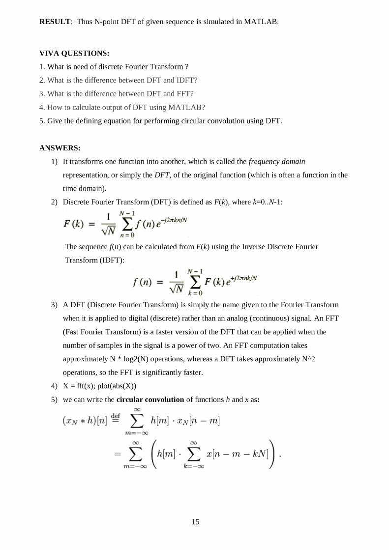
RESULT: Thus N-point DFT of given sequence is simulated in MATLAB.

VIVA QUESTIONS:

1. What is need of discrete Fourier Transform ?

2. What is the difference between DFT and IDFT?

3. What is the difference between DFT and FFT?

4. How to calculate output of DFT using MATLAB?

5. Give the defining equation for performing circular convolution using DFT.

ANSWERS:

1) It transforms one function into another, which is called the frequency domain

representation, or simply the DFT, of the original function (which is often a function in the

time domain).

2) Discrete Fourier Transform (DFT) is defined as F(k), where k=0..N-1:

The sequence f(n) can be calculated from F(k) using the Inverse Discrete Fourier

Transform (IDFT):

3) A DFT (Discrete Fourier Transform) is simply the name given to the Fourier Transform

when it is applied to digital (discrete) rather than an analog (continuous) signal. An FFT

(Fast Fourier Transform) is a faster version of the DFT that can be applied when the

number of samples in the signal is a power of two. An FFT computation takes

approximately N * log2(N) operations, whereas a DFT takes approximately N^2

operations, so the FFT is significantly faster.

4) X = fft(x); plot(abs(X))

5) we can write the circular convolution of functions h and x as:

16

PROGRAM-5 IIR FILTER DESIGN

AIM: To design Chebyshev type-1 IIR filters

(a) Low pass filter.

(b) High pass filter.

(c) Band pass filter.

(d) Band stop filter.


PROGRAM:

%PROGRAM for the design of Chebyshev type-1 low pass digital filter

clc ;

close all ;

clear all ;

format long

rp=input('enter the passband ripple........') ;

rs=input('enter the stopband ripple........') ;

wp=input('enter the passband frequency........') ;

ws=input('enter the stopband frequency........') ;

fs=input('enter the sampling frequency........') ;

w1=2*wp/fs ;

w2=2*ws/fs ;

[n,wn]=cheb1ord(w1,w2,rp,rs) ;

[b,a]=cheby1(n,rp,wn) ;

w=0:0.01:pi ;

[h,om]=freqz(b,a,w) ;

m=20*log10(abs(h));

an=angle(h) ;

subplot(2,1,1) ;

plot(om/pi,m) ;

ylabel('gain in dB -------->') ;

xlabel('(a) normalized frequency--------->') ;

subplot(2,1,2) ;

plot(om/pi,an) ;

xlabel('(b) normalized frequency ---------->') ;

ylabel('phase in radians ------------->') ;

%PROGRAM for the design of Chebyshev type-1high pass filter

clc ;

close all ;

clear all ;

format long





an=angle(h) ;


w1=2*wp/fs ;

w2=2*ws/fs ;

[n,wn]=cheb1ord(w1,w2,rp,rs) ;

[b,a]=cheby1(n,rp,wn,'high') ;

w=0:0.01/pi:pi ;


m=20*log10(abs(h));

subplot(2,1,2) ;

17

subplot(2,1,1) ;

plot(om/pi,m) ;


xlabel('(a) normalized frequency --------->') ;

plot(om/pi,an) ;



%PROGRAM for the design of Chebyshev type-1band pass digital filter

clc ;

close all ;

clear all ;

format long






w1=2*wp/fs ;

w2=2*ws/fs ;

[n]=cheb1ord(w1,w2,rp,rs) ;

wn=[w1,w2] ;

[b,a]=cheby1(n,rp,wn,'bandpass') ;

w=0:0.01:pi ;


m=20*log10(abs(h));

an=angle(h) ;

subplot(2,1,1) ;

plot(om/pi,m) ;



subplot(2,1,2) ;

plot(om/pi,an) ;



%PROGRAM for the design of Chebyshev type-1band stop digital filter

clc ;

close all ;

clear all ;

format long






w1=2*wp/fs ;

w2=2*ws/fs ;

[n]=cheb1ord(w1,w2,rp,rs) ;

wn=[w1,w2] ;

[b,a]=cheby1(n,rp,wn,'stop') ;

w=0:0.1/pi:pi ;


m=20*log10(abs(h));

an=angle(h) ;

subplot(2,1,1) ;

plot(om/pi,m) ;



subplot(2,1,2) ;

plot(om/pi,an) ;


ylabel('phase in radians ------------->')

MODEL GRAPHS:

18

(a) Low pass filter:

Fig: Chebyshev type-1 low pass filter

Parameters:

Enter the pass band ripple : 0.2

Enter the stop band ripple : 45

Enter the pass band frequency : 1300

Enter the stop band frequency : 1500

Enter the sampling frequency : 10000

(b) High pass filter:

Fig: Chebyshev type-1high pass filter

19

Parameters:






(c) Band pass filter:

Fig: Chebyshev type-1band pass filter

Parameters:






20

(d) Band stop filter:

Fig: Chebyshev type-1band stop filter

Parameters:






RESULT: Thus the Infinite Impulse Response(IIR) of the Chebyshev type-1 low-pass, high-pass,

band pass and band reject filters is simulated in MATLAB.

21

VIVA QUESTIONS:

1. Define IIR filters?

2. What is the transfer function of IIR filters?

3. What are different types of IIR filters?

4. Distinguish between frequency response of Chebyshev and Butterworth filters?

5. How to define the order of the IIR filter?

ANSWERS:

1) The impulse responses of recursive filters are composed of sinusoids that exponentially

decay in amplitude. In principle, this makes their impulse responses infinitely long.

However, the amplitude eventually drops below the round-off noise of the system, and the

remaining samples can be ignored. Because of this characteristic, recursive filters are also

called Infinite Impulse Response or IIR filters. In comparison, filters carried out by

convolution are called Finite Impulse Response or FIR filters.

2) Infinite impulse response (IIR) is a property of signal processing systems. Systems with

this property are known as IIR systems or, when dealing with filter systems, as IIR filters.

IIR systems have an impulse response function that is non-zero over an infinite length of

time. This is in contrast to finite impulse response (FIR) filters, which have fixed-duration

impulse responses.

3) IIR filters may be implemented as either analog or digital filters. In digital IIR filters, the

output feedback is immediately apparent in the equations defining the output.

4) Chebyshev filters are analog or digital filters having a steeper roll-off and more passband

ripple (type I) or stopband ripple (type II) than Butterworth filters. Chebyshev filters have

the property that they minimize the error between the idealized and the actual filter

characteristic over the range of the filter, but with ripples in the passband.

5) The order of a recursive filter is the largest number of previous input or output values

required to compute the current output.

22

PROGRAM-6 FIR FILTER DESIGN

AIM: To design Chebyshev type-1 FIR filters

(a) Low pass filter

(b) High pass filter

(c) Band pass filter

(d) Band stop filter.


PROGRAM :

%PROGRAM for the design of FIR low pass, high pass, band pass and band stop filter using

%Chebyshev window

clc;

close all;

clear all;

rp=input('enter the pass band ripple.......');

rs=input('enter the stop band ripple.......');

fs=input('enter the stop band frequency.......');

fp=input('enter the pass band frequency.......');

f=input('enter the sampling frequency.......');

r=input('enter the ripple value in dB....');

wp=2*fp/f;

ws=2*fs/f;

num=-20*log10(sqrt(rp*rs))-13;

dem=14.6*(fs-fp)/f;

n=ceil(num/dem);

if(rem(n,2)==0)

n=n+1;

end

y=chebwin(n,r);

%low pass filter

b=fir1(n-1,wp,y);

[h,o]=freqz(b,1,256);

m=20*log10(abs(h));

subplot(2,2,1);

plot(o/pi,m);

ylabel('gain in dB------>');

xlabel('(a) normalized frequency---->');

title(‘low pass filter’);

%high pass filter

b=fir1(n-1,wp,'high',y);

[h,o]=freqz(b,1,256);

m=20*log10(abs(h));

subplot(2,2,2);

plot(o/pi,m);


xlabel('(b) normalized frequency---->');

title(‘high pass filter’);

23

%band pass filter

wn=[wp ws];

b=fir1(n-1,wn,y);

[h,o]=freqz(b,1,256);

m=20*log10(abs(h));

subplot(2,2,3);

plot(o/pi,m);


xlabel('(c) normalized frequency---->');

title(‘band pass filter’);

%band stop filter

b=fir1(n-1,wn,'stop',y);

[h,o]=freqz(b,1,256);

m=20*log10(abs(h));

subplot(2,2,4);

plot(o/pi,m);


xlabel('(d) normalized frequency---->');

title(‘stop band filter’);

MODEL GRAPHS:

Fig: gain responses of low pass, high pass, band pass and band stop filters

Run:

Enter the pass band ripple....... : 0.03

Enter the stop band ripple....... : 0.02

Enter the stop band frequency....... : 2400

Enter the pass band frequency....... : 1800

24

Enter the sampling frequency....... : 10000

Enter the ripple value in dB.... : 40

RESULT: Thus the Finite Impulse Response(FIR) of Chebyshev low-pass, high-pass, band pass

and band reject filters is simulated in MATLAB.

VIVA Questions:

1. What is the need for a filter?

2. What is meant by cut off in filters?

3. What is FIR filter?

4. What is the transfer function of FIR filter?

Answers:

1. Digital filters that incorporate digital-signal-processing (DSP) techniques have received

a great deal of attention in technical literature in recent years. Although they rarely serve as

anti-aliasing filters (in fact, they need anti-aliasing filters), digital filters merit discussion

here because digital filters offer features that have no counterparts in other filter

technologies.

2. Typically in electronic systems such as filters and communication channels, cutoff

frequency applies to an edge in a lowpass, highpass, bandpass, or band-stop characteristic –

a frequency characterizing a boundary between a passband and a stopband. It is sometimes

taken to be the point in the filter response where a transition band and passband meet, for

example as defined by a 3 dB corner, a frequency for which the output of the circuit is

−3 dB of the nominal passband value. Alternatively, a stopband corner frequency may be

specified as a point where a transition band and a stopband meet: a frequency for which the

attenuation is larger than the required stopband attenuation, which for example may be

30 dB or 100 dB.

3. A finite impulse response (FIR) filter is a type of a signal processing filter whose impulse

response (or response to any finite length input) is of finite duration, because it settles to

zero in finite time.

4. The transfer function for a linear, time-invariant, digital filter can be expressed as a transfer

function in the Z-domain; if it is causal, then it has the form:

25

PROGRAM-7 ECG SIGNAL GENERATION

AIM: To design ECG Signal using MATLAB


PROGRAM :

%PROGRAM for the generation of ECG signal

clc;

close all;

clear all;

x = 1:0.01:3; default = input('press 1 if u want

default ecg signal else 2: ');

if(default ==1)

li = 60/72;

a_pwav = 0.25; d_pwav = 0.09; t_pwav = 0.25; %P-R segment

a_qwav = 0.1; d_qwav = 0.066; t_qwav = 0.166;

a_qrswav = 1.6; d_qrswav = 0.11;

a_swav = 0.25; d_swav = 0.066; t_swav = 0.09;

a_twav = 0.35; d_twav = 0.142; t_twav = 0.3;

a_uwav = 0.035; d_uwav = 0.0476; t_uwav =0.5;

else rate = input ('\n enter the heart

beat rate:'); li= 60/rate;

%p wave specifications fprintf('\n \n pwave

specifications\n'); d = input('enter 1 for default

specification else press 2: '); if( d == 1 )

a_pwav =0.25; d_pwav =0.09; t_pwav =0.25; else a_pwav = input('enter

amplitude ='); d_pwav = input('enter duration

='); t_pwav = input('enter p-r

interval ='); d=0; end

% q wave specifications fprintf('\n \n q wave


specification else press 2: '); if(d == 1) a_qwav = 0.1; d_qwav =0.066; t_qwav = 0.166; else a_qwav = input('enter

amplitude'); d_qwav = input('enter

duration'); t_qwav = input('enter q t

interval'); d = 0; end

%qrs wave specifications fprintf('\n \n qrs wave


specification else press 2: '); if(d ==1)

a_qrswav = 1.6; d_qrswav = 0.11; else a_qrswav =input('enter

amplitude'); d_qrswav =input('enter

duration'); d =0; end

% s wave specifications

26

fprintf('\n \n s wave


specification else 2: '); if(d ==1) a_swav = 0.25; d_swav = 0.066; t_swav = 0.09; else a_swav = input('enter

amplitude'); d_swav = input('enter

duration'); t_swav = input ('enter

interval'); d =0; end

%t wave specifications fprintf('\n \n t wave


apecification else 2: '); if(d ==1) a_twav = 0.35; d_twav =0.142; t_twav = 0.3; else a_twav = input('enter

amplitude'); d_twav = input('enter

duration'); t_twav = input('enter s-t

interval'); d=0; end

% u wave specifications fprintf(' \n \n u wave


specification else 2: ');

if(d == 1) a_uwav =0.035; d_uwav =0.0476; t_uwav = 0.5; else a_uwav =input('enter

amplitude:'); d_uwav = input('enter

duration:'); t_uwav = input('enter

interval'); d=0; end end % p wave putput pwav =

p_wav(x,a_pwav,d_pwav,t_pwav,li);

% q wave output qwav = q_wav(x-

0.10,a_qwav,d_qwav,t_qwav,li);

% qrs wave output qrswav =

qrs_wav(x,a_qrswav,d_qrswav,li);

% s wave specifications swav =

s_wav(x,a_swav,d_swav,t_swav,li);

% t wave specifications twav =

t_wav(x,a_twav,d_twav,t_twav,li);

% u wave specification uwav

=u_wav(x,a_uwav,d_uwav,t_uwav,li);

%ecg output ecg = pwav

+qwav+qrswav+swav+twav+uwav; figure; plot(x,ecg,'r');comet(x,ecg); title('ECG');grid on;

27

MODEL GRAPHS:

Fig: ECG signal generation

Run:

RESULT: Thus the ECG signal is simulated in MATLAB.

VIVA Questions:

Answers:

28

INTRODUCTION TO VHDL

VHDL is an acronym for VHSIC Hardware Description Language (VHSIC is an acronym

for Very High Speed Integrated Circuit).It is a Hardware Description Language that can be used to

model a digital system at many levels of abstraction ,ranging from algorithmic level to the gate

level. The complexity of the digital system being modeled could vary from that of simple gate to a

complex digital electronic system or anything in between. The digital system can also be described

hierarchically. Timing can also be explicitly modeled in the same description.

The VHDL language can be regarded as an integrated amalgamation of following

languages.

Sequential language +

Concurrent language +

Net-list language +

Timing specifications +

Waveform generation language =>VHDL.

The language not only defines the syntax but also defines very clear simulation semantics

for each language construct. Therefore models written in this language can be verified using a

VHDL simulation.

CAPABILITIES:

The following are the major capabilities that the language provides along with the features

that differentiate it from other hardware description languages.

The language can be used as an exchange medium between chip vendors and CAD tool users.

Different chip vendors can provide VHDL descriptions of their components to system

designers. CAD tool users can use it to capture the behavior of the design at a high level of

abstraction of functional simulation.

The language can also be used as a communication medium between different CAD and CAE

tools. For example, a schematic capture PROGRAM may be used to generate a VHDL

description for the design which can be used as an input to a simulation PROGRAM.

The language supports hierarchy, that is, a digital system can be modeled as a set of

interconnected subcomponents.

The language supports flexible design methodologies: top-down, bottom-up or mixed.

It supports both synchronous and asynchronous timing models.

29

Various digital modeling techniques, such as finite state machine descriptions, algorithmic

descriptions and Boolean equations can be modeled using the language.

The language supports three basic different description styles: structural, dataflow and

behavioral. A design may also be expressed in any combination of these three descriptive

styles.

The language is not technology-specific, but is capable of supporting technology specific

features. It can also support various hardware technologies.

BASIC TERMINOLOGY:

A hardware abstraction of a digital system is called an entity. An entity X when used in

another entity Y becomes a component for the entity Y. therefore the component is also an entity,

depending on the level at which you are trying to model.

To describe an entity, VHDL provides five different types of primary constructs called

design units. They are:

Entity declaration.

Architecture body.

Configuration declaration.

Package declaration.

Package body.

ENTITY DECLARATION:

The entity declaration specifies the name of the entity being modeled and lists the set of

interface ports. Ports are signals through which the entity communicates with the other models in

its external environment.

ARCHITECTURE BODY:

The internal details of an entity are specified by an architecture body using any of the

following modeling styles:

As a set of interconnected components (to represent structure).

As a set of concurrent assignment statements (to represent dataflow).

As a set of sequential assignment statements (to represent behavior).

30

CONFIGURATION DECLARATION:

This is used to select one of the many possibly architecture bodies that an entity may have,

and to bind components , used to represent structure in that architecture body, to entities

represented by an entity-architecture pair or by a configuration which reside in a design library.

PACKAGE DECLARATION:

This is used to store a set of common declarations, such as components, types, procedures

and functions. These declarations can then be imported into other design units using a ‘use’ clause.

PACKAGE BODY:

This is used to store the definitions of functions and procedures that were declared in the

corresponding package declaration, and also complete constant declarations for any deferred

constants that appear in the package in the package declaration.

STRUCTURAL MODELING:

In the structural style of modeling, an entity is described as a set of interconnected

components. Example: Half adder. The entity declaration for half adder specifies the interface

ports for this architecture body. The architecture body is composed of two parts: the declarative

part (before the keyword begin) and the statement part(after the keyword begin). Two component

declarations are present in the declarative part of the architecture body. These declarations specify

the interface of components that are used in the architecture body. The declared components are

instantiated in the statement part of the architecture body using component labels for these

component instantiation statements. The signals in the port map of a component instantiated and

the port signals in the component declaration are associated by position (called positional

association). However the structural representation for the Half adder does not say anything about

its functionality. Separate entity models would be described for the components XOR2 and AND2,

each having its own entity declaration and architecture body.

A component instantiated statement is a concurrent statement. Therefore, the order of these

statements is not important. The structural style of modeling describes only an interconnection of

components, without implying any behavior of the components themselves nor the entity that they

collectively represent.

31

DATAFLOW MODELING:

In this modeling style, the flow of data through the entity is expressed primarily using

concurrent signal assignment statements. The structure entity of the entity is not explicitly

specified in this modeling style, but it can be implicitly deduced. In a signal assignment statement,

the symbol <= implies an assignment of a value to a signal. The value of the expression on the

right-hand-side of the statement is computed and is assigned to the signal on the left-hand-side,

called the target signal. A concurrent signal assignment statement is executed only when any signal

used in the expression on the right-hand-side has an event on it, that is, the value for the signal

changes.

BEHAVIORAL MODELING:

The behavioral modeling specifies the behavior of an entity as a set of statements that are

executed sequentially in the specified order. This set of sequential statements, which are specified

inside a process statement, do not explicitly specify the structure of the entity but merely its

functionality. A process statement is a concurrent statement that can appear within an architecture

body. A process statement also has a declarative part (before the keyword begin) and a statement

part (between the keywords begin and end process). The statements appearing within the

statement part are sequential statements and are executed sequentially. The list of signals specified

within the parenthesis after the keyword process constitutes a sensitivity list, and the process

statement is invoked whenever there is an event on any signal in this list.

A variable is assigned using the assignment operator := compound symbol; contrast this

with a signal that is assigned a value using the assignment operator <= compound symbol. Signal

assignment statements appearing within a process are called sequential signal assignment

statements. Sequential signal statements, including variable assignment statements, are executed

sequentially independent of whether an event occurs on any signals in its right-hand-side

expression; contrast this with the execution of concurrent signal assignment statements in the

dataflow modeling style.

32

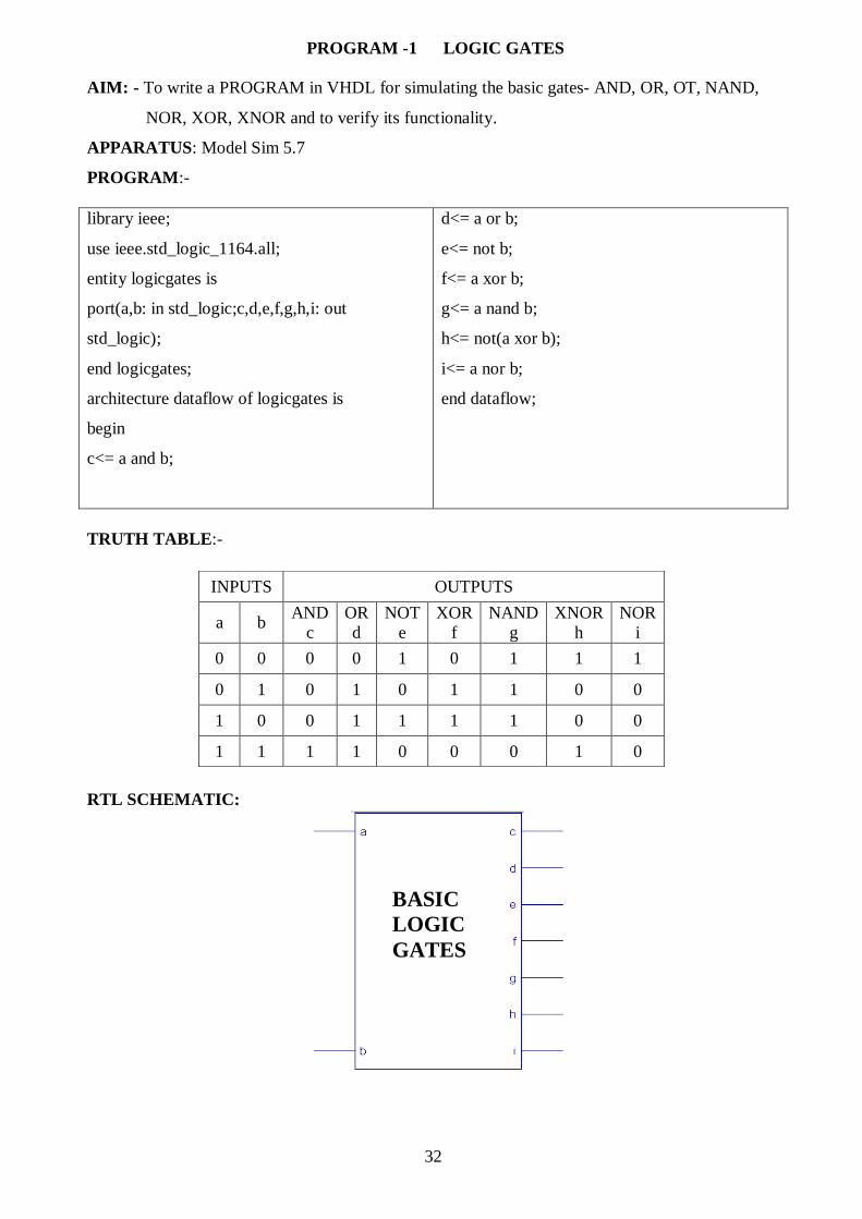
PROGRAM -1 LOGIC GATES

AIM: - To write a PROGRAM in VHDL for simulating the basic gates- AND, OR, OT, NAND,

NOR, XOR, XNOR and to verify its functionality.

APPARATUS: Model Sim 5.7

PROGRAM:-

library ieee;

use ieee.std_logic_1164.all;

entity logicgates is

port(a,b: in std_logic;c,d,e,f,g,h,i: out

std_logic);

end logicgates;

architecture dataflow of logicgates is

begin

c<= a and b;

d<= a or b;

e<= not b;

f<= a xor b;

g<= a nand b;

h<= not(a xor b);

i<= a nor b;

end dataflow;

TRUTH TABLE:-

RTL SCHEMATIC:

INPUTS OUTPUTS

a b AND

c

OR

d

NOT

e

XOR

f

NAND

g

XNOR

h

NOR

i

0 0 0 0 1 0 1 1 1

0 1 0 1 0 1 1 0 0

1 0 0 1 1 1 1 0 0

1 1 1 1 0 0 0 1 0

BASIC

LOGIC

GATES

33

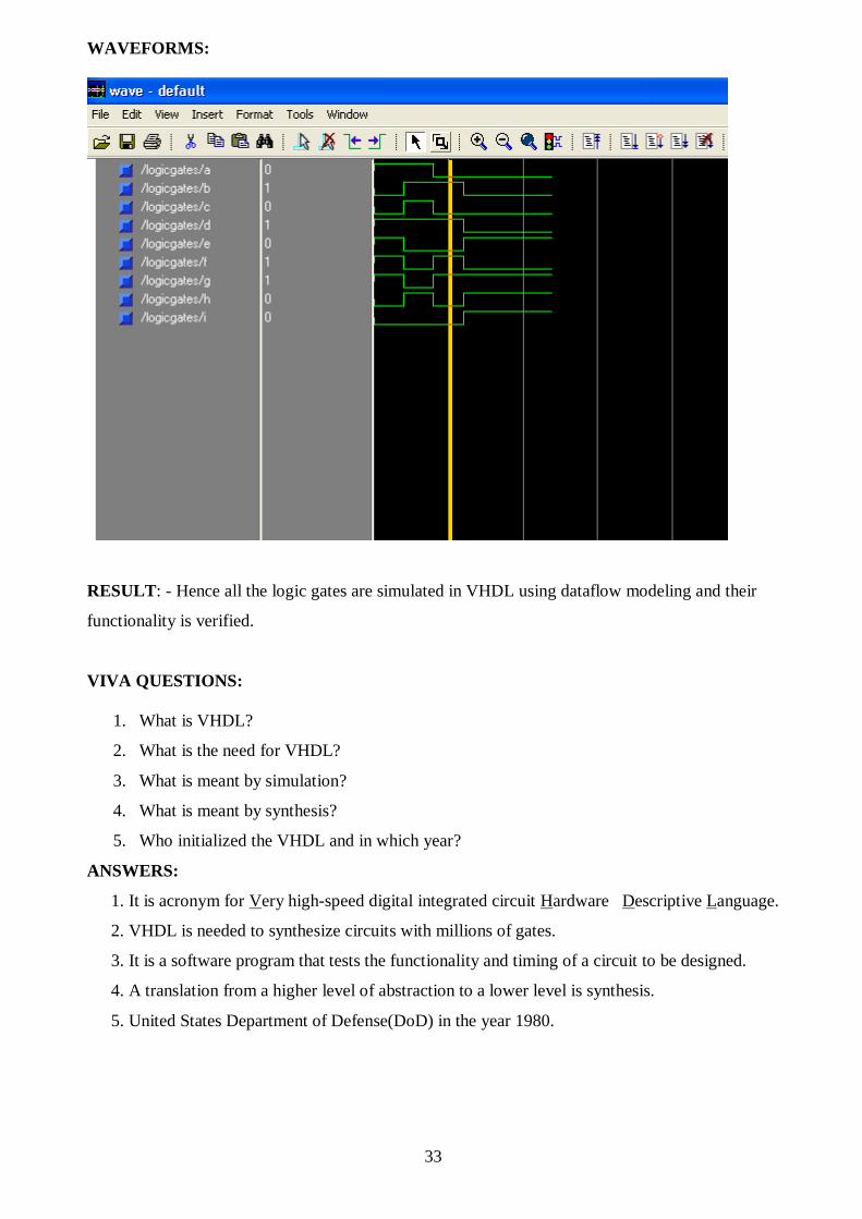
WAVEFORMS:

RESULT: - Hence all the logic gates are simulated in VHDL using dataflow modeling and their

functionality is verified.

VIVA QUESTIONS:

1. What is VHDL?

2. What is the need for VHDL?

3. What is meant by simulation?

4. What is meant by synthesis?

5. Who initialized the VHDL and in which year?

ANSWERS:

1. It is acronym for Very high-speed digital integrated circuit Hardware Descriptive Language.

2. VHDL is needed to synthesize circuits with millions of gates.

3. It is a software program that tests the functionality and timing of a circuit to be designed.

4. A translation from a higher level of abstraction to a lower level is synthesis.

5. United States Department of Defense(DoD) in the year 1980.

34

PROGRAM 2(a) HALFADDER

AIM: - To write a PROGRAM in VHDL for simulating the half adder and to verify its

functionality.


PROGRAM:-

library ieee;


entity halfadder is

port(a,b: in std_logic; s,c: out std_logic);

end halfadder;

architecture dataflow of halfadder is

begin

s<= a xor b;

c<= a and b;

end dataflow;

TRUTH TABLE:-

RTL SCHEMATIC:

INPUTS OUTPUTS

a b Sum

s

Carry

c

0 0 0 0

0 1 1 0

1 0 1 0

1 1 0 1

HALF ADDER

35

WAVEFORMS:

RESULT:- Hence the half adder is simulated in VHDL using data flow modeling and its

functionality is verified .

36

PROGRAM 2(b) FULL ADDER

AIM: - To write a PROGRAM in VHDL for simulating the full adder and to verify

its functionality.


PROGRAM:-

library ieee;


entity fulladder is

port(a,b,c: in std_logic;s,cy: out std_logic);

end fulladder;

architecture dataflow of fulladder is

begin

s<= (a xor b)xor c;

cy<= (a and b) or (b and c) or (c and a);

end dataflow;

TRUTH TABLE:-

INPUTS OUTPUTS

a b c s cy

0 0 0 0 0

0 0 1 1 0

0 1 0 1 0

0 1 1 0 1

1 0 0 1 0

1 0 1 0 1

1 1 0 0 1

1 1 1 1 1

RTL SCHEMATIC:

FULL ADDER

37

WAVEFORMS:

RESULT: - Hence the full adder is simulated in VHDL and its functionality is verified.

VIVA QUESTIONS:

1. What is the assignment operator for i) signal ii) variable ?

2. What is the difference between signal and a variable?

3. Is process used for combinational or sequential logic?

4. What is the difference between function and procedure?

5. Define i) entity ii) architecture.

ANSWERS:

1. ‘<=’ and ‘:=’.

2. Nonstatic values can be passed in VHDL by two ways: signals and variables.

A signal can be declared in package, entity or architecture, while a variable can be declared

within a piece of sequential code. The value of former can be global and the later can be

local.

3. Process can imply combinational or sequential logic, depending upon how it is used.

4. Function can return only one value, whereas procedure can return any no. of values.

5. The entity declaration describes the input and output of the design. It describes the external

interface to the design.

Architecture describes the internal implementation of the design. The architecture body

describes the internal working of the entity and contains any combination of structural,

dataflow, or behavioral descriptions used to describe the internal working of the entity.

38

PROGRAM 3(a) 2x1 Multiplexer

AIM:- To write a code in VHDL for simulating the 2x1 multiplexer and to verify its functionality.


PROGRAM:-

library ieee;


entity mux21 is

port(a,b:in std_logic; s:in std_logic; y:out

std_logic);

end mux21;

architecture beh of mux21 is

begin

process(a,b,s)

begin

case s is

when '0'=>y<=a;

when '1'=>y<=b;

when others=>y<='U';

end case;

end process;

end beh;

TRUTH TABLE:-

SELECT

INPUT OUTPUT

S Y

0 a

1 b

RTL SCHEMATIC:

MUX21

39

WAVEFORMS:

RESULT:- Hence the 2x1 multiplexer is simulated in VHDL and its functionality is verified.

40

PROGRAM 3(b) 4x1 Multiplexer

AIM:- To write a code in VHDL for simulating the 4x1 multiplexer and to observe the waveforms.


PROGRAM:-

library ieee;


entity mux41 is

port(a,b,c,d:in std_logic;s:in std_logic_vector(1

downto 0);y:out std_logic);

end mux41;

architecture beh of mux41 is

begin

process(a,b,c,d,s)

begin

case s is

when "00"=>y<=a;

when "01"=>y<=b;

when "10"=>y<=c;

when "11"=>y<=d;

when others=>y<='U';

end case;

end process;

end beh;

TRUTH TABLE:-

SELECT

DATA

INPUTS

OUTPUTS

S1 S0 Y

0 0 D0

0 1 D1

1 0 D2

1 1 D3

41

RTL SCHEMATIC:

WAVEFORMS:

RESULT:- Hence the 4x1 multiplexer is simulated in VHDL and its functionality is verified.

MUX41

42

PROGRAM 3(c) 8x1 Multiplexer

AIM:- To write a code in VHDL for simulating the 8x1 multiplexer and to verify its functionality.


PROGRAM:-

library ieee;


entity mux81 is

port(x:in std_logic_vector(0 to 7);s:in

std_logic_vector(2 downto 0);y:out std_logic);

end mux81;

architecture structure of mux81 is

component mux41

port(a,b,c,d:in std_logic;s: in std_logic_vector(1

downto 0);y: out std_logic);

end component;

component mux21

port(a,b,s: in std_logic;y: out std_logic);

end component;

signal p1,p2: std_logic;

begin

X1: mux41 port map(x(0),x(1),x(2),x(3),s(1

downto 0),p1);

X2: mux41 port map(x(4),x(5),x(6),x(7),s(1

downto 0),p2);

X3: mux21 port map(p1,p2,s(2),y);

end structure;

43

RTL SCHEMATIC:

MUX41

MUX41

MUX21

44

WAVEFORMS:

RESULT:- Hence the 8x1 multiplexer is simulated in VHDL using structural modeling and its


45

PROGRAM 3(d) 1x8 Demultiplexer

AIM:- To write a code in VHDL for simulating the 8x1 demultiplexer and to verify its

functionality.


PROGRAM:-

Library ieee;


entity dmux81 is

port(a: in std_logic;s: in std_logic_vector(2

downto 0);y: out std_logic_vector(0 to 7));

end dmux81;

architecture dmux of dmux81 is

begin

process(a,s)

begin

y<="00000000";

case s is

when "000"=>y(0)<=a;

when "001"=>y(1)<=a;

when "010"=>y(2)<=a;

when "011"=>y(3)<=a;

when "100"=>y(4)<=a;

when "101"=>y(5)<=a;

when "110"=>y(6)<=a;

when "111"=>y(7)<=a;

when others=>y<="UUUUUUUU";

end case;

end process;

end dmux;

TRUTH TABLE:-

DATA

INPUT

SELECT

INPUTS OUTPUTS

a S2 S1 S0 Y0 Y1 Y2 Y3 Y4 Y5 Y6 Y7

a 0 0 0 a 0 0 0 0 0 0 0

a 0 0 1 0 a 0 0 0 0 0 0

a 0 1 0 0 0 a 0 0 0 0 0

a 0 1 1 0 0 0 a 0 0 0 0

a 1 0 0 0 0 0 0 a 0 0 0

a 1 0 1 0 0 0 0 0 a 0 0

a 1 1 0 0 0 0 0 0 0 a 0

a 1 1 1 0 0 0 0 0 0 0 a

46

RTL SCHEMATIC:

WAVEFORMS:

RESULT:- Hence the 1x8 demultiplexer is simulated in VHDL using behavioral modeling and its


DMUX81

47

VIVA QUESTIONS:

1. What are the basic sections of a VHDL code?

2. Define i) STD_LOGIC_1164 ii) STD_LOGIC_ARITH iii) STD_LOGIC_UNSIGNED

3. What are the rules to be followed while specifying data object names?

4. What are the values the data type STD_LOGIC can assume?

5. How the value of individual SIGNAL and multibit SIGNAL are specified?

ANSWERS:

1. Library, entity and architecture.

2. i) defines the standard for describing the interconnection ii) defines UNSIGNED and

SIGNED types, conversion iii) defines functions to allow the use of

STD_LOGIC_VECTOR types as if they were UNSIGNED types

3. Any alphanumeric character may be used in the name, as well as the ‘_’underscore

character. A name cannot be a VHDL keyword, it must begin with a letter, it cannot end

with an ‘_’ underscore, and it cannot have two successive underscores.

4. ‘U’ --Unintaialized

‘X’ -- Forcing unknown

‘0‘ -- Forcing 0

‘1‘-- Forcing 1

‘Z‘ -- High impedance

‘W‘ -- Weak unknown

‘ L‘ -- Weak 0

‘H‘ --Weak 1

‘- ‘ --Don’t care

5. The value of an individual SIGNAL is specified using apostrophes, as in ‘0’ or ‘1’. The

value of a multibit SIGNAL is given with double quotes.

48

PROGRAM 4(a) SR FLIP FLOP

AIM:- To write a code in VHDL for simulating the SR flip-flop and to verify its functionality.


PROGRAM:-

library ieee;


entity SR is

port(S,R,clk: in std_logic;Q:inout

std_logic:='0';Qb:inout std_logic:='1');

end SR;

architecture ff of SR is

begin

process(S,R,clk)

variable t,tb: std_logic;

begin

t:=Q;

tb:=Qb;

if (clk='0'and clk'event) then

if(S='0'and R='0') then t:=t;tb:=tb;

elsif(S='0'and R='1') then t:='0';tb:='1';

elsif(S='1'and R='0') then t:='1';tb:='0';

elsif(S='1'and R='1') then t:='U';tb:='U';

end if;

Q<=t;

Qb<=tb;

end if;

end process;

end ff;

TRUTH TABLE:-

INPUTS OUTPUTS

S R Q Qb

0 0 Q Qb

0 1 0 1

1 0 1 0

1 1 X X

49

RTL SCHEMATIC:

WAVEFORMS:

RESULT:- Hence the SR flip-flop is simulated in VHDL and its functionality is verified.

SR

FLIPFLOP

S

R

CLK

Q

Qb

50

PROGRAM 4(b) D Flip-Flop

AIM:- To write a code in VHDL for simulating the D flip-flop and to verify its functionality.


PROGRAM:-

library ieee;


entity d_ff is

port(d,clk:in std_logic; Q:inout

std_logic:='0';Qb:inout std_logic:='1’);

end d_ff;

architecture behaviour of d_ff is

begin

process(d,clk)

begin

if (clk='0' and clk'event)then

q<=d;

qb<=not(d);

end if;

end process;

end behaviour;

TRUTH TABLE:-

RTL SCHEMATIC:

INPUTS OUTPUTS

D Q Qb

0 0 1

1 1 0

D_FF

51

WAVEFORMS:

RESULT:- Hence the D flip-flop is simulated in VHDL and its functionality is verified.

VIVA QUESTIONS:

1. What are the various types of operators supported by VHDL?

2. What are the different concurrent assignment statements?

3. What are the different sequential assignment statements?

4. What is the purpose of PROCESS statement?

5. Give the general form of CASE statement.

ANSWERS:

1. Boolean(AND, OR,NAND, NOR,XOR, XNOR), arithmetic(*,/.MOD,REM,-,&), and

relational(=,/<,<=,>,>=)

2. Simple signal assignment, selected signal assignment, conditional signal assignment, and

generate statements.

3. IF statement, CASE statement, and two types of Loop statement(FOR-LOOP and WHILE-

LOOP)

4. To separate the sequential statements from concurrent statements, PROCESS statement is used.

The PROCESS statement appears inside an architecture body, and it encloses other statements

within it. The IF, CASE, and LOOP statements can appear only inside a process.

52

5. CASE expression IS

WHEN constant_value =>

statement;

{statement;}

WHEN constant_value =>

statement;

{statement;}

WHEN OTHERS =>

statement;

{statement;}

END CASE;

53

PROGRAM 5(a) Up-Down Counter

AIM:- To write a code in VHDL for simulating the three bit up/down counter using behavioral

model and to verify its functionality.


PROGRAM:-

library ieee;


use ieee.std_logic_arith.all;

use ieee.std_logic_unsigned.all;

entity bit3_udc is

port(clk,u:in std_logic;a: inout

std_logic_vector(2 downto 0):="000");

end bit3_udc;

architecture beh of bit3_udc is

begin

process(clk,a,u)

begin

if (clk='0' and clk'event) then

if u='1' then a:= a+"001";

elsif u='0' then a:= a+"111";

end if;

end if;

end process;

end beh;

TRUTH TABLE:-

UP/ DOWN q2 q1 q0 Q2 Q1 Q0

0 0 0 0 1 1 1

0 0 0 1 0 0 0

0 0 1 0 0 0 1

0 0 1 1 0 1 0

0 1 0 0 0 1 1

0 1 0 1 1 0 0

0 1 1 0 1 0 1

0 1 1 1 1 1 0

1 0 0 0 0 0 1

1 0 0 1 0 1 0

1 0 1 0 0 1 1

1 0 1 1 1 0 0

1 1 0 0 1 0 1

1 1 0 1 1 1 0

1 1 1 0 1 1 1

1 1 1 1 0 0 0

INPUT PRESENT STATE NEXT STATE

54

RTL SCHEMATIC:

WAVEFORMS:

RESULT:Hence the three bit up/down counter using behavioral model is simulated in VHDL and

its functionality is verified.

UP/DOWN

COUNTER

U

CLK

A(2)

A(1)

A(0)

55

PROGRAM 5(b) SISO & SIPO Shift Register

AIM:- To write a code in VHDL for simulating the Serial In Serial Out(SISO) and Serial In

Parallel Out(SIPO) shift registers using single entity and multiple architectures and to verify its

functionality.


PROGRAM:-

COMPONENT :-

library ieee;


entity D is

port(D,clk: in std_logic;Q:inout std_logic:='0');

end D;

architecture behaviour of D is

begin

process(D,clk)

begin


Q<=D;

end if;

end process;

end behaviour;

SISO 9a:

library ieee;


entity siso_sipo is

port(si,clk: in std_logic;s0,p01,p02,p03:inout

std_logic);

end siso_sipo;

architecture siso_d of siso_sipo is

component D

port(D,clk: in std_logic;Q:inout std_logic:='0');

end component;

begin

D1: D port map(si,clk,p01);

D2: D port map(p01,clk,p02);


D4: D port map(p03,clk,s0);

end siso_d;

SIPO 9b:

architecture sipo_d of siso_sipo is

component D

port(D,clk: in std_logic;Q:inout


end component;

begin

D1: D port map(si,clk,p01);




end sipo_d;

56

RTL SCHEMATIC:

WAVEFORMS:

RESULT:- Hence the Serial In Serial Out and Serial In Parallel Out shift registers using single

entity and multiple architectures is simulated in VHDL and its functionality is verified.

D FF

D FF

D FF

D FF

57

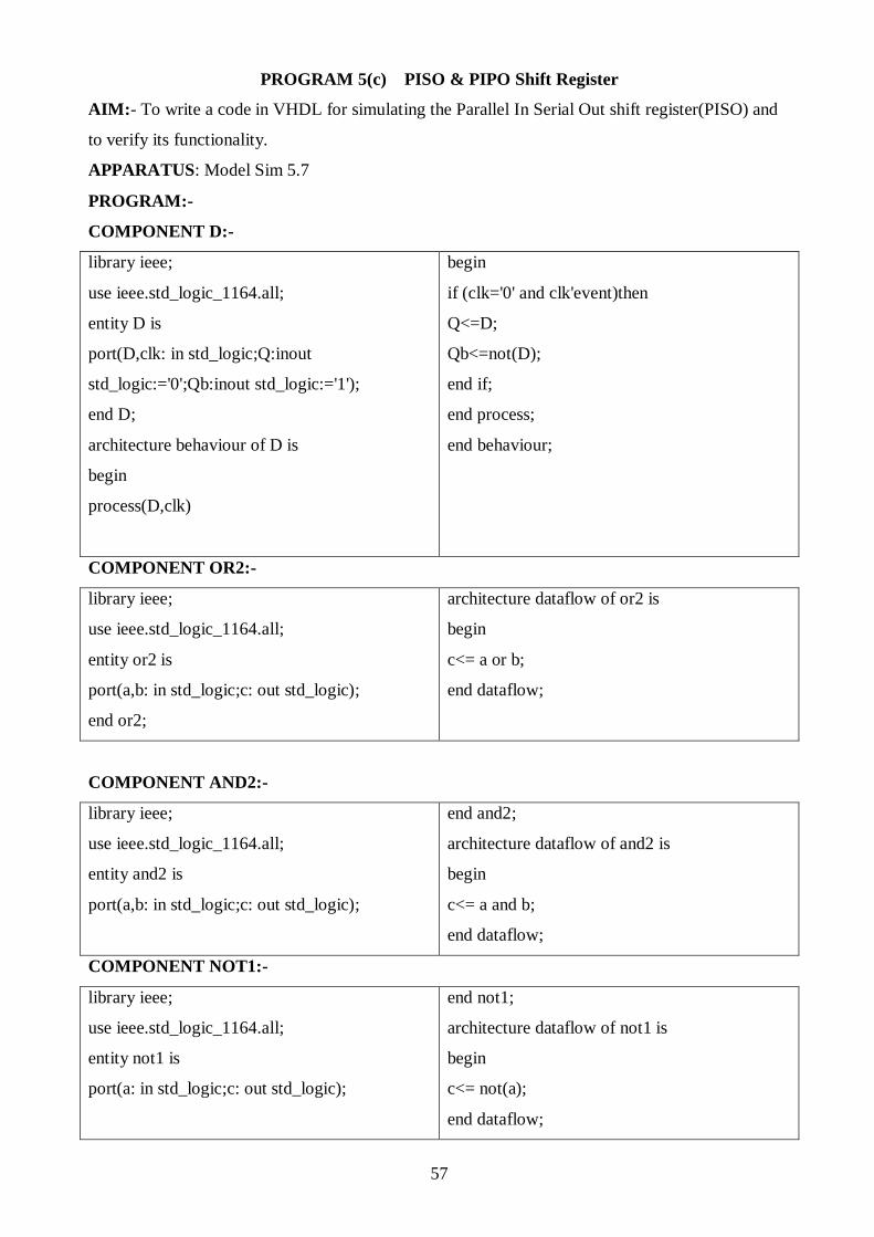
PROGRAM 5(c) PISO & PIPO Shift Register

AIM:- To write a code in VHDL for simulating the Parallel In Serial Out shift register(PISO) and

to verify its functionality.


PROGRAM:-

COMPONENT D:-

library ieee;


entity D is



end D;

architecture behaviour of D is

begin

process(D,clk)

begin


Q<=D;

Qb<=not(D);

end if;

end process;

end behaviour;

COMPONENT OR2:-

library ieee;


entity or2 is

port(a,b: in std_logic;c: out std_logic);

end or2;

architecture dataflow of or2 is

begin

c<= a or b;

end dataflow;

COMPONENT AND2:-

library ieee;


entity and2 is


end and2;

architecture dataflow of and2 is

begin

c<= a and b;

end dataflow;

COMPONENT NOT1:-

library ieee;


entity not1 is

port(a: in std_logic;c: out std_logic);

end not1;

architecture dataflow of not1 is

begin

c<= not(a);

end dataflow;

58

TOP MODULE:-

library ieee;


entity piso is

port(p0,p1,p2,p3,s,clk: in std_logic;Qo: inout

std_logic);

end piso;

architecture piso of piso is

component D



end component;

component and2


end component;

component or2


end component;

component not1

port(a: in std_logic;c: out std_logic);

end component;

signal s1,s2,s3,s4,s5,s6,s7,s8,s9,s10,q1,q2,q3:

std_logic;

begin

n1: not1 port map(s,s1);

D1: D port map(p0,clk,q1,open);

a1: and2 port map(s,q1,s2);

a2: and2 port map(s1,p1,s3);

O1: or2 port map(s2,s3,s4);

D2: D port map(s4,clk,q2,open);




D3: D port map(s7,clk,q3,open);




D4: D port map(s10,clk,Qo,open);

end piso;

59

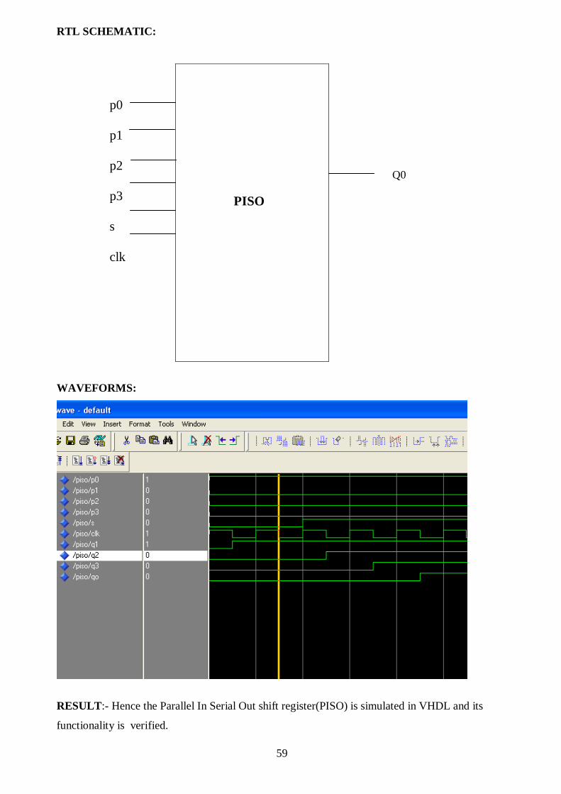
RTL SCHEMATIC:

WAVEFORMS:

RESULT:- Hence the Parallel In Serial Out shift register(PISO) is simulated in VHDL and its


p0

p1

p2

p3

s

clk

Q0

PISO

60

PIPO Shift Register

AIM:- To write a code in VHDL for simulating the Parallel In Parallel Out shift register(PIPO)

and to verify its functionality.


PROGRAM:-

library ieee;


entity pipo is

port(d: in std_logic_vector(3 downto

0);cl,en,clk: in std_logic;q: out

std_logic_vector(3 downto 0));

end pipo;

architecture beh of pipo is

begin

process(cl,clk)

begin

if(cl='1') then

q<="0000" after 5 ns;

elsif(clk'event and clk='1') then

if(en='1') then

q<= d after 5 ns;

end if;

end if;

end process;

end beh;

RTL SCHEMATIC:

PIPO

61

WAVEFORMS:

RESULT:- Hence the Parallel In Parallel Out shift register(PIPO) is simulated in VHDL and its


VIVA QUESTIONS: 1.Give the general form of PROCESS statement.

2. Give the general form of FOR-LOOP statement.

3. Give the general form of WHILE-LOOP statement.

4. What is meant by sensitivity list?

5. How the input and output signals are specified in the ENTITY declaration?

ANSWERS:

1. [process_label:]

PROCESS [(signal name{,signal name})]

[VARIABLE declarations]

BEGIN

[WAIT statement]

[Simple Signal Assignment Statements]

[Variable Assignment Statements]

[IF statements]

[CASE statements]

[LOOP statements]

62

END PROCESS [process_label];

2. [loop_label:]

FOR variable_name IN range LOOP

statement;

{statement;}

END LOOP[loop_label];

3. [loop_label:]

WHILE boolean_expression LOOP

statement;

{statement;}

END LOOP[loop_label];

4. The signals declared inside the parentheses in a PROCESS statement are called

sensitivity list. They indicate which signals the process depends on.

5. Using the keyword PORT.

63

PROGRAM 6

(a) MEALY MACHINE

AIM:- To write a code in VHDL for simulating the Mealy machine(to detect the sequence 10) and



PROGRAM:-

library ieee;


entity mealy is

port(a,clk: in std_logic;z: out std_logic);

end mealy;

architecture beh of mealy is

type state is(s0,s1);

signal p_state,n_state: state;

begin

sm: process(clk)

begin

if rising_edge(clk) then

p_state<=n_state;

end if;

end process sm;

cm: process(p_state,a)

begin

case p_state is

when s0=> if(a='0') then z<='0';

n_state<=p_state;

else z<='0';n_state<=s1;

end if;

when s1=> if(a='1') then z<='0';

n_state<=p_state;

else z<='1';n_state<=s0;

end if;

when others=>z<='0';

n_state<=s0;

end case;

end process cm;end beh;

STATE TABLE:-

PRESENT STATE NEXT STATE OUTPUT(Z)

a=0 a=1 a=0 a=1

S0 S0 S1 0 0

S1 S0 S1 0

64

RTL SCHEMATIC:

WAVEFORMS:

RESULT:- Hence the Mealy machine(to detect the sequence 10) is simulated in VHDL and its


MEALY

65

PROGRAM 6(b) MOORE MACHINE

AIM:- To write a code in VHDL for simulating the Moore machine(to detect the sequence 10) and



PROGRAM:-

library ieee;


entity moore is

port(a,clk: in std_logic;z: out std_logic);

end moore;

architecture beh of moore is

type state is(s0,s1,s2);

signal n_state,p_state: state;

begin

s:process(clk)

begin

if rising_edge(clk) then

p_state<=n_state;

end if;

end process;

d: process(a,p_state)

begin

case p_state is

when s0=>z<='0';

if(a='0') then

n_state<= p_state;

else

n_state<=s1;

end if;

when s1=>z<='0';

if(a='1') then

n_state<=s2;

else

n_state<=p_state;

end if;

when s2=>z<='1';

n_state<=s0;

end case;

end process;

end beh;

STATE TABLE:-

PRESENT STATE NEXT STATE OUTPUT(Z)

a=0 a=1 a=0 a=1

S0 S0 S1 0 0

S1 S2 S1 0 0

S2 S0 S1 1 0

66

RTL SCHEMATIC:

WAVEFORMS:

RESULT:- Hence the Moore machine(to detect the sequence 10) is simulated in VHDL and its


VIVA QUESTIONS:

1. What is meant by component?

2. Give the general form of component instantiation statement.

MOORE

67

3. What is meant by the mode of the PORT?

4. What signal can appear both on the left and right sides of assignment operator?

5. What is the alternative language for digital systems (other than VHDL)?

ANSWERS:

1. A VHDL entity defined in one source code file can be used as a subcircuit in another

source code file. The subcircuit is known as component. A subcircuit must be declared

using a component declaration.

2. Instance_name: component_name PORT MAP (

formal_name = > actual_name {, formal_name => actual_name} );

3. Mode of the PORT specifies whether each port is an input, output, or bidirectional signal.

4. Buffer

5. Verilog

68

7. ADDITIONAL PROGRAM- ARITHMETIC LOGIC UNIT

AIM:- To write a code in VHDL for simulating the Arithmetic Logic Unit(ALU) and to verify its

functionality.


PROGRAM:-

library ieee;


use ieee.std_logic_arith.all;

use ieee.std_logic_unsigned.all;

entity alu is

port(a,b,e: in std_logic;c,d: in integer;s: in

std_logic_vector(2 downto 0);q: out

std_logic;x:out integer);

end alu;

architecture alu1 of alu is

begin

process(e,a,b,c,d,s)

begin

if(e='0')then case s is

when"000"=>q<= a or b;

when"001"=>q<= a and b;

when"010"=>q<= not a;

when"011"=>q<= a xor b;

when"100"=>q<= a nand b;

when"101"=>q<= a nor b;

when"110"=>q<= not(a xor b);

when"111"=>q<= not b;

when others=> null;

end case;

elsif(e='1')then case s is

when"000"=>x<= c+d;

when"001"=>x<= c-d;

when"010"=>x<= c*d;

when"011"=>x<= abs(c);

when"100"=>x<= (c*d)+1;

when"101"=>x<= (c*d)-1;

when"110"=>x<= c+d+1;

when"111"=>x<= c-d-1;

when others=> null;

end case;

end if;

end process;

end alu1;

69

RTL SCHEMATIC:

WAVEFORMS:

RESULT:- Hence the Arithmetic Logic Unit(ALU) is simulated in VHDL and its functionality is

verified.

ALU

department of electronics and communication dsp/vhdl …

Documents