DEPARTMENT OF CHEMISTRY

PHYSICAL CHEMISTRY LABORATORY

CHEMISTRY 444/544LABORATORY MANUAL: WINTER, 2012

1

CONTENTSPage No.

Occupational Health and Safety 3Laboratory Rules and Regulations 4General Fire Orders 6Acknowledgement Form 7Arrangements for Laboratory Sessions 8Reading References 10Plagiarism 12 Laboratory Reports Format 13

Experiments

1 Kinetics of reaction between Fe(III) and SCN by the stopped flow technique 19ˉ

2 Vibrational-Rotational spectra of HCl and DCl 29

3 Thermodynamics of galvanic cells 33

4 Determination of heats of solution from solubility measurements 36

5 The partition coefficient – The equilibrium I- + I2 I3- 38

6 Magnetic susceptibility of solid transition metal compounds 41

7 The dipole moment of chlorobenzene 44

8 Viscosity: Molar mass of a polymer 48

9 Enthalpy of mixing of acetone and water 53

10 Viscosity of gases 57

11 Dissociation constant of CH3COOH from electrical conductivity 61

12 The rate of hydrolysis or inversion of sucrose by polarimetry 66

13 A complex reaction: The bromination of acetone 72

14 Dissociation constant of an indicator by spectrophotometry 77

15 Differential scanning calorimetry 80

2

16 Chemical Oscillations: The Belousov-Zhabotinskii Reaction 87

3

OCCUPATIONAL HEALTH AND SAFETY

YOU are warned that all substances handled and all operations performed in a laboratory

can be hazardous or potentially hazardous. All substances must be handled with care and

disposed of according to laid down procedures. All operations and manipulations must be

carried out in an organised and attentive manner.

In order to assist you in developing good and safe laboratory techniques, a set of Laboratory

Rules and Regulations is attached. You are required to read these and to acknowledge that

you have read and understood them. Additionally, in the laboratory manuals/practical

books and/or pre-practical lectures your attention will be drawn to the correct and safe

handling of specific chemicals/reagents/solvents, and to the correct/safe manner in which

specified laboratory operations must be carried out. These specific instructions and/or

warnings must never be ignored.

4

LABORATORY RULES AND REGULATIONS

1 Students must be present ten minutes before the start of each scheduled laboratory session. Latecomers will be refused entry to the laboratory.

2 No student will be permitted to work in the laboratory outside of laboratory hours except by express permission of the staff member(s) responsible for the session. Never work in a laboratory on your own.

3 Smoking is strictly prohibited in all laboratories and instrument rooms.

4 Do not put anything into your mouth while working in the laboratory. NEVER taste a chemical or solution. Eating is totally PROHIBITED in all laboratories.

5 All students are required to wear a laboratory coat and no student will be permitted to work in the laboratory without one.

6 All students who do not wear conventional spectacles must wear eye protection. Safety glasses must be worn throughout all practical sessions. Students who wear conventional spectacles must have them on at all times when in the laboratory.

7 All students must wear closed shoes in the laboratory, unless permission has been obtained to wear sandals for some medical reason.

8 Apparatus and chemicals are NOT to be removed from the laboratory.

9 Students will find the laboratory bench clean on arrival in the laboratory. The bench at which you work must be left clean when you leave the laboratory at the end of the practical session. Bench tops must be wiped clean. Glassware and other apparatus should be left clean and dry, unless otherwise indicated or instructed.

10 Work areas must at all times be kept clean, and free from chemicals and apparatus which are not required. All glassware and equipment must be returned to its proper place, clean and dry, and in working condition, unless otherwise indicated or instructed.

11 All solids must be discarded into the bins provided in the laboratory. Never throw matches, paper, or any insoluble chemicals into the sinks. Solutions and liquids that are emptied into the sinks must be washed down with water to avoid corrosion of the plumbing. Waste solvents must be placed into the special waste solvent bottles provided.

5

12 Before leaving the laboratory at the end of a practical session make sure that all electrical equipment is switched off, and that all gas and water taps are shut off.

13 Students who break or lose equipment allocated to them will be required to pay for replacements. All breakages or losses must be reported to the teaching assistant in charge.

14 Do NOT heat graduated cylinders or bottles because they will break easily.

15 Any apparatus or glassware which has to be heated must be heated gently at first, increasing the amount of heat gradually thereafter.

16 Balances, spectrophotometers and other expensive equipment must be treated with care and kept clean and tidy at all times.

17 Fumehoods must be used when handling toxic and fuming chemicals. Other operations, such as ignitions, are also carried out in fumehoods. The only parts of the human body which should ever be in a fumehood are the hands - never put your head inside a fumehood.

18 Never leave a laboratory experiment unattended without first consulting the TA in charge.

19 Reagent bottles must be re-stoppered immediately after use. It is absolutely forbidden to introduce anything into reagent bottles, not even droppers. Solutions and reagents taken from bottles must NEVER be returned to the bottles. Do not place the stopper of a reagent bottle onto an unprotected bench top.

20 Laboratory reagents and chemicals must be returned to their correct places immediately after use. Spillage must be cleaned off bottles/containers. Labels must face the front.

21 The use of reagent bottle caps as weighing receptacles is forbidden.

22 Liquids - whether corrosive or not - must be handled with care and spilling on the bench or floor should be avoided. Any spillage must be cleaned up at once - if the liquid is corrosive (acids or bases) call your TA or professor. Never hold a container above eye level when pouring a liquid.

23 When carrying out a reaction or boiling a liquid in a test tube, point the mouth of the test tube away from yourself and others in the laboratory.

6

24 Beware of hot glass and metal. Never handle any item which has been in a flame, a hot oven or a furnace without taking precautions. Use leather/asbestos gloves or tongs, or ask for advice on what to use.

25 Report all accidents, cuts burns, etc., however minor, to your TA or the professor. Eye-wash stations are located in various places in the laboratory. Ensure that you know where the nearest one to your bench is located.

26 A chemical laboratory is not a place for horse-play. Do not attempt any unauthorised experiments. Do not play practical jokes on your classmates. Such things are dangerous and can cause serious injury. Any student found indulging in such activities will be banned from the laboratory, with consequent grade of F for the lab course.

GENERAL FIRE ORDERS

Fire fighting instructions are exhibited in individual laboratories. However, the following orders must always be obeyed.

In the event of a fire

Attack it at once with the appropriate fire fighting equipment and shout for help.

On hearing a fire evacuation alarm

1 Stop normal work immediately.

2 Make safe any apparatus, and material in use, shutting off as necessary any local gas taps/valves, electricity and other potentially dangerous services under your control.

3 Immediately leave the building.

4 Go to the Fire Evacuation Area which for this CHEMISTRY BUILDING is outside to the south west entrance to the building, on the grassed area between the Hall of residence and Science Building 2 (which is the building you are presently).

7

DEPARTMENT OF CHEMISTRY

PORTLAND STATE UNIVERSITY

ACKNOWLEDGEMENT FORM

I, the undersigned (please print full name)

..........................................................................

Student No. ........................................

Identity No. .......................................

do hereby acknowledge having read and understood the documents headed "Occupational Health and Safety" and "Laboratory Rules and Regulations". Furthermore, I accept that contravention(s) of these rules and regulations will lead to my expulsion from the laboratory.

I agree to abide by any additional laboratory regulations or safety rules presented in writing in the practical manuals/books or issued verbally by the INSTRUCTOR-in-charge, or his/her responsible member of staff.

SIGNED ........................................... DATE .......................

8

ARRANGEMENTS FOR LABORATORY SESSIONS

Dates and Times for Practical SessionsPractical sessions will be held only on the specific timetabled day during the winter quarter.

Laboratory sessions will commence promptly. Students are expected to report punctually for each laboratory session. Those arriving late for a practical session may not be admitted to the laboratory. This will result in a mark of zero being recorded for that experiment.

AttendanceA register will be taken each day, and a grade of F may be awarded to students whose attendance records are regarded as unsatisfactory. Each experiment will be marked out of 100; a mark of 0 will be entered in the case of an uncondoned absence. Absences will only be condoned for medical reasons; in such cases a medical certificate must be provided at the next lab session.

DressStudents must wear white laboratory coats and safety glasses at all times while in the laboratory. Open shoes and flip-flops are not considered acceptable dress. The wearing of any headgear in the laboratory is also unacceptable. Sunglasses are not to be worn as a substitute for safety glasses.

AccidentsAny accidents which occur during the laboratory session must be reported immediately to the professor in charge, who is required by law to write an accident report.

BreakagesAny breakages of equipment or glassware must be reported immediately to the TA in charge. The costs of replacement will be debited to the student's fee account.

Waste DisposalCertain experiments generate hazardous waste which must be disposed of according to the instructions provided in the laboratory manual or given by the lecturer in charge.

Laboratory NotebooksStudents are required to have a hardcover notebook in which to write their laboratory reports. Some may prefer to have two lab notebooks so that they can still have one with them after submitting one for grading. These lab notebooks are available in the bookstore. All relevant data, measurements and observations, should be written directly into the lab notebook, and not on some scrap pieces of paper and they transcribed into the lab notebook after the lab session. It is not essential that the lab notebook be clean and neat. Nothing wrong with well-arranged data presentation in a student’s notebook, but this can

8

be more of a product of preparation prior to the session.

Pre-practical Preparation and Report WritingThe key to doing these practicals correctly and expeditiously is your preliminary preparation before coming to the lab session!!

Before coming to the laboratory you should have stated the aim of the experiment you are about to perform that afternoon in your laboratory notebook. In addition, you should have prepared the tables (with the columns appropriately headed) into which you will enter the data you collect during the practical.

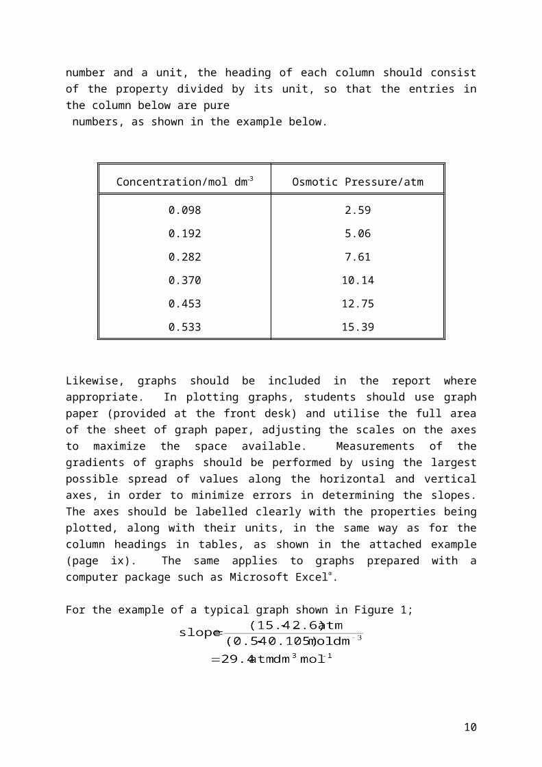
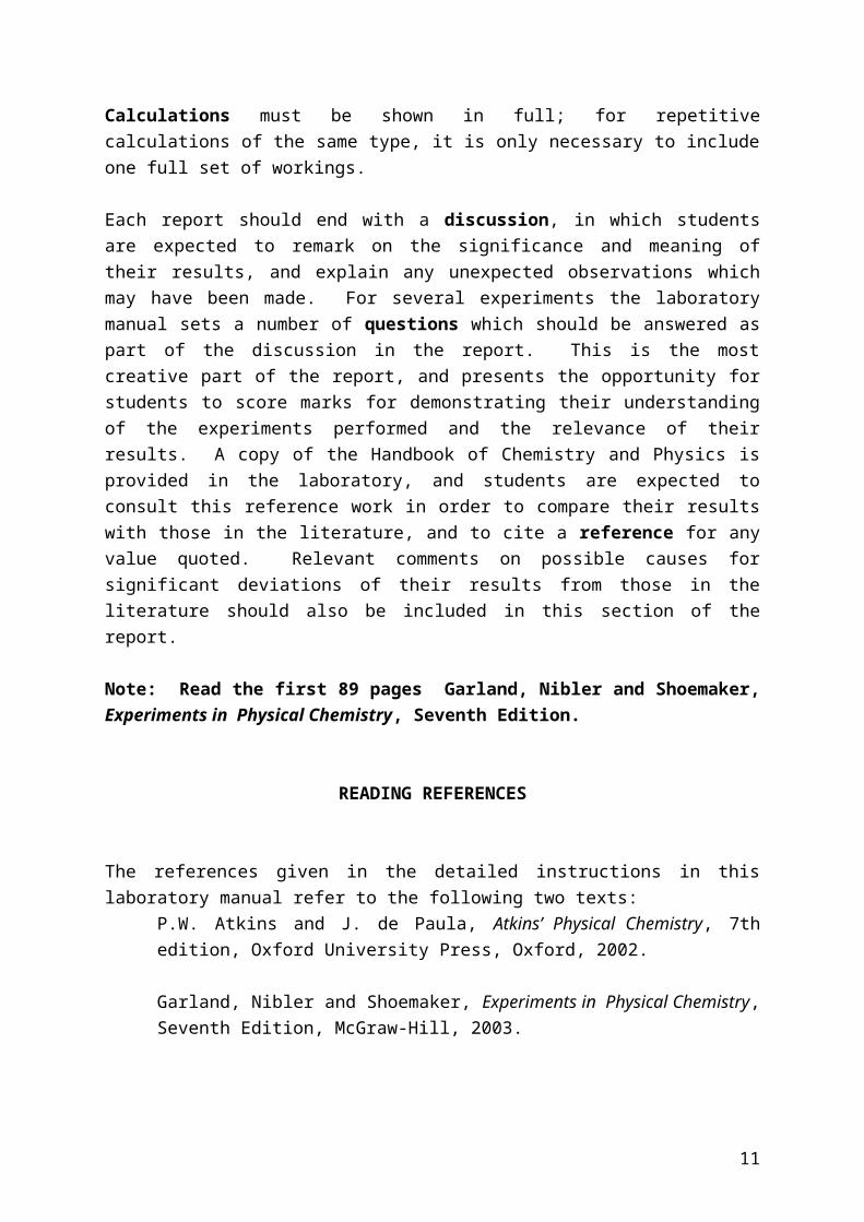
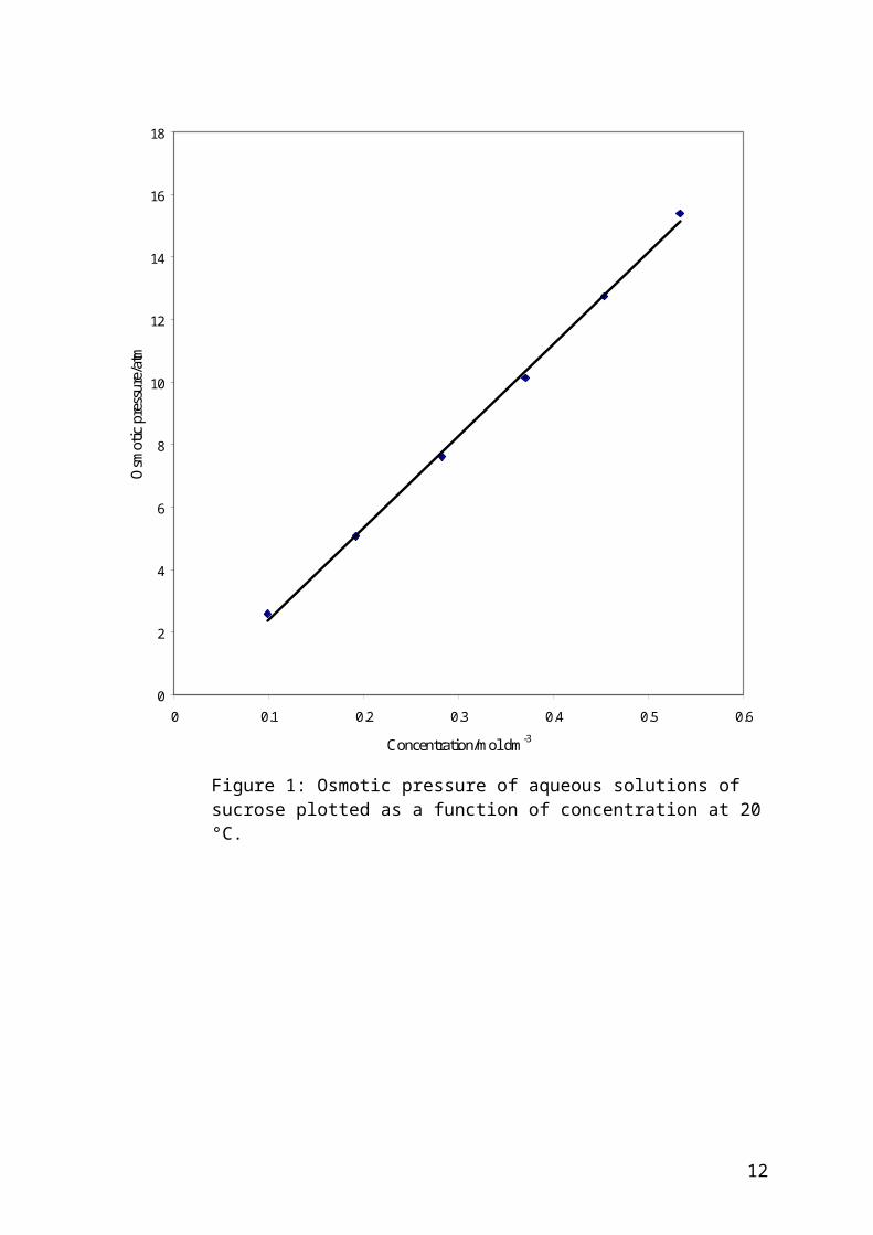
The crude data collected during the laboratory session must be entered directly into the notebook, in ink, in tabular form where appropriate. Each table should contain the appropriate columns of data, each column consisting of a particular physical property. As a physical property is the product of a number and a unit, the heading of each column should consist of the property divided by its unit, so that the entries in the column below are pure numbers, as shown in the example below.

Concentration/mol dm3 Osmotic Pressure/atm

0.098 2.59

0.192 5.06

0.282 7.61

0.370 10.14

0.453 12.75

0.533 15.39

Likewise, graphs should be included in the report where appropriate. In plotting graphs, students should use graph paper (provided at the front desk) and utilise the full area of the sheet of graph paper, adjusting the scales on the axes to maximize the space available. Measurements of the gradients of graphs should be performed by using the largest possible spread of values along the horizontal and vertical axes, in order to minimize errors in determining the slopes. The axes should be labelled clearly with the properties being plotted, along with their units, in the same way as for the column headings in tables, as shown in the attached example (page ix). The same applies to graphs prepared with a computer package such as Microsoft Excel®.

9

For the example of a typical graph shown in Figure 1;

Calculations must be shown in full; for repetitive calculations of the same type, it is only necessary to include one full set of workings.

Each report should end with a discussion, in which students are expected to remark on the significance and meaning of their results, and explain any unexpected observations which may have been made. For several experiments the laboratory manual sets a number of questions which should be answered as part of the discussion in the report. This is the most creative part of the report, and presents the opportunity for students to score marks for demonstrating their understanding of the experiments performed and the relevance of their results. A copy of the Handbook of Chemistry and Physics is provided in the laboratory, and students are expected to consult this reference work in order to compare their results with those in the literature, and to cite a reference for any value quoted. Relevant comments on possible causes for significant deviations of their results from those in the literature should also be included in this section of the report.

Note: Read the first 89 pages Garland, Nibler and Shoemaker, Experiments in Physical Chemistry, Seventh Edition.

READING REFERENCES

The references given in the detailed instructions in this laboratory manual refer to the following two texts:

P.W. Atkins and J. de Paula, Atkins’ Physical Chemistry, 7th edition, Oxford University Press, Oxford, 2002.

Garland, Nibler and Shoemaker, Experiments in Physical Chemistry, Seventh Edition, McGraw-Hill, 2003.

10

0

2

4

6

8

10

12

14

16

18

0 0.1 0.2 0.3 0.4 0.5 0.6

Concentration/mol dm-3

Osm

otic

pre

ssur

e/at

m

Figure 1: Osmotic pressure of aqueous solutions of sucrose plotted as a function of concentration at 20 °C.

11

PLAGIARISM

Plagiarism is defined as the submission or presentation of work, in any form, which is not one’s own without acknowledgement of the source(s). It is an attempt to deceive the reader that the work or ideas presented are your own, whereas, in fact they are the words/ideas of others.

With regard to essays, reports and dissertations, a simple rule should be used when deciding if it is necessary to acknowledge sources. If you obtain information from an outside source, that source must be acknowledged. Another rule to follow is that any direct (verbatim) quotation must be placed in quotation marks and your wording should clearly indicate that the item is not your own work and the source immediately cited. The mere inclusion of the source in a bibliography shall not be considered sufficient acknowledgement.

This applies to all work contributing to assessment, including laboratory reports and projects. All assessed work must be your own individual effort. Copying of laboratory reports, for example, is plagiarism. You may share data, where appropriate, but the calculations, answers to assignment questions and the discussion of results must be your own work.

Work referred to from Internet sources must also be acknowledged as above, with the web address (URL) of the source included and the date it was accessed.

12

Laboratory Reports:

Lab reports must be written INDIVIDUALLY, must be of journal quality, and must follow the JACS format. Online you can also find guidelines on http://www.rose-hulman.edu/~tilstra/ .

Important Dates: To be advised

Before you start an experiment, ask the following questions:1. Do I understand the principle of the experiment?

If not, please go back and read about the experiment. The following resources are available: Experiments in Physical Chemistry by Shoemaker, Garland, Nibler; the web; any physical chem. text.

2. Do I know the experimental setup? If not, go to the lab and find out, ask instructor, web/library search, read the

instrument manual.3. Do I have my lab notebook ready?

The simplest way to keep all the important data is to have a notebook. You are allowed to use the PC’s in the physical chemistry lab to do all the searches and keep good documentation.

Writing all the relevant information about how you are going to do the experiments will help you reduce the time it takes to finish the lab report.

In the Lab: A Checklist Do I have all the equipment necessary to setup the experiment? How do I hook it up and start the experiment? Safety first!!

o Use common sense.o With radiation or high voltage make doubly sure that you are following the

appropriate procedure.o Do not play with open electrical connections or liquid nitrogen.

Prior to collection of datao Check if calibration run needs to be performed.o Check how the data will be saved.o Note the exact instrument model/serial numbers in your notebook.o Take a few minutes to look at the instrumentation manual.o Spend a few minutes to assess sample preparation/purity.o Determine the precision of the instrument.

Data collectiono Decide which variables are fixed and the uncertainties involved in their

measurement.o See how minor perturbations of the experimental conditions affect your data.o Repeat…Repeat…REPEAT…to improve the accuracy/precision of the data.o Record everything in your notebook.

13

After the experimento Shut down the power and clean up the surroundings.o Write down brief notes in the logbook.o Notify instructor if there is any problem.

Analysis of Data Identify the relationship between the independent/dependent variables. Determine both precision/accuracy of measurements Rejection of data: Students test. Fitting the data

o Selection of equation.o Perform linear and/or nonlinear least squares analysis using proper weighting

function. Compare your data to what is expected in the literature. Summarize your conclusions.

Suggest how you might be able to improve the experiment

Laboratory Report Guidelines

Technical reports have several features that are consistent between various fields of study. Below is a list of sections typically found in a technical report. They may exist with slightly different names in different fields. The order in which these are presented may also vary but for the purposes of these guidelines we will use this order, which is the same as the one used in the Journal of the American Chemical Society (JACS).

Abstract

Introduction

Equations

Procedure

Results

Tables

Figures and Plots

Discussion

Conclusion

References

14

The following pages include a more detailed description of each of the sections. Be aware that this is a living document. If some portion of it is inconsistent with your experience, please relay that information.

1.) ABSTRACT

The abstract may be the hardest section of a paper to write. Although it appears at the beginning of an article and is usually the first thing the reader looks at, the abstract should be written last, after the article is complete.

In professional journals, the abstract is often used to identify key features for indexing and so it should contain words that other professionals would use in a literature search. The abstract may appear by itself in a separate publication, and so it must be self-contained. On the other hand, because other professionals read the abstract to get a quick feel if the rest of the article will be of interest to them, it must be concise.

The abstract should contain a brief statement of the problem or purpose of the research. It should indicate the experimental or theoretical plan, summarize the principal findings, and state the major conclusions. It should not add to, evaluate, or comment on conclusions in the text.

The abstract should not cite tables, figures, or sections of the paper. Abbreviations and acronyms should be used sparingly, and should be defined at their first use.

2.) INTRODUCTION

The opening sentence of a paper should state the problem or the purpose of the experiment. Subsequent sentences should provide a concise background and identify the scope and limit of the work.

In professional journals the introduction should also contain the background and/or history of the research project that would be presented. This background should include the citation of pertinent literature, and identify how this work is different or related to the cited literature.

The concepts and their related equations must be developed from an accepted starting point. This means that terms must be defined early in the section, and that the concepts are presented in a logical order such that--when appropriate--they build on each other.

Discussion between equations should connect the equations conceptually. Completeness and clear thought are required in this section. The reader should be convinced that the author(s) know and understand the principles of the experiment.

15

► EQUATIONS

Equations should be offset from the text in some manner, either by indentation or by centering; and numbered. Equations should be numbered sequentially in order of initial appearance; this makes it easy to refer to them at some later point in the text. The terms of equations should be defined the first time those terms appear. It is not necessary to redefine a term every time it appears in an equation. It is not appropriate to use the same notation for different terms in different parts of the text, nor is it correct to use different notation for the same term in different parts of the text.

3.) EXPERIMENTAL PROCEDURE

This section of a report should have sufficient detail about the materials and methods that the audience could repeat the work and obtain comparable results. Identify the materials used, giving information about the purity. Give the chemical names of all compounds and the chemical formulas of compounds that are new or uncommon. Describe your apparatus if it is not standard or commercially available. Describe the procedures you used. Always use third person past tense, e.g. “Acid was added to the solid” and NOT “I added acid to the solid”.

4.) RESULTS

Summarize the data collected. Include only relevant data, but give sufficient detail to justify your conclusions. Use equations, table, and figures for clarity and conciseness. It is often convenient to connect various pieces of information with some discussion. In this case, this section would be called RESULTS AND DISCUSSION

►TABLES

One of the most efficient methods used to communicate technical information is by means of a data table. While you have all seen examples of well-organized, legible data tables, few of you have had a great deal of practice constructing one from scratch. The construction of a good data table requires knowing what the important features are.

I. When to use Tables

Tables are to be used when the data are precise numbers, when there are too many to be presented clearly in the narrative, or when relationships between data can be more clearly conveyed in a table than in the narrative. Tables should supplement, not duplicate, text and figures. If data is not treated theoretically in the report or if the material is not a major topic of discussion, do not present it in tables.

II. How to Construct Tables

A table should consist of at least three columns, and the center and right columns must refer back to the left column. If there are only two columns, the material should be written as narrative. If there are three columns, but they do not relate to each other, perhaps the material is really a list of items and not a table at all.

16

Tables should be simple and concise, but many small tables may be more cumbersome and less informative than one large one. Combining is usually possible when the same column is repeated in separate tables. Use symbols and abbreviations that are consistent among tables and between tables and text.

Numbering Tables: Number tables sequentially with Roman numerals, in order of discussion in the text. Every table must be cited in the text.

Title: Every table must have a brief title that describes its contents. The title should be complete enough to be understood without referring to the text, and it should not contain new information that is not in the text. Put details in footnotes, not in the title.

Column Headings: Every column must have a heading that describes the material below it. Keep headings to two lines, use abbreviations and symbols. Name the parameter being measured and indicate the unit of measure after a comma. A unit of measure is not an acceptable column heading.

Columns. The leftmost column is called the stub column. All other columns refer back to it. Main stub entries may also have subentries that should be indented. Be sure that all columns are really necessary. If there are no data in most of the entries of a column, it probably should be deleted. If the entries are all the same, the column should be replaced with a footnote that says "in all cases, the value was . . . " Do not use ditto marks or the word ditto. Define nonstandard abbreviations in footnotes.

► FIGURES AND PLOTS

Often the most concise and precise way to present data is to plot it. The challenge is knowing what to plot on which axis. An understanding of the theory behind the experiment should provide clues so that the author can determine how to design a plot. Some general rules apply regardless of the content of the report.

The figure, graph or plot should have an appropriate title. Restating the axis labels is NOT an appropriate title.

All axes should be labeled with the parameter being plotted and the units of that parameter. The number of values on the axis and the number of tic marks should be sufficient to make it easy for the reader to identify the x and y values of each data point.

The x-axis is always the independent axis and the y-axis is the dependent axis; that is, the value of the y variable depends on or changes because of a change in the x variable. For example, the concentration of reactants changes because time has passed. It is not true that time has passed because of a change in the concentration of reactants. Consequently, time will be on the x-axis and concentration of reactants will be on the y-axis. By convention, a plot of A versus B means that A is on the y axis and B is on the x-axis.

The plot should not have a legend if there is only one set of data being plotted. Individual data points should be obvious.

17

DO NOT CONNECT THE DOTS!!! It is not appropriate to connect the dots with straight lines (unless it’s a linear regression) because this implies that, between the points for which you took a measurement, the function follows the straight line that you've drawn. This is usually not true. It is appropriate and good to draw a curve on your plot that is the best fit of your data to the functional form that theory predicts. It is appropriate to try to determine the functional form of the data you've presented, however if the theory provides a functional form, use it.

There should be a minimum of emptiness on a plot. If your data covers only a small portion of the plot, expand the axis so that the data fills the plot. There is one exception to this. If part of the purpose of the plot is to identify the value of the y-intercept, the y-intercept should be on the plot.

Plots should be as large as is feasible because if you make a plot too small, all data points will fall on a line. Everything appears linear; even really bad data can be made to look artificially good.

5.) DISCUSSION

After clearly presenting results of your experiments, either as tables or figures, it is necessary to discuss the meaning of those results. The discussion section of a report should be objective. The results of the experiment should be interpreted and (where appropriate) compared with each other. They should be related to the original purpose of the project. In the discussion section, it should be clearly stated whether or not the problem has been resolved. The logical implications of the results should be stated and further study or applications may be suggested. Conclusions should be based on the evidence presented.

6.) CONCLUSION

The conclusion should begin with a restatement of the results. The results should be compared with literature values whenever possible. Any error in the results should be addressed, for example why a plot that--according to theory--should be linear isn't linear. Any possible sources of error should be identified.

7.) REFERENCES

Reference citations come in different styles depending on where the article is being submitted to. For these guidelines we are following the JACS format so familiarize yourself with this and try to use it for your reports. Other formats are also acceptable but it is extremely important that whatever style is used should be used consistently.

18

EXPERIMENT 1

THE KINETICS OF REACTION BETWEEN IRON(III) ANDTHIOCYANATE IONS BY THE STOPPED FLOW TECHNIQUE

Reference: Atkins, Physical Chemistry, 7th Ed., pp. 864-866.

The rates of reaction of metal aquo ions with ligands have been extensively studied. Since these reactions are nearly all fast (complete in <1 second), fast reaction kinetic methods have to be used for measurements. By far the most common of the techniques are stopped flow and temperature jump. In this experiment we use the former method to study the substitution of SCN- into the coordination shell of Fe(III) in water. T-jump, P-jump and flash photolysis may all be used to study this system. The reaction provides a good example since it illustrates many of the factors which have to be taken into account in designing such a kinetic experiment.

Design of the experimentVarious constraints are placed upon the experiment by the chemistry of Fe(III) in water, by the physical chemistry of the solution, and by the experimental method that has been chosen.

Firstly, consider the aqueous solution chemistry of Fe(III) and its reaction with SCN. Fe(III) hydrolyses easily in water, with eventual precipitation of Fe(III) hydroxides. This means that we have to keep the solutions both acidic (pH < 2) and fairly dilute. Since we want to study the substitution into the ion [Fe(H2O)6

3+] by one SCN ion we must not have an excess of the latter ion - to prevent polythiocyanate complexation. Thiocyanate is quite stable in acid solution. Under these conditions the species present in aqueous acid solutions of dilute Fe(III) and SCN can be represented by the equilibria:

k12

[Fe(H2O)63+] + SCN [Fe(H2O)5(SCN)2+] + H2O

k21

KOH Fast KOH Fast equilibrium equilibrium

[H+] [H+] + +

k34[Fe(H2O)5(OH)2+] + SCN [Fe(H2O)4(SCN)(OH)+] + H2O

k43

(KOH = 1.86 x 10-3 M; KOH = 6.5 x 10-5 M; Kc = k12/k21 = 193 M-1 all measured at 25 °C)[Kc = k34/k43]

19

Note that the reaction(s) that we are studying are the forward paths of the equilibria. Note also that there are two substitutions to consider in the mechanism, that is, of the aquo ion and of the monohydroxy aquo ion, and further, that the equilibria are connected by hydrolysis constants. Values for these equilibrium constants can be obtained from the literature.

This leads to the second factor to be considered in the experiment. We need to keep the ionic strength constant (0.5 M here). It is usual to maintain ionic strength with salts such as NaClO4 and LiClO4, and to adjust the acidity with an acid such as HClO4. Obviously the temperature should be constant unless we are measuring activation parameters.

The third constraint arises from the method. Stopped flow is limited in rate to the rate at which we can mix two reagents, and then observe what happens. The shortest dead-times (mixing + viewing time) so far achieved are of the order of several hundred microseconds. In our apparatus we can observe reactions with half lives down to a few milliseconds. It is much easier to study stopped flow kinetics if the reaction profiles (i.e. plots of concentration or absorbance against time) are simple first order (exponential) curves. Thus we usually work under pseudo first order conditions by using a 10-20 fold excess of one reagent. In view of the chemical constraints it is easier here to work with an excess of Fe(III) over SCN . A means of following the course of the reaction is also needed, spectrophotometry is the usual choice where the reagents have characteristic spectra. The red Fe(III) thiocyanate complexes absorb strongly at 460 nm. Another feature of the measurement is that it is possible to measure the optical transmittance of the solution (as a single-beam spectrophotometric measurement), more easily than the absorbance. This is because the latter requires a 100% scale measurement and a log-conversion, remember the Lambert-Beer law. If the changes in transmission are <10% we can assume that the concentration of a reagent is proportional to transmittance. Finally there is the manner in which we record our data. The trace of transmittance against time is displayed on the computer screen and can be printed.

Making up suitable solutionsIn order to help you, stock solutions have been prepared, these are:

A 2.0 x 10-1 M Fe(III) nitrate in 0.1 M HClO4

B 2.0 x 10-2 M NaSCN in 0.2 M NaClO4

C 0.20 M HClO4

D 0.10 M HClO4

E 1.0 M NaClO4

The accurate concentrations of these solutions are given on the reagent bootles.

In the apparatus you will mix a solution of Fe(III) with a solution of SCN. It is suggested that you make up the sodium thiocyanate solution from the following proportions of the stock

20

solutions: 10 cm3 B + 47.80 cm3 E + distilled water to make the volume up to 100 cm3. This gives 2 x 10-3 M NaSCN in a medium of ionic strength 0.5 M.

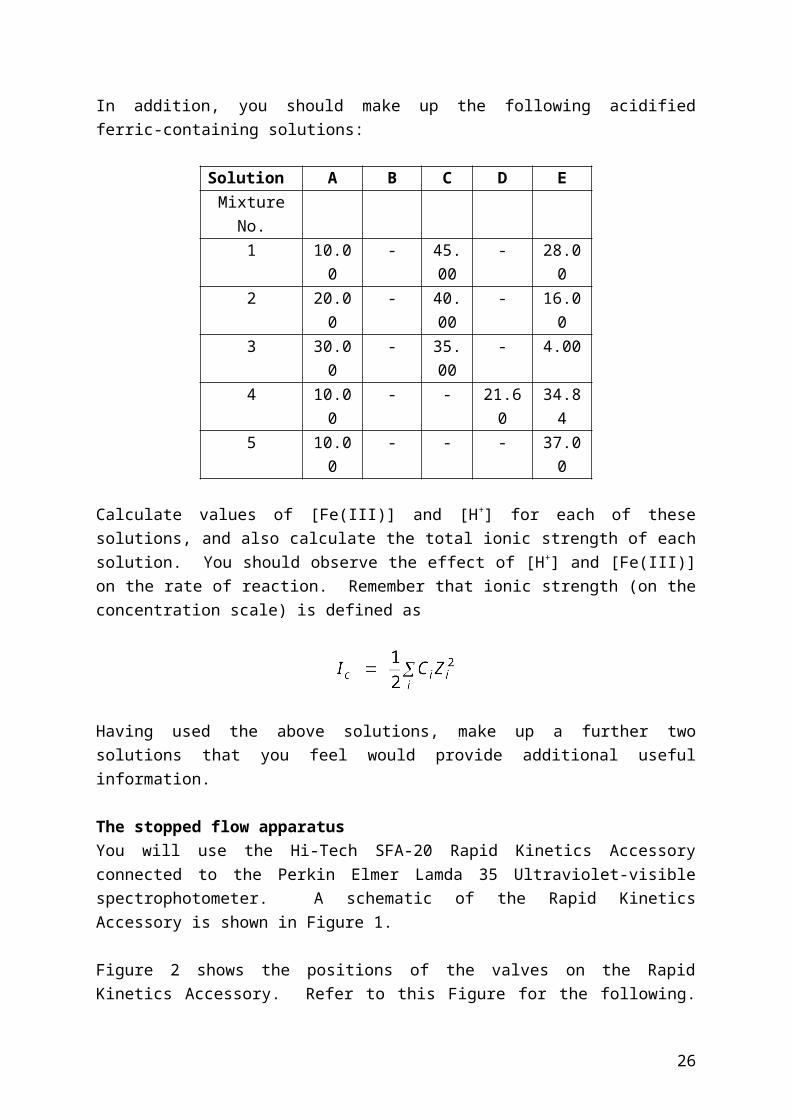
In addition, you should make up the following acidified ferric-containing solutions:

Solution A B C D EMixture No.

1 10.00 - 45.00 - 28.002 20.00 - 40.00 - 16.003 30.00 - 35.00 - 4.004 10.00 - - 21.60 34.845 10.00 - - - 37.00

Calculate values of [Fe(III)] and [H+] for each of these solutions, and also calculate the total ionic strength of each solution. You should observe the effect of [H+] and [Fe(III)] on the rate of reaction. Remember that ionic strength (on the concentration scale) is defined as

Having used the above solutions, make up a further two solutions that you feel would provide additional useful information.

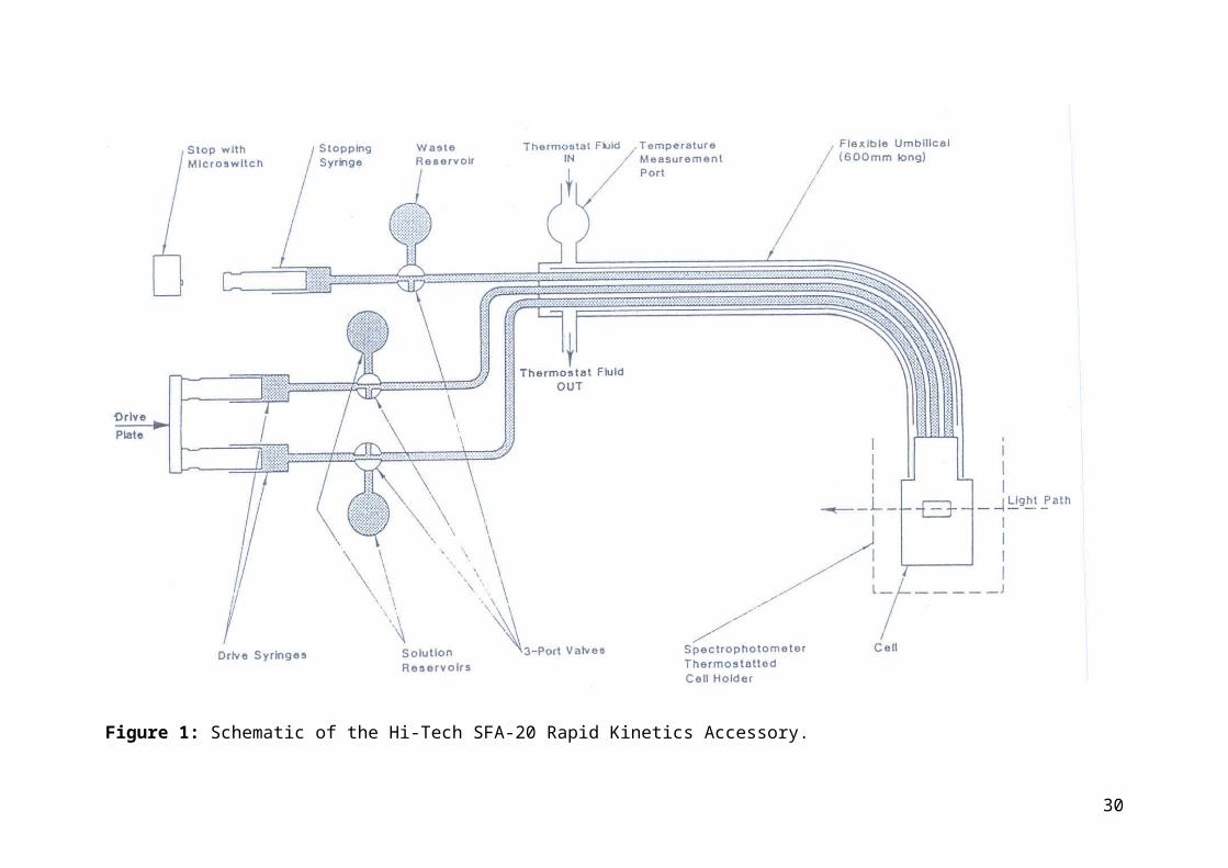
The stopped flow apparatusYou will use the Hi-Tech SFA-20 Rapid Kinetics Accessory connected to the Perkin Elmer Lamda 35 Ultraviolet-visible spectrophotometer. A schematic of the Rapid Kinetics Accessory is shown in Figure 1.

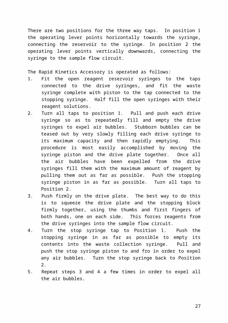
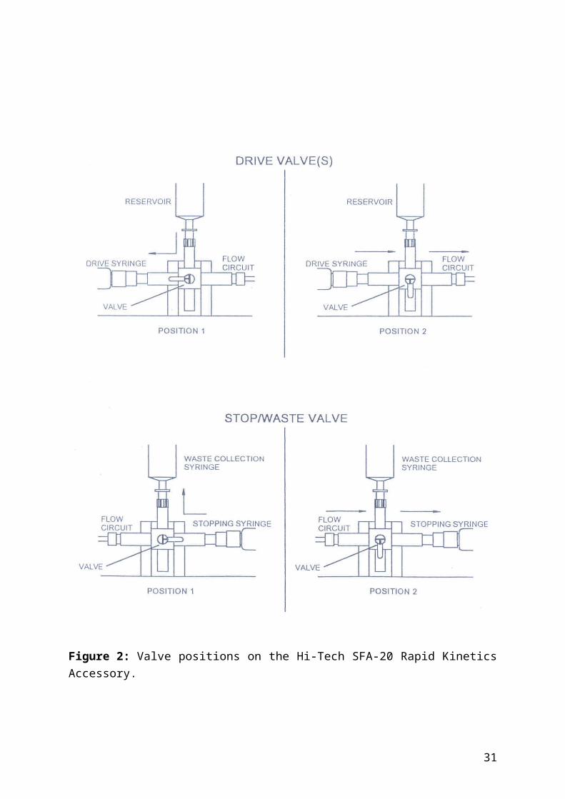
Figure 2 shows the positions of the valves on the Rapid Kinetics Accessory. Refer to this Figure for the following. There are two positions for the three way taps. In position 1 the operating lever points horizontally towards the syringe, connecting the reservoir to the syringe. In position 2 the operating lever points vertically downwards, connecting the syringe to the sample flow circuit.

The Rapid Kinetics Accessory is operated as follows:1. Fit the open reagent reservoir syringes to the taps connected to the drive syringes,

and fit the waste syringe complete with piston to the tap connected to the stopping syringe. Half fill the open syringes with their reagent solutions.

2. Turn all taps to position 1. Pull and push each drive syringe so as to repeatedly fill and empty the drive syringes to expel air bubbles. Stubborn bubbles can be teased out by very slowly filling each drive syringe to its maximum capacity and then rapidly emptying. This procedure is most easily accomplished by moving the syringe piston and the drive plate together. Once all the air bubbles have been expelled from the

21

drive syringes fill them with the maximum amount of reagent by pulling them out as far as possible. Push the stopping syringe piston in as far as possible. Turn all taps to Position 2.

3. Push firmly on the drive plate. The best way to do this is to squeeze the drive plate and the stopping block firmly together, using the thumbs and first fingers of both hands, one on each side. This forces reagents from the drive syringes into the sample flow circuit.

4. Turn the stop syringe tap to Position 1. Push the stopping syringe in as far as possible to empty its contents into the waste collection syringe. Pull and push the stop syringe piston to and fro in order to expel any air bubbles. Turn the stop syringe back to Position 2.

5. Repeat steps 3 and 4 a few times in order to expel all the air bubbles.6. Now that all the air bubbles have been expelled, the unit may be prepared for a run.

Turn all taps to Position 1, fill the drive syringes and empty the stop syringe. Refill the reagent reservoirs as required to prevent further air from being drawn in.

7. To perform a run, turn all the taps to Position 2, start the data capture system, and squeeze the drive plate and stopping block firmly together. The spectrophotometer signal amplitude may vary slightly depending on how hard the drive plate is pushed. For reproducibility adopt the same procedure for each run. If the run is complete in less than a few seconds maintain the pressure until the reaction is complete. If the reaction is slower, release the pressure as soon as the flow stops.

On the SFA-20 Rapid Kinetics Accessory the dead volume between the drive syringes and the observation cell is approximately 1.0 cm3 for both reagents, this amount of reagent will therefore have to be passed through the sample flow circuit before a run can be started. After accounting for the dead volume of the sample flow circuit every subsequent run will only require approximately 200 l of both reagents.

After use the sample flow circuit should be neutralised by washing through with distilled water and ideally being followed by a flush of air, nitrogen or methanol. All the syringe pistons should be pushed right in, or removed if the instrument is not to be used for a long period of time.

ResultsAn exponential curve should be observed because the Fe(III) is in excess and its concentration remains reasonably constant over the course of the reaction (giving a pseudo first order reaction). Plot ln x against t, where x is the distance from the curve to the maximum (levelling off) value at time t. The slope of the line gives the pseudo first order rate constant -kobs.

Determine kobs and t½ for a range of solution concentrations. Firstly work out the observed second order rate constants for each solution. Try plotting these against the reciprocal acid concentration. From this graph you can calculate the rates k12 and k34 in the equilibria

22

depicted at the beginning of the notes. You should also calculate the reverse rate constant k21 from the equilibrium constant Kc quoted. Estimate the accuracy of your data. Calculate Kc (= k34/k43) from Kc, KOH and KOH.

23

Figure 1: Schematic of the Hi-Tech SFA-20 Rapid Kinetics Accessory.

24

Figure 2: Valve positions on the Hi-Tech SFA-20 Rapid Kinetics Accessory.

25

Kinetic analysisSince the position of the equilibrium connecting the FeSCN2+ and Fe(OH)SCN+ species lies far over towards FeSCN2+, there is virtually no accumulation of Fe(OH)SCN+ in the system and the rate of formation of FeSCN2+ = k12[Fe][SCN] + k34[FeOH][SCN].

Since

Rate of formation of

Similarly the rate of destruction of FeSCN2+ is given by

Rate of destruction of FeSCN2+ = k21[FeSCN] + k43[Fe(OH)SCN]

Since [Fe(OH)SCN] =

Rate of destruction of

At equilibrium the rates of formation and destruction of FeSCN2+ must be equal, and

where [Fe]e, [SCN]e and [FeSCN]e represent concentrations of the respective species at equilibrium.

or

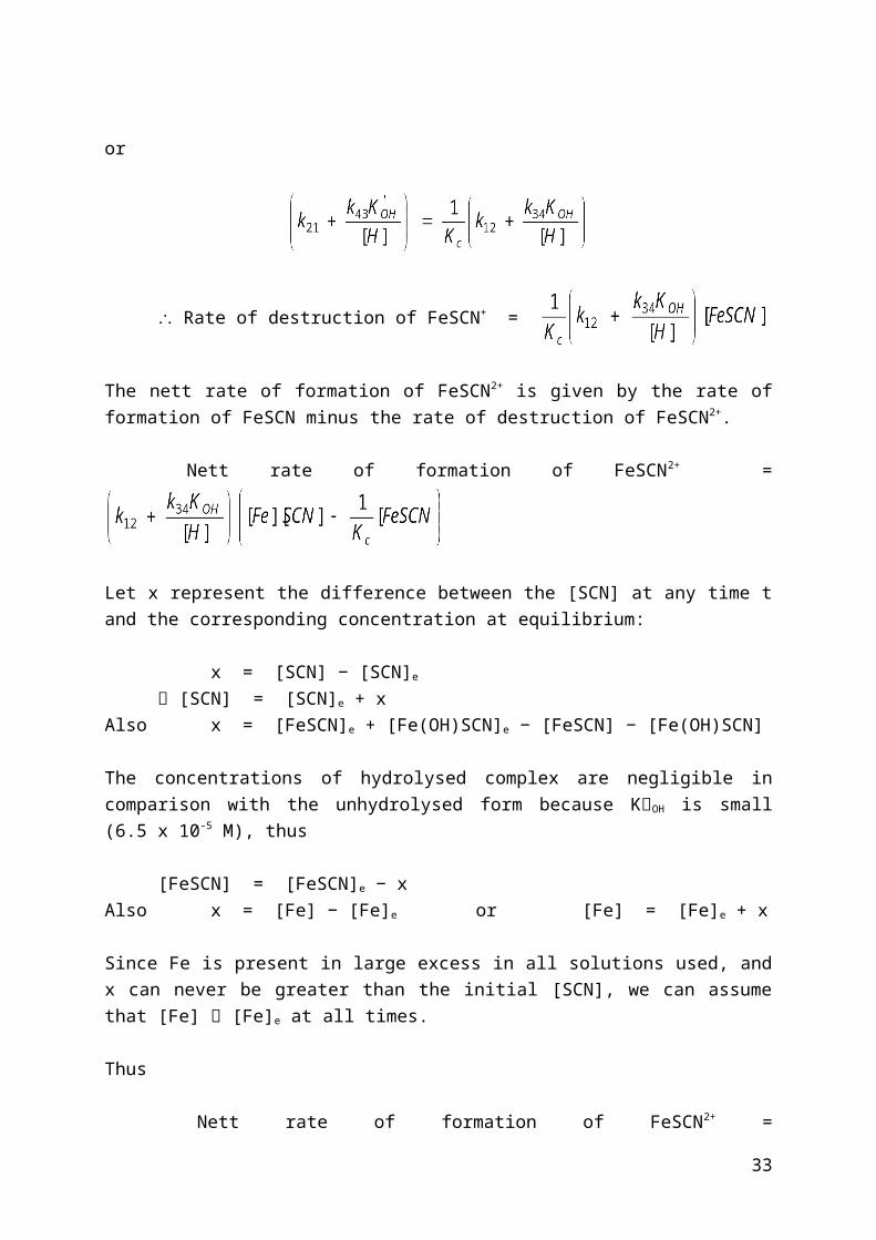
Rate of destruction of FeSCN+ =

26

The nett rate of formation of FeSCN2+ is given by the rate of formation of FeSCN minus the rate of destruction of FeSCN2+.

Nett rate of formation of FeSCN2+ =

Let x represent the difference between the [SCN] at any time t and the corresponding concentration at equilibrium:

x = [SCN] − [SCN]e

[SCN] = [SCN]e + xAlso x = [FeSCN]e + [Fe(OH)SCN]e − [FeSCN] − [Fe(OH)SCN]

The concentrations of hydrolysed complex are negligible in comparison with the unhydrolysed form because KOH is small (6.5 x 10-5 M), thus

[FeSCN] = [FeSCN]e − xAlso x = [Fe] − [Fe]e or [Fe] = [Fe]e + x

Since Fe is present in large excess in all solutions used, and x can never be greater than the initial [SCN], we can assume that [Fe] [Fe]e at all times.

Thus

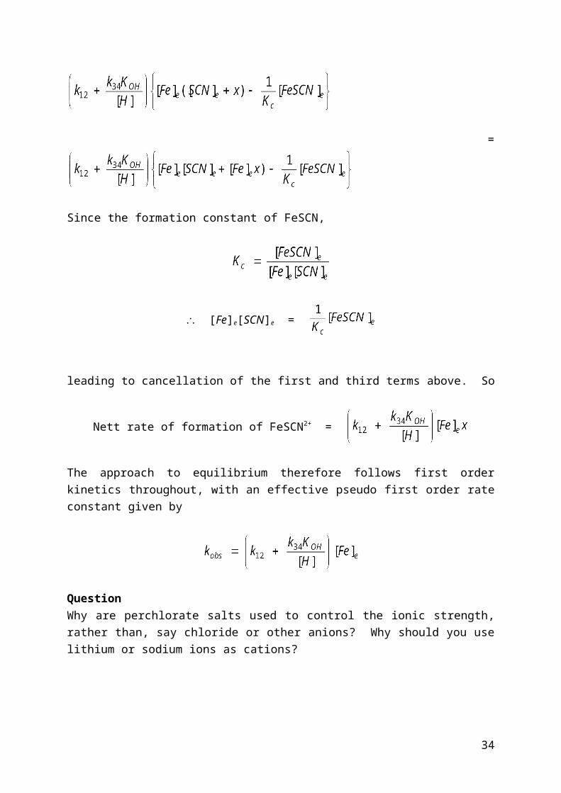
Nett rate of formation of FeSCN2+ =

=

Since the formation constant of FeSCN,

[Fe]e[SCN]e =

leading to cancellation of the first and third terms above. So

27

Nett rate of formation of FeSCN2+ =

The approach to equilibrium therefore follows first order kinetics throughout, with an effective pseudo first order rate constant given by

QuestionWhy are perchlorate salts used to control the ionic strength, rather than, say chloride or other anions? Why should you use lithium or sodium ions as cations?

28

Experiment 2.

VIBRATIONAL-ROTATIONAL SPECTRA OF HCl and DCl

Experiment 37 (page 416) in Shoemaker, et al., 8th edition

Equipment (in 211B):lecture bottles of HCl and DClIR sample cellglass vacuum line with pressure gaugePerkin-Elmer FT-IR w/ data collection PC (in 205)Handouts:Experiment 37 information"Spectrum for Windows" instructions

Introduction:We will determine several spectroscopic and molecular constants of a diatomic molecule, HCl/DCl, from the vibration-rotation spectrum obtained using a Fourier-Transform infrared spectrometer (a Perkin-Elmer model). We are not synthesizing DCl so ignore those sections in Shoemaker et al.

General instructions:The spectra will be recorded with a Perkin-Elmer FTIR located in room 205. Refer to p. 680 in Shoemaker et al. for a brief description of IR spectrometers and, in particular, the discussion regarding Fourier transform instruments.A background scan of the empty cell is first collected. Place the IR cell into the FTIR sample compartment by sliding the end plate of the cell into the mount inside the compartment. Close the sample compartment door. The IR cell is then filled with HCl/DCl using the glass vacuum line located in 211B. Refer to Chapter XIX in Shoemaker, et al. for a discussion of vacuum techniques. Turn all stopcocks slowly and with care. Since over-pressurizing the vacuum line may result in rupture and leakage of the corrosive HCl/DCl gas to the atmosphere, let the TA/instructor actually fill the cell when you are ready. Wear your goggles at all times when in the vicinity of the vacuum line. Record the pressure of the gas sample using the capacitance manometer attached to the vacuum line. A pressure of 150-200 Torr should be sufficient.Make several hard copies of your measured spectrum; one showing all of the absorption lines and a close up of each of the observed branches. A close up showing any splitting in the bands is also useful. It is probably most convenient to use the cursor on the FTIR to ascertain the frequencies of the absorption lines. However, take care to record in your notebook exactly which absorption lines are being measured to avoid confusion later. You can also save your data in ASCII text format (to a diskette or to the CHEM fileserver) so that you can open it in a plotting program, such as KALEIDAGRAPH.

29

Calculations and discussion:Clearly label the R and P branches in the spectra to be included in the final report. Be careful in assigning the branches since your experimental spectrum may be reversed with respect to the example in Shoemaker et al. Assign and label the J" and m values for each absorption line in the spectrum. Some care must be taken in making frequency assignments for peaks that exhibit splitting or asymmetric peaks with shoulders. The spectrometer has sufficient resolution to partially resolve the line splitting due to the presence of 35Cl and 37Cl isotopes. Due to the limited spectral resolution, the expected intensity ratio for the isotopes, 35Cl:37Cl 2:1, is not observed and cannot be used to definitively assign features to either isotope. However, the H37Cl (or D37Cl) lines will be shifted to slightly lower frequencies because the larger reduced mass makes slightly smaller (there is also a smaller effect due to the corresponding decrease in Be). Hence, all of the higher frequency features are due to the 35Cl isotope and the lower frequency features arise from the 37Cl isotope. Indicate how frequency assignments were made for any bands that exhibit splitting and be consistent in which features of split lines are used in subsequent calculations so that only one isotope is used for analysis. Follow the procedure in Shoemaker et al. to make a table of the frequencies and the J" and m assignments. Then make a plot of versus m and use a multiple linear regression to fit the data to equation (10) of Shoemaker et al. (Note this equation includes De, the centrifugal distortion constant. You do not have to perform an F test, as indicated in Shoemaker, but you should comment on the signficance of the De value obtained from your fit.). Show error bars. Be sure to report the correlation coefficient for the least squares fit to the data. To get errors for the fitting parameters using KALEIDAGRAPH, a custom fit must be specified. Select "Curve Fit" "General" "Edit General" and add a "New Fit" to the library. Then you can type in the appropriate curve fit (equation 10) using KALEIDAGRAPH notation (see the "Kaleidagraph Tutorial" handout for some more details about using KALEIDAGRAPH). You must provide initial guesses for all of the fitting parameters. Carry out the calculations described in Shoemaker et al. for your experimental data. When calculating the various molecular constants, be certain that the proper units are being used. Address all of the discussion questions in Shoemaker et al. Be sure to discuss the presence of the Cl isotopes in the experimental spectrum.

Directions for using "Spectrum for Windows" softwareVIBRATIONAL-ROTATIONAL SPECTRA OF HCl Experiment 37 in Shoemaker, et al., 6th edition Instructions:The "Spectrum for Windows" (SFW) software package controls the Perkin-Elmer model 1600 FTIR and is running on a PC connected to the instrument.The data collection computer should be powered on and SFW will start automatically after Windows95 is loaded. Otherwise, SFW can be started by double clicking on the "Spectrum" desktop icon. The user log in dialog box will be displayed. Log in to the program as "144", which can be selected from the list of users in the pull down menu. The password is

30

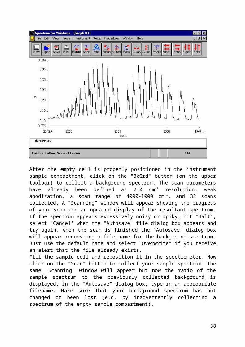
"pchem". If the program is already running, go to the "Setup" menu, select "Change login" and select "144" from the users menu.Place the empty IR cell into the sample compartment by sliding the end plate of the cell into the mount inside the compartment. Close the sample compartment door.The Spectrum main window looks like:

After the empty cell is properly positioned in the instrument sample compartment, click on the "BkGrd" button (on the upper toolbar) to collect a background spectrum. The scan parameters have already been defined as 2.0 cm-1 resolution, weak apodization, a scan range of 4000-1000 cm-1, and 32 scans collected. A "Scanning" window will appear showing the progress of your scan and an updated display of the resultant spectrum. If the spectrum appears excessively noisy or spiky, hit "Halt", select "Cancel" when the "Autosave" file dialog box appears and try again. When the scan is finished the "Autosave" dialog box will appear requesting a file name for the background spectrum. Just use the default name and select "Overwrite" if you receive an alert that the file already exists.Fill the sample cell and reposition it in the spectrometer. Now click on the "Scan" button to collect your sample spectrum. The same "Scanning" window will appear but now the ratio of the sample spectrum to the previously collected background is displayed. In the "Autosave" dialog box, type in an appropriate filename. Make sure that your background spectrum has not changed or been lost (e.g. by inadvertently collecting a spectrum of the empty sample compartment).The sample spectrum will appear in the main graph window. Convert the spectrum to absorbance data by clicking on the "Abs" button in the toolbar. In some cases, multiple spectra may appear in the graph window. Select a specific spectrum by clicking on its file name in the lower left hand corner of the plot. The selected spectrum name will be

31

underlined and in bold. You can then "Close" the selected spectrum from the "File" menu. (Note: if you "halted" a previous spectrum, it may appear in the graph window. Select it and then from the "File" menu select "Close"). A separate step is required to save your data to the C:\144 directory by clicking the "Save" button or selecting the "File" "Save" menu. You can also select "Save As" to save the data as ASCII formatted text, suitable for importing into Kaleidagraph or Excel. Make sure your data is saved so that it may be recalled later for additional analysis.Now manipulate the sample spectrum to expand the region of the spectrum you want to examine. A portion of the spectrum can be selected by holding down the left mouse button and dragging. Then double click in the selected region to zoom in. Alternatively, you can use the "ExpdX/Y" and "PanX/Y" buttons to expand/contract and shift the spectral data. The "Format" button can be used to manually select the range of data you wish to be displayed. The "AutoX" and "AutoY" buttons will autoscale the X- axis (cm-1) and the Y-axis (Absorbance), respectively. The "Back" button returns to the previous scale settings. Make sure that the "View" -> "Overlay/Split Display" -> "Overlay" option is selected or the Y-axis buttons will be grayed out.Use the "VCursr" toolbar button to activate a vertical cursor and read the position, in cm-1, of the observed peaks. Clicking on the button again will remove the cursor. The cursor position can be written on the graph by either double-clicking the left mouse button or selecting the "View" -> "Label Cursor" menu.You can print various views of your spectrum by clicking on the "Print" button. If your spectrum is displayed in color on the screen, it may be printed out as a dash/dotted line. To print the spectrum as a solid line, select "View" -> "Format View", then select "Colors" and select "Spectrum". Now click on the black palette button and then click on the first few spectra (A, B, C, etc.) so that they will be displayed in black. Select "OK" to return to the graph window. You can also select the "Text" button to add a title and other information (e.g. P and R branch labels) to your printout.Make sure you have printed all the views (entire spectrum, single branches, single peaks, etc.) that you will need and have recorded the cm-1 position for all peaks. You can transfer your data to a diskette or to the CHEM network fileserver. Log into CHEM through the "Network Neighborhood" on the desktop or launch the Novell client from the desktop or the "Start" menu.

32

Experiment 3.

Thermodynamics of Galvanic Cells

Introduction

Galvanic cells are electrochemical cells in which an electric current is produced by an electron transfer reaction. The flow of electrons is a result of the electric potential differences that exist between each half reaction. For this experiment the electron transfer reactions were Zn being oxidized to Zn2+ and Fe3+ being reduced Fe2+.

This experiment consisted of two parts. The purpose of the first part was to determine the entropy change (ΔS), the enthalpy of the reaction (ΔH) as a function of temperature and the change in Gibbs energy (ΔG) as a function of temperature. Several fundamental thermodynamic equations were used to derive the working equation for this experiment. These are:

Equation 1: Nernst Equation

Equation 2: dG = -SdT + VdP + idni

Equation 3: ΔG = -nFε

Equation 4: ΔH = ΔG + TΔS

Where n = moles of electrons and F = Faradays constant.

The equation used to determine entropy change in this experiment was

. This equation was derived by substituting equation 3 into equation 2 and

solving for ΔS. Equation 2 simplifies to ΔG= -SΔT under constant pressure and concentration. To calculate ΔS, cell potential should be measured as a function of temperature. Using this

data and the computer program PSIplot 6.0, can be determined graphically by

performing a linear fit to our data. A linear fit can be justified because, according to the Nernst equation, potential should change linearly with respect to temperature if the concentration and pressure are held constant. From this software a linear function and the standard deviation associated with the function can obtained. The experimental value of ΔS is used to plot ΔH and ΔG as a function of temperature.

The purpose of the second part of this experiment is to determine the standard potential (εo) and the activities and activity coefficients versus molarity of the zinc ion. These values can be calculated by collecting data of cell potential as a function of [Zn2+] concentration. The net ionic reaction within our galvanic cell is

33

For this reaction the Nernst equation (equation 1) becomes

If we assume that the activities of the two iron cyanides are similar, the equation can be reduced to

Equation 5:

Knowing that activity is equal to the activity coefficient multiplied by the concentration, this equation can also be written as:

Equation 6:

Where γ = activity coefficient. The above equation, however, has too many unknowns. Therefore, the following equation is used to extrapolate the potential versus concentration data to obtain εo

Equation 7:

This value for along with equation 6 and potential versus concentration data can be used to plot the activity coefficient (γ) as a function of the zinc ion. Equation 5 can be used to plot the activity as a function of the zinc ion.

ExperimentalPart A:

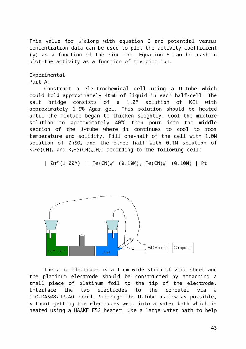
Construct a electrochemical cell using a U-tube which could hold approximately 40mL of liquid in each half-cell. The salt bridge consists of a 1.0M solution of KCl with approximately 1.5% Agar gel. This solution should be heated until the mixture began to thicken slightly. Cool the mixture solution to approximately 40oC then pour into the middle section of the U-tube where it continues to cool to room temperature and solidify. Fill one-half of the cell with 1.0M solution of ZnSO4 and the other half with 0.1M solution of K3Fe(CN)6 and K4Fe(CN)6.H2O according to the following cell:

| Zn2+(1.00M) || Fe(CN)63- (0.10M), Fe(CN)6

4- (0.10M) | Pt

34

The zinc electrode is a 1-cm wide strip of zinc sheet and the platinum electrode should be constructed by attaching a small piece of platinum foil to the tip of the electrode. Interface the two electrodes to the computer via a CIO-DAS08/JR-AO board. Submerge the U-tube as low as possible, without getting the electrodes wet, into a water bath which is heated using a HAAKE E52 heater. Use a large water bath to help minimize room temperature fluctuation. Interface a thermister to the computer via the same CIO-DAS08/JR-AO board and use it to take the voltage and temperature reading at 20 second intervals. Use PSIplot 6.0 software (or any appropriate program) to analyze the potential versus time data.

Part B:Prepare the salt bridge and the ferrocyanide-ferriccynide solutions as in part A. For

this part of experiment, measure the potential as a function of concentration of ZnSO4

solution. Due to limited volume of the cell, try to accomplish the experiment in multiple runs. Approximately 8.0mL (the smallest amount that would still cover the electrodes) of a 0.10M ZnSO4 solution was placed in one half of the cell and diluted with 5.0mL increments of water. After each addition of water, stir the solution and measure the voltage reading. Repeat the procedure 3 more times, each time using a different starting concentration (eg. 1.0M, 0.5M, etc). Measure the voltage from the computer after each dilution. Use PSIplot 6.0 software (or any appropriate program) to analyze the potential versus [Zn2+] data.

Results:Results should include well organized data and plots. Determine ΔS, ΔH and ΔG as a function of temperature. Determine the standard potential (εo) and the activities and activity coefficients versus molarity of the zinc ion.

35

Experiment 4

HEAT OF SOLUTION FROM MEASUREMENTS OF SOLUBILITY

References: Atkins and de Paula, pp. 49-54, 212-214.James and Prichard, pp. 62-64.

Introduction:One of the best known and most useful thermodynamic formulae is the van't Hoff equation, which relates the equilibrium constant of a reaction, K, to the standard enthalpy change of that reaction, ΔHo. It is:

A similar equation can be derived relating the solubility of a solid to its enthalpy of solution:

where S is the solubility in moles per 1000 g of solvent, and ΔHo the standard enthalpy of solution, i.e. the enthalpy change for the solution of benzoic acid in water

C6H5COOH(s) C6H5COOH(aq)

and So = 1 mol kg1. Assuming ΔHo to be constant over the temperature range considered,we get, on integration,

Thus on plotting ln (S/So) against T-1 we should get a straight line of slope ΔHo/R, from which ΔHo can be found.

Experimental Procedure:The thermostat should be set at about 40 °C when you enter the laboratory. A bottle containing a saturated solution of benzoic acid and excess solid benzoic acid will be supplied. Shake the bottle and transfer about 150 cm3 to the conical flask supplied. The solution should contain a few grams of undissolved benzoic acid. Place the flask in a beaker of water

36

which has been heated to about 50 °C and leave it there until it has reached that temperature, keeping the solution well stirred. If the solid disappears more solid benzoic acid should be added. Transfer the flask to the thermostat and again wait until temperature equilibrium has been reached. Stir from time to time.

In the meantime weigh a 100 cm3 conical flask. When the solution is at the correct temperature transfer about 10 cm3 to this flask using the glass wool trap provided. This is to prevent small particles of solid benzoic acid from entering the pipette.

To avoid crystals separating out in the pipette, heat the pipette carefully in a bunsen flame before use. This can be done because the pipette is not being used to deliver a fixed volume.

Weigh the flask plus solution and titrate the benzoic acid against the 0.015 mol dm -3 NaOH supplied, using phenolphthalein as the indicator.

Leave the 200 cm3 flask in the thermostat and drop the temperature to about 35 °C. Repeat the above procedure and do further determinations at 30 °C, 25 °C and 20 °C. Calculate the enthalpy of solution as explained above.

Notes:(i) In this experiment the solution is cooled from a higher temperature because

equilibrium between the solid and the solution is established relatively rapidly in this case. The presence of the solid prevents supersaturation. The establishment of equilibrium when the solid and solution are heated is, however, a very slow process and would take many hours.

(ii) Temperatures should be measured as accurately as possible using the thermometers provided.

Question:Is the sign of ΔHo in accord with Le Chatelier's principle? Discuss.

37

Experiment 5

THE PARTITION COEFFICIENT - THE EQUILIBRIUM I + I2

References: James and Prichard, pp. 227-229.

The Distribution or Partition Law:It was originally supposed that a substance which was soluble in two immiscible liquids would distribute itself in such a way that the ratio of the concentrations in the two layers would be constant at a given temperature. Thus:

This simple law, however, breaks down under certain conditions, namely when A does not exist in the same form in the two liquids. An example is benzoic acid (C6H5COOH) distributed between water and benzene. Benzoic acid exists mainly as a dimer in benzene solution and the partition law found to apply in this case is

Nernst therefore modified the partition law to state that when a solute distributes itself between two immiscible solvents, there exists, for each molecular species, at a given temperature, a constant ratio of partition between the two solvents, and this ratio is independent of any other molecular species which may be present. It can be shown (see any physical chemistry text book) that this statement of the partition law leads to the above equation in the case of the benzoic acid partition.

This experiment involves the partition of iodine between reagent grade hexane and an aqueous solution of potassium iodide. In the hexane layer the iodine exists as I2 molecules, as it does in pure water. In a KI solution, however, the iodine combines with I to form the I3

complex, the following equilibrium being set up,

I2 + I .

The KI and KI3 are insoluble in hexane. The purpose of the experiment is to determine the equilibrium constant of the above reaction. To do this we require the concentration of I 2, I

and in the aqueous layer. The principle of the determination is as follows.

The partition coefficient of I2 between hexane and pure water is obtained. Then iodine is shaken up with hexane and KI solution. The ratio of the concentration of free iodine in the aqueous layer to the concentration of iodine in the hexane layer will be the same as in the case of pure water (by Nernst's partition law above), i.e. it is unaffected by the KI and the fact that some iodine has formed a complex with I. So if we determine the concentration of iodine in the hexane layer by titration we can calculate the concentration of free iodine in the KI solution. A titration of the aqueous layer will yield the total amount of iodine present in this layer, both free and combined in the form of . The concentration of can thus be obtained by difference. If the amount of I originally present in the aqueous layer is known, we can find, again by difference, the amount of I which has not combined to form . Thus we use the fact that the partition law refers to iodine in the same form (i.e. of the same molecular species) in the two layers, and not to the total amount of iodine present. We now have sufficient information to calculate the equilibrium constant.

Experimental Procedure:A saturated solution of iodine in hexane is supplied. Add about 200 cm3 of water to three of the stoppered bottles. Use two burettes to add 25 cm3 of the iodine solution to one bottle; 20 cm3 of solution and 5 cm3 of pure hexane to the second; and 15 cm3 of solution and 10 cm3 of pure hexane to the third. Add about 100 cm3 of the accurately made up 0.12 mol dm-3 KI solution to a further three stoppered bottles and add iodine solution and pure hexane as before.

Shake the bottles well but avoid heating the solutions with your hands. Allow the layers to separate. Titrate the aqueous layer against the sodium thiosulfate solution (0.02 mol dm-

3), by using starch as indicator. The starch indicator solution should only be added towards the end of the titration. Use 50 cm3 of aqueous layer for the first three mixtures and 25 cm3

for the second three. Titrate 5 cm3 of the hexane layer in each case against the sodium thiosulfate solution.

Note:(i) Use the pipette filler provided when pipetting hexane solutions, since hexane vapour

may be harmful.

(ii) The tip of the pipette must pass through the hexane layer to reach the aqueous layer. To prevent the hexane solution from entering the pipette warm the bulb by hand and keep a finger firmly pressed on the back of the pipette.

(iii) It may be necessary to clean the pipette after each filling with hexane solution.

(iv) Make a note of the precise concentrations of the Na2S2O3 and KI solutions provided. This information will be written on the reagent bottles.

Calculate the partition coefficient,

from the data obtained in the absence of I , and find the mean value. Using this value, calculate the equilibrium constant for each of the three determinations involving I in the aqueous phase, and quote a mean value to the appropriate number of significant figures. Note the temperature.

Some assistance with the calculations can be obtained in James and Prichard, p. 228.

EXPERIMENT 6

MAGNETIC SUSCEPTIBILITY OF SOLID TRANSITION METAL COMPOUNDS

References: D. Nicholls, Complexes of the First-Row Transition Elements, pp. 100-111.

D.P. Shoemaker, C.W. Garland, J.W. Nibler, Experiments in Physical Chemistry, 8th Ed., pp. 361 - 370.

If a substance is placed in a magnetic field, the magnetic field strength within the substance will either be greater or smaller than that in the surrounding space. If the intensity is greater, the substance is said to be paramagnetic while if it is smaller the substance is diamagnetic. Diamagnetism is universal in matter while only substances whose molecules or atoms contain unpaired electrons are paramagnetic.

If a substance is placed in a magnetic field of strength, H, (in units of gauss) then the magnetic induction, B, within the substance is given by:

B = H + 4πI (1)

where I is the magnetisation (magnetic moment per unit volume) and is related to the volume magnetic susceptibility, χ, by:

I/H = χ (2)

χ is a dimensionless quantity. The mass magnetic susceptibility, χg, is determined by dividing χ by the density, ρ, of the substance,

χg = χ/ρ (3)

The molar magnetic susceptibility, χm, is obtained by multiplying χg by the molar mass of the substance:

χm = χgM (4)

where M is the molar mass.

χm has units of cm3 mol-1. For paramagnetic substances the molar magnetic susceptibility is of special importance since it is related to the magnetic moment, , of the substance by Langevin'sequation

where N is Avogadro's constant, T the temperature in Kelvin, and k is Boltzmann's constant. Equation (5) may be written as

μ = 2.84(χmT)2 (6)

if μ is expressed in terms of Bohr magnetons, where 1 Bohr magneton = 0.927 x 10 -20 erg gauss-1. (For very accurate work χm must be corrected for small diamagnetic contributions to the susceptibility by the substance.) Quantum mechanically, it can be shown that if it is assumed that only the spins of unpaired electrons contribute to the magnetic moment, μ, (if it is assumed that the orbital moment is small), then μ (in Bohr magnetons) is related to the number of unpaired electrons, n, in the molecules of the substance by the equation:

μ = (7)

Hence, from magnetic susceptibility measurements, n can be estimated.

The Gouy MethodIf a sample is placed so that one end is suspended in a magnetic field and the other end out of the magnetic field, it will experience a force along its length given by:

f = (2)χH2A (8)

where χ is the volume magnetic susceptibility, H the magnetic field strength, and A the cross-sectional area of the sample. If the sample is weighed in this fashion its weight will therefore differ from its weight in the absence of the magnetic field by Δw where:

f = (2)χH2A = gΔw (9)

where g represents the acceleration of gravity and Δw, the difference in mass of the weights used. Hence, χ can be determined from measurement of Δw. In practice, it is convenient to determine the volume magnetic susceptibility of an unknown, χu, by comparing its weight change, Δwu, with that of a substance with known susceptibility, χk, which has a weight change, Δwk, under identical conditions. Then, from equation (9),

also,

(5)

(10)

where wk and wu represent the weights of the known and unknown substances respectively (corrected, of course, for the weight of the tube). ρ represents the effective powder density.

Experimental ProcedureDry the tube and fill it to the mark with the compounds having an unknown magnetic susceptibility. Determine the weight with it suspended between the pole pieces of the magnet and with the magnet removed. Repeat with the standard compound ((NH4)2Fe(SO4)2.6H2O,χg = 32.3 x 10-6 cm3 g-1). Record the room temperature.

Calculate χg, χm, and μ for the standard compound as well as for the unknown compound. Calculate the number of unpaired electrons in your unknown (round off to the nearest whole number). Assuming that electron spin is the only contributor to the magnetic moment, do the values agree with crystal field theory?

Compounds supplied(NH4)2SO4.FeSO4.6H2O, K3Fe(CN)6, Cr2(SO4)3.15H2O, Fe(NO3)3.9H2O, MnSO4.4H2O

Notes1 When filling to the mark, the tube should be tapped repeatedly to ensure that the

solids are packed as tightly as possible in the tube.

2 Care should be taken to ensure that the loaded sample tube hangs freely between the poles of the magnet, and does not touch either pole.

3 If the balance does not swing freely, i.e. if the thread holding the sample tube touches the side of the hole at the base of the balance or the hole through the bench, call the lecturer or demonstrator, who will attend to this.

4 Remove your watch when working near the magnet.

5 Spin-orbit coupling makes a significant contribution to the magnetic moments of the Cr(III) and Fe(II)-containing compounds provided. (See Nicholls.)

(11)

EXPERIMENT 7

THE DIPOLE MOMENT OF CHLOROBENZENE

Reference: Atkins, Physical Chemistry, 7th Ed., pp. 686-696.

A dipole is produced when there is an asymmetric distribution of charge over a molecule. The dipole moment, μ, of a dipole is defined as the charge, q, times the distance, r, by which the charges are separated,

μ = qr (1)

Two types of dipoles are recognised in the molecules of liquids. Some molecules possess permanent dipoles owing to asymmetry of the distribution of electrons and nuclei in the molecule. The other type of dipole is that induced by the presence of an electric field. Molecules are polarizable and the presence of an electric field perturbs the electron distribution in a molecule and produces an induced dipole moment.

When a liquid is placed between the plates of a capacitor, the capacitance is different from that if a vacuum is between the plates, because of the polarizability of the liquid. If Co is the capacitance for a vacuum and C the capacitance for a liquid, then

εr = C/Co (2)

where εr is the relative permittivity or dielectric constant of the liquid. In the presence of an electric field the dipoles of the liquid molecules are partially aligned with the field. If Po is the molar polarizability of the liquid due to permanent dipoles and P I the molar polarizability due to induced dipoles, then the total molar polarizability of the liquid is the sum of the two. For a liquid consisting of non-polar molecules, the induced molar polarizability is related to the molecular polarizability, α, and the dielectric constant by the Clausius-Mossotti equation:

(3)

where M is the molar mass, ρ the density, N Avogadro's constant, and εo is the permittivity of vacuum, i.e. εo = 8.85419 x 10-12 C2 N-1 m-2.

For a liquid consisting of polar molecules, according to Debye, the total molar polarizability, P T, is given by:

(4)

It is therefore apparent that since

(5)then

(6)

If the Boltzmann constant, k, has units of J K-1, μ has units of C m.

It is clear from equation (4) that a plot of PT against T-1 should give a straight line with a slope of Nμ2/9εok from which μ can be determined. An alternate method of determining μ is to measure the polarizability at two widely different frequencies of oscillation of an electric field. One frequency is so low that the molecules have time to retain their orientation with the field and the other so high that no polarization exists. Therefore at the low frequency the molar polarizability is PT while at high frequency the molar polarizability is due only to induced dipoles and is therefore PI. According to Maxwell's theory of light εr = n2 where n is the refractive index and hence the molar refraction Rm of visible light is the same as the induced molar polarizability.

(7)

and therefore the induced molar polarizability can be calculated from measurements of the molar refraction.

The theory of Debye assumes that polar molecules are sufficiently separated so that the interaction among their dipoles is negligible. This condition can only be obtained in the gas phase or in dilute solutions in a non-polar solvent. Consider a polar solute, B, dissolved in a non-polar solvent, A. The polarizability, PAB of the mixture is given by:

(8)

where εr,AB is the dielectric constant of the solution, ρAB the density of the solution, M the molar mass, x the mole fraction, and A and B refer to solvent and solute, respectively. Also,

(9)

where PA and PB are the molar polarizabilities of the pure components. By using equations (8) and (9), PB can be calculated for solutions containing different amounts of B. Then by extrapolation to xB = 0, the molar polarizability (PB)0 at infinite dilution can be obtained.

PI for pure B can be determined from refractive index measurements and hence the orientation molar polarizability, P0, due to the permanent dipoles can be calculated:

(10)

From equation (10) the dipole moment of B can be calculated.

Experimental ProcedurePrepare five solutions of chlorobenzene in cyclohexane with mole fractions of chlorobenzene between 0.05 and 0.3. Prepare the solutions by mass in 50 cm3 volumetric flasks (so that the density of each solution is known). Also fill two 50 cm3 flasks with pure cyclohexane and chlorobenzene, respectively, and weigh. Determine the dielectric constant of each solution and of pure cyclohexane. Note the ambient temperature.

InstrumentationEach student is provided with a dip cell, and should take readings for his own set of solutions.

The leads to the dip cell (i.e. the leads only) should be connected to the LCR bridge. The bridge should be set in C mode (to measure capacitances) and the bridge frequency set at 1 kHz. When the dip cell itself is connected to the instrument via the cell leads, the reading displayed will be the capacitance of the dip cell capacitor with air between the capacitor plates. (A reading of roughly 100 pF will be obtained.) When capacitance readings are taken, care should

be taken to stand well clear of the leads and the cell since the capacitance reading is sensitive to the presence of nearby objects.

It now remains to determine the capacitance of the cell when dipped in the various solutions studied.

CalculationsCalculate PAB (equation (8)) for each solution. Plot PB against xB and by extrapolation to xB = 0, find (PB)0. Calculate PI from values of n and ρ for pure chlorobenzene. Determine the dipole moment of chlorobenzene. Express the answer in Debyes (denoted D). Note that 1 D = 3.336 x 10-30 C m.

NoteCompare the value you obtain for the dipole moment of chlorobenzene with the dipole moment measured in the gas phase. Account for the difference.

EXPERIMENT 8

VISCOSITY: THE MOLAR MASS OF A POLYMER

References: James and Prichard, Practical Physical Chemistry, 3rd Ed., pp. 23-25, pp. 59-60.

Atkins, Physical Chemistry, 7th Ed., pp. 748-750.

If a shearing force is applied to a liquid, the liquid will flow, but at the same time a resistance to this flow will be set up. Consider a liquid flowing along a capillary tube. It has been fairly well established that, if the rate of flow is not too great, the liquid in immediate contact with the wall of the capillary is stationary. The rate of flow increases with the distance from the wall. Let the distance from the wall be z and the velocity of the liquid be u. The frictional force F exerted by a lamina of slower moving fluid on a neighbouring lamina of faster moving fluid is proportional to the area of contact A between the laminae and the velocity gradient du/dz perpendicular to the direction of flow. Thus

where the proportionality constant η is known as the viscosity of the liquid.

NoteThe SI unit of viscosity is kg m-1 s-1. Another commonly used unit is the centipoise (cp). 1 cp = 10-3 kg m-1 s-1.

Measurement of viscosityOne of the most convenient and accurate methods of measuring the viscosity is to measure the rate of flow of a liquid in a capillary tube. It was shown by Poiseuille that the viscosity as defined above is given by

where v is the volume of liquid passing through a narrow tube of length l and radius r in a time t. P is the pressure difference across the two ends of the tube, which causes the flow.

In practice the capillary tube is incorporated in a viscometer; that used in this experiment being the Ubbelohde viscometer. The equation given above shows that if the dimensions of

the capillary are known, the viscosity can be determined. However, it is often difficult to obtain these dimensions to a sufficiently high degree of accuracy and the bore of the capillary tube may not be uniform. A "relative" method is therefore employed in which the time taken for a given volume of the liquid of unknown viscosity to flow through the capillary is compared with the time taken by the same volume of a reference liquid whose viscosity is known.

Molar masses of polymersA sample of polymer will normally not consist of a number of polymer molecules of equal molar mass, such as is the case for a normal substance. Instead the individual polymer molecules will differ in their molar masses and a reasonably continuous range of molar mass is found. The range of molar mass is described by a distribution function P(M), where P(M)dM is proportionalto the number of molecules with molar masses between M and M + dM. In this case

Any molar mass ascribed to a polymer must necessarily, therefore, be an average molar mass. One such average is the "number average molar mass", , where

A second type of molar mass is the "mass average" molar mass.

As the names imply, number average emphasises the number of molecules in a particular molar mass range, while in the mass average the large molecules make a relatively larger contribution. Thus if a polymer solution consisted of a large number of molecules of low molar mass and a few of much higher molar mass, the number average would be low and the mass average much higher. Viscosity determinations do not yield either of the above average molar masses directly but a "viscosity average" molar mass.

which in this case is fairly close to the mass average. "a" is a constant and is discussed below.

Determination of Symbols

η - viscosity of polymer solutionηA - viscosity of pure solvent

ρB is the mass concentration of the polymer, i.e.

expressed in kg m-3. The quantity mB represents the mass of polymer B dissolved in a volume V of the solution.

Investigations into the relationship between the viscosity of polymer solutions and the molar mass of the polymer indicate that

where Κ and a (see above) are constants for the particular polymer/solvent system. For the poly-vinyl alcohol system used in this experiment, Κ = 2.0 x 10 -5 m3 kg-1 and a = 0.76 at T = 25 °C. (M° represents 1 g mol-1.)

The determination of the molar mass of the polymer thus reduces to the determination of the viscosity of the pure solvent and that of the polymer solution at various concentrations.

Experimental ProcedureWash the viscometer well with deionised water. Fill the viscometer with deionised water to the level of the side arm joining the smaller of the lower two bulbs.

NoteAn advantage of this type of viscometer is that it is not necessary to measure out an exact quantity of liquid, in contrast to the Ostwald viscometer (see reference).

Clamp the viscometer vertically in the thermostat. NB: DO NOT CLAMP TOO TIGHTLY. Ensure that the viscometer is immersed up to and including the upper bulb. Leave for at least ten minutes to allow the liquid and viscometer to attain the temperature of the bath. Read the temperature of the bath.

In the meantime pipette 50 cm3 of the stock polymer solution supplied into a 100 cm3

standard flask and make up to the mark with deionised water. Prepare three other progressively more dilute solutions by successive 1:1 dilutions in the same way.

Attach a piece of rubber tubing to the arm of the viscometer containing the capillary tube. Place a finger over the side arm and draw up the liquid into the two bulbs over the capillary tube. Release the liquid and time its passage between the marks above and below the second bulb, using a stopwatch. Repeat the measurement ten times, to allow an estimate of the uncertainty (standard deviation) to be made. Wash the viscometer with deionised water and rinse out a few times with the most dilute solution. Fill with this solution and repeat the measurement obtaining duplicate results only. Repeat for the remaining solutions, once again obtaining duplicate results in each instance.

As can be seen from Poiseuille's equation given on page 10,

since P depends only on the density of the liquid.

In this case the densities can all be taken as that of water and we have

Look up the viscosity of water at 25 °C and find the viscosity of the other solutions.

Plot

as well as

and extrapolate to zero concentration, thus obtaining [η]. Hence, find .

QuestionHow many monomer units are there, on average, in a polymer molecule in the sample studied?

EXPERIMENT 9

ENTHALPY OF MIXING OF ACETONE AND WATER

Reference: Atkins, Physical Chemistry, 7th Ed., pp. 173-174.

The molar enthalpy of mixing, Hmxg/(nA + nB) of two liquids A and B to form a liquid mixture, can be defined as the enthalpy change accompanying the formation of 1 mole of the liquid mixture from the requisite amounts of the two pure liquid components at the same temperature and pressure as the mixture.

In this experiment the molar enthalpies of mixing of various mixtures of acetone and water will be determined.

Experimental ProcedureThe procedure may be divided into two parts:

(a) Determination of the heat of mixing, for each mixture.

(b) Determination of the heat capacity of the calorimeter plus the mixture, for each mixture.

Before proceeding further, ensure that the Beckman thermometer supplied (HANDLE WITH CARE!) is set to read about 2.0 when placed in water at room temperature. If not, readjust (consult demonstrator).

Now support the large boiling tube (the calorimeter vessel) on the magnetic stirrer. Place a magnetic stirrer bar in the tube, add 200.00 cm3 acetone, and then assemble the stopper with the Beckman thermometer and a small test tube passing through the two holes. Ensure that the thermometer bulb is covered by the mixture. Place 4.20 cm3 water in the test tube and ensure that the portion of the test tube containing the water is below the level of the acetone. Switch on the magnetic stirrer, and set the stirring rate to about 300 r.p.m.

(a) Determination of the enthalpy change on mixingRead and record the temperature (the Beckman thermometer can be read to three decimal places) at the end of each minute for 5 minutes. At the end of this period, smash the bottom of the test tube by means of a sharp tap with the iron rod supplied. Ensure that thorough mixing takes place by raising and lowering the broken test tube a few times. The temperature will either rise or fall, depending upon whether the mixing process is exothermic or endothermic, respectively. Continue

reading and recording the temperature at the end of each minute for a further 5 minutes. On graph paper, plot the temperature as ordinate against the time in minutes as abscissa. Join the plotted points. The figure obtained may look more or less as follows - for an exothermic mixing process:

The rise in temperature Tm corresponding to mixture formation may be estimated by extrapolating the lead and trail periods and drawing a vertical line through a point mid-way up. Note that the mixing process takes place relatively rapidly after the test tube is broken.

(b) Determination of the heat capacity of the calorimeter plus the mixtureThis determination is carried out immediately after the measurements described in part (a) are carried out - and makes use of the reaction mixture prepared in part (a). The calorimeter is left as it was at the end of part (a), i.e. the broken test tube and glass fragments, etc., remain as part of the calorimeter.

Read and record the temperature at the end of each minute for 5 minutes. At the end of this period switch on the power to the heating element in the tube, so that a potential difference of exactly 2.50 V and a current of approximately 2 A are applied. Measure the current by means of the digital multimeter provided. Simultaneously, switch on the stop-clock/stopwatch provided. Read and record the potential difference and current on the meters as accurately as possible. Continue reading and recording the temperature of the calorimeter at the end of each minute. When the temperature has risen by approximately 1, switch off the heater, and also the stop-clock/stopwatch. Note the time period over which the heater was activated. Continue reading and recording the temperature as before for a further period of 5 minutes. On graph paper, plot the temperature as ordinate against the time in minutes as abscissa. Join the plotted points. The figure obtained may look more or less as follows:

Note that, in contrast to the situation encountered in the heat of mixing experiment described in part (a), the electrical heating extends over an appreciable time interval. The rise in temperature Th resulting from the electrical heating may be estimated by extrapolation as described in part (a) and shown in the figure above.

More sophisticated and accurate methods exist for correcting calorimetric data for heat exchange with the surroundings. However, the extrapolation method described above is sufficiently accurate for the purposes of this experiment.

Repeat the above procedures for the following mixtures:

(i) Starting with the 200.00 cm3 acetone - 4.20 cm3 water mixture, add successively 7.90 cm3, 7.00 cm3 and 15.80 cm3 of water.

(ii) Starting with 200.00 cm3 water add successively 15.00 cm3 volumes of acetone until a total of 45.00 cm3 is reached.

Note that, particularly after a heat of mixing determination in which the mixture formation is markedly exothermic, it may be necessary to cool the calorimeter vessel before the heat capacity is determined. This may be done by wrapping tissue paper around the vessel and moistening the paper with acetone. Evaporation of the acetone will result in the required cooling effect.

Calculations(a) Calculations of heat capacity

If the potential difference applied to the heater is denoted "V", the current "i", and the time for which the heater was activated is denoted "t", then the heat capacity "Cp" of the calorimeter plus contents is given by

(b) Calculations of enthalpies of mixingThe enthalpy of mixing "Hi" for any particular mixing experiment is given by

(The negative sign is introduced for reasons of sign convention.)

(c) Calculations of molar enthalpies of mixingThe mixtures produced in this experiment are not all produced by mixing the pure components together. Some of the mixtures are prepared by adding more of one of the pure components to an existing mixture from a previous determination. It is therefore necessary to accumulate enthalpies of mixing Hi as calculated in part (b) above in order to calculate the cumulative enthalpy of mixing Hmxg corresponding to formation of any particular mixture from the respective pure components.

Thus,

Hmxg =

If the amounts (mol) of acetone and water in any particular mixture are denoted nac

and respectively, then the molar enthalpy of mixing Hmxg/nTOT is given by

Finally, plot a graph of molar heat of mixing against mole fraction of water. Compare with the figure given in Atkins and comment on the results.

EXPERIMENT 10

VISCOSITY OF GASES

References: D.P. Shoemaker, C.W. Garland, J.I. Steinfeld, J.W. Nibler, Experiments in Physical Chemistry, 8th Ed., pp. 128-135.

Atkins, Physical Chemistry, 7th Ed., pp. 830-832.

In this experiment, the viscosity at room temperature of the following gases: dry air, argon, helium and carbon dioxide, will be determined by measurement of the rate of viscous flow through a cylindrical capillary tube.

Under conditions of laminar flow, the volume rate of flow v (volume per unit time) of a fluid (a gas or a liquid) past a given point in a long cylindrical capillary tube is given by

where r represents the radius of cross-section of the tube, represents the coefficient of viscosity or the "viscosity" of the fluid and dP/dz represents the pressure gradient at any point along the length of the tube. The mean flow velocity v (displacement per unit time) of the fluid at any point along the tube is given by

For a steady flow of a compressible fluid, e.g. a gas, one can show that the molar rate of flow N (moles per unit time) is given by

where P1 and P2 represent the gas pressures at the inlet and outlet of the tube respectively, and L represents the length of the capillary tube. In the derivation of this relationship, ideal gas behaviour is assumed.

In the apparatus used in this experiment the gas contained in a bulb of fixed volume is forced through a capillary tube by mercury flowing into the bulb from an upper reservoir. The time during which the mercury level rises from a lower fiducial mark a to an upper

fiducial mark b is denoted as tab. For any such apparatus of given design and dimensions and containing a constant volume of mercury, the inlet pressure P1 is a definite function of the volume V occupied by the gas in the bulb and tubing leading to the capillary; P2 is a constant (atmospheric pressure). The time required for the mercury meniscus to rise from mark a to mark b is

(1)K

The quantity K depends only on the dimensions L and r of the capillary tube and the geometry of the apparatus used. It can therefore be regarded as an "apparatus constant". While it is possible to determine K from capillary dimensions and measurements of P1 as a function of V, more satisfactory results can be obtained by determining K from the time of flow of a gas of known viscosity.

The above theory is based on the assumption that the flow of gas in the capillary tube is laminar. For fluid flow to be laminar, the flow velocity must be small. An important quantity in hydrodynamics is the so-called Reynolds number R. For flow through a long, round, straight tube

(2)

where represents the density of the fluid. R is a dimensionless quantity. It is found empirically that laminar flow is always obtained in such a tube when the Reynolds number is less than 1 000 regardless of the magnitude of any of the individual variables, r, , and . Laminar flow can be obtained with a Reynolds number as high as 10 000 or even 25 000 if sufficiently careful attention is given to the smoothness of the walls and to the shape of the inlet, but ordinarily turbulent flow is obtained with Reynolds numbers in excess of a few thousand.

The flow velocity profile in the major portion of the capillary tube is of parabolic shape. The gas directly adjacent to the walls of the capillary tube will (ideally) be stationary, while the gas at the centre of the tube will be moving at a velocity vmax = 2 . At the inlet of the tube the velocity profile is uniform. It follows that the gas needs to travel through a certain length of tubing (say L) before the parabolic velocity profile is fully established. Experiments have shown that the length of this transition region is given approximately by the equation

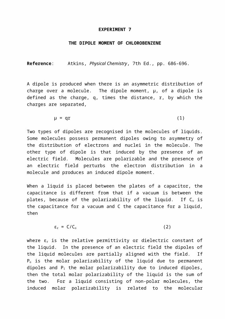
(3)

Since equation (1) does not apply accurately within this transition region, it is necessary that L should be small in comparison with L - for accurate determination of viscosity.

Slip CorrectionThe assumption that fluid in contact with the walls of the capillary is stationary under conditions of laminar flow is well founded for laminar liquid flow. For laminar gas flow the assumption breaks down when the mean free path of the gas molecules l is not negligibly small in comparison with the apparatus dimensions, e.g. the radius r of the capillary tube. This situation can arise when the gas is at very low pressure, or when the gas is at ordinary pressures but the capillary is of very small diameter. In such circumstances, gas viscosities appear to be lower than when measured under ordinary conditions. The gas behaves as though it were "slipping" at the capillary walls, rather than having zero velocity at the walls. If equation (1) yields the "apparent viscosity" app, the true viscosity can be obtained from the equation

(4)

Other corrections for kinetic energy and non-linear effects in rapidly moving fluids are sometimes needed. However, with the present apparatus such effects are very small and can be neglected.

Experimental ProcedureMeasure and record the ambient temperature and barometric pressure. Connect the required sample gas to the open tube on the left-hand side of the apparatus. Open the relevant taps on the apparatus and needle valve on the gas cylinder (if the sample gas is obtained from a gas cylinder), and allow the sample gas to enter the pear shaped bulb, forcing the mercury below the lower fiducial mark. When air is being used, this is pumped into the apparatus by use of the rubber hand pump provided, and the air should be routed through the U-tube containing Mg(ClO4)2 drying agent for removal of water vapour. When gases are admitted to the apparatus from gas cylinders, the valve on the gas cylinder must be opened very carefully to avoid surges of mercury in the apparatus.

When the bulb has been filled with the sample gas and the mercury level is below the lower fiducial mark, then the inlet tap/s must be closed. Examination of the apparatus to determine the nature of the venting tap/s above the pear-shaped bulb is advisable before the flushing or venting procedure is begun. Either two separate taps will be supplied, one for flushing the sample bulb and the other for venting the gas through the capillary, or

alternatively, a three-way tap will be provided - for the same purpose. Before viscosity measurements are made, the sample bulb and the capillary should be flushed three times with new sample gas to ensure that all traces of the previous sample gas have been removed from the apparatus. Care should be taken when flushing the sample bulb to avoid too rapid a rise in the mercury level, with consequent spilling of mercury into the connecting tubes of the apparatus.

When the flushing procedure is completed refill the bulb with gas to approximately 2 cm below the lower fiducial mark. If the sample gas is CO2, this should be allowed to stand for 5 minutes since this gas cools on expansion at the outlet of the gas cylinder. Open the venting tap to allow the gas to vent through the capillary tube (care should be taken to ensure the appropriate orientation of the 3-way tap, if your apparatus is fitted with such a tap). Measure and record the time taken for the mercury to rise from the lower fiducial mark to the upper fiducial mark, tab. Measurements should be made in triplicate for each gas.

Treatment of data and discussionFor apparatus calibration purposes dry air is used as the standard. Its viscosity (in units of Poise) is given, as a function of absolute temperature, by the Sutherland equation

For each gas studied find the mean value of the flow time tab. Use equation (1) to find the apparatus constant K. Now find approximate values of for each sample gas from equation (1).

For each gas (including air) calculate the maximum value of the Reynold's number R. Comment on the result obtained. Show that the length of the transition region L is small relative to the length of the capillary.

Using the appropriate relationship from the kinetic theory of gases, estimate the mean free path for each of the gases studied, under ambient conditions of temperature and pressure (diameter of gas molecules can be obtained from the Handbook of Chemistry and Physics). By use of equation (4) apply the slip correction to obtain final values for the viscosity of each gas. The values obtained can be compared with values published in the Handbook of Chemistry and Physics, after appropriate interpolation to ambient temperature.

Data1 Poise = 0.1 N s m-2

L = 15.0 cm r = 0.075 mm

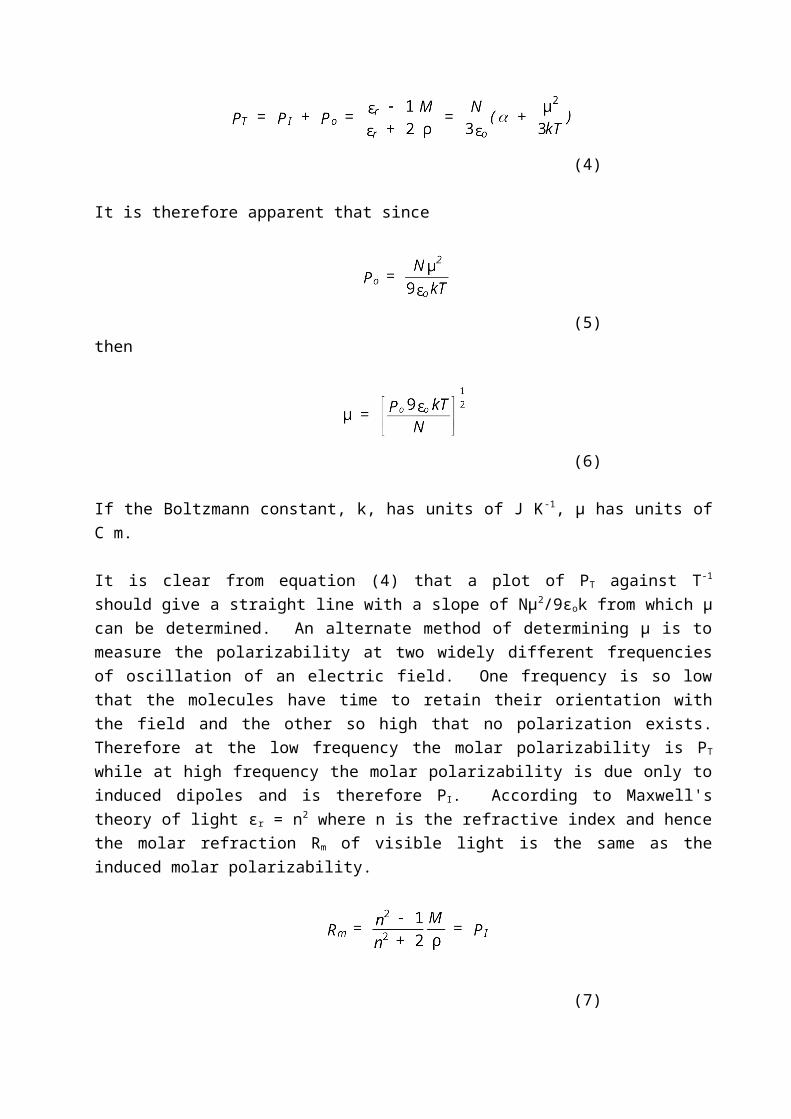
EXPERIMENT 11

DISSOCIATION CONSTANT OF ACETIC ACID FROMMEASUREMENTS OF ELECTRICAL CONDUCTIVITY

References: Atkins and de Paula, pp. 761-764.James and Prichard, pp. 239-243.

Definition of Terms:Resistance (R)If a potential difference, V, is applied between two points in a conductor, and an electric current, i, flows through the conductor, the electrical resistance is defined as R = V/i.Units: ohm,

Conductance (G)The conductance is defined as the reciprocal of resistance, i.e. G = l/R.Units: siemens, S

Resistivity ()The resistivity () of a material is the resistance of a cube of the material with sides of unit length. The resistance is directly proportional to the length of the sample and inversely proportional to the cross-sectional area and so it would be incorrect to refer merely to unit length of the material in the above definition.Units: m

Conductivity ( ) The conductivity is defined as the reciprocal of resistivity, i.e. = l/.Units: S m1.

Molar Conductivity ( m)The molar conductivity is defined as the current carried by one mole of an electrolyte under unit potential gradient. The relationship between m and is

where c is the concentration which must be expressed in mol m 3 in order to obtain values of m in units of S m2 mol1. The molar conductivity is a measure of the current-carrying ability of an electrolyte. For example, a 1 mol dm -3 HCl solution has a higher molar conductivity than a 1 mol dm-3 NaCl solution. This is because the H+ ion is a better conductor of electricity than the Na+ ion.

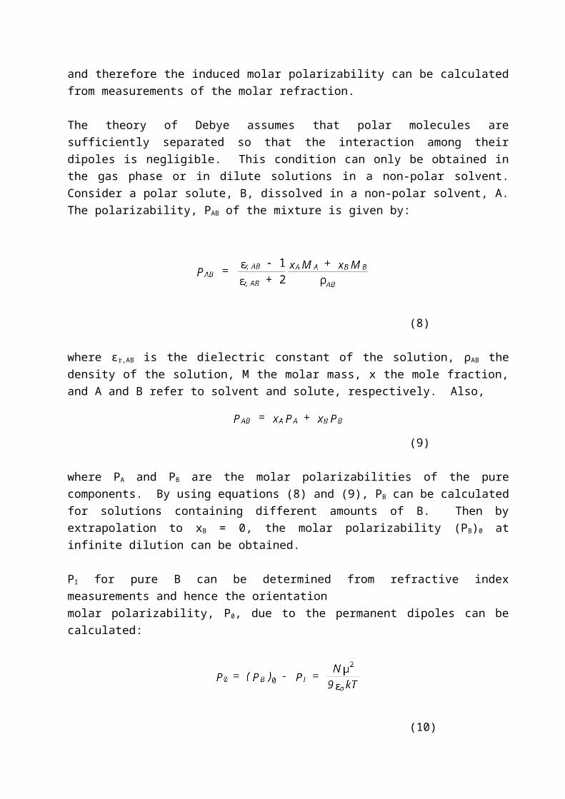
Equivalent Conductivity ( eq)For the electrolyte Mv+X yielding the ions M2+ and X2 in solution, the equivalent conductivity is defined as

Thus

The equivalent conductivity is a measure of the current-carrying ability of an electrolyte per faraday of positive (or negative) charge produced on dissociation.

Two types of instrument are available for measuring conductivity; those which measure conductance or resistance, and those which measure conductivity directly.

A conductivity cell is used to determine the conductance of the solution. This consists of two flat platinum electrodes which are coated with platinum black and are rigidly fixed in place so that their positions relative to one another remain fixed. The rest of the cell is made of glass and, when the cell is dipped into a solution, the electrodes are completely covered by the solution. The determination of the conductivity of the solution now involves the measurement of the resistance of the solution between the electrodes.

The apparatus used is basically a Wheatstone bridge arrangement. An A.C. supply must be used to avoid polarisation and consequent ‘back electromotive force’. The supply to the bridge should be an audio-frequency signal. The conductivity bridge is adjusted so that a point corresponding to maximum deflection of the detector is obtained. The resistance (or conductance) is then read off directly on the instrument.

The conductivity of the solution is related to the resistance measured, by the equation = l/AR where R is the resistance, l the distance between the electrodes and A the area of the electrodes. This can be written = G where is called the cell constant since it depends on the dimensions of each individual cell. The cell constant must then be known before a measurement of the conductance of a solution can be converted into the conductivity of the solution. The cell constant is determined by measuring the conductance of a solution for which the conductivity is known. Typically a solution of KCl is used.

You will use an instrument that is designed for the direct measurement of conductivity. In this case it is not necessary to determine the cell constant of the conductivity cell, as described above. The cell constant of the conductivity cell is determined by the manufacturer and is engraved on the outside of the cell. The user is required to calibrate the instrument by ensuring that the value of the cell constant supplied by the manufacturer is entered into the instrument when the latter is in calibration mode. The instrument may

subsequently be used for direct measurement of solution conductivity. Note that although the mode of operation of this type of instrument differs from those that measure conductance or resistance, the essence of the instruments (Wheatstone bridges with A.C. supply) are all the same.

When an instrument such as this one which purports to provide a direct measurement of the desired quantity, in this instance a conductivity, is used, it is a wise precaution to test the system by measuring the conductivity of a solution whose conductivity is accurately known. For this purpose, a solution of about 0.1 mol dm3 KCl is made up, the exact amount of KCl used being known. The molar conductivity (and hence the conductivity) of the solution is then calculated from the equation:

This calculated value may then be compared with the conductivity value obtained experimentally by use of the conductivity meter. Any significant discrepancy should be reported.

The Dissociation Constant of Acetic Acid:Weak electrolytes do not dissociate completely in solution except at infinite dilution. An approximation to the fraction of molecules which do dissociate, called the degree of dissociation, , at a concentration c is given by

where m,c and m,0 represent the molar conductivities of the electrolyte at concentration c and at infinite dilution, respectively. m,0 for any electrolyte (weak or strong) may be obtained from the appropriate published tables.

Consider the dissociation of a weak acid of overall concentration c mol dm 3, and the moles present at equilibrium in 1 dm3 of solution:

HA H+ + A

c(1 ) c c

We then have

Ka is called the dissociation constant.

Substituting for we get

Thus Ka can be obtained from conductivity measurements.

Note:(i) The equation = m,c/m,0 is only approximate because it does not take into account

the forces of attraction and repulsion exerted by ions on one another at finite concentrations.

(ii) If is small we can write

or

This shows clearly that as the dilution increases the degree of ionisation increases.

Experimental Procedure:Make up solutions of 0.02 mol dm-3, 0.002 mol dm-3 and 0.0002 mol dm-3 acetic acid from the 0.1 mol dm-3 acid. This is most conveniently done by successive dilution. Determine the conductivity and hence the molar conductivity of these solutions, including the 0.1 mol dm -3

solution, at 25 C. The conductivity of the water should be subtracted in the case of the more dilute solutions.

Calculate the degree of dissociation and dissociation constant in each case. The latter should be approximately constant. The electrodes must be well washed and dried externally after each determination.

Note:(i) Use of a thermostat is important in all the above experiments as conductivity varies

with temperature (about 2% per degree). Solutions should be left for 15 minutes in

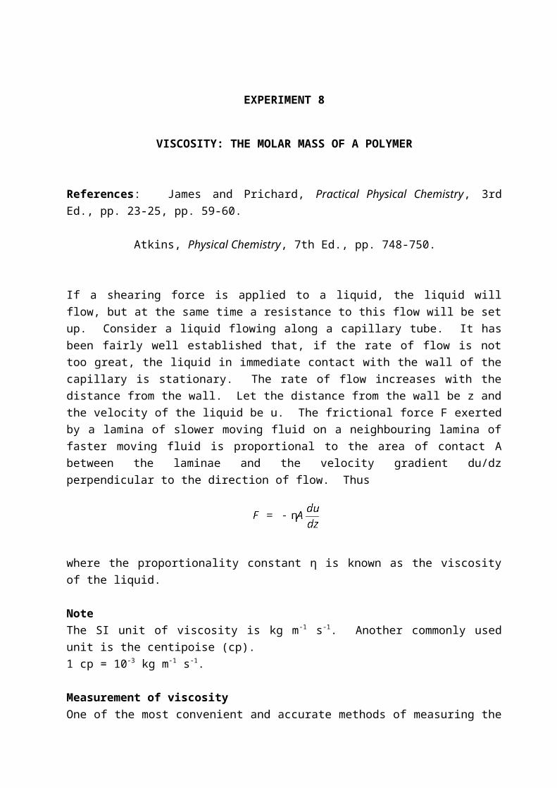
the thermostat bath before measurements are made.

(ii) The water used in all conductivity experiments must be exceptionally pure, i.e. it must have a very low conductivity, not greater than 1 x 104 S m1. Water of this quality can now be readily obtained using ion exchange resins and is called conductivity water. The conductivity of the water used should be determined. For best results, the conductivity water coming directly out of the resin column should be used, rather than water that has been standing in the reservoir for some time.

(iii) A published value for the dissociation constant of acetic acid may be found in most textbooks on analytical chemistry.

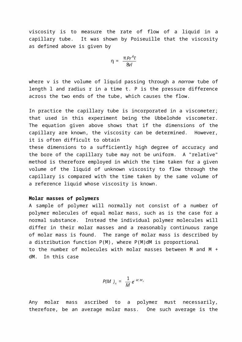
Experiment 12

THE RATE OF HYDROLYSIS OR ‘INVERSION’ OF SUCROSE,BY POLARIMETRY

References: Atkins and de Paula, pp. 791-803.James and Prichard, pp. 88-89 and 199-200.

Introduction:First-Order ReactionsThe hydrolysis of sucrose occurring in aqueous solution can be written as the reaction

C12H22O11 + H2O C6H12O6 + C6H12O6

sucrose D-glucose D-fructose

which proceeds virtually to completion. Kinetic data indicate that the reaction has a rate law

.....(1)

where v 6. However, since one of the reactants, water, is present in great excess, [H 2O] remains effectively constant during the course of the reaction. Also, [H+] remains constant during a particular reaction run, so the rate law becomes, effectively

.....(2)

where k = k[H+][H2O]v. The reaction is therefore an example of a pseudo-first order reaction.

The rate law (2) can be re-written as follows:

.....(3)

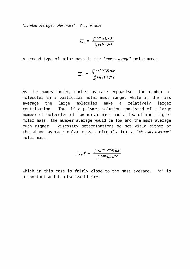
Equations (2) and (3) are valid at any stage during the reaction. Equation (3) can be integrated from the start of the reaction, i.e. from t = 0, [C 12H22O11] = [C12H22O11]0, to any time t later, when the concentration of sucrose is denoted [C12H22O11].

.....(4)

Equation (4) is the integrated form of equation (2) and shows that the concentration of sucrose in solution should decrease exponentially with time from an initial value of [C12H22O11]0 to a final value of zero as t .

Optical ActivityPlane polarized light can be produced in a number of ways, including(i) transmission of unpolarized light through a sheet of a commercial polarizing material

called polaroid;

(ii) reflection of unpolarized light from a planar reflective surface orientated at a certain angle of incidence with respect to the incident light;

(iii) transmission of unpolarized light through a suitably cut doubly-refracting crystal, e.g. calcite.

It is also possible, by appropriate use of doubly-refracting crystals (usually thin sheets of mica), to produce what is known as circularly polarized light. Circularly polarized light is light in which the plane of the electric field (and therefore also the plane of the magnetic field) rotates as the light beam advances. If the plane of the electric field rotates clockwise as observed facing the light source, the light is said to be right circularly polarized light. If it rotates counterclockwise, it is left circularly polarized light. When left and right circularly

polarized beams of equal intensity are combined, they yield plane polarized light. Conversely, a beam of plane polarized light can be regarded as a superposition of two beams of circularly polarized light of equal intensity but rotating in opposite senses.

It is an observed fact that certain solid crystals, and also certain liquids and solutions, have the ability to rotate the plane of polarization of plane-polarized light. Such materials are said to be optically active. Optically active substances show different refractive indices when refractive index is measured using left- and right-circularly polarized light, respectively. This implies that left- and right-circularly polarized light travel at different velocities through an optically active medium. It follows, therefore, that when a beam of plane polarized light has passed through an optically active medium, the left- and right-circularly polarized component beams will emerge from the medium out of phase with one another.

The result will be a change in the orientation of the resultant plane of the electric field of the radiation, as indicated in the diagram above.

A liquid or a solution shows optical activity when it contains molecules which are dissymmetric or chiral. A molecule is said to be dissymmetric or chiral when the molecule and its mirror image are non-superimposable. A simple example of a chiral molecule is lactic

acid.

The substances dealt with in this experiment, sucrose, D-glucose and D-fructose, all consist of chiral molecules, and are therefore optically active.

Optical RotationWhen plane polarized light passes through an optically active medium, the plane of polarisation of the light is rotated through an angle which is denoted α and is termed the ‘angle of optical rotation’. The quantity α can be expressed in degrees (°) (as read off the polarimeter scale) or, preferably, in radians (rad).

In order to characterise the optical rotatory power of particular substances, the following quantities have been used:

(1) The ‘specific optical rotatory power’, given by

where V represents the volume of solution in the polarimeter tube; m the mass of the optically active subtance in the tube; l the length of the tube; and c the mass concentration of the optically active substance. The SI unit for αm is rad m2 kg1.

(2) The ‘molar optical rotatory power’, given by

where α, V and l are as defined previously; n represents the amount of optically

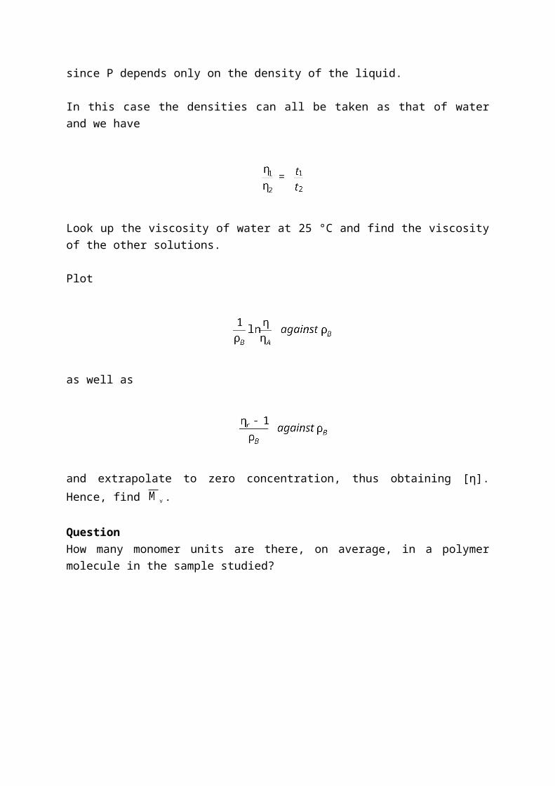
active substance (mol) in the tube; and c the concentration of the optically active substance. The SI unit for αn is rad m2 mol1.

It can be shown that, in this experiment, [sucrose] α (αt - α).

Experimental Procedure:1. Dissolve 50 g of sucrose in water and make up to a final volume of 250 cm3. The

resulting solution contains 0.2 g of sucrose per cm3 or 20% sucrose by mass.

2. Take 40 cm3 of the above solution and dilute to 100 cm3. Determine the zero reading of the polarimeter with water in the polarimeter tube and determine the angle of optical rotation, αo, of the light for the 8% sucrose solution. Calculate the specific optical rotatory power of sucrose.

3. Dilute 40 cm3 of the 20% sucrose solution to 100 cm3 by using 2 mol dm-3

hydrochloric acid and start the clock. Wash the polarimeter tube twice with this (reacting) sucrose-acid solution. Then fill the tube and follow the angle of optical rotation, αt, as a function of time. Note the angle of optical rotation, αt, and time, t, every 15 minutes.

4. Determine α, the angle of optical rotation corresponding to the mixture at the end of the reaction, by heating the remaining sucrose-acid mixture for about 30 minutes at 60 to 70 °C.

5. Determine the rate constant k, from a plot of ln{(αt - α)/rad} against time/s. The units of k are s1. Specify the temperature for which this rate constant is valid.

Notes:1. Consult a demonstrator in connection with the correct procedure for setting the zero

on the polarimeter, and the procedure for measuring angles of optical rotation.

2. Since the rate and the rate constant of a chemical reaction are strongly temperature dependent, make sure that the reaction takes place at room temperature. Record the temperature.

3. Fill the polarimeter tubes by using a pipette. Dry the tube carefully before inserting into the polarimeter. Make sure that no air bubbles are present in the tube.

4. Since solid sucrose is rather hygroscopic, close the reagent bottle after use.

5. Clean the polarimeter tube after use by rinsing it three times with distilled water. Dry the tube on the outside.

Questions:1. What is the role of H+ in this reaction? What is the value of [H+] at the start of the

reaction? Can this value change as the reaction proceeds?

2. Why is ln(αt - α) plotted against t instead of, say, ln αt against t?

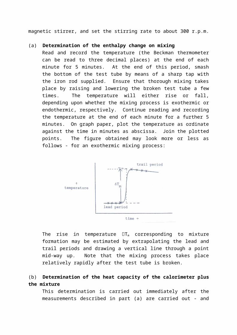
EXPERIMENT 13

A COMPLEX REACTION – THE BROMINATION OF ACETONE

Reference: F. Daniels, J.W. Williams, P. Bender, R.A. Alberty, C.D. Cornwall, J.E. Harriman, Experimental Physical Chemistry, 7th edition, pp. 152-155.

Introduction:The purpose of this experiment is to determine the rate law and the rate constant for the bromination of acetone. From rate data collected at two or more temperatures the activation energy is estimated.

The bromination of acetone in acid solution proceeds according to the reaction equation

(1)

The reaction is catalyzed by hydrogen ion. The rate law is assumed to be of the form

(2)

where k is the rate constant and [A] represents the concentration of A in moles dm -3. The exponents p, q and r indicate the order of the reaction with respect to acetone, bromine, and hydrogen ion, respectively.

The bromination of acetone is a particularly convenient and interesting reaction to study kinetically. The progress of reaction is readily followed by directly observing the decrease in bromine concentration spectrophotometrically at a wavelength where none of the other reagents has significant absorption. Further, the reaction provides a remarkable demonstration of the general rule that it is not possible to predict the rate law from just the knowledge of the stoichiometric equation. As will be confirmed in this experiment, the reaction is zero order in bromine, that is, q in equation (2) is zero. This result provides a straightforward application of the method of initial rates wherein the acetone and acid are present in large excess while the bromine is used in small concentrations to limit the extent of reaction. The small amount of bromine is completely consumed while the other reactants remain at an essentially constant concentration. Since the reaction velocity is independent of the bromine concentration the velocity is constant until all of the bromine is consumed. Under these conditions

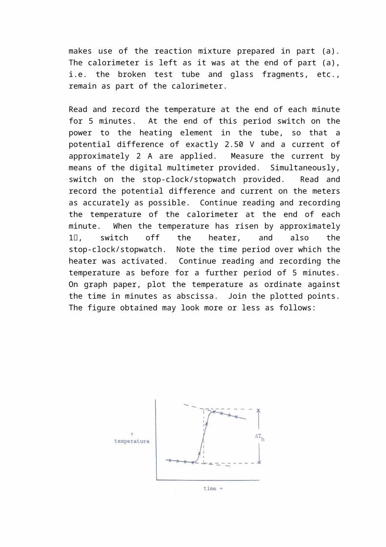
(3)

and therefore a plot of [Br2] against time is a straight line whose slope is the reaction rate.

For the determination of the exponent p it is necessary that the reaction be followed in two runs in which the initial concentrations of acetone are different while the initial concentrations of hydrogen ion are not changed from one run to the next. Using superscripts I and II to denote the two experiments, we have [CH3COCH3]II is say u times [CH3COCH3]I and [H+]II = [H+]I. Then from equation (3) we have

(4)which yields

log (rateII/rateI) = p log(u) (5)

or

(6)

The exponent r is determined from two runs, say I and III, in which [CH 3COCH3]I = [CH3COCH3]III and [H+]III = w[H+]I. These conditions lead to

(7)

The rate constant is then determined according to equation (2) from the exponents, reaction rate, and the concentration data for which the rate applies.

The activation energy Ea may be estimated from the Arrhenius relationship

k α exp(−Ea/RT) (8)

if the rate constant is known at two or more temperatures. The empirical rate law is

assumed to hold at the other temperatures so that one needs only to measure the rate for a set of known concentrations at each temperature of interest.

The bromine concentrations are determined from measurements of the absorption of blue light by the solutions. The absorbance is given by

A = єbc (9)

where є is the molar absorptivity, b is the sample path length in centimeters, and c is concentration in moles per dm3. For bromine dissolved in distilled water є is 160 mol dm -3

cm-1 at 400 nm. The absorbance should be in the range of 0.7 to 0.2 for greatest accuracy. Since cuvettes commonly have a sample path length of 1 cm, the desired concentration range for bromine in the reaction mixture is from 0.0044 mol dm -3 to 0.0012 mol dm-3. For cuvettes which have been selected for close optical matching and close matching of path length, the constant є and b of equation (9) may be taken together as a constant B to give

A = Bc (10)

It is recommended that the constant B be determined experimentally.

Experimental Procedure:

CAUTION: Experimental operations involving bromine should be carried out in a fume cupboard and solutions containing bromoacetone should be kept stoppered.

All absorbance measurements are to be made at 400 nm.

The constant B of equation (10) is determined by measuring the absorbance of three solutions of known bromine concentration. Prepare one solution by pipetting 10.0 cm3 of stock 0.02 mol dm-3 Br2 into a clean 50 cm3 Erlenmeyer flask. Add 10.0 cm3 of 1 mol dm-3 HCl and fill to the mark with distilled water. Mix the solution thoroughly and measure the absorbance. Repeat this procedure by using first 6.0 cm3 and then 3.0 cm3 of 0.02 mol dm-3

Br2 diluted in each case with 10.0 cm3 of 1 mol dm-3 HCl and sufficient distilled water to give a total volume of 50.0 cm3 of solution. Record the three values of absorbance and concentration.

The reaction rate is to be measured at room temperature for four different solutions. The appropriate quantities of acetone and hydrochloric acid are first mixed together in a 50 cm3

volumetric flask. The clock is started when the proper amount of bromine water is added to the flask. Stir the reaction mixture thoroughly and quickly. Rinse a clean cuvette with the reaction mixture, fill it and place it in the spectrophotometer. Record the absorbance and the time about every minute until ten to twelve readings are obtained or until the

absorbance falls below about 0.1. Record the temperature of the solutions. Satisfactory reaction solutions are prepared as shown in the Table. For each solution add distilled water to make a total volume of 50 cm3.

TABLE

Solution Number

0.02 mol dm-3 bromine/cm3 4.0 mol dm-3 acetone/cm3 1.0 mol dm-3 HCl/cm3

1 10 10 10 2 10 5 103 10 10 54 20 10 10

Early in the laboratory period place some of each of the stock solutions and distilled water in the constant temperature bath at the desired higher temperature (30 ºC to 35 ºC is suitable) and allow sufficient time for them to reach thermal equilibrium. The proper quantities of acetone, hydrochloric acid, and distilled water may be mixed before placing them in the constant temperature bath. Both of the reaction mixture number 2 and 3 may be used at the higher temperature. Mix the solutions and record absorbance and time as was done for the solutions at room temperature. Record the temperature of the solutions just before mixing.

Calculations:From the absorbance measurements on the three solutions of bromine water determine an average value of B in equation (10). Use this result to compute the concentration of bromine for each absorbance reading in the kinetic runs. For each run prepare a plot of [Br 2] against time and determine the rate = ∆[Br2]/∆t. Equations (6) and (7) are used to compute the order of reaction with respect to acetone and with respect to hydrogen ion. An analogous equation is used along with the data on solutions number 1 and 4 to calculate the order with respect to bromine.

Use equation (3) and the experimental results obtained to calculate the rate constant k for each of the kinetic runs. Determine an average value of k for each temperature used in the experiment. If the reaction is studied at only two temperatures the activation energy may be estimated from

If more than two temperatures are studied plot log k against 1/T. The slope = −E a/2.303R

yields the activation energy.

Experiment 14

DISSOCIATION CONSTANT OF AN INDICATORBY SPECTROPHOTOMETRY

References: James and Prichard, pp. 93-97.

Experimental Procedure:Consult the demonstrator about the operation of the spectrophotometer.

You are provided with a stock solution of the indicator, methyl red (0.1 g per 250 cm3).Prepare, accurately, the following solutions:

(a) 1 cm3 indicator made up to 50 cm3 with 0.01 mol dm-3 HCl

(b) 1 cm3 indicator made up to 50 cm3 with 0.01 mol dm-3 NaOH

(c) 1 cm3 indicator made up to 50 cm3 with pH 4.0 buffer

(d) 1 cm3 indicator made up to 50 cm3 with pH 5.0 buffer.

Plot the absorption curves of these four solutions over the region 400 to 600 nm at 10 nm intervals. The four curves should intersect at one point, the isobestic point. (Measure the pH of all four solutions with the pH meter provided.)

Confirm the Beer-Lambert law by determining the absorbance of one of the solutions at a fixed wavelength, at say four different concentrations (e.g. by diluting one of the above solutions, listed in (a) (d), successively 1:1 with 0.01 mol dm -3 HCl, 0.01 mol dm-3 NaOH or the buffer solutions as appropriate).

Note:(i) Once a cell is filled with solution, it should be carefully wiped with tissue-paper to ensure

that the transparent sides of the cell are completely clean, i.e. free from any traces of liquid or fingerprint marks. There should also be no air bubbles in the path of the light beam.

(ii) At each change of wavelength, the instrument should be re-zeroed.

(iii) The pH meter should be calibrated using the two standard buffer solutions provided.

Calculation:Absorption of light by a solution is governed by the Beer-Lambert law:

where is the molar absorptivity, c the concentration of the solution in mol dm3, l the length of the absorption cell in cm, Io the intensity of the incident radiation and I the intensity of the radiation after passing through the cell.

The absorbance, A, is given by A = log (Io/I).

The dissociation of a weak acid of concentration c can be represented by

HA H+ + A.

Assuming that the absorbances of the two forms of the indicator are additive we have

cmix = cHAHA + cAA ;

alsoc = cHA + cA.

From these two equations we get

also

i.e.

or

Thus pKa can be calculated.

Hint: It can be assumed that at pH 2 all the indicator will be in the protonated form (HA), and that at pH 12, all the indicator will be in the deprotonated form (A).

Questions:1. Why should all four spectra intersect at a single point, i.e. the isosbestic point? If they

do not all intersect at a common point, what would this indicate?

2. In the test of the Beer-Lambert law, would it have been correct to dilute the solutions with water? If not, why not?

3. For calculating the pKa of the indicator, should use be made of absorbance data obtained at wavelengths at, or close to, the isosbestic point? If not, why not?

Experiment 15

DIFFERENTIAL SCANNING CALORIMETRY (DSC)

OBJECTIVES This experiment has the following three objectives:

1. to observe the phase transitions crystalline nematic and nematic isotropic liquid for a nematic liquid crystal 4,4'-di-n-hexyloxyazoxybenzene and

2. to determine for the melting of indium metal Tfus, Hfus and Sfus. 3. to operate a precision differential scanning calorimeter (Perkin-Elmer DSC7) with

appropriate samples.

BACKGROUND

Matter upon the absorption of heat can channel the heat into raising the temperature of the sample under study or causing a structural change such as a phase transition. A structural change could be endoergic, i.e. heat is absorbed from the surroundings, or exoergic, i.e. heat is given off to the surroundings. One instrument that has the capability of quantitatively measuring the heats involved as a function of temperature or time (since a constant heating rate is used) is the Differential Scanning Calorimeter (DSC). The key idea involved in this instrument is that two compartments, sample and reference, are purposely maintained at a very small temperature difference of ±0.01°C. Each compartment has two heaters - a main heater and an auxiliary heater. An experiment is started by supplying power to the main heaters so that the temperature of each compartment begins to rise. Very small differences in temperature between the two compartments will result in practice. There is a thermopile (set of thermocouples) between the reference and the sample cells, which senses the off-balance temperature T and produces a corresponding voltage. This small voltage (0-5µV) is amplified by an operational amplifier. The amplified voltage is used to drive the auxiliary heater on the sample cell, which then acts to keep the off-balance signal close to zero. The instrument displays the differential power, P, between the two cells as a function of temperature of the heating compartments or furnaces as shown in Figure 1.

Figure 1: Differential power P vs. temperature T of a sample.

The temperature is determined by the thermopiles. The area under the peak of power versus temperature (temperature is related to time since the heating rate is constant) will give energy which is the enthalpy change H

(1)

The DSC reports the enthalpy per gram . Therefore to determine the molar enthalpy

change ,

(2)

where M is the molecular weight of the sample and m is the mass of the sample.

PROPAGATION OF ERRORS FOR

The propagation of errors for this experiment has some subtleties. For this reason a separate discussion on the determination of the 95% confidence limit for H is presented. The software of the DSC instrument gives a value of H/m in units of J g-1. The 95% confidence limit of H/m can be determined as tN s / N by repeating the experiment N times with the

same mass and the same heating rate. Now to determine we first define I as the integral that appears in equation (1); then

(3)

The uncertainty in I is not provided by the software but can be determined from

(4)

to be

(5)

further, we assume dT/dt is negligible here. We can then determine from

(6)

that

(7)

from which can be determined.

PROCEDURE Before beginning a few points are worth noting. Sample weighings are carried out using a microgram balance with an uncertainty no greater than a few hundredths of a mg--take the uncertainty to be ±0.010 mg. Also, in running software with the Perkin-Elmer DSC7 tasks will be accomplished through using function keys F1-F9.

A. DSC Run with 4,4'-di-n-hexyloxyazoxybenzene 1. First make three (3) weighings of a pan and a cover. Use the 95% confidence

limit m determined here to apply to all other weighings. Next weigh a sample, about 10 mg, of the liquid crystalline solid in the pan. Place a sample cover on top of the sample and crimp the edges of the pan. The lab instructor will demonstrate the technique.

2. Turn on in this order: a. the DSC7 instrument and then b. the instrument controller PC.

A main menu will appear. Select the Multi-tasking menu to set the operating Parameters and Conditions as follows for the liquid crystalline material and press ENTER. Next, press F1 (Go To Setup) and at the next screen select F1 (Parameters). The following information should appear on the screen and the values shown should be entered:

Parameters (other values default)

Final Temp. 90°C

Start Temp. 65°C

Scanning Rate 2.5°C/min

Sample Weight your value of mass of liquid crystal in mg

then press ESC. Press F2 (Conditions) and the following information should appear on the screen and the value shown should be entered.

Conditions (other values default)

End Condition H (means "Hold")

Load Temp. 50°C

Go to Temp. Rate 200.0°C/min

Y Initial Value 20.0 mW3. Place the empty sample pan + cover on the right-hand side table (reference) and

the crimped sample pan on the left-hand side table of the DSC7. Place a platinum cover over each table. In handling pans and covers use forceps. Close the head of the DSC7. Press F3, Id sample, and enter a suitable label.

4. Under F5 (Direct Control) use the F1 key to go to the Start Temperature desired for this run. After the system has reached the Start Temperature, note the power given near the top left-hand part of the screen. Once this value has stabilized set the Y Initial Value under Conditions to this value.

5. Begin the DSC run by pressing F6 (Begin Run). Very soon thereafter, the sample identity label and the power difference will blink on the screen and the trace of the data will be displayed on the screen as the run progresses. Let the system proceed to the planned end of the run UNLESS there is reason to interrupt operation by pressing F1 (which should now be labeled Stop Run). The Setup main menu should reappear after the run is complete.

6. Press F9 (Analysis) and choose F1 (Peak). Using the key, move the dashed vertical line to the left side of the peak. Press Home and use the key to move the other dashed vertical line to the right side of the peak. Then press the Enter key. BE SURE TO SAVE YOUR DATA TO A FILE.

7. After the plot of P vs T appears on the screen, press ESC, then F5 (Print Options); follow this by F1 (Print Screen)--be sure to select enhanced in the options.

8. Do 3 similar scans (steps 2 - 7 above) BUT NOW with: a. Final Temp = 140 and Start Temp = 115 b. Final Temp = 115 and Start Temp = 140 c. Final Temp = 60 and Start Temp = 90

BE SURE TO SAVE YOUR DATA TO FILES AND GENERATE PRINTOUTS FOR EACH RUN.

B. DSC run with indium metal 1. Similarly weigh a sample, about 10 mg, of In metal in an aluminum sample pan.

Again place a sample cover on top of the sample and crimp the edges of the pan.

2. Choose F5 (Direct Control) and F2 (Go to Load). Set up for a new run: Final Temp. 165°C

Start Temp. 150°C

Sample Weight (your value of mass of In sample in mg)

3. Replace the sample pan containing the liquid crystalline sample with the In sample pan prepared earlier. Carry out a similar run as in steps (2-7) above, and obtain a printout.

4. Do the reverse run as in step 2 by selecting the following settings under Parameters:

Final Temp. 150°C

Start Temp. 165°C5. Again save your data to a file and obtain a printout.

C. Transition Temperatures for 4,4'-di-n-hexyloxyazoxybenzene 1. Take a small amount of the liquid crystalline material and place it between two

microscope slides.

2. Use a polarizing microscope and determine the crystal(c) nematic(n) transition temperature and the nematic(c) isotropic liquid(i) transition temperature. Take polaroid pictures at each phase transition.

CALCULATIONS

1. Comment on any contrast between the behavior in the scan up and scan down runs with each sample.

2. Calculate (in J mol-1) for each process identifiable from the differential scanning calorimetry runs made. Look up, with reference(s) cited, corresponding values reported in the literature. Also look up values of Hfus for Hg, Na, and Pt and one other metal of your choice. Note and record melting temperatures for these same metals.

3. Compare the transition temperatures of the liquid crystalline sample with the transition temperatures estimated from the DSC runs.

4. For the liquid crystalline solid determine S (in J K-1 mol-1) for each phase transition. Why should there be a large difference in S for the 2 phase transitions: s n and n i?

5. For the In sample, calculate Sfus (in J K-1 mol-1) for In and for each metal involved in #2 above. Comment on any regularity (known as Richards' rule), the analog of Trouton's rule for the s l transition for metals.

REFERENCES

1. Atkins, P. W.; "Physical Chemistry," 5th ed., Freeman (1994) pp. 134-136; Tables. 2. Arnold, H., Z. Phys. Chem. (Leipzig) 226, 146, 1964. 3. Brown, G. H.; Doane, J. W.; Neff, V. D., "A Review of the Structure and Physical

Properties of Liquid Crystals," CRC Press (1971), pp. 39-43. 4. Demus, C; Fietkau, C. H.; Schubert, R.; Kehlen, H., Mol. Cryst. Liq. Cryst. 25, 215, 1974. 5. Cox, R. J.; Johnson, J. F.; IBM J. Res. Dev. 22, 51-59, 1978.

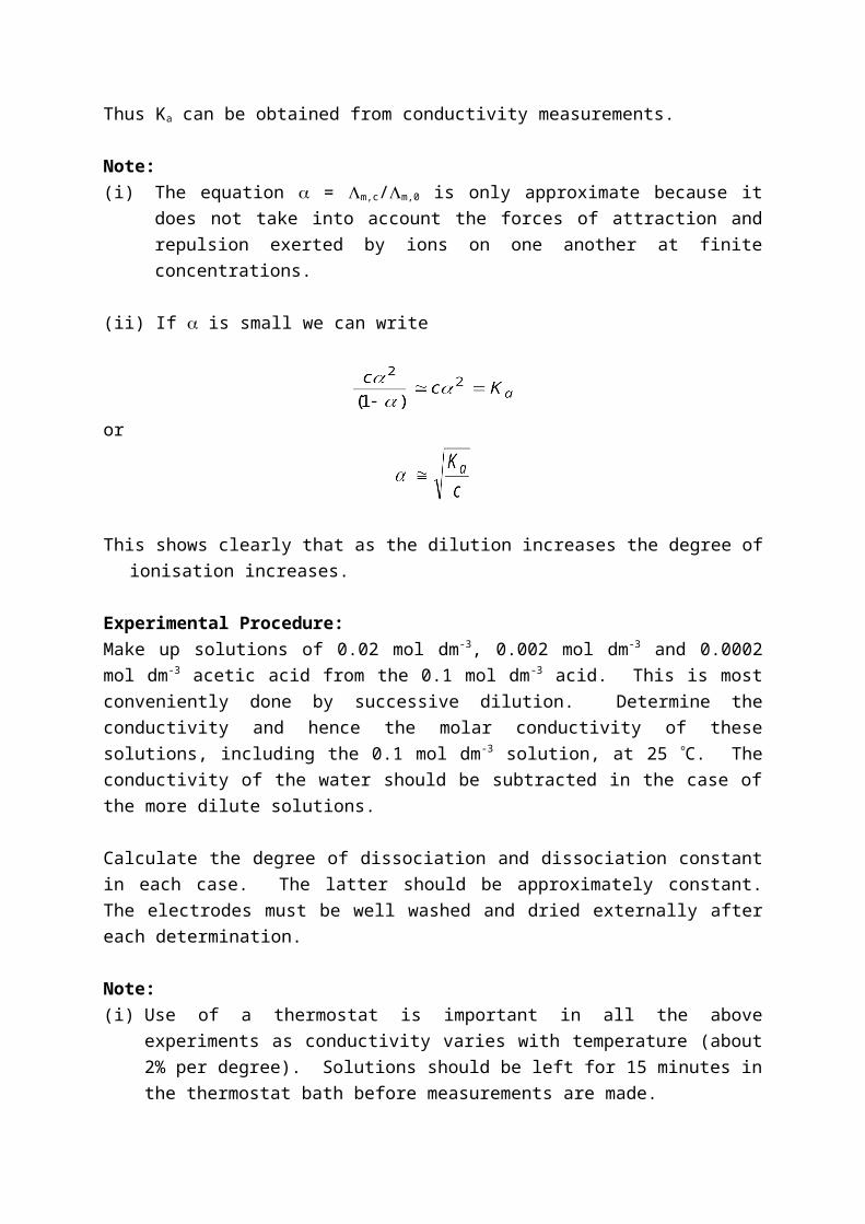
6. (a) Gruger, A.; Romain, F.; Le Calve, N.; Mol. Cryst. Liq. Cryst. 116, 57-84, 1984. (b) ibid, 116, 85-109, 1984.

EXPERIMENT 16

Chemical Oscillations and Waves: The Belousov-Zhabotinskii Reaction.

The study of oscillating chemical reactions and other systems that exhibit exotic dynamics has

been a very active area of research since the work by de Kepper et al, in 1981 which proved

that such exotic behavior can be designed and modeled. The previously known systems were

all discovered by accident. The idea of chemical oscillatory behavior had several detractors

who felt that such behavior violated the well known second law of thermodynamics which

implies that all physico-chemical systems proceed to positions of lowest free energy.

The Belousov-Zhabotinskii (BZ) reaction involves the oxidation of an ionizable organic

substrate (typically malonic acid) by acidic bromate while being catalyzed by weak one-electron

metal ion oxidant. Some of the metal ion catalysts include Ce3+, Mn3+, Fe2+ and Ru2+ complexes.

Apart from malonic acid, other organic substrates used include citric acid, bromomalonic acid,

and malic acid.

When oscillating reactions were first reported, many thought that these oscillations

were an artifact of heterogenous phenomena such as bubble formation, cavitation, or due to

the influence of dust particles. Of course, there was even more strenuous and vigorous denial

of the spontaneous formation of patterns which have been observed in the BZ reaction. A

possible explanation for the seeming violation of the second law of thermodynamics presented

by the oscillatory nature of the BZ reaction was offered by Ilya Prigogine. His explanation as

well as his theories on the thermodynamics of systems far from equilibrium landed him the

1969 Nobel Prize in Chemistry. Prigogine’s reasoning was that a system could organize

(decrease its entropy) as long as the net entropy change of the universe was positive. Thus the

concentrations of intermediates in a reaction can oscillate while the free energy monotonically

decreases. The decrease in entropy caused by the periodic concentration changes is more than

compensated by the entropy increases from other processes also concomitantly proceed in the

reaction mixture. Hence a system already at equilibrium is unlikely to show any oscillatory

behavior because the total entropy has already attained its maximum value. Any oscillatory

behavior at this stage will be equivalent to a perpetual motion machine and this definitely

violates the inviolable second law of thermodynamics.

In the human body, spontaneous formation of proteins occurs even though the ΔG of

formation of the peptide bond is positive. Protein synthesis, however, still proceeds because it

is coupled to other reactions whose free energy changes are negative, yielding an overall net

decrease in free energy.

Ever since the study of chemical dynamics began, the BZ reaction has proved to be the

most fascinating reaction ever studied. Many research groups spend their lives studying this

reaction and never fully exhaust its capabilities. While it is well known to be oscillatory, one of

its other features is excitability. In the excitability mode, the BZ reaction is not oscillatory, but

will remain is some quasi-steady state until perturbed. The perturbation will cause the BZ

system to undergo one full oscillation before returning to the original state. Such a system will

show transverse traveling waves of chemical reactivity due to the coupling of the diffusion with

the basic autocatalysis that characterizes the reaction’s kinetics. The types of patterns obtained

have shown a remarkable similarity to the patterns observed from aggregating slime molds.

This particular laboratory exercise will not deal with these spatial inhomogeneities, but strictly

with the oscillatory domain of the reaction.

Oscillatory Homogenous BZ Reaction

The basic object of this laboratory exercise is to study the behavior of the oscillatory BZ system.

Oscillations will be observed

(a) in the redox potential of the system, which is controlled by the ratio of the

concentrations of the reduced to the oxidized form of the metal ion catalyst;

[M(n+1)+]/[Mn+],

(b) the concentrations of the bromide ion, [Br-] and

(c) the colors, based on the concentrations of the colored metal ion complex. For

example, if cerium is used, the color will alternate between faint brown to colorless,

and if ferroin is used, the color will alternate between deep read and blue.

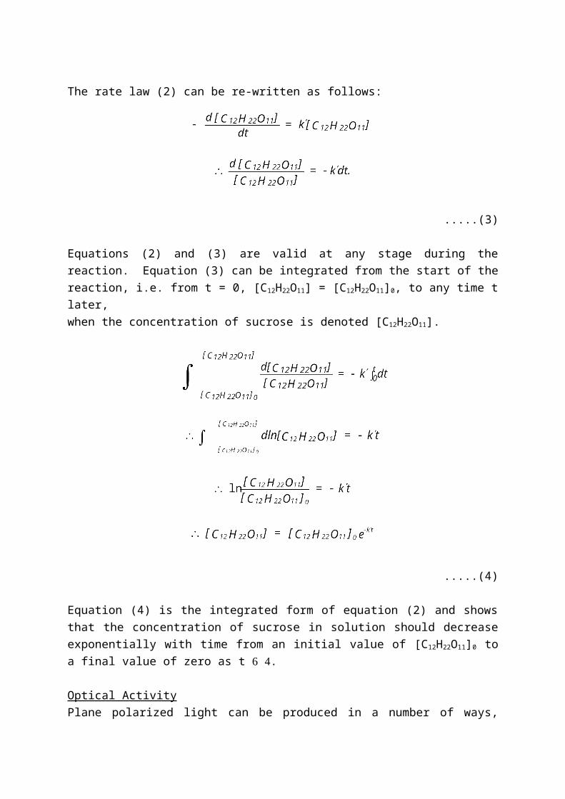
Assumed Mechanism of the BZ reaction.

The first accepted mechanism was by Richard Fields, Endre Koros and Richard Noyes at the

University of Oregon (see J. Am. Chem. Soc. Vol 94, 8649 – 8664, 1972). It is a complex,

rambling mechanism with over 21 proposed steps and 30 intermediates and products. An

analysis of the mechanism shows that it can be distilled to 9 important steps whose central

theme is the autocatalytic production of an intermediate, HBrO2. These reactions are

shown below as R1 – R6 and C1 – C3.

Table 1

Abbreviated FKN Mechanism for the BZ Reaction

(R1) Br− + HOBr + H+ → Br2 + H2O kR1 = 8× 109 M−2 s−1

(R2) HBrO2 + Br- + H+ → 2HOBr kR2 = 106 M−2 s−1

(R3) BrO−3 + Br- + 2H+ → HBrO2 + HOBr kR3 = 2.0 M−3 s−1

(R4) 2HBrO2 → BrO3- kR4 = 2× 103 M−1 s−1

(R5) BrO3- + HBrO2 + H+ → 2BrO2· + H2O kR5 = 10 M−2 s−1

(R6) BrO2 + Ce(III) + H+ → HBrO2 + Ce(IV) kR6 = 6× 105 M−2 s−1

(C1) CH2(COOH)2 (HO)2C = CHCOOH

(C2) (HO)2C = CHCOOH + Br2 → BrCH(COOH)2 + H+ + Br−

(C3) 2Ce(IV) + CH2(COOH)2 + BrCH(COOH)2 → fBr- + other products

Process A; Reactions R1 – R3

The overall stoichiometry of Process A is:

BrO3- + 5Br- + 6H+ 3Br2 + 3H2O (A)

This process reduces the concentration of bromide, but leaves the Ce(IV) concentrations

unaltered. Due to the excess of bromate concentrations used, [BrO3-] can be assumed to be

constant throughout the reaction. Some Br- is formed since Br2 reacts with the enolic form of

the malonic acid to form bromomalonic acid, BrMa.

Malonic Acid Enol (C1)

Enol + Br2 BrMa + H+ + Br- (C2)

Adding A + 3C1 + 3C2:

BrO3- + 2Br- + 3H+ + 3MA 3BrMa + 3H2O (H)

gives a net loss of only 2Br- per cycle in process A (instead of the expected 5Br-)

Process B becomes important when [Br-] becomes too low. This is when HBrO2 can

compete as reducing agent; Reaction R5. This forms Br2O4 which quickly splits into two BrO2.

BrO2 is a one-electron oxidant and can oxidize the metal ion by one electron (Ce(III) Ce(IV);

for example). See Reaction R6. R5 + 2R6 constitutes autocatalysis in HBrO2:

BrO3- + 2Ce(III) + HBrO2 + 3H+ 2HBrO2 + 2Ce(IV) + H2O (J)

The rate of this reaction rapidly accelerates and Ce(III) is changed autocatalytically to Ce(IV) in a

sigmoidal rapid upsurge. With tris(1, 10-phenathroline) Iron(II) as the redox catalyst, one

observes a dramatic color change from red (Iron(II) complex) to blue (Iron(III) complex. At this

point process A becomes less effective compared to process B. Process B is switched on when

[Br-] falls far enough for reaction R5 to effectively compete with R2. This gives a critical amount

of [Br-] for the switch over as:

[Br-]critical = 10-5 [BrO3-]0

When [Br-] > [Br-]critical; process A dominates, leading to a decrease in [Br-]. However, if it is the

other way round, the autocatalytic sequence of process B dominates, leading to an increase in

[Br-].

Experimental Procedure.

Weigh out carefully:

25 g of malonic acid

60 g sodium bromate

1.5 g tris(1,10-phenathroline) Iron (II) sulfate (ferroin)

Measure out, using a graduated cylinder, 24 mL concentrated sulfuric acid

1.02 g Sodium Bromide and dissolve this in 100 mL of water.

1.17 g Sodium Chloride and dissolve this in 100 mL of water.

Add the 24 mL of concentrated sulfuric acid to a beaker with 800 mL water (Not the other way

round!!!) and dissolve the sodium bromate in this solution. Call this Solution A.

Dissolve the malonic acid in a beaker with 250 mL of water. Call this Solution B.

Dissolve the ferroin in 100 mL of water. Call this Solution C.

The sodium bromide solution will be called Solution D

The sodium chloride solution will be called Solution E

Solutions A, B, and C will now constitute as your ‘stock solutions’. These are the ones we will

use to set up the oscillatory BZ system. The student should have enough for at least 5

experiments.

Place a large beaker on a magnetic stirrer supplied and mix the following while vigorously

stirring:

130 mL water

180 mL of solution A

30 mL of solution B

10 mL of solution C.

Add solution C last and set your stop watch. Record the time taken by the system to give the

first color change (call this ‘induction time’) and the time taken subsequently between color

changes. Follow the reaction 10 minutes.

Varying initial conditions:

Re-do the experiment but this time use 180 mL water and 130 mL of solution A while keeping

everything else the same and perform the same observations as above. What differences, if

any do you observe?

Now keep everything else the same, but use 140 mL water and 20 mL of solution B and make

the same observations.

Bromide Control:

Before adding solution C in the original BZ reaction mixture, add 2 mL of Solution D. From the

inferred mechanism, what would you expect with respect to the ‘induction period’? Is this your

observation? Do the periods change due to addition of solution D?

Chloride kills the oscillations?

After adding the full original BZ mixture, immediately add 2 mL of Solution E. What do you

observe?

Suggested Data presentation format:

Solution Time Period

Induction period T1 --

Change-1 T2 T2 – T1

Change-2 T3 T3 – T2

etc etc Tn – Tn-1