department for transport, energy & … · department for transport, energy & infrastructure...

DEPARTMENT FOR TRANSPORT, ENERGY & INFRASTRUCTURE HYDROLOGICAL STUDY OF THE FIRST TO FIFTH CREEK CATCHMENTS

TRANSPORT SERVICES 33-37 Warwick Street Walkerville, SA 5081 PO Box 1 Walkerville SA 5081

Telephone: 61 8 8343 2222 Facsimile: 61 8 8343 2585

id22669531 pdfMachine by Broadgun Software - a great PDF writer! - a great PDF creator! - http://www.pdfmachine.com http://www.broadgun.com

2

CONTENTS 1 INTRODUCTION....................................................................... 4 2 THE RRR MODEL..................................................................... 4 3 DEVELOPING THE RRR MODEL ............................................ 8 4 FITTING THE RRR MODELS ................................................... 8

4.1 Available Data...................................................................................... 8 4.2 First Creek � Waterfall Gully (AW504517) ........................................... 9 4.3 First Creek Downstream Botanic Gardens (AW504578).................... 10 4.4 Second Creek at Stepney (BM023104).............................................. 11 4.5 Third Creek at Forsyth Grove, Felixstow............................................ 13 4.6 Fifth Creek at Athelstone.................................................................... 13 4.7 Sixth Creek ........................................................................................ 14

5 FLOOD FREQUENCY ANALYSIS.......................................... 15 5.1 First Creek ......................................................................................... 15 5.2 Sixth Creek ........................................................................................ 19 5.3 Brown Hill Creek ................................................................................ 21

6 PARAMETERS FOR THE ESTIMATION OF DESIGN FLOWS 23

6.1 First Creek to Waterfall ...................................................................... 23 6.1.1 Comparison of Calibrated RRR Models and Flood Frequency Analysis 23 6.1.2 Derivation of Rural Design Losses.............................................. 25

6.2 Other Rural Catchments .................................................................... 26 6.3 August 2004 event ............................................................................. 32 6.4 Urban Catchments ............................................................................. 37

7 VERIFICATION OF RURAL PARAMETERS ON LARGE HISTORICAL EVENTS ................................................................. 38

7.1 June 1981 .......................................................................................... 38 7.2 March 1983 ........................................................................................ 39

8 PREDICTED HYDROGRAPHS 1:20 AEP to 1:100 AEP........ 41 9 THE SIGNIFICANCE OF HISTORICAL FLOOD EVENTS...... 44 10 PROBABLE MAXIMUM FLOOD HYDROGRAPHS............. 45 11 HYDROGRAPHS FOR 1:500 AEP EVENTS ....................... 47 12 SUMMARY........................................................................... 51 13 REFERENCES..................................................................... 51

3

ADDENDUM: REVIEW OF HYDROLOGY FOLLOWING THE NOVEMBER 2005 FLOOD APPENDIX 1 CATCHMENT PLAN APPENDIX 2 CALIBRATION HYDROGRAPHS APPENDIX 3 REPRESENTATIVE TOTAL RAINFALLS APPENDIX 4 CRC-FORGE RAINFALLS APPENDIX 5 PEAK FLOW SUMMARY

4

1 INTRODUCTION This report contains the results of hydrological modelling of the catchments of First to Fifth Creeks in the eastern suburbs of Adelaide. The modelling has been carried out using the RRR model. This model is calibrated separately at all the gauging stations within the catchment, and then used to predict flows for a wide range of flood frequencies, up to the Probable Maximum Flood (PMF). The results of this modelling are now the best predictions available, but the accuracy of the predictions will further improve as more data becomes available from the stations within the catchment. There would also be benefits in the installation of more gauging stations, the results from which would allow much better modelling and flow predictions at some locations.

2 THE RRR MODEL The RRR model (Kemp and Daniell, 1996, Kemp 2001) has been developed to overcome some of the limitations of previous runoff routing models, whilst maintaining the simplicity of the model by using a series of storages to represent the catchment response. It is able to model both baseflow and surface runoff. In the case of a catchment having uniform rainfall input there is no need to perform manual catchment sub-division. The channel and hillside or process responses are represented separately. The model represents the channel storage response by ten equal channel

storage elements, each representing a reach length of d/10, where d is the longest flow path length in the catchment (km). It is assumed that the area contributing to each storage element is equal. Channel storage for each channel reach is modelled as a linear storage of the form S = 3 600 k Q;

Contributions from any number of separate hydrological processes are added at the downstream end of each channel reach before routing through the channel storage. Examples of processes that could occur are baseflow and surface runoff.

Each hydrological process is represented by ten equal storages in series with storage S = 3 600 kp Q

m, kp being a lag related to runoff process. The total area of each process storage series is the total catchment area/10,

Each of the hydrological processes has an initial loss (IL) and a continuing (CL) or proportional loss (PL) associated with it. These losses are each related to the total catchment rainfall.

The use of ten elements for both the process and channel storages follows the Laurenson Runoff Routing Model, and provides for differing elements of rainfall excess to pass through different amounts of storage. The catchment is not

5

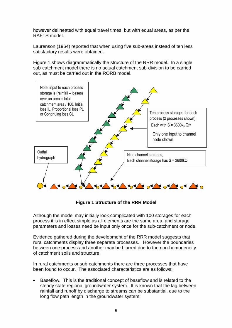
however delineated with equal travel times, but with equal areas, as per the RAFTS model. Laurenson (1964) reported that when using five sub-areas instead of ten less satisfactory results were obtained. Figure 1 shows diagrammatically the structure of the RRR model. In a single sub-catchment model there is no actual catchment sub-division to be carried out, as must be carried out in the RORB model.

Ten process storages for each process (2 processes shown) Each with S = 3600kp Qm

Nine channel storages, Each channel storage has S = 3600kQ

Outfall hydrograph

Note: input to each process storage is (rainfall � losses) over an area = total catchment area / 100, Initial

loss IL, Proportional loss PL

or Continuing loss CL

Only one input to channel

node shown

Figure 1 Structure of the RRR Model

Although the model may initially look complicated with 100 storages for each process it is in effect simple as all elements are the same area, and storage parameters and losses need be input only once for the sub-catchment or node. Evidence gathered during the development of the RRR model suggests that rural catchments display three separate processes. However the boundaries between one process and another may be blurred due to the non-homogeneity of catchment soils and structure. In rural catchments or sub-catchments there are three processes that have been found to occur. The associated characteristics are as follows: Baseflow. This is the traditional concept of baseflow and is related to the

steady state regional groundwater system. It is known that the lag between rainfall and runoff by discharge to streams can be substantial, due to the long flow path length in the groundwater system;

6

Slow flow, most probably capillary fringe flow. This mechanism acts with a lag from rainfall to stream flow that is less than that of the baseflow above, due to the quicker response time from rainfall to runoff into the stream; and

Fast flow, most probably similar to Hortonian overland flow, either from a part of the catchment area, or the full catchment area. The response time of this mechanism is short compared with the two above, as no groundwater flow is involved.

The RRR model structure can be used on each sub-catchment of a total catchment model. This allows the variation across the catchment of rainfall or model loss or storage parameters. To allow the use of the RRR model is this way generalised parameters are needed, to account for changes in storage lag as a result of the catchment area of each sub-catchment. As the channel lag is linear it could be expected that for rural catchments the channel lag will be highly correlated with the mainstream length of the catchment. For the purposes of the derivation of a generalised parameter, a variable representing the characteristic flood wave velocity vc is introduced. This can be related to channel lag k on the assumption of the ten channel reaches. Equation 1 relates vc to k, allowing for the number of channel reaches and the conversion of lag time, which is in hours.

k

dv

c36

Equation 1

Where vc is the channel characteristic flood wave velocity (m/sec) d is the longest flow path length (km) k is the channel storage lag parameter (hrs) However the non-linearity of most process storages creates a problem in that the storage lag depends on the storage outflow, which is in turn dependent on the modelled catchment area. For this reason a new variable is used, being the catchment characteristic lag parameter, cp, where:

k c Ap pm 1

Equation 2

Where A is the catchment or sub-catchment area (km2) m is the exponent in the process storage relationship kp is the process storage parameter The reason for the use of this parameter is as follows. The lag of a single process storage is given by the equation:

lag k Qpm1

Equation 3

7

Where Q is the total flow into the channel storages. But it can be seen that the lag of the catchment process storages changes as the area of the modelled catchment changes, as Q is dependent on the area represented by the process storages. If cp is used the lag is then:

lag c A Q

cQA

pm m

p

m

1 1

1

Equation 4

It can be seen that lag will not now depend on catchment area as Q/A is constant. This constant Q/A follows from the structure of the RRR model, which assumes a constant catchment width, meaning that flow into the channel (Q) is proportional to the channel length and thus the area represented by the series of process storages (A). Since the lag is for a single sub-catchment the effect of rainfall distribution or catchment topography need not be considered. There will be a characteristic lag parameter associated with the first two runoff processes, which will be labelled cp1 and cp2. The third runoff process (fast flow) has been found to have effectively zero lag. Urban catchments or sub-catchments display two runoff processes contributing to a pipe system, being the contribution from the directly connected impervious area (the connected area), and the balance, termed the unconnected area. The unconnected area is the sum of the supplementary paved and pervious areas as used in other models such as DRAINS. The process lag of the directly connected and unconnected areas has been found by calibration of the RRR model on the Glenelg and Paddocks catchments. The channel lag for urban catchments or sub-catchments is dependent on the mean gutter and pipe flow times. A relationship was derived by Kemp (2002), as flows:

hoursxs

Lx

sr

Lxk

g

gn

i ii

pi 33

1667.0

3 101063.310333.0

Equation 5

Where Lpi Is the length of the ith pipe reach of the longest pipe length

within the catchment ri Is the hydraulic radius of that pipe (m) si Is the slope of that pipe (m/m) Lg Is the mean gutter flow length sg Is the mean gutter slope (m/m)

8

3 DEVELOPING THE RRR MODEL The structure of the RRR model was similar to that used on Brown Hill and Keswick Creeks (Transport SA, 2004). A separate model was set up for each creek. Although there may be some interaction between the creeks for larger flows, the hydrology model was to provide inflow hydrographs only, so the added complexity was not required. In each model sub-catchment boundaries were placed firstly at locations where hydrographs were required to be provided in accordance with the brief. Further examination and discussion led to the inclusion of further sub-division to provide adequate inflow information to the hydraulic model. The hydraulic model could receive either concentrated inflows, or inflow distributed along a channel reach. The percentages of directly connected impervious area in the urban parts of the models was based on previous work carried out in the Glenelg and Paddocks catchments (Kemp & Lipp, 1999) and the calibrated model for the Brown Hill and Keswick Creeks. Typical percentages ranged from 27% for urban development to 95% in the city centre. The characteristic velocity for channels in the urban area ranged from 1.5m/sec for unlined channels to 3m/sec for concrete lined channels. The channel storage delay time in urban areas is a function of gutter and pipe lengths and slopes within each sub-catchment.

4 FITTING THE RRR MODELS

4.1 Available Data The catchments of First to Fifth Creeks are now reasonably well instrumented, although most of the pluviometers and stream gauges have only been installed in the past few years. An exception to this is First Creek above the waterfall in Waterfall Gully, which has record dating back to 1976. It is thus the only station within the study area for which a flood frequency analysis can be carried out with any degree of confidence. Table 1 and Table 2 list the stations within the study area.

9

Table 1 First to Fifth Creeks - Stream Gauging Stations

Station Number Latitude Longitude Start Date First Creek � Waterfall Gully

AW504517 -34.972 138.680 1976

First Creek � below Chambers Gully

BM523746 -34.950 138.670

First Creek � Botanic Gardens

AW504578 -34.917 138.605 1996

Second Creek � Stepney BM023104 -34.911 138.627 June 2003 Third Creek � Forsyth Court

AW504579 -34.892 138.642 1996

Fourth Creek � Stradbroke BM023086 -34.893 138.685 January 2003

Fifth Creek � Athelstone BM023094 -34.874 138.690

Table 2 First to Fifth Creeks - Pluviometer Stations

Station Number Latitude Longitude Start Date Cleland BM523860 -34.9575 138.6889 March 2001 Burnside BM023042 -34.9388 138.6605 September 2001 Seaview BM023085 -34.8946 138.8100 November 2001 Black Hill BM023896 -34.8758 138.7103 January 2003 Stradbroke BM023086 -34.8931 138.6853 January 2003 Payneham Pool BM023101 -34.8925 138.6422 March 2003 Stepney BM023104 -34.9111 138.6272 June 2003 Ashton BM023867 -34.9342 138.7465 July 1992 Kent Town BM023090 -34.9231 138.6206 1977 Mount Lofty AW504552 -34.9832 138.7059 September 1984 Beaumont BM023114 -34.956 138.658 1994 Eagle on the Hill BM023874 -34.976 138.671 August 2000 Glenside AW504906 -34.95 138.63 February 1995 Montacute BM023892 -34.833 138.757 August 2001

4.2 First Creek � Waterfall Gully (AW504517) The First Creek catchment to the Waterfall Gully gauging station is situated in the hills face zone of the Mount Lofty Ranges, to the east of Adelaide. It is a steep catchment, and is substantially in natural condition, with most of the catchment being contained within the Cleland Conservation Park. It has a catchment area of 4.89km2. The underlying rock is mainly quartzite. Rainfall data from the Mount Lofty gauge (AW504552) at the upper end of the catchment was used as it was the only available pluviometer data for the events modelled. Baseflow was present in all modelled events, but there was no evidence of fast runoff.

10

Table 3 First Creek at Waterfall Gully - RRR Calibrated Parameters

Event Start Date PL1 IL2 (mm) PL2 k kp1 kp2 30/06/1986 0.75 91.6 0.88 0.390 2.466 0.480 01/08/1986 0.65 30.6 0.74 0.891 3.594 0.656 21/06/1987 0.73 28.6 0.89 0.136 5.954 0.587 14/07/1987 0.53 19.47 0.93 0.026 4.524 0.815 14/08/1990 0.76 21.79 0.83 0.081 2.892 0.411 29/08/1992 0.62 13.57 0.90 0.038 8.040 0.769 14/09/1992 0.60 61.15 0.76 0.010 3.855 0.490 Mean 0.66 39.25 0.84 0.347 3.365 0.660

4.3 First Creek Downstream Botanic Gardens (AW504578) The First Creek gauging station downstream of the Botanic Gardens was opened in 1996. The largest seven peak flow events were chosen to verify the RRR model developed using normal RRR model parameter values for urban areas. In all cases it was found that there was very little contribution from the rural portion of the catchment. Ponding within the east parklands was included within the model to match the shape of the recorded hydrographs. In particular the gross pollutant trap installed on Botanic Creek in May � June 1999 was included, with details based on site observations and drawings supplied by the Torrens Catchment Water Management Board. The City of Adelaide supplied survey of the parks, from which storage � level relationships were derived. Minor changes were made to the directly connected impervious area within the urban area, but with only a single gauging station no information could be gained as to whether individual parts of the model were correct. The same model was used for all events, so that the process could be considered to be a verification of the model. Pluviometer data from Beaumont (BM023114), Cleland (BM523860), Mount Lofty (AW504552), Eagle on the Hill (BM023874), Glenside (AW504906) and Kent Town (BM023090) was used. From examination of the shape of the recorded hydrographs it was determined that there was no significant rural contribution for any of the events examined. Table 4 and Figure 2 summarise the fit produced by the final RRR model for historical storm events.

11

Table 4 First Creek Downstream Botanic Gardens - Calibrated RRR Model Fit

Storm Date

Gauged Peak Q (m3/sec)

Predicted Peak Q (m3/sec)

Gauged Vol (m^3)

Predicted Vol (m^3)

6 February 1997 9.45 10.66 56960 733905 October 1998 10.87 12.03 140400 106900

22 May 1999 13.92 22.05 98370 11770015 May 2000 11.53 9.88 69440 579405 June 2001 13.02 16.42 166350 1774006 June 2003 9.94 7.20 53760 44170

30 October 2003 3.31 4.46 49860 49560

First Creek Predicted Peak Flow

0.00

5.00

10.00

15.00

20.00

25.00

0.00 5.00 10.00 15.00 20.00 25.00

Gauged Flow (m^3/sec)

Pre

dic

ted

Pea

k (m

^3/s

ec)

First Creek Predicted Volumes

0

20000

40000

60000

80000

100000

120000

140000

160000

180000

200000

0 50000 100000 150000 200000

Gauged Volume (m^3)

Pre

dic

ted

Vo

lum

e (m

^3)

Figure 2 First Creek Downstream Botanic Gardens - Claibrated RRR Model Fit

Plots of the recorded and predicted hydrographs for all events are given in Appendix 2.

4.4 Second Creek at Stepney (BM023104) The Second Creek gauging station at Stepney was opened in June 2003. Five storm events after this date were used for the verification of the RRR model for this catchment. The detention basin in Kensington Gardens was included in the model, based on information received from the City of Burnside. Pluviometer data from Cleland (BM523860), Burnside (BM023042), Seaview (BM023085), Kent Town (BM023090) and Stepney (BM023104) was used. Only minor changes were made in the model to fit the recorded hydrographs. All of the events showed some contribution from the rural catchment, although in terms of the total flow at the gauging station the contribution was minor. This made the model relatively insensitive to the rural loss values used. Consequently calibrating for rural losses was difficult but greater confidence in this regard can be given to those storms having a larger rural flow contribution.

12

Table 5 Second Creek at Stepney - Calibrated Rural Losses

Event Date Process IL (mm)

PL Total Rainfall (mm)

Effective Rainfall (mm)

1 (base flow) 0 0.82 44.4 4.44 26 June 2003 2 (slow flow) 0 0.90 0.17 1 (base flow) 0 0.82 13.8 2.84 24 July 2003 2 (slow flow) - - 0.00 1 (base flow) 0 0.82 12.4 1.24 4 August 2003 2 (slow flow) 0 0.9 0.04 1 (base flow) 0 0.65 33.2 11.62 23 August

2003 2 (slow flow) 15 0.90 1.82 1 (base flow) 0 0.82 20.6 3.71 30 October

2003 2 (slow flow) 0 0.90 2.06 Table 6 and Figure 3 summarise the model calibration.

Table 6 Second Creek at Stepney - RRR Model Fit

Storm Date



Gauged Vol (m^3)

Predicted Vol (m^3)

26 June 2003 15.21 13.42 240300 21870024 July 2003 9.08 5.87 49830 45670

4 August 2003 10.28 8.46 57260 5703023 August 2003 7.49 7.37 178500 168700

30 October 2003 7.63 7.66 70130 92530

Second Creek Predicted Peak Flow

0.00

2.00

4.00

6.00

8.00

10.00

12.00

14.00

16.00

0.00 5.00 10.00 15.00 20.00

Gauged Peak (m^3/sec)

Pre

dic

ted

Pea

k (m

^3/s

ec)

Second Creek Predicted Volumes

0

50000

100000

150000

200000

250000

300000

0 50000 100000 150000 200000 250000 300000

Gauged Volume (m^3)

Pre

dic

ted

Vo

lum

e (m

^3)

Figure 3 Second Creek Stepney - Calibrated RRR Model Fit

The results of the verification show good fits to both the peak flows and runoff volumes. Hydrograph plots are given in Appendix 2.

13

4.5 Third Creek at Forsyth Grove, Felixstow The Third Creek gauging station has been in operation since 1996, but there has been insufficient rainfall information on which to base model calibration until the installation of pluviometers at Seaview (AW023085) in November 2001 and Payneham Pool (AW023101) in March 2003. Nine large events between 2002 and 2004 were chosen for modelling, with the Kent town pluviometer being used where the Payneham pool pluviometer was not available.

Table 7 Third Creek at Forsyth Grove - Calibrated RRR Model Fit

Storm Date



Gauged Vol (m^3)

Predicted Vol (m^3)

27 June 2002 4.49 6.72 42000 70340 18 May 2002 4.70 2.70 16290 15170

25 November 2002 5.80 9.23 20330 39680 31 October 2003 3.18 5.94 36810 41860

1 November 2003 4.57 1.98 4569 4730 19 December 2003 1.15 1.66 7199 8787 21 December 2003 1.44 4.45 10560 17770

17 May 2004 1.31 2.99 10400 47310 28 May 2004 0.76 2.74 3517 6511

Third Creek Predicted Peak Flow

0.00

1.00

2.00

3.00

4.00

5.00

6.00

7.00

8.00

9.00

10.00

0.00 2.00 4.00 6.00 8.00 10.00

Gauged Peak Flow (m^3/sec)

Pre

dic

ted

Pea

k F

low

(m

^3/s

ec)

Third Creek Predicted Volumes

0

10000

20000

30000

40000

50000

60000

70000

80000

0 20000 40000 60000 80000

Gauged Volume (m^3)

Pre

dic

ted

Vo

lum

e (m

^3)

Figure 4 Third Creek at Forsyth Grove - Calibrated RRR Model Fit

The hydrographs for the events are contained in Appendix 2. The fit for Third Creek was not as good as for First and Second Creek, due mainly to the poorer pluviometer data being available. There was no rural runoff apparent for any of the events modelled.

4.6 Fifth Creek at Athelstone The gauging station is located on a natural open channel, without a weir or other control. For this reason the accuracy of the gauged flows is not as good as at other stations that have been used for calibration.

14

Four storm events were used for calibration of the model, all of which occurred in 2003. The peak flows ranged from 1.5 m3/sec to 2 m3/sec. The depth of flow in the channel at 2 m3/sec is 0.5m. No significant rural contribution was evident in any of the events modelled. Pluviometer data from Black Hill (BM023896) and Montacute (BM023892) was used.

Table 8 Fifth Creek at Athelstone -� Calibrated RRR Model Fit

Storm Date



Gauged Vol (m^3)

Predicted Vol (m^3)

30 April 2003 2.04 2.13 18530 636823 May 2003 1.55 2.24 13290 1859026 June 2003 1.77 1.85 47120 17580

21 December 2003 1.29 0.75 12910 2071

Fifth Creek Predicted Peak Flows

0.00

0.50

1.00

1.50

2.00

2.50

0.00 0.50 1.00 1.50 2.00 2.50

Gauged Peak (m^3/sec)

Pre

dic

ted

Pea

k (m

^3/s

ec)

Fifth Creek Predicted Volumes

0

5000

10000

15000

20000

25000

30000

35000

40000

45000

50000

0 10000 20000 30000 40000 50000

Ga uge d Vol ume ( m^3 )

Figure 5 Fifth Creek at Athelstone - RRR Model Fit

The predicted peak flows were satisfactory, given the standard of the rating at the gauging station. However the runoff volume is under estimated. This also may be due to the rating, with significant volumes passing the gauging station at low flow depths, where the rating would be most in error.

4.7 Sixth Creek The Sixth Creek catchment has also been calibrated, as it is an adjoining catchment to the catchments being examined. The calibration was carried out as part of the work undertaken by Kemp (2002). The Sixth Creek catchment is a steep catchment in the high rainfall area of the Mount Lofty Ranges. There is a substantial amount of natural vegetation. It has a catchment area of 43.8km2.

15

Table 9 Sixth Creek Calibration Results

Event Start Date

PL1 IL2 (mm) PL2 k kp1 kp2

21/06/1987 0.88 41.48 0.68 0.207 13.45 0.848 15/09/1991 0.54 37.70 0.60 0.357 2.175 0.768 29/08/1992 0.59 37.60 0.63 0.256 2.886 0.502 07/10/1990 0.52 16.27 0.57 0.263 8.077 1.308 17/12/1992 0.75 11.13 0.88 0.302 2.598 0.461 28/09/1996 0.62 29.61 0.60 0.497 3.396 0.680

Mean 0.63 28.92 0.65 0.329 4.829 0.763

5 FLOOD FREQUENCY ANALYSIS Flood Frequency analysis was carried out on the First Creek catchment to the waterfall and adjacent catchments to determine parameters for the RRR model that will match historical flows. Annual maximum flows were determined for the First Creek catchment (AW504517), the Brown Hill Creek catchment (AW504901) and Sixth Creek (AW504523).

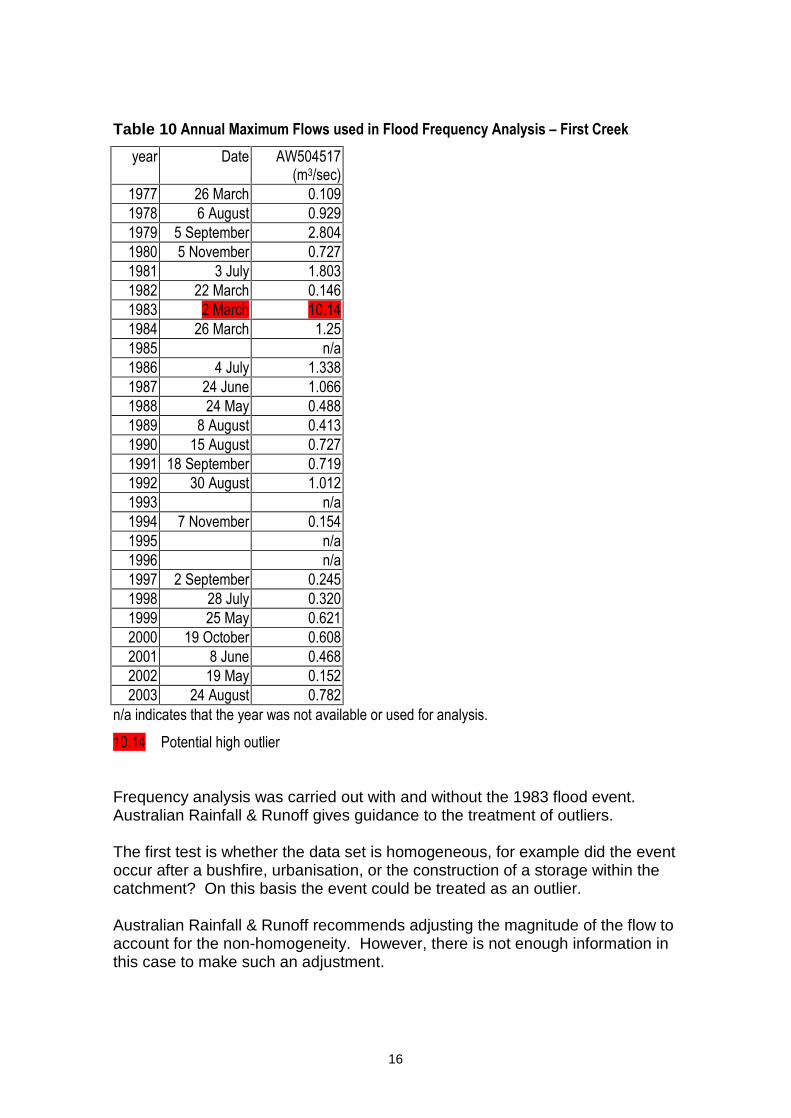
5.1 First Creek Log normal frequency distribution was used, as was used in the study of the upper Onkaparinga River (Transport SA, 2003). This distribution fitted the recorded values in most cases, and was confirmed by continuous simulation of long term flows at Hougraves Weir on the Onkaparinga River to be a reasonable distribution. No low flows were censored, however the high flow that occurred in March 1983 needs special consideration. This high flow is more than double any other flow in the period of record, and occurred shortly after a bushfire burnt out the catchment. It could thus assumed to be an outlier and rejected as the catchment was not in the same condition as all the other years.

16

Table 10 Annual Maximum Flows used in Flood Frequency Analysis � First Creek

year Date AW504517

(m3/sec)

1977 26 March 0.109

1978 6 August 0.929

1979 5 September 2.804

1980 5 November 0.727

1981 3 July 1.803

1982 22 March 0.146

1983 2 March 10.14

1984 26 March 1.25

1985 n/a

1986 4 July 1.338

1987 24 June 1.066

1988 24 May 0.488

1989 8 August 0.413

1990 15 August 0.727

1991 18 September 0.719

1992 30 August 1.012

1993 n/a

1994 7 November 0.154

1995 n/a

1996 n/a


1998 28 July 0.320

1999 25 May 0.621

2000 19 October 0.608

2001 8 June 0.468

2002 19 May 0.152

2003 24 August 0.782

n/a indicates that the year was not available or used for analysis.

10.14 Potential high outlier

Frequency analysis was carried out with and without the 1983 flood event. Australian Rainfall & Runoff gives guidance to the treatment of outliers. The first test is whether the data set is homogeneous, for example did the event occur after a bushfire, urbanisation, or the construction of a storage within the catchment? On this basis the event could be treated as an outlier. Australian Rainfall & Runoff recommends adjusting the magnitude of the flow to account for the non-homogeneity. However, there is not enough information in this case to make such an adjustment.

17

The second test is a statistical test, based on the Grubbs and Beck (1972) test, where a high outlier threshold is identified. The equation used to indicate high outliers is:

SKMX NH Where XH = High outlier threshold in log units M = Mean of the logs of the annual floods excluding zero and

very low events S = Standard deviation of logs of flows KN = Value from table 2.8 of book 4 of Australian Rainfall &

Runoff for sample size N annual floods = An adjustment factor, depending of N and g, the skew of the

logs of floods In this case N = 23, M = -0.194, S = 0.444 and from table 2.6 of Australian Rainfall & Runoff, KN = 2.624 and from table 2.7, = 1.01. The log of the high outlier threshold XH is then 0.983, or the threshold is 9.6m3/sec. On this basis the flow can be treated as an outlier.

Log normal probability plot: 2-parameter Log Normal

ARI (yrs)

-1.000

-0.460

0.080

0.620

1.160

1.700

Log10 Flow

1.5 2 5 10 20 50100200500

Gauged flow

Exp parameter quantile

Expected prob quantile

90% limits

Figure 6 First Creek Flood Frequency - 1983 Flood Included

18


ARI (yrs)

-1.000

-0.520

-0.040

0.440

0.920

1.400

Log10 Flow

1.5 2 5 10 20 50100200500

Gauged flow



90% limits

Figure 7 First Creek Flood Frequency - 1983 Flood Excluded

The frequency distribution is given in Table 11. Also given in the table are the flows if the 1983 flood is not treated as an outlier. In addition a report was found in the Advertiser newspaper dated 6 September 1979, where a resident of Waterfall Gully stated that the flood on the previous day was the largest for the 10 years of their residency. If a further 8 years of flows (1969 � 1976) less than the recorded peak of 2.8m3/sec are added to the data series the amended frequency can be calculated. Table 11 gives a summary of the distributions fitted. Table 12 gives the confidence limits for the distribution with the 1983 flood treated as an outlier, and with 8 extra years less than 2.8m3/sec.

19

Table 11 First Creek at Waterfall Flood Frequency Distribution

Station Area

(km2)

1:10 AEP

(m3/sec)

1:20 AEP

(m3/sec)

1:50 AEP

(m3/sec)

1:100 AEP

(m3/sec)

AW504517 � 1983 as an outlier 4.9 1.71 2.34 3.34 4.23

AW504517 � all years of record 4.9 2.44 3.57 5.48 7.28

AW504517 � 1983 as an

outlier, 8 extra years less than

2.8m3/sec added

4.9 1.62 2.21 3.11 3.92

AW540517 � all years of record

plus 8 extra years less than

2.8m3/sec added

4.9 2.22 3.20 4.83 6.37

Table 12 First Creek at Waterfall Flood Frequency Confidence Limits

Annual Exceedance Probability

Predicted Flow (m3/sec)

10% confidence limit (m3/sec)


1:20 2.22 1.51 3.65 1:50 3.13 2.02 5.62 1:100 3.95 2.45 7.51

5.2 Sixth Creek The Sixth Creek catchment has an area of 43.8km2, and lies immediately adjacent to and east of the Second, Third, Fourth and Fifth Creek catchments.

20

Table 13 Annual Maximum Flows Used in Flood Frequency Analysis - Sixth Creek

year AW504523

(m3/sec)

1978 5 July 25.07


1980 5 November 13.10

1981 26 June 81.0

1982 n/a

1983 8 August 15.70

1984 18 August 10.07

1985 6 August 11.43

1986 6 December 17.03

1987 24 June 28.3

1988 24 May 12.14

1989 n/a

1990 n/a

1991 18 September 27.12

1992 30 August 81.7

1993 7 July 5.14

1994 23 June 2.61

1995 22 July 28.36

1996 4 August 17.73


1998 28 July 9.98

1999 9 August 8.19



2002 20 May 2.68

2003 25 July 10.12

n/a indicates that the year was not available or used for analysis.

The distribution was assumed to be log normal, in common with other frequency distributions examined in the Mount Lofty Ranges.

Table 14 Sixth Creek Flood Frequency Confidence Limits

AEP Predicted Flow (m3/sec)



1:20 63.1 41.1 111 1:50 91.5 55.8 177 1:100 117 68.4 242

21


ARI (yrs)

0.230

0.744

1.258

1.772

2.286

2.800

Log10 Flow

1.5 2 5 10 20 50100200500

Gauged flow



90% limits

Figure 8 Sixth Creek Flood Frequency Distribution

5.3 Brown Hill Creek The Brown Hill Creek catchment to Scotch College has a catchment area of 17.6km2, and is adjacent to the First Creek catchment. Flood frequency analysis has been carried out on the 14 full years of flow data available at Scotch College, with the addition of one historical event in 1981 that was described in the WBCM report (WBCM, 1984). An allowance was made in the plotting position for the eight years of flow where no record is available.

22

Table 15 Annual Maximum Flows Used in Flood Frequency Analysis - Brown Hill Creek

year Date AW504901

(m3/sec)

1990 15 August 1.97


1992 30 August 5.01

1993 7 July 3.67

1994 2 October 0.69

1995 22 July 3.40

1996 22 August 4.09


1998 28 July 1.42

1999 25 May 2.27



2002 20 May 1.45

2003 24 August 2.89


ARI (yrs)

-0.340

0.108

0.556

1.004

1.452

1.900

Log10 Flow

1.5 2 5 10 20 50100200500

Gauged flow

Censored flow



90% limits

Figure 9 Brown Hill Creek Flood Frequency Distribution

23

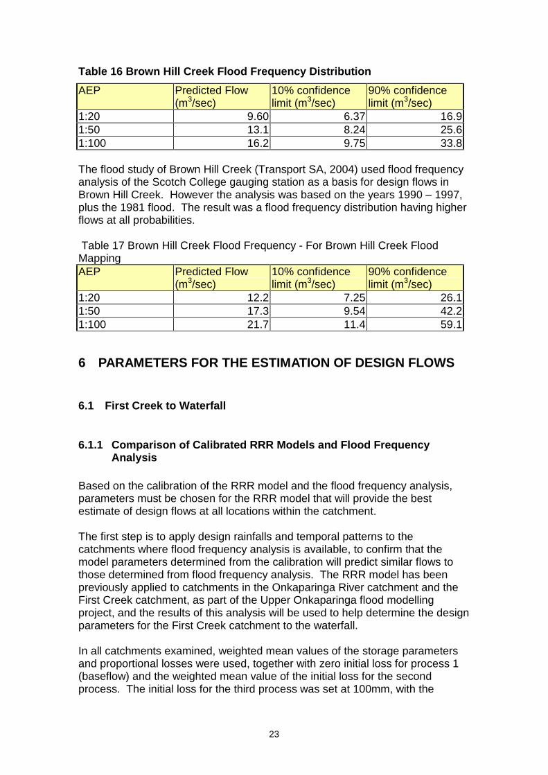
Table 16 Brown Hill Creek Flood Frequency Distribution

AEP Predicted Flow (m3/sec)



1:20 9.60 6.37 16.9 1:50 13.1 8.24 25.6 1:100 16.2 9.75 33.8 The flood study of Brown Hill Creek (Transport SA, 2004) used flood frequency analysis of the Scotch College gauging station as a basis for design flows in Brown Hill Creek. However the analysis was based on the years 1990 � 1997, plus the 1981 flood. The result was a flood frequency distribution having higher flows at all probabilities. Table 17 Brown Hill Creek Flood Frequency - For Brown Hill Creek Flood Mapping AEP Predicted Flow

(m3/sec) 10% confidence limit (m3/sec)


1:20 12.2 7.25 26.1 1:50 17.3 9.54 42.2 1:100 21.7 11.4 59.1

6 PARAMETERS FOR THE ESTIMATION OF DESIGN FLOWS

6.1 First Creek to Waterfall

6.1.1 Comparison of Calibrated RRR Models and Flood Frequency Analysis

Based on the calibration of the RRR model and the flood frequency analysis, parameters must be chosen for the RRR model that will provide the best estimate of design flows at all locations within the catchment. The first step is to apply design rainfalls and temporal patterns to the catchments where flood frequency analysis is available, to confirm that the model parameters determined from the calibration will predict similar flows to those determined from flood frequency analysis. The RRR model has been previously applied to catchments in the Onkaparinga River catchment and the First Creek catchment, as part of the Upper Onkaparinga flood modelling project, and the results of this analysis will be used to help determine the design parameters for the First Creek catchment to the waterfall. In all catchments examined, weighted mean values of the storage parameters and proportional losses were used, together with zero initial loss for process 1 (baseflow) and the weighted mean value of the initial loss for the second process. The initial loss for the third process was set at 100mm, with the

24

proportional loss consistent with the proportional losses for the other two processes. One problem with the estimation of design flows is that the initial and proportional loss for process 3 (fast flow) is not usually determined from calibration, as the process occurs rarely. In most cases PL3 must be estimated. From other calibrations undertaken that show runoff from process 3, it has been found that the proportional loss is generally of the same order as that of process 1 and 2. Table 18 gives a summary of the proportional losses found in calibrated catchments. Care must be taken in the application of the RRR model as losses for all processes are related to the total rain falling on the catchment. Thus, with a low proportional loss applied to each process it is possible that the outflow volume from the catchment could exceed the rainfall input volume. For example if the initial and proportional losses for each of the three processes were zero, the volume outflow would be three times the rainfall volume. The value of PL3 to be used for design purposes must be reviewed in the derivation of design losses, to avoid the situation where runoff is exceeding rainfall for part of the storm.

Table 18 Proportional Losses Assumed for the Onkaparinga River Catchments, and First Creek

Catchment Station Number

PL1 PL2 PL3

Cox AW503526 0.82 0.76 0.80 (estimated) Aldgate AW503509 0.75 0.60 0.65 (from 1 calibration) Inverbrackie AW503508 0.74 0.42 0.70 (estimated) Lenswood AW503507 0.68 0.58 0.60 (estimated) Scott AW503502 0.78 0.76 0.75 (estimated) Echunga AW503506 0.89 0.72 0.82 (from 1 calibration) Houlgraves AW503504 0.78 0.61 0.56 First AW504517 0.66 0.84 0.75 (estimated) The initial loss of process 3 is also unknown, but 100mm is assumed for initial comparison. Table 19 gives the comparison of flood frequency analysis and design flows with the losses from Table 18, and confirms that there is no significant bias. However there are some differences, particularly significant being the Echunga Creek and the Houlgraves catchment.

25

Table 19 Comparison of Flood Frequency and Calibrated RRR Model

Catchment 1:10 AEP RRR model (m3/sec)

1:10 AEP flood frequency (m3/sec)

1:100 AEP RRR model (m3/sec)

1:100 AEP flood frequency (m3/sec)

Cox 5.7 6.7 9.3 9.4 Aldgate 14.4 13.2 24.4 22.6 Inverbrackie 13.2 12.3 22.9 27.0 Lenswood 24.2 25.9 61.3 65.9 Scott 18.5 15.6 31.3 31.7 Echunga 26.0 30.6 42.6 66.9 Houlgraves 212 294 509 657 First 1.70 1.71 5.7 4.2

6.1.2 Derivation of Rural Design Losses From the calibrated RRR models design losses must be determined. This is necessary because design storms represent bursts within longer duration storm events. The initial losses derived by calibration may not be appropriate when applied with design rainfalls. In recent times work has been carried out by the CRC for Catchment Hydrology on the derivation of design losses for flood estimation (Hill et al, 1998). Another problem is that the calibrated mean losses may not be truly representative of mean catchment conditions, to be used with design rainfalls. Examination of the calibrated proportional losses show wide variation. As the calibrated mean losses is only based on a limited number of events it is considered legitimate, based on other information, to vary the mean losses determined in the calibration to obtain design losses. As the station flood frequency flow is based on recorded data it is considered that emphasis should be given to the station flood frequency flows. It was therefore decided to use these flows as the best estimate available and adjust the RRR mean losses to match the flood frequency analysis flows, where this was possible while keeping to within reasonable loss figures. Therefore for the First Creek catchment the PL3 and IL3 were adjusted to give reasonable agreement with the 1:100 Annual Exceedance Probability (AEP) flow (the predicted flow being 4.6m3/sec). The IL3 was kept at 100mm and PL3 adjusted.

26

Table 20 Calibrated and Design RRR Model Design Loss Parameters � First Creek Catchment

IL2 (mm) IL3 (mm) PL1 PL2 PL3 Calibrated / Estimated

39.52 n/a 0.66 0.84 0.75

Design 39.52 100 0.66 0.84 0.85

6.2 Other Rural Catchments All other rural catchments within the study area do not have gauging stations with sufficient data for calibration of the RRR model, apart from Second Creek where some values were obtained by calibration. However the rural catchment is a small proportion of the gauged Second Creek catchment, and only a small number of events were used for calibration. Parameter values must therefore be determined by other means. Determining a regional relationship for the parameter values generally does this. An example is the RORB storage parameter kc is determined as kc = 0.6A0.67, where A is the catchment area. The area alone determines the catchment lag. The RRR model was developed to better understand catchment lag. It automatically takes into account the affect of area on catchment lag, and thus is more likely to demonstrate what other factors have an effect. Kemp (2003) and Kemp (2002) examined the factors that affect both storage and loss parameters with the conclusion that:

Analysis has shown that the soil depth and the root zone water holding capacity of the soil are the main determinants of process storage parameters. The presence of native vegetation on the catchment also has an effect, increasing the process storage lag over that expected for other land uses. The process lags for base and slow flow are related, which is not surprising since they are both governed by the two main determining factors, being root zone water holding capacity and soil depth. The response of a catchment will vary depending on what part of the catchment is contributing the runoff, and what runoff processes are occurring. The catchment will not have one identifiable response time, rather the response will change with each event, and the accompanying difference in contributing soil type and depth.

Although the factors that affect lag have been examined, good relationships between the parameter values and catchment physical parameters could not be determined.

27

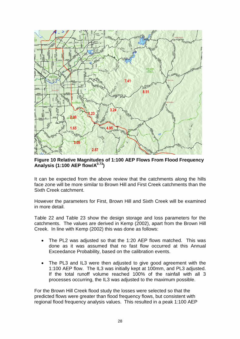
It is proposed therefore that catchment parameters for the ungauged catchments will be determined using parameter values from similar catchments that have been calibrated to actual storm events. To determine similarity the factors that affect catchment losses and catchment lag will be used. The catchments along the hills face have similar slopes, but the geology and associated soils vary. The runoff characteristics of gauged catchments near to the First to Fifth Creek catchments were examined to determine which catchments could be considered to be similar, and thus be expected to have similar parameter values. Flood frequency analysis was carried out with all available years of record. The relative magnitude of the 1:100 AEP flows were then determined by adjusting the flood frequency flow by a factor to account for the effect of catchment area. The factor A0.73 was used, based on Eusuff (1995).

Table 21 Mount Lofty Ranges Catchments - Relative 1:100 AEP Flows

Catchment Station Area (km) 1:20 AEP (m3/sec)

1:100 AEP (m3/sec)

1:100AEP/A^0.73

First Creek AW504517 4.9 2.21 3.92 1.23 Minno AW504519 18 10.8 13.6 1.65 Brown Hill Creek - Scotch AW504901 17.6 9.6 16.2 2.00 Scott AW504502 26.8 20 31.7 2.87 Sturt u/s Minno AW504518 19 15.7 26.4 3.08 Cox AW503526 4.3 7.5 9.4 3.24 Aldgate AW503509 8 15.9 22.6 4.95 Sixth AW504523 43.8 63.1 117 7.41 Lenswood AW503507 16.5 35.8 65.9 8.51 It can be seen in Table 21 and Figure 10 that the catchments to the west and south have lower flows than the catchments north and east of Mount Lofty. In particular the First Creek and Brown Hill creek catchments, in the hill face zone have much lower relative flows than the adjacent catchments to the east of Mount Lofty (Aldgate, Cox and Sixth Creeks).

28

1.23

1.65

2.00

2.87

3.08

3.24

4.95

7.41

8.51

Figure 10 Relative Magnitudes of 1:100 AEP Flows From Flood Frequency Analysis (1:100 AEP flow/A0.73)

It can be expected from the above review that the catchments along the hills face zone will be more similar to Brown Hill and First Creek catchments than the Sixth Creek catchment. However the parameters for First, Brown Hill and Sixth Creek will be examined in more detail. Table 22 and Table 23 show the design storage and loss parameters for the catchments. The values are derived in Kemp (2002), apart from the Brown Hill Creek. In line with Kemp (2002) this was done as follows:

The PL2 was adjusted so that the 1:20 AEP flows matched. This was done as it was assumed that no fast flow occurred at this Annual Exceedance Probability, based on the calibration events.

The PL3 and IL3 were then adjusted to give good agreement with the

1:100 AEP flow. The IL3 was initially kept at 100mm, and PL3 adjusted. If the total runoff volume reached 100% of the rainfall with all 3 processes occurring, the IL3 was adjusted to the maximum possible.

For the Brown Hill Creek flood study the losses were selected so that the predicted flows were greater than flood frequency flows, but consistent with regional flood frequency analysis values. This resulted in a peak 1:100 AEP

29

flow prediction at Scotch College of 26.0m3/sec, compared with the at station flood frequency flow of 21.7m3/sec. The Sixth Creek flood frequency was difficult to reproduce with design losses, with all rainfall being converted to runoff with three processes occurring. The predicted design peak flow with an initial loss for process 3 of 75mm was 62.7m3/sec for 1:20 AEP (flood frequency 63.1m3/sec) and 101m3/sec for 1:100 AEP (flood frequency 117m3/sec). The flood frequency flow is possibly high due to two storm events having occurred on the Sixth Creek catchment in the period of record that can be considered rare events (June 1981 and August 1992, both nearly 1:50 AEP flows according to the flood frequency analysis.

Table 22 Hills Face and Adjacent Catchments - Design Storage Parameters

Catchment Vc (m/sec) cp1 cp2 First Creek 0.47 3.08 0.42 Brown Hill Creek 1.24 1.72 0.46 Sixth Creek 1.42 2.267 0.358

Table 23 Hills Face and Adjacent Catchments - Design Losses

Catchment IL1 (mm) PL1 IL2 (mm) PL2 IL3 (mm) PL3 Brown Hill Creek - Calibrated

0 0.82 17.5 0.77 n/a n/a

Brown Hill Creek design (based on new flood frequency)

0 0.82 17.5 0.86 100 0.85

Brown Hill Creek design (Flood Study values)

10 0.82 35 0.76 50 0.78

Sixth Creek - Calibrated

0 0.63 28.9 0.65 n/a n/a

Sixth Creek - Design

0 0.63 28.9 0.65 75 0.72

n/a � no events showed process 3 runoff in calibration The Brown Hill Creek catchment is dominated by the Saddleworth formation, which includes dolomites and slates. The First Creek catchment above the waterfall is almost all Stonyfell Quartzite. Examination of the geological mapping indicates that for the First to Fifth Creek catchments the geology is a combination of these two types. The creek catchments are also similar in respect to average slopes and vegetation cover. It is proposed therefore that either design values from the First Creek catchment (AW504517) or the Brown Hill Creek catchment (AW504901) be used. The

30

rural part of each creek catchment was sub-divided into sub-catchments so that the appropriate design parameter values could be applied. The values used for this study will be the Brown Hill Creek losses from the previous flood study. This would give predicted flows in excess of the current flood frequency analysis at the Scotch College gauging station, but more consistent with other catchments within the Mount Lofty Ranges. A comparison will be made with the predicted flows if the catchments had the runoff characteristics of the Sixth Creek catchment. As the First Creek Catchment to the hills face boundary has a combination of the two types of geology, this catchment was used to test the sensitivity of the predicted flows to the parameters used. Accordingly three runs were made, firstly with sub-catchment parameter values assigned based on similarity to either First Creek (above gauge) geology or Brown Hill Creek geology, secondly with parameter values based on all First Creek (above gauge) geology and thirdly with parameters values based on all Brown Hill Creek geology. The flows obtained using these design values are given in Table 24. It can be seen that the predicted flows are relatively sensitive to the parameter values selected, and show the need to assess suitable parameter values for each catchment.

Table 24 First Creek to Hills Face Zone Boundary - Sensitivity to Parameter Set Used

Parameter Values Predicted 1:20 AEP Flow (m3/sec)

Predicted 1:100 AEP Flow (m3/sec)

According to geology

9.9 16.9

All First Creek 7.7 15.0 All Brown Hill Creek 13.7 22.8 Table 25 gives the predicted flows with Sixth Creek catchment parameter values that can be used as a comparison with the recommended parameter values.

31

Table 25 First Creek Catchment - Design Flows With Sixth Creek Parameters

Location Predicted 1:20 AEP Flow (m3/sec), Recommended parameters

Predicted 1:20 AEP Flow (m3/sec), Sixth Creek parameters

Predicted 1:100 AEP Flow (m3/sec), Recommended parameters

Predicted 1:100 AEP Flow (m3/sec), Sixth Creek parameters

First Creek, Gauging station AW504517

2.5 8.5 4.6 15.9

First Creek, Hills Face Zone Boundary

11.9 22.5 19.6 44.1

Second Creek, Slapes Gully

5.7 7.3 9.0 13.8

Second Creek, Gandy Gully

2.8 4.0 4.4 6.7

Third Creek, Norton Summit Road

9.9 15.0 18.2 27.6

Fourth Creek, Stradbroke Road

12.6 21.4 19.7 34.9

Fifth Creek, outlet 12.5 15.8 19.3 28.7 It can be seen that substantially higher flows are predicted, but comparison with the flood frequency analysis at the First Creek gauging station shows that the peak flow is more than three times expected flows. The selected parameter design parameter values for each rural catchment are as follows: First Creek The catchment above the gauging station at Waterfall Gully uses the calibrated Waterfall Gully parameters. The balance of the catchment is modelled with the Brown Hill Creek parameters. Second Creek Brown Hill Creek parameters are used, as the modelled hydrograph shape from the rural catchment matched the shape of the recorded hydrographs in the calibration events, using Brown Hill Creek storage parameter values. Although a substantial part of the catchment has Stonyfell quartzite, the catchment has been largely cleared. Third Creek The Third Creek catchment is modelled with the Brown Hill Creek parameters, based on the geology of the catchment.

32

Fourth Creek The Fourth Creek catchment is modelled with a combination of the First Creek and Brown Hill Creek parameters. The First Creek parameters are used in the area of the Morialta Conservation Park, above the car park. This is based on the geology and vegetation of the catchment. Fifth Creek Fifth Creek is modelled with Brown Hill Creek parameters, based on the geology being mainly similar to the Brown Hill Creek catchment.

6.3 August 2004 event Following the above work a significant rainfall event occurred that produced substantial flows from the rural parts of the creek catchments. For all rainfall and stream gauging stations data was obtained from the Bureau of Meteorology or the Department of Water, Land and Biodiversity Conservation. Total rainfalls for the event, from midday on Saturday 31 July to midday on Friday 6 August 2004 ranged from 67.2mm at Kent Town to 172mm at Ashton, as given in Table 26. It is apparent that significantly higher rainfall occurred at Ashton than at other stations.

Table 26 Rainfalls for August 2004 Event

Station Number Rainfall (mm) Cleland BM523860 98.4 Burnside BM023042 89.2 Seaview BM023085 96.6 Black Hill BM023896 85.6 Stradbroke BM023086 69.6 Payneham Pool BM023101 75.8 Stepney BM023104 67.6 Ashton BM023867 172.0 Kent Town BM023090 67.2 Beaumont BM023114 76.8 Eagle on the Hill BM023874 93.0 Glenside AW504906 84.2 Montacute BM023892 94.8 Water Data Services carried out Gaugings on Tuesday 3 August to confirm the ratings of the gauging stations for First to Fifth Creek. The station above the waterfall was not available, having been closed in April 2004. However the peak water level was estimated by the Bureau of Meteorology to be 0.55m, representing a flow of 2.6m3/sec.

33

Initial examination of the hydrograph recorded on First Creek downstream of the Botanic Gardens revealed that the quality of the recording was questionable. At the time when a peak would be expected on Tuesday 3 August the flow almost dropped to zero, even though the peak in Waterfall Gully downstream of Chambers Gully was estimated to be 6 � 8 m3/sec, based on observations at the Bureau of Meteorology gauging station. The peak flow measured at the Botanic Gardens should have been 10 � 12 m3/sec. The query was referred to Robin Leaney, Supervising Hydrographer, Department of Water, Land and Biodiversity Conservation, and Bruce Nicholson of Water Data Services, who maintain the station. It has been found that there was an equipment malfunction during the event, so no modelling has been carried out for First Creek. Figure 11 shows the recorded hydrograph, and the preliminary RRR model result. The correspondence is satisfactory until the afternoon of Monday 2 August, when the gauged flow diverges from the predicted flow.

0

1

2

3

4

5

6

7

1 AugAug 2004

2 Mon 3 Tue 4 Wed 5 Thu 6 Fri 7 Sat

AW504578 [STORM 1]

Flo

w [

cms]

Time

Total Flow Gauged Flow

Figure 11 First Creek Downstream Botanic Gardens, August 2004

The water level recording on Fourth Creek at Stradbroke Primary School gauging station was also compromised. The hydrograph does not tail off and this was probably due to ingress of water into the junction box where the transducer is vented. The models for Second, Third and Fifth Creek were calibrated using the parameter estimation program PEST. PEST can be applied to any model having ASCII text file input and output. The PEST program takes control of the model, by writing to the model data file before each run and then reading results from the model output file for use in the next iteration.

34

PEST proceeds to vary the parameters selected to minimise the difference between the observed and calculated values, in this case the hydrograph ordinates. It does this by minimising the sum of the squares of the differences between the observed and calculated values, designated phi by PEST. This is an objective function, to be minimised to provide the best fit. There is the opportunity to provide a weighting to each observation, such that some observations are emphasised. In the case of fitting hydrographs this could be used to emphasise the fitting to the peak flow. Station Second Third Fifth vc (Brown Hill Creek = 1.24m/sec) 0.99 0.64 1.45 Cp1 (Brown Hill Creek = 1.72) 1.97 2.11 1.64 Cp2 (Brown Hill Creek = 0.42) 0.48 0.23 0.36 PL1 (Brown Hill Creek = 0.82) 0.76 0.79 0.82 IL2 (mm) 21.0 42.4 27.0 PL2 (Brown Hill Creek = 0.76) 0.60 0.58 0.58 IL(mm) (unconnected) 34.6 - - CL (mm/hr) (unconnected) 4.46 - - The second creek catchment fit was improved by allowing a contribution of runoff from the unconnected areas within the urban area. It was found that a continuing loss gave a better fit than a proportional loss. The runoff depth from the pervious area however was only 0.5 to 4.3 mm, which is much less than from the impervious areas (50mm to 69mm). Due to this the calibrated values obtained from this one event cannot be reliably used as a basis for design losses.

35

0.0

2.5

5.0

7.5

10.0

12.5

3 TueAug 2004

4 Wed 5 Thu

BM023104 [STORM 1]Max - Local (Catch 1)[0.000] Total Local Flow[0.000] Total Flow[11.994]

Flo

w [

cms]

Time


Second Creek

0

1

2

3

4

5

6

7

3 TueAug 2004

4 Wed 5 Thu 6 Fri

Torrens [STORM 1]Max - Local (Catch 1)[0.000] Total Local Flow[0.000] Total Flow[6.918]

Flo

w [

cms]

Time


Third Creek

0.0

0.5

1.0

1.5

2.0

2.5

3.0

3.5

4.0

4.5

5.0

1 AugAug 2004



Flo

w [

cms]

Time


Fifth Creek

Figure 12 RRR Model Calibrated By PEST for Second, Third and Fifth Creek, August 2004

The Third and Fifth Creek catchment did not show any significant urban impervious input, which can be expected given the relatively smaller urban catchment contribution to the gauging station. For Fourth Creek PEST could not be used, due to the probable error in the flow data. A manual calibration was carried out, varying the losses only to match as well as possible the recorded hydrograph.

36

0

1

2

3

4

5

6

7

8

1 AugAug 2004


Forest [STORM 1]F

low

[cm

s]

Time


Figure 13 Fourth Creek August 2004 - RRR Model Fit

A reasonable match was obtained with the following parameter values: Catchment IL1 (mm) PL1 IL2 (mm) PL2 IL3 (mm) PL3 Fourth Creek 0 0.66 5.0 0.95 50 0.85 The Fourth Creek catchment also had the greatest range in total rainfall depth across the catchment, from 69.6mm at the Stradbroke Primary School to 172mm at Ashton, at the top of the catchment. This means that the actual catchment rainfall may not be well represented by the two rainfall stations used in the modelling, leading to less reliability being placed on the parameter values obtained by calibration. However the recorded hydrographs show a very short time of rise, which could only be modelled with process 3 (direct surface) runoff. The degree by which the initial design parameters are confirmed by the August 2004 event must be determined. A range of factors will affect the calibrated losses for August 2004, such as catchment condition and the rainfall input data. The design rainfall intensities need to be applied to a catchment in its average state to produce a flow of the same probability. However the August 2004 event occurred on a catchment that was already wetter than normal. In addition the degree by which the rainfall applied to the model replicates the actual rainfall on the catchment is an unknown, particularly when there is a significant rainfall gradient across the catchment, as is the case for this event. Any difference will result in a change in model loss parameters that reflects the errors in rainfall input rather than a true change in catchment losses.

37

By contrast the storage parameters are less affected by rainfall input, as they are reflected in the shape of the hydrograph rather than the volume. The degree of verification of the parameters selected can be determined by the comparison of design flows with the proposed storage parameters and the calibrated parameters. For the purpose of comparison the predicted peak 1:100 AEP flow can be used. The flows at or near the hills face will be examined, as these flows are governed by the rural parameters selected. Site 1:100 AEP (m3/sec) -

proposed design 1:100 AEP (m3/sec) � with calibrated storage parameters

Second Creek � Slapes Gully

9.0 8.6

Second Creek � Gandy Gully dam

4.4 4.4

Third Creek � hills face zone boundary

17.0 19.9

Fifth Creek � Athelstone 19.3 21.1 It can be seen that the flows are close, confirming that the selected storage parameter values are reasonable. For those catchments with calibrated values (Second, Third and Fifth Creek) the calibrated storage parameters will be used in the determination of design flows. In the First and Third Creek catchments the parameters based on Brown Hill Creek and First Creek above the waterfall will be used.

6.4 Urban Catchments The loss model used for urban sub-catchments is the same as that used for the Brown Hill Creek study (Transport SA, 2004). The selection of parameters was based on historical evidence of gauged catchments in Adelaide. In particular the loss model was selected to match the historical evidence of overflows of Goodwood Road on Keswick Creek.

Table 27 Loss Model Used for Urban Sub-Catchments

Process Initial Loss (mm) Proportional Loss Connected 1 0 Unconnected 45 0.8

38

7 VERIFICATION OF RURAL PARAMETERS ON LARGE HISTORICAL EVENTS

Two events of significance have occurred in the study catchments that are worthy of further investigation, being June 1981 and March 1983.

7.1 June 1981 The June 1981 floods were investigated by the then Highways Department Drainage Section as part of the review of the study that was being conducted on Fourth Creek by BC Tonkin and Associates (BC Tonkin & Associates, 1982b). Using debris lines, the peak flow was estimated at four locations along Fourth Creek, and ranged from 33 m3/sec at Stradbroke Road to 23 m3/sec at Montacute Road. The preliminary estimated 1:100 AEP flow at Stradbroke Road from the RRR model is 16.2 m3/sec, indicating that the June 1981 flood was well in excess of the predicted 1:100 AEP. The peak flow occurred between noon and 1pm on 26 June 1981, according to notes made at the time by Drainage Section staff. The 1981 flood occurred on a very wet catchment with a higher Antecedent Precipitation Index (API) than for any other historically recorded flood. The API is a measure of catchment wetness, based on daily rainfall data. The API is defined by Nordenson and Richards (1964) as;

n

nKPKPKPPAPI ...............

2

2100 Equation 1

Where K = a recession factor less than unity Pn = daily rainfall n days antecedent to the storm event The factor K is usually taken as 0.9. The indicative daily API for the 26 June 1981 event was calculated using 100 years of daily rainfall data for Uraidla, obtained for the Upper Onkaparinga Flood Mapping Study (for the Onkaparinga Catchment Water Management Board, in progress). Date Daily rainfall

(mm) API (9:00 am)

20 June 1981 0 63.2 21 June 1981 1.4 58.3 22 June 1981 21.6 74.1 23 June 1981 38 104.7 24 June 1981 15 109.2 25 June 1981 43 141.3 26 June 1981 24 151.2

39

The API of 151.2mm at 9:00am on 26 June is at the 99.8 percentile of all daily APIs for Uraidla for the period of record. The catchment can therefore be considered to be saturated, with losses being minimal. The RRR model for the event was set up using pluviometer data from Lenswood, starting at 4:00pm on the 25 June. The proportional losses for process 1 and 2 were set as per the design value. The proportional loss for process 3 was set such that there was no loss occurring when all processes were contributing. The initial loss for process 1 and 2 were set at zero, as these processes would have been occurring at the start of the event. When the initial loss for process 3 was set at 10mm, the predicted peak flow at Stradbroke Road was 31.4 m3/sec, occurring at 11:50 am on 26June. Given the inherent inaccuracy of both the rainfall data and the recorded peak flow the result is considered to show that the RRR model is giving reasonable results.

0

5

10

15

20

25

30

35

0.00 5.00 10.00 15.00 20.00 25.00 30.00 35.00 40.00

Time (hrs) from 18:00 on 25/06/1981

Flo

w (

m^3

/sec

) Predicted

Predicted (designlosses)

Figure 14 Fourth Creek June 1981 Predicted Hydrograph

Figure 14 also shows the predicted hydrograph with the proposed design losses. The peak flow of 6 m3/sec is much less than the estimated peak flow from the storm event.

7.2 March 1983 The 2 March 1983 flood in First Creek was worthy of further investigation, as the peak flow was more than twice the predicted 1;100 AEP flow, as determined using flood frequency analysis. The flood occurred two weeks after a severe bushfire burnt most of the catchment to the gauging station above the waterfall in Waterfall Gully. The

40

flood peak of 10.14 m3/sec occurred at 17:12 hours, and was more than twice the 1:100 AEP flood predicted by flood frequency analysis. The time of rise of the hydrograph was also very short, with the peak flow occurring only 30 minutes after the commencement of significant runoff. The average runoff depth was 3mm. It is unfortunate that there were no local pluviometers recording at the time of the storm. The nearest pluviometers were at the Waite institute, that failed during the storm, and the Stirling pluviometer, which recorded rainfall bursts between 17:00 hours and 21:30hrs, after the runoff event. The Stirling pluviometer was thus not representative of rainfall on the catchment. The Kent Town pluviometer recorded a daily rainfall of 31mm, with a rainfall burst occurring around the time of runoff in First Creek. The daily rainfall at Cleland was 43.4mm. Therefore an approximation of the possible rainfall at the First Creek catchment was gained by multiplying the Kent Town pluviometer record by 1.4. Based on the Cleland rainfall total and the Kent Town storm duration it is estimated that the 2 March 1983 rainfall has an AEP of between 1:10 and 1:20, for 90 minute duration. It was assumed that the runoff occurred due to direct surface runoff (process 3), as the response time of other processes would be too long to produce the recorded hydrograph. An initial loss of 38mm gave runoff commencing close to the recorded time. To obtain the shape of the recorded recession the characteristic stream velocity vc had to be increase from the calibrated 0.4m/sec to 1.6m/sec. The hydrograph then had a flat top, indicating that the response time of the catchment was in excess of the duration of the rainfall. It was then assumed that runoff was occurring from only part of the catchment, with the contributing area to the ten channel inflow points adjusted so that only part of the catchment was effectively contributing. The hydrograph then had the right shape, but the peak could still not be produced. Figure 15 shows the best fit hydrograph.

41

025

50

0.0

2.5

5.0

7.5

10.0

3PM2 Wed Mar 83

6PM 9PM

node1 [STORM 1]Max - Local (Catch 1)[0.000] Total Local Flow[0.000] Total Flow[6.090]

Rai

nfal

l [m

m/h

r]F

low

[cm

s]

Time

Total Rainfall (Catch 1) Rainfal Excess (Catch 1) Local (Catch 1) Total Local Flow

Total Flow Surface & Pipe (Bottom) Gauged Flow

Figure 15 March 1983 Event First Creek - Best Fit RRR Model

It can be concluded from the investigation that the runoff hydrograph occurred as a result of direct surface runoff (process 3) over part of the catchment.

8 PREDICTED HYDROGRAPHS 1:20 AEP TO 1:100 AEP Hydrographs for mapping were produced at all points of interest within the catchment, using the calibrated parameter values. The design storage and loss parameters are used. In common with the Brown Hill and Keswick Creek catchments it was found that the critical storm duration was not consistent throughout some of the catchments. The urban areas respond much more quickly than rural areas, due to the low losses and fast response of impervious areas. Whereas the rural catchments have the critical storm duration in excess of 36 hours, the lower parts of the First, Second and Fourth Creeks have critical storm durations of 60 to 90 minutes. For comparison with previous studies, the predicted peak flow from the catchments is given in Table 28. It should be noted that the predicted flows do not allow for any extra storage routing that would occur in major events where flows are not contained within the channels.

42

Table 28 Creek Catchment Flows Compared With Previous Studies

Catchment Previous study 1:20 AEP (m3/sec)

This Study 1:20 AEP (m3/sec)

Previous study 1:100 AEP (m3/sec)

This Study 1:100 AEP (m3/sec)

First Creek, gauging station (WBCM, 1986) A = 4.3km2

12.8 2.5 23.2 4.6

First Creek, Greenhill Road (BC Tonkin, 1982c) A = 15.1km2

19.9 11.9 75.0 19.6

First Creek, Greenhill Road (WBCM, 1986) A = 15.1km2

22.3 11.9 52.0 19.6

First Creek, North Terrace (BC Tonkin, 1982c)

22.6 15.8 80.3 23.2

Second Creek, Hallett Road (BC Tonkin, 1982) A = 5.0km2

20.6 5.72 33.4 9.11

Stonyfell Creek, Flood Control Dam 1, (Lower, 1976) A = 2.0km2

7.7 2.68 Not available

4.22

Second Creek outlet (BC Tonkin, 1982)

40.7 44.5 46.1 58.9

Third Creek, Hills Face (BC Tonkin, 1984) A = 9.8km2

23.6 12.2 61.1 19.9

Third Creek Glynburn Road A = 14.5km2

29.8 14.0 71.1 23.9

Fourth Creek, Stradbroke Road (BC Tonkin, 1982b) A = 13.7km2

43.0 12.6 90.0 19.7

Fourth Creek, outlet (BC Tonkin, 1982b) A = 23.0km2

54 22.1 110 29.8

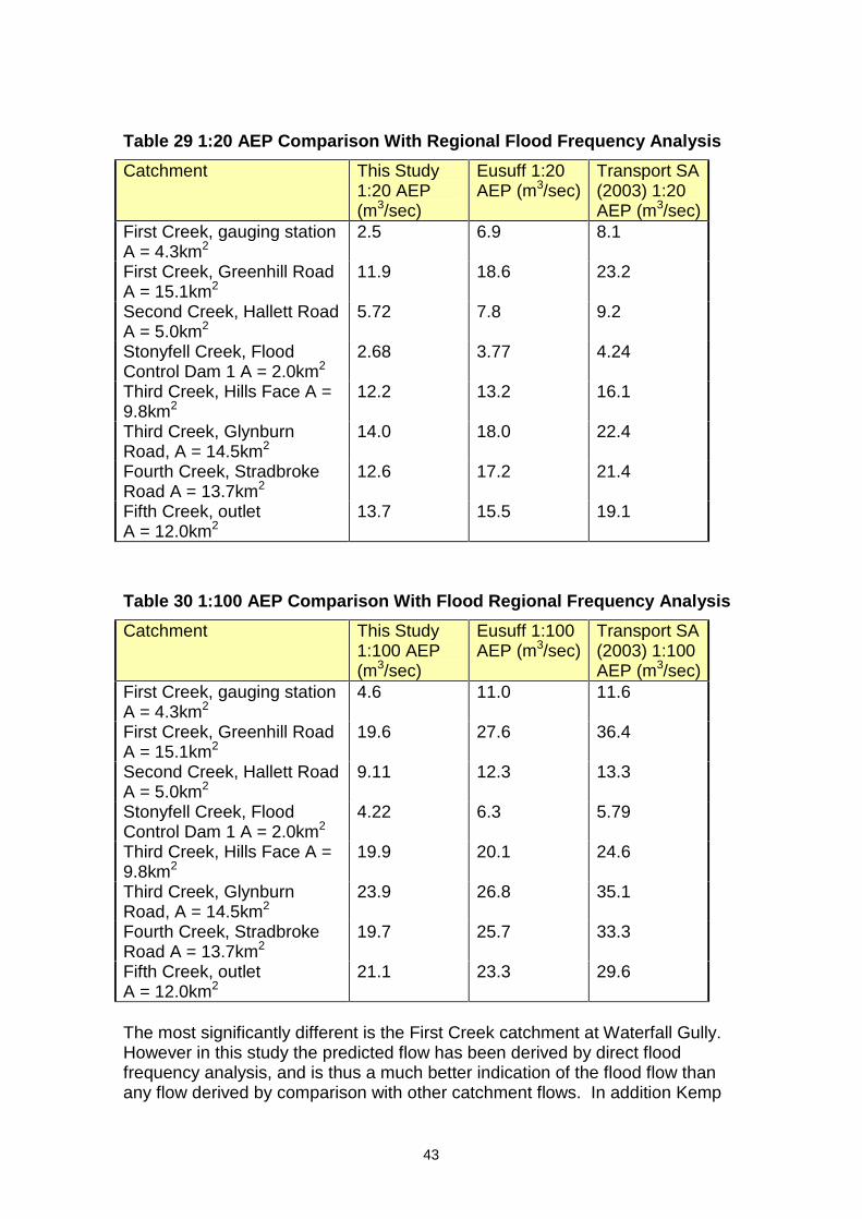
It can be seen that there are significant differences in the predicted flows from previous studies. However it is only in recent times that there has been an increase in the number of gauged catchments in the Mount Lofty Ranges that enables the proper assessment of parameter values. In addition there is in general another 20 year of data on which to base flood frequency analysis. The last study of First Creek (WBCM, 1985) had less than 10 years of gauging data, which is insufficient to carry out meaningful flood frequency analysis. The importance and value of collecting data can be seen in the above figures. The predicted rural flows can also be compared with other regional flood frequency analysis. Two appropriate studies are Eusuff (1995) for Mount lofty Ranges catchments and Transport SA (2003), for the Onkaparinga River catchment. Table 29 and Table 30 show the comparison for the 1:20 and 1:100 AEP flows. The predicted flows from this study are consistently less than the values derived in regional flood frequency analysis derived using other Mount Lofty Ranges catchments.

43

Table 29 1:20 AEP Comparison With Regional Flood Frequency Analysis

Catchment This Study 1:20 AEP (m3/sec)

Eusuff 1:20 AEP (m3/sec)

Transport SA (2003) 1:20 AEP (m3/sec)

First Creek, gauging station A = 4.3km2

2.5 6.9 8.1

First Creek, Greenhill Road A = 15.1km2

11.9 18.6 23.2

Second Creek, Hallett Road A = 5.0km2

5.72 7.8 9.2

Stonyfell Creek, Flood Control Dam 1 A = 2.0km2

2.68 3.77 4.24

Third Creek, Hills Face A = 9.8km2

12.2 13.2 16.1

Third Creek, Glynburn Road, A = 14.5km2

14.0 18.0 22.4

Fourth Creek, Stradbroke Road A = 13.7km2

12.6 17.2 21.4

Fifth Creek, outlet A = 12.0km2

13.7 15.5 19.1

Table 30 1:100 AEP Comparison With Flood Regional Frequency Analysis

Catchment This Study 1:100 AEP (m3/sec)

Eusuff 1:100 AEP (m3/sec)

Transport SA (2003) 1:100 AEP (m3/sec)


4.6 11.0 11.6


19.6 27.6 36.4


9.11 12.3 13.3


4.22 6.3 5.79


19.9

20.1 24.6

Third Creek, Glynburn Road, A = 14.5km2

23.9 26.8 35.1


19.7 25.7 33.3


21.1 23.3 29.6

The most significantly different is the First Creek catchment at Waterfall Gully. However in this study the predicted flow has been derived by direct flood frequency analysis, and is thus a much better indication of the flood flow than any flow derived by comparison with other catchment flows. In addition Kemp

44

(2002) and Kemp (2003) show that catchment lag as determined from calibrated RRR models is directly correlated with the percentage of catchment with native vegetation, and inversely correlated with catchment average slope. Higher catchment lag means more storage within the catchment, and thus lower peak flows. The hills face catchments have in general more native vegetation and steeper average slopes than other Mount Lofty Ranges catchments, and from the correlations can be expected to have lower flood flows for the same catchment area.

9 THE SIGNIFICANCE OF HISTORICAL FLOOD EVENTS The comparison of flows from the historical flood events in 1981 and 1983 indicates that in both cases the floods were well in excess of the predicted 1:100 AEP flow. The peak flow derived from flood marks on Fourth Creek in 1981 of 33m3/sec at Stradbroke Road is substantially greater than the predicted 1:100 AEP flow of 19.7m3/sec. However the catchment at the time was in a state that could in no way be considered to be average. The median API for the catchment is approximately 22.5mm, compared with the actual API at the commencement of the event of 151.2mm (the 99.8 percentile, or expected 1 day in 500). For a rainfall event of any frequency to produce a flood of the same frequency the catchment must be in �average� condition, as would be expected with an API close to 22.5mm. The probability of the rainfall was not significant (33.1mm in 4.5 hours, or less than 1:2 AEP). However this intensity is for all storms occurring during the year. If winter rainfall intensities only are examined, the rainfall event occurs much less frequently. BC Tonkin (1982) indicated that the rainfall intensity for the event was approximately 1:100 AEP for durations of 45 minutes to 3 hours if winter intensities only are considered. In summary the 1981 flood occurred on a very wet catchment, due to a rainfall event that was rare in terms of when it occurred. Because of the saturated nature of the catchment, losses were very low and direct surface runoff could occur, both of which meant a significantly higher peak flow than would occur normally with such a rainfall. It gives a warning that given relatively rare catchment conditions, extreme floods can result from only relatively minor rainfall events. The recorded peak flow at the Waterfall Gully gauging station in 1983 was 10.14m3/sec, well in excess of the predicted 1:100 AEP flow of 4.6m3/sec. The flood event occurred two weeks after a major bushfire in the area, which destroyed much of the understorey vegetation. In addition organic ground cover is converted to soluble ash giving rise to phenomena of water repellency

45

(Collings and Ball, 2003). Although the runoff depth was not large (3mm) the hydrograph showed a very short time of rise consistent with direct surface runoff, as would be expected with the lack of ground cover and potential water repellency. The direct surface runoff would not normally be a feature of the catchment, due to the amount of native vegetative cover. To assess the probability of the March 1983 flood in Waterfall Gully the combined probability of the fire and the storm rainfall must be examined. Unfortunately although the rainfall probability can be determined the annual risk of a substantial part of the catchment being affected by fire cannot. In the next few years it is expected that more work will be done to determine the level of fire risk in the Mount Lofty Ranges (Ayre, 2004). In addition to the annual risk, the rainfall must occur after the fire, and within the same season. The rainfall and fire can be considered to be independent, so if the probability of the rainfall in March 1983 was 10 to 1:20 AEP (5% to 10% in any year) probability and the fire 50 to 100 year (1% to 2% in any year), the probability of the 1983 flood was from 0.2% to 0.05% (500 to 2000 year ARI). This assumes that the bushfire will occur before the flood producing rain, so that actual probability of the March 1983 flood is less than this. What the 1983 flood tells us is that that any catchment that has been significantly affected by fire may produce floods well in excess of historically recorded floods.

10 PROBABLE MAXIMUM FLOOD HYDROGRAPHS An estimate of the probable maximum flood (PMF) is required for mapping. It was considered that the floodplain for the PMF would be relatively insensitive to the flow, and this fact together with the possibility of inflows from other catchments and the uncertainties in the prediction of the PMF led to the adoption of the simplified approach. It was decided to map a single event covering each catchment, and to assume a uniform rainfall distribution. The analysis of the River Sturt catchment (BC Tonkin, 1996) found that for catchments less than 100 km2 there is no need to calculate spatial variations in PMP for input into a rainfall � runoff model to derive PMF, since resulting increases in the PMF are minimal. PMP estimates for short duration storms (less than 3 hours) were derived using the procedures of the Bureau of Meteorology publication Bulletin 53 � �The Estimation of Probable Maximum Precipitation in Australia: Generalised Short-Duration Method�. The procedure was amended in accordance with the amendment published in December 1996. The catchment is considered to be rough, as all the catchment lies within 20km of terrain that can be considered to be rough. No elevation adjustment is

46

required. A moisture adjustment factor of 0.65 was adopted. Because of the size of the catchment durations of 1, 1.5, 2, 2.5 and 3 hours were assessed. The mean catchment rainfall depths were calculated as follows:

Table 31 First to Fifth Creek Short Duration PMP Estimates

Mean Depth (mm) Duration (hours) First

Creek (22.8km2)

Second Creek (18.7km2)

Third Creek (19.0km2)

Fourth Creek (23.0km2)

Fifth Creek (12.0km2)

1.0 285 289 289 285 296 1.5 364 370 370 364 380 2.0 426 432 432 426 447 2.5 471 478 478 471 491 3.0 521 520 520 521 536 The temporal patterns for the short duration storms were taken from Bulletin 53. For the conversion of PMP to a PMF the rainfall must be applied to the hydrological model, with an appropriate adjustment to losses to account for the low probability of the event. The procedure used to derive losses for the PMF was in accordance with Book 6 of Australian Rainfall & Runoff. Book 6 recommends the use of a continuing loss rather than proportional loss, on the basis of the interpretation of the proportional loss as the relative area of unsaturated proportion of the catchment to the total catchment. As storm magnitude increases the unsaturated proportion decreases, and thus proportional loss reduces. It is thus recommended in Book 6 that a small continuing loss (say 1mm/hr) be used instead for extreme events. A nominal baseflow is then added to obtain an estimate of the total flow. The difficulty in adopting this approach with the RRR model is that three processes are being modelled with a proportional loss model. It is difficult to see that processes 1 and 2 (related to baseflow and slow flow) will give an increasing contribution at extreme events. To follow the principles of Book 6 of Australian Rainfall and Runoff it would be more appropriate to assign a relatively large loss to processes 1 and 2, and a small loss to process 3. It is proposed initially to allow a proportional loss of 0.95 for processes 1 and 2, and 0.10 for process 3. The recommended initial loss is zero in all cases. For the urban area not directly connected to the gutter system (the unconnected area) it can be assumed that all rainfall appears as runoff, with the proportional loss being zero, as the recommended continuing loss of 1mm/hr will be negligible for the rainfall depths occurring during the PMP. It is thus proposed to use the following losses for PMF:

47

Table 32 PMF Losses for the RRR Model

Process Initial Loss (mm) Proportional Loss Rural process 1 0 0.95 Rural process 2 0 0.95 Rural process 3 0 0.10 Urban impervious 0 0 Urban unconnected 0 0 These flows can be compared with Nathan et al (1994), who devised a quick method for estimating PMF in south east Australia, relating flow to catchment area by the relationship Qp = 129.1A0.616.

Table 33 Comparison of PMF From This Study With Nathan (1994)

Catchment This Study PMF (m3/sec)

Nathan (1994) PMF (m3/sec)


200 317


614 687


263 348


137 198


428 527


662 647


701 597

The results show that there is general consistency with the Nathan regression. PMF values have not been given for catchments having substantial urban areas, as the hydrology model is not able to model the substantial floodplain flows, and associated storage.

11 HYDROGRAPHS FOR 1:500 AEP EVENTS In accordance with Book 6 of Australian Rainfall & Runoff flood events in excess of 1:100 AEP are termed rare events, and there are different requirements for design rainfalls and losses from large events (defined as 1:100 AEP or more frequent). For long duration rainfalls, which are critical on the upper catchments the use of the GSAM temporal patterns are recommended. In addition the use of regional rainfall frequency analysis (CRC-FORGE) is recommended where available.

48

This data is available in South Australia for storms in excess of 6 hours duration. The CRC-FORGE rainfalls were derived for the same sites as were used for the design rainfalls for events up to 1:100 AEP. The temporal patterns recommended for rare events are the GSDM (Generalised Short Duration Method, from Bureau of Meteorology, 1996) for events up to 12 hours duration, and the GSAM (Generalised Southern Australian Method) temporal patterns in excess of this. For this study the patterns used were from Bureau of Meteorology (1993). Storm losses must be adjusted to account for lower losses with rare events, and are interpolated between the losses for large events and the PMF losses. The interpolated design losses used for the 1:500 AEP are given in Table 34. It is assumed that the PMF has a nominal Annual Exceedance Probability of 1 x 107 years, in accordance with Book 6 of Australian Rainfall & Runoff.

Table 34 Losses for the 1:500 AEP Event

Process Initial Loss (mm) Proportional Loss

Rural process 1 - Brown Hill Creek 8.6 0.84 Rural process 2 - Brown Hill Creek 30.1 0.79 Rural process 3 - Brown Hill Creek 43.0 0.68 Rural process 1 - First Creek 0 0.70 Rural process 2 - First Creek 34.0 0.86 Rural process 3 - First Creek 86.0 0.75 Urban impervious 1 0 Urban unconnected 38.7 0.69 It was found that the critical duration for the 1:500 AEP events in the urban areas was less than 6 hours, and the rainfall intensities for these short duration events were derived in accordance with section 3.7 of Book 6, Australian Rainfall & Runoff. Hydrographs were calculated, and the flows for the probabilities plotted for all creeks to examine whether a smooth curve was evident. If this was not the case then the losses should be adjusted so that a smooth curve was formed. It was found that when plotting the curves that the rural catchments were satisfactory, but at the outlets to the River Torrens it was apparent that the 1:100 AEP flow fell below the curve formed by the other probability flows. Figure 16 shows First Creek as an example.

49

First Creek

1

10

100

1000

1E-070.0000010.000010.00010.0010.010.1

AEP

Q (

m^3

/sec

)

Waterfall

Outlet

Figure 16 Predicted Peak Flows in First Creek

To determine if it was the 1:100 AEP flow or the 1:500 AEP flow that needed adjustment the ratio of flows for the total catchment to the rural portion was calculated, as this should also form a smooth curve. It would also be expected that there would be a higher ratio for more frequent events, where the urban catchment can be expected to provide higher relative flows than the rural catchment. The increase in catchment peak flows due to urbanisation is well known.

Table 35 Ratio of Calculated Total Flow to Rural Flow (First Creek)

ARI (years) AEP Peak Flow at Waterfall (m3/sec)

Peak Flow at Outlet (m3/sec)

Ratio

20 0.05 2.5 21.2 8.4850 0.02 3.77 24.8 6.58

100 0.01 4.71 28.9 6.14500 0.002 8.77 60 6.84

PMF 0.0000001 201 954 4.75 It can be seen from Table 35 that it is the 1:500 AEP flow that does not fit the smooth curve, with a much higher flow expected. The loss for the pervious portion of the urban area was adjusted to try and smooth the curve. It was however found that there was not a significant change in the predicted peak flow. Indeed, using the unadjusted design loss was not sufficient to produce a good result.

50

The structure of the model was then considered. The model uses flood wave velocities through the urban area that are appropriate to the efficient channels, which are relatively straight and uniform compared with rural catchments, and often concrete lined. Velocities of 1.5 m/sec to 3m/sec were used in the model, and fitted the recorded hydrographs well. However flows in excess of the channel capacities will have a much lower flood wave velocity as they spread out across the floodplain. The model was adjusted so that flows in excess of the channel capacity (assumed to be 18m3/sec to 20 m3/sec) were directed to a parallel flow path with a flood wave velocity of 0.75m/sec, which is considered to be more typical of the probable velocity. This model showed considerably lower flows for 1:500 AEP and PMF.

First Creek

1

10

100

1000

0.00000010.000010.0010.1

AEP

Flo

w (

m^3

/sec

)Waterfall

Outlet

Table 36 First Creek Peak Flows With Adjusted Model

Table 37 Adjusted Model Peak Flows (First Creek)

ARI (years) AEP Peak Flow at Waterfall (m3/sec)

Peak Flow at Outlet (m3/sec)

Ratio

20 0.05 2.5 21.2 8.4850 0.02 3.77 24.8 6.58

100 0.01 4.71 28.9 6.14500 0.002 8.77 53.7 6.12

PMF 0.0000001 201 732 3.64

51

It can be seen now that the frequency curve for the total catchment is now more uniform, and follows the expected pattern of reducing difference between urban and rural flows with increasing event ARI. It indicates that the flows provided to the mapping consultant should only be used up to the channel capacity. Above this it is more appropriate to either use an adjusted model to account for the slower flow across the floodplain, or extract the hydrograph from the hydraulic model.

12 SUMMARY The RRR model has been used to predict flows throughout the catchments of First to Fifth Creeks. The model has been calibrated where possible, and the resulting parameter values used with design rainfalls to predict design flows at a number of locations. The values of the design flows have been checked where possible against at-station flood frequency analysis and historical storm events, to ensure consistency. In most cases the calibrated RRR model performs well. The prediction of design floods has been extended to rare (1:500 AEP) and extreme events, being the probable maximum flood (PMF).

13 REFERENCES Ayre, M. (2004), Manager Risk and Prevention, Emergency Services Administrative Unit, Department of Justice South Australia. Personal communication, 21/06/2004. BC Tonkin & Associates (1982) �Review of Second Creek Flood Mitigation Strategies� Report prepared for the Eastern Councils Drainage Board, January 1982. BC Tonkin & Associates (1982b) �Fourth Creek Flood Mitigation Study� Report prepared for the City of Campbelltown, July 1982. BC Tonkin & Associates (1982c) �First Creek Drainage Study� Report Prepared for the City of Kensington & Norwood, December 1982. BC Tonkin & Associates (1984) �Third Creek Floodplain Management Study� Report prepared for the City of Campbelltown, September 1984. BC Tonkin (1996)�River Sturt Flood Hydrology Study� Prepared for SA Water, August 1996. BOM (1993) �Generalised Probable Maximum Precipitation Estimates for the Kangaroo Creek and Mount Bold Catchments� Bureau of Meteorology hydrometeorological advisory service, HAS Report no: GSPMP/17, December 1993.

52

Bureau of Meteorology (1996) �The Estimation of Probable Maximum Precipitation in Australia: Generalised Short Duration Method� Bureau of Meteorology Bulletin 53, amended December 1996. Collings, G. and Ball, J. (2003) �The Hydrological Effects of the 1994 Wild Fire on the Royal national Park� IEAust. 28th Hydrology and Water Resources Symposium, Wollongong, November 2003. Eusuff, T.H. (1995)�A Regional Flood Frequency Approach to the Mount Lofty Ranges� Unpublished thesis, University of Adelaide, June 1995. Grubbs, F.E. and Beck, G. (1972) �Extension of sample sizes and percentage points for significance testing of outlying observations� Technometrics, Vol14, pp847-854. Hill, P., Mein, R. and Siriwardena, L. (1998) �How Much Rainfall Becomes Runoff � Loss Modelling for Flood Estimation� CRC for Catchment Hydrology, industry report 98/5, June 1998. Kemp, D.J and Lipp, W.R. �Predicting Storm Runoff in Adelaide � How Much do we Know� Hydrological Society of South Australia, Living With Water Seminar, Adelaide, October 1999. Kemp. D.J. (2002) �The Development of a Rainfall � Runoff � Routing (RRR) Model� Unpublished PhD thesis, University of Adelaide, August 2002. Kemp, D.J. (2003) �Finding the Hidden Factors of Catchment Lag � a Little Progress� I.E.Aust Hydrology and Water Resources Symposium, Wollongong, November 2003. Laurenson, E.M. (1964) "A Catchment Storage Model for Runoff Routing" Journal of Hydrology, Vol 2. pp141-163. Lower (1976) Calculations undertaken for the Eastern Councils Drainage Board by Mostyn Lower & Associates, June 1976. Nathan, R.J, Weinmann, P.E. and Gato, S.A. (1994) �A Quick Method for Estimating the Probable Maximum Flood for South East Australia� Water Down Under, Adelaide, I.E.Aust. National Conference Publication No.94/15. pp 229-234. Nordenson, T.J & Richards, M.M. �Hydrology of Flow Forecasting� in Ven Te Chow (editor-in-chief) �Handbook of Applied Hydrology� (1964) McGraw Hill Book Company, pp 25-102. Sinclair Knight Mertz (2000) �Application of CRC-FORGE Method to South Australia� Report produced for SA Water.

53

Transport SA (2003) "Hydrological Study of the Upper Onkaparinga River Catchment" Report produced for the Onkaparinga Catchment Water Management Board by Transport SA. Transport SA (2004) �Brown Hill Creek Hydrology Review Report� Report produced for the Patawalonga Catchment Water Management Board, as part of the Brown Hill � Keswick Creek Flood Mapping Study, February 2004. WBCM Consultants (1984) �South Eastern Suburbs of Adelaide; Stormwater Drainage Study�, August 1984. WBCM Consultants (1986) �First Creek Flood Plain Management Study� report produced for the City of Burnside, August 1986.

54

ADDENDUM : REVIEW OF THE HYDROLOOGY FOLLOWING THE NOVEMBER 2005 FLOOD

55

First to Fifth Creek Study Review of the Hydrology Following the November 2005 Flood David Kemp, DTEI The storm in November 2005 resulted in large flows in the First to Fifth Creek catchments, and these have been reviewed to determine if any changes to the predicted flows for floodplain mapping are required. Rainfall resulting from a north westerly airstream was highest in the higher parts of the Mount Lofty Ranges, with the long duration (24 to 48 hour) intensities having the lowest probability. The most significant was a recorded 130mm in 24 hours at Cherryville, having a probability between 1:50 and 1:100. By contrast the rainfall at Kent Town was 46mm in 24 hours, or between 1:1 and 1:2. This rainfall pattern meant that it was the rural parts of the catchments that had the lowest probability flows. The storm came at the end of a reasonably wet season. The daily API at Aldgate at 9am on 7 November was 63mm. Based on long term rainfall records this API is only exceeded on 10% to 15% of all days.

1 FIRST CREEK

1.1 Waterfall Gully The highest recorded flow in First Creek at the waterfall was 12.3m3/sec, but it was apparent from the inspection of the gauging station that the peak water level was well in excess of that predicted for this flow. Survey and hydraulic analysis by the Bureau of Meteorology initially resulted in an estimated peak flow of 20 m3/sec, with an error of potentially +/- 10 m3/sec. The level of flow at the weir below the waterfall indicated a flow of 15m3/sec, with a potential error of +/- 2m3/sec. These flows are well in excess of the predicted 100 year flow used in the mapping of 4.71m3/sec. The recorded hydrograph shows a very distinctive peak, with a drop in flow just before the peak occurred. Initial modelling was carried out with catchment parameters as used in the First to Fifth Creek study, and adjusting initial loss only. The loss parameters used for the study are given in Table 20. The initial loss for the process 1 (base flow) and process 2 (slow flow) was set at zero, and the fast flow was set at 50mm).

56

Table 38 Calibrated and Design RRR Model Design Loss Parameters � First Creek Catchment

IL2 (mm) IL3 (mm) PL1 PL2 PL3

Calibrated /

Estimated

39.52 n/a 0.66 0.84 0.75

Design 39.52 100 0.66 0.84 0.85

Figure 17 shows the result, with a good fit to the start of the hydrograph, and to the tail. The rainfall hyetograph at Mount Lofty is also shown.

Figure 17 First Creek at Waterfall - Adjusted Initial Loss Only

The predicted peak flow for the event from the model is 2.95 m3/sec, equivalent to between 1:20 and 1:50 AEP. Given that the catchment was relatively wet at the start of the event, this would be a reasonably expected outcome. As a next step the proportional loss for the fast runoff was reduced, so that at the time of peak flow there was 100% runoff. It can be seen in Figure 18 that the peak flow cannot be replicated, and that the apparent runoff volume is in excess of the rainfall. The hydrograph tail also does not match as well as the base case.

0

10

20

0.0

2.5

5.0

7.5

10.0

12.5

8 TueNov 2005

AW504517 [STORM 1]Max - Local (Catch 1)[0.000] Total Local Flow[0.000] Total Flow[2.947]

Rai

nfal

l [m

m/h

r]F

low

[cm

s]

Time

Total Rainfall (Catch 1) Total Flow Gauged Flow

57

Figure 18 First Creek at Waterfall - Total Runoff at Peak

This modelling indicated that the recorded hydrograph couldn�t be explained as a normal runoff event. A more detailed investigation of creek flows has since been carried out, with the survey and analysis by the Bureau of Meteorology determining flows in both tributaries at Chinaman�s hut, upstream of the gauging station. The high peak water level at the gauging station was thought to be a combination of a large peak flow, and local effects due to channel blockage at times during the flood event. The drop in recorded flow just before the peak is most likely to be as a result of inundation of the water level transducer. The estimated flow in the northern or Cleland branch is 10m3/sec, with a possible error of +/- 5m3/sec. The southern or Crafers branch had a flow of 5m3/sec, with a possible error of +/- 1m3/sec. The hydrological model was further sub-divided so that the flows in the two tributaries could be determined. It was found that with the initial loss of process 1 and 2 set to zero, the initial loss of process 3 set to 45mm, and the process 3 proportional loss set to match the tail of the hydrograph that the predicted flows were: Crafers Branch 3.0m3/sec Cleland Branch 2.1m3/sec Gauging Station 5.0m3/sec

0

10

20

0.0

2.5

5.0

7.5

10.0

12.5

8 TueNov 2005


Rai

nfal

l [m

m/h

r]F

low

[cm

s]

Time

Total Rainfall (Catch 1) Total Flow Gauged Flow

58

Following the flood Earth Tech were engaged to assess the nature and extent of debris flow in the catchment above the waterfall and to estimate the return period of the event. The report concluded that based on the size of material moved in the channel bed upstream of the gauging station that the flow would be in the range 6.5m3sec to 13m3sec. A flow of 13m3sec has been assumed in the analysis of predicted flood hydrographs. Figure 19 shows the detailed model result at the gauging station, with the hydrograph adjusted based on an assumed maximum flow of 13m3/sec. The hydrograph fit is good, apart from the time when the debris flow is assumed to be occurring.

0

10

20

0.0

2.5

5.0

7.5

10.0

12.5

8 TueNov 2005


Rai

nfal

l [m

m/h

r]F

low

[cm

s]

Time



Figure 19 First Creek at Waterfall - Detailed Model

1.2 Botanic Gardens The First Creek gauging station at the Botanic Gardens recorded a peak flow of 15.8m3/sec, but the high peak flow in Waterfall Gully may not be recorded at the Botanic Gardens, as overflows occur from the First Creek catchment to Greenhill Road, and the Parklands Creek in large events. The recorded peak flow is equivalent to a 10 � 20 year event.

59

05

1015

0.0

2.5

5.0

7.5

10.0

12.5

15.0

8 TueNov 2005


Rai

nfal

l [m

m/h

r]F

low

[cm

s]

Time



Figure 20 First Creek at Botanic Gardens

Modelling was carried out, and following calibration of the losses resulted in the hydrograph in Figure 20. The hyetograph shown is the Kent Town station. The initial rises in the hydrograph are due to the urban response. The assumed hydrograph at the waterfall, based on the gauged data was put into the model. It was found that the unconnected area (the balance of the urban catchment not the directly connected impervious area) was contributing flows, with an initial loss of 11.8mm, and a proportional loss of 0.76.

1.3 Implications The implication for the predicted flows for mapping in First Creek depends on the probability of debris flows from Wilson�s Bog, as these have a substantial effect on downstream flows. The highest recorded flow in the 29 years of recorded flows, if the 1983 and the 2005 floods are ignored, is 2.8m3/sec. The 1983 flood at the Waterfall Gully station was 10.1m3/sec, but this occurred immediately after a bushfire. In the study report the hydrograph was explained by direct surface runoff from part of the catchment, but the hydrograph shape is close to that of November 2005. Some debris flow may have occurred in 1983. The 2005 flood was caused in part by the failure of Wilson�s Bog. There are then three different flood mechanisms, the �normal� flows, the flood following bushfire, and the flood resulting from a failure of Wilsons Bog, and therefore three populations for the flood frequency. Of these three the 1983

60

and the 2005 floods are represented by only a single flood. No frequency analysis can thus be carried out on these. Instead it is proposed that a split distribution be used for the design floods, with the frequent floods (proposed to be less than 20 years ARI) being determined from normal flood frequency analysis, and the infrequent floods (1:50 AEP and greater) based on an assumed AEP for the 1983 and 2005 floods. From the 2005 flood it appeared that the flow was increased by 8 � 10 m3sec, the approximate peak of the 1983 flood. It is therefore proposed that the frequent event flood frequency be adjusted by this amount to provide the flood frequency adopted for the mapping update. The final flood peaks are given in Table 39, and are based on the flows calculated by the RRR model.

Table 39 Adjusted Design Flows at Waterfall

AEP Flow based on Flood Frequency Analysis (m3/sec)

Adjusted Design Peak Flow (m3/sec)

1:20 2.5 2.5 1:50 3.8 11.8 1:100 4.7 14.7 1:500 8.8 18.8 This would give an AEP for the 1983 flood of close to 1:50, and the 2005 flood of between 1:50 and 1:100. This is relatively consistent with the Earth Tech assessment that the 2005 flood did not exceed 1:50 AEP, based on the level of channel damage. To obtain long duration hydrographs for mapping a hydrograph due to the Wilsons Bog failure was derived by subtracting the predicted RRR model hydrograph from the assumed hydrograph, with a peak of 13m3/sec. This was then added to the design RRR model hydrograph. Only the hydrograph at the waterfall was updated.

61

Figure 21 Flood Frequency Analysis First Creek at Waterfall � With Split Distribution

2 SECOND CREEK The recorded peak flow at the gauging station in Stepney was 15.6m3/sec, which is equivalent to a flow of much less than 1:20 AEP (37.3m3/sec). Figure 22 shows the calibrated model hydrograph at Stepney, where the modelled flows match the recorded hydrograph reasonably well. The Burnside hyetograph is shown. The probability of the flow can be explained by the catchment having relatively little rural catchment. From the model the predicted flow at the Gandy Gully dam outlet was 3.2m3/sec, which is between 1:20 and 1:50 AEP, as would be expected from the catchment rainfall. Similarly the predicted flow at Slapes Gully Road is 6.3m3/sec, which is the same probability.

0.01

0.1

1

10

100

-3.5-3-2.5-2-1.5-1-0.500.511.522.5

Number of Standard Deviations

Dis

char

ge,

m^3

/s

Annual Exceedence Probability

0.99 0.98 0.95 0.9 0.8 0.7 0.6 0.5 0.4 0.3 0.2 0.1 0.05 0.02 0.01

62

010

20

0.0

2.5

5.0

7.5

10.0

12.5

15.0

8 TueNov 2005

9 Wed 10 Thu


Rai

nfal

l [m

m/h

r]F

low

[cm

s]

Time



Figure 22 Second Creek at Stepney

Mapping undertaken by Tonkin Consulting indicated that there should be considerable flows out of Stonyfell Creek at Hallett Road. Since this did not happen a cause was sought, and Tonkin Consulting found drawings of a flood control dam in Gandy Gully (flood control dam 1) that was not included in the original hydrology model. The model was updated following site confirmation of the dam drawings, which had been found in the Tonkin archives. The RRR model was then recalibrated with the dam in place, and updated design hydrographs produced for mapping. The effect of the inclusion of the dam on the flow at Hallett Road is given in Table 40.

Table 40 Effect of Flood Control Dam 1 in Gandy Gully on Stonyfell Creek Flows

ARI (years) No Flood Control Dam 1 (m3/sec)

With Flood Control dam 1 (m3/sec)

20 2.72 2.24 50 4.09 3.33 100 4.91 3.73

3 THIRD CREEK Third Creek was modelled, with the result of preliminary calibration shown in Figure 23. Although the start and end of the hydrographs could be well matched, there was a period in the middle of the storm that could not. The

63

initial part of the hydrograph was due to the urban response, and the end due to the rural response. The hydrograph shows a runoff from the pervious (unconnected) portion of the urban area, with an initial loss of 25mm, and a proportional loss of 0.85.

0102030

0.0

2.5

5.0

7.5

10.0

8 TueNov 2005

9 Wed


Rai

nfal

l [m

m/h

r]F

low

[cm

s]

Time



Figure 23 Third Creek at River Torrens

There is no indication from this storm event that the hydrology needs to be changed for Third Creek.

4 FOURTH CREEK The Fourth Creek gauging station at the Stradbroke School (BM023086) registered a peak flow of 8.8m3/sec, but the flow estimated from the flood marks at the site is 19m3/sec. The station failed during the event. Figure 24 shows the modelled and recorded flows, with the model losses adjusted to produce the estimated peak flow. The losses used are as follows: Sub-catchment IL1 (mm) Pl1 IL2 (mm) PL2 IL3 (mm) PL3

Morialta Conservation Park 0.0 0.66 5 0.5 50 0.85

Balance of Rural Area 0.0 0.82 5 0.5 50 0.85

Unfortunately, since the whole hydrograph was not recorded it is not possible to determine the exact loss regime. However the above losses are reasonable.

64

0102030

0.0

2.5

5.0

7.5

10.0

12.5

15.0

17.5

20.0

8 TueNov 2005

9 Wed

Forest [STORM 1]Max - Local (Catch 1)[0.000] Total Local Flow[0.000] Total Flow[19.734]

Rai

nfal

l [m

m/h

r]F

low

[cm

s]

Time



Figure 24 Fourth Creek at Stradbroke School

The estimated peak flow of 19m3/sec is of the order of 1:100 AEP (1:100 AEP flow at Stradbroke Road is 19.7m3/sec). Given the rainfalls in the upper catchment of Fourth Creek (around 50 years for 24 � 48 hours) and the state of the catchment (relatively wet) the flow is as expected, and no change in the predicted flows is considered necessary.

5 FIFTH CREEK The recorded peak flow at the Fifth Creek gauging station (BM023094) was 6.9m3/sec. However the actual peak level was greater than the peak recorded level, and the peak flow estimated from flood marks is 16m3/sec. This flow is approaching the predicted 1:50 AEP flow. Figure 25 shows a possible hydrograph, diverging only near the peak flow. The Black Hill hyetograph is shown. The following losses were used: Sub-catchment IL1 (mm) Pl1 IL2 (mm) PL2 IL3 (mm) PL3

Rural Area 0.0 0.82 0.0 0.86 40 0.60

These losses are reasonable, and the estimated peak flow of 16m3/sec is of the order of 1:50 AEP, as would be expected given the catchment condition and rainfall. No change to the predicted peak flows is considered necessary.

65

05

1015

0.0

2.5

5.0

7.5

10.0

12.5

15.0

8 TueNov 2005

9 Wed


Rai

nfal

l [m

m/h

r]F

low

[cm

s]

Time



Figure 25 Fifth Creek at Athelstone

6 SUMMARY The review following the November 2005 flood has shown the need to amend the design hydrographs for First and Second (Stonyfell) Creek. In the case of First Creek it is as a result of the discovery of the chance that Wilsons Bog can fail, raising downstream flows to well in excess of those that would normally occur. Following mapping of the Stonyfell Creek flood predicted from the model it was found that a flood control basin existed in Gandy Gully, and that it had not been included in the model. Plans of the basin have subsequently been found, and the hydrographs for mapping have been updated.

66

APPENDIX 1 CATCHMENT PLAN

APPENDIX 2 CALIBRATION HYDROGRAPHS

First Creek � Gauging Station (AW504517)

First Creek 30/08/86

0.0

0.2

0.4

0.6

0.8

1.0

1.2

0 50 100 150

Time (hrs)

Flo

w (

m^

3/se

c)

Measured value

Calculated value


0.0

0.1

0.2

0.3

0.4

0.5

0.6

0.7

0 50 100 150

Time (hrs)

Flo

w (

m^

3/se

c)

Measured value

Calculated value


0.0

0.1

0.2

0.3

0.4

0.5

0.6

0.7

0.8

0.9

0 50 100 150

Time (hrs)

Flo

w (

m^

3/se

c)

Measured value

Calculated value


0.0

0.1

0.2

0.3

0.4

0.5

0.6

0.7

0.8

0 50 100 150 200Time (hrs)

Flo

w (

m^

3/se

c)

Measured value

Calculated value


0.00

0.10

0.20

0.30

0.40

0.50

0.60

0.70

0.80

0 50 100 150

Time (hrs)

Flo

w (

m^

3/se

c)

Measured value

Calculated value


0.0

0.1

0.2

0.3

0.4

0.5

0.6

0.7

0 50 100 150

Time (hrs)

Flo

w (

m^

3/se

c)

Measured value

Calculated value


0.0

0.1

0.2

0.3

0.4

0.5

0.6

0.7

0.8

0.9

0 50 100 150

Time (hrs)

Flo

w (

m^

3/se

c)

Measured value

Calculated value

First Creek � Botanic Gardens AW504578

050

100

0.0

2.5

5.0

7.5

10.0

12PM6 Thu Feb 97

3PM 6PM 9PM


Rai

nfal

l [m

m/h

r]F

low

[cm

s]

Time



050

100

0.0

2.5

5.0

7.5

10.0

12.5

6 TueOct 98


Rai

nfal

l [m

m/h

r]F

low

[cm

s]

Time



050

100

0.0

2.5

5.0

7.5

10.0

12.5

15.0

17.5

20.0

22.5

6PM22 Sat May 99

9PM 23 Sun 3AM 6AM


Rai

nfal

l [m

m/h

r]F

low

[cm

s]

Time



050

100

0.0

2.5

5.0

7.5

10.0

16 TueMay 2000


Rai

nfal

l [m

m/h

r]F

low

[cm

s]

Time



0255075

0.0

2.5

5.0

7.5

10.0

12.5

15.0

6 WedJun 2001

7 Thu


Rai

nfal

l [m

m/h

r]F

low

[cm

s]

Time



050

100

0.0

2.5

5.0

7.5

10.0

12PM6 Fri Jun 2003

3PM 6PM 9PM


Rai

nfal

l [m

m/h

r]F

low

[cm

s]

Time



0255075

0.0

0.5

1.0

1.5

2.0

2.5

3.0

3.5

4.0

4.5

31 FriOct 2003

1 Nov


Rai

nfal

l [m

m/h

r]F

low

[cm

s]

Time



Second Creek at Stepney BM023104

010

20

0.0

2.5

5.0

7.5

10.0

12.5

15.0

27 FriJun 2003

28 Sat


Rain

fall [

mm

/hr]

Flow

[cm

s]

Time



0

5

10

0

1

2

3

4

5

6

7

8

9

25 FriJul 2003

3AM 6AM


Rai

nfal

l [m

m/h

r]F

low

[cm

s]

Time



010

20

0.0

2.5

5.0

7.5

10.0

5 TueAug 2003

6 Wed


Rai

nfal

l [m

m/h

r]Fl

ow [c

ms]

Time



05

1015

0

1

2

3

4

5

6

7

23 SatAug 2003

24 Sun 25 Mon


Rai

nfal

l [m

m/h

r]F

low

[cm

s]

Time



010

20

0

1

2

3

4

5

6

7

8

6PM30 Thu Oct 2003

9PM 31 Fri 3AM 6AM 9AM 12PM


Rai

nfal

l [m

m/h

r]Fl

ow [c

ms]

Time



Third Creek at Forsyth Grove AW504579

010

20

0

1

2

3

4

5

6

7

19 SunMay 2002


Rai

nfal

l [m

m/h

r]Fl

ow [c

ms]

Time



0

10

20

0

1

2

3

4

6AM27 Thu Jun 2002

9AM 12PM 3PM 6PM 9PM


Rai

nfal

l [m

m/h

r]F

low

[cm

s]

Time



0

25

50

0.0

2.5

5.0

7.5

12PM25 Mon Nov 2002

3PM 6PM 9PM 26 Tue 3AM


Rai

nfal

l [m

m/h

r]F

low

[cm

s]

Time



0

20

40

0

1

2

3

4

5

6

31 FriOct 2003


Rai

nfal

l [m

m/h

r]F

low

[cm

s]

Time



05

1015

0.00

0.25

0.50

0.75

1.00

1.25

1.50

1.75

2.00

9PM1 Sat Nov 2003

10PM 11PM 2 Sun 1AM


Rai

nfal

l [m

m/h

r]F

low

[cm

s]

Time



0.02.55.07.5

0.00

0.25

0.50

0.75

1.00

1.25

1.50

9PM19 Fri Dec 2003

20 Sat 3AM


Rai

nfal

l [m

m/h

r]F

low

[cm

s]

Time



010

20

0.0

0.5

1.0

1.5

2.0

2.5

3.0

3.5

4.0

4.5

9AM21 Sun Dec 2003

12PM 3PM


Rai

nfal

l [m

m/h

r]F

low

[cm

s]

Time



0.02.55.07.5

0.00

0.25

0.50

0.75

1.00

1.25

1.50

9PM19 Fri Dec 2003

20 Sat 3AM


Rai

nfal

l [m

m/h

r]F

low

[cm

s]

Time



010

20

0.0

0.5

1.0

1.5

2.0

2.5

3.0

18 TueMay 2004


Rai

nfal

l [m

m/h

r]F

low

[cm

s]

Time



0

10

20

0.0

0.5

1.0

1.5

2.0

2.5

3PM28 Fri May 2004

4PM 5PM 6PM 7PM 8PM


Rai

nfal

l [m

m/h

r]F

low

[cm

s]

Time



Fifth Creek at Athelstone BM023094

0102030

0.00

0.25

0.50

0.75

1.00

1.25

1.50

1.75

2.00

12PM30 Wed Apr 2003

3PM 6PM 9PM 1 May 3AM


Rai

nfal

l [m

m/h

r]F

low

[cm

s]

Time



010

20

0.00

0.25

0.50

0.75

1.00

1.25

1.50

1.75

2.00

2.25

12PM23 Fri May 2003

3PM 6PM 9PM 24 Sat


Rai

nfal

l [m

m/h

r]F

low

[cm

s]

Time



010

20

0.00

0.25

0.50

0.75

1.00

1.25

1.50

1.75

27 FriJun 2003


Rai

nfal

l [m

m/h

r]F

low

[cm

s]

Time



05

10

0.00

0.25

0.50

0.75

1.00

1.25

6AM21 Sun Dec 2003

9AM 12PM 3PM 6PM


Rai

nfal

l [m

m/h

r]F

low

[cm

s]

Time



Sixth Creek AW504523

Sixth Creek 21/06/87

0

5

10

15

20

25

30

0 20 40 60 80 100 120Time (hrs)

Flo

w (

m^

3/se

c)

Measured value

Calculated value


0

5

10

15

20

25

30

0 20 40 60 80 100 120Time (hrs)

Flo

w (

m^3

/sec

)

Measured value

Calculated value


0

10

20

30

40

50

60

70

80

0 50 100

Time (hrs)

Flo

w (

m^

3/se

c)

Measured value

Calculated value


0

5

10

15

20

25

30

0 50 100Time (hrs)

Flo

w (

m^

3/se

c) Measured value

Calculated value


0

2

4

6

8

1012

14

16

18

20

0 50 100

Time (hrs)

Flo

w (

m^

3/se

c)

Measured value

Calculated value


0

2

4

6

8

10

12

14

16

18

0 50 100Time (hrs)

Flo

w (

m^

3/se

c)

Measured value

Calculated value

APPENDIX 3 REPRESENTATIVE TOTAL RAINFALLS

Adelaide (Kent Town) Total rainfall in millimetres 1:1 1:2 1:5 1:10 1:20 1:50 1:100 1:200 1:500

5m 3.6 4.8 6.7 8.1 10.1 12.9 15.5 18.3 22.7

6m 4.0 5.4 7.5 9.1 11.2 14.4 17.2 20.4 25.2

8m 4.7 6.4 8.9 10.7 13.2 16.9 20.2 23.9 29.5

10m 5.4 7.2 10.0 12.1 14.8 19.0 22.6 26.8 33.1

12m 5.9 8.0 11.0 13.2 16.3 20.8 24.8 29.3 36.1

14m 6.4 8.6 11.9 14.3 17.5 22.4 26.7 31.4 38.8

15m 6.6 8.9 12.3 14.7 18.1 23.1 27.5 32.4 40.0

16m 6.8 9.2 12.7 15.2 18.6 23.8 28.3 33.4 41.1

18m 7.2 9.7 13.4 16.0 19.7 25.1 29.8 35.1 43.2

20m 7.6 10.2 14.0 16.8 20.6 26.3 31.2 36.7 45.2

22m 8.0 10.7 14.6 17.5 21.5 27.4 32.4 38.2 46.9

24m 8.3 11.1 15.2 18.2 22.3 28.3 33.6 39.5 48.5

25m 8.4 11.3 15.5 18.5 22.6 28.8 34.2 40.2 49.3

26m 8.6 11.5 15.7 18.8 23.0 29.3 34.7 40.8 50.1

28m 8.9 11.9 16.2 19.4 23.7 30.1 35.7 42.0 51.5

30m 9.1 12.2 16.7 19.9 24.4 31.0 36.7 43.1 52.8

32m 9.4 12.6 17.1 20.5 25.0 31.7 37.5 44.1 54.0

34m 9.6 12.9 17.6 20.9 25.6 32.5 38.4 45.1 55.2

36m 9.8 13.2 18.0 21.4 26.1 33.1 39.2 46.0 56.3

38m 10.1 13.5 18.3 21.9 26.6 33.8 40.0 46.9 57.4

40m 10.3 13.7 18.7 22.3 27.2 34.4 40.7 47.7 58.4

45m 10.8 14.4 19.6 23.3 28.3 35.9 42.4 49.7 60.7

50m 11.2 15.0 20.3 24.2 29.4 37.2 43.9 51.5 62.8

55m 11.6 15.5 21.1 25.0 30.4 38.4 45.3 53.1 64.8

60m 12.0 16.1 21.7 25.8 31.3 39.6 46.6 54.6 66.5

65m 12.4 16.6 22.4 26.5 32.2 40.7 47.9 56.0 68.2

70m 12.8 17.1 23.0 27.3 33.1 41.7 49.1 57.4 69.8

75m 13.2 17.5 23.6 27.9 33.9 42.7 50.2 58.6 71.3

80m 13.5 18.0 24.2 28.6 34.6 43.6 51.3 59.8 72.7

90m 14.1 18.8 25.2 29.8 36.0 45.3 53.2 62.1 75.4

105m 15.0 19.9 26.6 31.4 37.9 47.6 55.9 65.0 78.9

120m 15.8 20.9 27.9 32.9 39.7 49.7 58.2 67.7 82.0

135m 16.5 21.8 29.1 34.2 41.2 51.5 60.3 70.1 84.8

150m 17.1 22.7 30.2 35.4 42.6 53.3 62.3 72.4 87.4

3hr 18.3 24.3 32.1 37.6 45.2 56.4 65.8 76.3 92.0

3.5hr 19.4 25.6 33.9 39.6 47.5 59.1 69.0 79.9 96.1

Adelaide (Kent Town) continued Total rainfall in millimetres 1:1 1:2 1:5 1:10 1:20 1:50 1:100 1:200 1:500

4hr 20.4 26.9 35.4 41.4 49.6 61.6 71.8 83.0 99.8

5hr 22.2 29.2 38.3 44.6 53.3 66.0 76.8 88.6 106.3

6hr 23.7 31.2 40.8 47.4 56.5 69.9 81.1 93.5 111.9

7hr 25.2 33.0 43.0 49.9 59.4 73.3 85.0 97.8 116.9

8hr 26.4 34.7 45.0 52.2 62.1 76.4 88.5 101.8 121.4

9hr 27.6 36.2 46.9 54.3 64.5 79.3 91.7 105.4 125.6

10hr 28.7 37.6 48.6 56.2 66.7 82.0 94.7 108.7 129.4

11hr 29.8 39.0 50.3 58.1 68.8 84.4 97.5 111.8 133.0

12hr 30.8 40.2 51.8 59.8 70.8 86.8 100.1 114.8 136.4

13hr 31.5 41.1 53.0 61.1 72.3 88.6 102.2 117.1 139.2

14hr 32.1 41.9 54.0 62.3 73.7 90.3 104.2 119.4 141.8

15hr 32.7 42.7 55.0 63.4 75.1 91.9 106.0 121.5 144.3

16hr 33.3 43.5 56.0 64.5 76.3 93.5 107.8 123.5 146.6

17hr 33.8 44.2 56.8 65.5 77.5 94.9 109.4 125.4 148.9

18hr 34.4 44.9 57.7 66.5 78.7 96.3 111.0 127.2 151.0

19hr 34.9 45.5 58.5 67.4 79.8 97.6 112.5 128.9 153.0

20hr 35.3 46.1 59.3 68.3 80.8 98.9 114.0 130.5 154.9

21hr 35.8 46.7 60.0 69.2 81.8 100.1 115.4 132.1 156.8

22hr 36.2 47.3 60.8 70.0 82.8 101.2 116.7 133.6 158.5

23hr 36.6 47.8 61.4 70.8 83.7 102.4 117.9 135.0 160.2

24hr 37.0 48.4 62.1 71.5 84.6 103.4 119.2 136.4 161.8

27hr 35.3 46.1 59.2 68.1 80.5 98.5 113.4 129.8 154.0

30hr 39.2 51.1 65.5 75.4 89.1 108.9 125.5 143.6 170.2

33hr 40.0 52.2 67.0 77.0 91.1 111.2 128.1 146.6 173.7

36hr 40.8 53.3 68.3 78.5 92.8 113.3 130.5 149.2 176.9

39hr 41.6 54.2 69.4 79.8 94.3 115.2 132.6 151.6 179.7

42hr 42.2 55.0 70.5 81.0 95.7 116.8 134.5 153.8 182.2

45hr 42.8 55.8 71.4 82.1 96.9 118.3 136.2 155.7 184.4

48hr 43.3 56.5 72.3 83.0 98.0 119.7 137.7 157.4 186.4

51hr 43.8 57.1 73.0 83.9 99.0 120.9 139.0 158.9 188.2

54hr 44.2 57.6 73.7 84.7 99.9 121.9 140.3 160.3 189.8

57hr 44.6 58.1 74.3 85.4 100.7 122.9 141.3 161.5 191.2

60hr 44.9 58.5 74.9 86.0 101.4 123.7 142.3 162.6 192.4

63hr 45.2 58.9 75.4 86.5 102.1 124.5 143.1 163.5 193.5

66hr 45.5 59.3 75.8 87.0 102.6 125.1 143.9 164.4 194.5

69hr 45.8 59.6 76.2 87.4 103.1 125.7 144.5 165.1 195.3

72hr 46.0 59.9 76.5 87.8 103.5 126.2 145.1 165.7 196.0

Norton Summit Total rainfall in millimetres 1:1 1:2 1:5 1:10 1:20 1:50 1:100 1:200 1:500

5m 4.4 5.7 7.5 8.6 10.3 12.6 14.6 16.7 19.9

6m 4.9 6.4 8.3 9.6 11.4 14.0 16.2 18.6 22.1

8m 5.8 7.6 9.8 11.4 13.5 16.5 19.0 21.7 25.8

10m 6.6 8.6 11.1 12.8 15.1 18.5 21.3 24.4 28.9

12m 7.3 9.5 12.2 14.1 16.6 20.3 23.3 26.6 31.5

14m 7.9 10.3 13.2 15.2 17.9 21.8 25.1 28.6 33.8

15m 8.2 10.6 13.7 15.7 18.5 22.5 25.9 29.5 34.9

16m 8.4 11.0 14.1 16.2 19.1 23.2 26.6 30.4 35.9

18m 8.9 11.6 14.9 17.1 20.1 24.5 28.1 32.0 37.7

20m 9.4 12.2 15.6 17.9 21.1 25.6 29.3 33.4 39.4

22m 9.8 12.8 16.3 18.7 22.0 26.6 30.5 34.7 40.9

24m 10.2 13.3 16.9 19.4 22.8 27.6 31.6 36.0 42.3

25m 10.4 13.6 17.2 19.7 23.2 28.1 32.1 36.5 43.0

26m 10.6 13.8 17.5 20.0 23.5 28.5 32.6 37.1 43.6

28m 11.0 14.3 18.1 20.7 24.3 29.4 33.6 38.2 44.8

30m 11.3 14.7 18.6 21.3 24.9 30.2 34.5 39.1 46.0

32m 11.6 15.1 19.1 21.8 25.6 30.9 35.3 40.1 47.0

34m 12.0 15.5 19.6 22.3 26.2 31.6 36.1 41.0 48.0

36m 12.2 15.9 20.1 22.8 26.7 32.3 36.9 41.8 49.0

38m 12.5 16.2 20.5 23.3 27.3 32.9 37.6 42.6 49.9

40m 12.8 16.6 20.9 23.8 27.8 33.6 38.3 43.4 50.8

45m 13.4 17.4 21.9 24.9 29.0 35.0 39.9 45.1 52.8

50m 14.0 18.1 22.8 25.8 30.2 36.3 41.3 46.7 54.6

55m 14.5 18.8 23.6 26.7 31.2 37.5 42.6 48.2 56.3

60m 15.1 19.4 24.3 27.6 32.1 38.6 43.8 49.5 57.8

65m 15.6 20.1 25.2 28.5 33.2 39.8 45.3 51.1 59.6

70m 16.1 20.7 25.9 29.4 34.2 41.0 46.6 52.7 61.4

75m 16.5 21.3 26.7 30.2 35.2 42.2 47.9 54.1 63.0

80m 17.0 21.9 27.4 31.0 36.1 43.3 49.1 55.5 64.6

90m 17.8 23.0 28.7 32.5 37.8 45.3 51.4 58.0 67.6

105m 19.0 24.5 30.5 34.5 40.1 48.1 54.6 61.5 71.6

120m 20.1 25.8 32.2 36.4 42.3 50.6 57.4 64.7 75.3

135m 21.0 27.1 33.7 38.1 44.2 52.9 60.0 67.6 78.7

150m 21.9 28.2 35.1 39.6 46.0 55.1 62.4 70.3 81.8

3hr 23.6 30.3 37.7 42.5 49.4 59.0 66.8 75.2 87.4

3.5hr 25.1 32.2 40.0 45.1 52.3 62.5 70.8 79.6 92.5

Norton Summit (continued) Total rainfall in millimetres 1:1 1:2 1:5 1:10 1:20 1:50 1:100 1:200 1:500

4hr 26.4 34.0 42.1 47.5 55.0 65.7 74.4 83.7 97.1

5hr 28.9 37.1 45.9 51.7 59.9 71.4 80.8 90.8 105.3

6hr 31.1 39.9 49.3 55.5 64.2 76.5 86.5 97.2 112.6

7hr 33.0 42.4 52.4 58.9 68.1 81.0 91.6 102.9 119.1

8hr 34.9 44.7 55.2 62.0 71.6 85.2 96.3 108.1 125.1

9hr 36.5 46.8 57.8 64.8 75.0 89.1 100.6 113.0 130.7

10hr 38.1 48.9 60.2 67.5 78.0 92.7 104.7 117.5 135.9

11hr 39.6 50.7 62.5 70.1 80.9 96.1 108.5 121.7 140.7

12hr 41.0 52.5 64.6 72.5 83.7 99.4 112.1 125.7 145.3

13hr 42.1 54.0 66.6 74.7 86.3 102.6 115.9 130.0 150.4

14hr 43.2 55.4 68.4 76.9 88.9 105.7 119.5 134.1 155.3

15hr 44.2 56.8 70.2 78.9 91.3 108.7 122.9 138.1 160.0

16hr 45.2 58.1 71.9 80.8 93.6 111.6 126.2 141.9 164.4

17hr 46.2 59.3 73.5 82.7 95.9 114.3 129.4 145.5 168.8

18hr 47.1 60.5 75.0 84.5 98.0 117.0 132.4 149.0 172.9

19hr 47.9 61.6 76.5 86.2 100.1 119.5 135.4 152.4 177.0

20hr 48.7 62.7 77.9 87.9 102.1 121.9 138.2 155.6 180.8

21hr 49.5 63.7 79.3 89.5 104.0 124.3 140.9 158.8 184.6

22hr 50.3 64.7 80.6 91.1 105.8 126.6 143.6 161.9 188.3

23hr 51.0 65.7 81.9 92.6 107.6 128.8 146.2 164.8 191.8

24hr 51.7 66.7 83.2 94.0 109.4 131.0 148.7 167.7 195.2

27hr 49.7 64.2 80.3 90.9 105.8 126.9 144.2 162.8 189.8

30hr 55.5 71.7 89.9 101.9 118.8 142.7 162.3 183.4 214.0

33hr 57.2 73.9 92.8 105.3 122.9 147.8 168.3 190.3 222.3

36hr 58.7 75.9 95.5 108.5 126.7 152.6 173.8 196.8 230.1

39hr 60.1 77.7 98.0 111.4 130.3 157.0 179.0 202.8 237.4

42hr 61.3 79.4 100.3 114.2 133.6 161.2 183.9 208.4 244.1

45hr 62.5 81.0 102.4 116.7 136.7 165.0 188.4 213.7 250.5

48hr 63.6 82.4 104.4 119.0 139.5 168.6 192.6 218.6 256.5

51hr 64.6 83.7 106.2 121.2 142.2 172.0 196.6 223.3 262.1

54hr 65.5 85.0 107.9 123.3 144.7 175.2 200.4 227.6 267.4

57hr 66.3 86.1 109.5 125.2 147.0 178.2 203.9 231.7 272.4

60hr 67.1 87.2 111.0 127.0 149.2 180.9 207.2 235.6 277.1

63hr 67.8 88.2 112.4 128.7 151.3 183.6 210.3 239.3 281.6

66hr 68.5 89.1 113.7 130.2 153.2 186.0 213.2 242.7 285.8

69hr 69.1 89.9 114.9 131.7 155.0 188.3 215.9 245.9 289.8

72hr 69.7 90.7 116.0 133.0 156.7 190.5 218.5 249.0 293.5

APPENDIX 4 CRC-FORGE RAINFALLS

Adelaide Longitude 138.59 Latitude -34.92 Duration 1:50 1:100 1:200 1:500 1:1000 1:2000

6 69.6 81.8 96.4 120.8 143.9 172 9 79.2 93 109.7 137.4 163.7 195.7

12 86.8 102 120.3 150.6 179.4 214.5 18 96.3 113.1 133.4 167.1 199.1 238 24 107.7 126.5 149.2 186.9 222.7 266.2 30 112.9 132.6 156.4 196 233.8 280.2 36 117.3 137.7 162.5 203.8 243.4 292.2 48 124.5 146.2 172.6 216.7 259.2 312.2 60 130.2 152.4 179.6 225.1 269 323.8 72 135.1 157.7 185.6 232.2 277.2 333.5 96 140.7 164.3 192.7 240.4 286.5 344

120 144.3 168.5 197.2 245.6 292.2 350.2 Payneham Longitude 138.65 Latitude -34.92 Duration 1:50 1:100 1:200 1:500 1:1000 1:2000

6 72 84.5 99.8 125.3 149.7 179.7 9 82.8 97.2 114.7 144.1 172.2 206.7

12 91.4 107.3 126.7 159.1 190.1 228.2 18 102.6 120.4 142.2 178.6 213.4 256.1 24 114.1 134 158.2 198.6 237.3 284.9 30 120.2 141 166.4 208.9 249.6 299.8 36 125.3 147 173.5 217.8 260.1 312.5 48 133.9 157 185.3 232.4 277.5 333.7 60 140.7 164.5 193.8 242.7 289.6 348.6 72 146.4 170.9 201 251.5 299.9 361.3 96 153.3 178.9 209.9 262.2 312.4 376.6

120 157.8 184.2 215.7 269 320.4 386.4 Campbelltown Longitude 138.67 Latitude -34.89 Duration 1:50 1:100 1:200 1:500 1:1000 1:2000

6 71.4 83.8 98.9 124.3 148.5 178.3 9 81 95.1 112.2 141 168.5 202.3

12 89.5 105 124 155.8 186.2 223.5 18 100.3 117.7 139 174.6 208.6 250.5 24 115.7 135.8 160.4 201.4 240.7 289 30 122.1 143.2 169 212.2 253.5 304.2 36 127.5 149.5 176.4 221.5 264.5 317.2 48 136.6 160.1 188.8 236.9 282.7 338.9 60 143.7 168 197.9 248 295.7 355.1 72 149.7 174.8 205.6 257.4 306.9 368.9 96 157 183.3 215.2 269 320.5 386

120 161.9 189 221.5 276.5 329.4 397.2

Norton Summit Longitude 138.73 Latitude -34.92 Duration 1:50 1:100 1:200 1:500 1:1000 1:2000

6 76.2 89.5 105.9 133.3 159.6 192 9 89.1 104.7 123.8 155.9 186.6 224.5

12 99.6 117 138.4 174.2 208.6 250.9 18 117 137.4 162.5 204.7 245.1 294.8 24 127.8 150.1 177.5 223.5 267.7 321.9 30 137.4 161.5 191.1 240.8 288.6 347.9 36 145.8 171.4 202.9 255.9 307 370.6 48 160.2 188.4 223.1 281.7 338.3 409.6 60 171.5 201.2 237.8 299.8 359.8 435.5 72 181.4 212.3 250.5 315.5 378.4 457.8 96 193.5 226.5 266.6 335 401.3 485

120 201.6 236 277.3 347.8 416.2 502.4 Eagle on the Hill Longitude 138.67 Latitude -34.98 Duration 1:50 1:100 1:200 1:500 1:1000 1:2000

6 80.4 94.5 112 141.7 170.5 206.4 9 94.5 111.1 131.6 166.5 200.4 242.6

12 106.6 125.3 148.4 187.9 226.1 273.6 18 124.2 146 173 218.9 263.4 318.8 24 134.5 158.1 187.3 237.1 285.3 345.3 30 143.5 168.7 200 253.4 305.4 370.3 36 151.2 177.9 211 267.5 322.7 391.9 48 164.2 193.4 229.6 291.5 352.2 428.8 60 175.5 206 244 309 373 453.1 72 185.2 216.9 256.5 324.2 390.8 473.9 96 197.3 231.2 272.4 343.1 412.6 498.5

120 205.6 240.8 283 355.4 426.7 514

APPENDIX 5 Summary of Flows (updated following November 2005 flood) This appendix contains a summary of the flows in the creeks at points along the channel derived from the hydrology model. The hydrology model assumes that all flow is contained within the channel. If the flow is greater than the capacity of the channel the flow will be overestimated. For this reason only flows up to 1:100 AEP are given here, as flows in excess of 1:100 AEP will be impacted significantly by floodplain storage. First Creek Location 1:20 AEP

(m3/sec) 1:50 AEP (m3/sec)

1:100 AEP (m3/sec)

Waterfall 2.50 11.8 14.7 Hills face zone boundary

11.0 14.7 18.3

Glynburn Road 11.4 15.9 19.7 Tusmore Park 12.5 16.7 20.4 Portrush Road 12.8 17.0 20.7 Osmond Tce. 13.2 17.7 21.4 North Tce. 14.1 19.3 23.2 Frome Road 17.2 23.6 28.5 Botanic Creek Location 1:20 AEP*

(m3/sec) 1:50 AEP* (m3/sec)

1:100 AEP* (m3/sec)

Bartels Road 3.4 3.6 3.7 Botanic Road 4.1 5.4 6.2 *Note: these flows are from hydraulic model � storage in parklands is not well defined in hydrology model Second Creek Location 1:20 AEP


1:100 AEP (m3/sec)

Slapes Gully Road 5.37 7.12 8.61 Hallett Road 5.72 7.56 9.11 Lockwood Road 6.46 9.45 10.1 Glynburn Road 9.59 11.2 13.1 Tusmore Ave 13.0 15.6 18.3 The Parade 18.5 22.3 25.8 Magill Road 37.3 43.2 47.7 Outlet 44.3 52.0 55.5

Stonyfell Creek Location 1:20 AEP


1:100 AEP (m3/sec)

Gandy Gully dam outlet

2.02 2.62 2.96

Hallett Road 2.24 3.33 3.73 Kensington flood control dam inlet

9.45 11.0 12.5

The Parade 6.71 7.13 8.47 Portrush Rd 16.7 18.7 19.8 Third Creek Location 1:20 AEP


1:100 AEP (m3/sec)

Norton Summit Road

12.2 16.5 19.9

St Bernard�s Road 13.3 18.3 22.5 Shakespeare Ave 13.5 18.7 23.0 Glynburn Road 15.1 19.5 23.9 Gage Street 18.2 20.9 25.1 Payneham Road 21.4 25.5 28.8 Outlet 21.5 25.6 28.9 Fourth Creek Location 1:20 AEP


1:100 AEP (m3/sec)

End Morialta Falls Road

10.2 12.8 13.3

Stradbroke Road 12.6 14.2 19.7 Rostrevor Ave 14.7 19.1 22.7 Montacute road at diversion drain

15.9 21.3 25.4

Lower North East Road

12.0 16.5 19.5

Outlet 22.0 26.0 29.8 Note: Lower North East Road is minus flow in diversion drain Fifth Creek Location 1:20 AEP


1:100 AEP (m3/sec)

Eastern boundary of Athelstone

11.5 15.0 18.0

Maryvale Road 12.6 16.4 19.7 George Street 13.7 17.7 20.8

department for transport, energy & … · department for transport, energy & infrastructure...

Documents