[ 1 ]

DEMB Working Paper Series

N. 87

Territorial Unbalances in Quality of Life. A focus on Italian Inner and Rural Areas Paola Bertolini, Francesco Pagliacci*

May 2016

*University of Modena and Reggio Emilia

CAPP (Centro Analisi Politiche Pubbliche) Address: Viale Berengario 51, 41121 Modena, Italy email: paola.bertolini@unimore.it email: francesco.pagliacci@unimore.it

ISSN: 2281-440X online

Territorial Unbalances in Quality of Life.

A focus on Italian Inner and Rural Areas

Paola Bertolini, Francesco Pagliacci

Dipartimento di Economia Marco Biagi and CAPP (Centro Analisi Politiche Pubbliche),

Università degli Studi di Modena e Reggio Emilia, viale Berengario 51, 41121, Modena, Italy

e-mail: paola.bertolini@unimore.it , francesco.pagliacci@unimore.it

Paper accepted for the 5th AIEAA Conference “The changing role of regulation in the bio-based economy”,

16-17 June, 2016 Bologna, Italy

Abstract

The Italian National Strategy for Inner Areas explicitly draws policymakers‟ attention to inner

municipalities. It stresses the importance of improving socio-economic conditions of people as the only way

to reverse negative demographic trends in those areas. To this respect, improving quality of life (QoL)

represents one of the key drivers. Given such an important policy implication, this work provides a statistical

tool to measure existing gaps in QoL levels across Italian NUTS 3 regions, by explicitly disentangling urban

and inner areas. Nevertheless, QoL is a multidimensional concept, thus a composite indicator is computed

following a non-compensatory approach: the QoL Mazziotta-Pareto Index. Firstly, we consider the

variability of the comprehensive indicator across Italy, with respect to the presence of inner areas. As a major

result, this analysis seems breaking down the supposed negative relationship between QoL and presence of

inner areas, which the paper proves to be mostly overlapping with rural ones, when controlling for sub-

national structural divides occurring throughout Italy. Secondly, spatial aspects make the picture even more

complex. Even the neighbouring space is expected to affect QoL at local level. In particular, by means of

both global and local indicators of spatial autocorrelation, groups of NUTS 3 regions sharing similar QoL

levels with their neighbours are detected. From a policy perspective, such a locked-in path among

neighbouring regions can influence the effectiveness of place-based policies.

Keywords: inner areas, rural areas, quality of life, spatial effects

JEL Classification codes: O18; R00; R10; R11

3

1. INTRODUCTION

Across European countries, geographical differences in terms of economic and social development

may also affect Quality of Life (QoL). QoL is similar to the multidimensional concept of wellbeing, being

function of people‟s life circumstances (MEA, 2005). Thus, it does not comprise just economic aspects (e.g.,

meeting people‟s basic material needs): it may also refer to social networks, people‟s health, their sense of

worth and the sustainability of the environment on which they depend (Cagliero et al., 2011; Costanza et al.,

2008; Petrosillo et al., 2013). At EU level, QoL shows wide territorial unbalances, for instance among urban

and rural areas (Eurofound 2014). It is not a case that even the EU Common Agricultural Policy has stressed

the enhancement of the quality of life in rural areas as a major strategic target to be addressed by the Rural

Development Programmes 2007-2013.

Nevertheless, when tackling QoL territorial unbalances, urban-rural divide is just part of the story.

Even the concept of „Inner Areas‟, which has been introduced by the Italian government, may play a role

(Barca et al., 2014). The idea behind this concept is rather simple: since the seminal work of Christaller

(1933), cities and larger towns have always provided population with essential services (e.g. education,

health, mobility). Thus, according to the model of economic growth that had occurred in Italy since the end

of World War II, those urban hubs have been attracting more and more people also because of the variety of

services they could offer (Barca et al., 2014). Conversely, minor municipalities and other inner areas have

started lagging behind: suffering from geographical (and economic) remoteness and being affected by

negative demographic trends, they have been characterised by a steady deprivation of essential services,

which, on its turn, has made the population decrease faster. These trends have led to some well-known

economic and social negative effects such as: population abandonment and reduction of economic activities,

disaggregation of the fabric of society, increasing costs in terms of land management. Despite the surge of

counter-urbanization processes since the 1980s (Dematteis, 1986; OECD, 2009), most of rural and inner

areas still suffer from the aforementioned negative economic and social effects (Bertolini et al., 2008; Copus

et al., 2015). In most cases, costs of those phenomena are paid by the country as a whole (Barca et al., 2014).

Thus, besides the traditional North-South socio-economic divides, other kinds of spatially-divergent

dynamics affect Italy: typically, rural and inner municipalities are considered as weak areas. Thus, also local

core-periphery patterns occur within the country.

All these dynamics urged the Italian government to launch a specific National Strategy for Inner

Areas, whose first aim was to define inner areas properly. The strategy defines them as those municipalities

that, being located at some considerable distance from major urban poles, suffer from a limited provision of

essential services. Nevertheless, they also share important rural and agricultural traits (Barca et al., 2014).

Since its launch, this strategy has fuelled the attention of Italian policymakers towards the need for the

improvement of social and economic conditions of people living within inner areas as the only way to

reverse negative demographic trends there. Indeed, this is exactly one of the ultimate goals of this strategy,

and QoL represents a key driver to assure it. Enhancing quality of life at local level together with assuring a

good performance of local labour market and creating new forms of employment represent the only way to

cut emigration from inner areas, by attracting new residents and raising the birth rate (Barca et al., 2014).

Given these important policy implications, this paper tries answering some simple research questions.

In particular, it aims to provide a statistical tool to assess and measure existing gaps in QoL levels across

Italy, by explicitly disentangling urban and inner areas. Nevertheless, being QoL a multidimensional

concept, its measurement poses three major methodological issues (OECD, 2008), which this paper

4

explicitly tackles. Firstly, it points out the most appropriate territorial level to analyse these issues, according

to available data. Secondly, a composite QoL indicator is computed, by following a non-compensatory

approach (as suggested by Mazziotta and Pareto, 2010b): its variability across Italy is eventually assessed,

with respect to the presence (and the relevance) of inner areas. Thirdly, the work also stresses the role of

spatial spillovers in influencing QoL: indeed, even neighbouring provinces‟ features (both in terms of QoL

and in terms of presence of inner areas) may affect overall outcomes.

The rest of the paper is organised as follows. Section 2 introduces the concept of inner areas, as

defined by the Italian National Strategy for Inner Areas. Section 3 tackles the main measurement issues

linked with defining inner areas: it returns some solutions to make possible the quantification of the

importance of inner areas at NUTS 3 level, looking at relationships with rural regions. Section 4 provides a

synthetic indicator of QoL, discussing main methodological approaches and returning main results. Main

relationships between inner areas and QoL are pointed out as well. Section 5 focuses on spatial issues, by

introducing into the analysis the role of spatial neighbourhood. Section 6 concludes the paper.

2. THE ITALIAN NATIONAL STRATEGY FOR INNER AREAS

In 2014, the Italian government launched the National Strategy for Inner Areas. It was mostly targeted

to promote innovative projects within those municipalities located far away from major providers of the

whole range of services that are now considered as essential constituents of the EU „citizenship‟ (Barca et

al., 2014). Thus, this territorial classification focuses on the provision of those essential services: indeed, the

geographical distance from the centres providing those services (namely, large cities) represents the main

variable to classify different territorial areas.

Referring to service provision as a key element to classify the territory is not completely new

approach: it has been firstly introduced in 2008 by the EU DG Inforegio, with the goal of better classifying

rural areas in comparison to the official OECD classification, which had been mainly based on population

density (Dijkstra and Poelman, 2008). Inforegio was mostly aimed at identifying remote rural regions

throughout Europe, by considering those having the major risk of abandonment. That classification combines

the OECD population criterion with an indicator of distance: it considers the driving time (namely 45

minutes) to reach a city of at least 50.000 inhabitants as a main centre of services. Compared to the Inforegio

classification, this methodology does not consider rural conditions and the number of inhabitants of cities: it

just focuses on the effective availability of services at municipal level. Actually, inner areas are mostly

defined in terms of their remoteness. Despite that, inner areas hide wide potentials. They actually represent a

major source of environmental (e.g., water resources, forests, natural and human landscapes), cultural

(historic settlements, small and rural museums, skills centres) and agricultural resources (Barca et al., 2014).

Besides their cultural and environmental potential wealth, inner areas deserve a national strategy for

many other reasons. According to the strategy, they represent 60% of the total land area and 25% of Italian

population. Nevertheless, most of inner areas have been facing a steady process of marginalisation, followed

by a pauperisation in the provision of basic services to population, in particular the essential ones, such as

health, education and mobility. As a consequence, those areas are expected to increase their own

marginalisation, boosting national social costs in terms of hydro-geological instability, degradation of both

cultural and landscape heritage, decay and soil consumption. All those drawbacks clearly justify the launch

of a national strategy (Barca et al., 2014).

According to this framework, the National Strategy for Inner Areas is mostly aimed at improving their

socio-economic conditions. Thus, both enhancing QoL and improving labour market performances represent

5

key and effective means to reverse population decline, cut emigration of younger people and improve social

and economic conditions of those areas (Barca et al., 2014).

The strategy also moves from the idea that, despite common sense, some inner municipalities in both

Northern and Southern regions have been able to implement good practices, over time. Thus, if inner areas‟

economic marginalisation does not represent an unavoidable process, the strategy just aims to spread the

knowledge about those best practices, trying replicating them across Italy (Barca et al., 2014). In most cases,

they are built upon the promotion (and preservation) of local environment and local cultural resources.

To this respect, inner areas share many similarities with rural ones, not only in terms of weaknesses

but also in terms of potential strengths. For instance, they both share plenty of area-specific agricultural

productions, which originate from tight connections between the territory and local skills. It is not a case that

inner areas are home for many typical productions (PDOs and PGIs), prompting local food industry1 (Barca

et al., 2014). Given the existence of such a potential, studies on rural development have often singled out the

emergence of positive tendencies (such as the increase in rural tourism and the diffusion of agriculture

multifunctionality), which may prompt the development of both rural and inner areas (Hoggart et al. 1995;

Paniagua 2012), overcoming traditional urban-rural economic divides (Pagliacci, 2014a).

Besides a radical change in its theoretical perspective, even the implementation of this strategy is

innovative: it forces each Italian region to select a limited number of targeted areas. Although following

nationally shared criteria2, the initial phase of the strategy has been „played out‟ in the neediest areas as

identified by each region, according to a well-defined selective approach. The aim of this phase is defining

and launching some pilot programmes, representing good practises that could apply to other regions as well.

Furthermore, general priority is usually devoted to the acknowledgement of territorial safeguarding,

valorisation of natural and cultural assets (namely sustainable tourism), agricultural activities, renewable

energy and energy saving, handicraft and local knowledge.

As underlined above, the enhancement of QoL at local level sits at the heart of the National Strategy

for Inner Areas, being their socio-economic development the main aim of the strategy. In other words, QoL

emerges as an important target of this strategy. Actually, when promoting local development, involving both

economic growth and a greater social inclusion, it is necessary to deal with the enhancement of QoL. As

already mentioned, the ultimate objective – and guiding light – of the strategy is reversing population trends

in inner areas (namely, cutting out-migration, attracting new residents and raising overall birth rate). A

reversal in demographic dynamics is acknowledged as a key factor to limit social costs linked to socio-

economic marginalisation, hydrogeological instability and degradation of both human and environmental

capital. Nevertheless, when dealing with such a demographic problem, QoL levels cannot be ignored:

actually, they represent key drivers in people‟s settlement choices. It follows that assessing QoL divides

between urban poles and inner areas represents a key issue, especially in helping policy makers in fine tuning

their own policies (Barca et al., 2012). Furthermore, QoL divides matter even within inner areas: despite

some distinctive traits, inner areas are more and more polymorphic, having been affected by differentiated

1 Foodstuffs represent cultural assets as they refer to local identities. Furthermore, new types of employment may originate, thanks to major changes in agro-food activities and in the distribution process (e.g., short supply chains; ethical purchasing groups, on-line sales with direct delivery to customers...). These changes may also affect environment, through the introduction of new and more sustainable ways of production (Barca et al., 2014). Indeed, Common Agricultural Policy stresses cross-compliance as a key point (Matthews, 2013). Furthermore, even consumers may play a key role, thanks to their increasing awareness of those production techniques that guarantee food safety together with the reproduction and the rationalisation of employed natural resources (water and carbon footprint, biodiversity, animal wellbeing). 2 The strategy actually maintains a strong national character, by referring to Special Programme Framework Agreements between

local municipalities, regions and central public administrations take place (Barca et al., 2014).

6

trajectories of development for decades (Barca et al., 2014). Again, assessing different needs across different

areas as well as different geographic patterns may represent a great improve to the strategy itself.

3. HOW INNER ARE NUTS 3 REGIONS? METHODOLOGICAL ISSUES IN THE MEASUREMENT

3.1. Assessing the presence of inner areas at NUTS 3 level

When defining inner areas, a detailed and innovative methodology is provided in order to classify each

Italian municipality. In fact, although inner areas definitions are clear, identifying their boundaries is not so

trivial. While mapping and zoning have always represented challenging tasks for policy makers, Barca et al.

(2012) suggest that any place-based policy would take great advantage of more accurate indicators of

existing territorial differences.

Here, the identification of inner areas follows a specific procedure. Given the polycentric structure of

Italy, firstly those municipalities acting as providers of services are defined; then other municipalities that

gravitate around them, each of them with its own level of spatial remoteness, are singled out. In particular,

three main theoretical assumptions drive this way of mapping inner areas (Barca et al., 2014):

the network of differentiated urban centres provides the whole range of essential services, generating

catchment areas according to a gravitational models (Christaller, 1933);

other minor municipalities‟ degree of spatial remoteness from this network may hinder social

inclusion as well as QoL levels;

inner areas are becoming more and more polymorphic, because of different time-space patterns.

From a methodological perspective, identification of inner areas is a two-step procedure. Firstly,

Italian municipalities acting as service providers are defined as those municipalities (or groups of

neighbouring municipalities) being able to provide simultaneously: i) a full range of secondary education; ii)

at least one grade 1 emergency care hospital3; ii) at least one Silver category railway station4. When all these

services are provided, urban poles are detected5. Eventually, all remaining municipalities are classified into

four different typologies: outlying areas; intermediate areas; peripheral areas and ultra-peripheral areas. Such

a classification is based on spatial accessibility, by considering the number of minutes taken to get from each

municipality to the nearest urban pole. Each band is computed on the tertile distribution of the distance in

minutes from the nearest hub: thus, approximately 20 and 40 minutes are considered as thresholds. An

additional band is introduced (>75 minutes, i.e. the 95th percentile) to identify ultra-peripheral municipalities

(Barca et al., 2014). Such a classification moves from the hypothesis that inner areas can be defined just

through distance from services: no other socio-economic weaknesses but remoteness are adopted here.

Eventually, moving from this six-typology classification, a broader definition of inner areas is provided by

3 Grade 1 emergency care hospitals (DEA) include a set of operational units that, in addition to casualty departments, guarantee

observation facilities, short stays, diagnostic-therapeutic general medical intervention, general surgery, orthopaedics and

traumatology, cardiology intensive care. Refer to Barca et al. (2014) for further details. 4 Here, railway stations represent a proxy for the more general provision of mobility services. In Italy, rail mobility has always played a key role in providing citizens access to other services and places: thus, it represents an essential service. In particular, Italian Rail Network (RFI) classifies railway stations according to the number of daily passengers and trains: it distinguishes platinum, gold, silver and bronze stations. Silver stations are medium/small, with an average degree of uptake for metropolitan/regional services and just a few long-distance journeys (Barca et al., 2014). 5 Among urban poles acting as services providers, all NUTS 3-level capital municipalities are included, although some of them do not provide all the aforementioned basic services. Furthermore, if the whole range of services is provided by a group of neighbouring

municipalities, inter-municipal hubs are defined (Barca et al., 2014).

7

just putting together intermediate, peripheral and ultra-peripheral areas (Barca et al., 2014). Given the

general purposes of this work, here we refer to this simpler definition of inner areas.

Nevertheless, some methodological drawbacks are tied with such a definition. A first issue deals with

the territorial level of the analysis. Inner areas are defined at municipality level, but no reliable QoL

indicators are available at such a territorially-disaggregated level. At the maximum, any analysis can refer to

the NUTS 3 level (i.e., 110 provinces). Thus, we have converted municipal data into NUTS 3 level data. To

return robust results, the relevance of inner areas within each province is computed according to three

alternative indicators. Firstly, raw number of municipalities is considered. Given the i-th province and its n

municipalities, the inner-municipality indicator (Ii) is defined as follows:

n

mI

n

j j

i

1 (1)

Where j is one of the n municipalities in the province i and the generic element mj can take two

different values: mj = 1, when j is classified as either intermediate or peripheral or ultra-peripheral; mj = 0,

otherwise. Alternatively, both population and land area are considered. As in (1), given the i-th Italian

province and its n municipalities, the inner-population indicator (IPi) and the inner-area indicator (IAi) are

defined as follows:

n

j j

n

j jj

iP

PmIP

1

1)( (2)

n

j j

n

j jj

iA

AmIA

1

1)( (3)

Where j is one of the n municipalities in the province i, Pj is its population and Aj is its land area.

Again, the generic element mj can take two different values, as already specified in (1). Each indicator may

range from 0 to 1: 0 stands for the absence of inner area; 1 stands for the absence of non-inner areas.

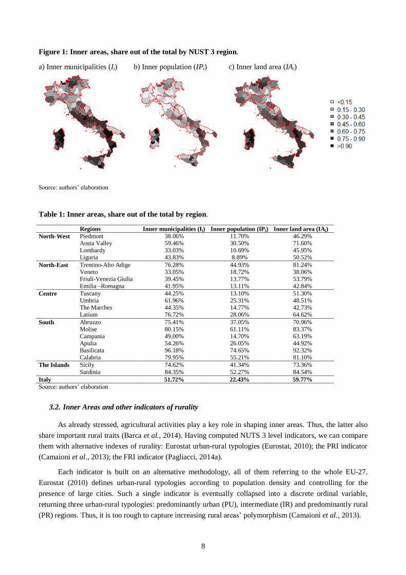
Figure 1 returns the values of each indicator at NUTS 3 level: Figure 1a maps Ii, Figure 1b maps IPi,

Figure 1c maps IAi. Both Figure 1a and Figure 1c return similar patterns; when focusing on population, the

share of inner areas at provincial level is generally lower. Just in a few Southern provinces, the share of

population living in inner municipalities is above 50%, while Northern NUTS 3 regions share a lower share

of inner areas than Southern ones. Exceptions are found across mountains areas.

Such a sharp North-South divide also emerges when looking at average values at regional level (Table

1). Among Italian regions, Liguria, Piedmont and Lombardy share the lowest shares of population living in

inner municipalities (less than 12%). On the opposite side, in three Southern regions (i.e., Basilicata, Molise

and Calabria) more than 55% of their population lives in inner areas. Thus, such a North-South divide should

be always taken into account in the rest of the analysis.

8

Figure 1: Inner areas, share out of the total by NUST 3 region.

a) Inner municipalities (Ii) b) Inner population (IPi) c) Inner land area (IAi)

Source: authors‟ elaboration

Table 1: Inner areas, share out of the total by region.

Regions Inner municipalities (Ii) Inner population (IPi) Inner land area (IAi)

North-West Piedmont 38.06% 11.70% 46.29% Aosta Valley 59.46% 30.50% 71.60% Lombardy 33.03% 10.69% 45.95% Liguria 43.83% 8.89% 50.52%

North-East Trentino-Alto Adige 76.28% 44.93% 81.24% Veneto 33.05% 18.72% 38.06% Friuli-Venezia Giulia 39.45% 13.77% 53.79% Emilia –Romagna 41.95% 13.11% 42.84%

Centre Tuscany 44.25% 13.10% 51.30% Umbria 61.96% 25.31% 48.51% The Marches 44.35% 14.77% 42.73% Latium 76.72% 28.06% 64.62%

South Abruzzo 75.41% 37.05% 70.96% Molise 80.15% 61.11% 83.37% Campania 49.00% 14.70% 63.19% Apulia 54.26% 26.05% 44.92% Basilicata 96.18% 74.65% 92.32% Calabria 79.95% 55.21% 81.10%

The Islands Sicily 74.62% 41.34% 73.36%

Sardinia 84.35% 52.27% 84.54%

Italy

51.72% 22.43% 59.77%

Source: authors‟ elaboration

3.2. Inner Areas and other indicators of rurality

As already stressed, agricultural activities play a key role in shaping inner areas. Thus, the latter also

share important rural traits (Barca et al., 2014). Having computed NUTS 3 level indicators, we can compare

them with alternative indexes of rurality: Eurostat urban-rural typologies (Eurostat, 2010); the PRI indicator

(Camaioni et al., 2013); the FRI indicator (Pagliacci, 2014a).

Each indicator is built on an alternative methodology, all of them referring to the whole EU-27.

Eurostat (2010) defines urban-rural typologies according to population density and controlling for the

presence of large cities. Such a single indicator is eventually collapsed into a discrete ordinal variable,

returning three urban-rural typologies: predominantly urban (PU), intermediate (IR) and predominantly rural

(PR) regions. Thus, it is too rough to capture increasing rural areas‟ polymorphism (Camaioni et al., 2013).

9

The PRI (PeripheRurality Indicator) is computed by Camaioni et al. (2013). Following a

multidimensional approach, they apply a conventional principal component analysis to a 24-variable dataset

(covering socio-demographic features, economic structure, land use, remoteness). Then, an ideal urban

benchmark (i.e., a region being extremely urban in Europe) is identified and statistical distances between any

other EU region and this benchmark are computed (Camaioni et al., 2013). So, for each region, the PRI

returns jointly the extent of rurality and peripherality.

Eventually, the FRI (Fuzzy Rurality Indicator) largely stresses the concept of urban-rural continuum.

It applies fuzzy logic to six input variables (covering role of agriculture, population density and

landscape/use of land) and it returns a final output (i.e., the FRI) and two intermediate outputs (Role of

Agriculture and Natural Landscape). Indicators range from 0 to 1, where 0 stands for completely urban; 1

stands for completely rural (Pagliacci, 2014a).

The statistical relationship between indicators of inner areas and indicators of rurality can be assessed

by means of Pearson correlation coefficients. Table 2 returns the correlation between Ii, IPi, IAi respectively

and the aforementioned three indicators of rurality computed for Italian NUTS 3 regions6. In any

specification, correlations are positive and statistically significant. Coefficients are larger for the FRI than for

the PRI, although the latter also assesses NUTS 3 regions remoteness (thus, a concept pretty similar to the

one referring to inner areas). Similar findings emerge when looking at the presence of inner municipalities

among different Eurostat urban-rural typologies. Point-biserial correlation between each dummy variable and

the presence of inner areas is consistent with expectations: indeed, correlation is positive for PR regions

(inner areas‟ share is larger in PR regions than in non-PR ones), and it is negative for both PU and IR ones.

When comparing average shares of inner areas among three typologies, similar evidence is returned: One-

Way ANOVA (Analysis of Variance) tests whether average values are statistically different or not.

Preliminarily, Levene‟s Test is computed to test whether groups‟ variances are equal.7 These tests show

statistically significant differences in any specification.

Thus, looking at these findings, a clear relationship between rural and inner areas emerges: despite

alternative definitions, those NUTS 3 regions showing larger shares of inner areas are also more rural than

other Italian areas. Thus, we can say National Strategy for Inner Areas implicitly refers to rural areas, as

well.

6 Here, just 107 observations are considered, as neither PRI nor FRI values are available for Monza and Brianza, Fermo, Barletta-Andria-Trani. Actually, those provinces were just instituted in 2004. 7 It tests the null hypothesis that groups‟ variances are equal. If they are, simple F test for the equality of means in a One-Way

ANOVA is performed; otherwise, Welch (1951) method is adopted.

10

Table 2: Relationships between the three inner indicators and indicators of rurality (PRI, FRI, Urban-

rural typology) (p-values in parenthesis).

Ii IPi IAi

Pearson correlation coefficients:

PRI (Camaioni et al., 2013) 0.522* 0.560* 0.487*

(0.000) (0.000) (0.000)

FRI (Pagliacci, 2014a) 0.657* 0.601* 0.638*

(0.000) (0.000) (0.000)

Point-biserial correlation:

Urban-rural typology:

PR regions 0.471* 0.538* 0.421*

(0.000) (0.000) (0.000)

IR regions -0.242* -0.269* -0.248*

(0.012) (0.005) (0.010)

PU regions -0.291* -0.341* -0.218*

(0.002) (0.000) (0.024)

Avg. comparison:

Avg. PR regions 0.689 0.461 0.677

Avg. IR regions 0.459 0.224 0.478

Avg. PU regions 0.343 0.112 0.407

Levene‟s test 0.182 6.608* 0.318

(0.834) (0.002) (0.728)

One-way ANOVA 17.919* 31.324* 12.871*

(0.000) (0.000) (0.000)

* Statistically significant at the 5% level

Source: authors‟ elaboration

4. QOL: DEFINING A MULTIDIMENSIONAL CONCEPT

4.1. Applying the Mazziotta-Pareto Index

QoL represents a multidimensional concept (MEA, 2005), including both economic aspects and

social-relational ones (Cagliero et al., 2011; Costanza et al., 2008; Petrosillo et al., 2013). Thus, measuring

QoL may be even harder than measuring the presence of inner areas: it requires the construction of a

composite and multidimensional index, which represents a challenging effort, for both scholars and policy

makers (OECD, 2008; Mazziotta and Pareto, 2014).

When specifically focusing on QoL as a multidimensional phenomenon, both „objective‟ and

„subjective‟ aspects play a role. The former dimension refers to physical and health status, personal income,

local standards of living and any other information gathered by national and regional institutions on a routine

basis (Malkina-Pykh and Pykh, 2008; Petrosillo et al., 2013). The latter one focuses on individuals‟

subjective experience of their lives (Land, 1996) as well as psychological responses (e.g., life and job

satisfaction and personal happiness). Assessing them is rather difficult: indicators referring to individual‟s

perceptions have to be obtained just by means of sociologic surveys and investigations (Shin and Johnson,

1978). Thus, although the European Foundation for the Improvement of Living and Working Conditions

follows a subjective approach in carrying out surveys on the level of quality of life across Europe (e.g.,

Eurofound, 2014), here we decided not to include any subjective measures of QoL, as they are not available

at NUTS 3 level. Rather, this analysis relies on objective indicators of QoL.

When focusing on this perspective, a wide literature has discussed the theoretical debate about the

main drivers of QoL at sub-national level. In particular, urban-rural divides have been widely investigated

(see for instance Cagliero et al., 2011; Florida et al., 2013; Shucksmith et al., 2009; Sørensen, 2014).

11

Nevertheless, the most cited QoL indicator, available in Italy at NUTS 3 level, is the one provided by the

financial newspaper “Il Sole 24 Ore”. Every year, it returns a QoL indicator based on 36 single variables,

grouped into six different thematic areas (economic wealth, business activities and employment, services and

environment, population, crime, leisure). Despite its popularity, this indicator suffers from some drawbacks.

Firstly, it assumes perfect substitutability among original variables (i.e., a good performance in a thematic

area may compensate a bad performance in another one). Secondly, different standard deviations among

each variable affect the final outcome8 (Mazziotta and Pareto, 2010a; 2010b; 2016). Lastly, the set of original

variables changes every year: this makes impossible to assess time comparisons.

To avoid aforementioned drawbacks, an alternative indicator is adopted here. In particular, the

Mazziotta-Pareto Index (MPI) is well consolidated in assessing QoL at local level. The MPI is a non-linear

composite index, which transforms individual variables into a standardized indicator. It sums original data

up, using arithmetic mean but adjusting it by a „penalty‟ coefficient, which is related to the variability

observed for each unit (Mazziotta and Pareto, 2016). Accordingly, those observations showing unbalanced

values of the initial variables are penalised, according to a non-compensatory perspective (Mazziotta and

Pareto, 2010a; 2016). In particular, here we adopt the following methodology to compute a QoL MPI.

Firstly, original variables standardisation occurs. Let‟s consider the original matrix X, whose generic element

is xij. It has n rows (observations) and m columns (variables), which are grouped into p thematic areas. From

X, a standardised matrix Z is computed (Mazziotta and Pareto, 2010a), whose generic element zij is

alternatively defined as follows:

10100

j

j

x

xij

ijS

Mxz

(4)

10100

j

j

x

xij

ijS

Mxz

(5)

Where: n

x

M

n

i

ij

x j

1 and

n

Mx

Sjx

n

i

ij

x j

2

1

)(

In particular, we apply equation (4) to those indicators that are concordant in sign with the QoL MPI;

otherwise, equation (5) is applied. Accordingly, p sub-indicators of QoL are computed, each of them

referring to a thematic area. Given h thematic areas, each of them comprising k variables, the h-th sub-

indicator of QoL is given by:

k

z

z

k

jjhki

ih

1

)1(,

(6)

The p sub-indicators ( ihz ) are then grouped together and a QoL MPI is returned as:

iii zzzi cvSMMPI (7)

Where:

p

z

M

p

h

ih

z i

1

,

p

Mz

Si

j

z

p

h

ih

z

2

1

)(

,

i

i

i

z

z

z M

Scv

The ii zz

cvS product represents the most innovative aspect of this approach, aimed at penalising those

units showing unbalanced values of the p thematic sub-indicators (Mazziotta and Pareto, 2016). In addition,

8 This distortion comes from the fact that the synthetic indicator is always computed through distances from a benchmark (i.e. the

best performing NUTS 3 region).

12

due to the standardisation provided by (4) or (5), each indicator‟s mean is 100 and each standard deviation is

10 (Mazziotta and Pareto 2010; Aiello and Attanasio, 2004).

Here, this methodology is applied to a set of 28 original variables, retrieved for each of 110 Italian

NUTS 3 regions. They refer to seven different thematic areas linked to QoL:

Wealth & economic competitiveness (3 indicators),

Services (3 indicators),

Labour market (5 indicators),

Neighbourhood safety (3 indicators),

Population (7 indicators),

Leisure (2 indicators),

Environment & Energy (5 indicators).

Thematic areas partially overlap with those provided by „Il Sole 24 Ore‟. Nevertheless, original

variables are open data published by the Open Coesione (OC) dataset: thus, we assure full comparability of

results across time. Table 3 clearly specifies the source of data, which in most cases is Istat, and reference

years: with the only exception of a few indicators, all data refer to years 2010 – 2014.

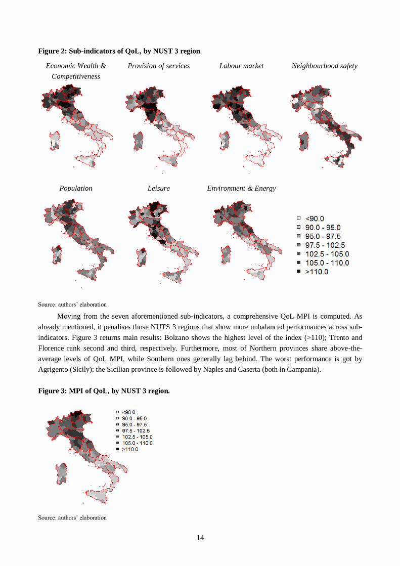
4.2. QoL and its sub-indicators: main territorial patterns

According to the aforementioned set of variables, seven different sub-indicators of QoL are returned.

Each sub-indicator shows standardised values. Figure 2 shows the values of each sub-indicator across Italian

provinces. Wealth and economic competitiveness show a strong North-South divide, confirming larger QoL

in the North of the country. Throughout Southern regions and the Islands, just Ragusa and Cagliari show

local values which are close to the national average. The provision of services is at a maximum in the

provinces of Emilia-Romagna and Tuscany, due to a long-lasting attention to these political items (Bripi et

al., 2011; Giordano and Tommasino, 2011). On the opposite side, education and health services are

particularly poor across Southern Regions (e.g., Molise, Basilicata and Calabria), but even in some provinces

close to Rome. As expected, labour market performance is poor in Southern provinces. On the opposite side,

the best performances occur throughout the provinces of the so-called Third Italy (Bagnasco, 1977; 1988),

namely in the North-East and alongside the Adriatic. Neighbourhood safety shows a less sharp North-South

divide: in fact, best performances are observed across mountain provinces (across both the Alps and the

Apennines). On the opposite side, metropolitan and urban provinces show poorer performances than rural

areas. Population sub-indicator shows a good performance across Emilia-Romagna and Trentino-Alto Adige.

Nevertheless, even in this case, Southern regions seem not lagging behind Northern ones, despite a lower

presence of foreign people. Leisure activities show a scattered pattern across Italy. Nonetheless, urban areas

and many Northern and Central Italian regions perform above the Italian average. Lastly, when focusing on

environment and energy, local performance is good across North-East NUTS 3 regions as well as in the

Aosta Valley. In the South, Sicily and Calabria show bad performances, whereas other inner NUTS 3

perform generally better.

13

Table 3: List of input variables, by thematic area.

Variable Definition

Effect

on

QoL

Year Source

Economic wealth & Competitiveness

Per capita GVA (€) Gross Value Added (current prices) per inhabitants, all sectors + 2013 Istat Per capita Export (€) Exports per inhabitants + 2014 Istat (OC)

Per capita Patents Patents registered to the European Patent Office, per million inhabitants + 2011 Istat on Eurostat

data (OC)

Provision of services

Diffusion of pre-school services

% of municipalities out of the total adopting pre-school services (e.g. nursery schools)

+ 2012

Istat (OC) Children 0-3 attending day care and pre-school

% of young children (aged 0-3 years) who use day care facilities and other pre-school services

+ 2012

Health emigration ratio Share of the out-migration in hospital in other regions out of total

hospital admissions - 2013

Labour market

Employment rate Employed persons (aged 15-64) over the number of people 15-64 (%) + 2014

Istat (OC)

Elderly people employment rate

Employed persons (aged 55-64) over the number of people 55-64 (%) + 2014

Youth unemployment rate

Unemployed persons (aged 15-24) over the number of persons 15-24 in the labour force (%)

- 2014

Unemployment rate Unemployed persons (aged 15+) over the number of persons (aged

15+) in the labour force (%) - 2014

Gender differences Differences in % points between male and female employment rates - 2014

Neighbourhood safety

Istat on Ministero Interno,

Dipartimento Pubblica

Sicurezza data (OC)

Rate of thefts Number of recorded thefts per a thousand inhabitants - 2013

Rate of robberies Number of recorded robberies per a thousand inhabitants - 2013

Rate of homicides Number of recorded intentional homicides per 100 thousand

inhabitants - 2013

Population

Population Density Inhabitants per km2 - 2014

Istat

Old-Age dependency ratio

Ratio of older dependents (people aged 65+) to the working-age population (15-64)

- 2014

Ageing Index Number of persons aged 65+ per hundred persons under age 15 - 2014 Internal net migration rate

Difference of immigrants and emigrants within the country in a year, divided per 1000 inhabitants

+ 2014

External net migration rate

Difference of immigrants and emigrants (from/to abroad) in a year, divided per 1000 inhabitants

+ 2014

Life expectancy at birth, males

Number of years a new-born male infant would live (assuming no changes in patterns of mortality throughout its life)

+ 2014

Life expectancy at birth, females

Number of years a new-born female infant would (assuming no changes in patterns of mortality throughout its life)

+ 2014

Leisure

Live theatre and live music performances

Tickets sold to live theatre and live music performances, per 100 inhabitants

+ 2007 Istat on SIAE

data (OC)

Tourists Number of overnight stays spent by national and foreign tourists in

tourist accommodations, per inhabitant + 2013 Istat (OC)

Environment and energy

Water use efficiency % of water distributed to customers out of the total volume introduced

into the municipality water network + 2008 Istat (OC)

Waste recycling Share of municipal waste recycled out of total solid waste (%) + 2014 Istat on ISPRA data (OC) Renewable energy % of GWh renewable energy to total energy production in GWh + 2010

Air quality monitoring network

Number of control stations of the air quality monitoring network, per 100 thousands inhabitants

+ 2012 Istat - Open Coesione

Discontinuity of electricity supply

Number of long-lasting interruptions in electricity supply (average number per single customer)

- 2014

Istat on Autorità Energia

elettrica, Gas, Sistema idrico

data (OC)

Source: author‟s elaboration

14

Figure 2: Sub-indicators of QoL, by NUST 3 region.

Economic Wealth &

Competitiveness

Provision of services Labour market Neighbourhood safety

Population Leisure Environment & Energy

Source: authors‟ elaboration

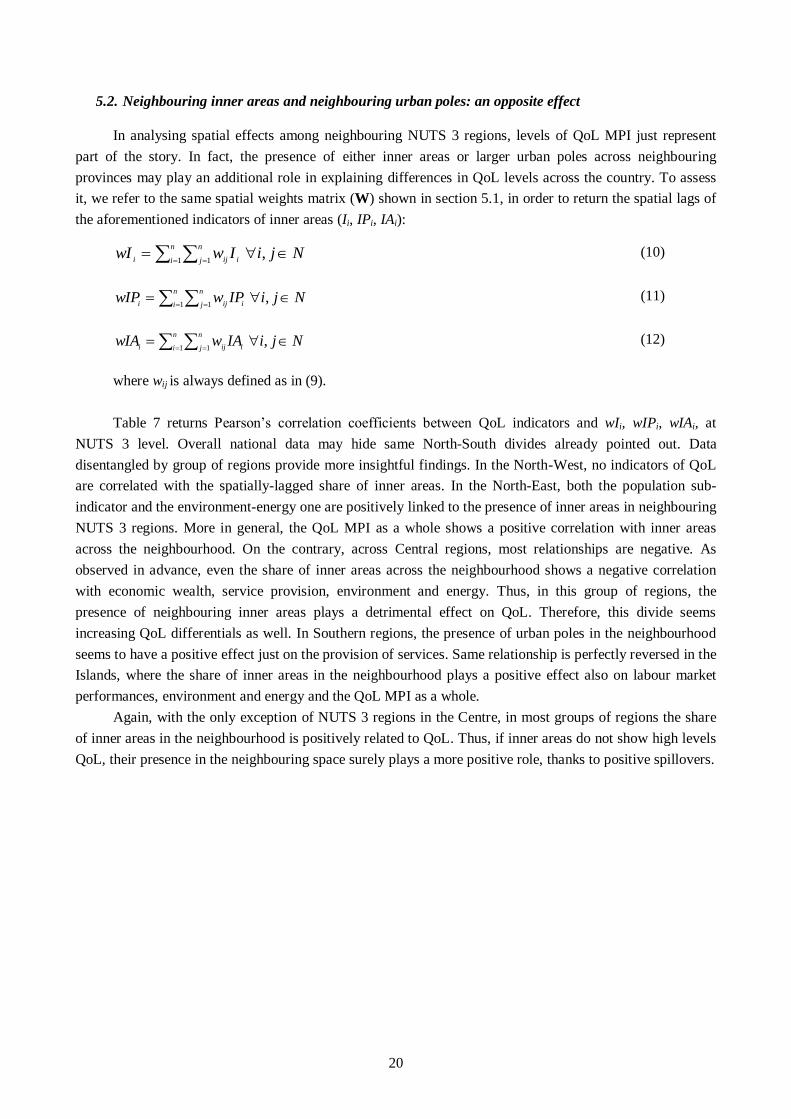
Moving from the seven aforementioned sub-indicators, a comprehensive QoL MPI is computed. As

already mentioned, it penalises those NUTS 3 regions that show more unbalanced performances across sub-

indicators. Figure 3 returns main results: Bolzano shows the highest level of the index (>110); Trento and

Florence rank second and third, respectively. Furthermore, most of Northern provinces share above-the-

average levels of QoL MPI, while Southern ones generally lag behind. The worst performance is got by

Agrigento (Sicily): the Sicilian province is followed by Naples and Caserta (both in Campania).

Figure 3: MPI of QoL, by NUST 3 region.

Source: authors‟ elaboration

15

Nevertheless, returning a ranking of provinces (which may change over time) is not the ultimate goal

of this work. Rather, in the following sections, we aim to analyse existing correlations between the presence

of inner areas and QoL.

4.3. QoL and inner areas: main relationships

Preliminarily, the analysis of Pearson correlation coefficients makes possible the assessment of the

main relationship between QoL levels and the presence of inner areas at NUTS 3 level (Table 4). Data at

national level seem to be clear: with the only exception of neighbourhood safety, which shows a positive

relation with the presence of inner areas, all other QoL dimensions are negatively correlated to the presence

of inner areas: thus, the larger the presence of inner areas at NUTS 3 level, the lower the level of QoL. These

results seem suggesting Italian inner areas generally suffer from low levels of QoL: thus, the launch of a

national strategy targeted to them is definitely good news. Furthermore, as shown in Section 3, given the

aforementioned relationship between the presence of both inner and rural areas, same results are expected to

hold even with respect to the rural part of the country.

Table 4: Pearson correlation coefficients between inner areas indicators and indicators of QoL (p-

values in parenthesis).

Ii IPi IAi

Economic Wealth & Competitiveness -0.504* -0.534* -0.443*

(0.000) (0.000) (0.000)

Provision of services -0.523* -0.518* -0.478*

(0.000) (0.000) (0.000)

Labour Market -0.405* -0.465* -0.352*

(0.000) (0.000) (0.000)

Neighbourhood safety 0.310* 0.350* 0.314*

(0.001) (0.000) (0.001)

Population -0.112 -0.200* -0.071

(0.245) (0.036) (0.459)

Leisure -0.213* -0.298* -0.193*

(0.025) (0.002) (0.043)

Environment & Energy -0.370* -0.388* -0.294*

(0.000) (0.000) (0.002)

QoL MPI -0.420* -0.470* -0.357* (0.000) (0.000) (0.000)

* Statistically significant at the 5% level

Source: authors‟ elaboration

Nevertheless, same data may hide some more complex patterns. In particular, two issues arise: i) non-

linearity in the relationship and ii) different patterns at sub-national level.

To appreciate non-linearity, let‟s just focus on the synthetic QoL MPI. Figure 4 returns the scattered

plots that link together the QoL MPI and the share of inner areas, according to both population and total area

at NUTS 3 level. Different patterns emerge. When considering the share of population living in inner areas

(IPi,), the negative relationship with QoL is mostly confirmed. Nevertheless, when taking into account total

areas (IAi), best performing NUTS 3 regions are those combining both urban poles and more inner areas

(namely those provinces showing intermediate levels of the IAi indicator). Actually, an inverted “U-shaped”

relationship seems occuring9. Thus, in Italy, both inner NUTS 3 regions and very urban ones tend to show

lower levels of QoL.

9 In each case, introducing a non-linear relation (i.e., y = x2+x) rather than a linear one improves estimates in terms of R2 values.

16

Figure 4: Non-linearity in the relationship between inner areas indicators (IPi and IAi) and QoL MPI.

Source: authors‟ elaboration

Nonetheless, non-linearity is just part of the story. A second issue to be taken into account refers to the

differences in the patterns observed at sub-national level. Indeed, in Section 3 we have just pointed out the

fact that on average Southern Italian regions show a larger presence of inner areas than Northern ones. Thus,

this sharp North-South divide could affect overall results in terms of QoL MPI. Accordingly, it could be

useful to disentangle previous results by macro-groups of regions. For sake of simplicity, here we refer to the

classification provided in Table 1 (North-West, North-East, Centre, South, the Islands): Table 5 shows

Person correlation coefficients per sub-indicator and per group of regions.

When disentangling by group of regions, most of differences between urban poles and inner areas

seem disappearing. In particular, the negative relationship between inner areas and QoL does no longer hold.

In fact, just a few sub-indicators appear to be statistically related to QoL:

North-West: a positive relation between the sub-indicator Neighbourhood safety and the presence of

inner areas occurs. Actually, the presence of large and unsafe metropolitan areas plays a role.

North-East: service provision is negatively tied to the presence of inner areas at NUTS 3 level, when

considering total population. Nevertheless, both „population‟ and „environment and energy‟ are

positively related to the presence of inner areas, as well as the QoL MPI.

Centre: a negative relation between QoL and the presence of inner areas affects many sub-indicators

of QoL (e.g. economic wealth, service provision, labour market, environment and energy). The only

sub-indicator that is positively related to the presence of inner areas is neighbourhood safety.

South: a negative relationship emerges when considering service provision and inner areas; on the

contrary, safety is positively associated with a larger presence of inner areas.

The islands: at NUTS 3 level, relationships between QoL and presence of inner areas are never

significant.

Thus, these data simply confirm inner areas‟ polymorphism: when controlling per single macro-

region, strikingly different results emerge. In the North-East, inner areas do not lag behind urban poles when

referring to QoL MPI, whereas opposite findings occurs when focusing on Central NUTS 3 regions. Thus,

these findings seem supporting the choice made by the national strategy about the implementation of a place-

based policy in accordance with regional governments: such a strategy seems to be more appropriate when

dealing with specific problems, which may occur locally.

17

Table 5: Pearson correlation coefficients between inner areas indicators and indicators of QoL by

macro-regions (p-values in parenthesis).

Wealth &

Competitiveness Services

Labour

Market

Neighbourhood

Safety Population Leisure

Environment

& Energy QoL MPI

North-

West

Ii -0.388 -0.237 0.088 0.493* -0.186 -0.016 0.062 -0.018

(0.056) (0.254) (0.676) (0.012) (0.373) (0.938) (0.768) (0.930)

IPi -0.218 -0.114 0.177 0.551* -0.082 -0.098 0.274 0.170

(0.295) (0.588) (0.398) (0.004) (0.697) (0.640) (0.185) (0.418)

IAi -0.362 -0.145 0.04 0.464* -0.100 0.021 0.074 0.048

(0.075) (0.488) (0.850) (0.019) (0.633) (0.922) (0.726) (0.820)

North-

East

Ii 0.212 -0.363 0.267 0.083 0.491* 0.181 0.587* 0.430*

(0.344) (0.097) (0.230) (0.713) (0.020) (0.421) (0.004) (0.046)

IPi 0.017 -0.487* 0.115 0.407 0.317 0.148 0.428* 0.334

(0.941) (0.022) (0.609) (0.060) (0.151) (0.510) (0.047) (0.129)

IAi 0.175 -0.378 0.239 0.177 0.452* 0.156 0.597* 0.423*

(0.437) (0.083) (0.284) (0.432) (0.035) (0.489) (0.003) (0.050)

Centre

Ii -0.663* -0.630* -0.504* 0.295 -0.451* -0.193 -0.428* -0.623*

(0.001) (0.002) (0.017) (0.182) (0.035) (0.390) (0.047) (0.002)

IPi -0.697* -0.703* -0.538 0.496* -0.421 -0.376 -0.454* -0.672*

(0.000) (0.000) (0.010) (0.019) (0.051) (0.084) (0.034) (0.001)

IAi -0.549* -0.533* -0.421 0.279 -0.324 -0.294 -0.238 -0.531*

(0.008) (0.011) (0.051) (0.208) (0.142) (0.184) (0.287) (0.011)

South

Ii 0.082 -0.529* 0.306 0.642* 0.194 -0.251 0.083 0.177

(0.704) (0.008) (0.146) (0.001) (0.363) (0.236) (0.700) (0.408)

IPi -0.021 -0.584* 0.179 0.670* 0.071 -0.380 0.047 0.045

(0.923) (0.003) (0.402) (0.000) (0.740) (0.067) (0.826) (0.836)

IAi 0.070 -0.573* 0.358 0.682* 0.207 -0.331 0.158 0.199

(0.745) (0.003) (0.086) (0.000) (0.333) (0.114) (0.462) (0.352)

The

Islands

Ii 0.091 0.229 0.476 0.264 -0.068 0.12 0.034 0.333

(0.729) (0.376) (0.053) (0.306) (0.794) (0.646) (0.896) (0.192)

IPi -0.107 0.138 0.310 0.219 -0.120 -0.07 0.171 0.180

(0.684) (0.597) (0.225) (0.398) (0.646) (0.792) (0.513) (0.488)

IAi 0.222 0.221 0.421 0.080 -0.090 0.327 -0.059 0.279

(0.391) (0.394) (0.093) (0.759) (0.731) (0.200) (0.821) (0.279)

* Statistically significant at the 5% level

Source: authors‟ elaboration

5. THE ROLE OF THE NEIGHBOURING S

Italian provinces are characterised by a narrow extension: on average, the surface of an Italian

province is 2 745 km2, i.e. a square whose side is just 52 km. According to these figures, we cannot ignore

the fact that people live, work and spend part of their own leisure time across neighbouring provinces. Thus,

it could be misleading to focus any analysis on QoL at NUTS 3 level just on the relationships between it and

socio-economic features in the same NUTS 3 region. In fact, even the characteristics of neighbouring

provinces may affect QoL levels, having an impact on people‟s everyday life10. To this respect, two major

characteristics of neighbouring provinces should be taken into account: the extent of QoL and the presence

of either inner areas or urban poles. Let‟s consider two effects separately.

5.1. Spatial autocorrelation: QoL across neighbouring provinces

The simplest way to assess the QoL differentials across neighbouring observations is represented by

the analysis of global and local indicators of spatial autocorrelation. According to the first law of geography

(Tobler, 1970), specific statistical methodologies are implemented to highlight patterns of spatial association,

10 A similar idea was originally suggested and tested by Pagliacci (2014b), in a preliminary analysis on QoL patterns across urban

and rural Italian provinces. Nonetheless, that work simply considered the rough indicator returned by “Il Sole 24 Ore”.

18

by formally measuring the degree of dependency among observations within a given geographic space

(Anselin 1988; 1995). Firstly, global Moran‟s I statistics tests for the presence of spatial dependence.

Moran‟s I test is a synthetic measure of global spatial autocorrelation, which is computed as follows (Moran,

1950; Cliff and Ord, 1981):

Nji

yy

yyyyw

w

nI

n

i i

n

i

n

j jiij

n

i

n

j ij

,,

1

2

1 1

1 1

(8)

where yi and yj are observations of a given variable in locations i and j, and ijw is the generic element of a (n

x n) row-standardized spatial weights matrix (W) defined as follows:

n

j ij

ij

ij

w

ww

1

*

*

(9)

The generic element *

ijw in (9) can take two alternative values: 1* ijw if ji and )(iNj ;

0* ijw if )(iNjandjiorji , where N(i) is the set of neighbours of the i-th region. N(i), thus W,

can be identified in several alternative ways. Literature has emphasized the fact there is no univocal

preferable specification of W (Anselin, 1988). Despite alternative suitable weight matrices (e.g. those based

on the nearest neighbours), here W is a first-order queen contiguity matrix. Thus, two regions are considered

as neighbours only if they share a common boundary or vertex (Anselin, 1988). On average, each

observation shows 4.45 neighbouring regions11

.

This row-standardized spatial weights matrix (W) allows computing global Moran‟s I statistic (thus

their degree of spatial dependency) on both the QoL MPI and other sub-indicators of QoL. According to a

global approach, it returns the degree of overall linear association between a vector of observed values and

the spatially weighted averages of neighbouring observations. Thus, it does not allow the detection of

specific regional structures of spatial autocorrelation (i.e., either spatial cluster or spatial outliers): to do that,

local approaches in the analysis of spatial association may help. As a local indicator of spatial association,

here we adopt Local Indicator of Spatial Association – LISA (Anselin 1995; Anselin et al., 1996): it is

similar to the global Moran‟s I statistic, but it is region-specific. It tests the hypothesis of random distribution

by comparing values in specific locations and values in their neighbourhood (as defined by W). Local

Moran‟s statistics returns the distribution of local spatial clusters, which are groups of neighbouring locations

showing signicant LISA values. At a given significance level, such as 1%, it is possible to detect five

alternative cases (Anselin, 1995): i) Hot spots (locations with high values and similar neighbours); ii) Cold

spots (locations with low values and similar neighbours); iii) Spatial outliers (locations with high values but

with low-value neighbours); iv) Spatial outliers (locations with low values but with high-value neighbours);

v) Locations with no significant local autocorrelation.

Table 6 returns the values for both the global and the local Moran‟s I statistics, computed for both sub-

indicators of QoL and the QoL MPI itself. A positive spatial autocorrelation occurs for all indicators but

neighbourhood safety. The question thus becomes whether this general tendency to clustering yields to some

given spatial clusters or not. The analysis on the LISA values returns information about spatial clusters in

larger detail. Table 6 returns the number of NUTS 3 regions within each of the aforementioned five

typologies of regions (at a 1% level of significance). Results are straightforward. In all cases, no spatial

11 Most of Italian NUTS3 regions show either 4 or 5 neighbours. Nevertheless, the least connected province has just 1 neighbour,

whereas the most connected one has 9 neighbours.

19

outliers are detected (confirming the sharp tendency to a positive spatial autocorrelation of observed values).

In particular, neighbourhood safety and leisure are characterised by a fewer numbers of both hot and cold

spots, whereas economic wealth, service provision and environment are much more clustered in space.

Referring to the QoL MPI, 10 NUTS 3 regions are defined as hot spots, thus they benefit from large QoL

levels even across their neighbourhood. Conversely, in 20 cases, low QoL levels are reinforced by bad

performances even across neighbouring provinces.

Table 6: Global Moran’s I statistics (p-value in parenthesis) and Local Moran’s I statistics (number of

NUTS 3 regions within each typology).

Global Moran‟s I Local Moran‟s I (LISA)

Moran's I Hot spots (1) Cold spots (2)

Spatial outliers

(3 & 4)

No local

autocorrelation (5)

Wealth 0.678* 14 11 0 85 (0.000)

Services

0.763* 16 13 0 81 (0.000)

Labour Market

0.809* 6 23 0 81 (0.000)

Neighborhood

Safety

0.057 0 3 0 107

(0.152)

Population 0.289* 7 6 0 97 (0.000)

Leisure

0.215* 5 0 0 105 (0.000)

Environment

0.630* 7 14 0 89 (0.000)

MPI

0.802* 10 20 0 80 (0.000)

* Statistically significant at the 5% level

Source: authors‟ elaboration

For the sake of simplicity, Figure 5 just maps the spatial clusters occurring when considering the

comprehensive QoL MPI. It is easy to notice that hot spots are mostly located across North-Eastern Italy and

partially among Central regions, returning two separated group of provinces. Thus, the North-East emerges

as the best area of the country in terms of QoL levels. Conversely, cold spots cover most of Southern

regions, from Campania and Apulia to Calabria and Sicily. In particular, the presence of neighbouring NUTS

3 regions sharing similar QoL MPI low values may reinforce their lags compared to Northern Italy. It may

have a negative impact on dynamic performances as well.

Figure 5: Hot and cold spots – QoL MPI.

Source: authors‟ elaboration

20

5.2. Neighbouring inner areas and neighbouring urban poles: an opposite effect

In analysing spatial effects among neighbouring NUTS 3 regions, levels of QoL MPI just represent

part of the story. In fact, the presence of either inner areas or larger urban poles across neighbouring

provinces may play an additional role in explaining differences in QoL levels across the country. To assess

it, we refer to the same spatial weights matrix (W) shown in section 5.1, in order to return the spatial lags of

the aforementioned indicators of inner areas (Ii, IPi, IAi):

NjiIwwIn

i

n

j iiji

,1 1

(10)

NjiIPwwIPn

i

n

j iiji

,1 1

(11)

NjiIAwwIAn

i

n

j iiji

,1 1

(12)

where wij is always defined as in (9).

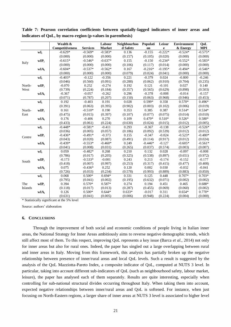
Table 7 returns Pearson‟s correlation coefficients between QoL indicators and wIi, wIPi, wIAi, at

NUTS 3 level. Overall national data may hide same North-South divides already pointed out. Data

disentangled by group of regions provide more insightful findings. In the North-West, no indicators of QoL

are correlated with the spatially-lagged share of inner areas. In the North-East, both the population sub-

indicator and the environment-energy one are positively linked to the presence of inner areas in neighbouring

NUTS 3 regions. More in general, the QoL MPI as a whole shows a positive correlation with inner areas

across the neighbourhood. On the contrary, across Central regions, most relationships are negative. As

observed in advance, even the share of inner areas across the neighbourhood shows a negative correlation

with economic wealth, service provision, environment and energy. Thus, in this group of regions, the

presence of neighbouring inner areas plays a detrimental effect on QoL. Therefore, this divide seems

increasing QoL differentials as well. In Southern regions, the presence of urban poles in the neighbourhood

seems to have a positive effect just on the provision of services. Same relationship is perfectly reversed in the

Islands, where the share of inner areas in the neighbourhood plays a positive effect also on labour market

performances, environment and energy and the QoL MPI as a whole.

Again, with the only exception of NUTS 3 regions in the Centre, in most groups of regions the share

of inner areas in the neighbourhood is positively related to QoL. Thus, if inner areas do not show high levels

QoL, their presence in the neighbouring space surely plays a more positive role, thanks to positive spillovers.

21

Table 7: Pearson correlation coefficients between spatially-lagged indicators of inner areas and

indicators of QoL, by macro-region (p-values in parenthesis)

Wealth &

Competitiveness Services

Labour

Market

Neighbourhoo

d Safety

Populati

on

Leisur

e

Environment

& Energy

QoL

MPI

Italy

wIi -0.629* -0.569* -0.583* 0.136 -0.155 -0.222* -0.524* -0.575*

(0.000) (0.000) (0.000) (0.157) (0.105) (0.020) (0.000) (0.000)

wIPi -0.615* -0.546* -0.637* 0.155 -0.150 -0.234* -0.552* -0.583*

(0.000) (0.000) (0.000) (0.106) (0.117) (0.014) (0.000) (0.000)

wIAi -0.604* -0.537* -0.562* 0.167 -0.216* -0.195* -0.494* -0.546*

(0.000) (0.000) (0.000) (0.079) (0.024) (0.041) (0.000) (0.000)

North-West

wIi -0.403* -0.122 -0.356 0.221 -0.379 0.024 -0.800 -0.246

(0.046) (0.560) (0.091) (0.288) (0.062) (0.910) (0.704) (0.235)

wIPi -0.070 0.252 -0.274 0.192 0.121 -0.101 0.027 0.140

(0.739) (0.224) (0.184) (0.357) (0.565) (0.629) (0.898) (0.503)

wIAi -0.367 -0.057 -0.262 0.296 -0.378 -0.008 -0.014 -0.157

(0.071) (0.787) (0.207) (0.150) (0.063) (0.968) (0.946) (0.453)

North-East

wIi 0.192 -0.403 0.191 0.028 0.599* 0.358 0.570* 0.496*

(0.391) (0.063) (0.395) (0.902) (0.003) (0.102) (0.006) (0.019)

wIPi 0.161 -0.510* 0.190 0.353 0.385 0.387 0.514* 0.534*

(0.475) (0.015) (0.397) (0.107) (0.077) (0.075) (0.014) (0.010)

wIAi 0.176 -0.406 0.270 0.109 0.479* 0.510* 0.526* 0.580*

(0.433) (0.061) (0.224) (0.630) (0.024) (0.015) (0.012) (0.005)

Centre

wIi -0.448* -0.581* -0.411 0.293 -0.367 -0.138 -0.524* -0.526*

(0.036) (0.005) (0.057) (0.186) (0.092) (0.539) (0.012) (0.012)

wIPi -0.436* -0.491* -0.373 0.155 -0.347 -0.024 -0.523* -0.480*

(0.043) (0.020) (0.087) (0.491) (0.114) (0.917) (0.012) (0.024)

wIAi -0.439* -0.553* -0.460* 0.249 -0.446* -0.127 -0.605* -0.561*

(0.041) (0.008) (0.031) (0.265) (0.037) (0.574) (0.003) (0.007)

South

wIi 0.059 -0.482* 0.268 0.210 0.132 0.028 -0.097 -0.008

(0.786) (0.017) (0.205) (0.325) (0.538) (0.897) (0.651) (0.972)

wIPi -0.173 -0.533* -0.001 0.243 0.213 -0.174 -0.152 -0.177

(0.418) (0.007) (0.997) (0.253) (0.317) (0.415) (0.477) (0.408)

wIAi 0.075 -0.436* 0.252 0.120 0.002 0.030 -0.032 -0.041

(0.726) (0.033) (0.234) (0.578) (0.993) (0.889) (0.883) (0.850)

The Islands

wIi 0.068 0.500* 0.694* 0.331 0.125 0.448 0.707* 0.703*

(0.795) (0.041) (0.002) (0.195) (0.632) (0.071) (0.002) (0.002)

wIPi 0.394 0.570* 0.587* 0.274 0.194 0.451 0.465 0.688*

(0.118) (0.017) (0.013) (0.287) (0.455) (0.069) (0.060) (0.002)

wIAi 0.126 0.500* 0.644* 0.633* -0.017 0.311 0.654* 0.770*

(0.631) (0.041) (0.005) (0.006) (0.948) (0.224) (0.004) (0.000)

* Statistically significant at the 5% level

Source: authors‟ elaboration

6. CONCLUSIONS

Through the improvement of both social and economic conditions of people living in Italian inner

areas, the National Strategy for Inner Areas ambitiously aims to reverse negative demographic trends, which

still affect most of them. To this respect, improving QoL represents a key issue (Barca et al., 2014) not only

for inner areas but also for rural ones. Indeed, the paper has singled out a large overlapping between rural

and inner areas in Italy. Moving from this framework, this analysis has partially broken up the negative

relationship between presence of inner/rural areas and local QoL levels. Such a result is suggested by the

analysis of the QoL Mazziotta-Pareto Index, a composite indicator of QoL, computed at NUTS 3 level. In

particular, taking into account different sub-indicators of QoL (such as neighbourhood safety, labour market,

leisure), the paper has analysed each of them separately. Results are quite interesting, especially when

controlling for sub-national structural divides occurring throughout Italy. When taking them into account,

expected negative relationships between inner/rural areas and QoL is softened. For instance, when just

focusing on North-Eastern regions, a larger share of inner areas at NUTS 3 level is associated to higher level

22

of QoL. Furthermore, even neighbourhood safety (a key driver of QoL) is generally larger in more

inner/rural NUTS 3 regions than in urban ones.

If it is hard to find conclusive results about the relationship between inner areas and QoL (which in

most cases is not linear, as well), spatial aspects make the picture even more complex. People may spend part

of their lives out of their own province, thus even neighbourhood space is expected to matter when dealing

with QoL. Here, main results strongly support this idea. Both QoL sub-indicators and QoL MPI show a

positive spatial autocorrelation. Furthermore, it is possible to detect groups of regions whose neighbours

share similar QoL levels. It follows that even the local development may be influenced by neighbouring

regions‟ development, showing a kind of spatially locked-in paths. Thus, spatial spillovers are expected to

affect place-based policies, which may be more or less effective, according to each region‟s neighbouring

space. The same holds true when considering the presence of inner areas among neighbouring regions: for

instance, this work proves that being located close to a province with a higher share of inner areas could have

positive effects on QoL, especially in the North-East and in the South.

Thus, this analysis returns a clear picture about inner areas‟ polymorphism. Indeed, some of them

show much socio-economic potential, even with respect to some specific sub-indicators of QoL, while others

still lag behind. In particular, the „innermost‟ areas in the South are the weakest ones, throughout Italy. Such

a finding has important policy implications, even with respect to the National Strategy for Inner Areas. The

top-down decision, carried out by the Italian central government, to focus on inner areas‟ development has

been relevant. Nevertheless, it is important to maintain the decision-making process partially decentralised,

in order to identify the most appropriate policy tools to be implemented and the neediest areas to be targeted.

Besides these considerations, this paper points out the effectiveness of the innovative approach chosen

by the National Strategy for Inner Areas, which highlights territorial unbalances in terms of people‟s needs

rather than territorial features. Indeed, just the provision of essential services to the population is seen as the

main engine for local development, now and in the future. Such an approach would allow both scholars and

policymakers to go beyond traditional urban-rural divides, which in fact are mostly considered by EU

policies (such as the Rural Development Policy). Although providing partially overlapping results, a focus

on inner areas seems stressing inter-sectoral policies as the best answer to overcome territorial divides and to

cope with population changes, both in Italy and in the EU.

REFERENCES

Aiello, P. and Attanasio, M. (2004) How to Transform a Batch of Single Indicators to Make Up a Unique

One? Atti della XLII riunione scientifica della Società Italiana di Statistica (Sessioni plenarie e

specializzate): 327-338.

Anselin, L. (1988), Spatial Econometrics: Methods and Models. Dordrecht: Kluwer Academic Publishers.

Anselin, L. (1995), Local Indicators of spatial association – LISA. Geographical Analysis, 27: 93-115.

Anselin, L., Bera, A.K., Florax, R.J.G.M., and Yoon, M.J. (1996), Simple diagnostic tests for spatial

dependence, Regional Science and Urban Economics, 26: 77-104.

Bagnasco, A. (1977), Tre Italie: la problematica territoriale dello sviluppo economico italiano. Bologna: Il

Mulino.

Bagnasco, A. (1988), La costruzione sociale del mercato. Bologna: Il Mulino.

Barca, F., McCann, P. and Rodríguez-Pose, A. (2012), The Case for Regional Development Intervention:

Place-Based versus Place-Neutral Approaches. Journal of Regional Science 52(1): 134-152.

23

Barca, F., Casavola, P. and Lucatelli, S. (eds.) (2014), A strategy for inner areas in Italy: definition,

objectives, tools and governance. Materiali Uval Series 31.

Bertolini, P., Montanari, M., Peragine, V. (2008) Poverty and Social Exclusion in Rural Areas. Bruxelles:

European Commission.

Bripi, F., Carmignano, A. and Giordano, R. (2011), La qualità dei servizi pubblici in Italia. Occasional

Paper 84. Roma: Bankitalia.

Cagliero, R., Cristiano, S., Pierangeli, F. and Tarangioli, S. (2011), Evaluating the Improvement of Quality

of Life in Rural Areas. Paper presented at 122nd EAAE Seminar. Ancona (Italy), 17-18 February.

Camaioni, B., Esposti, R., Lobianco, A., Pagliacci, F. and Sotte, F. (2013), How rural the EU RDP is? An

analysis through spatial funds allocation. Bio-based and Applied Economics 2(3): 277–300.

Christaller, W. (1933), Die zentralen Orten in Süddeutsch-Land. Jena: Gustav Fischer.

Cliff, A. and Ord, J.K. (1981), Spatial processes: Models and applications. London: Pion.

Copus, A., Melo, P.C., Kaup, S., Tagai, G. and Artelaris, P. (2015), Regional poverty mapping in Europe –

Challenges, advances, benefits and limitations. Local Economy. DOI: 10.1177/0269094215601958.

Costanza, R., Fisher, B., Ali, S., Beer, C., Bond, L., Boumans, R., Danigelis, N.L., Dickinson, J., Elliott, C.,

Farley, J., Elliott Gayer, D., MacDonald Glenn, L., Hudspeth, T.R., Mahoney, D.F., McCahill, L., McIntosh,

B., Reed, B., Turab Rizvi, A., Rizzo, D.M., Simpatico, T. and Snapp, R. (2008), An Integrative Approach to

Quality of Life Measurement, Research, and Policy. S.A.P.I.EN.S. 1(1). Online since 19.12.08.

http://sapiens.revues.org/169.

Dematteis, G.(1986), Urbanization and counter - urbanization in Italy, Ekistics, 53 (316/317): 26-33.

Dijkstra, L. and Poelman, H. (2008), Remote Rural Regions. How proximity to a city influences the

performance of rural regions, Regional Focus, 1.

Eurofound (2014), Quality of life in urban and rural Europe. Luxembourg: Publications Office of the

European Union.

Eurostat (2010), A revised urban-rural typology. In Eurostat, Eurostat regional yearbook 2010. Luxembourg:

Publications Office of the European Union: 240-253.

Florida, R., Mellander, C. and Rentfrow, P.J. (2013), The Happiness of Cities, Regional Studies 47(4): 613-

627.

Giordano, R. and Tomasino, P. (2011), Public sector efficiency and political culture, Working papers

Bankitalia, 786. Roma: Bankitalia.

Hoggart, K, Buller, H. and Black, R. (1995), Rural Europe; Identity and Change. London: Edward Arnold.

Land, K.C. (1996), Social indicators and the quality of life: where do we stand in the mid-1990s? SINET 45:

5-8.

Lucatelli, S., Carlucci, C. and Guerrizio M.A. (2013), A Strategy for the „Inner Areas‟ of Italy. Proceedings

of the 2nd

EURUFU (Education, Local Economy and Job Opportunities in Rural Areas) Scientific

Conference. Asti (Italy), 8 October.

Malkina-Pykh, I.G. and Pykh, Y.A. (2008). Quality-of-life indicators at different scales: theoretical

background, Ecological Indicators 8: 854-862.

Matthews, A. (2013), Greening Agricultural Payments in the EU‟s Common Agricultural Policy. Bio-based

and Applied Economics 2(1): 1-27.

Mazziotta, M. and Pareto, A. (2010a), La sintesi degli indicaotri di qualità della vita: un approccio non

compensativo. Paper presented at “Congresso Qualità della vita. Riflessioni, studi e ricerche in Italia”,

Firenze, Italia.

Mazziotta, M. and Pareto, A. (2010b), Measuring quality of life: an approach based on the non-

substitutability of indicators, Statistica e Applicazioni 8(2): 169-180.

24

Mazziotta, M. and Pareto, A. (2015). On a Generalized Non-compensatory Composite Index for Measuring

Socio-economic Phenomena. Social Indicators Research, DOI 10.1007/s11205-015-0998-2

Mazziotta, M. and Pareto, A. (2016), Methods for Constructing Non-compensatory Composite Indices: A

Comparative Study, Forum for Social Economics, 45(2-3): 213-229.

Millennium Ecosystem Assessment (MEA) (2005), Ecosystems and Human Wellbeing. Washington, DC:

Island Press.

Moran, P.A.P. (1950), Notes on continuous stochastic phenomena, Biometrika 37: 17–23.

OECD (2008), Handbook on Constructing Composite Indicators. Methodology and user guide. Paris: OECD

Publications

OECD (2009), OECD Rural Policy Reviews: Italy. Paris: OECD Publications.

Pagliacci, F. (2014a), Are EU Rural Areas still Lagging behind Urban Areas? An Analysis through Fuzzy

Logic. Paper presented at 3rd AIEAA Conference, “Feeding the Planet and Greening Agriculture: Challenges

and opportunities for the bio-economy”, 25-27 June, 2014, Alghero, Italy.

Pagliacci, F. (2014b), L‟erba del vicino è davvero più verde? Un‟analisi sulla qualità della vita nelle province

urbane e rurali, AgriRegioniEuropa, 10(39): 54-57.

Paniagua, A. (2012), The Rural as a Site of Recreation: Evidence and Contradictions in Spain from a

Geographical Perspective. Journal of Tourism and Cultural Change 10(3): 264-275.

Petrosillo, I., Costanza, R., Aretano, R., Zaccarelli, N. and Zurlini, G. (2013), The use of subjective

indicators to assess how natural and social capital support residents‟ quality of life in a small volcanic island,

Ecological Indicators 24:, 609-620.

Shin, D.C. and Johnson, D.M. (1978), Avowed happiness as an overall assessment of the quality of life,

Social Indicators Res. 5: 475-492.

Shucksmith, M., Cameron, S., Pichler, F. and Merridew, T. (2009), Urban-rural differences in Quality of

Life across the EU, Regional Studies 43(10): 1275-1289.

Sørensen, J.F. (2014), Rural–urban differences in life satisfaction: Evidence from the European Union.

Regional Studies 48(9): 1451-1466.

Tobler, W. R. (1970), A computer movie simulating urban growth in the Detroit region, Economic

Geography 46: 234–240.

Welch, B.L. (1951), On the comparison of several mean values: an alternative approach. Biometrika 38:

330–336.