J. Math. Biol. (2015) 71:1269–1298DOI 10.1007/s00285-015-0857-4 Mathematical Biology

Delay induced stability switch, multitype bistabilityand chaos in an intraguild predation model

Hongying Shu · Xi Hu · Lin Wang · James Watmough

Received: 12 June 2014 / Revised: 3 January 2015 / Published online: 6 February 2015© Springer-Verlag Berlin Heidelberg 2015

Abstract In many predator–prey models, delay has a destabilizing effect and inducesoscillations; while in many competitionmodels, delay does not induce oscillations. Byanalyzing a rather simple delayed intraguild predation model, which combines boththe predator–prey relation and competition, we show that delay in intraguild predationmodels promotes very complex dynamics. The delay can induce stability switchesexhibiting a destabilizing role as well as a stabilizing role. It is shown that three typesof bistability are possible: one stable equilibrium coexists with another stable equi-librium (node-node bistability); one stable equilibrium coexists with a stable periodicsolution (node-cycle bistability); one stable periodic solution coexists with anotherstable periodic solution (cycle-cycle bistability). Numerical simulations suggest thatdelay can also induce chaos in intraguild predation models.

Keywords Intraguild predation · Time delay · Bistability · Chaos · Stability switch

Mathematics Subject Classification 92B05 · 34D20 · 34K18

Research is partially supported by NSERC Discovery Grant and NSERC Strategic Project Grant(LW, JW).

H. ShuDepartment of Mathematics, Tongji University, Shanghai 200092, P. R. China

X. Hu · L. Wang · J. Watmough (B)Department ofMathematics andStatistics,University ofNewBrunswick, FrederictonE3B5A3,Canadae-mail: watmough@unb.ca

L. Wange-mail: lwang2@unb.ca

123

1270 H. Shu et al.

1 Introduction

There has been numerous biological evidence showing that intraguild predation (IGP)is a widespread interaction within many ecological communities (Arim and Marquet2004; Fedriani et al. 2000; Hall 2011; Hickerson et al. 2005; Lucas 2005; Pimmand Lawton 1978). IGP occurs when a predator and prey share a basal resource. Itsignificantly influences the distribution, abundance, persistence and evolution of manyspecies, and thus affects the structure of ecological communities (Drolet et al. 2009;Polis and Holt 1992; Polis et al. 1989). Since the pioneering work of Polis and others(Polis and Holt 1992; Polis et al. 1989), a growing number of biological papers on IGPhave been published, demonstrating the ubiquity and the importance of this interaction.

One of the very first general mathematical models describing IGP was developedby Holt and Polis (1997). Their model takes the following form:

R′(t) = b(R(t)) − f1(R(t), N (t), P(t))N (t) − f2(R(t), N (t), P(t))P(t),

N ′(t) = g1(R(t), N (t), P(t))N (t) − f3(R(t), N (t), P(t))P(t) − d1(N (t)),

P ′(t) = g2(R(t), N (t), P(t))P(t) + g3(R(t), N (t), P(t))P(t) − d2(P(t)),

(1)

where R(t), N (t) and P(t) are the densities of the basal resource, the intraguild (IG)prey, and the IG predator, respectively. The function b(R) describes the growth of Rin the absence of N and P , the functions fi , i = 1, 2, 3 are functional responses, andthe functions gi , i = 1, 2, 3 are numerical responses. The indices refer to the threepredator–prey interactions: 1 and 2, predation on the basel resource by the IG preyand predator, respectively, and 3, predation on the IG prey by the IG predator. Thefunctional responses model the rate of decline of the respective prey due to predation,and the numerical responses model the corresponding increase in respective predatordensities. The functions d1 and d2 are the death functions of the IG predator and prey,respectively.

Previous studies of IGP models have focused on special forms of the functionaland numerical responses: Abrams and Fung (2010) and Tanabe and Namba (2005)mainly provide numerical simulations; Velazquez et al. (2005) and Hsu et al. (2015)consider the case with a bilinear functional response for the three predation terms;Verdy and Amarasekare (2010), Freeze et al. (2014) and Hsu et al. (2013) considerHolling type II, ratio-dependent and Beddington–DeAngelis responses respectively;Kang and Wedekin (2013) consider two models, one is referred to as the IGP modelwith generalist predator and the other is referred to as the IGP model with specialistpredator, and bothmodels have bilinear functional responses for predation on the basalresource ( f1 and f2) and a Holling-Type III functional response for predation on theIG prey by the IG predator ( f3).

The aforementioned models only describe ideal populations and assume that thepredator population can instantaneously convert the consumption to its growth. In thedynamics of real populations, there are reaction-time lags in the response of predators(MacDonald 1978; Wangersky and Cunningham 1957), which appear as delays in thenumerical response functions. It has been shown that such time delays can destabilizean otherwise stable equilibrium and induce oscillations in predator–prey models (Fan

123

A Delayed IGP Model 1271

and Wolkowicz 2010; Li et al. 2014; Ruan 2009; Shi 2013; Song and Wei 2005; Xiaoand Ruan 2001) and food-chain models (Maiti et al. 2008). In contrast, similar delaysdo not cause sustained oscillations in competition models with monotone responsefunctions (Wolkowicz and Xia 1997). Note that the IGPmodels involve both predator–prey interactions and competition. Hence, it is of great interest to explore the role ofdelay in determining the dynamics of IGPmodels. Yamaguchi et al. (2007) have begunthis by considering an IGP model with stage structure of the IG predator. In this paper,we include a time delay in the IG prey’s numerical response and examine how sucha delay affects the number and types of alternative stable states in the IGP module.To characterize the impact of delay, we select the simplest functional and numericalresponses in Eq. (1) and consider the following system of delay-differential equations:

R′(t) = r R(t)

(1 − R(t)

K

)− c1R(t)N (t) − c2R(t)P(t),

N ′(t) = e1c1R(t − τ)N (t − τ) − c3N (t)P(t) − m1N (t),

P ′(t) = e2c2R(t)P(t) + ε3c3N (t)P(t) − m2P(t).

(2)

Here, logistic growth is assumed for the basal resource with carrying capacity K . Thepositive constants ci , i = 1, 2, 3, are the predation rates for the three predator–preyinteractions numbered as above. The positive constants ei are the conversion rates ofprey to predator for the three interactions, and the positive constants m1 and m2 arethe natural death rates of IG prey and IG predator, respectively.

Wewill show that the delay, τ , inModel (2) promotes very complex dynamics.Moreprecisely, we show that delay can induce stability switches. In addition, we show thatdelay can induce three distinct patterns of bistability and even chaos. The three typesof bistability include a node-node bistability, where one stable equilibrium coexistswith another stable equilibrium, a node-cycle bistability, where one stable equilibriumcoexists with a stable periodic solution, and a cycle-cycle bistability, where one stableperiodic solution coexists with another stable periodic solution.

Model (2) can be rescaled to simplify the analysis. We introduce the new variablesx = R/K , y = c1N/r, z = c2P/r , and define new parameters β1 = e1c1K/r, β2 =e2c2K/r, γ1 = m1/r, γ2 = m2/r, α = c3/c2 and β3 = e3c2/c1. In addition, werescale t and τ by r , but for simplicity, keep the same notation. With these rescalings,Model (2) becomes

x ′(t) = x(t) (1 − x(t)) − x(t)y(t) − x(t)z(t),

y′(t) = β1x(t − τ)y(t − τ) − γ1y(t) − αy(t)z(t),

z′(t) = β2x(t)z(t) − γ2z(t) + β3αy(t)z(t).

(3)

The parameter α is a rescaled predation rate and the parameters βi , i = 1, 2, 3 arerescaled conversion efficiencies.

We organize the rest of this paper as follows. Section 2 provides some preliminaryresults concerning the well-posedness of System (3) and the existence of equilibria.The stability analysis and bifurcation analysis are presented in Sect. 3. Some numeri-cal simulations are reported in Sect. 4. We summarize and discuss our results in Sect.

123

1272 H. Shu et al.

5. In Appendix, we provide some useful lemmas concerning the distributions of zerosof transcendental polynomials and stability switching criteria as well as distributionsof simple positive zeros of cubic polynomials, which are needed in proving our mainresults.

2 Well-posedness and existence of equilibria

For any τ > 0, letC := C([−τ, 0],R) be theBanach space of continuous functions on[−τ, 0]with the norm defined by ||φ|| = sup−τ≤θ≤0 |φ(θ)|,∀φ ∈ C . The nonnegativecone ofC isC+ := C([−τ, 0],R+), whereR+ is the set of nonnegative real numbers.Let X := C+ × C+ × R+, ut (θ) = u(t + θ), θ ∈ [−τ, 0] for u ∈ C . Since thedependent variables represent scaled populations, the associated initial conditions forSystem (3) are

(x0, y0, z(0)) ∈ X.

Our next result shows that our model is well posed.

Lemma 1 Consider System (3)with any initial condition (x0, y0, z(0)) ∈ X satisfyingx0(0) > 0, y0(0) > 0 and z(0) > 0. There exists a unique solution, which is positivefor t > 0 and is ultimately bounded.

Proof The existence and uniqueness of the solution (xt , yt , zt ) follows from themethod of steps (Hale and Verduyn Lunel 1993). From the first and the third equationsof System (3) it follows that

x(t) = x0(0) exp

(∫ t

0(1 − x(θ) − y(θ) − z(θ))dθ

)> 0

and

z(t) = z(0) exp

(∫ t

0(β2x(θ) − γ2 + β3αy(θ)) dθ

)> 0

for t ≥ 0.We next show that y(t) remains positive for t > 0. Suppose, on the contrary, there

exists a time t1 > 0 such that y(t) > 0 for t ∈ [0, t1) and y(t1) = 0. Then it followsfrom the second equation of System (3) that on (0, t1)

y′(t) ≥ −(γ1 + αz(t))y(t)

with z(t) > 0 and y(0) = y0(0) > 0. Thus by a standard comparison theorem,

y(t) ≥ y0(0) exp

(−

∫ t

0(γ1 + αz(θ))dθ

).

Now since z(t) is continuous on [0, t1), there is some M0 > 0 such that z(t) < M0for t ∈ [0, t1]. Hence,

123

A Delayed IGP Model 1273

y(t) ≥ y0(0) exp (−(γ1 + αM0)t) for t ∈ [0, t1).

Again invoking continuity of y(t), it follows that y(t1) > 0. A contradiction. Thusy(t) > 0 for t ≥ 0.

We now show that all solutions of System (3) are ultimately bounded. Note thatevery solution (x(t), y(t), z(t)) of System (3) is positive for t ≥ 0. It follows from thefirst equation of (3) that

x ′(t) ≤ x(t) (1 − x(t)), t ≥ 0,

which yieldslim supt→+∞

x(t) ≤ 1.

Thus, for any ε > 0, there exists a T1 > 0 such that 0 < x(t) ≤ 1 + ε for t ≥ T1.This, together with the first two equations of System (3), shows that for t ≥ T1,

(β1x(t) + y(t + τ))′ ≤ β1x(t) (1 − x(t)) − γ1y(t + τ)

≤ 1

4β1 + γ1β1(1 + ε) − γ1 (β1x(t) + y(t + τ)).

Since ε can be arbitrarily small, we get

lim supt→∞

(β1x(t) + y(t + τ)) ≤ M1 := β1 + β1

4γ1.

Hence, lim supt→∞ y(t) ≤ M1. Similarly, for any ε > 0, there exists a T2 > T1 suchthat 0 < x(t) ≤ 1 + ε and 0 < y(t) ≤ M1 + ε for t ≥ T2. Thus, for t ≥ T2 + τ , wehave

(β2x(t) + β3y(t) + z(t))′ ≤ β2

4+ β3β1(1 + ε)(M1 + ε) − β3γ1y(t) − γ2z(t)

≤ β2

4+β3β1M1+ε0+β2μ − μ (β2x(t)+β3y(t) + z(t)) ,

where μ = min {γ1, γ2} and ε0 = β3β1((1 + M1)ε + ε2

) + μβ2ε. This implies that

lim supt→∞

(β2x(t) + β3y(t) + z(t)) ≤ M2 := β2

4μ+ β3β1M1

μ+ γ2β1

γ1

and hence lim supt→∞ z(t) ≤ M2.

2.1 Equilibria of System (3)

Clearly System (3) admits two trivial equilibria: E0 := (0, 0, 0) and E1 := (1, 0, 0).At E1, we can define the reproduction numbers for the IG prey and IG predator,respectively, as

123

1274 H. Shu et al.

Ri = βi

γi= ci ei K

mi, i = 1, 2. (4)

Our next result on the existence of boundary equilibria can be easily established.

Lemma 2 System (3) admits IG prey-only and IG predator-only equilibria under thefollowing conditions.

(i) The IG prey-only equilibrium

E10 := (x, y, 0) =(

1

R1,

(1 − 1

R1

), 0

)

is a boundary equilibrium of System (3) if and only if

R1 > 1. (5)

(ii) The IG predator-only equilibrium

E01 := (x, 0, z) =(

1

R2, 0 ,

(1 − 1

R2

))

is a boundary equilibrium of System (3) if and only if

R2 > 1. (6)

System (3) admits a positive equilibrium E∗ := (x∗, y∗, z∗) if E∗ is a positivesolution to the following linear system of three equations:

x + y + z = 1, (7a)

β1x − αz = γ1, (7b)

β2x + β3αy = γ2. (7c)

In the nonsingular case, System (7) has the unique solution

E∗ = (x∗, y∗, z∗) =(D1

D,D2

αD,D3

αD

), (8)

where

D = β2 − β1β3 − β3α, (9a)

D1 = γ2 − γ1β3 − β3α, (9b)

D2 = αβ2 + β2γ1 − β1γ2 − αγ2, (9c)

D3 = β3αγ1 + β1γ2 − β2γ1 − β1β3α. (9d)

In contrast, if System (7) is singular, then System (3) may admit a continuum ofpositive equilibria. These results are summarized in the following lemma.

123

A Delayed IGP Model 1275

Lemma 3 System (3) admits a unique positive equilibrium E∗ if and only if D =0, α > 0 and

Di

D> 0, for i = 1, 2, 3. Moreover, System (3) admits a line of non-

isolated equilibria if one of the following conditions holds:

(a) if α = 0 and R1 = R2 > 1, then System (7) has a line of positive equilibriadefined by x∗ = 1/R1, y∗ = (1 − 1/R1) − z∗, 0 < z∗ < (1 − 1/R1);

(b) if R1 > R2 > 1 and αγ1

= αβ3γ2

= R1−R2R1−1 , then System (7) has a line of positive

equilibria defined by y∗ = γ2αβ3

(1 − R2x∗) , z∗ = γ1α

(R1x∗ − 1) , 1R1

< x∗ <1R2

.

Note that the existence of a positive equilibrium for System (3) implies the existenceof both boundary equilibria. Geometrically, the set of positive equilibria is the linesegment connecting the two boundary equilibrium points E10 and E01 excluding thetwo end points (see Fig. 2).

3 Dynamics of System (3)

3.1 Stability of E0 and E1

We first consider the stability of E0 and E1 and summarize the stability results of thetwo trivial equilibria of System (3) as follows.

Theorem 1 Consider System (3). The trivial equilibrium E0 is unstable, while thetrivial equilibrium E1 is locally asymptotically stable if

Ri < 1, i = 1, 2 (10)

and unstable if either R1 > 1 or R2 > 1.

Proof Linearizing System (3) about E0, we obtain the following characteristic equa-tion

(λ − 1)(λ + γ1)(λ + γ2) = 0, (11)

which gives three eigenvalues, namely, λ1 = 1 > 0, λ2 = −γ1 < 0 and λ3 = −γ2 <

0. Thus, E0 is unstable.The characteristic equation obtained from linearizing System (3) about E1 is given

by(λ + 1)(λ − (β2 − γ2))h1(λ) = 0,

whereh1(λ) := λ + γ1 − β1e

−λτ .

Clearly, λ1 = −1 < 0 and λ2 = (β2 − γ2) are two real characteristic roots, and theremaining roots are the zeros of h1(λ). It follows from Lemma 6 that ifR1 < 1, thenall zeros of h1(λ) have negative real parts for τ ≥ 0. However, ifR1 > 1, then h1(λ)

admits a positive real zero. Note that λ2 < 0 if and only if R2 < 1. Therefore, E1 islocally asymptotically stable ifRi < 1 for i = 1, 2, but, if eitherR1 > 1 orR2 > 1,then E1 is unstable. ��

123

1276 H. Shu et al.

Remark 1 If the trivial equilibrium E1 is stable, then neither of the two boundaryequilibria, E10 and E01 exist, and when E1 loses its stability, one or both boundaryequilibria emerge. In the case where either R1 = 1 or R2 = 1, the characteristicequation of E1 has an eigenvalue λ = 0, and the remaining eigenvalues all havenegative real parts. If R1 = 1 and R2 = 1, then System (3) has only two equilibria,E0 and E1. As a special case, if c3 = 0 andR1 = R2 > 1, then x∗ = 1

R1= 1

R2, and

there are infinitely many positive equilibria which form a line segment connecting thetwo boundary equilibria E01 and E10.

By the theory of asymptotically autonomous systems toEq. (3) (seeCastillo-Chavezand Thieme 1995), we can show that E1 is globally asymptotically stable if R1 < 1and R2 < 1.

Lemma 4 Consider System (3). IfR1 < 1, then limt→∞ y(t) = 0.

Proof It follows from the proof of Proposition 1 that for any ε > 0, there exists a T1such that x(t) ≤ 1 + ε for t > T1. Then we have

y′(t) ≤ β1(1 + ε)y(t − τ) − γ1y(t), for t > T1 + τ.

SinceR1 < 1, we can choose an ε > 0 such that β1(1+ ε) < γ1, which, by Example5.1 of Kuang (1993), implies that limt→∞ y(t) = 0. ��Lemma 5 Consider the following predator–prey system

x ′(t) = x(t)(1 − x(t)) − x(t)z(t),

z′(t) = z(t) (β2x(t) − γ2).

If R2 < 1, then the equilibrium (1, 0) is globally asymptotically stable, whereas if

R2 > 1, then the positive equilibrium(

1R2

,(R2−1)R2

)is globally asymptotically stable.

The proof follows similarly to that of Proposition 1 of Kang and Wedekin (2013).

Theorem 2 If R1 < 1 and R2 < 1, then E1 is globally asymptotically stable.

Proof The conclusion follows directly from Lemmas 4 and 5 and the theory of asymp-totically autonomous systems (see Castillo-Chavez and Thieme 1995). ��

3.2 Stability of the boundary equilibria: E01 and E10

We first consider the boundary equilibrium E01 and we have the following result.

Theorem 3 Consider System (3). IfR2 > 1, then the boundary equilibrium E01 exists.If, in addition, D2 > 0, then E01 is locally asymptotically stable, and if D2 < 0, thenE01 is unstable.

123

A Delayed IGP Model 1277

Proof Linearizing System (3) about E01 gives the characteristic equation

h2(λ)h3(λ) = 0, (12)

where

h2(λ) = λ2 + 1

R2λ + 1 − 1

R2, (13a)

h3(λ) = λ + γ1 + α

(1 − 1

R2

)− γ1R1

R2e−λτ . (13b)

The assumption R2 > 1 implies 0 < 1/R2 < 1, which shows that the two zerosof h2(λ) must have negative real parts. Then the stability of E01 is determined by thesign of the real part of the zeros of h3(λ). It follows from R2 > 1 and D2 > 0 thatα(R2 − 1)/(R2) + γ1 > γ1R1/R2. Thus, Lemma 6 applies and all zeros of h3(λ)

have negative real parts. Hence E01 is locally asymptotically stable. On the other hand,if D2 < 0, then α(R2 − 1)/(R2) + γ1 < γ1R1/R2. By Lemma 6, h3(λ) admits onepositive real zero and hence E01 is unstable. ��Remark 2 GivenR2 > 1, it is interesting to note that ifR1 < R2, i.e., the reproductionnumber of the IG predator is larger than that of the IG prey, then the IG predator-onlyequilibrium, E01, is always stable since in this case we can easily show that D2 > 0.

Remark 3 If D2 = 0, then by Lemma 6, the characteristic equation (12) has a simplezero eigenvalue and all other eigenvalues have negative real parts. In this case, atranscritical bifurcation occurs if a positive equilibrium emerges as D2 varies frompositive to negative.

Our next result establishes the global stability of E01.

Theorem 4 If R1 < 1 < R2, then E01 is globally asymptotically stable in X.

Proof In view of Remark 2, local stability of E01 is obvious sinceR1 < 1 < R2. Wethen just need to show that E01 is globally attractive. SinceR1 < 1, by Lemma 4, wehave limt→∞ y(t) → 0. Thus the conclusion follows immediately from Lemma 5 andthe theory of asymptotically autonomous systems (see Castillo-Chavez and Thieme1995). ��Theorem 5 Consider System (3) withR1 > 1.

(a) If D3 < 0, then E10 is unstable;(b) If D3 > 0 and 1 < R1 ≤ 3, then E10 is locally asymptotically stable for all τ ≥ 0;(c) If D3 > 0 and R1 > 3, then there exists τ0 > 0 such that E10 is locally asymp-

totically stable for τ ∈ [0, τ0) and is unstable for τ > τ0. Moreover, there is anincreasing sequence of delays, τ j , j = 0, 1, . . ., at which E10 undergoes Hopfbifurcations.

Proof For the boundary equilibrium E10, the characteristic equation is given by

123

1278 H. Shu et al.

H(λ)(P(λ) + Q(λ)e−λτ

) = 0, (14)

with

H(λ) = λ − β2

R1− β3α

(1 − 1

R1

)+ γ2, (15)

P(λ) = λ2 +(

γ1 + 1

R1

)λ + γ1

R1, (16)

Q(λ) = −γ1λ + γ1

(1 − 2

R1

). (17)

H has the single zero

λ1 = β2

R1+ β3α

(1 − 1

R1

)− γ2 = −D3

β1.

Thus case (a) follows immediately from case (a) of Lemma 11.To establish case (b) and (c), we also apply Lemma 11. Note that

P(λ) + Q(λ) = λ2 + 1

R1λ + γ1

(1 − 1

R1

).

Since we have assumedR1 > 1, both zeros of P + Q have negative real parts. Thus,condition SP of Appendix 1 holds for all parameter values. The function G of Lemma7 with P and Q given in Eqs. (16) and (17) is found to be

G(u) = u2 +(

1

R1

)2

u +(

γ1

R1

)2

(3 − R1)(R1 − 1) = 0. (18)

Note thatG is a quadratic whose coefficients are all positive if 1 < R1 < 3, but whoselast coefficient is negative otherwise. Hence, G admits a unique positive root if thelast coefficient is negative, but has no positive roots otherwise. That is, condition SG0

of Appendix 1 holds if 1 < R1 < 3, and condition SG1 holds ifR1 > 3. Hence, case(b) and (c) follow immediately from Lemma 11.

IfR1 > 3, Eq. (18) has the unique positive root

u0 = ω20 = −1

2

(1

R1

)2

+ 1

2

√(1

R1

)4

+ 4

(γ1

R1

)2

(R1 − 3)(R1 − 1). (19)

It is not difficult to show that substituting ω0 into (34) with P and Q as defined aboveyields

τ j = 1

ω0

{arccos

((1 + γ1 − 1/R1)ω

20 − (1 − 2/R1)

γ1R1

γ1(ω20 + (1 − 2/R1)2)

)+ 2 jπ

}, (20)

123

A Delayed IGP Model 1279

Fig. 1 Stability regions for boundary equilibria of System (3). The stability of the boundary equilibria aredetermined by the parameter combinationsR1,R2, D2 and D3. The boundary equilibrium E10 exists forR1 > 1, and the boundary equilibrium E01 exists for R2 > 1. a E01 is globally asymptotically stable. bE01 is locally asymptotically stable, and E10 is unstable; c E01 and E10 are unstable. A unique positiveequilibrium E∗ exists. d E10 is unstable, and a unique positive equilibrium E∗ exists. e E10 is locallyasymptotically stable. f E10 is locally asymptotically stable for τ < τ0 and is unstable for τ > τ0, g E10 islocally asymptotically stable, and E01 is unstable; h E01 is unstable and E10 is locally asymptotically stablefor τ < τ0 and is unstable for τ > τ0. i Both E10 and E01 are locally asymptotically stable, and a uniquepositive equilibrium E∗ exists. j A unique positive equilibrium E∗ exists and is unstable by Theorem 6.E01 is locally asymptotically stable, while E10 is locally asymptotically stable for τ < τ0 and unstable forτ > τ0. k E1 is globally asymptotically stable

for j = 0, 1, 2, . . .. By Lemma 7, since G ′(u0) > 0, E10 undergoes a sequence ofdestabilizing Hopf bifurcations as τ increases through τ j . ��

We next sketch the stability diagram of System (3) in R1–R2 plane to reflect thestability of boundary equilibria and the existence of a positive equilibrium. Note that intheR1-R2 plane, D2 = 0 defines a straight line withR2-intercept α/(α+γ1) ∈ (0, 1)and slope γ1/(α + γ1) ∈ (0, 1). Similarly, the condition D3 = 0 defines a line withR2-intercept (β3α)/γ2 > 0 and slope 1− (β3α)/(γ2) in theR1-R2 plane. Both lines

123

1280 H. Shu et al.

pass through the point (1, 1). As illustrated by Fig. 1, several possible cases arisedepending on the slope of the line defined by D3 = 0.

If β3α > γ2 (cases I and II) then the slope of D3 = 0 is negative. D1 < 0 followsfrom β3α > γ2. If D2 < 0, then D < 0. This implies that there is always a uniquepositive equilibrium provided that (R1,R2) is located between the two lines D2 = 0and D3 = 0. If additionally, β3α < (3/2)γ2, then the region with D3 > 0 andR1 > 3is nonempty and by Theorem 5, E10 is unstable for sufficiently large τ .

If α/(α +γ2) <β3αγ2

< 1, (case III) then both lines have positive slope, and the line

D2 = 0 lies above the line D3 = 0 for R1 > 1. Further, β3γ2

> 1α+γ1

implies D1 < 0.

Also, it follows from D2 < 0 and β3γ2

> 1α+γ1

that

β2 <γ2(α + β1)

α + γ1< β3(α + β1),

that is, D < 0. Therefore, if (R1,R2) lies between the two lines D2 = 0 and D3 = 0,then D < 0 and Di < 0, i = 1, 2, 3 and hence Eq. (3) admits a unique positiveequilibrium.

If β3γ2

< 1/(α + γ2), (case IV) then the line D2 = 0 lies below the line D3 = 0 forR1 > 1. The only possible region in which Eq. (3) has a unique positive equilibriumis the region between the two lines D2 = 0 and D3 = 0. Note that β3

γ2< 1

α+γ1implies

D1 > 0. Also, it follows from D2 > 0 and β3γ2

< 1α+γ1

that

β2 >γ2(α + β1)

α + γ1> β3(α + β1),

that is, D > 0. This shows that (R1,R2) lies between the two lines D2 = 0 andD3 = 0, then D > 0 and Di > 0, i = 1, 2, 3 and hence Eq. (3) admits a uniquepositive equilibrium, which is unstable as shown later in Theorem 6.

If β3γ2

= 1/(α + γ2), then both D2 = 0 and D3 = 0 give the same line. It is easyto show that D1 = 0 and D = 0. In this case, Eq. (3) admits infinitely many positiveequilibria lying on the line segment connecting the two boundary equilibrium pointsE10 and E01 excluding the two end points (see Fig. 2).

3.3 Stability of the positive equilibrium E∗

Linearizing System (3) about E∗ yields the following characteristic equation

P(λ) + Q(λ)e−λτ = 0, (21)

whereP(λ) = λ3 + a2λ

2 + a1λ + a0, Q(λ) = b2λ2 + b1λ + b0, (22)

123

A Delayed IGP Model 1281

0 0.2 0.4 0.6 0.8

00.5

11.50

0.5

1

1.5

Fig. 2 The positive equilibrium set E of System (3) and numerical solutions. Each point (except thetwo end points) on the line segment connecting the two boundary equilibria E01 = (2/3, 0, 1/3) andE10 = (1/4, 3/4, 0) is a positive equilibrium. Four sets of initial conditions were used: (1) x0 = 0.2, y0 =0.3, z(0) = 0.5; (2) x0 = 0.3, y0 = 0.3, z(0) = 0.5; (3) x0 = 0.3, y0 = 0.5, z(0) = 0.6; (4) x0 =0.6, y0 = 0.8, z(0) = 0.3

with

a0 =(α2β3 − αβ2)x∗y∗z∗ + β1β2(x

∗)2z∗,b0 =β1β3αx

∗y∗z∗ − β1β2(x∗)2z∗,

a1 =β1(x∗)2 + α2β3y

∗z∗ + β2x∗z∗, a2 = (1 + β1)x

∗,b1 =β1x

∗y∗ − β1(x∗)2, b2 = −β1x

∗.

(23)

In this analysis we assume that P and Q have no zeros in common.

(P + Q)(λ) = λ3 + (a2 + b2)λ2 + (a1 + b1)λ + (a0 + b0) (24)

Notice that a2+b2 = x∗ > 0, a1+b1 = α2β3y∗z∗+β2x∗z∗+β1x∗y∗ > 0, a0+b0 =−αDx∗y∗z∗ and (a2 + b2)(a1 + b1) − (a0 + b0) = D1

α2D3 · [αβ1D1D2 + β2D1D3 +(α2β3 + αD)D2D3].Theorem 6 If D > 0, Di > 0, i = 1, 2, 3, then the positive equilibrium E∗ exists butis unstable.

Proof Suppose D > 0. Then by Lemma 3, E∗ exists if and only if Di > 0, i = 1, 2, 3.Further, if Di > 0, i = 1, 2, 3, a0 + b0 < 0 and P + Q has exactly one positive zero.Clearly, the characteristic equation (21) has a exactly one root with positive real partwhen τ = 0. As discussed in Appendix 1, as τ increases, the number of roots withpositive real part changes only as pairs of roots cross the imaginary axis. It followsthat the number of roots with positive real part must be odd for all τ ≥ 0. Hence, E∗is unstable for all τ ≥ 0. ��

If D < 0, Di < 0, i = 1, 2, 3, then a0 + b0 > 0, which shows that Eq. (24) has atleast one negative real root and has no positive real roots. Applying the Routh–Hurwitzstability criterion, we know that if the inequality

αβ1D1D2 + β2D1D3 + (α2β3 + αD)D2D3 > 0 (25)

123

1282 H. Shu et al.

holds, then all roots of Eq. (24) have negative real parts and hence E∗ is locallyasymptotically stable. If

αβ1D1D2 + β2D1D3 + (α2β3 + αD)D2D3 = 0, (26)

then Eq. (24) has a negative real root and a pair of purely imaginary roots, and if

αβ1D1D2 + β2D1D3 + (α2β3 + αD)D2D3 < 0, (27)

then Eq. (24) has one negative real root and a pair of complex roots with positive realparts and E∗ is unstable. Moreover, a Hopf bifurcation occurs when Eq. (26) holds.

We regard the time delay τ as the bifurcation parameter. As τ increases, Eq. (21)may have a pair of purely imaginary roots inducing Hopf bifurcations. By Lemma 7,λ = iω is a pure imaginary root of Eq. (21) only if ω2 is a positive root of thepolynomial G defined by

G(u) = u3 + p1u2 + p2u + p3 (28)

with

p1 = a22 − b22 − 2a1, p2 = a21 − 2a0a2 + 2b0b2 − b21, p3 = a20 − b20. (29)

Here ai , bi , i = 0, 1, 2 are given in Eq. (23).

Theorem 7 Suppose that D < 0, Di < 0, i = 1, 2, 3, and that the coefficients p1, p2,and p3 given by Eq. (29) satisfy one of the three conditions (i.a)–(i.c) in Lemma 12.Then E∗ is locally asymptotically stable for all τ ≥ 0 if Eq. (25) holds, and E∗ isunstable for all τ ≥ 0 if Eq. (27) holds.

Proof If D < 0, Di < 0, i = 1, 2, 3, then E∗ exists by Lemma 3.With the restrictionson pi , i = 1, 2, 3,G has no nonnegative zeros. If in additionEq. (25) holds, then P+Qhas no zeros with positive real part. Hence, case (b) of Lemma 11 applies and E∗ isstable for all τ ≥ 0. If instead, Eq. (27) holds, then P + Q has a pair of zeros withpositive real part. Hence case (a) of Lemma 11 applies and E∗ is unstable for all τ ≥ 0.

��Theorem 8 Suppose that D < 0, Di < 0, i = 1, 2, 3. Suppose that the coefficientsp1, p2, p3 given by Eq. (29) satisfy one of the three conditions (ii.a)–(ii.c) in Lemma12. If Eq. (27) holds, then E∗ remains unstable for all τ ≥ 0; if Eq. (25) holds,then there is a sequence 0 < τ0 < τ1 < . . . such that E∗ is locally asymptoticallystable for τ ∈ [0, τ0), unstable for τ > τ0 and Hopf bifurcations occur at E∗ whenτ = τ j , j = 0, 1, . . . .

Proof If D < 0, Di < 0, i = 1, 2, 3, then E∗ exists by Lemma 3. The restrictions onpi , i = 1, 2, 3, imply that G has exactly one simple positive zero and no other zeroswith nonnegative real parts. If in addition Eq. (25) holds, then P + Q has no zeroswith positive real part. Hence, case (c) of Lemma 11 applies. If instead, Eq. (27) holds,then P + Q has a pair of zeros with positive real part. Hence case (a) of Lemma 11applies and E∗ is unstable for all τ ≥ 0. ��

123

A Delayed IGP Model 1283

Theorem 9 Suppose that D < 0, Di < 0, i = 1, 2, 3, and the coefficients p1, p2, p3defined in Eq. (29) satisfy one of conditions (iii.a) or (iii.b) of Lemma 12. Then thereexists a sequence {τ j }∞j=0 satisfying 0 ≤ τ j ≤ τ j+1, j = 0, 1, 2, . . . for which Hopfbifurcations occur at E∗ when τ = τ j , j = 0, 1, . . . . If, in addition, Eq. (25) holds,then there is an integer N forwhich E∗ is locally asymptotically stable for τ ∈ [0, τ0)∪(τ1, τ2)∪· · ·∪(τN−2, τN−1) and unstable for τ ∈ (τ0, τ1)∪(τ2, τ3)∪· · ·∪(τN−1,∞)

If, instead, Eq. (27) holds, then either E∗ remains unstable for all τ > 0, or there isan integer N such that E∗ is locally asymptotically stable for τ ∈ (τ0, τ1)∪ (τ2, τ3)∪· · · ∪ (τN−2, τN−1) and is unstable for τ ∈ [0, τ0) ∪ (τ1, τ2) ∪ · · · ∪ (τN−1,∞).

Proof If D < 0, Di < 0, i = 1, 2, 3, then E∗ exists by Lemma 3. The restrictions onpi , i = 1, 2, 3, imply that G has at least two simple positive zeros and no other zeroswith nonnegative real parts. If in addition Eq. (25) holds, then P+Q has no zeros withpositive real part. Hence, case (d) of Lemma 11 applies. If instead, Eq. (27) holds, thenP + Q has a pair of zeros with positive real part. Hence case (e) of Lemma 11 applies.Since we have not assumed that the τ kj defined in Eq. (34) are distinct, it is possiblethat τ j = τ j+1 for some values of j . However, since there is only one sequence arisingfrom an even zero of G it can be shown that τ j < τ j+1 for j < N − 2. ��

4 Numerical simulations

In this section, we present some numerical simulations to demonstrate our analyticalresults and in particular to illustrate how the delay τ in (3) induces stability switches,various bistabilities involving equilibria and cycles, and chaos.

We first take parameter values τ = 4/5, γ1 = 6/5, γ2 = 4/5, β1 = 4, β2 =3/2, β3 = 2/3. With these values, it is easy to verify that D = D1 = 0,R2 > 1and α > 0, thus by Lemma 3, the set E , given by the line segment joining E01 =(2/3, 0, 1/3) and E10 = (1/4, 3/4, 0), contains infinitely many non-isolated positiveequilibria. The final state of the system is initial condition dependent. This is illustratedin Fig. 2.

4.1 Stability switches

Theorems 7–9 deal with the stability of E∗ when the equation G(u) = 0 admitsup to three positive roots. We first give an example to show that it is possible forthe equation G(u) = 0 to have no positive roots, exactly i (i = 1, 2, 3) simplepositive roots. Fix the parameter values α = 1, β3 = 1, γ1 = 0.19, γ2 = 0.8. Thisgives β3α

γ2= 1.25 ∈ (1, 3/2). Hence there is a unique positive equilibrium E∗ when

(R1,R2) is located in regions (c) and (d) of Fig. 1 case II. Based on Theorems 7–9,we numerically sketch the stability regions of positive equilibrium E∗ for System (3)in theR1-R2 space in Fig. 3.

It follows from Theorem 9 that System (3) undergos a finite number of stabilityswitches at E∗ when the equation G(u) = 0 admits two or three positive roots.

We first take β1 = 3.2 and β2 = 2. In this case, (R1,R2) = (16.84, 2.5) is locatedin the region R(i i i) of Fig. 3. Direct computations show that D < 0, Di < 0, i =

123

1284 H. Shu et al.

Fig. 3 Diagram of stability regions of System (3). R(i): E∗ is locally asymptotically stable for all τ ≥0, corresponding to the case where G(u) = 0 has no positive roots (Theorem 7); R(ii): E∗ is locallyasymptotically stable for τ ∈ [0, τ0) and unstable for τ > τ0, corresponding to the case where Eq. (25)holds and G(u) = 0 has 1 simple positive root (Theorem 8); R(iii): E∗ is locally asymptotically stable forτ ∈ [0, τ0) and undergoes a finite number of stability switches, corresponding to the case where Eq. (25)holds and G(u) = 0 has at least 2 simple positive roots (Theorem 9); R(iv):E∗ is either unstable forτ ∈ [0, τ0) corresponding to the case where Eq. (27) holds and G(u) = 0 has exactly two simple positiveroots with σ0 = +1 (Theorem 9), or unstable for all τ ≥ 0 and undergoes a finite number of stabilityswitches, corresponding to the case where Eq. (27) holds and G(u) = 0 has exactly two simple positiveroots with σ0 = −1 (Theorem 9); R(v): E∗ is unstable for all τ ≥ 0, corresponding to the case whereEq. (27) holds and G(u) = 0 has exactly 1 simple positive root (Theorem 8)

1, 2, 3, E∗ ≈ (0.177, 0.445, 0.377), and condition (25) holds. In addition, G(u) = 0has exactly two positive roots giving ω1 ≈ 0.678 and ω2 ≈ 0.374. The two sequencesof Hopf bifurcation values are calculated as

{τ (1)j }∞j=0 = {0.329, 9.601, 18.872, 28.143, 37.414, . . .}

and

{τ (2)j }∞j=0 = {4.163, 20.952, 37.741, 54.530, 71.319, . . .}.

Thus

{τ j }∞j=0 = {0.329, 4.163, 9.601, 18.872, 20.952, 28.143, . . . }.

Note that σ0 = 0, σ (1)j = +1 and σ

(2)j = −1. It is easy to verify that N = 3 such

that σ(τ) = 0 for τ ∈ [0, τ0) ∪ (τ1, τ2) and σ(τ) > 0 for τ ∈ (τ0, τ1) ∪ (τ2,∞).Theorem 9 applies: the positive equilibrium E∗ is locally asymptotically stable for τ ∈[0, τ0)∪ (τ1, τ2), and is unstable for τ ∈ (τ0, τ1)∪ (τ2,∞). The global Hopf branchescomputed by using a Matlab package DDE-BIFTOOL developed by Engelborghset al. (2001, 2002) are depicted in Fig. 4. Figure 4 confirms the stability of E∗ for

123

A Delayed IGP Model 1285

0 5 10 15 20 25 30 350

0.05

0.1

0.15

0.2

0.25

0.3

0.35

Fig. 4 Global Hopf branches of System (3) with parameter values: β1 = 3.2, β2 = 2, γ1 = 0.19, γ2 =0.8, α = 1 and β3 = 1

900 925 950 975 10000

0.05

0.1

0.15

0.2

0.25

Fig. 5 A periodic solution of System (3) with τ = 0 (initial transient oscillations are omitted). Parametervalues used are: β1 = 6, β2 = 3.5, γ1 = 0.19, γ2 = 0.8, α = 1 and β3 = 1. The initial condition is:(x(0), y(0), z(0)) = (0.19, 0.5, 0.3)

τ ∈ [0, τ0) ∪ (τ1, τ2) and indicates the existence of periodic solutions when E∗ isunstable.

We now take β1 = 6, β2 = 3.5 such that (R1,R2) ∈ R(iv) in Fig. 3. ThenD < 0, Di < 0, i = 1, 2, 3, condition (27) holds, and G(u) = 0 admits twosimple positive roots yielding ω1 ≈ 0.815 and ω2 ≈ 0.375. The correspondingtwo τ sequences are: {τ (1)

j }∞j=0 = {7.687, 15.392, 23.097, . . .} and {τ (2)j }∞j=0 =

{5.045, 21.809, 38.573, . . .}. Thus

{τ j }∞j=0 = {5.045, 7.687, 15.392, 21.809, 23.097, 38.573 . . . }.

In this case σ0 = 2 and N = 2. Again, Theorem 9 applies: E∗ is locally asymptoticallystable for τ ∈ (τ0, τ1) and is unstable otherwise. In particular, E∗ is unstable whenτ = 0 (there exists a stable limit cycle, seeFig. 5) andbecomes stablewhen τ ∈ (τ0, τ1)

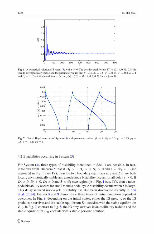
(see Fig. 6). Figure 7 gives the first few global Hopf branches.

123

1286 H. Shu et al.

0 100 200 300 400 500 600 700 8000

0.1

0.2

0.3

0.4

0.5

Fig. 6 A numerical solution of System (3) with τ = 6. The positive equilibrium E∗ ≈ (0.11, 0.41, 0.48) islocally asymptotically stable and the parameter values are: β1 = 6, β2 = 3.5, γ1 = 0.19, γ2 = 0.8, α = 1and β3 = 1. The initial condition is: (x(s), y(s), z(0)) = (0.19, 0.5, 0.3) for s ∈ [−6, 0]

0 5 10 15 20 250

0.05

0.1

0.15

0.2

0.25

0.3

0.35

0.4

0.45

Fig. 7 Global Hopf branches of System (3) with parameter values: β1 = 6, β2 = 3.5, γ1 = 0.19, γ2 =0.8, α = 1 and β3 = 1

4.2 Bistabilities occurring in System (3)

For System (3), three types of bistability mentioned in Sect. 1 are possible. In fact,it follows from Theorem 5 that if D1 > 0, D2 > 0, D3 > 0 and 1 < R1 < 3 (seeregion (i) in Fig. 1 case IV), then the two boundary equilibria E10 and E01 are bothlocally asymptotically stable and a node-node bistability occurs for all delay τ ≥ 0. IfD1 > 0, D2 > 0, D3 > 0 and 3 < R1 (see region (j) in Fig. 1 case IV), then a node-node bistability occurs for small τ and a node-cycle bistability occurs when τ is large.This delay induced node-cycle bistability has also been discovered recently in Shuet al. (2014). Figures 8 and 9 demonstrate these types of initial condition dependentoutcomes. In Fig. 8, depending on the initial states, either the IG prey, y, or the IGpredator, z survives and the stable equilibrium E01 coexists with the stable equilibriumE10. In Fig. 9, contrast to Fig. 8, the IG prey survives in an oscillatory fashion and thestable equilibrium E01 coexists with a stable periodic solution.

123

A Delayed IGP Model 1287

00.2

0.40.6

0.8

0

0.5

1

1.50

0.5

1

1.5

Fig. 8 Node-node bistabilities. The curves are numerical solutions of System (3) with parameter valuesβ1 = 0.5, β2 = 1.2, γ1 = 0.19, γ2 = 0.8, α = 0.5, β3 = 0.5 and τ = 3. For this set of parameters, theresulting (R1,R2) is located in the region (i) of Fig. 1 case IV. The two initial conditions are (x0, y0, z(0)) =(0.29, 1, 0.10) (the green solution trajectory) and (x0, y0, z(0)) = (0.7667, 0.010, 0.4333) (the blue solu-tion trajectory)

00.2

0.40.6

0.8

0

0.5

1

1.50

0.5

1

1.5

Fig. 9 Node-cycle bistabilities. The curves are numerical solutions of System (3) with parameter valuesβ1 = 1, β2 = 1.5, γ1 = 0.19, γ2 = 0.8, α = 1, β3 = 0.25 and τ = 3. For this set of parameters,the resulting (R1,R2) is located in the region (j) of Fig. 1 case IV and τ = 3 > τ0 ≈ 2.07 (E10 isunstable). The two initial conditions are (x0, y0, z(0)) = (0.29, 0.505, 0.15) (the green solution trajectory)and (x(s), y(s), z(0)) = (0.6333, 0.10, 0.5667) (the blue solution trajectory) for s ∈ [−3, 0]

It is seen in Fig. 4 that after a finite number of stability switches, the unique positiveequilibrium becomes unstable for any τ > τ2 ≈ 9.601 and there may exist twoHopf branches when τ is in some intervals, for example, there are two branches forτ ∈ (τ3, τ4) ∪ (τ5, τ6). This suggests that two stable periodic solutions may coexistleading to the occurrence of a bistability involving two periodic solutions. Figure 10demonstrates such a bistability. In Fig. 10, we observe two stable periodic solutionsobtained from two sets of initial conditions. To clearly display the two stable periodicsolutions, we simulate the solutions up to t = 5,000 and omit the initial transitions.

4.3 Chaos

Besides the aforementioned three types of bistability, after a finite number of stabilityswitches the unique positive equilibrium becomes unstable and the bifurcated periodic

123

1288 H. Shu et al.

00.2

0.40.6

0.8

0

0.5

1

1.50

0.5

1

1.5

*

Fig. 10 Cycle-cycle bistabilities. The curves are numerical solutions of System (3) with parameter valuesβ1 = 3.2, β2 = 2, γ1 = 0.19, γ2 = 0.8, α = 1, β3 = 1 and τ = 31. For this set of parameters, theresulting (R1,R2) is located in the region (c) of Fig. 1 case II, the parameter pair (β1, β2) is located in theregion R(iii) of Fig. 3 and τ ∈ (τ5, τ6). Two sets of initial conditions are (x0, y0, z(0)) = (0.6, 0.8, 0.4)(the green solution trajectory) and (x0, y0, z(0)) = (0.2, 0.15, 0.13) (the blue solution trajectory)

0 5 10 15 20 250

0.1

0.2

0.3

0.4

0.5

Fig. 11 Bifurcation diagram of System (3) with parameter values β1 = 6, β2 = 3.5, γ1 = 0.19, γ2 =0.8, α = 1 and β3 = 1, which are located in Region R(vii) of Fig. 3

solutions may be unstable (see Fig. 7). Complex dynamics become possible whenneither a positive equilibrium nor a periodic solution is stable.We use parameter valuesfor Fig. 7 and let the delay τ be the bifurcation parameter to obtain the bifurcationdiagram in Fig. 11. As shown in Fig. 11, there are windows for the delay τ in whichthe solutions of System (3) behave chaotically. For instance, we take τ = 10 and usetwo sets of undistinguishable initial conditions to obtain chaotic attractors in Fig. 12(initial transitions are omitted).

5 Summary and discussion

In this paper we have considered a rather simple intraguild predation model, System(3), that incorporates a reaction delay in the growth of IG prey. For this model, we haveestablished stability and instability results of the equilibria, obtained the critical values

123

A Delayed IGP Model 1289

00.2

0.40.6

0.8

0

0.5

1

1.50

0.5

1

1.5

Fig. 12 Chaotic attractors of System (3) with parameter values: β1 = 6, β2 = 3.5, γ1 = 0.19, γ2 =0.8, α = 1, β3 = 1 and τ = 10. Two sets of initial conditions are used: a (x0, y0, z(0)) = (0.201, 0.5, 0.3)(the red trajectory); b (x0, y0, z(0)) = (0.19, 0.5, 0.3) (the blue trajectory)

at which Hopf bifurcations occur and derived criteria to determine the occurrence andnumber of stability switches. Our results show that, unlikemany predator–preymodelswhere delay has a destabilizing effect and induces oscillations, or many competitionmodels where delay does not induce oscillations, delay in predator–prey relation andcompetition combined intraguild predation models promotes very complex dynamics.If the positive equilibrium of the non-delayed model (τ = 0 in System (3)) is stable,then the timedelay can destabilize the stable positive equilibrium inducing oscillations;if the positive equilibrium is unstable and oscillations are observed in the non-delayedmodel, then the time delay can have a stabilizing role, and as the delay increases, theoscillations disappear and the positive equilibrium gains its stability (Figs. 5, 6). Afterundergoing a finite number of stability switches, when the delay is sufficiently large,the positive equilibrium becomes unstable and oscillations are observed again.

We have shown that delay can induce a variety of bistabilities involving equilibriaand periodic solutions. In particular, a cycle-cycle bistability involves two stable peri-odic solutions. There are regimes in which chaotic behavior can also be induced bydelay. Biologically, possible outcomes include: (i) in the regime where E1 is (glob-ally) stable (Theorem 2), both IG prey and IG predator become extinct; (ii) in theregime that only one boundary equilibrium exists, then either IG prey excludes IGpredator (the case where only E10 exists) or IG predator excludes IG prey (the casewhere only E01 exists); (iii) in the case of node-node bistability, two stable equilibriacoexist allowing for alternative stable equilibria and the outcome is initial conditiondependent; (iv) in the case of node-cycle bistability, either IG predator excludes IGprey and the IG predator population maintains around a constant level (E01 is sta-ble) or IG prey excludes IG predator, but the IG prey population exhibits fluctuations(E10 is unstable and a Hopf bifurcation occurs at E10); (v) in the case of cycle-cyclebistability, coexistence of alternative periodic states occurs, both IG predator and IGprey coexist and undergo sustained fluctuations, and the magnitude of fluctuations areinitial condition dependent; (vi) in the case of chaos, both IG prey and IG predatorcoexist and exhibit irregular oscillations. In addition, the population sizes are sensitiveto the initial conditions.

123

1290 H. Shu et al.

Appendix A:Distribution of the zeros of a first degree exponential transcendentalpolynomial

Lemma 6 Consider the transcendental polynomial given by

g1(λ) = λ + a − be−λτ , (30)

where a > 0, b > 0, τ ≥ 0. For the distribution of the zeros of g1(λ), we have

Case (i): a < b. Then g1(λ) admits one positive real zero and all other zeros arecomplex numbers;

Case (ii): a = b. Then λ = 0 is the only real zero of g1(λ) and all other zeros ofg1(λ) are complex numbers with negative real parts;

Case (iii): a > b. Then g1(λ) has a unique negative real zero, and all other zeroshave negative real parts.

For λ ∈ R, g′1(λ) = 1 + bτe−λτ > 0 and hence g1(λ) is increasing in λ. Thus the

conclusion of case (i) follows easily from g1(0) = a − b < 0.Now we consider case (ii): a = b. Clearly, λ = 0 is the only real zero of g1(λ) and

all other zeros must be complex numbers. Suppose to the contrary that λ = μ + iω isa zero of g1(λ) satisfying μ ≥ 0 and ω > 0. That is, μ + iω + a − a(e−μτ−iωτ ) = 0,which implies |μ + a + iω| = |ae−μτ e−iωτ |. Thus

a2 < a2 + ω2 ≤ (μ + a)2 + ω2 = a2e−2μτ ≤ a2.

A contradiction. Therefore, the conclusion of (ii) holds.Next we consider case (iii). Note that g1(0) = a − b > 0 and g1(−∞) = −∞.

Clearly, the only real zero of g1(λ) must be negative and all other zeros of g1(λ) arecomplex numbers. Suppose that λ = μ+ iω is a zero of g1(λ) with μ ≥ 0 and ω > 0.Then it follows from g1(μ + iω) = 0 that

μ + a = be−μτ cosωτ.

This yields b < μ + a = be−μτ cosωτ ≤ b, a contradiction. Thus the conclusion of(iii) holds and the proof is complete.

Appendix B: Distribution of the zeros of a general transcendental polynomial

In this section we consider the transcendental characteristic equations of the form

H(λ)(P(λ) + Q(λ)e−λτ ) = 0, (31)

where H, P and Q are polynomials with real coefficients and the degree of P is largerthan that of Q. In particular, we are interested in characteristic polynomials arisingfrom the stability analysis of delay-differential equations such as Eq. (3). Without lossof generality, we may assume P and Q have no zeros in common. We further assume

123

A Delayed IGP Model 1291

that H has no zeros with zero real part. In the following, we follow the approach ofCooke and van den Driessche (1986) and summarize their results in our setting.

We regard the time delay, τ , as the bifurcation parameter, and we are only interestedin τ ≥ 0. When τ = 0, the roots of Eq. (31) consist of the zeros of H and (P + Q).For τ > 0, a simple argument shows that as τ changes, any changes in the number ofroots of Eq. (31) with positive real part correspond to pairs of roots crossing into or outof the right half plane. If the transcendental equation Eq. (31) arises as a characteristicequation of a delay differential equation, then these crossings correspond to Hopfbifurcations of solutions in the delay differential equations.

Substituting λ = iω (ω > 0) into Eq. (31), we obtain

F(ω) = |P(iω)|2 − |Q(iω)|2 = 0, (32)

and

τ = 1

ωarg (−Q(iω)/P(iω)). (33)

If ω satisfies Eq. (32) then Eq. (33) defines a sequence of delays, 0 ≤ τ0 < τ1 < . . . ,spaced at intervals τ j+1−τ j = 2π/ω, j = 0, 1, 2, . . . . Since P and Q are polynomialswith real coefficients, F is an even polynomial, and we can define a polynomial Gsuch that F(ω) = G(ω2). Hence, in order for λ = iω to be a nonzero root of Eq. (31),the equation G(u) = 0 must have at least one positive root. In the case where thisroot is simple, we can further show that there is a sequence of Hopf bifurcations as τ

increases.

Lemma 7 Suppose an equilibrium solution of a system of delay-differential equationshas a characteristic equation of the form Eq. (31) with P and Q polynomials. DefineG(u) = |P(i

√u)|2 −|Q(i

√u)|2. If uk > 0 is a simple zero of G, then as τ increases,

the equilibriumundergoes a series ofHopf bifurcations at values of τ kj given byEq. (33)with ω = ωk = √

uk. The associated pair of eigenvalues crosses the imaginary axisfrom left to right if G ′(ω2

k ) > 0, or right to left if G ′(ω2k ) < 0. If G has no positive

zeros, then the number of roots of Eq. (31) with positive real part is independent of τ .

Proof Suppose uk is a simple zero of G, let ωk = √uk , and let τ kj be the sequence

defined by

τ kj = 1

ωkArg (−Q(iωk)/P(iωk)) + 2π j

ωk, j = 0, 1, 2, . . . (34)

where the range of Arg is taken to be the interval [0, 2π). Thus we obtain a sequenceof critical values, τ kj , j = 0, 1, . . . , for τ , at which Eq. (31) admits a pair of simplepurely imaginary roots, ±iωk . These critical values are Hopf bifurcation values if thetransversality condition is further satisfied. Differentiating Eq. (31) with respect to τ ,one gets (

dλ

dτ

)−1

= − P ′(λ)eλτ + (Q′(λ) − τQ(λ)

)λQ(λ)

. (35)

123

1292 H. Shu et al.

Evaluating this expression at the root λ = iωk with τ = τ kj yields

(dλ

dτ

)−1∣∣∣∣∣(λ=iωk ,τ=τ kj )

= P ′(iωk)

iωk P(iωk)− Q′(iωk)

iωk Q(iωk)+ τ kj

iωk

and it follows from the definitions of F and G that

sgn

⎛⎝Re

(dλ

dτ

)−1∣∣∣∣∣(λ=iωk ,τ=τ kj )

⎞⎠ = sgn

(G ′(ω2)

).

Note that for any nonzero complex number λ, sgn(Re(λ)) = sgn(Re( 1λ)). This shows

that

sgn

(d

dτRe(λ)

∣∣∣∣(λ=iωk ,τ=τ kj )

)= sgn

(G ′(uk)

). (36)

Since uk was assumed to be a simple zero of G, with G ′(uk) = 0, the transversalitycondition is satisfied at each τ kj . Hence, Hopf bifurcations occur at the critical values.

Further, if G ′(ω2k ) > 0, then the eigenvalues cross the imaginary axis from left to

right, and the dimension of the unstable manifold increases by two, leading to aloss of stability or continued instability. If, on the other hand, G ′(ω2

k ) < 0, then thedimension of the unstable manifold decreases by two, possibly leading to the stabilityof the equilibrium. ��

In the case where G arises from a characteristic equation of a delay-differentialequation, the degree of P is larger than the degree of Q. The following result followsimmediately and is useful in ordering the zeros of G.

Lemma 8 Suppose P and Q are polynomials with deg(P) > deg(Q). Further, sup-pose that the leading coefficient of P is one and that P and Q have no common zeros.Then the function G defined by G(u) = |P(i

√u)|2 −|Q(i

√u)|2 is a polynomial with

the same degree as P and leading coefficient one.

If G has more than one positive simple zero then there will be a sequence of Hopfbifurcations associated with each such zero. This leads to the possibility of stabilityswitching as τ increases through the critical values. Denote the positive zeros byuk, k = 1, . . . , n, with uk+1 < uk . By Lemma 7, for each positive simple zero uk ,there is a sequence, {τ kj }∞j=0, defined by Eq. (34), with ωk = √

uk , giving values of τ

at which Hopf bifurcations occur. In the case where all positive zeros of G are simple,the slopes at these zeros will alternate in sign. Specifically, G ′(uk) > 0 for k odd andG ′(uk) < 0 for k even. Hence, by Lemma 7, the Hopf bifurcations are stabilizing ifk is even and destabilizing if k is odd. That is, at τ kj , for k even, a pair of complexeigenvalues cross the imaginary axis from the right hand side to the left hand side (thenumber of eigenvalues with positive real parts is reduced by two), while at τ kj , with kodd, a pair of complex eigenvalues cross the imaginary axis from the left hand side tothe right hand side (the number of eigenvalues with positive real parts is increased by

123

A Delayed IGP Model 1293

two). To characterize the possible stability switches at these bifurcations, we define afunction σ(τ), which gives the number of eigenvalues of Eq. (31) with positive realpart. Define the sequences σ k

j as

σ kj =

{−1, if k is even,

+1, if k is odd.(37)

The function σ is then defined as follows:

σ(τ) = σ0 + 2∑

j,k|τ kj <τ

σ kj , (38)

where σ0 denotes the number of zeros of H(P + Q) with positive real part. Notethat if τ kj = τ lm for some k = l, then there will be more complicated bifurcationsoccurring, but the net change in the number of eigenvalues with positive real parts isstill determined by the jumps in σ(τ).

To simplify the remaining lemmas to be presented in this section, we define severalsets, or conditions.

• Let SH be the condition that all zeros of H have negative real parts.• Let S′

H be the condition that H has at least one zero with a positive real part.• Let SG0 be the condition that G has no nonnegative zeros.• Let SG1 be the condition that G has exactly one simple positive zero and no othernonnegative zeros.

• Let SG2 be the condition that G has at least two simple positive zeros and no othernonnegative zeros, with the further restriction that the critical delays associatedwith these zeros are distinct: specifically, τ kj = τml only if j = l and k = m.

• Let SP be the condition that all zeros of P + Q have negative real parts.• Let S′

P be the condition that P + Q has at least one zero with a positive real part.

Note that the conditions sharing common latin subscripts are mutually exclusive.Hence, combinations of these conditions give rise to twelve possible cases. The con-ditions are not exhaustive; however, when viewed as sets in a parameter space, theirclosure encompases all of parameter space.

Lemma 9 Suppose all the positive zeros of the function G defined in Lemma 8 aresimple, and that G has n such zeros, with n ≥ 1. Denote these positive roots by uk, k =1, . . . , n with uk+1 < uk as described following Lemma 8, and define sequencesτ kj , k = 1, . . . , n by Eq. (34) with ωk = √

uk. Then the following holds for thefunction σ defined by Eq. (38). Either σ(τ) > 0 for all τ ≥ 0, or there are integers jand k such that σ(τ kj ) = 0 and σ(τ) > 0 for all τ > τ kj .

Proof First, note that σ(τ) is a step function with positive jumps at critical values of τcorresponding to odd zeros of G and negative jumps at even zeros of G. If the criticalvalues of τ arising from different zeros overlap, then the jump in σ corresponds to thenet number of roots of Eq. (31) whose real parts change sign as τ increases. Since thespacing between delays in the sequence {τ kj }∞j=0 is 2π/ωk and ωk+1 < ωk , positive

123

1294 H. Shu et al.

jumps of σ(τ) as τ increases are more frequent than negative jumps. Hence, regardlessof the orderings of τ k0 , σ must remain positive after some finite τ . ��Lemma 10 Suppose one of conditions SG1 or SG2 hold, and denote the positive zerosof G and their associated sequences of critical delays as in Lemma 9. Then either

(i) σ(τ) > 0 for all τ ≥ 0, or(ii) there exists a set of N positive real numbers 0 < τ0 < τ1 < · · · < τN−2 ≤ τN−1

such that σ(τ) > 0 for τ ∈ [0, τ0) ∪ (τ1, τ2) . . . (τN−3, τN−2) ∪ (τN − 1,∞)

and σ(τ) = 0 for τ ∈ (τ0, τ1) ∪ (τ2, τ3) . . . (τN−2, τN−1), or(iii) there exists a set of N positive real numbers 0 ≤ τ0 < τ1 < · · · < τN−2 ≤ τN−1

such that σ(τ) > 0 for τ ∈ (τ0, τ1) ∪ (τ2, τ3) . . . (τN−3, τN−2) ∪ (τN − 1,∞)

and σ(τ) = 0 for τ ∈ [0, τ0) ∪ (τ1, τ2) . . . (τN−2, τN−1).

Proof If either S′H or S′

P holds, then σ(0) > 0. In contrast, if both SH and SP hold,then σ(0) = 0. Suppose first that σ(0) > 0. Then either case (a) holds, or there issome τ > 0 for which σ(τ) = 0. Since σ is piecewise constant, there must be a largestdelay, τ0, for which σ(τ) > 0 on [0, τ0). Further, it must be that τ0 = τ kj for some evenk. Note that it must also be that τ0 > 0, since it was assumed that Eq. (31) has zeroswith positive real part for τ = 0 and the zeros of Eq. (31) are continuous functions ofτ . Let τ1 denote the next largest element in the sequences τ kj . Since the critical delays,

τ kj , j = 0, 1, 2, . . . , k = 1, . . . , n are assumed distinct, it follows that τ1 = τ kj forsome k odd, and that σ(τ) = 0 on (τ0, τ1). That is, on the interval (τ0, τ1) there areno zeros of Eq. (31) with positive real part, a pair of zeros crosses from the right tothe left half complext plane as τ increases through τ0, and a pair of zeros crosses fromthe left to the right half complex plane as τ increases through τ1. The process canbe repeated to produce a subset {τ0, . . . , τN−1} of delays satisfying 0 < τ0 < τ1 <

· · · < τN−2 ≤ τN−1 for which σ(τ) > 0 for τ ∈ [0, τ0) ∪ (τ1, τ2) . . . (τN−3, τN−2)

and σ(τ) = 0 for τ ∈ (τ0, τ1) ∪ (τ2, τ3) . . . (τN−2, τN−1). By Lemma 9, there mustbe some positive integer N for which σ(τ) > 0 for τ > τN . We have shown that ifσ(0) > 0, then either case (i) or case (ii) holds. Now suppose σ(0) = 0. By Lemma9 there is some τ > 0 for which σ(τ) > 0. Hence, there must be some largest delay,τ0, for which σ(τ) = 0 for τ ∈ [0, τ0). As before, τ0 = τ kj for some odd k. Note thatin this case, it is possible that τ0 = 0. Now either σ(τ) > 0 for all τ > τ0, or there issome τ > 0 for which σ(τ) = 0. We can thus proceed as before to construct a set ofN critical delays for which case (iii) holds. ��Lemma 11 Suppose an equilibrium solution of a system of delay-differential equa-tions has a characteristic equation of the form (31)with P and Q polynomials. Further,let G be defined as above, and suppose one of the 12 mutually exclusive conditionsdefined above holds. Then the equilibriumwill undergo stability switches at the criticaldelays in one of the following manners.

(a) Under conditions S′H , SH ∩S′

P ∩SG0 or SH ∩S′P ∩SG1, the equilibrium is unstable

for all τ ≥ 0.(b) Under conditions SH ∩ SP ∩ SG0, the equilibrium is locally asymptotically stable

for all τ ≥ 0.

123

A Delayed IGP Model 1295

(c) Under conditions SH ∩ SP ∩ SG1, there is a positive real number τ0 such thatthe equilibrium is locally asymptotically stable for τ ∈ [0, τ0) and unstable forτ > τ0 with τ0.

(d) Under conditions SH ∩ SP ∩ SG2, there is a set of N positive real numbers 0 ≤τ0 < τ1 < · · · < τN−2 ≤ τN−1 such that the equilibrium is locally asymptoticallystable for τ ∈ [0, τ0) ∪ (τ1, τ2) . . . (τN−2, τN−1) and unstable for τ ∈ (τ0, τ1) ∪(τ2, τ3) . . . (τN−1,∞).

(e) Under conditions SH ∩ S′P ∩ SG2, there remain two possibilities. Either the equi-

librium is unstable for all τ ≥ 0, or there exists a set of N positive real numbers0 ≤ τ0 < τ1 < · · · < τN−2 ≤ τN−1 such that the equilibrium is unstablefor τ ∈ [0, τ0) ∪ (τ1, τ2) . . . (τN−2, τN−1) and locally asymptotically stable forτ ∈ (τ0, τ1) ∪ (τ2, τ3) . . . (τN−1,∞).

Proof Anequilibriumof a delay differential equation is locally asymptotically stable ifall of its eigenvalues have negative real part, and unstable if any eigenvalue has positivereal part. Hence, if H has zeros with nonnegative real part, then the equilibrium isunstable. If P + Q has zeros with positive real part, then the equilibrium is unstablefor τ = 0. The equilibrium will be stable for some τ > 0 only if sufficient eigenvaluescross from the left half plane to the right half plane as τ increases. This can onlyoccur under condition SG2, where G has a positive zero for which G ′ is negative. Thisestablishes case (a). For case (b), there are no zeros with positive real part for τ = 0,and since G has no positive zeros, by Lemma 7, there can be no values of τ at whicheigenvalues cross into the right half plane. Hence all eigenvalues must remain in theleft half plane and the equilibrium must remain stable for all τ > 0. For case (c), alleigenvalues have negative real part for τ = 0. By Lemma 8, we may assume G isincreasing through its single positive zero. Then by Lemma 7, a pair of eigenvaluescrosses the imaginary axis from left to right as τ increases through τ0. All subsequentbifurcations as τ increases also involve eigenvalues crossing in the same direction.Hence, the equilibrium remains unstable for all τ > τ0.

The remaining two cases allow for a possibility of stability switches as τ increases.In case (d), the equilibrium is stable for τ = 0. Hence, result (iii) of Lemma 10 musthold. Finally, in case (e), the equilibrium is unstable for τ = 0 and so result (i) or (ii)of Lemma 10 must hold. The existence of stability switches depends on the orderingof smallest critical delays, τ k0 . ��

Appendix C: Distribution of simple positive zeros of cubic polynomials

The local stability and Hopf bifurcation analysis of the positive equilibrium E∗ criti-cally rely on the existence and distribution of positive zeros of the cubic polynomialG(u) defined in Eq. (28). In the literature, there has been some work studying thedistribution of zeros of cubic polynomials. For example, conditions on the existenceand nonexistence of positive zeros of cubic polynomials are given in Ruan and Wei(2001). But, to the best of our knowledge, no detailed conditions have been given inthe literature for the existence of exactly m (m = 0, 1, 2, 3) positive zeros of cubicpolynomials. In what follows, we give a complete description on the distribution ofpositive zeros of cubic polynomials.

123

1296 H. Shu et al.

We consider a cubic polynomial given as

p(x) = x3 + p1x2 + p2x + p3, (39)

where p1, p2, p3 are real numbers. Note that p′(x) = 3x2 + 2p1x + p2, which hasthe discriminant Δ = 4(p21 − 3p2). There are two cases to consider.

Case i: p21 ≤ 3p2, i.e., Δ ≤ 0. In this case, p′(x) ≥ 0 and p(x) is nondecreasing.It is easily seen that p(x) has a unique simple positive zero if and only ifp(0) = p3 < 0 and p(x) has no positive zero if p3 ≥ 0.

Case ii: p21 > 3p2, i.e., Δ > 0. In this case, p′(x) has two zeros, x1 = − p13 −

13

√p21 − 3p2 and x2 = − p1

3 + 13

√p21 − 3p2, and p(x) is increasing for

x ∈ (−∞, x1) ∪ (x2,∞) and decreasing for x ∈ (x1, x2). Depending on therelation between zero and x1 and x2, there are three subcases to consider.Case ii.1: x1 ≤ 0 < x2. In this case, if p(0) = p3 ≤ 0, then p(x) hasexactly one simple positive zero since p(x) is decreasing for x ∈ [0, x2) andincreasing for x > x2 and limx→∞ p(x) = ∞; if p3 > 0, then dependingon the value of p(x2), the cubic polynomial p(x) can have no positive zeroprovided that p(x2) > 0, or one positive zero provided that p(x2) = 0 (notethat this zero is not simple and its multiplicity is 2), or two simple positivezeros provided that p(x2) < 0. Case ii.2: x1 < x2 ≤ 0. In this case, notingthat p(x) is strictly increasing for x > 0, thus if p3 < 0, then p(x) hasexactly one positive zero, which is simple, and if p3 ≥ 0, there is no positivezero for p(x). Case ii.3: 0 < x1 < x2. In this case, if p3 ≥ 0, then p(x1) > 0and as in Case ii.1, the cubic polynomial p(x) has no positive zero providedthat p(x2) > 0, or one positive zero with multiplicity of 2 provided thatp(x2) = 0, or two simple positive zeros provided that p(x2) < 0; if p3 < 0,then p(x) has exactly one positive zero provided that p(x1) < 0, two positivezeros provided that p(x1) = 0; in the case that p(x1) > 0, the polynomialp(x) can have one simple positive zero if p(x2) > 0 is further satisfied, twopositive zeros (one is simple, the other is a repeated zero) if p(x2) = 0, andthree simple positive zeros if p(x2) < 0. Note that for Case ii.3, if p3 < 0,then the result on the distribution of positive zeros of p(x) can be summarizedas: if p(x1)p(x2) > 0, then there is one positive zero, if p(x1)p(x2) = 0,then there are two positive zeros, and if p(x1)p(x2) < 0, then there are threepositive zeros.

Define

cp1(p1, p2) = − p13

− 1

3

√p21 − 3p2, cp2(p1, p2) = − p1

3+ 1

3

√p21 − 3p2 (40)

andΔ3(p1, p2, p3) = p21 p

22 − 4p32 − 4p31 p3 − 27p23 + 18p1 p2 p3. (41)

Note that Δ3(p1, p2, p3) is the discriminant of the cubic polynomial p(x). If p21 >

3p2, then cp1(p1, p2) and cp2(p1, p2) are real numbers satisfying cp1(p1, p2) <

123

A Delayed IGP Model 1297

cp2(p1, p2), and p(x1)p(x2) = − 127Δ3(p1, p2, p3), where x1 = cp1(p1, p2) and

x2 = cp2(p1, p2).As we are only interested in the distributions of simple zeros, the above analysis

gives the following result.

Lemma 12 Consider the cubic polynomial p(x) = x3 + p1x2 + p2x + p3 withpi ∈ R, i = 1, 2, 3, cp1(p1, p2) and cp2(p1, p2) defined in Eq. (40), Δ3(p1, p2, p3)defined in Eq. (41). Then the distribution of simple positive zeros of p(x) is completelydescribed as below.

(i) p(x) has no nonnegative zeros if one of the following conditions is satisfied:(i.a) p21 ≤ 3p2 and p3 > 0;(i.b) p21 > 3p2, cp2(p1, p2) < 0;(i.c) p21 > 3p2, cp2(p1, p2) ≥ 0, p3 < 0 and Δ3(p1, p2, p3) < 0.

(ii) p(x) has one simple positive zero and no other nonnegative zeros if one of thefollowing conditions is satisfied:

(ii.a) p21 ≤ 3p2 and p3 < 0;(ii.b) p21 > 3p2, cp1(p1, p2) ≤ 0 and p3 < 0;(ii.c) p21 > 3p2, 0 < cp1(p1, p2), p3 < 0 and Δ3(p1, p2, p3) < 0.

(iii) p(x) has at least two simple positive zeros and no other zeros with nonnegativereal parts if one of the following conditions is satisfied:

(iii.a) p21 > 3p2, 0 < cp2(p1, p2), p3 > 0 and Δ3(p1, p2, p3) > 0;(iii.b) p21 > 3p2, 0 < cp1(p1, p2), p3 = 0 and Δ3(p1, p2, p3) > 0.

References

Abrams PA, Fung SR (2010) Prey persistence and abundance in systems with intraguild predation andtype-2 functional responses. J Theor Biol 264(3):1033–1042

Arim M, Marquet PA (2004) Intraguild predation: a widespread interaction related to species biology. EcolLett 7(7):557–564

Castillo-Chavez C, Thieme HR (1995) Asymptotically autonomous epidemic models. In: Arino O (ed)Mathematical population dynamics: analysis of heterogeneity, I. Theory of epidemics. Wuerz, Canada

Cooke KL, van den Driessche P (1986) On zeroes of some transcendental equations. Funkcialaj Ekvacioj29:77–90

Drolet D, Barbeau MA, Coffin MRS, Hamilton DJ (2009) Effect of the snail Ilyanassa obsoleta (say) ondynamics of the amphipod Corophium volutator (pallas) on an intertidal mudflat. J ExpMar Biol Ecol368(2):189–195

Engelborghs K, Luzyanina T, Samaey G (2001) DDE-BIFTOOL v. 2.00: a matlab package for bifurca-tion analysis of delay differential equations. Tech. Rep. TW-330, Department of Computer Science,K.U.Leuven, Leuven, Belgium

Engelborghs K, Luzyanina T, Roose D (2002) Numerical bifurcation analysis of delay differential equationsusing DDE-BIFTOOL. ACM Trans Math Softw 28(1):1–21

Fan G, Wolkowicz GSK (2010) A predator–prey model in the chemostat with time delay. Int J Differ Equ.doi:10.1155/2010/287969

Fedriani JM, Fuller TK, Sauvajot RM, York EC (2000) Competition and intraguild predation among threesympatric carnivores. Oecologia 125(2):258–270

Freeze M, Chang Y, Feng W (2014) Analysis of dynamics in a complex food chain with ratio-dependentfunctional response. J Appl Anal Comput 4(1):69–87

Hale JK, Verduyn Lunel SM (1993) Introduction to functional differential equations, vol 99. Springer,Berlin

Hall RJ (2011) Intraguild predation in the presence of a shared natural enemy. Ecology 92(2):352–361

123

1298 H. Shu et al.

Hickerson CAM, Anthony CD,Walton BM (2005) Edge effects and intraguild predation in native and intro-duced centipedes: evidence from the field and from laboratorymicrocosms.Oecologia 146(1):110–119

Holt RD, Polis GA (1997) A theoretical framework for intraguild predation. Am Nat 149:745–764Hsu SB, Ruan S, Yang TH (2013) On the dynamics of two-consumers-one-resource competing systemswith

Beddington-DeAngelis functional response. Discrete Cont Dyn-B 18(9):2331–2353. doi:10.3934/dcdsb.2013.18.2331

Hsu SB, Ruan S, Yang TH (2015) Analysis of three species Lotka–Volterra foodwebmodels with omnivory.J Math Anal Appl (to appear)

Kang Y, Wedekin L (2013) Dynamics of a intraguild predation model with generalist or specialist predator.J Math Biol 67:1227–1259

Kuang Y (1993) Delay differential equations: with applications in population dynamics. Academic Press,New York

Li MY, Lin X, Wang H (2014) Global Hopf branches and multiple limit cycles in a delayed Lotka–Volterrapredator–prey model. Discrete Cont Dyn-b 19(3):747–760

Lucas É (2005) Intraguild predation among aphidophagous predators. Eur J Ent 102(3):351MacDonald N (1978) Time lags in biological models, lecture notes in biomathematics, vol 27. Springer,

New YorkMaiti A, Pal AK, Samanta GP (2008) Effect of time-delay on a food chain model. Appl Math Comp

200(1):189–203Pimm SL, Lawton JH (1978) On feeding on more than one trophic level. Nature 275(5680):542–544Polis GA, Holt RD (1992) Intraguild predation: the dynamics of complex trophic interactions. Trends Ecol

Evol 7(5):151–154Polis GA, Myers CA, Holt RD (1989) The ecology and evolution of intraguild predation: potential com-

petitors that eat each other. Ann Rev Ecol Syst 20:297–330Ruan S (2009) On nonlinear dynamics of predator-prey models with discrete delay. Math Mod Nat Phen

4(02):140–188Ruan S, Wei J (2001) On the zeros of a third degree exponential polynomial with applications to a delayed

model for the control of testosterone secretion. Math Med Biol 18(1):41–52Shi J (2013) Absolute stability and conditional stability in general delayed differential equations. In:

Advances in interdisciplinary mathematical research, Springer proceedings in mathematics & sta-tistics, vol 37. Springer, New York, pp 117–131

Shu H, Wang L, Watmough J (2014) Sustained and transient oscillations and chaos induced by delayedantiviral immune response in an immunosuppressive infection model. J Math Biol 68:477–503

SongY,Wei J (2005) Local Hopf bifurcation and global periodic solutions in a delayed predatorprey system.J Math Anal Appl 301(1):1–21. doi:10.1016/j.jmaa.2004.06.056

TanabeK,Namba T (2005)Omnivory creates chaos in simple foodwebmodels. Ecology 86(12):3411–3414Velazquez I, Kaplan D, Velasco-Hernandez JX, Navarrete SA (2005) Multistability in an open recruitment

food web model. Appl Math Comput 163(1):275–294Verdy A, Amarasekare P (2010) Alternative stable states in communities with intraguild predation. J Theor

Biol 262(1):116–128. doi:10.1016/j.jtbi.2009.09.011Wangersky PJ, CunninghamWJ (1957) Time lag in prey–predator population models. Ecology 38(1):136–

139Wolkowicz GSK, Xia H (1997) Global asymptotic behavior of a chemostat model with discrete delays.

Siam J Appl Math 57(4):1019–1043Xiao D, Ruan S (2001) Global analysis in a predator–prey system with nonmonotonic functional response.

Siam J Appl Math 61(4):1445–1472Yamaguchi M, Takeuchi Y, Ma W (2007) Dynamical properties of a stage structured three-species model

with intra-guild predation. J Comput Appl Math 201(2):327–338

123