Federal Reserve Bank of New York

Staff Reports

Deflationary Shocks and Monetary Rules:

An Open-Economy Scenario Analysis

Douglas Laxton

Papa N’Diaye

Paolo Pesenti

Staff Report no. 267

December 2006

This paper presents preliminary findings and is being distributed to economists

and other interested readers solely to stimulate discussion and elicit comments.

The views expressed in the paper are those of the authors and are not necessarily

reflective of views at the Federal Reserve Bank of New York or the Federal

Reserve System. Any errors or omissions are the responsibility of the authors.

Deflationary Shocks and Monetary Rules: An Open-Economy Scenario Analysis

Douglas Laxton, Papa N’Diaye, and Paolo Pesenti

Federal Reserve Bank of New York Staff Reports, no. 267

December 2006

JEL classification: E17, E52, F41

Abstract

The paper considers the macroeconomic transmission of demand and supply shocks in

an open economy under alternative assumptions about whether the zero interest rate

floor (ZIF) is binding. It uses a two-country general-equilibrium simulation model

calibrated to the Japanese economy relative to the rest of the world. Negative demand

shocks have more prolonged and conspicuous effects on the economy when the ZIF is

binding than when it is not binding. Positive supply shocks can actually extend the

period of time over which the ZIF may be expected to bind. Economies that are more

open hit the ZIF for a shorter period of time, and with less harmful effects. The

implications of deflationary supply shocks depend on whether the shocks are

concentrated in the tradables or the nontradables sector. Price-level-path targeting rules

are likely to provide better guidelines for monetary policy in a deflationary environment,

and have desirable properties in normal times when the ZIF is not binding.

Key words: deflation, monetary policy rules, zero interest rate floor

Laxton: International Monetary Fund (e-mail: dlaxton@imf.org). N’Diaye: International

Monetary Fund (e-mail: pndiaye@imf.org). Pesenti: Federal Reserve Bank of New York (e-mail:

paolo.pesenti@ny.frb.org). The authors thank Shin-ichi Fukuda, Takeo Hoshi, Takatoshi Ito,

Andy Rose, Kazuo Ueda, Tsutomu Watanabe, Alessandro Zanello, and conference participants at

the 18th Annual TRIO Conference in Tokyo for helpful suggestions. They also thank Hope

Pioro, Susanna Mursula, and Chris Tonetti for invaluable assistance. The views expressed in this

paper are those of the authors and do not necessarily reflect the position of the International

Monetary Fund, its Executive Board, management, or any member government, or the position

of the Federal Reserve Bank of New York or the Federal Reserve System.

1 Introduction

In recent years, quite a few research agendas have sought to pin down the causes of de�ation,mostly focusing on whether falling prices are the result of structural factors or insu¢ cientaggregate demand. In a nutshell, structural factors such as productivity improvements inthe manufacturing sector are deemed to be responsible for worldwide disin�ation, whileweaknesses in demand are typically assumed to be accompanied by di¢ culties in providingmonetary policy stimulus when interest rates hit the zero interest rate �oor (ZIF). Speci�-cally, the two views above have represented recurrent themes in both the policy and academicdebate on the performance of the Japanese economy over the last 15 years.1

This paper does not take a speci�c view about the historical contribution of demandand supply factors in the evolution of prices in Japan, nor makes any normative or policystatements on the best course of action in the near future. Rather, it makes the simple pointthat a country facing de�ationary risks would bene�t from an integrated approach involvingmacroeconomic policies able to respond appropriately to adverse aggregate demand shocksand deal with the consequences of eventual expansions in supply. Such framework wouldnot only eliminate de�ation in the short run, but also guard against falling into liquiditytraps in the future.Using a 2-country simulation model calibrated to the Japanese economy, the paper car-

ries out a scenario analysis to illustrate possible di¢ culties in dealing with both demandand supply shocks when the ZIF is binding. It shows that the e¤ects of negative demandshocks on the economy become more protracted and startling when the ZIF is binding thanduring normal times when it is not binding. It also shows that positive supply shocks (e.g.shocks that raise potential output) can extend the period of time during which the ZIF isexpected to be binding, increasing the economy�s vulnerability to adverse demand shocks.In addition, the paper comments on the relative bene�ts of alternative monetary rules in ade�ationary environment, including price level targeting, in�ation-targeting, and price-level-path targeting rules. The results indicate that price-level-path targeting rules are likely toprovide better guidelines for monetary policy because they are more robust in a de�ationaryenvironment, and � when appropriately designed � have desirable properties in normaltimes when the ZIF is not binding.Throughout the paper we deliberately emphasize the implications of trade and �nancial

openness on the e¤ectiveness of monetary rules in a de�ationary environment. This is not torestate the point made elsewhere (e.g. McCallum 2000 and Svensson 2001) that in an open-economy context policymakers can escape a liquidity trap by engineering the appropriatepath for the exchange rate. Rather, we show that in the face of negative demand shocks,more open economies are less vulnerable to the problems associated with the ZIF: otherthings being equal, they hit the ZIF for a shorter period of time, and with less harmfule¤ects. In addition, openness can reverse the sign of the short-term response of real exchangerates to shocks. With low openness, de�ation results in a very high and persistent rise in realinterest rates that strengthens the home currency in real terms. In contrast, with greateropenness real interest rates are not expected to increase or even remain at a high level fora long time, and the real exchange rate depreciates on impact.Finally, the mechanism of transmission of de�ationary supply shocks is signi�cantly

1See e.g. Callen and Ostry (2003), Eggertsson and Woodford (2003, 2004), and Hunt and Laxton(2001, 2003), Hayami (2001), Hayashi and Prescott (2004), Krugman (1998a, 1998b), McCallum (2000),and Svensson (2001).

1

a¤ected by whether they are concentrated in the tradables or the nontradables sector. Inboth cases the appropriate policy response is to reduce interest rates when it is possible(either now or in the future). However, when the shock is concentrated in the nontradablessector it results in a depreciation of the real exchange rate and stronger growth in the shortrun, reducing the period of time over which the ZIF is binding relative to the case in whichthe productivity shock is concentrated in the tradables sector.The remainder of this paper is organized as follows. Sections 2 and 3 describe the basic

theoretical structure of the model and its calibration. Section 4 discusses the relative prop-erties of price-level-path targeting rules. Section 5 then provides some illustrative scenariosto support the key arguments in the paper. The last section concludes by providing a briefdiscussion of possible future extensions.

2 The structure of the model

This section sets up a general equilibrium two-country model.2 The home country (indexedby H) is calibrated on Japanese data, while F (the �foreign�country) indexes the rest of theworld. The size of the world economy is normalized to 1, with sH denoting the size of thehome country and sF = 1� sH the size of the rest of the world.There is a common trend for the world economy, whose gross rate of growth between

time t and time � is denoted gt;� . Each period t represents a quarter. All quantity variablesin the model are expressed in detrended terms.In each country, there are households, �rms, and a government. Households consume a

nontradable �nal good and supply di¤erentiated labor inputs to �rms. Firms produce �nalgoods, tradable and nontradable intermediate goods, and provide intermediation services.The public sector consumes domestic goods and services, �nanced through lump-sum tax-ation, and manages short-term interest rates. These sectors are described in more detailbelow.

2.1 Final goods

In each country there is a continuum of symmetric �rms producing two �nal goods, theconsumption good (A) and the investment good (E), under perfect competition. The pro-duction function of the representative �rm in the A sector is:

AHt1� 1

"HA =

�1� HA

� 1

"HA NH

A;t

1� 1

"HA

+ HA

1

"HA

��HA

1

�HA QHA;t

1� 1

�HA +

�1� �HA

� 1

�HA MH

A;t

1� 1

�HA

�� �HA�HA�1

��1� 1

"HA

�(1)

Three intermediate inputs are used in the production of the consumption good: a basketof nontradable goods (NA), a basket of domestic tradable goods (QA), and a basket ofimported goods (MA). The elasticity of substitution between tradables and nontradables is"A, and the elasticity of substitution between domestic and imported tradables is �A.

2Our framework is a variant of the multi-country model presented in the Appendix of Faruqee, Lax-ton, Muir and Pesenti (2006), and is nested within the Global Economy Model (GEM) developed at theInternational Monetary Fund.

2

The Consumer Price Index (CPI) is the price of one unit of A. The (gross) in�ationrate is de�ned as:

�Ht;� =CPIH�CPIHt

(2)

As a convention throughout the model, A is the numeraire of the economy and all nationalprices are expressed in terms of domestic units of consumption, that is as ratios of CPI.Cost minimization determines �rms�demands for intermediate inputs as:

NHA;t =

�1� HA

�pHN;t

�"HAAHt (3)

QHA;t = HA �HA p

HQ;t

��HA pHXA;t�HA�"

HAAHt (4)

MHA;t = HA

�1� �HA

�pHMA;t

��HA pHXA;t�HA�"

HAAHt (5)

where pN , pQ, and pMA are the relative prices of the inputs in terms of consumptionbaskets, and pXA is the cost-minimizing price of the composite basket of domestic andforeign tradables:

pHXA;t =��HA p

HQ;t

1��HA +�1� �HA

�pHMA;t

1��HA� 1

1��HA (6)

The consumption good sector in the rest of the world and the investment good sector inboth countries are similarly characterized, with self-explanatory changes in notation.

2.2 Demand for intermediate goods

There are di¤erent varieties (brands) of intermediate inputs that are produced in monopo-listically competitive markets. In each country there are two kinds of intermediate goods,tradables and nontradables. Each type is de�ned over a continuum of mass equal to thecountry size. In what follows �HN > 1 denotes the elasticity of substitution between inter-mediate nontradables in the baskets NH

A and NHE , while �

HT > 1 is the analogous elasticity

for the baskets QHA and QHE in the home country and MFA and MF

E in the rest of the world(similarly, �FT > 1 is the elasticity associated with the baskets Q

FA, Q

FE , M

HA and MH

E ).It is assumed that imports are subject to adjustment costs that temporarily shrink the

production possibility frontier of the importing �rms. This assumption allows us to modelrealistic dynamics of imports volumes (such as delayed and sluggish adjustment to changesin relative prices). Denoting withMH;F

A exports from the rest of the world F to the A sectorof the home country H, we have:

MHA;t =

�1� �H;FMA;t

�MH;FA;t (7)

The adjustment costs �H;FMA for a representative �rm xH are speci�ed in terms of the �rm�scurrent import share relative to the past observed import share for the sector as a whole.These adjustments costs are zero in steady state. Speci�cally, we adopt the parameteriza-tion:

�H;FMA;t(xH) =

�H;FMA

2

[(MH;FA;t (x

H)=AHt (xH))=

�MH;FA;t�1=A

Ht�1

�� 1]2

1 + [(MH;FA;t (x

H)=AHt (xH))=

�MH;FA;t�1=A

Ht�1

�� 1]2

(8)

Denoting pH;FM the home-currency price of country F�s exports to H, cost minimizationimplies:

pHMA;t(xH) =

pH;FM;t

1� �H;FMA;t(xH)�MH;F

A;t (xH)�0H;FMA;t(x

H)(9)

3

where �0H;FMA (xH) is the �rst derivative of �H;FMA (x

H) with respect to MH;FA (xH). To the

extent that all �rms xH are symmetric within the consumption sector, there will be aunique cost-minimizing import price pHMA. Similar considerations apply to the E sector andthe F country.

2.3 Supply of intermediate goods

The representative nontradable intermediate good in the home country is produced withthe following CES technology:

NHt = ZHN;t

��1� �HKN

� 1

�HN

�`HN;t

�1� 1

�HN + �HKN

1

�HN

��1� sHLC

�KHN;t

�1� 1

�HN

� �HN�HN�1

(10)

Each �rm uses labor (`) and capital (K) to produce N units of its variety. �N > 0 is theelasticity of input substitution, and ZN is a productivity shock common to all producersof nontradables. The expression 1 � sLC denotes the share of households that own andaccumulate capital and rent it to �rms.De�ning as wt and rt the prices of labor and capital, the marginal cost in nontradables

production is:3

mcHN;t =1

ZHN;t

��1� �HKN

� �wHt�1��HN + �HKN �rHt �1��HN� 1

1��HN (11)

and the capital-labor ratio is:

�1� sHLC

� KHN;t

`HN;t=

�HKN1� �HKN

�wHtrHt

��HN(12)

Similar considerations hold for the production of tradables. We denote by T the supply ofthe representative intermediate tradable good. Using self-explanatory notation, we have:

THt = ZHT;t

��1� �HKT

� 1

�HT

�`HT;t�1� 1

�HT + �HKT

1

�HT

��1� sHLC

�KHT;t

�1� 1

�HT

� �HT�HT�1

(13)

2.4 Price setting in the intermediate sector

Consider now pro�t maximization in the intermediate nontradables sector of the homecountry. The representative �rm nH sets its nominal price by maximizing the presentdiscounted value of real pro�ts. Nominal rigidities are introduced in the form of adjustmentcosts occurring when the �rm modi�es its prices. Such adjustment costs are measured interms of total pro�ts foregone and denoted �HPN;tfpHt (nH); pHt�1(nH)g.The price-setting problem of the �rm can be characterized as:

maxpt(nH)

Et

1X�=t

DHt;��

Ht;�gt;�

�pH� (n

H)�mcHN;�� pH� (nH)

pHN;�

!��HNNH�

�1� �HPN;� (nH)

�(14)

where DHt;� (with D

Ht;t = 1) is the appropriate discount rate, to be de�ned below. As real

variables are detrended and prices are de�ated by CPI, eq. (14) includes �Ht;� , the in�ation

3Following the notational convention regarding prices, mct, wt and rt denote marginal costs, wages andrental rates in consumption units.

4

rate between time t and time � , and gt;� , the rate of growth of the world trend betweent and � . Demand for the variety nH is a function of its relative price pH(nH)=pHN (withelasticity �HN ) and total consumption of nontradables, N

H .The speci�c parameterization of the adjustment cost �HPN allows the model to engender

realistic nominal dynamics, including in�ation inertia:

�HPN;t(nH) � �HPN

2

�Ht�1;t

pHt (nH)=pHt�1(n

H)

�HN;t�2;t�1� 1!2

(15)

The adjustment cost is related to changes in the price of the nontradable good nH relativeto the past (quarterly) in�ation rate observed in the nontradables sector, �HN;t�2;t�1. Un-derlying this speci�cation is the notion that �rms should not be penalized when their pricechanges are indexed to some (publicly observable) benchmark such as the past in�ation ratefor the sector as a whole.4

As �rms are symmetric and charge the same equilibrium price pH(nH) = pHN , the �rstorder condition can be written as:

0 =�1� �HPN;t

� hpHN;t

�1� �HN

�+ �HNmc

HN;t

i��pHN;t �mcHN;t

� @�HPN;t@pHN;t

pHN;t

� EtDHt;t+1�

Ht;t+1gt;t+1

�pHN;t+1 �mcHN;t+1

� NHt+1

NHt

@�HPN;t+1@pHN;t

pHN;t (16)

Interpreting the previous equation,5 when prices are fully �exible (�HPN = 0), the optimiza-tion problem collapses to the standard markup rule:

pHN;t =�HN

�HN � 1mcHN;t (17)

where the gross markup is a negative function of the elasticity of input substitution. De-viations from markup pricing occur if �rms are penalized for modifying their prices in theshort term. The speed of adjustment in response to shocks depends on the trade-o¤ betweencurrent and future expected costs, making the price-setting process forward-looking.Similar considerations apply to the price-setting decisions of �rms in the tradables sector,

determining pHQ , pFQ, p

H;FM and pF;HM .6 To the extent that the home country and the rest of

the world represent segmented markets, each �rm needs to set two prices, one for domesticsales and the other for the export market. Without loss of generality, exports are invoiced(and prices are set) in the currency of the destination market. The adjustment costs arespeci�ed as in (15), but with possibly di¤erent parameters in the domestic market andthe export market (respectively �HPQ and �

F;HPM for the home country�s �rms). If the latter

coe¢ cient is relatively large, the prices of home country H�s goods in the foreign marketsF are characterized by signi�cant stickiness in local currency. In this case, the degree towhich exchange rate �uctuations (and other shocks to marginal costs in country H) pass

4More generally, the adjustment cost could be speci�ed relative to any variable that converges asymp-totically to the steady-state in�ation rate. It is worth emphasizing that the adjustment costs are related tochanges in nominal prices. However, the maximization problem can be easily rewritten in terms of relativeprices, as carried out in this section.

5When linearized around the steady state, eq.(16) can be written as a standard new-Keynesian Phillipscurve under full indexation, or ��HN;t = �mc

HN;t + �Et��

HN;t+1, where � =

��HN � 1

��HN=�

HPN .

6See Faruqee, Laxton, Muir and Pesenti (2006) for details.

5

through onto import prices in country F is rather low. If there were no nominal rigiditiesworldwide, export price setting would collapse to a markup rule under the law of one price,and exchange rate pass-through would be full:

pHQ;t = "tpF;HM;t =

�HT�HT � 1

mcHT;t (18)

where " is the CPI-based real exchange rate (an increase in " representing a real depreciationfor the home country H). By choosing an appropriate parameterization for �PM in bothcountries, it is possible to reproduce realistic values for the elasticity of exchange rate pass-through in the short run. In the long run, however, pass-through is full and the law of oneprice holds in both markets.

2.5 Consumer preferences

In each country there is a continuum of households. Some households have access to capitalmarkets, and others do not. Those who don�t have access to capital markets �nance theirconsumption exclusively through their labor income. This type of consumers is referred to as�non-Ricardian�or �liquidity-constrained�, and indexed with LC. In the home country, theyrepresent a share sHLC of domestic households. Those who have access to capital markets arereferred to as �Ricardian�or �forward-looking�, and indexed with FL. In the home country,they represent a share

�1� sHLC

�of domestic households.

The speci�cation of households�preferences uses the Greenwood, Hercowitz and Hu¤man(1988) (GHH) utility function, adjusted for habit formation and preference shocks. Denotingwith WH

t (jH) the lifetime expected utility of the representative household jH in the home

country, we have:

WHt (j

H) � Et1X�=t

�Ht;�g1��t;� uH� ( C

H� (j

H); `H� (jH) ) (19)

where the instantaneous felicity is a function of consumption C and labor e¤ort `:

uHt (jH) = ZHU;t (1�

bHcgt�1;t

) (1� bH`1� � )

�[CHt (j

H)� bHc CHjH ;t�1=gt�1;t1� bHc =gt�1;t

�ZHV;t

1 + �H(`Ht (j

H)� bH` `Hj;t�11� bH`

)1+�H

]1�� (20)

In the expressions above �Ht;� is the discount rate between time t and time � , possiblydi¤erent across countries. The disutility of labor e¤ort is assumed to increase with the globaltrend (hence the term g1��t;� in 19).7 The parameter � in (19) and (20) is the reciprocal ofthe elasticity of intertemporal substitution. The parameter � which a¤ects the curvature oflabor disutility is the reciprocal of the Frisch elasticity.There is habit persistence in consumption with coe¢ cient 0 < bc < 1. The term CjH ;t�1

in (20) is past per-capita consumption of household jH�s peers, (i.e., either forward-lookingor liquidity-constrained agents). Similarly, there is habit persistence in leisure with coe¢ -cient 0 < b` < 1.8 The terms ZU and ZV are preferences shocks. Households�preferences

7Appropriate restrictions are imposed to ensure that utility is bounded. In particular, in steady state wehave �SSg

1��SS < 1 in all countries.

8The instantaneous felicity is normalized such that in a steady state U , UC and U` can all be written asconstant � f(C; `), where f is some function of steady-state consumption and labor e¤ort, independent ofthe habit persistence coe¢ cients.

6

are therefore symmetric within their respective categories but, because of di¤erent referencegroups in habit formation, they are not symmetric across categories.

2.6 Ricardian households

Ricardian households in the home country hold two nominal bonds, denominated in domesticand foreign currency, respectively. The domestic bond is in zero net supply in the homecountry, and only the foreign-currency denominated bond is traded internationally. BHt (j

HFL)

denotes the holdings of the domestic bond by households jHFL, expressed in terms of domesticconsumption units, and BHF;t(j

HFL) that of international bond, expressed in terms of foreign

consumption units. The nominal returns on these bonds are denoted iHt and iFt . They arepaid at the beginning of period t + 1 and known at time t. The two rates are directlycontrolled by their respective national governments.Home agents who take a position in the international bond market must deal with �nan-

cial intermediaries who charge a transaction fee �HBF on sales/purchases of the internationalbond.9 The net �nancial wealth of the home country, expressed in local consumption bas-kets, is therefore:

FHt � (1 + iFt�1)�1� �HBF;t�1

� "tBHF;t�1

�Ft�1;tgt�1;t(21)

The �nancial friction is introduced to guarantee that international net asset positionsfollow a stationary process and the economies converge asymptotically to a well-de�nedsteady state. Speci�cally, we adopt the following functional form:

1� �HBF;t = (1� �HB1expf�HB2("t

�1� sHLC;t

�BHF;t=GDP

Ht � bHF;RAT;SS)g � 1

expf�HB2("t�1� sHLC;t

�BHF;t=GDP

Ht � bHF;RAT;SS)g+ 1

)�Ft�1;t

�Ht�1;t(22)

The term bHF;RAT;SS is the steady-state net asset position of the home country expressedas a ratio of GDPH .10 This variable measures the degree of international exposure that�nancial intermediaries consider appropriate, based on their long-term assessment of theeconomy. In our simulation we set bHF;RAT;SS = 0, as alternative parameterizations leaveour results virtually unchanged.To understand the role played by �HBF , suppose that �

F = �H . In this case, whenthe net asset position of the country is equal to its steady-state level of zero, it must bethe case that �HBF = 0 and the return on the international bond is equal to 1 + iF . Ifinstead home residents are net creditors worldwide, �HBF rises above zero, implying thatthe country�s households lose an increasing fraction of their international bond returns to�nancial intermediaries. By the same token, if the home country is a net debtor worldwide�HBF becomes negative (with a �oor of ��B1), implying that households pay an increasingintermediation premium on their international debt.11 When rates of time preference divergeacross countries and �H 6= �F , the transaction cost is appropriately modi�ed to account forasymmetries in real interest rates across countries. An appropriate parameterization allowsthe model to generate realistic dynamics for net asset positions and current account.

9 In our model it is assumed that all intermediation �rms are owned by the country�s residents, and thattheir revenue is rebated to domestic households in a lump-sum fashion.

10The concept of GDP in our model will be discussed below.

11More generally, the term bHF;RAT;SS could be di¤erent from zero. The above considerations would stillbe valid after reinterpreting the concepts of �net creditor�or �net borrower�in terms of deviations from thesteady-state level.

7

Ricardian households accumulate physical capital which they rent to domestic �rms atthe rate r. The law of motion of capital is:

KHt gt�1;t =

�1� �H

�KHt�1 + �

HI;t�1K

Ht�1 0 < � � 1 (23)

where �H is the country-speci�c depreciation rate of capital. Capital accumulation is subjectto adjustment costs �I . The speci�c functional form we adopt is quadratic and encompassesinertia in investment:

�HI;t �IHtKHt

�1 + ZHI;t

�� �HI1

2

�IHtKHt

���H + gSS � 1

��2� �HI2

2

�IHtKHt

�IHt�1KHt�1

�2(24)

where �I1, �I2 � 0, ZI is a shock to investment demand and gSS is the steady-state growthrate.Labor inputs are di¤erentiated and come in di¤erent varieties (skills). They are de�ned

over a continuum of mass equal to the country size. In what follows H > 1 is the elasticityof substitution among labor inputs in the home country. Each household is the monopolisticsupplier of a speci�c labor input and sets the nominal wage for its speci�c labor variety.The representative Ricardian household jHFL faces a downward-sloping demand for its laborinput as a function of its relative wage wHFL=w

H :

`HFL;t =�1� sHLC

� �wHFL;t=w

Ht

�� H`Ht (25)

where `H is aggregate labor e¤ort in the home country. There is sluggish wage adjustmentdue to resource costs that are measured in terms of the total wage bill. The adjustmentcost is speci�ed as the analog of (15) above, with parameter �HWFL.Ricardian households own all domestic �rms and there is no international trade in claims

on �rms�pro�ts. All pro�ts accruing to shareholders, together with all revenue from nominaland real adjustment as well as revenue from �nancial intermediation are distributed in alump-sum way to all Ricardian households. In addition, all net taxes paid to the governmentare lump-sum.The representative Ricardian household chooses bond holdings, capital and consumption

paths, and sets its nominal wage to maximize its expected lifetime utility (19) subject to itsbudget constraint. The stochastic discount rate DH

t;� is de�ned as:

DHt;� � �Ht;�g

1��t;�

@uHFL;�=@CHFL;�

@uHFL;t=@CHFL;t

1

�Ht;�

1

gt;�(26)

Accounting for the above expressions, the bond-pricing equations are, respectively:

1 =�1 + iHt

�EtD

Ht;t+1 (27)

1 =�1 + iFt

� �1� �HBF;t

�Et�DHt;t+1�

Ht;t+1

�(28)

where �H denotes the rate of nominal exchange rate depreciation in the home country, or:

�Ht;� ="�"t

�Ht;��Ft;�

(29)

In a non-stochastic steady state (27) implies�1 + iHSS

�=�HSS = g�SS=�

HSS , where �

HSS is the

(gross steady-state quarterly) in�ation rate,�1 + iHSS

�=�HSS is the real interest rate, g

HSS

8

is the (gross steady-state quarterly) rate of growth of the world economy, 1=�HSS is therate of time preference, and g�SS=�

HSS is the �natural� rate of the economy.

12 In a non-stochastic steady state the interest di¤erential

�1 + iHSS

�=[�1 + iFSS

� �1� �HBF;SS

�] is equal

to the steady-state nominal depreciation rate of the home currency, and relative purchasingpower parity holds.Optimal capital accumulation is determined according to:

pHE;t

@�HI;t=@�IHt =K

Ht

�Etgt;t+1 = Etf DHt;t+1�

Ht;t+1gt;t+1(r

Ht+1

+pHE;t+1

@�HI;t+1=@�IHt+1=K

Ht+1

� [1� �H + �HI;t+1 � @�HI;t+1

@�IHt+1=K

Ht+1

� IHt+1KHt+1

] ) g (30)

where pHE =@�HI =@

�IH=KH

�can be interpreted as Tobin�s Q. In a non-stochastic steady

state 1 + rHSS=pHE;SS is equal to the sum of the natural real rate g�SS=�

HSS and the rate of

capital depreciation �.13

Finally, the �rst order condition with respect to the nominal wage yields an expressionsimilar to (16) above. In a non-stochastic steady state the real wage of the Ricardian house-hold wHFL is equal to the marginal rate of substitution between consumption and leisure,

�(@uHFL;t=@`HFL;t)=(@uHFL;t=@CHFL;t), augmented by the markup H=� H � 1

�which re-

�ects monopoly power in the labor market.The rest of the world is similarly characterized. However, there are no intermediation

costs in entering the international bond market for the Ricardian households of the F coun-try.

2.7 Liquidity-constrained households

Liquidity-constrained households have no access to capital markets. However, they face adownward-sloping demand for their labor inputs as a function of their relative wage:

`HLC;t = sHLC�wHLC;t=w

Ht

�� H`Ht (31)

As in the case of Ricardian households, they can set optimally their wages using their marketpower, subject to adjustment costs with parameter �HWLC . It is assumed that redistributionpolicies provide to these households the income losses associated with wage adjustment,implying that their consumption level is:

CHFL;t = wHLC;t`HLC;t (32)

and the optimal wage setting process is:

�@uHLC;t=@`

HLC;t

@uHLC;t=@CHLC;t

H

wHLC;t=� H � 1

� �1� �HWLC;t

�+@�HWLC;t

@wLC;twHLC;t (33)

12 International di¤erences in natural rates can arise from asymmetric rates of time preference. They areaccounted for in the de�nition of �B in (22).

13The expectation operator on the left hand side of (30) is needed as shocks to the trend gt;t+1 are notpart of the information set at time t. This is because variables are expressed as deviations from the currenttrend. An alternative speci�cation which expresses variables as deviations from the lagged trend wouldmake little di¤erence.

9

Finally, the wage rate for the whole economy is:

wH 1� Ht = sHLC wH 1� H

LC +�1� sHLC;t

�wH 1� HFL (34)

Similar considerations hold in the F country.

2.8 Government

Public spending is limited to nontradable goods, both �nal and intermediate. In per-capitaterms, GHC is government consumption, GHI is government investment, and GHN denotespublic purchases of intermediate nontradables. Government spending is �nanced throughlump-sum taxationThe governments control the short-term rates iHt and i

Ft . In the home country, monetary

policy encompasses both in�ation and price level targeting and is speci�ed in terms of anannualized interest rate rule of the form:

�1 + iHt

�4=�1 + ineut Ht

�4+ !H�

��Ht�4;t ��HTAR t�4;t

�+ !HP ln

CPIHt

CPIHTAR;t

!(35)

The current interest rate it is a function of the current �neutral�rate ineutt , de�ned as thequarterly nominal interest rate that would prevail if the real interest rate were equal to thenatural rate and in�ation were equal to its target:

1 + ineut Ht ��H 0:25TAR;t�4;t (gt�1;t)

�

�Ht�1;t(36)

The current rate can di¤er from neutral to account for the gap between current year-on-yearin�ation (�Ht�4;t) and its target (�

HTAR t�4;t), as well as the gap between the current price

level CPIHt and its target CPIHTAR;t. The latter is de�ned according to:

�HTAR t;� =CPIHTAR;�CPIHTAR;t

(37)

All nominal prices are normalized at the initial time t = 0 such that CPI0 = CPITAR;0 = 1.We refer to the expression (35) as a Price-Level-Path Targeting (PLPT) rule when the targetrate of in�ation is positive and a Price-Level Targeting (PLT) rule when the target rate ofin�ation is zero.In general, the rule (35) could be modi�ed to include policy responses to a set of other

variables (such as output gap, output growth rate, exchange rate, current account etc.)expressed as deviations from their targets. In a steady state when all targets are reached itmust be the case that the real interest rate is equal to the �natural�rate of the economy, afunction of the long-term growth rate and the discount rate:

1 + iHSS = 1 + ineut HSS =

�H 0:25SS g�SS�HSS

=�SSg

�SS

�SS: (38)

In the rest of the world monetary policy is similarly speci�ed, but the interest rate ruleis assumed to only respond to deviations of in�ation from the target.

10

2.9 Market clearing

The model is closed by imposing the following resource constraints and market clearingconditions.The resource constraint in the nontradables sector is:

NHt = NH

A;t +NHE;t +G

HN;t (39)

The resource constraint in the tradables sector in the home country is:

THt = QHA;t +QHE;t +

sF

sH

�MF;HA;t +M

F;HE;t

�(40)

and similarly, in the rest of the world:

TFt = QFA;t +QFE;t +

sH

sF

�MH;FA;t +M

H;FE;t

�(41)

The resource constraints in the labor and capital markets are:

KHt = KH

T;t +KHN;t (42)

`Ht = `HN;t + `HT;t (43)

The �nal good A can be used for private (by both liquidity-constrained and forward-looking households) or public consumption:

AHt = CHt +GHC;t = sHLC;tC

HLC;t +

�1� sHLC;t

�CHFL;t +G

HC;t (44)

and similarly for the investment good E:

EHt =�1� sHLC;t

�IHt +G

HI;t (45)

All pro�ts and intermediation revenue accrue to Ricardian households. Market clearing inthe asset market requires:

BHt = 0 (46)

sH�1� sHLC;t

�BHF;t +

�1� sH

� �1� sFLC;t

�BFF = 0 (47)

Finally, the law of motion for �nancial wealth is derived by aggregating agents� budgetconstraints:

EtDHt;t+1�

Ht;t+1gt;t+1

�1� sHLC

�FHt+1 =

�1� sHLC

�FHt + �HBF;t�1

�1 + iFt�1

�"t�1� sHLC

�BHF;t�1

�Ft�1;tgt�1;t

+ pHN;tNHt + pHT;tT

Ht � CHt � pHE;tIHt �GHt (48)

where the total value of tradables is de�ned as:

pHT;tTHt � pHQ;t

�QHA;t +Q

HE;t

�+sF

sH"pF;HM;t

�MF;HA;t +M

F;HE;t

�(49)

and total government spending is:

GHt = GHC;t + pHE;tG

HI;t + p

HN;tG

HN;t (50)

11

2.10 Measuring output and current account

Expression (48) can be written as:

CBALHt =�1� sHLC

�"t

BHF;t �

BHF;t�1�Ft�1;tgt�1;t

!=�1� sHLC

� iFt�1"tBHF;t�1�Ft�1;tgt�1;t

+ TBALHt (51)

The left hand side of (51) is country H�s current account, the �rst term on the right handside are net factor payments from the rest of the world to country H and TBAL is the tradebalance. The latter can be thought of as:

TBALHt = EXHt � IMH

t (52)

where total exports EX are:

EXHt = pHT;tT

Ht � pHQ;t

�QHA;t +Q

HE;t

�(53)

and total imports IM are:

IMHt = pH;FM;t

�MH;FA;t +M

H;FE;t

�(54)

Finally, we de�ne the model-based gross domestic product (in units of consumption) as:

GDPHt = AHt + pHE;tE

Ht + p

HN;tG

HN;t + EX

Ht � IMH

t (55)

3 Model calibration

Tables 1-5 report the parameterization of the home and foreign blocks in the simulations.The steady-state ratios have been set to match actual national accounts data and the keybehavioral parameters have been chosen using information from the existing literature�seeBatini, N�Diaye, and Rebucci (2005)�as well as empirical evidence gathered in previous workusing the International Monetary Fund�s Global Economy Model (GEM).The home country, Japan, accounts for 11 12 percent of the world and the remaining

countries F account for the remaining 88 12 percent (Table 1). The steady state consumption-to-GDP ratio is lower in Japan than in the rest of the world (57 percent compared with65 percent), but investment, government expenditure, exports, and imports, are higher inJapan than in the rest of the world. There are also di¤erences in the key parameters thatcharacterize consumption, production, and the dynamics of key macroeconomic variables.With regard to consumption behavior (Table 2), the two regions have similar shares of

consumers facing liquidity constraints (40 percent). At the same time, it is assumed thatconsumers in Japan are more patient than those in the rest of the world with a rate oftime preference � i.e. the inverse of the subjective discount factor � of 1.43 comparedwith 2.59. The intertemporal elasticity of substitution 1=� is assumed to be identical acrossregions and consumers (liquidity-constrained and forward looking) and set to 5. Combiningthese three parameters with a steady-state balanced-growth trend rate gSS for the worldeconomy of 2 percent (in annualized terms) implies a real interest rate of 1.83 percent inJapan and 3 percent for the world economy. In the case of Japan, this level of real interestrate is consistent with the average real long-term interest rate during 1995-1999. For theremaining countries, the lower bound of the typical calibration of 3-4 percent for the realinterest rate has been used (Christiano, Eichenbaum, and Evans (1999)).

12

The parameter of habit persistence in consumption, bc, is set at a high value of 0.91for both regions, consistent with values used in previous studies such as Bayoumi, Lax-ton, and Pesenti (2004). This assumption, together with the high intertemporal elasticityof substitution, generates realistic short-run paths for the dynamics of consumption andthe hump-shaped response to changes in interest rates. More conservative values used insensitivity analysis do not alter signi�cantly the long-term properties of the model.14 Wecalibrate the Frisch elasticity at 0.4, slightly higher than the 0.05-0.33 range of estimatesobtained using micro data but well below benchmark values in macroeconomic models, andset the habit persistence in leisure, b`, at 0.75 for both regions and types of consumers.As regards production, it is assumed that the tradable sector is more capital intensive

than the non-tradable sector in both regions. The elasticity of substitution between laborand capital � is set at 0.75 in both the tradable sector and the non-tradable sector for bothregions. Such a value proved useful in helping to reduce the sensitivity of capital to changesin interest rates. The bias toward the use of capital �K has been set to replicate the actualaverage investment-to-GDP ratio. The depreciation rate � is assumed to be 2 percent perquarter (8 percent a year).The markups on tradable and non-tradables, which re�ect the pricing power of �rms

under monopolistic competition as a function of the elasticities � and , are set usingestimates from Martins, Scarpetta, and Pilat (1996) for Japan and the rest of the world(Table 3). These estimates indicate lower markups over marginal costs for both the tradablesector and the non-tradable sector in the case of the rest of world compared with Japan,suggesting a lower degree of competition in the goods market of the latter region. For thelabor market however, it is assumed that agents have the same pricing power in both regionswith a real wage markup of 20 percent.With regards to the dynamics of the key macro aggregates (Table 4), it is largely de-

pendent upon the assumptions made on the adjustment cost parameters associated to thenominal and real aggregates. In particular, the adjustment cost parameter for wages is setat 400, broadly in line with a four-quarter contract under Calvo-style pricing. The adjust-ment cost parameter on prices is also set at 400, consistent with a sacri�ce ratio of 2.1. Theadjustment cost on import prices is set at 3200, which implies a short-run pass-through ofthe exchange rate of about 0.5. The adjustment cost on import volumes is set at 0.95 tomimic a slow response of import volumes to changes in demand and relative prices. Thetransactions costs parameters in the bond market are chosen so as to ensure a slow reversionof the net asset position between the two regions to its steady-state value.Finally, as regards the parameterization of the monetary reaction functions (Table 5), this

is such that both regions are committed to price stability with, however, marked di¤erencesin the policy rules. As remarked above, it is assumed that the home country follows a PLPTrule. The purpose of this assumption is to simulate the e¤ects that a policy commitmentto achieve a speci�ed target path for the price level would have on the macroeconomy of acountry facing disin�ationary risks, consistent with the suggestion of several studies that aPLPT rule is an e¤ective means to mitigate the implications of the zero bound on nominalinterest rates.15 More speci�cally, the baseline PLPT rule uses a coe¢ cient of 2 on the

14Because of the speci�cation of the utility function (20) in our model, the value of � plays a lesser rolein determining the properties of the steady-state allocation than under alternative parameterizations (e.g.additive separability or Cobb-Douglas). However, the choice of � � interacted with habit persistence bC� critically a¤ects the dynamic properties of the model.

15See e.g. Reifschneider and Williams (1999), Hunt and Laxton (2001), and Eggertson and Woodford(2003).

13

current quarter gap between the year-on-year in�ation and its target and a coe¢ cient of0.5 on the current quarter gap between the price level and its target. Under this policyrule the price level would only be expected to return very gradually back to the target pathand in a manner that pays su¢ cient consideration for its implications for the real economy.However, for illustrative purposes we will also show a scenario where we assume a veryaggressive policy response that attempts to bring the price level back to the target muchfaster (by assuming the weight on the price level gap is 2.5 instead of 0.5).The interest rate rule for the rest of the world uses a coe¢ cient of 2 on the current

quarter gap between the year-on-year in�ation and its target. The year-on-year in�ationtarget is set at 0.5 percent for Japan, which is broadly in line with the average in�ation rateduring 1995-1999, and 2.5 percent for the rest of the world.

4 PLPT rules versus other rules

It is well known that standard in�ation-targeting rules that only respond to actual or ex-pected in�ation developments � such as the Taylor (1993) rule � may give rise to eitherindeterminacy or instability in the presence of the ZIF. A number of solutions have beensuggested to overcome stability problems while guarding against the risks of de�ation. Hy-brid rules where the central bank commits to adjusting a short-term interest rate in responseto both in�ation and deviations between the price level and a �xed price level path havereceived increasing attention in the literature and policy debate.16 The next section showsthat targeting an upward-sloping price level path (PLPT) not only helps eliminate a de�a-tionary spiral once the ZIF has been hit, but it can also reduce the risks of hitting the ZIFitself.Some skepticism however has been expressed on the e¤ectiveness, and even the desir-

ability, of such rules. It is sometimes argued that, in the presence of structural in�ationpersistence, PLT and PLPT rules can result in excessive instability of the real activity, andmight push an economy into de�ation in circumstances where the actual price level is signi�-cantly higher than the target. Another criticism is that PLPT rules are successful in modelsbecause they exploit expectational channels, but in the real world may be less credible thanpure in�ation targeting (IT) rules. In light of this debate, before turning to our main resultswe �nd it useful to use our analytical apparatus to illustrate why we consider these concernsto be unwarranted.Let�s �rst consider the case in which the current price level is severely misaligned relative

to the target. Speci�cally, Figure 1 considers a scenario where the initial price level is 5percent above a constant price level target, and the central bank pursues an overly aggressivepolicy of returning the price level back to target within 2 years.17 In terms of our model,the central bank adopts a PLT rule with a high weight of 2.5 on the price level gap in themonetary reaction function. We emphasize that this scenario is analyzed merely to visualizethe concerns above, according to which such a policy conduct would push the economy intoa de�ationary spiral.

16See among others Benhabib, Schmitt-Grohe, and Uribe (2002), Buiter and Panigirtzoglou (2000), Eg-gertsson and Woodford (2003, 2004), Hunt and Laxton (2001, 2003), Krugman (1998a, 1998b), McCallum(2000), Svensson (2001).

17We assume that all other variables are initially at their steady-state values, so that we can focus specif-ically on a situation where the price level is initially misaligned relative to the target without additionaldeviations from the long-run equilibrium.

14

Indeed, in this example interest rates rise to double digits in the short run and thendecline over time as the price level falls toward the target. In the presence of structuralin�ation persistence such a policy eventually requires interest rates to fall signi�cantly belowthe neutral rate (the dashed line in the bottom right chart of Figure 1). But, as the neutralrate is quite low because of the zero slope of the price-level path target, there is a substantialchance that the economy hits the ZIF, with negative repercussions on real activity. In fact,in our scenario the economy hits the ZIF in the second and third year of the simulation,resulting in a large recession. It is important to understand that there are two forces atwork here that result in the economy hitting the ZIF. The �rst is that a price level targetis associated with a very low neutral rate. The second is that the central bank is assumedto ignore or disregard the implications for the real economy of trying to hit the target pricelevel over too short of a horizon.18

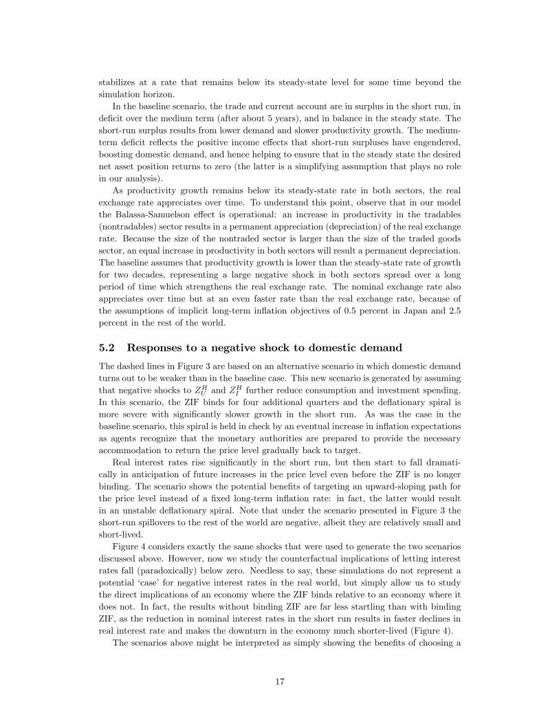
Under the same circumstances, could an appropriately designed PLPT rule do better?The answer is certainly yes. Figure 2 reconsiders the above experiment under two alternativeassumptions. First, the central bank now follows a PLPT rule where the annual slope ofthe price level path has been set to 2.5 percent. Second, the PLPT rule has been calibratedto avoid the undesirable consequences of an over-aggressive stance when the central bankattempts to close the price level gap too quickly: this simulation assumes a coe¢ cient of 0.5on the price level gap in the monetary reaction function.The higher slope for the price level path, relative to the case of a PLT rule, raises the

neutral policy rate by 2.5 percentage points and creates a signi�cant bu¤er that allowsrates to decline without hitting the ZIF. Note that the PLPT rule still requires a signi�cantincrease in interest rates in the short run. Also, as in�ation declines, the interest rate stillundershoots the neutral rate. But the contraction in real activity is now much less severethan it was in the previous case.With regard to the concern that PLPT rules might be less credible than pure IT rules,

it is important to emphasize that PLPT rules would only be used as a guideline for com-municating current and future policy actions, just like IT rules are currently used to helpconstruct and publish forecasts in countries that have adopted IT regimes. As is the case inthe latter regimes, the current stance of monetary policy is based on a plan for bringing in-�ation back to target gradually, and in a manner that is cognizant of the implications for thereal side of the economy. Under a PLPT rule the central bank�s forecast for in�ation wouldcontinue to represent an ideal intermediate target that is based on available information,and would need to be updated in a timely manner in response to new information.The only signi�cant di¤erence between a PLPT rule and a pure IT rule is that it would

generally take longer for the central bank�s forecast for in�ation to be equal its long-runtarget rate, as periods of above average in�ation would have to be o¤set by periods ofbelow-average in�ation to return the price level back towards its target path. It is di¢ cultto argue that such a rule would be less credible than simple in�ation-targeting rules, asan important prerequisite for a policy rule to be credible is that it has to be robust todi¤erent environments. We take as self-evident that pure in�ation-targeting rules, which bytheir very nature have to be abandoned when the ZIF binds, can never be as credible as anappropriately designed PLPT rule. Arguably, this point is even stronger in open economies.

18Similar considerations hold in the case of in�ation-targeting regimes. Critics have argued that IT couldresult in excessive variability in the real economy if central banks were committed to bringing in�ation backto target without concern for real objectives. In practice, central banks that have adopted IT regimes haveclearly recognized that, due to lags in the monetary transmission mechanism, it is not possible nor desirableto hit the target at each point in time.

15

As Svensson (2001) and others have pointed out, monetary authorities can always buildanti-de�ationary credibility by depreciating the exchange rate su¢ ciently to generate theexpectation of a higher price level in the future.

5 Some illustrative scenarios

In what follows, we consider a baseline and three illustrative scenarios to show the impli-cations of the ZIF in the presence of shocks that require easing monetary conditions. Weachieve this by simulating the economy�s responses to such shocks when the ZIF is binding,and by comparing them with similar responses when the ZIF is not binding.The �base case�aims to replicate a number of economic conditions in the recent past of

Japan, including low productivity growth and de�ation. This baseline scenario is assumed tobe the result of both low levels of domestic demand and a medium-term trend productivitygrowth that is below the long-term steady-state growth rate. More precisely, it is assumedthat over some period of time (two decades) ZHT and ZHN fall so that productivity growsa full 1 percentage point below the steady-state growth rate of 2 percent. Note that thissteady-state rate represents the growth rate of GDP in the long run as the analysis abstractsfrom population growth.The �rst scenario envisages a negative shock to domestic demand. The second and third

scenarios consider shocks to supply that raise the underlying rate of productivity growth inthe tradables sector and the nontradables sector, respectively. These two scenarios allow foran analysis of the implications of shocks to real exchange rates and the dynamics of macroadjustments along the lines of Balassa (1964) and Samuelson (1964).19 Before we proceed,it is worth emphasizing that our scenarios are purely illustrative and designed to illustratethe major mechanisms at work, as well as the key substantive issues involved with the ZIF.Needless to say, they are not intended to provide a plausible baseline forecast � nor tounderscore policy recommendations � for the Japanese economy.

5.1 An illustrative baseline with binding ZIF and temporary de�a-tion

The solid lines in Figure 3 illustrate our baseline scenario over a time horizon of ten years(40 quarters) for the following variables: GDP growth, the price level and its target path,CPI in�ation, nominal and real exchange rate, nominal and real interest rates, GDP growthin the rest of the world, the trade balance, and the current account balance. In the baselinescenario of Figure 3 the ZIF is assumed to be binding for the �rst seven quarters. In theshort run, there is de�ation � the combination of falling prices and low growth � but overthe medium term the economy recovers and in�ation expectations increase.As indicated earlier, recovery from the ZIF is ensured by assuming that monetary policy

is committed to following a rule where interest rates are adjusted to move the price levelgradually toward a �xed price level path that rises at the rate of 0.5 percent per annum.Expectations of higher in�ation � which result in a reduction of the real interest rate �combined with a weaker yen raise aggregate demand and boost actual in�ation. Growth

19The conditions for the Balassa-Samuelson e¤ect in the model depend on the combination of parame-ter values for the degree of home bias in consumption preferences, the elasticities of substitution betweendomestically-produced tradables and importables, as well as the elasticities of substitution between non-traded and traded goods.

16

stabilizes at a rate that remains below its steady-state level for some time beyond thesimulation horizon.In the baseline scenario, the trade and current account are in surplus in the short run, in

de�cit over the medium term (after about 5 years), and in balance in the steady state. Theshort-run surplus results from lower demand and slower productivity growth. The medium-term de�cit re�ects the positive income e¤ects that short-run surpluses have engendered,boosting domestic demand, and hence helping to ensure that in the steady state the desirednet asset position returns to zero (the latter is a simplifying assumption that plays no rolein our analysis).As productivity growth remains below its steady-state rate in both sectors, the real

exchange rate appreciates over time. To understand this point, observe that in our modelthe Balassa-Samuelson e¤ect is operational: an increase in productivity in the tradables(nontradables) sector results in a permanent appreciation (depreciation) of the real exchangerate. Because the size of the nontraded sector is larger than the size of the traded goodssector, an equal increase in productivity in both sectors will result a permanent depreciation.The baseline assumes that productivity growth is lower than the steady-state rate of growthfor two decades, representing a large negative shock in both sectors spread over a longperiod of time which strengthens the real exchange rate. The nominal exchange rate alsoappreciates over time but at an even faster rate than the real exchange rate, because ofthe assumptions of implicit long-term in�ation objectives of 0.5 percent in Japan and 2.5percent in the rest of the world.

5.2 Responses to a negative shock to domestic demand

The dashed lines in Figure 3 are based on an alternative scenario in which domestic demandturns out to be weaker than in the baseline case. This new scenario is generated by assumingthat negative shocks to ZHU and ZHI further reduce consumption and investment spending.In this scenario, the ZIF binds for four additional quarters and the de�ationary spiral ismore severe with signi�cantly slower growth in the short run. As was the case in thebaseline scenario, this spiral is held in check by an eventual increase in in�ation expectationsas agents recognize that the monetary authorities are prepared to provide the necessaryaccommodation to return the price level gradually back to target.Real interest rates rise signi�cantly in the short run, but then start to fall dramati-

cally in anticipation of future increases in the price level even before the ZIF is no longerbinding. The scenario shows the potential bene�ts of targeting an upward-sloping path forthe price level instead of a �xed long-term in�ation rate: in fact, the latter would resultin an unstable de�ationary spiral. Note that under the scenario presented in Figure 3 theshort-run spillovers to the rest of the world are negative, albeit they are relatively small andshort-lived.Figure 4 considers exactly the same shocks that were used to generate the two scenarios

discussed above. However, now we study the counterfactual implications of letting interestrates fall (paradoxically) below zero. Needless to say, these simulations do not represent apotential �case�for negative interest rates in the real world, but simply allow us to studythe direct implications of an economy where the ZIF binds relative to an economy where itdoes not. In fact, the results without binding ZIF are far less startling than with bindingZIF, as the reduction in nominal interest rates in the short run results in faster declines inreal interest rate and makes the downturn in the economy much shorter-lived (Figure 4).The scenarios above might be interpreted as simply showing the bene�ts of choosing a

17

high enough in�ation target that is explicitly designed to avoid the ZIF from binding. Theyactually go well beyond that, by demonstrating the equilibrating properties of monetarypolicy rules that embody PLPT. For example, in a fully-stochastic setting it is impossibleto rule out hitting the ZIF with pure in�ation-targeting rules, even if the in�ation targetis set as high as 2.0 percent � see Hunt and Laxton (2003). Since a monetary policy rulethat embodies PLPT will result in larger and more persistent declines in interest rates inresponse to de�ationary shocks than a pure in�ation-targeting rule, such a rule explicitlytakes the potential deleterious implications of the ZIF into account, and in practice it worksin the direction of reducing the probability of actually hitting the ZIF.Figure 4 also debunks a common �strawman� argument against PLPT, which is that

pursuing such rules in normal times would result in excessive variability in the businesscycle in the presence of signi�cant structural in�ation persistence. Such arguments areusually based on the assumption that the slope of the price-level target path is zero, or arebased on unrealistic assumptions about the degree of structural in�ation persistence in theeconomy. As can be seen in Figure 4, as long as PLPT rules are realistically designed �substantially, in order to bring the price level back to target very gradually � they shouldnot be expected to have harmful e¤ects on cyclical variability in normal times when thereis a small risk that the ZIF will become binding.20

To conclude this section, it is worthwhile to focus brie�y on the implications of openness.Figure 5 reconsiders the same scenarios as in Figure 3, but now the degree of openness inthe world economy is twice as large as the base case.21 Comparing Figure 5 with Figure 3suggests that a more open economy is less vulnerable to the problems associated with theZIF, in the sense that the same negative demand shock results in hitting the ZIF for a muchshorter period of time, and with less harmful e¤ects, relative to our base case. In the casewith more openness the negative demand shock causes the real exchange rate to depreciatein the short run, while it leads to an appreciation on impact under low openness. In bothcases de�ation results in very high real interest rates in the short run. With relatively lowopenness the real interest rate rise is persistent enough to strengthen the home currency inreal terms: real interest rates actually increase for one year after the shock. But in a regimeof high openness real interest rates are not expected to increase or even remain at a highlevel for a long time: in fact they start falling immediately after the shock, and the realexchange rate depreciates on impact. These results help explain why a model with a verylow degree of openness can become unstable, as a result of the change in the sign of the realexchange rate response.

5.3 Responses to positive supply shocks

The solid lines in Figure 6 reproduce the same baseline scenario discussed earlier in Figure3, but the dashed lines now illustrate an alternative scenario in which higher productivitygrowth in the tradables sector is added to the baseline scenario, possibly re�ecting the

20Most in�ation-targeting central banks usually choose a target signi�cantly above zero partly becauseof measurement problems, but also because of concerns that too low a target runs the risk of periodicallyhitting the ZIF in response to shocks. In fact, most in�ation-targeting countries typically choose a targetsuch as 2.0 percent or 2.5 percent, which is signi�cantly higher than what measurement bias alone wouldsuggest � see Batini, Kuttner and Laxton (2005). Using stochastic simulations, Hunt and Laxton (2003)argue that for countries with signi�cant nominal and real rigidities even an in�ation target as high as 2percent may be too low, because such targets combined with conventional monetary policy rules that ignoreprice-level considerations do not completely rule out hitting the ZIF.

21This is achieved by doubling the �HA , �HE , �

FA and �FE coe¢ cients relative to the baseline calibration.

18

outcome of structural transformations in the labor and product markets. Figure 7 simplyrepeats the analysis with the same shocks, but once again in this case interest rates areallowed to fall below zero. In these scenarios an increase in productivity in the tradablessector results in an appreciation in both the short run and the long run.As was the case for the negative demand shocks earlier, the appropriate policy response

is to reduce nominal interest rates relative to the baseline scenario whenever possible (eithernow if the ZIF is not binding, or in the future if it is binding). The rationale, however,is di¤erent. In the earlier scenario of negative demand shocks, a commitment to easingmonetary conditions prevented demand from falling further and ensured the injection ofsu¢ cient nominal stimulus to stop an ongoing de�ationary spiral. In the scenarios of Figures6 and 7, instead, the positive supply shock actually raises output. However, if the economystarts at the ZIF, supply shocks can extend the period of time over which the ZIF remainsbinding. In our particular example it extends the period of time the ZIF binds by 2 quarters.Prima facie comparison of Figures 6 and 7 might suggest that there are only minor

complications associated with hitting the ZIF for a longer period of time, as there are smalldi¤erences between the pro�les for real activity and in�ation when the ZIF binds and whenit does not. Unfortunately, this type of inference derived from deterministic simulationscenarios underestimates the potential complications of supply shocks in the real world, asit implicitly assumes that no further demand or supply shocks would occur in the future.There could be instances where an economy, which is expected to remain for some time atthe ZIF as growth-enhancing structural reforms proceed, were to be hit by a new series ofnegative aggregate demand shocks. In this case the e¤ects of these new shocks would beampli�ed because they would be �layered�upon a scenario in which the ZIF was alreadybinding.To analyze the implications of supply shocks that are concentrated in the nontradables

sector, we repeat the above analysis under the assumption that the productivity growthshock is concentrated in the N sector of our model � see Figures 8 and 9. A similar storyemerges. The appropriate policy response is to reduce interest rates when it is possible(either now or in the future), and in the case where the ZIF is binding it binds for longer.However, in this case because the shock is concentrated in the nontradables sector it resultsin a depreciation of the real exchange rate and stronger growth in the short run. As aconsequence, when the ZIF is not binding interest rates decline in the short run, but then riseafter 2 years to contain the ensuing in�ationary pressures stemming from the depreciationof the currency. In this case, the ZIF binds for only one additional quarter relative to thebaseline, compared with two quarters when the productivity shock was concentrated in thetradables sector.

5.4 Raising the in�ation target to 2.5 percent

The simulations reported earlier highlight the potential bene�ts of moving the economyaway from the ZIF as quickly as possible, once the economy hits it.22 Figures 10 and 11illustrate the implications of increasing the slope of the price level target path in the baselinefrom 0.5 percent to 2.5 percent, per annum.Figure 10 considers the case where the ZIF is binding initially. In this case, if such a

policy were perceived to be credible, it would result in an increase of in�ation expectations

22A growing empirical literature shows that central banks in in�ation-targeting countries have had sig-ni�cant success in anchoring long-term in�ation expectations to their targets � see in particular Levin,Natalucci and Piger (2004), Batini, Kuttner and Laxton (2005), Gürkaynak, Sack, and Swanson (2005).

19

in the short run, and the period of time over which the ZIF is expected to be binding wouldshrink. In this particular example, the home country economy is at the ZIF for 4 quartersinstead of the 7 quarters in the baseline scenario. Figure 11 reports the case where theZIF is not binding. Interest rates decline in the short run, providing the reduction in realinterest rates needed to stimulate aggregate demand. This increases in�ation gradually toits new permanently higher level.It is sometimes argued that, in practice, it may be di¢ cult to implement such a policy

when the ZIF is binding, because the lower real interest rates which are required to stimulateaggregate demand in the short run work entirely through an expectational channel, and byde�nition cannot be backed up in terms of a reduction in nominal short-term interest rates.However, this argument assumes that the central bank will not take other measures to ensurethe credibility of the policy strategy. This assumption seems highly unrealistic. Eggertssonand Woodford (2003, 2004) highlight that both monetary and �scal authorities face a largemenu of actions, including the purchase of government securities and real estate assets, toguarantee their commitment to achieving higher price levels in the future. And, as alreadymentioned, in the context of an open economy it is always possible to engineer su¢ cientexchange rate depreciation to generate credible expectations of a higher price level in thefuture.

6 Conclusion

Using a two-country simulation model calibrated to the Japanese economy, this paper hascarried out a scenario analysis to illustrate possible di¢ culties in dealing with both demandand supply shocks when the ZIF is binding. The key results concerning the implicationsof openness on the e¤ectiveness of monetary rules in a de�ationary environment have beenhighlighted at length and need not be rehashed here. Instead, we conclude by commentingbrie�y on a few directions for further research.The basic insight of the large body of literature on policy rules is that it is not essential

to derive optimal rules based on speci�c models or views about the economy, but ratherto search for rules that are robust across di¤erent environments and circumstances. Thearguments in the paper, which are based on illustrative scenarios, suggest that PLPT rulesshould be expected to have signi�cant advantages over either pure IT rules or pure PLTrules (to some extent, PLPT rules combine the best from both IT and PLT approaches).The obvious extension would be to evaluate alternative rules in a fully stochastic environ-ment and, in fact, doing so would likely strengthen the bene�ts of PLPT rules over theiralternatives.For example, the analysis has ignored the permanent welfare consequences and dead-

weight losses that would be associated with rules that periodically allow for the occurrenceof long de�ationary spirals. Also, relative to IT rules, our analysis above has abstractedfrom the possible welfare bene�ts that PLPT rules could generate, stemming from loweruncertainty about the future price level. While the e¤ects of uncertainty about price levelmovements has perhaps been overlooked in this literature, it may become a key issue overtime as the policy debate focuses on the demographic consequences of population aging.

20

References

[1] Balassa B., 1964, "The Purchasing Power Doctrine: A Reappraisal," Journal of PoliticalEconomy, Vol. 72, pp. 585-596.

[2] Batini, N., K. Kuttner, and D. Laxton, 2005, �Does In�ation Targeting Work in Emerg-ing Markets?�, World Economic Outlook, Chapter IV, 161�86.

[3] Batini, N., P. N�Diaye, and A. Rebucci, "The Domestic and Global Impact of Japan�sPolicies for Growth," IMF Working Paper No. 05/209.

[4] Bayoumi, T., D. Laxton, and P. Pesenti, 2004, "Bene�ts and Spillovers of GreaterCompetition in Europe: A Macroeconomic Assessment", NBER Working Paper No.10416.

[5] Callen, T., and J. D. Ostry, 2003, Japan�s Lost Decade, Policies for Economic Revival,Washington: International Monetary Fund, pp.179-205.

[6] Christiano L., M. Eichenbaum, C. Evans, 1999, "Monetary Policy Shocks: What HaveWe Learned and To What End?," in Taylor,J., Woodford, M., eds., Handbook of Macro-economics, Vol. 1A, Amsterdam: North Holland, pp. 65-148.

[7] Eggertsson, G., and M. Woodford, 2003, "Optimal Monetary Policy in a LiquidityTrap," International Workshop on Overcoming De�ation and Revitalizing the JapaneseEconomy (August)�

[8] Eggertsson, G., and M. Woodford, 2004, "Optimal Monetary and Fiscal Policy in aLiquidity Trap," NBER International Seminar on Macroeconomics (July).

[9] Faruqee, H., D. Laxton, D. Muir and P. Pesenti, 2006, "Smooth Landing or Crash?Model-based Scenarios of Global Current Account Rebalancing," forthcoming in R.Clarida (ed.), G7 Current Account Imbalances: Sustainability and Adjustment, NBERconference volume, Chicago, IL: University of Chicago Press.

[10] Greenwood, J., Z. Hercowitz and G.W. Hu¤man, 1988, "Investment, Capacity Uti-lization, and the Real Business Cycle," American Economic Review, Vol. 78(3), pp.402-17.

[11] Gürkaynak, R., B. Sack, and E. Swanson, 2005, �The Sensitivity of Long-Term InterestRates to Economic News: Evidence and Implications for Macroeconomic Models�,American Economic Review, Vol. 95, 425�36.

[12] Hayami, M., 2001, "Opening Speech", Monetary and Economic Studies, Vol.19(S-1),pp. 9-12

[13] Hayashi, F., and E.C. Prescott, "The 1990�s in Japan: A Lost Decade," The FinalInternational Forum of the Collaboration Projects.

[14] Hunt, B., and D. Laxton, 2001, "The Zero Interest Rate Floor (ZIF) and Its Implica-tions for Monetary Policy in Japan," IMF Working Paper 01/186.

[15] Hunt, B. and D. Laxton, 2003, "The Zero-Interest-Rate Floor and Its Implications forMonetary Policy in Japan," in Tim Callen and Jonathan D. Ostry, eds., Japan�s LostDecade, Policies for Economic Revival, Washington: International Monetary Fund,pp.179-205.

21

[16] Laxton, D., P. Isard, H. Faruqee, E. Prasad, and B. Turtelboom, 1998, MULTIMODMark III: The Core Steady-State Models, IMF Occasional Paper No. 164.

[17] Levin, A., F. Natalucci, and J. Piger, (2004), �The Macroeconomic E¤ects of In�ationTargeting�, Federal Reserve Bank of St. Louis Review, Vol. 86(4), pp. 51�80.

[18] McCallum, B. T., 2000, "Theoretical Analysis Regarding a Zero Lower Bound on Nom-inal Interest Rates," Journal of Money, Credit and Banking, Vol. 32(4), pp. 870-904,(November).

[19] McCallum, B. T., 2001, "In�ation Targeting and the Liquidity Trap," NBER WorkingPaper No. 8225.

[20] Samuelson, P. , 1964, "Theoretical Notes on Trade Problems", Review of Economicsand Statistics, Vol. 46, pp. 145-154.

[21] Svensson, L.E.O., 2001, "The Zero Bound in an Open Economy: A Foolproof Way ofEscaping From a Liquidity Trap,"Monetary and Economic Studies, Vol. 19 (February),pp.277-312.

[22] Taylor, J.B., 1993, "Discretion Versus Policy Rules in Practice," Carnegie-RochesterConference Series on Public Policy, Vol. 39 (December) pp. 195-214.

22

Table 1: Steady-State National Accounts in the Baseline Scenario

(Percentage Shares of GDP)

H F

Private Consumption CSS=GDPSS 56.97 64.86Forward-looking consumers CFL;SS=GDPSS 50.18 56.12Liquidity-constrained consumers CLC;SS=GDPSS 6.80 8.74Private Investment pE;SSISS=GDPSS 23.53 17.14Public Expenditure GSS=GDPSS 19.50 18.00Trade balance TBALSS=GDPSS 0.00 0.00Imports IMSS=GDPSS 11.03 1.45Consumption Goods pMA;SSMA;SS=GDPSS 7.62 0.72Investment Goods pME;SSME;SS=GDPSS 3.42 0.73Net Foreign Assets bF;RAT;SS 0.00 0.00Share of World GDP (percent) s 11.59 88.41

Table 2: Households and Firms Parameters

H F

Share of liquidity constrained consumers sLC 0.40 0.40Annualized rate of time preference 100 �

���4SS � 1

�1.43 2.59

Depreciation rate � 0.02 0.02Intertemporal elasticity of substitution 1=� 5.00 5.00Habit persistence in consumption bc 0.91 0.91Inverse of the Frisch elasticity of labor & 2.50 2.50Habit persistence in labor b` 0.75 0.75Tradable Intermediate GoodsSubstitution between factors of production �T 0.75 0.75Weight of capital �KT 0.73 0.57Nontradable Intermediate GoodsSubstitution between factors of production �N 0.75 0.75Weight of capital �KN .70 0.56Final Consumption GoodsSubstitution between domestic and imported goods �A 2.50 2.50Weight of domestic goods �A 0.59 0.97Substitution between domestic tradables and nontradables "A 0.50 0.50Weight of tradable goods A 0.36 0.34Final Investment GoodsSubstitution between domestic and imported goods �E 2.50 2.50Weight of domestic goods �E 0.81 0.96Substitution between domestic tradables and nontradables "E 0.50 0.50Bias towards tradable goods E 0.77 0.75

23

Table 3: Price and Wage Markups

H F

TradablesMarkup �T =(�T � 1) 1.26 1.18NontradablesMarkup �N=(�N � 1) 1.29 1.23WagesMarkup =( � 1) 1.20 1.20

Table 4: Nominal and Real Rigidities

H F

Real RigiditiesCapital accumulation �I1 1.00 1.00Investment changes �I2 78.00 78.00Imports of consumption goods �MA 0.95 0.95Imports of investment goods �ME 0.95 0.95Nominal RigiditiesWages of liquidity-constrained consumers �WLC 400 400Wages of forward-looking consumers �WFL 400 400Prices of domestic tradables �PQ 400 400Prices of nontradables �PN 400 400Prices of imports �PM 3200 3200

Table 5: Base-Case Monetary Policy Reaction Function ParametersH F

In�ation gap !� 2.0 2.0Price Level gap !P 0.5 0.0

24

Figure 1: Price Level is Initially 5 Percent Higher Than Target With a Zero Slope in theTarget Path

­4

­2

0

2

4

6

­4

­2

0

2

4

6

0 4 8 12 16 20 24 28 32 36 40

GDP Growth(In percent; year­on­year)

98

100

102

104

106

98

100

102

104

106

0 4 8 12 16 20 24 28 32 36 40

Price Level and Target(In percent)

­4

­3

­2

­1

0

1

­4

­3

­2

­1

0

1

0 4 8 12 16 20 24 28 32 36 40

Inflation(In percent; year­on­year)

0

5

10

15

0

5

10

15

0 4 8 12 16 20 24 28 32 36 40

Nominal Interest Rates(In percent)

25

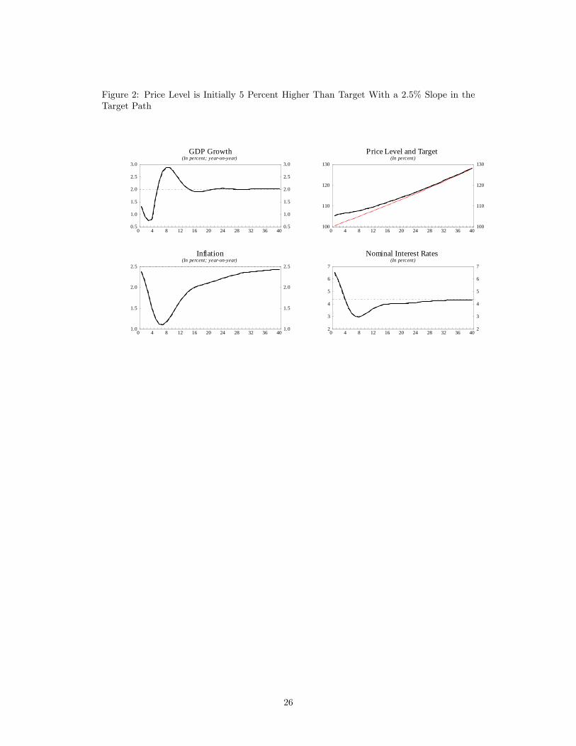
Figure 2: Price Level is Initially 5 Percent Higher Than Target With a 2.5% Slope in theTarget Path

0.5

1.0

1.5

2.0

2.5

3.0

0.5

1.0

1.5

2.0

2.5

3.0

0 4 8 12 16 20 24 28 32 36 40

GDP Growth(In percent; year­on­year)

100

110

120

130

100

110

120

130

0 4 8 12 16 20 24 28 32 36 40

Price Level and Target(In percent)

1.0

1.5

2.0

2.5

1.0

1.5

2.0

2.5

0 4 8 12 16 20 24 28 32 36 40

Inflation(In percent; year­on­year)

2

3

4

5

6

7

2

3

4

5

6

7

0 4 8 12 16 20 24 28 32 36 40

Nominal Interest Rates(In percent)

26

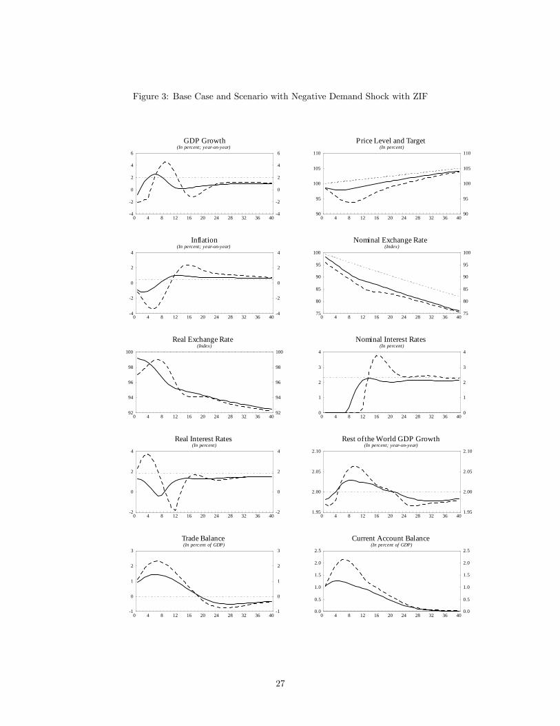
Figure 3: Base Case and Scenario with Negative Demand Shock with ZIF

­4

­2

0

2

4

6

­4

­2

0

2

4

6

0 4 8 12 16 20 24 28 32 36 40

GDP Growth(In percent; year­on­year)

90

95

100

105

110

90

95

100

105

110

0 4 8 12 16 20 24 28 32 36 40

Price Level and Target(In percent)

­4

­2

0

2

4

­4

­2

0

2

4

0 4 8 12 16 20 24 28 32 36 40

Inflation(In percent; year­on­year)

75

80

85

90

95

100

75

80

85

90

95

100

0 4 8 12 16 20 24 28 32 36 40

Nominal Exchange Rate(Index)

92

94

96

98

100

92

94

96

98

100

0 4 8 12 16 20 24 28 32 36 40

Real Exchange Rate(Index)

0

1

2

3

4

0

1

2

3

4

0 4 8 12 16 20 24 28 32 36 40

Nominal Interest Rates(In percent)

­2

0

2

4

­2

0

2

4

0 4 8 12 16 20 24 28 32 36 40

Real Interest Rates(In percent)

1.95

2.00

2.05

2.10

1.95

2.00

2.05

2.10

0 4 8 12 16 20 24 28 32 36 40

Rest of the World GDP Growth(In percent; year­on­year)

­1

0

1

2

3

­1

0

1

2

3

0 4 8 12 16 20 24 28 32 36 40

Trade Balance(In percent of GDP)

0.0

0.5

1.0

1.5

2.0

2.5

0.0

0.5

1.0

1.5

2.0

2.5

0 4 8 12 16 20 24 28 32 36 40

Current Account Balance(In percent of GDP)

27

Figure 4: Base Case and Scenario with Negative Demand Shock without ZIF

­1

0

1

2

3

­1

0

1

2

3

0 4 8 12 16 20 24 28 32 36 40

GDP Growth(In percent; year­on­year)

98

100

102

104

106

98

100

102

104

106

0 4 8 12 16 20 24 28 32 36 40

Price Level and Target(In percent)

­1.0

­0.5

0.0

0.5

1.0

­1.0

­0.5

0.0

0.5

1.0

0 4 8 12 16 20 24 28 32 36 40

Inflation(In percent; year­on­year)

70

80

90

100

70

80

90

100

0 4 8 12 16 20 24 28 32 36 40

Nominal Exchange Rate(Index)

90

95

100

105

90

95

100

105

0 4 8 12 16 20 24 28 32 36 40

Real Exchange Rate(Index)

­2

­1

0

1

2

3

­2

­1

0

1

2

3

0 4 8 12 16 20 24 28 32 36 40

Nominal Interest Rates(In percent)

­1

0

1

2

­1

0

1

2

0 4 8 12 16 20 24 28 32 36 40

Real Interest Rates(In percent)

1.96

1.98

2.00

2.02

2.04

1.96

1.98

2.00

2.02

2.04

0 4 8 12 16 20 24 28 32 36 40

Rest of the World GDP Growth(In percent; year­on­year)

­1

0

1

2

­1

0

1

2

0 4 8 12 16 20 24 28 32 36 40

Trade Balance(In percent of GDP)

0.0

0.5

1.0

1.5

0.0

0.5

1.0

1.5

0 4 8 12 16 20 24 28 32 36 40

Current Account Balance(In percent of GDP)

28

Figure 5: Base Case and Scenario with Negative Demand Shock with ZIF and DoubleOpenness

­1

0

1

2

3

­1

0

1

2

3

0 4 8 12 16 20 24 28 32 36 40

GDP Growth(In percent; year­on­year)

98

100

102

104

106

98

100

102

104

106

0 4 8 12 16 20 24 28 32 36 40

Price Level and Target(In percent)

­1.0

­0.5

0.0

0.5

1.0

­1.0

­0.5

0.0

0.5

1.0

0 4 8 12 16 20 24 28 32 36 40

Inflation(In percent; year­on­year)

75

80

85

90

95

100

75

80

85

90

95

100

0 4 8 12 16 20 24 28 32 36 40

Nominal Exchange Rate(Index)

92

94

96

98

100

92

94

96

98

100

0 4 8 12 16 20 24 28 32 36 40

Real Exchange Rate(Index)

0.0

0.5

1.0

1.5

2.0

2.5

0.0

0.5

1.0

1.5

2.0

2.5

0 4 8 12 16 20 24 28 32 36 40

Nominal Interest Rates(In percent)

­0.5

0.0

0.5

1.0

1.5

2.0

­0.5

0.0

0.5

1.0

1.5

2.0

0 4 8 12 16 20 24 28 32 36 40

Real Interest Rates(In percent)

1.90

1.95

2.00

2.05

2.10

1.90

1.95

2.00

2.05

2.10

0 4 8 12 16 20 24 28 32 36 40

Rest of the World GDP Growth(In percent; year­on­year)

­2

­1

0

1

2

3

­2

­1

0

1

2

3

0 4 8 12 16 20 24 28 32 36 40

Trade Balance(In percent of GDP)

­1

0

1

2

3

­1

0

1

2

3

0 4 8 12 16 20 24 28 32 36 40

Current Account Balance(In percent of GDP)

29

Figure 6: Base Case and Scenario with Productivity Growth Shock in Tradables Sector withZIF

­1

0

1

2

3

4

­1

0

1

2

3

4

0 4 8 12 16 20 24 28 32 36 40

GDP Growth(In percent; year­on­year)

96

98

100

102

104

106

96

98

100

102

104

106

0 4 8 12 16 20 24 28 32 36 40

Price Level and Target(In percent)

­2

­1

0

1

2

­2

­1

0

1

2

0 4 8 12 16 20 24 28 32 36 40

Inflation(In percent; year­on­year)

70

80

90

100

110

70

80

90

100

110

0 4 8 12 16 20 24 28 32 36 40

Nominal Exchange Rate(Index)

85

90

95

100

85

90

95

100

0 4 8 12 16 20 24 28 32 36 40

Real Exchange Rate(Index)

0.0

0.5

1.0

1.5

2.0

2.5

0.0

0.5

1.0

1.5

2.0

2.5

0 4 8 12 16 20 24 28 32 36 40

Nominal Interest Rates(In percent)

­1

0

1

2

­1

0

1

2

0 4 8 12 16 20 24 28 32 36 40

Real Interest Rates(In percent)

1.96

1.98

2.00

2.02

2.04

2.06

1.96

1.98

2.00

2.02

2.04

2.06

0 4 8 12 16 20 24 28 32 36 40

Rest of the World GDP Growth(In percent; year­on­year)

­2

­1

0

1

2

­2

­1

0

1

2

0 4 8 12 16 20 24 28 32 36 40

Trade Balance(In percent of GDP)

­1.0

­0.5

0.0

0.5

1.0

1.5

­1.0

­0.5

0.0

0.5

1.0

1.5

0 4 8 12 16 20 24 28 32 36 40

Current Account Balance(In percent of GDP)

30

Figure 7: Base Case and Scenario with Productivity Growth Shock in Tradables Sectorwithout ZIF

­1

0

1

2

3

­1

0

1

2

3

0 4 8 12 16 20 24 28 32 36 40

GDP Growth(In percent; year­on­year)

98

100

102

104

106

98

100

102

104

106

0 4 8 12 16 20 24 28 32 36 40

Price Level and Target(In percent)

­1.0

­0.5

0.0

0.5

1.0

­1.0

­0.5

0.0

0.5

1.0

0 4 8 12 16 20 24 28 32 36 40

Inflation(In percent; year­on­year)

70

80

90

100

110

70

80

90

100

110

0 4 8 12 16 20 24 28 32 36 40

Nominal Exchange Rate(Index)

85

90

95

100

85

90

95

100

0 4 8 12 16 20 24 28 32 36 40

Real Exchange Rate(Index)

­1

0

1

2

3

­1

0

1

2

3

0 4 8 12 16 20 24 28 32 36 40

Nominal Interest Rates(In percent)

­0.5

0.0

0.5

1.0

1.5

2.0

­0.5

0.0

0.5

1.0

1.5

2.0

0 4 8 12 16 20 24 28 32 36 40

Real Interest Rates(In percent)

1.96

1.98

2.00

2.02

2.04

1.96

1.98

2.00

2.02

2.04

0 4 8 12 16 20 24 28 32 36 40

Rest of the World GDP Growth(In percent; year­on­year)

­2

­1

0

1

2

­2

­1

0

1

2

0 4 8 12 16 20 24 28 32 36 40

Trade Balance(In percent of GDP)

­1.0

­0.5

0.0

0.5

1.0

1.5

­1.0

­0.5

0.0

0.5

1.0

1.5

0 4 8 12 16 20 24 28 32 36 40

Current Account Balance(In percent of GDP)

31

Figure 8: Base Case and Scenario with Productivity Growth Shock in Non-Tradables Sectorwith ZIF

­2

0

2

4

6

­2

0

2

4

6

0 4 8 12 16 20 24 28 32 36 40

GDP Growth(In percent; year­on­year)

96

98

100

102

104

106

96

98

100

102

104

106

0 4 8 12 16 20 24 28 32 36 40

Price Level and Target(In percent)

­2

­1

0

1

2

­2

­1

0

1

2

0 4 8 12 16 20 24 28 32 36 40

Inflation(In percent; year­on­year)

70

80

90

100

110

70

80

90

100

110

0 4 8 12 16 20 24 28 32 36 40

Nominal Exchange Rate(Index)

90

95

100

105

90

95

100

105

0 4 8 12 16 20 24 28 32 36 40

Real Exchange Rate(Index)

0

1

2

3

4

0

1

2

3

4

0 4 8 12 16 20 24 28 32 36 40

Nominal Interest Rates(In percent)

­1

0

1

2

­1

0

1

2

0 4 8 12 16 20 24 28 32 36 40

Real Interest Rates(In percent)

1.96

1.98

2.00

2.02

2.04

1.96

1.98

2.00

2.02

2.04

0 4 8 12 16 20 24 28 32 36 40

Rest of the World GDP Growth(In percent; year­on­year)

­1

0

1

2

3

­1

0

1

2

3

0 4 8 12 16 20 24 28 32 36 40

Trade Balance(In percent of GDP)

0.0

0.5

1.0

1.5

2.0

0.0

0.5

1.0

1.5

2.0

0 4 8 12 16 20 24 28 32 36 40

Current Account Balance(In percent of GDP)

32

Figure 9: Base Case and Scenario with Productivity Growth Shock in Non-Tradables Sectorwithout ZIF

­1

0

1

2

3

4

­1

0

1

2

3

4

0 4 8 12 16 20 24 28 32 36 40

GDP Growth(In percent; year­on­year)

98

100

102

104

106

98

100

102

104

106

0 4 8 12 16 20 24 28 32 36 40

Price Level and Target(In percent)

­1.0

­0.5

0.0

0.5

1.0

1.5

­1.0

­0.5

0.0

0.5

1.0

1.5

0 4 8 12 16 20 24 28 32 36 40

Inflation(In percent; year­on­year)

70

80

90

100

110

70

80

90

100

110

0 4 8 12 16 20 24 28 32 36 40

Nominal Exchange Rate(Index)

90

95

100

105

90

95

100

105

0 4 8 12 16 20 24 28 32 36 40

Real Exchange Rate(Index)

­1

0

1

2

3

­1

0

1

2

3

0 4 8 12 16 20 24 28 32 36 40

Nominal Interest Rates(In percent)

­0.5

0.0

0.5

1.0

1.5

2.0

­0.5

0.0

0.5

1.0

1.5

2.0

0 4 8 12 16 20 24 28 32 36 40

Real Interest Rates(In percent)

1.96

1.98

2.00

2.02

2.04

1.96

1.98

2.00

2.02

2.04

0 4 8 12 16 20 24 28 32 36 40

Rest of the World GDP Growth(In percent; year­on­year)

­1

0

1

2

3

­1

0

1

2

3

0 4 8 12 16 20 24 28 32 36 40

Trade Balance(In percent of GDP)

0.0

0.5

1.0

1.5

2.0

0.0

0.5

1.0

1.5

2.0

0 4 8 12 16 20 24 28 32 36 40

Current Account Balance(In percent of GDP)

33

Figure 10: Base Case and New Scenario with an Annual 2.5% Slope in the Price LevelTarget Path with ZIF

­1

0

1

2

3

4

­1

0

1

2

3

4

0 4 8 12 16 20 24 28 32 36 40

GDP Growth(In percent; year­on­year)

90

100

110

120

130

90

100

110

120

130

0 4 8 12 16 20 24 28 32 36 40

Price Level and Target(In percent)

­2

0

2

4

­2

0

2

4

0 4 8 12 16 20 24 28 32 36 40

Inflation(In percent; year­on­year)

70

80

90

100

110

70

80

90

100

110

0 4 8 12 16 20 24 28 32 36 40

Nominal Exchange Rate(Index)

92

94

96

98

100

102

92

94

96

98

100

102

0 4 8 12 16 20 24 28 32 36 40

Real Exchange Rate(Index)

0

1

2

3

4

5

0

1

2

3

4

5

0 4 8 12 16 20 24 28 32 36 40

Nominal Interest Rates(In percent)

­2

­1

0

1

2

­2

­1

0

1

2

0 4 8 12 16 20 24 28 32 36 40

Real Interest Rates(In percent)

1.96

1.98

2.00

2.02

2.04

1.96

1.98

2.00

2.02

2.04

0 4 8 12 16 20 24 28 32 36 40

Rest of the World GDP Growth(In percent; year­on­year)

­1.0

­0.5

0.0

0.5

1.0

1.5

­1.0

­0.5

0.0

0.5

1.0

1.5

0 4 8 12 16 20 24 28 32 36 40

Trade Balance(In percent of GDP)

0.0

0.5

1.0

1.5

0.0

0.5

1.0

1.5

0 4 8 12 16 20 24 28 32 36 40

Current Account Balance(In percent of GDP)

34

Figure 11: Base Case and New Scenario with an Annual 2.5% Slope in the Price LevelTarget Path without ZIF

­1

0

1

2

3

4

­1

0

1

2

3

4

0 4 8 12 16 20 24 28 32 36 40

GDP Growth(In percent; year­on­year)

90

100

110

120

130

90

100

110

120

130

0 4 8 12 16 20 24 28 32 36 40

Price Level and Target(In percent)

­1

0

1

2

3

­1

0

1

2

3

0 4 8 12 16 20 24 28 32 36 40

Inflation(In percent; year­on­year)

70

80

90

100

110

70

80

90

100

110

0 4 8 12 16 20 24 28 32 36 40

Nominal Exchange Rate(Index)

90

95

100

105

90

95

100

105

0 4 8 12 16 20 24 28 32 36 40

Real Exchange Rate(Index)

­2

0

2

4

6

­2

0

2

4

6

0 4 8 12 16 20 24 28 32 36 40

Nominal Interest Rates(In percent)

­3

­2

­1

0

1

2

­3

­2

­1

0

1

2

0 4 8 12 16 20 24 28 32 36 40

Real Interest Rates(In percent)

1.96

1.98

2.00

2.02

2.04

1.96

1.98

2.00

2.02

2.04

0 4 8 12 16 20 24 28 32 36 40

Rest of the World GDP Growth(In percent; year­on­year)

­1.0

­0.5

0.0

0.5

1.0

1.5

­1.0

­0.5

0.0

0.5

1.0

1.5

0 4 8 12 16 20 24 28 32 36 40

Trade Balance(In percent of GDP)

0.0

0.5

1.0

1.5

0.0

0.5

1.0

1.5

0 4 8 12 16 20 24 28 32 36 40

Current Account Balance(In percent of GDP)

35