deepjdot: deep joint distribution optimal transport for ... · deepjdot: deep joint distribution...

DeepJDOT: Deep Joint Distribution OptimalTransport for Unsupervised Domain Adaptation

Bharath Bhushan Damodaran1? , Benjamin Kellenberger2∗, Remi Flamary3,Devis Tuia2, Nicolas Courty1

1 Universite de Bretagne Sud, IRISA, UMR 6074, CNRS, France2 Wageningen University, the Netherlands

3 Universite Cote d’Azur, OCA, UMR 7293, CNRS, Laboratoire Lagrange, France{[email protected], [email protected]}

Abstract. In computer vision, one is often confronted with problemsof domain shifts, which occur when one applies a classifier trained on asource dataset to target data sharing similar characteristics (e.g. sameclasses), but also different latent data structures (e.g. different acquisitionconditions). In such a situation, the model will perform poorly on the newdata, since the classifier is specialized to recognize visual cues specific tothe source domain. In this work we explore a solution, named DeepJDOT,to tackle this problem: through a measure of discrepancy on joint deeprepresentations/labels based on optimal transport, we not only learnnew data representations aligned between the source and target domain,but also simultaneously preserve the discriminative information used bythe classifier. We applied DeepJDOT to a series of visual recognitiontasks, where it compares favorably against state-of-the-art deep domainadaptation methods.

Keywords: Deep Domain Adaptation, Optimal Transport

1 Introduction

The ability to generalize across datasets is one of the holy grails of computervision. Designing models that can perform well on datasets sharing similar char-acteristics such as classes, but also presenting different underlying data struc-tures (for instance different backgrounds, colorspaces, or acquired with differentdevices) is key in applications where labels are scarce or expensive to obtain.However, traditional learning machines struggle in performing well out of thedatasets (or domains) they have been trained with. This is because models gen-erally assume that both training (or source) and test (or target) data are issuedfrom the same generating process. In vision problems, factors such as objectsposition, illumination, number of channels or seasonality break this assumptionand call for adaptation strategies able to compensate for such shifts, or domainadaptation strategies [1].

? authors contributed equally

arX

iv:1

803.

1008

1v3

[cs

.CV

] 5

Sep

201

8

2 B.B. Damodaran et al.

In a first rough subdivision, domain adaptation strategies can be separatedinto unsupervised and semi-supervised domain adaptation: the former assumesthat no labels are available in the target domain, while the latter assumes thepresence of a few labeled instances in the target domain that can be used asreference points for the adaptation. In this paper, we propose a contribution forthe former, more challenging case. Let xs ∈ XS be the source domain exam-ples with the associated labels ys ∈ YS . Similarly, let xt ∈ XT be the targetdomain images, but with unknown labels. The goal of the unsupervised domainadaptation is to learn the classifier f in the target domain by leveraging theinformation from the source domain. To this end, we have access to a sourcedomain dataset {xsi , ys}i=1,...,ns and a target domain dataset {xti}i=1,...,nt withonly observations and no labels.

Early unsupervised domain adaptation research tackled the problem as theone of finding a common representation between the domains, or a latent space,where a single classifier can be used independently from the datapoint’s origin [2,3]. In [4], the authors propose to use discrete optimal transport to match theshifted marginal distributions of the two domains under constraints of classregularity in the source. In [5] a similar logic is used, but the joint distributionsare aligned directly using a coupling accounting for the marginals and the class-conditional distributions shift jointly. However, the method has two drawbacks,for which we propose solutions in this paper: 1) first, the JDOT method in[5] scales poorly, as it must solve a n1 × n2 coupling, where n1 and n2 are thesamples to be aligned; 2) secondly, the optimal transport coupling γ is computedbetween the input spaces (and using a `2 distance), which is a poor representationto be aligned, since we are interested in matching more semantic representationssupposed to ease the work of the classifier using them to take decisions.

We solve the two problems above by a strategy based on deep learning. Onthe one hand, using deep learning algorithms for domain adaptation has foundan increasing interest and has shown impressive results in recent computer vi-sion literature [6–9]. On the other hand (and more importantly), a ConvolutionalNeural Network (CNN) offers the characteristics needed to solve our two prob-lems: 1) by gradually adapting the optimal transport coupling along the CNNtraining, we obtain a scalable solution, an approximated and stochastic versionof JDOT; 2) by learning the coupling in a deep layer of the CNN, we alignthe representation the classifier is using to take its decision, which is a moresemantic representation of the classes. In summary, we learn jointly the embed-ding between the two domains and the classifier in a single CNN framework. Weuse a domain adaptation-tailored loss function based on optimal transport andtherefore call our proposition Deep Joint Distribution Optimal Transportation(DeepJDOT).

We test DeepJDOT on a series of visual domain adaptation tasks and com-pare favorably against several recent state of the art competitors.

DeepJDOT 3

2 Related works

Unsupervised domain adaptation. Unsupervised domain adaptation studies thesituation where the source domain carries labeled instances, while the targetdomain is unlabeled, yet accessible during training [10]. Earlier approaches con-sider projections aligning data spaces to each other [2, 11, 12], thus trying to ex-ploit shift-invariant information to match the domains in their original (input)space. Later works extended such logic to deep learning, typically by weightsharing [6]/reconstruction [13], by adding Maximum Mean Discrepancy (MMD)and association-based losses between source and target layers [14–16]. Other ma-jor developments focus on the inclusion of adversarial loss functions pushing theCNN to be unable to discriminate whether a sample comes from the source orthe target domain [7, 8, 17]. Finally, the most recent works extend this adver-sarial logic to the use of GANs [18, 19], for example using two GAN moduleswith shared weights [9], forcing image to image architectures to have similaractivation distributions [20] or simply fooling a GAN’s discriminator discerningbetween domains [21]. These adversarial image generation based methods [18–20] use a class-conditioning or cycle consistency term to learn the discriminativeembedding, such that semantically similar images in both domains are projectedcloseby in the embedding space. Our proposed DeepJDOT uses the concept ofa shared embedding for both domains [17] and is built on a similar logic asthe MMD-based methods, yet adding a clear discriminative component to thealignment: the proposed DeepJDOT associates representation and discrimina-tive learning, since the optimal transport coupling ensures that distributions arematched, while i) the JDOT class loss performs source label propagation to thetarget samples and ii) the fact of learning the coupling in deep layers of theCNN ensures discrimination power.

Optimal transport in domain adaptation. Optimal transport [22–24] has beenused in domain adaptation to learn the transformation between domains [4, 25,26], with associated theoretical guarantees [27]. In those works, the coupling γ isused to transport (i.e. transform) the source data samples through an estimatedmapping called barycentric mapping. Then, a new classifier is trained on thetransported source data representation. But those different methods can onlyaddress problems of small to medium sizes because they rely on the exact solu-tion of the OT problem on all samples. Very recently, Shen et al. [28] used theWasserstein distance as a loss in a deep learning setting to promote similaritiesbetween embedded representations using the dual formulation of the problem ex-posed in [29]. However, none of those approaches considers an adaptation w.r.t.the discriminative content of the representation, as we propose in this paper.

3 Optimal transport for domain adaptation

Our proposal is based on optimal transport. After recalling the associated basicnotions and its relation with domain adaptation, we detail the JDOT method [5],which is the starting point of our proposition.


3.1 Optimal Transport

Optimal transport [24] (OT) is a theory that allows to compare probabilitydistributions in a geometrically sound manner. It permits to work on empiricaldistributions and to exploit the geometry of the data embedding space. Formally,OT searches a probabilistic coupling γ ∈ Π(µ1, µ2) between two distributionsµ1 and µ2 which yields a minimal displacement cost

OTc(µ1, µ2) = infγ∈Π(µ1,µ2)

∫R2

c(x1,x2)dγ(x1,x2) (1)

w.r.t. a given cost function c(x1,x2) measuring the dissimilarity between samplesx1 and x2. Here, Π(µ1, µ2) describes the space of joint probability distributionswith marginals µ1 and µ2. In a discrete setting (both distributions are empirical)this becomes:

OTc(µ1, µ2) = minγ∈Π(µ1,µ2)

< γ,C >F , (2)

where 〈·, ·〉F is the Frobenius dot product, C ≥ 0 is a cost matrix ∈ Rn1×n2

representing the pairwise costs c(xi,xj), and γ is a matrix of size n1 × n2 withprescribed marginals. The minimum of this optimization problem can be usedas a distance between distributions, and, whenever the cost c is a norm, it isreferred to as the Wasserstein distance. Solving equation (2) is a simple linearprogramming problem with equality constraints, but scales super-quadraticallywith the size of the sample. Efficient computational schemes were proposed withentropic regularization [30] and/or stochastic versions using the dual formulationof the problem [31, 29, 32], allowing to tackle small to middle sized problems.

3.2 Joint Distribution Optimal Transport

Courty et al. [5] proposed the joint distribution optimal transport (JDOT)method to prevent the two-steps adaptation (i.e. first adapt the representationand then learn the classifier on the adapted features) by directly learning a clas-sifier embedded in the cost function c. The underlying idea is to align the jointfeatures/labels distribution instead of only considering the features distribution.Consequently, µs and µt are measures of the product space X ×Y. The general-ized cost associated to this space is expressed as a weighted combination of costsin the feature and label spaces, reading

d(xsi ,y

si ; x

tj ,y

tj

)= αc(xsi ,x

tj) + λtL(ysi ,y

tj) (3)

for the i-th source and j-th target element, and where c(·, ·) is chosen as a `22distance and L(·, ·) is a classification loss (e.g. hinge or cross-entropy). Parame-ters α and λt are two scalar values weighing the contributions of distance terms.Since target labels ytj are unknown, they are replaced by a surrogate versionf(xtj), which depends on a classifier f : X → Y. Accounting for the classificationloss leads to the following minimization problem:

minf,γ∈Π(µs,µt)

< γ,Df >F , (4)

DeepJDOT 5

g

g

+

+

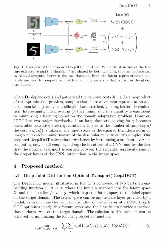
Fig. 1. Overview of the proposed DeepJDOT method. While the structure of the fea-ture extractor g and the classifier f are shared by both domains, they are representedtwice to distinguish between the two domains. Both the latent representations andlabels are used to compute per batch a coupling matrix γ that is used in the globalloss function.

where Df depends on f and gathers all the pairwise costs d(·, ·). As a by-productof this optimization problem, samples that share a common representation anda common label (through classification) are matched, yielding better discrimina-tion. Interestingly, it is proven in [5] that minimizing this quantity is equivalentto minimizing a learning bound on the domain adaptation problem. However,JDOT has two major drawbacks: i) on large datasets, solving for γ becomesintractable because γ scales quadratically in size to the number of samples; ii)the cost c(xsi ,x

tj) is taken in the input space as the squared Euclidean norm on

images and can be uninformative of the dissimilarity between two samples. Ourproposed DeepJDOT solves those two issues by introducing a stochastic versioncomputing only small couplings along the iterations of a CNN, and by the factthat the optimal transport is learned between the semantic representations inthe deeper layers of the CNN, rather than in the image space.

4 Proposed method

4.1 Deep Joint Distribution Optimal Transport(DeepJDOT)

The DeepJDOT model, illustrated in Fig. 1, is composed of two parts: an em-bedding function g : x → z, where the input is mapped into the latent spaceZ, and the classifier f : z → y, which maps the latent space to the label spaceon the target domain. The latent space can be any feature layer provided by amodel, as in our case the penultimate fully connected layer of a CNN. DeepJ-DOT optimizes jointly this feature space and the classifier to provide a methodthat performs well on the target domain. The solution to this problem can beachieved by minimizing the following objective function:

minγ∈Π(µs,µt),f,g

∑i

∑j

γijd(g(xsi ),y

si ; g(xtj), f(g(xtj))

), (5)


where d(g(xsi ),y

si ; g(xtj), f(g(xtj)

)= α‖g(xsi )−g(xtj)‖2 +λtL

(ysi , f(g(xtj))

), and

α and λt are the parameters controlling the tradeoff between the two terms, asin equation (3). Similarly to JDOT, the first term in the loss compares the com-patibility of the embeddings for the source and target domain, while the secondterm considers the classifier f learned in the target domain and its regularitywith respect to the labels available in the source. Despite similarities with theformulation of JDOT [5], our proposition comes with the notable difference that,in DeepJDOT, the Wasserstein distance is minimized between the joint (embed-ded space/label) distributions within the CNN, rather than between the originalinput spaces. As the deeper layers of a CNN encode both spatial and semanticinformation, we believe them to be more apt to describe the image content forboth domains, rather than the original features that are affected by a numberof factors such as illumination, pose or relative position of objects.

One can note that the formulation reported in equation (5) only depends onthe classifier learned in the target domain. By doing so, one puts the emphasis onlearning a good classifier for the target domain, and disregards the performanceof the classifier when considering source samples. In recent literature, such adegradation in the source domain has been named as ‘catastrophic forgetting ’ [33,34]. To avoid such forgetting, one can easily re-incorporate the loss on the sourcedomain in (5), leading to the final DeepJDOT objective:

minγ,f,g

1

ns

∑i

Ls (ysi , f(g(xsi )))+∑i,j

γij(α‖g(xsi )− g(xtj)‖2 + λtLt

(ysi , f(g(xtj))

)).

(6)This last formulation is the optimization problem solved by DeepJDOT. How-ever, for large sample sizes the constraint of computing a full γ yields a com-putationally infeasible problem, both in terms of memory and time complexity.In the next section, we propose an approximation method based on stochasticoptimization.

4.2 Solving the optimization problem with stochastic gradients

In this section, we describe the approximate optimization procedure for solvingDeepJDOT. Equation (6) involves two groups of variables to be optimized: theOT matrix γ and the models f and g. This suggest the use of an alternativeminimization approach (as proposed in the original JDOT). Indeed, when g and

f are fixed, solving equation (6) boils down to a standard OT problem with as-

sociated cost matrix Cij = α‖g(xsi )− g(xtj)‖2 +λtLt

(ysi , f(g(xtj))

). When fixing

γ, optimizing g and f is a classical deep learning problem. However, comput-ing the optimal coupling with the classical OT solvers is not scalable to large-scale datasets. Despite some recent development for large scale OT with generalground loss [31, 32], the model does not scale sufficiently to meet requirementsof recent computer vision tasks.

Therefore, in this work we propose to solve the problem with a stochasticapproximation using minibatches from both the source and target domains [35].

DeepJDOT 7

This approach has two major advantages: it is scalable to large datasets andcan be easily integrated in modern deep learning frameworks. More specifically,the objective function (6) is approximated by sampling a mini-batch of size m,leading to the following optimization problem:

minf,g

E

[1

m

m∑i=1

Ls (ysi , f(g(xsi )) + minγ∈∆

m∑i,j


(ysi , f(g(xtj))

))](7)

where E is the expected value with respect to the randomly sampled mini-batches drawn from both source and target domains. The classification loss func-tions for the source (Ls) and target (Lt) domains can be any general class of lossfunctions that are twice differentiable. We opted for a traditional cross-entropyloss in both cases. Note that, as discussed in [35], the expected value over theminibtaches does not converge to the true OT coupling between every pair ofsamples, which might then lead to the appearance of connections between sam-ples that would not have been connected in the full coupling. However, this canalso be seen as a regularization that will promote sharing of the mass betweenneighboring samples. Finally note that we did not use the regularized versionof OT as in [35], since it introduces an additional regularization parameter thatshould be cross-validated, which can make the model calibration even more com-plex. Still, the extension of DeepJDOT to regularized OT is straightforward andcould be beneficial for high-dimensional embeddings g.

Consequently, we propose to obtain the stochastic update for Eq.(7) as follows(and summarized in Algorithm 4):

1. With fixed CNN parameters (g, f) and for every randomly drawn minibatch(of m samples), obtain the coupling

minγ∈Π(µs,µt)

m∑i,j=1

γij

(α‖g(xsi )− g(xtj)‖2 + λtLt

(ysi , f(g(xtj))

))(8)

using the network simplex flow algorithm.

2. With fixed coupling γ obtained at the previous step, update the embed-ding function (g) and classifier (f) with stochastic gradient update for thefollowing loss on the minibatch:

1

m

m∑i=1

Ls (ysi , f(g(xsi )))+

m∑i,j=1


(ysi , f(g(xtj))

)).

(9)The domain alignment term aligns only the source and target samples withsimilar activation/labels and the sparse matrix γ will automatically performlabel propagation between source and target samples. The classifier f issimultaneously learnt in both source and target domain.


Algorithm 1 DeepJDOT stochastic optimization

Require: xs: source domain samples, xt: target domain samples, ys: source domainlabels

1: for each batch of source (xbs,yb

s) and target samples (xbt) do

2: fix g and f , solve for γ as in equation (8)3: fix γ, and update for g and f according to equation (9)4: end for

5 Experiments and Results

We evaluate DeepJDOT on three adaptation tasks: digits classification (Sec-tion 5.1), the OfficeHome dataset (Section 5.2), and the Visual Domain Adapta-tion challenge (visDA; Section 5.3). For each dataset, we first present the data,then detail the implementation and finally present and discuss the results.

5.1 Digit classification

Datasets We consider four data sources (domains) from the digits classificationfield: MNIST [36], USPS [37], MNIST-M, and the Street View House Numbers(SVHN) [38] dataset. Each dataset involves a 10-class classification problem(retrieving numbers 0-9):

- USPS. The USPS datasets contains 7‘291 training and 2‘007 test grayscaleimages of handwritten images, each one of size 16× 16 pixels.

- MNIST. The MNIST dataset contains 60‘000 training and 10‘000 testinggrayscale images of size 28 × 28.

- MNIST M. We generated the MNIST-M images by following the protocolin [8]. MNIST-M is a variation on MNIST, where the (black) backgroundis replaced by random patches extracted from the Berkeley SegmentationData Set (BSDS500) [39]. The number of training and testing samples arethe same as the MNIST dataset discussed above.

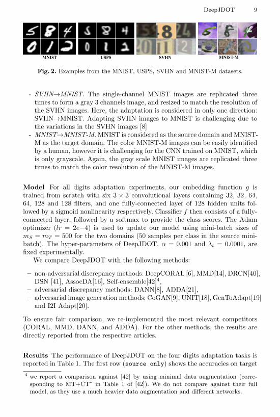
- SVHN. The SVHN dataset contains house numbers extracted from GoogleStreet View images. We used the Format2 version of SVHN, where the im-ages are cropped into 32 × 32 pixels. Multiple digits can appear in a singleimage, the objective is to detect the digit in the center of the image. Thisdataset contains 73‘212 training images, and 26‘032 testing images of size32× 32×3. The respective examples of the each dataset is shown in Figure2.

The three following experiments were run (the arrow direction corresponds tothe sense of the domain adaptation):

- USPS↔MNIST. The USPS images are zero-padded to reach the same sizeas MNIST dataset. The adaptation is considered in both directions: USPS→ MNIST, and MNIST → USPS.

DeepJDOT 9

Fig. 2. Examples from the MNIST, USPS, SVHN and MNIST-M datasets.

- SVHN→MNIST. The single-channel MNIST images are replicated threetimes to form a gray 3 channels image, and resized to match the resolution ofthe SVHN images. Here, the adaptation is considered in only one direction:SVHN→MNIST. Adapting SVHN images to MNIST is challenging due tothe variations in the SVHN images [8]

- MNIST→MNIST-M. MNIST is considered as the source domain and MNIST-M as the target domain. The color MNIST-M images can be easily identifiedby a human, however it is challenging for the CNN trained on MNIST, whichis only grayscale. Again, the gray scale MNIST images are replicated threetimes to match the color resolution of the MNIST-M images.

Model For all digits adaptation experiments, our embedding function g istrained from scratch with six 3 × 3 convolutional layers containing 32, 32, 64,64, 128 and 128 filters, and one fully-connected layer of 128 hidden units fol-lowed by a sigmoid nonlinearity respectively. Classifier f then consists of a fully-connected layer, followed by a softmax to provide the class scores. The Adamoptimizer (lr = 2e−4) is used to update our model using mini-batch sizes ofmS = mT = 500 for the two domains (50 samples per class in the source mini-batch). The hyper-parameters of DeepJDOT, α = 0.001 and λt = 0.0001, arefixed experimentally.

We compare DeepJDOT with the following methods:

– non-adversarial discrepancy methods: DeepCORAL [6], MMD[14], DRCN[40],DSN [41], AssocDA[16], Self-ensemble[42]4,

– adversarial discrepancy methods: DANN[8], ADDA[21],– adversarial image generation methods: CoGAN[9], UNIT[18], GenToAdapt[19]

and I2I Adapt[20].

To ensure fair comparison, we re-implemented the most relevant competitors(CORAL, MMD, DANN, and ADDA). For the other methods, the results aredirectly reported from the respective articles.

Results The performance of DeepJDOT on the four digits adaptation tasks isreported in Table 1. The first row (source only) shows the accuracies on target

4 we report a comparison against [42] by using minimal data augmentation (corre-sponding to MT+CT∗ in Table 1 of [42]). We do not compare against their fullmodel, as they use a much heavier data augmentation and different networks.


test data achieved with classifiers trained on source data without adaptation,and the row (target only) reports accuracies on the target test data achievedwith classifiers trained on the target training data. This method is considered asan upper bound for our proposed method and can be seen as our gold standard.StochJDOT (stochastic adaptation of JDOT) refers to the accuracy of our pro-posed method, when the discrepancy between source and target domain is com-puted with an `2 distance in the original image space. Lastly, DeepJDOT-sourceindicates the source data accuracy, after adapting to the target domain, and canbe considered a measure of catastrophic forgetting.

The experimental results show that DeepJDOT achieves accuracies compa-rable or higher to the current state-of-the-art methods. When the methods inthe first block of Table 1 are considered, DeepJDOT outperforms the competi-tors by large margins, with the exception of DANN that have similar perfor-mance on the MNIST→USPS task. In the more challenging adaptation settings(SVHN→MNIST and MNIST→MNIST-M), the state-of-the-art methods5 werenot able to adapt well to the target domain. Next, when the methods in the sec-ond block of Table 1 is considered, our method showed impressive performance,despite DeepJDOT not using any complex procedure for generating target imagesto perform the adaptation.

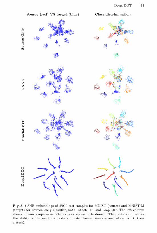
t-SNE embeddings We visualize the quality of the embeddings for the sourceand target domain learnt by DeepJDOT, StochJDOT and DANN using t-SNE embed-ding on the MNIST→MNIST-M adaptation task (Figure 3). As expected, in thesource model the samples from the source domain are well clustered and targetsamples are more scattered. The t-SNE embeddings with the DANN were not ableto align the distributions well, and this observation also holds for StochJDOT. Itis noted that StochJDOT does not align the distributions, but learns the classi-fier in target domain directly. The poor embeddings of the target samples withStochJDOT shows the necessity of computing the ground metric (cost function) ofoptimal transport in the deep CNN layers. Finally, DeepJDOT perfectly aligns thesource domain samples and target domain samples to each other, which explainsthe good numerical performances reported above. The “tentacle”-shaped andnear-perfect separation of the classes in the embedding illustrate the fact thatDeepJDOT finds an embedding that both aligns the source/target distribution,but also maximizes the margin between the classes.

Ablation study Table 2 reports the results obtained in the USPS→MNISTand MNIST→ MNIST-M cases for models using only parts of our proposedloss (equation (6)). When only the JDOT loss is considered (αd+ Lt case), theaccuracy drops in both adaptation cases. This behavior might be due to overfit-ting of the target classifier to the noisy pseudo- (propagated) labels. However,the performance is comparable to non-adversarial discrepancy-based methods

5 For ADDA[21] in the SVHN→MNIST adaptation task the accuracy is reported fromthe paper, as we were not able to further improve the source only accuracy

DeepJDOT 11

Source (red) VS target (blue) Class discrimination

Sourc

eOnly

DANN

Sto

chJDOT

DeepJDOT

Fig. 3. t-SNE embeddings of 2‘000 test samples for MNIST (source) and MNIST-M(target) for Source only classifier, DANN, StochJDOT and DeepJDOT. The left columnshows domain comparisons, where colors represent the domain. The right column showsthe ability of the methods to discriminate classes (samples are colored w.r.t. theirclasses).


Table 1. Classification accuracy on the target test datasets for the digit classificationtasks. Source only and target only refer to training on the respective datasets withoutdomain adaptation and evaluating on the target test dataset. The accuracies reportedin the first block are our own implementations, while the second block reports perfor-mances from the respective articles. Bold and italic indicates the best and second bestresults. The last line reports the performance of DeepJDOT on the source domain.

MethodAdaptation:source→target

MNIST → USPS USPS → MNIST SVHN → MNIST MNIST → MNIST-M

Source only 94.8 59.6 60.7 60.8

DeepCORAL [6] 89.33 91.5 59.6 66.5MMD [14] 88.5 73.5 64.8 72.5DANN [8] 95.7 90.0 70.8 75.4ADDA [21] 92.4 93.8 76.05 78.8

AssocDA [16] - - 95.7 89.5Self-ensemble4[42] 88.14 92.35 93.33 -

DRCN [40] 91.8 73.6 81.9 -DSN [41] 91.3 - 82.7 83.2

CoGAN [9] 91.2 89.1 - -UNIT [18] 95.9 93.5 90.5 -

GenToAdapt [19] 95.3 90.8 92.4 -I2I Adapt [20] 92.1 87.2 80.3 -

StochJDOT 93.6 90.5 67.6 66.7DeepJDOT (ours) 95.7 96.4 96.7 92.4

target only 95.8 98.7 98.7 96.8

DeepJDOT-source 98.5 94.9 75.7 97.8

Table 2. Ablation study of DeepJDOT.

Method USPS → MNIST MNIST → MNIST-M

Ls + (αd+ Lt) 96.4 92.4αd+ Lt 86.41 73.6Ls + αd 95.53 82.3

reported in Table 1. On the contrary, when only the feature space distribution isincluded in Equation (6), i.e. the Ls+αd experiment, the accuracy is close to ourfull model in USPS→MNIST direction, but drops in the MNIST→ MNIST-Mone. Overall the accuracies are improved compared to the original JDOT model,which highlights the importance of including the information from the source do-main. Moreover, this also highlights the importance of simultaneously updatingthe classifier both in the source and target domain. Summarizing, this ablationstudy showed that the individual components bring complimentary informationto achieve the best classification results.

5.2 Office-Home

Dataset The Office-Home dataset [43] contains around 15′500 images in 65categories from four different domains: artistic paintings, clipart, product andreal-world images.

DeepJDOT 13

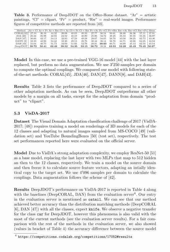
Table 3. Performance of DeepJDOT on the Office-Home dataset. “Ar” = artisticpaintings, “Cl” = clipart, “Pr” = product, “Rw” = real-world images. Performancefigures of competitive methods are reported from [43].

Method Ar→ Cl Ar→ Pr Ar→ Rw Cl→ Ar Cl→ Pr Cl→ Rw Pr→Ar Pr→Cl Pr→Rw Rw→Ar Rw→Cl Rw→Pr MeanCORAL[45] 27.10 36.16 44.32 26.08 40.03 40.33 27.77 30.54 50.61 38.48 36.36 57.11 37.91JDA [46] 25.34 35.98 42.94 24.52 40.19 40.90 25.96 32.72 49.25 35.10 35.35 55.35 36.97DAN [47] 30.66 42.17 54.13 32.83 47.59 49.58 29.07 34.05 56.70 43.58 38.25 62.73 43.46DANN [8] 33.33 42.96 54.42 32.26 49.13 49.76 30.44 38.14 56.76 44.71 42.66 64.65 44.94DAH [43] 31.64 40.75 51.73 34.69 51.93 52.79 29.91 39.63 60.71 44.99 45.13 62.54 45.54DeepJDOT 39.73 50.41 62.49 39.52 54.35 53.15 36.72 39.24 63.55 52.29 45.43 70.45 50.67

Model In this case, we use a pre-trained VGG-16 model [44] with the last layerreplaced, but perform no data augmentation. We use 3′250 samples per domainto compute the optimal couplings. We compared our model with following state-of-the-art methods: CORAL[45], JDA[46], DAN[47], DANN[8], and DAH[43].

Results Table 3 lists the performance of DeepJDOT compared to a series ofother adaptation methods. As can be seen, DeepJDOT outperforms all othermodels by a margin on all tasks, except for the adaptation from domain “prod-uct” to “clipart”.

5.3 VisDA-2017

Dataset The Visual Domain Adaptation classification challenge of 2017 (VisDA-2017; [48]) requires training a model on renderings of 3D models for each of the12 classes and adapting to natural images sampled from MS-COCO [49] (vali-dation set) and YouTube BoundingBoxes [50] (test set), respectively. The testset performances reported here were evaluated on the official server.

Model Due to VisDA’s strong adaptation complexity, we employ ResNet-50 [51]as a base model, replacing the last layer with two MLPs that map to 512 hiddenan then to the 12 classes, respectively. We train a model on the source domainand then freeze it to calculate source feature vectors, adapting an intially iden-tical copy to the target set. We use 4′096 samples per domain to calculate thecouplings. Data augmentation follows the scheme of [42].

Results DeepJDOT’s performance on VisDA-2017 is reported in Table 4 alongwith the baselines (DeepCORAL, DAN) from the evaluation server6. Our entryin the evaluation server is mentioned as oatmil. We can see that our methodachieved better accuracy than the distribution matching methods (DeepCORAL[6], DAN [47]) with all the classes, expect knife. We observe a negative transferfor the class car for DeepJDOT, however this phenomena is also valid with themost of the current methods (see the evaluation server results). For a fair com-parison with the rest of the methods in the evaluation server, we also showed(values in bracket of Table 4) the accuracy difference between the source model

6 https://competitions.codalab.org/competitions/17052#results


Table 4. Performance of DeepJDOT on the VisDA 2017 classification challenge. Thescores in the bracket indicate the accuracy difference between the source (unadapted)model and target (adapted) model. The respective values of CORAL and DAN arereported from the evaluation server 6.

Method plane bcycl bus car horse knife mcycl person plant sktbd train truck MeanSource only 36.0 4.0 19.9 94.7 14.8 0.42 38.7 3.8 37.4 8.1 71.9 6.7 28.0

DeepCORAL [6] 62.5 21.7 66.3 64.6 31.1 36.7 54.2 24.9 73.8 29.9 43.4 34.2 45.3 (19.0)DAN [47] 55.3 18.4 59.8 68.6 55.3 41.4 63.4 30.4 78.8 23.0 62.9 40.2 49.8 (19.5)DeepJDOT 85.4 50.4 77.3 87.3 69.1 14.1 91.5 53.3 91.9 31.2 88.5 61.8 66.9 (38.9)

and target model. Our method is ranked sixth when the mean accuracy is consid-ered, and third when the difference between the source model and target modelis considered at the time of publication. It is noted that the performance of ourmethod depends on the capacity of the source model: if a larger CNN is used,the performance of our method could be improved further.

6 Conclusions

In this paper, we proposed the DeepJDOT model for unsupervised deep domainadaptation based on optimal transport. The proposed method aims at learninga common latent space for the source and target distributions, that conveys dis-criminant information for both domains. This is achieved by minimizing the dis-crepancy of joint deep feature/labels domain distributions by means of optimaltransport. We propose an efficient stochastic algorithm that solves this problem,and despite being simple and easily integrable into modern deep learning frame-works, our method outperformed the state-of-the-art on cross domain digits andoffice-home adaptation, and provided satisfactory results on the VisDA-2017adaptation.

Future works will consider the evaluation of this method in multi-domainsscenario, as well as more complicated cost functions taking into account simi-larities of the representations across the embedding layers and/or similarities oflabels across different classifiers.

Acknowledgement

This work benefited from the support of Region Bretagne grant and OATMILANR-17-CE23-0012 project of the French National Research Agency (ANR). Wegratefully acknowledge the support of NVIDIA Corporation with the donationof the Titan Xp GPU used for this research. The constructive comments andsuggestions of anonymous reviewers are gratefully acknowledged.

References

1. Patel, V.M., Gopalan, R., Li, R., Chellappa, R.: Visual domain adaptation: asurvey of recent advances. IEEE SPM 32(3) (2015) 53–69

DeepJDOT 15

2. Saenko, K., Kulis, B., Fritz, M., Darrell, T.: Adapting visual category models tonew domains. In: ECCV. (2010) 213–226

3. Gopalan, R., Li, R., Chellappa, R.: Domain adaptation for object recognition: Anunsupervised approach. In: ICCV. (2011) 999–1006

4. Courty, N., Flamary, R., Tuia, D., Rakotomamonjy, A.: Optimal transport fordomain adaptation. IEEE TPAMI 39(9) (2017) 1853–1865

5. Courty, N., Flamary, R., Habrard, A., Rakotomamonjy, A.: Joint distributionoptimal transportation for domain adaptation. In: NIPS. (2017)

6. Sun, B., Saenko, K.: Deep coral: Correlation alignment for deep domain adaptation.In: ECCV workshops. (2016) 443–450

7. Luo, Z., Zou, Y., Hoffman, J., Fei-Fei, L.: Label efficient learning of transferablerepresentations across domains and tasks. In: NIPS. (2017)

8. Ganin, Y., Ustinova, E., Ajakan, H., Germain, P., Larochelle, H., Laviolette, F.,Marchand, M., Lempitsky, V.: Domain-adversarial training of neural networks. J.Mach. Learn. Res. 17(1) (January 2016) 2096–2030

9. Liu, M.Y., Tuzel, O.: Coupled generative adversarial networks. In Lee, D.D.,Sugiyama, M., Luxburg, U.V., Guyon, I., Garnett, R., eds.: NIPS. (2016) 469–477

10. Ben-David, S., Blitzer, J., Crammer, K., Pereira, F.: Analysis of representationsfor domain adaptation. In: NIPS. (2007) 137–144

11. Jhuo, I.H., Liu, D., Lee, D.T., Chang, S.F.: Robust visual domain adaptation withlow-rank reconstruction. In: CVPR. (2012) 2168–2175

12. Hoffman, J., Rodner, E., Donahue, J., Saenko, K., Darrell, T.: Efficient learningof domain-invariant image representations. In: ICLR. (2013)

13. Aljundi, R., Tuytelaars, T.: Lightweight unsupervised domain adaptation by con-volutional filter reconstruction. In: ECCV. (2016)

14. Long, M., Cao, Y., Wang, J., Jordan, M.I.: Learning transferable features withdeep adaptation networks. In: ICML. (2015) 97–105

15. Long, M., Wang, J., Jordan, M.I.: Unsupervised domain adaptation with residualtransfer networks. In: NIPS. (2016)

16. Haeusser, P., Frerix, T., Mordvintsev, A., Cremers, D.: Associative domain adap-tation. In: ICCV. (2017)

17. Tzeng, E., Hoffman, J., Darrell, T., Saenko, K.: Simultaneous deep transfer acrossdomains and tasks. In: ICCV. (2015)

18. Liu, M.Y., Breuel, T., Kautz, J.: Unsupervised image-to-image translation net-works. In Guyon, I., Luxburg, U.V., Bengio, S., Wallach, H., Fergus, R., Vish-wanathan, S., Garnett, R., eds.: NIPS. (2017) 700–708

19. Sankaranarayanan, S., Balaji, Y., Castillo, C.D., Chellappa, R.: Generate to adapt:Aligning domains using generative adversarial networks. CoRR abs/1704.01705(2017)

20. Murez, Z., Kolouri, S., Kriegman, D., Ramamoorthi, R., Kim, K.: Image to ImageTranslation for Domain Adaptation. ArXiv e-prints (December 2017)

21. Tzeng, E., Hoffman, J., Darrell, T., Saenko, K.: Adversarial discriminative domainadaptation. In: CVPR. (2017)

22. Monge, G.: Memoire sur la theorie des deblais et des remblais. De l’ImprimerieRoyale (1781)

23. Kantorovich, L.: On the translocation of masses. C.R. (Doklady) Acad. Sci. URSS(N.S.) 37 (1942) 199–201

24. Villani, C.: Optimal transport: old and new. Grundlehren der mathematischenWissenschaften. Springer (2009)

25. Courty, N., Flamary, R., Tuia, D.: Domain adaptation with regularized optimaltransport. In: ECML. (2014)


26. Perrot, M., Courty, N., Flamary, R., Habrard, A.: Mapping estimation for discreteoptimal transport. In: NIPS. (2016) 4197–4205

27. Redko, I., Habrard, A., Sebban, M.: Theoretical analysis of domain adaptationwith optimal transport. In: ECML/PKDD. (2017) 737–753

28. Shen., J., Qu, Y., Zhang, W., Yu, Y.: Wasserstein distance guided representationlearning for domain adaptation. In: AAAI. (2018)

29. Arjovsky, M., Chintala, S., Bottou, L.: Wasserstein generative adversarial networks.In: ICML. (2017) 214–223

30. Cuturi, M.: Sinkhorn distances: Lightspeed computation of optimal transportation.In: NIPS. (2013) 2292–2300

31. Genevay, A., Cuturi, M., Peyre, G., Bach, F.: Stochastic optimization for large-scale optimal transport. In: NIPS. (2016) 3432–3440

32. Seguy, V., Damodaran, B, B., Flamary, R., Courty, N., Rolet, A., Blondel, M.:Large-scale optimal transport and mapping estimation. In: ICLR. (2018)

33. Shmelkov, K., Schmid, C., Alahari, K.: Incremental learning of object detectorswithout catastrophic forgetting. In: ICCV, Venice, Italy (2017)

34. Li, Z., Hoiem, D.: Learning without forgetting. IEEE TPAMI (in press)35. Genevay, A., Peyre, G., Cuturi, M.: Sinkhorn-autodiff: Tractable wasserstein learn-

ing of generative models. arXiv preprint arXiv:1706.00292 (2017)36. Lecun, Y., Bottou, L., Bengio, Y., Haffner, P.: Gradient-based learning applied to

document recognition. Proceedings of the IEEE 86(11) (Nov 1998) 2278–232437. Hull, J.J.: A database for handwritten text recognition research. IEEE TPAMI

16(5) (May 1994) 550–55438. Netzer, Y., Wang, T., Coates, A., Bissacco, A., Wu, B., Ng, A.Y.: Reading digits

in natural images with unsupervised feature learning. In: NIPS worksophs. (2011)39. Arbelaez, P., Maire, M., Fowlkes, C., Malik, J.: Contour detection and hierarchical

image segmentation. IEEE TPAMI 33(5) (May 2011) 898–91640. Ghifary, M., Kleijn, W.B., Zhang, M., Balduzzi, D., Li, W.: Deep reconstruction-

classification networks for unsupervised domain adaptation. In: ECCV. (2016)597–613

41. Bousmalis, K., Trigeorgis, G., Silberman, N., Krishnan, D., Erhan, D.: Domainseparation networks. In: NIPS. (2016) 343–351

42. French, G., Mackiewicz, M., Fisher, M.: Self-ensembling for visual domain adap-tation. In: International Conference on Learning Representations. (2018)

43. Venkateswara, H., Eusebio, J., Chakraborty, S., Panchanathan, S.: Deep hashingnetwork for unsupervised domain adaptation. In: (IEEE) Conference on ComputerVision and Pattern Recognition (CVPR). (2017)

44. Simonyan, K., Zisserman, A.: Very deep convolutional networks for large-scaleimage recognition. arXiv preprint arXiv:1409.1556 (2014)

45. Sun, B., Feng, J., Saenko, K.: Return of frustratingly easy domain adaptation. In:Proceedings of the Thirtieth AAAI Conference on Artificial Intelligence. AAAI’16,AAAI Press (2016) 2058–2065

46. Long, M., Wang, J., Ding, G., Sun, J., Yu, P.S.: Transfer feature learning withjoint distribution adaptation. In: 2013 IEEE International Conference on ComputerVision. (Dec 2013) 2200–2207

47. Long, M., Cao, Y., Wang, J., Jordan, M.: Learning transferable features with deepadaptation networks. In Bach, F., Blei, D., eds.: Proceedings of the 32nd Inter-national Conference on Machine Learning. Volume 37 of Proceedings of MachineLearning Research., Lille, France, PMLR (07–09 Jul 2015) 97–105

48. Peng, X., Usman, B., Kaushik, N., Hoffman, J., Wang, D., Saenko, K.: Visda: Thevisual domain adaptation challenge (2017)

DeepJDOT 17

49. Lin, T.Y., Maire, M., Belongie, S., Hays, J., Perona, P., Ramanan, D., Dollar, P.,Zitnick, C.L.: Microsoft coco: Common objects in context. In: European conferenceon computer vision, Springer (2014) 740–755

50. Real, E., Shlens, J., Mazzocchi, S., Pan, X., Vanhoucke, V.: Youtube-boundingboxes: A large high-precision human-annotated data set for object de-tection in video. In: Computer Vision and Pattern Recognition (CVPR), 2017IEEE Conference on, IEEE (2017) 7464–7473

51. He, K., Zhang, X., Ren, S., Sun, J.: Deep residual learning for image recognition.In: Proceedings of the IEEE conference on computer vision and pattern recognition.(2016) 770–778

deepjdot: deep joint distribution optimal transport for ... · deepjdot: deep joint distribution...

Documents