deep-space optical transceiver uplink detection … optical transceiver uplink detection analysis...
TRANSCRIPT
IPN Progress Report 42-193 • May 15, 2013
Deep-Space Optical Transceiver Uplink DetectionAnalysis
Andre Tkacenko∗, Kevin J. Quirk∗, and Meera Srinivasan∗
In this article, we develop and analyze an uplink signal detection technique for the
Deep-Space Optical Transceiver (DOT). Here, the detection is carried out using a set of
test statistics obtained from up-down counter (UDC) photon detection systems.
Specifically, we address two sets of statistics: the count outputs from a bank of uniformly
temporally spaced UDCs as well as the counts from a single UDC that cycles through
multiple uniformly spaced timing phases. From these test statistics, we derive the
Neyman-Pearson decision rule under certain input conditions and analyze the performance
of this hypothesis test. We show the performance trade-offs associated with both sets of
test statistics, which can then be used to determine which set to use as well as the number
of UDCs or timing phases required for implementation.
I. Introduction
In order to receive an uplink communication from an Earth-based beacon, the Deep-Space
Optical Transceiver (DOT) flight terminal will use a focal plane array [1] of photon
counting detector pixels (possibly of size 128× 128). While the Earth and beacon together
will occupy a varying amount of pixels depending upon the distance between the DOT and
Earth, the system is designed for the beacon to occupy a certain minimum region of pixels
(possibly 2× 2). This is illustrated in Figure 1.
For spatial acquisition, the DOT flight terminal will employ up-down counter (UDC)
photon detection systems at each pixel. Using UDCs provides a low complexity detection
method when combined with appropriate modulation to be able to distinguish between
uplink telemetry from the beacon on Earth and background illumination from the Earth
as well as ambient background illumination. When a telemetry waveform is incident on a
∗Communications Architectures and Research Section
The research described in this publication was carried out by the Jet Propulsion Laboratory, California
Institute of Technology, under a contract with the National Aeronautics and Space Administration. c© 2013
California Institute of Technology. U. S. Government sponsorship acknowledged.
1

uplink
beacon
… …
……
……
……
… …
…
…
Earth
Figure 1. DOT focal plane array with Earth and the uplink beacon present.
pixel, the UDCs will tend to yield a non-zero output, whereas when only background
illumination is received, the UDCs will have a zero net count on average. As the symbol
timing offset of the uplink beacon telemetry waveform will not be known to the DOT a
priori, UDC count statistics at several timing phases will be required in general. Two ways
in which this can be accommodated and which we will analyze here are as follows. Either
a bank of uniformly temporally spaced UDCs can be used or a single UDC can be used
multiple times at uniformly spaced timing phases. For either case, the temporal spacing is
with respect to the uplink symbol interval, which is assumed to be known at the DOT.
A. Outline
In Section I-B, we describe the notations that will be used in this article, whereas in
Section I-C, we provide a convenient list of terms that will be used throughout the article.
An overview of the uplink detection signal model that we will be focusing on here is
provided in Section II. In Section III, we detail the UDC test statistics that will be
considered here and introduce the chip interval counts used to canonically describe them.
The probabilistic modeling of the chip interval counts is derived in Section III-A, which is
then used to determine the probabilistic modeling of the multiple UDC, single phase and
single UDC, multiple phase statistics in Sections III-B and III-C, respectively. A
description of the Neyman-Pearson hypothesis test that will be used for detection is given
in Section IV, along with a symbol timing offset conditional variant as detailed in Section
IV-A. In Section V, we analyze several important special cases of the unconditional
Neyman-Pearson hypothesis test, including the single UDC, single phase case in Section
V-A, the dual UDC, single phase case in Section V-B, and the single UDC, dual phase
case in Section V-C. There, we see the difficulties in deriving the unconditional
Neyman-Pearson hypothesis test in general and shift our focus to detection tests
conditioned on the symbol timing offset. Specifically, in Section VI, we analyze the
detection performance for a worst case scenario (WCS) symbol timing offset for both the
multiple UDC, single phase system in Section VI-A as well as the single UDC, multiple
phase system in Section VI-B. In Section VII, we touch on some of the pros and cons
between the two proposed UDC-based uplink signal detection schemes. Concluding
remarks are made in Section VIII. Finally, in the Appendix, we simplify a certain
multivariate Gaussian distribution [2] integral over a hyperspherical region, a result which
2
is used to assess the WCS symbol timing offset detection performance.
B. Notations
Most notations are as in [2]. In particular, parentheses and subscripts are respectively used
to denote continuous and discrete function arguments. For example, g(x) would denote a
continuous function for x ∈ R, whereas hn would denote a discrete function for n ∈ Z.
Vector/matrix notations are as in [3]. Specifically, boldface lowercase letters (such as v) are
used to denote vectors, whereas boldface uppercase letters (such as A) represent matrices.
The k-th component of a vector v will be denoted [v]k, whereas the (k, `)-th element of a
matrix A is denoted as [A]k,`. In addition, the transpose operator will be represented by
the superscript T and the determinant of a square matrix S is expressed as det (S).
Random variables are denoted via a non-italicized font, while instances of random variables
are expressed using an italicized font. As an example, v may denote a random variable,
whereas an instance of v would be expressed as v. Vectors are denoted using a bold font.
For example, v may denote a random vector, while v would denote an instance of v.
A probability density function (pdf) [2] will be denoted by the letter f subscripted by the
random variable or vector. For instance, fv(v) and fv(v) would denote pdfs of the random
variable v and random vector v, respectively.
The notation N(µ, σ2
)will be used to denote a random variable with a normal or
Gaussian distribution [2] with mean µ and variance σ2. If a random variable v has such a
distribution, we will write v ∼ N(µ, σ2
). We will use φ(x) and Φ(x) to respectively denote
the pdf and cumulative distribution function (cdf) [2] of the standard normal distribution
[2] (i.e., N (0, 1)). These are given by the following expressions [2]:
φ(x) ,1√2πe−
x2
2 , Φ(x) ,∫ x
−∞φ(y) dy =
1√2π
∫ x
−∞e−
y2
2 dy .
It can be shown that if x ∼ N(µ, σ2
)and fx(x) and Fx(x) denote, respectively, the pdf
and cdf of x, then we have [2]
fx(x) =1
σφ
(x− µσ
), Fx(x) = Φ
(x− µσ
). (1)
Similar to the univariate case, the notation Np(µ,Σ) will be used to denote a p× 1
random vector with a multivariate normal or Gaussian distribution [2] with p× 1 mean
vector µ and p× p covariance matrix Σ. If a random vector v has such a distribution, we
will write v ∼ Np(µ,Σ). In this case, we have [2]
fv(v) =1
(2π)p2 (det (Σ))
12
e−12 (v−µ)TΣ−1(v−µ) . (2)
Finally, we will use the notation zNCχ2(x; p, λ) to denote the cdf of a noncentral
chi-square distribution with p degrees of freedom and non-centrality parameter λ evaluated
3
at x [4]. In addition, we will use the notation z−1NCχ2(P ; p, λ) to denote the quantile
function [2] (i.e., the inverse of the cdf) of a noncentral chi-square distribution with p
degrees of freedom and non-centrality parameter λ evaluated at P .
C. Summary of Terms
A list of frequently used terms is provided below for convenience.
M − pulse position modulation (PPM) [1, 5] data symbol order,
P − number of inter-symbol guard time (ISGT) [6] slots used,
G − number of UDCs in a multiple UDC, single phase system or the number of
timing phases of a single UDC, multiple phase system,
λs − average detected signal photon arrival rate,
λb − average detected background and dark [1] photon arrival rate,
Ts − slot time interval,
Ks − mean number of signal photon counts per signal slot (i.e., Ks , λs (M + P )Ts),
Kb − mean number of background photon counts per slot (i.e., Kb , λbTs),
Nsym − number of symbols observed for a multiple UDC, single phase system,
Nspp − number of symbols per timing phase observed for a single UDC, multiple
phase system,
Tsym − symbol time interval (i.e., Tsym , (M + P )Ts),
Td − detection time interval (i.e., Td = NsymTsym for a multiple UDC, single phase
system and Td = NsppGTsym for a single UDC, multiple phase system).
II. Uplink Detection Signal Model
The uplink signal model is characterized by a received photon intensity function, which we
denote here by i(t). From UDC test statistics based upon this received signal, we must
infer whether or not telemetry has been sent. For the DOT, we assume that a transmitted
telemetry signal will consist of symbols, each formed from the concatenation of the
following components:
• an M -ary PPM data symbol,
• a set of P ISGTs.
Whether or not a telemetry signal was transmitted, we will assume that there is a
background illumination present at the receiver. This leads to the following expression for
4

bb
(M +P)n0(M +P)n0
²²
(M +P)n0 +M(M +P)n0 +M
00 11 · · ·· · · · · ·· · · M
|
1
M
|
1
P ISGTsP ISGTs
(M +P) (n0 +1)(M +P) (n0 +1)
00 11 · · ·· · · · · ·· · · M
|
1
M
|
1
(M +P) (n0 +1)+M(M +P) (n0 +1)+M (M +P) (n0 +2)(M +P) (n0 +2)
t
Ts
t
TsT
i(t)i(t)
s (M +P) + bs (M +P) + b
M-ary PPM data symbol
(only one slot is active per composite symbol)
M-MM ary PPM dataa a symbm ol
(only one slot is active per composite symbm ol)
Figure 2. Sample plot of the received photon intensity waveform i(t) when telemetry is present.
the received laser intensity waveform i(t):
i(t) =
λs (M + P )
[ ∞∑n=−∞
p
(t
Ts− ε− dn − (M + P )n
)]+ λb , telemetry present
λb , telemetry absent
,
(3)
where we have
ε , symbol timing offset (normalized by Ts),
In general, we have ε0 ≤ ε < ε0 + (M + P ) for any ε0 ∈ R.
{dn} , M -ary PPM data sequence,
Here, dn ∈ {0, 1, . . . ,M − 1}.
Also, we will assume that {dn} is an independent, identically distributed
(iid or i.i.d.) sequence [2] with
Pr {dn = m} =1
M, ∀ 0 ≤ m ≤M − 1, n ∈ Z .
p(x) , telemetry transmit pulse shape.
Here, we assume p(x) is rectangular as follows:
p(x) =
1 , 0 ≤ x < 1
0 , otherwise.
A sample plot of the received photon intensity signal i(t) in the case of telemetry being
present is shown in Figure 2. As only one of the M -ary PPM data slots will be active for
each composite symbol, consisting of (M + P ) slot intervals total, it follows that the
average signal arrival rate will be λs.
Another signal of interest which will simplify subsequent statistical analysis of the UDC
hypothesis test metrics will be the photon intensity function averaged over the random
PPM data. This signal, which we will denote by i(t), is given by the following expression:
i(t) = E{dn}[i(t)] =
λs
(M + P )
M
∞∑n=−∞
p
(tTs− ε− (M + P )n
M
)+ λb , telemetry present
λb , telemetry absent
.
(4)
5
(M +P) (n0 +2)(M +P) (n0 +2)(M +P) (n0 +1)+M(M +P) (n0 +1)+M
b b
(M +P)n0(M +P)n0
²²
(M +P)n0 +M(M +P)n0 +M
P ISGTsP ISGTs
(M +P) (n0 +1)(M +P) (n0 +1)
t
Ts
t
TsT
s(M+P )M
+ b s(M+P )M
+ b
i(t)i(t)data-averaged pulsedataa a-aa avaa eraged pulse
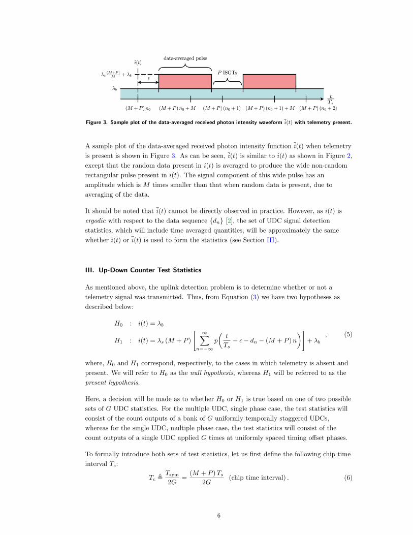
Figure 3. Sample plot of the data-averaged received photon intensity waveform i(t) with telemetry present.
A sample plot of the data-averaged received photon intensity function i(t) when telemetry
is present is shown in Figure 3. As can be seen, i(t) is similar to i(t) as shown in Figure 2,
except that the random data present in i(t) is averaged to produce the wide non-random
rectangular pulse present in i(t). The signal component of this wide pulse has an
amplitude which is M times smaller than that when random data is present, due to
averaging of the data.
It should be noted that i(t) cannot be directly observed in practice. However, as i(t) is
ergodic with respect to the data sequence {dn} [2], the set of UDC signal detection
statistics, which will include time averaged quantities, will be approximately the same
whether i(t) or i(t) is used to form the statistics (see Section III).
III. Up-Down Counter Test Statistics
As mentioned above, the uplink detection problem is to determine whether or not a
telemetry signal was transmitted. Thus, from Equation (3) we have two hypotheses as
described below:
H0 : i(t) = λb
H1 : i(t) = λs (M + P )
[ ∞∑n=−∞
p
(t
Ts− ε− dn − (M + P )n
)]+ λb
, (5)
where, H0 and H1 correspond, respectively, to the cases in which telemetry is absent and
present. We will refer to H0 as the null hypothesis, whereas H1 will be referred to as the
present hypothesis.
Here, a decision will be made as to whether H0 or H1 is true based on one of two possible
sets of G UDC statistics. For the multiple UDC, single phase case, the test statistics will
consist of the count outputs of a bank of G uniformly temporally staggered UDCs,
whereas for the single UDC, multiple phase case, the test statistics will consist of the
count outputs of a single UDC applied G times at uniformly spaced timing offset phases.
To formally introduce both sets of test statistics, let us first define the following chip time
interval Tc:
Tc ,Tsym
2G=
(M + P )Ts2G
(chip time interval) . (6)
6

Then, let us define the random variable Nk as follows:
Nk , # of photon counts over the time interval t ∈ [kTc, (k + 1)Tc) , ∀ k ∈ Z . (7)
From these count random variables, we form our G UDC test statistics for both the
multiple UDC, single phase and single UDC, multiple phase cases. Let Nsym and Nspp
denote, respectively, the number of symbols observed for the multiple UDC, single phase
case and the number of symbols per phase observed for the single UDC, multiple phase
case (see Section I-C). The UDC test statistics {g`}G−1`=0 for the two cases are then
g` ,
1
Nsym
Nsym−1∑q=0
(2G)−1∑r=0
(−1)br−`G cN(2G)q+r , (multiple UDC, single phase case)
1
Nspp
Nspp−1∑q=0
(2G)−1∑r=0
(−1)br−`G cN(2G)(q+`Nspp)+r , (single UDC, multiple phase case)
.
(8)
A pictorial view of how the UDC statistics are formed in both cases is shown for G = 3 in
Figure 4. As can be seen from Figure 4(a), for the multiple UDC, single phase case, the
statistics overlap in time, whereas from Figure 4(b), for the single UDC, multiple phase
case, there is no temporal overlap of the test statistics. For both cases, however, it is
evident that the test statistics represent G time intervals uniformly offset across the total
symbol interval length Tsym.
A comment is in order here regarding the single UDC, multiple phase test statistics from
Equation (8). By construction, these statistics span contiguous, non-overlapping time
intervals. Specifically, from Equations (8), (7), and (6), it can be seen that g` represents
up-down photon counts over the time interval t ∈ [`NsppTsym, (`+ 1)NsppTsym), the set of
which, for all `, is contiguous and non-overlapping. However, as will be seen subsequently
in Section III-C, the probabilistic characterization of this set of test statistics will be the
same as those for which the time intervals are only non-overlapping. Hence, instead of the
contiguous and non-overlapping single UDC, multiple phase statistics from Equation (8),
we could also use a set of test statistics that are only non-overlapping. In essence, there is
no loss of generality in assuming a contiguous form as in Equation (8) and this was merely
chosen as such here for notational simplicity.
For notational convenience, we will define the G× 1 random vector g to be the vector of
UDC test statistics given by
g ,[
g0 g1 · · · gG−1
]T. (9)
In accordance with the notational conventions adopted here (see Section I-B), we will
denote an instance of g by g.
A. Probabilistic Modeling of the Chip Interval Counts
The photon detection counting process [1] is assumed to be a Poisson process [2]. Let λk
denote the average arrival rate [1] corresponding to the chip count variable Nk. From
7

tTc
tTcTT
· · ·· · ·· · ·· · ·
g0g0
· · ·· · ·
tTc
tTcTT
· · ·· · ·
g1g1
· · ·· · · · · ·· · ·
tTc
tTcTT
g2g2
N6q0+5N6q0+5N6q0+4N6q0+4
N6q0+3N6q0+3N6q0+2N6q0+2N6q0+1N6q0+1
N6q0N6q0
N6q0N6q0 N6q0+1N6q0+1
N6q0+2N6q0+2 N6q0+3N6q0+3 N6q0+4N6q0+4
N6q0+5N6q0+5
N6q0N6q0 N6q0+1N6q0+1 N6q0+2N6q0+2
N6q0+3N6q0+3 N6q0+4N6q0+4 N6q0+5N6q0+5
(a)
g0g0
N6q0+5N6q0+5N6q0+4N6q0+4N6q0+3N6q0+3
N6q0+2N6q0+2N6q0+1N6q0qq +1N6q0N6q0 · · ·· · ·· · ·· · ·
g1g1
N6(q0+Nspp)+5N6(q0+NsNN pp)+5N6(q0+Nspp)+4N6(q0+NsNN pp)+4
N6(q0+Nspp)+3N6(q0+NsNN pp)+3N6(q0+Nspp)+2N6(q0+NsNN pp)+2N6(q0+Nspp)+1N6(q0+NsNN pp)+1
N6(q0+Nspp)N6(q0+NsNN pp)
· · ·· · · · · ·· · · · · ·· · · · · ·· · ·
tTctTcTT
g2g2
N6(q0+2Nspp)+5N6(q0+2NsNN pp)+5
N6(q0+2Nspp)+4N6(q0+2NsNN pp)+4N6(q0+2Nspp)+3N6(q0+2NsNN pp)+3N6(q0+2Nspp)+2N6(q0+2NsNN pp)+2
N6(q0+2Nspp)+1N6(q0+2NsNN pp)+1N6(q0+2Nspp)N6(q0+2NsNN pp)
(b)
Figure 4. Pictorial view of the formation of the UDC test statistics for G = 3: (a) multiple UDC, single
phase case and (b) single UDC, multiple phase case (up counts in green and down counts in red).
8
Equation (7), we have
λk ,1
Tc
∫ (k+1)Tc
kTc
i(t) dt , (10)
where i(t) is as in Equation (3). Conditioned on λk, it follows that Nk is Poisson with
mean λkTc. Specifically, this means that we have [2]
Pr {Nk = m |λk} =(λkTc)
me−(λkTc)
m!um , m ∈ Z ,
where um is the Heaviside step sequence [2]. Furthermore, as Nk and N` represent counts
across non-overlapping time intervals for all k 6= ` (as evidenced from Equation (7)), it
follows that Nk |λk and N` |λ` are independent for all k 6= `.
When telemetry is present, the arrival rate λk is a deterministic function of the symbol
timing offset ε, when averaged over the random PPM data. For the case in which
telemetry is absent, it follows that λk = λb and so it is trivially a deterministic function of
ε. Thus, analogously to Equation (10), if we define the average arrival rate λk(ε) for both
the null and present hypotheses as
λk(ε) ,1
Tc
∫ (k+1)Tc
kTc
i(t) dt , (11)
where i(t) is given by Equation (4), then we have
Nk | ε ∼ Poisson(λk(ε)Tc
). (12)
In other words, the random variable Nk | ε is Poisson with mean λk(ε)Tc. Furthermore, as
Nk and N` represent non-overlapping count time intervals for all k 6= `, it follows that
Nk | ε and N` | ε are independent for all k 6= `.
One noteworthy property of λk(ε) that can be deduced from Equations (11) and (4) is that
λk(ε) = λk mod (2G)(ε) , ∀ k ∈ Z . (13)
This follows from the fact that i(t) is periodic with period Tsym = (2G)Tc (for both
hypotheses) and that the integration region in Equation (11) is over an interval of length
Tc. This implies that there are at most (2G) distinct values of λk(ε) for fixed ε. As such,
from Equations (12) and (13), we have the following:
Nk | ε ∼ Poisson(λk mod (2G)(ε)Tc
). (14)
In other words, as k varies, the distribution of the count variable Nk, conditioned on the
symbol timing offset ε, is only a function of the remainder of k when divided by (2G).
B. Probabilistic Modeling of the Multiple UDC, Single Phase Statistics
To statistically characterize the multiple UDC, single phase test statistics from Equation
(8), note that we can express the normalized count random variable g` as
g` =
(2G)−1∑r=0
(−1)br−`G c Cr , where Cr ,
1
Nsym
Nsym−1∑q=0
N(2G)q+r . (15)
9
Now, to analyze the random variable Cr, first note that from Equation (14) that
N(2G)q+r | ε ∼ Poisson(λr(ε)Tc
).
In other words, for fixed r,{
N(2G)q+r | ε}Nsym−1
q=0have identical distribution. Furthermore
as{
N(2G)q+r | ε}Nsym−1
q=0are independent, it follows
{N(2G)q+r | ε
}Nsym−1
q=0are iid. As the
variance of N(2G)q+r | ε is equal to λr(ε)Tc (since N(2G)q+r | ε is Poisson with mean λr(ε)Tc
[2]), it follows by the central limit theorem [2] that for large Nsym, we have
Cr | ε ∼ N(λr(ε)Tc,
λr(ε)TcNsym
). (16)
Furthermore, as Cr is formed from non-overlapping count random variables for varying r
as evident from Equation (15), it follows that Ck | ε and C` | ε are independent for all
k 6= `, where k, ` ∈ {0, 1, . . . , (2G)− 1}.
To further simplify the probabilistic model of the multiple UDC, single phase test
statistics, note that from Equation (15) that we have the following:
g` =
G−1∑r=0
(−1)br−`G c Cr +
(2G)−1∑r=G
(−1)br−`G c Cr ,
=
G−1∑r=0
(−1)br−`G c Cr +
G−1∑m=0
(−1)bm−`G +1c CG+m , (17)
=
G−1∑r=0
(−1)br−`G c Cr −
G−1∑r=0
(−1)br−`G c CG+r =
G−1∑r=0
(−1)br−`G c (Cr − CG+r) , (18)
=
G−1∑r=0
(−1)br−`G cDr , where Dr , Cr − CG+r , 0 ≤ r ≤ G− 1 . (19)
Here, Equation (17) follows from the substitution m = r−G in the second summation and
Equation (18) follows from the fact that bx+ nc = bxc+ n for any n ∈ Z [7]. From
Equation (16) and the fact that Cr | ε and CG+r | ε are independent for all 0 ≤ r ≤ G− 1,
it can be shown that we have [2]
Dr | ε ∼ N
((λr(ε)− λG+r(ε)
)Tc,
(λr(ε) + λG+r(ε)
)Tc
Nsym
). (20)
Furthermore, from Equation (19), it can be seen that Dk | ε and D` | ε are independent for
all k 6= ` with k, ` ∈ {0, 1, . . . , G− 1}.
Returning to the multiple UDC, single phase test statistics, note that from Equation (19)
that we have the following:
D` =
g` − g`+1
2, 0 ≤ ` ≤ G− 2
gG−1 + g0
2, ` = G− 1
. (21)
Conditioned on the symbol timing offset ε, the relationship given in Equation (21)
expresses the multiple UDC, single phase test statistics {g`}G−1`=0 in terms of a set of
10
independent Gaussian random variables, namely {D` | ε}G−1`=0 . Also, as the mapping
between {g`}G−1`=0 and {D`}G−1
`=0 is one-to-one [2], they are equivalent sets of statistics [8].
Hence, {D`}G−1`=0 represents a canonical decomposition of the multiple UDC, single phase
test statistics and will be used for all subsequent analysis here for this case.
To formally introduce the canonical multiple UDC, single phase test statistics, we will
define the G× 1 random vector D as
D ,[
D0 D1 · · · DG−1
]T. (22)
From Equations (21) and (9), we can express D in Equation (22) as follows:
D = Ag ,
where A is the G×G matrix
A ,
12 − 1
2 0 · · · 0
0 12 − 1
2
. . ....
.... . .
. . .. . . 0
0 · · · 0 12 − 1
2
12 0 · · · 0 1
2
.
In summary, from Equation (20), the canonical multiple UDC, single phase test statistic
vector D from Equation (22) satisfies
D | ε ∼ NG(µD|ε,ΣD|ε
), (23)
where we have[µD|ε
]k
=(λk(ε)− λG+k(ε)
)Tc , 0 ≤ k ≤ G− 1 , (24)
[ΣD|ε
]k,`
=
(λk(ε) + λG+k(ε)
)Tc
Nsym, k = `
0 , k 6= `
, 0 ≤ k, ` ≤ G− 1 . (25)
Conforming to the notational conventions used here, we will denote an instance of D by D.
C. Probabilistic Modeling of the Single UDC, Multiple Phase Statistics
Analogous to the multiple UDC, single phase case, to statistically characterize the single
UDC, multiple phase test statistics from Equation (8), note that we can express the
normalized count random variable g` as
g` =
(2G)−1∑r=0
(−1)br−`G c C`,r , where C`,r ,
1
Nspp
Nspp−1∑q=0
N(2G)(q+`Nspp)+r . (26)
11

As with the random variable Cr defined in Equation (15), the central limit theorem can be
applied to C`,r conditioned on the symbol timing offset ε, for large Nspp. In this case, we
have
C`,r | ε ∼ N(λr(ε)Tc,
λr(ε)TcNspp
). (27)
Furthermore, as C`,r is formed from non-overlapping count random variables for varying `
and r as evident from Equation (26), it follows that C`0,r0 | ε and C`1,r1 | ε are independent
for all `0 6= `1 or r0 6= r1, where `0, `1 ∈ {0, 1, . . . , G− 1} and r0, r1 ∈ {0, 1, . . . , (2G)− 1}.
To further simplify the probabilistic model of the single UDC, multiple phase test
statistics, note that from Equation (26) that we have
g` =
G−1∑r=0
(−1)br−`G cD`,r , where D`,r , C`,r − C`,G+r , 0 ≤ `, r ≤ G− 1 . (28)
From Equation (27) and the fact that C`,r | ε and C`,G+r | ε are independent for all ` and
0 ≤ r ≤ G− 1, it can be shown that we have [2]
D`,r | ε ∼ N
((λr(ε)− λG+r(ε)
)Tc,
(λr(ε) + λG+r(ε)
)Tc
Nspp
). (29)
Furthermore, from Equation (28), it can be seen that D`0,r0 | ε and D`1,r1 | ε are
independent for all `0 6= `1 or r0 6= r1, where `0, `1, r0, r1 ∈ {0, 1, . . . , G− 1}. Using this
result in Equation (28), it follows that gk | ε and g` | ε are independent for all k 6= ` with
k, ` ∈ {0, 1, . . . , G− 1}. Combining this latest fact with Equation (29), it follows that the
single UDC, multiple phase test statistic vector g from Equation (9) satisfies the following
[2]:
g | ε ∼ NG(µg|ε,Σg|ε
), (30)
where we have[µg|ε
]k
=
G−1∑r=0
(−1)br−kG c (λr(ε)− λG+r(ε)
)Tc , 0 ≤ k ≤ G− 1 , (31)
Σg|ε =
(G−1∑r=0
(λr(ε) + λG+r(ε)
)Tc
Nspp
)IG . (32)
Here, IG denotes the G×G identity matrix [3].
IV. Neyman-Pearson Hypothesis Test
In this setting, a decision will be made as to whether the null or present hypothesis,
namely H0 or H1 respectively from Equation (5), is true based on the Neyman-Pearson
hypothesis test [2, 8]. This test compares the likelihood ratio (or equivalently the log
likelihood ratio as we will use here [2]) to a threshold value, which we will denote by η. If
the ratio is lower than η, then H0 is selected, whereas if the ratio exceeds η, then H1 is
chosen. In the event that the ratio equals η, then either H0 or H1 is randomly selected
according to the prior distribution of the hypotheses, which will either be assumed to be
12
known or modeled as uniformly distributed if not. Specifically for the Neyman-Pearson
test, the threshold η is chosen such that the false alarm probability [2], which we denote
here by PFA, equals some prescribed value, say α. By the Neyman-Pearson lemma [2, 8],
the such a threshold test is the most powerful test [2] of size α for a threshold η.
To quantitatively introduce the Neyman-Pearson hypothesis test, we will first formally
define the log likelihood ratio. The log likelihood ratio Λ(x) is defined as follows [2]:
Λ(x) , log
[fx |H1
(x)
fx |H0(x)
]. (33)
In Equation (33), fx |H0(x) and fx |H1
(x) denote, respectively, the pdfs of the observed
UDC test statistic vector x (either D from Equation (22) for the multiple UDC, single
phase case or g from Equation (9) for the single UDC, multiple phase case) under
hypotheses H0 and H1. Here, fx |H1(x) will be marginalized over the random symbol
timing offset, which we will denote here by ε. Specifically, fx |H1(x) is calculated as
fx |H1(x) =
∫Rε
fx |H1,ε(x | ε) fε(ε) dε , (34)
where, fε(ε) denotes the pdf of the random symbol timing offset ε and Rε represents the
region of support of this pdf. In addition, fx |H1,ε(x | ε) denotes the conditional pdf of the
UDC test statistic vector x given the timing offset ε. From the discussion in Section II, we
will assume here that ε is uniformly distributed [2] across a symbol interval. With this
assumption, without loss of generality, the expression in Equation (34) becomes
fx |H1(x) =
1
(M + P )
∫ (M+P )
0
fx |H1,ε(x | ε) dε . (35)
With the log likelihood ratio introduced as such, we are now ready to state the
Neyman-Pearson hypothesis test. This test is described below as follows [2, 8]:
Λ(x)H1
≷H0
η , where PFA , Pr {Λ(x) > η |H0} = α . (36)
The probability of false alarm can be calculated via the following expression:
PFA =
∫RH1
fx |H0(x) dx , (37)
where RH1is the decision region corresponding to the present hypothesis H1 defined as
RH1, {x : Λ(x) > η} . (38)
Using Equations (35), (37), and (38), we can derive the Neyman-Pearson hypothesis test
in Equation (36) for uplink signal detection. To evaluate the performance of this test, we
can compute the missed detection probability [2, 8], denoted by PMD and given by the
following expression:
PMD =
∫RH0
fx |H1(x) dx , (39)
13

where RH0is the decision region corresponding to the null hypothesis H0 defined as
RH0, {x : Λ(x) < η} . (40)
The ultimate measure of performance of a hypothesis test would be the probability of error
[2, 8], denoted by PE . This can be expressed in terms of the false alarm probability PFA
and the probability of missed detection PMD as follows [2]:
PE = PFAPH0+ PMDPH1
,
where PH0and PH1
denote, respectively, the a priori probabilities of the hypotheses H0
and H1. However, as PH0and PH1
will not be known in general and since the error
probability PE will typically be dominated by the false alarm probability PFA by design
here, it will be more insightful to assess the performance of the Neyman-Pearson
hypothesis test in terms of the missed detection probability PMD from Equation (39).
A. Symbol Timing Offset Conditional Test
As will be subsequently shown in Section V, calculating the log likelihood ratio Λ(x) from
Equation (33) can often be difficult and intractable due to the form of the marginalized
pdf fx |H1(x) from Equation (34). In such cases, it will be more insightful to derive the
Neyman-Pearson hypothesis test conditioned on a specific value of the symbol timing
offset, say ε0. For this type of test, we calculate the conditional log likelihood Λ(x | ε0)
defined as
Λ(x | ε0) , log
[fx |H1,ε(x | ε0)
fx |H0(x)
]. (41)
From this, the conditional Neyman-Pearson hypothesis test is given as follows:
Λ(x | ε0)H1
≷H0
η , where PFA , Pr {Λ(x | ε0) > η |H0} = α . (42)
The false alarm probability PFA and missed detection probability PMD are then given by
PFA =
∫RH1
fx |H0(x) dx , where RH1
, {x : Λ(x | ε0) > η} , (43)
and
PMD =
∫RH0
fx |H1,ε(x | ε0) dx , where RH0, {x : Λ(x | ε0) < η} . (44)
In Section VI, we derive and assess the performance of the Neyman-Pearson hypothesis
test for a worst case symbol timing offset in which the offset lies in between two UDC
timing phases.
V. Unconditional Hypothesis Test Detection Analysis for Important Special Cases
In this section, we will focus on uplink signal detection using the unconditional
Neyman-Pearson hypothesis test for certain special cases for which much of the analysis is
14

Table 1. Possible operating point conditions for a Mars-to-Earth communication link.
Ts 65.536 µs
λb 1× 10⁶ p/s
λs 50× 103 p/s
tractable. For the DOT uplink signaling format, suggested values for the PPM order and
number of ISGT slots have been M = 2 and P = 2, respectively. These values will be used
for the remainder of this article.
A set of possible operating point conditions for a Mars-to-Earth communication link is
shown in Table 1. Note that from these values, as well as the suggested PPM order and
number of ISGT slots that we have Ks = 13.1072 and Kb = 65.536. These parameters will
be used throughout the article.
A suggested value for the false alarm probability is PFA = 10−3, which will be used for the
remainder of this article, while a possible maximum target value for the missed detection
probability is PMD = 10−6. Also, all PMD results will be plotted as a function of the
detection time Td, although a target value for the number of symbols Nsym = 255 has been
suggested.
Finally, for subsequent notational simplicity, we will define the following standard
deviation [2] type quantities:
σb ,
√4Kb
GNsym, multiple UDC, single phase case√
4Kb
Nspp, single UDC, multiple phase case
, (45)
σs,b ,
√Ks + 4Kb
GNsym, multiple UDC, single phase case√
Ks + 4Kb
Nspp, single UDC, multiple phase case
. (46)
These quantities will be used throughout the article.
A. Single UDC, Single Phase Case
Here, we have G = 1, and so for this degenerate case, the multiple UDC, single phase and
single UDC, multiple phase systems are identical. Thus, from Equations (9) and (19), we
get
g = g = g0 = D0 .
Hence, from Equation (20), it follows that we have
g | ε ∼ N
((λ0(ε)− λ1(ε)
)Tc,
(λ0(ε) + λ1(ε)
)Tc
Nsym
), (47)
15

²²
00 11 22 33 44
b b
2 s + b2 s + b
0(²) 0(²) 1(²) 1(²)
Figure 5. Plots of λ0(ε) and λ1(ε) from Equation (48) as a function of ε for 0 ≤ ε < 4.
where we have Tc = 2Ts from Equation (6). From Equations (11) and (4), it can be shown
that we have the following for λ0(ε) and λ1(ε), respectively, in the case of telemetry being
present:
λ0(ε) = λs |ε− 2|+ λb
λ1(ε) = λs (2− |ε− 2|) + λb
0 ≤ ε < 4 . (48)
Plots of λ0(ε) and λ1(ε) from Equation (48) as a function of ε are shown in Figure 5. As
can be seen, λ0(ε) and λ1(ε) sum up to a constant value of 2 (λs + λb) and λ1(ε) is simply
a cyclically shifted version of λ0(ε) (as λ0(ε) and λ1(ε) are periodic functions of ε with
period 4 here).
From Equation (48), we have the following:
(λ0(ε)− λ1(ε)
)Tc =
0 , under H0
Ks (|ε− 2| − 1) , under H1
,
(λ0(ε) + λ1(ε)
)Tc
Nsym=
4KbNsym
, under H0
Ks+4KbNsym
, under H1
.
Thus, from Equations (47) and (1), we have
fg |H0(g) =
1√4KbNsym
φ
g√4KbNsym
, (49)
fg |H1,ε(g | ε) =1√
Ks+4KbNsym
φ
g −Ks (|ε− 2| − 1)√Ks+4KbNsym
, 0 ≤ ε < 4 . (50)
Substituting Equation (50) into Equation (35), it can be shown that we have the following
after some algebraic manipulation:
fg |H1(g) =
1
2Ks
Φ
g +Ks√Ks+4KbNsym
− Φ
g −Ks√Ks+4KbNsym
. (51)
Using Equations (45) and (46) in Equations (49) and (51), yields
fg |H0(g) =
1
σbφ
(g
σb
), (52)
fg |H1(g) =
1
2Ks
[Φ
(g +Ks
σs,b
)− Φ
(g −Ks
σs,b
)]. (53)
16

−40 −30 −20 −10 0 10 20 30 400
0.05
0.1
0.15
0.2
0.25
0.3
0.35
0.4
g
f g|H
0(g
)
(a)
−40 −30 −20 −10 0 10 20 30 400
0.005
0.01
0.015
0.02
0.025
0.03
0.035
0.04
g
f g|H
1(g
)
(b)
Figure 6. Single UDC, single phase pdf plots: (a) fg |H0(g) and (b) fg |H1
(g). (Here, Ks = 13.1072,
Kb = 65.536, and Nsym = 255.)
Plots of the pdfs fg |H0(g) and fg |H1
(g) from Equations (52) and (53) are shown in Figure
6(a) and (b), respectively, for the parameters mentioned at the beginning of this section.
As can be seen from Figure 6(b), in the presence of telemetry, the UDC test statistic g will
have zero mean as it does for the case of telemetry being absent, but will have a larger
variance due to the presence of signal illumination.
Heuristically, it appears from Figure 6(b) that fg |H1(g) is approximately uniformly
distributed over the interval [−Ks,Ks). For the case in which Nsym is large, we can show
that this will approximately be true. To show this, we first note that as the variance of a
normal cdf goes to zero, the cdf will approach a step function [2]. In other words, from
Equation (1), it can be shown that we have
limσ→0
Φ
(x− µσ
)= u(x− µ) , (54)
where u(x) is the Heaviside step function [2] defined as
u(x) ,
0 , x < 0
1 , x ≥ 0.
Now, from Equation (46), it is clear that σs,b → 0 as Nsym gets larger. Hence, using
Equation (54) in Equation (53), we get the following approximation for the present
hypothesis pdf:
fg |H1(g) ≈ 1
2Ks[u(g +Ks)− u(g −Ks)] =
0 , g < −Ks
12Ks
, −Ks ≤ g < Ks
0 , g ≥ Ks
. (55)
Thus, g is approximately uniform over the interval [−Ks,Ks), which we will express as
g ∼ U [−Ks,Ks).
17

−15 −10 −5 0 5 10 15−20
0
20
40
60
80
100
120
g
Λ(g
)
exact
approximate
Figure 7. Plot of the exact log likelihood ratio Λ(g) along with its approximation in Equation (56) for the
single UDC, single phase case (Ks = 13.1072, Kb = 65.536, and Nsym = 255).
Continuing further, it can be seen from Equations (52) and (53) that a closed form
expression for the log likelihood ratio Λ(g) given in Equation (33) does not exist. However,
by using the uniform distribution approximation for fg |H1(g) as given in Equation (55), a
closed form approximate expression can be obtained. Upon using Equations (55) and (52)
with Equation (33), we obtain the following approximation for the log likelihood ratio:
Λ(g) ≈
∞ , g < −Ks
g2
2σ2b− log
(2Ks√2πσ2
b
), −Ks ≤ g < Ks
∞ , g ≥ Ks
. (56)
A plot of the exact log likelihood ratio Λ(g) along with its approximation in Equation (56)
is shown in Figure 7 for the above suggested parameters. As can be seen, the approximate
log likelihood ratio is a very good fit to the exact expression for −Ks ≤ g < Ks.
To return to the Neyman-Pearson hypothesis test from Equation (36), we will use the log
likelihood ratio approximation from Equation (56). Assuming that the threshold value η
from Equation (36) is in the region where Λ(g) is finite, then from Equations (56), (40),
and (38) we have
RH0 = {g : |g| < r0} , RH1 = {g : |g| > r0} , (57)
where r0 is a threshold value that is a function of the original threshold η. Using Equations
(57) and (52) in Equation (37), the false alarm probability PFA can be shown to be
PFA = 2
[1− Φ
(r0
σb
)].
Enforcing the constraint that PFA = α as required for the Neyman-Pearson hypothesis
test leads to the following for the threshold value r0:
r0 = σbΦ−1(
1− α
2
), (58)
18

100
101
102
103
10−2
10−1
100
Td (ms)
PM
D
Figure 8. Plot of the missed detection probability PMD as a function of the detection time Td for the single
UDC, single phase case (Ks = 13.1072, Kb = 65.536).
where Φ−1(x) is the quantile function of the standard normal distribution (i.e., the inverse
of the standard normal cdf Φ(x)) [2]. In terms of the threshold r0, the missed detection
probability PMD can be expressed as follows using Equations (39), (57), and (53) after
some algebraic manipulation:
PMD =
[Φ
(r0 +Ks
σs,b
)+ Φ
(r0 −Ks
σs,b
)− 1
]+
r0
Ks
[Φ
(r0 +Ks
σs,b
)− Φ
(r0 −Ks
σs,b
)]+σs,bKs
[φ
(r0 +Ks
σs,b
)− φ
(r0 −Ks
σs,b
)] .
(59)
This results follows from exploiting the following properties of the φ(x) and Φ(x) functions
[2]:
φ(−x) = φ(x) , Φ(−x) = 1− Φ(x) ,
∫Φ(x) dx = xΦ(x) + φ(x) .
Using the threshold value for r0 from Equation (58) in Equation (59), we then have an
expression for PMD as a function of Kb, Ks, Nsym, and α. A plot of the missed detection
probability PMD as a function of the detection time Td for the parameters mentioned at
the beginning of this section is shown in Figure 8. As can be seen, the probability of
missed detection is excessively large here and well above the maximum target value of
10−6. This shows that for this possible operating point that a single UDC, single phase
system will not be sufficient for uplink signal detection.
B. Dual UDC, Single Phase Case
Here, we have G = 2, and so from Equations (23), (24), and (25), we get
D | ε ∼ N2
(µD|ε,ΣD|ε
), (60)
19
where we have
µD|ε =
(λ0(ε)− λ2(ε))Tc(
λ1(ε)− λ3(ε))Tc
, (61)
ΣD|ε =
(λ0(ε)+λ2(ε))TcNsym
0
0(λ1(ε)+λ3(ε))Tc
Nsym
. (62)
Here, Tc = Ts from Equation (6). To obtain the symbol timing offset dependent arrival
rates{λr(ε)
}3
r=0, note that from Equations (11) and (4) that we have λr(ε) = λb for all r
under H0. Under H1, it can be shown that we have the following:
λ0(ε) =
λs2 (1− ε) + λb , 0 ≤ ε < 1
λb , 1 ≤ ε < 2
λs2 (ε− 2) + λb , 2 ≤ ε < 3
2λs + λb , 3 ≤ ε < 4
,
λ1(ε) =
2λs + λb , 0 ≤ ε < 1
λs2 (2− ε) + λb , 1 ≤ ε < 2
λb , 2 ≤ ε < 3
λs2 (ε− 3) + λb , 3 ≤ ε < 4
,
λ2(ε) =
λs2ε+ λb , 0 ≤ ε < 1
2λs + λb , 1 ≤ ε < 2
λs2 (3− ε) + λb , 2 ≤ ε < 3
λb , 3 ≤ ε < 4
,
λ3(ε) =
λb , 0 ≤ ε < 1
λs2 (ε− 1) + λb , 1 ≤ ε < 2
2λs + λb , 2 ≤ ε < 3
λs2 (4− ε) + λb , 3 ≤ ε < 4
.
(63)
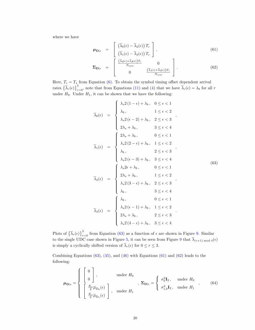
Plots of{λr(ε)
}3
r=0from Equation (63) as a function of ε are shown in Figure 9. Similar
to the single UDC case shown in Figure 5, it can be seen from Figure 9 that λ(r+1) mod 4(ε)
is simply a cyclically shifted version of λr(ε) for 0 ≤ r ≤ 3.
Combining Equations (63), (45), and (46) with Equations (61) and (62) leads to the
following:
µD|ε =
0
0
, under H0 Ks2 µD0
(ε)
Ks2 µD1
(ε)
, under H1
, ΣD|ε =
σ2b I2 , under H0
σ2s,bI2 , under H1
, (64)
20
²²
00 11 22 33 44
b b
2 s + b2 s + b
0(²) 0(²) 1(²) 1(²) 2(²) 2(²) 3(²) 3(²)
Figure 9. Plots of{λr(ε)
}3
r=0from Equation (63) as a function of ε for 0 ≤ ε < 4.
where µD0(ε) and µD1
(ε) are defined as
µD0(ε) ,
1− 2ε , 0 ≤ ε < 1
−1 , 1 ≤ ε < 2
−1 + 2 (ε− 2) , 2 ≤ ε < 3
1 , 3 ≤ ε < 4
,
µD1(ε) ,
1 , 0 ≤ ε < 1
1− 2 (ε− 1) , 1 ≤ ε < 2
−1 , 2 ≤ ε < 3
−1 + 2 (ε− 3) , 3 ≤ ε < 4
.
(65)
Using Equation (64) in Equation (60), it follows that under H0, we have
fD |H0(D) = fD0,D1 |H0
(D0, D1) =1
σ2b
φ
(D0
σb
)φ
(D1
σb
), (66)
whereas under H1, we have
fD |H1,ε(D | ε) = fD0,D1 |H1,ε(D0, D1 | ε) =1
σ2s,b
φ
(D0 − Ks
2 µD0(ε)
σs,b
)φ
(D1 − Ks
2 µD1(ε)
σs,b
).
(67)
Substituting Equations (67) and (65) into Equation (35), it can be shown that we have the
following after much algebraic manipulation:
fD0,D1 |H1(D0, D1) =
1
2
{1
Ks
[Φ
(D0 + Ks
2
σs,b
)− Φ
(D0 − Ks
2
σs,b
)]
× 1
2
[1
σs,bφ
(D1 + Ks
2
σs,b
)+
1
σs,bφ
(D1 − Ks
2
σs,b
)]
+1
Ks
[Φ
(D1 + Ks
2
σs,b
)− Φ
(D1 − Ks
2
σs,b
)]
×1
2
[1
σs,bφ
(D0 + Ks
2
σs,b
)+
1
σs,bφ
(D0 − Ks
2
σs,b
)]}. (68)
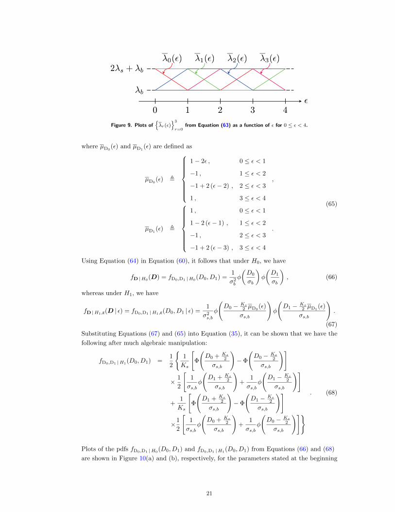
Plots of the pdfs fD0,D1 |H0(D0, D1) and fD0,D1 |H1
(D0, D1) from Equations (66) and (68)
are shown in Figure 10(a) and (b), respectively, for the parameters stated at the beginning
21

D0
D1
fD
0,D
1 |H
0(D
0 ,D1 )
−20 −15 −10 −5 0 5 10 15 20−20
−15
−10
−5
0
5
10
15
20
0.05
0.1
0.15
0.2
0.25
0.3
(a)
D0
D1
fD
0,D
1 |H
1(D
0 ,D1 )
−20 −15 −10 −5 0 5 10 15 20−20
−15
−10
−5
0
5
10
15
20
0
2
4
6
8
10
12
x 10−3
(b)
Figure 10. Dual UDC, single phase pdf plots: (a) fD0,D1 |H0(D0, D1) and (b) fD0,D1 |H1
(D0, D1). (Here,
Ks = 13.1072, Kb = 65.536, and Nsym = 255.)
of this section. As can be seen, fD0,D1 |H0(D0, D1) is concentrated near the origin, whereas
fD0,D1 |H1(D0, D1) is concentrated along an L∞ norm circle of radius Ks
2 [8].
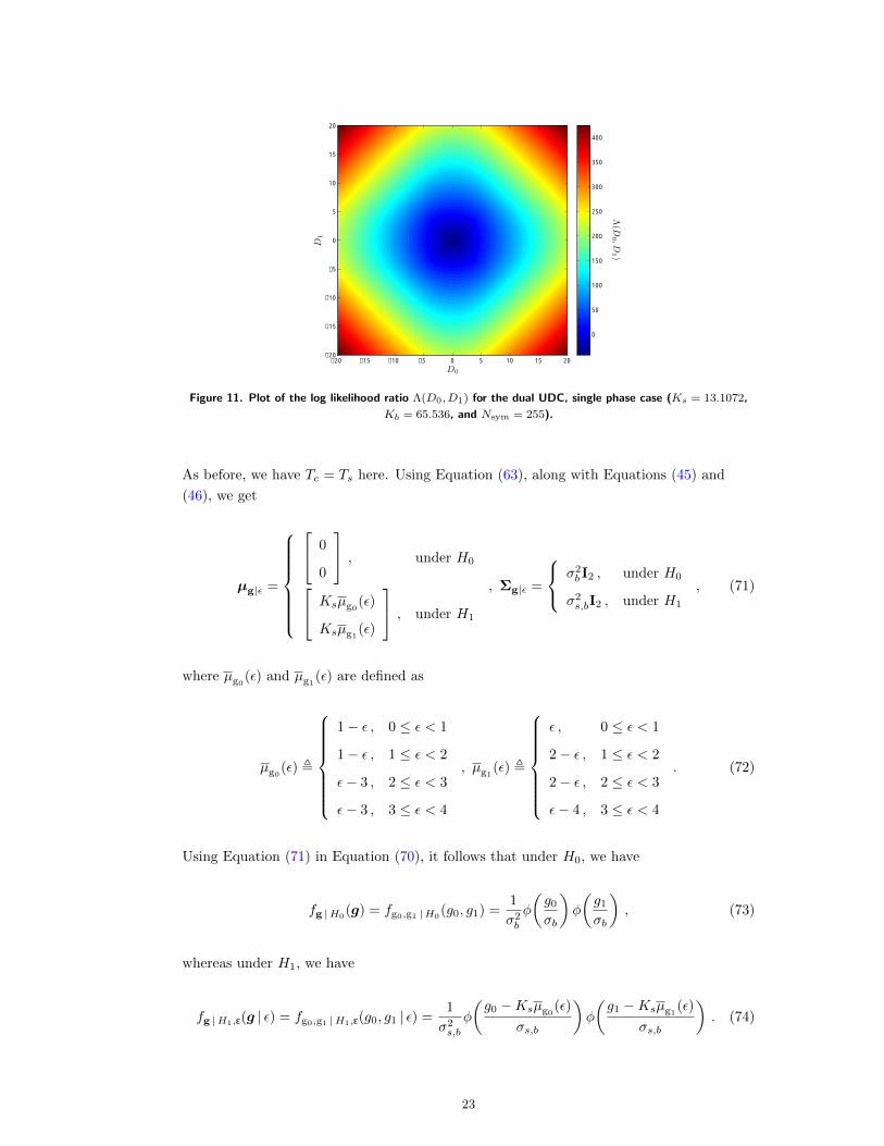
A plot of the log likelihood ratio Λ(D0, D1) given by Equations (33), (68), and (66) is
shown in Figure 11 for the above mentioned parameters. As can be seen, the behavior of
the log likelihood ratio is difficult to deduce and there does not appear to be a tractable
form for the decision regions RH0and RH1
from Equations (40) and (38), respectively, for
a given threshold value η.
From the view of the present hypothesis pdf fD0,D1 |H1(D0, D1) shown in Figure 10(b) as
well as that of the log likelihood ratio Λ(D0, D1) for small arguments given in Figure 11, it
appears as though an approximate log likelihood ratio decision based rule is as follows:
||D||∞ = max {|D0| , |D1|}H1
≷H0
η , (69)
where ||x||∞ denotes the L∞ norm of a vector x [8].
C. Single UDC, Dual Phase Case
Once again, we have G = 2, and so from Equations (30), (31), and (32), we have the
following:
g | ε ∼ N2
(µg|ε,Σg|ε
), (70)
where we have
µg|ε =
(λ0(ε)− λ2(ε)
)Tc +
(λ1(ε)− λ3(ε)
)Tc
−(λ0(ε)− λ2(ε)
)Tc +
(λ1(ε)− λ3(ε)
)Tc
,Σg|ε =
[(λ0(ε) + λ2(ε)
)Tc
Nspp+
(λ1(ε) + λ3(ε)
)Tc
Nspp
]I2 .
22
D0
D1
Λ(D
0 ,D1 )
−20 −15 −10 −5 0 5 10 15 20−20
−15
−10
−5
0
5
10
15
20
0
50
100
150
200
250
300
350
400
Figure 11. Plot of the log likelihood ratio Λ(D0, D1) for the dual UDC, single phase case (Ks = 13.1072,
Kb = 65.536, and Nsym = 255).
As before, we have Tc = Ts here. Using Equation (63), along with Equations (45) and
(46), we get
µg|ε =
0
0
, under H0 Ksµg0(ε)
Ksµg1(ε)
, under H1
, Σg|ε =
σ2b I2 , under H0
σ2s,bI2 , under H1
, (71)
where µg0(ε) and µg1
(ε) are defined as
µg0(ε) ,
1− ε , 0 ≤ ε < 1
1− ε , 1 ≤ ε < 2
ε− 3 , 2 ≤ ε < 3
ε− 3 , 3 ≤ ε < 4
, µg1(ε) ,
ε , 0 ≤ ε < 1
2− ε , 1 ≤ ε < 2
2− ε , 2 ≤ ε < 3
ε− 4 , 3 ≤ ε < 4
. (72)
Using Equation (71) in Equation (70), it follows that under H0, we have
fg |H0(g) = fg0,g1 |H0
(g0, g1) =1
σ2b
φ
(g0
σb
)φ
(g1
σb
), (73)
whereas under H1, we have
fg |H1,ε(g | ε) = fg0,g1 |H1,ε(g0, g1 | ε) =1
σ2s,b
φ
(g0 −Ksµg0
(ε)
σs,b
)φ
(g1 −Ksµg1
(ε)
σs,b
). (74)
23
g0
g 1
fg0,g
1 |H
0(g
0 ,g1 )
−20 −15 −10 −5 0 5 10 15 20−20
−15
−10
−5
0
5
10
15
20
0
0.01
0.02
0.03
0.04
0.05
0.06
0.07
(a)
g0
g 1
fg0,g
1 |H
1(g
0 ,g1 )
−20 −15 −10 −5 0 5 10 15 20−20
−15
−10
−5
0
5
10
15
20
0
0.5
1
1.5
2
2.5
3
3.5
4
x 10−3
(b)
Figure 12. Single UDC, dual phase pdf plots: (a) fg0,g1 |H0(g0, g1) and (b) fg0,g1 |H1
(g0, g1). (Here,
Ks = 13.1072, Kb = 65.536, and Nspp = 128.)
Substituting Equations (74) and (72) into Equation (35), it can be shown that we have the
following after much algebraic manipulation:
fg0,g1 |H1(g0, g1) =
1
2
1
Ks
√2
Φ
(g0+g1√
2
)+ Ks√
2
σs,b
− Φ
(g0+g1√
2
)− Ks√
2
σs,b
× 1
2
1
σs,bφ
(g0−g1√
2
)+ Ks√
2
σs,b
+1
σs,bφ
(g0−g1√
2
)− Ks√
2
σs,b
+
1
Ks
√2
Φ
(g0−g1√
2
)+ Ks√
2
σs,b
− Φ
(g0−g1√
2
)− Ks√
2
σs,b
× 1
2
1
σs,bφ
(g0+g1√
2
)+ Ks√
2
σs,b
+1
σs,bφ
(g0+g1√
2
)− Ks√
2
σs,b
.
(75)
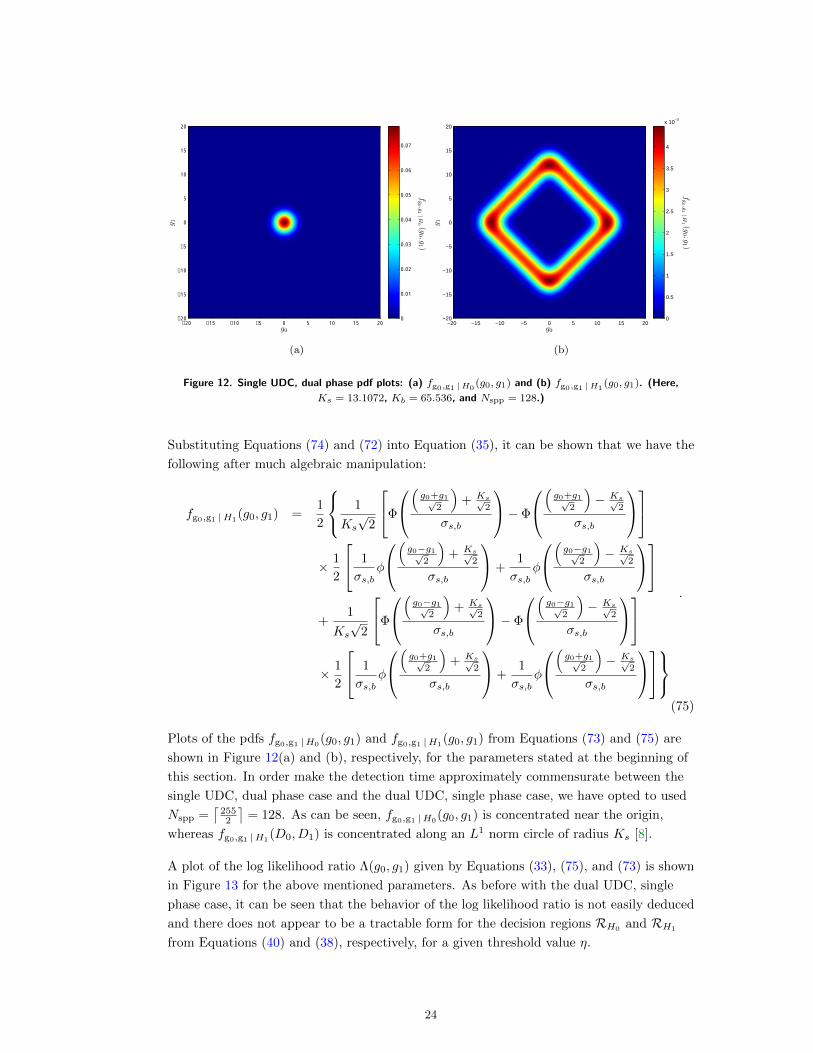
Plots of the pdfs fg0,g1 |H0(g0, g1) and fg0,g1 |H1
(g0, g1) from Equations (73) and (75) are
shown in Figure 12(a) and (b), respectively, for the parameters stated at the beginning of
this section. In order make the detection time approximately commensurate between the
single UDC, dual phase case and the dual UDC, single phase case, we have opted to used
Nspp =⌈
2552
⌉= 128. As can be seen, fg0,g1 |H0
(g0, g1) is concentrated near the origin,
whereas fg0,g1 |H1(D0, D1) is concentrated along an L1 norm circle of radius Ks [8].
A plot of the log likelihood ratio Λ(g0, g1) given by Equations (33), (75), and (73) is shown
in Figure 13 for the above mentioned parameters. As before with the dual UDC, single
phase case, it can be seen that the behavior of the log likelihood ratio is not easily deduced
and there does not appear to be a tractable form for the decision regions RH0and RH1
from Equations (40) and (38), respectively, for a given threshold value η.
24

g0
g 1
Λ(g
0 ,g1 )
−20 −15 −10 −5 0 5 10 15 20−20
−15
−10
−5
0
5
10
15
20
−20
0
20
40
60
80
100
Figure 13. Plot of the log likelihood ratio Λ(g0, g1) for the single UDC, dual phase case (Ks = 13.1072,
Kb = 65.536, and Nspp = 128).
From the view of the present hypothesis pdf fg0,g1 |H1(g0, g1) shown in Figure 12(b) as well
as that of the log likelihood ratio Λ(g0, g1) for small arguments given in Figure 13, it
appears as though an approximate log likelihood ratio decision based rule is as follows:
||g||1 = |g0|+ |g1|H1
≷H0
η , (76)
where ||x||1 denotes the L1 norm of a vector x [8].
VI. Worst Case Scenario Symbol Timing Offset Hypothesis Test Detection Analysis
Perhaps the main problem with assessing the performance of the unconditional
Neyman-Pearson hypothesis test is that determining the respective likelihood decision
regions RH0and RH1
from Equations (40) and (38) is often very difficult, as evidenced for
both the dual UDC, single phase system in Section V-B as well as the single UDC, dual
phase system in Section V-C. This, in turn, makes enforcing the false alarm probability
constraint and calculating the resulting probability of missed detection intractable.
One way to circumvent this problem is to derive the Neyman-Pearson hypothesis test
conditioned on a specific symbol timing offset value, as described in Section IV-A. For
example, one possible value to consider which is of practical significance is a worst case
scenario (WCS) symbol timing offset, in which the offset is exactly in between two timing
phases. From the definition of the chip interval Tc in Equation (6), it is clear that the
following symbol timing offsets represent WCS values:
εWCS =
(M + P
2G
)k +
(M + P
4G
), 0 ≤ k ≤ (2G)− 1 .
Without loss of generality, we can choose the first WCS offset, corresponding to k = 0. For
the case of M = P = 2 which we will focus on here, this then becomes εWCS = 1G .
25
From Equations (24), (25), (31), and (32), it is clear that the characteristics of the test
statistics for both the multiple UDC, single phase and single UDC, multiple phase systems
depend on the values of(λk(ε)− λG+k(ε)
)and
(λk(ε) + λG+k(ε)
)for 0 ≤ k ≤ G− 1.
Regardless of the value of ε, under H0, we have(λk(ε)− λG+k(ε)
)= 0 and(
λk(ε) + λG+k(ε))
= 2λb for all k. For the special case of εWCS = 1G , it can be show that
under H1, we have
λk(εWCS)− λG+k(εWCS) =
0 , k = 0
2λs , 1 ≤ k ≤ G− 1, (77)
λk(εWCS) + λG+k(εWCS) = 2 (λs + λb) = 2λs + 2λb ∀ 0 ≤ k ≤ G− 1 . (78)
Coupled with the fact that Tc = 2TsG here, we can use Equations (77) and (78) to simplify
the UDC test statistics and derive and assess the performance of the Neyman-Pearson
hypothesis test for a WCS symbol timing offset.
A. Multiple UDC, Single Phase Case
Combining Equations (77) and (78) with Equations (23), (24), (25), and (2), it can be
shown that we have
fD |H0(D) =
1
(2π)G2(det(ΣD|H0
)) 12
e− 1
2 (D−µD|H0)T
Σ−1D|H0
(D−µD|H0) , (79)
fD |H1,ε(D | εWCS) =1
(2π)G2(det(ΣD|H1,ε
)) 12
e− 1
2 (D−µD|H1,ε)T
Σ−1D|H1,ε
(D−µD|H1,ε) , (80)
where we have the following upon using Equations (45) and (46):
µD|H0= 0G×1 , ΣD|H0
= σ2b IG , (81)[
µD|H1,ε
]k
=
0 , k = 0
KsG , 1 ≤ k ≤ G− 1
, ΣD|H1,ε = σ2s,bIG . (82)
Upon using Equations (80) and (79) in Equations (41) and (42), we obtain the following
likelihood rule after much algebraic manipulation:
||D −DC ||2H1
≷H0
r20 , (83)
where DC is a G× 1 vector defined as
[DC ]k ,
0 , k = 0
− 4KbG , 1 ≤ k ≤ G− 1
, (84)
and r0 is a threshold value that is a function of the original threshold η from Equation
(42). Also, ||x|| denotes the Euclidean or L2 norm of a vector x [8]. Note that from
Equation (83), the decision rule boundary represents a G-dimensional hypersphere in RG
[8] with center at DC and radius r0. In addition, note that from Equation (84) that the
26
decision boundary center only depends on the mean background count Kb and the number
of UDCs G and does not depend on the number of symbols or the telemetry signal
parameters. From Equation (83), the decision regions are as follows:
RH0,{D : ||D −DC ||2 < r2
0
},RH1
,{D : ||D −DC ||2 > r2
0
}.
To enforce the false alarm probability constraint PFA = α, we use Equations (43), (79),
and (81) to get
PFA =
∫RH1
fD |H0(D) dD = 1−
∫RH0
fD |H0(D) dD = α .
From this, coupled with Equations (79) and (81), we find
1− α =
∫RH0
1
(2π)G2 σGb
e− 1
2σ2b
||D||2dD . (85)
Consider the change of variables x , 1σbD. Then, we have D = σbx and so dD = σGb dx.
In addition, we have ||D||2 = σ2b ||x||
2, and so Equation (85) becomes the following:
1− α =
∫Rx
1
(2π)G2
e−12 ||x||2 dx , (86)
where Rx is the region
Rx ,
{x : ||x− xC ||2 <
r20
σ2b
}, where xC ,
1
σbDC . (87)
Using the result from the Appendix given in Equation (A-1) with Equations (86) and (87)
leads to the following:
1− α = zNCχ2
(r20
σ2b
;G, ||xC ||2).
Inverting this relation to obtain the threshold r20 yields
r20 = σ2
bz−1NCχ2
(1− α;G, ||xC ||2
). (88)
To further simplify Equation (88), note that from Equations (87), (84), and (45) that we
have
||xC ||2 =1
σ2b
||DC ||2 =GNsym
4Kb·(−4Kb
G
)2
· (G− 1) = (4Kb)Nsym
(G− 1
G
).
Hence, Equation (88) simplifies to
r20 =
(4Kb
GNsym
)z−1NCχ2
(1− α;G, (4Kb)Nsym
(G− 1
G
)). (89)
Note that this relation provides for a way to determine the decision threshold r20 to satisfy
the false alarm probability constraint PFA = α. Assuming that r20 has already been
obtained as such, we can calculate the associated missed detection probability PMD.
27
To compute PMD, we use Equations (44), (80), and (82) to get
PMD =
∫RH0
fD |H1,ε(D | εWCS) dD =
∫RH0
1
(2π)G2 σGs,b
e− 1
2σ2s,b||D−µD|H1,ε
||2dD . (90)
As before, consider the change of variables x , 1σs,b
(D − µD|H1,ε
). Then, we have
D = σs,bx+ µD|H1,ε and so dD = σGs,bdx. Substituting this into Equation (90) leads to
the following:
PMD =
∫Rx
1
(2π)G2
e−12 ||x||2 dx , (91)
where Rx is the region
Rx ,
{x : ||x− xC ||2 <
r20
σ2s,b
}, where xC ,
1
σs,b
(DC − µD|H1,ε
). (92)
Exploiting the result from the Appendix given in Equation (A-1) with Equations (91) and
(92) leads to the following:
PMD = zNCχ2
(r20
σ2s,b
;G, ||xC ||2). (93)
To further simplify Equation (93), note that from Equations (92), (84), (82), and (46) that
we have
||xC ||2 =1
σ2s,b
∣∣∣∣∣∣DC − µD|H1,ε
∣∣∣∣∣∣2 =GNsym
Ks + 4Kb·(−4Kb
G− Ks
G
)2
· (G− 1) ,
= (Ks + 4Kb)Nsym
(G− 1
G
).
Hence, Equation (93) simplifies to
PMD = zNCχ2
r20[
Ks+4KbGNsym
] ;G, (Ks + 4Kb)Nsym
(G− 1
G
) . (94)
The relations given in Equations (89) and (94) provide a two-step process by which to
assess the performance of the Neyman-Pearson hypothesis test for a multiple UDC, single
phase system with a WCS symbol timing offset. First, the decision threshold parameter r20
is computed using Equation (89) to satisfy the false alarm probability constraint PFA = α
and then the missed detection probability is calculated as in Equation (94). An alternate,
simplified way to determine the performance of the hypothesis test is to define the
fictitious parameter β as β , (GNsym) r20. Then, we can assess the performance of the
Neyman-Pearson test as follows here:
1) Compute β = (4Kb)z−1NCχ2
(1− α;G, (4Kb)Nsym
(G− 1
G
)),
2) Calculate PMD = zNCχ2
(β
Ks + 4Kb;G, (Ks + 4Kb)Nsym
(G− 1
G
)).
(95)
28

100
101
102
10−10
10−9
10−8
10−7
10−6
10−5
10−4
10−3
10−2
10−1
100
Td (ms)
PM
D
G = 1
G = 2
G = 3
G = 4
G = 5
G = 6
G = 7
G = 8
G = 16
G = 32
G = 64
G = 128
G = 256
G = 512
G = 1024
Figure 14. Plot of the missed detection probability PMD given by Equation (95) as a function of the
detection time Td for the multiple UDC, single phase case for a WCS symbol timing offset (Ks = 13.1072,
Kb = 65.536, PFA = 10−3).
A plot of PMD given by Equation (95) as a function of the detection time Td = NsymTsym
is shown in Figure 14 for the parameters mentioned in Section V for various values of G.
As can be seen, the performance appears to asymptotically reach a limit as G→∞. This
represents a point of diminishing returns, as increasing G requires both an increase in
hardware (in terms of the number of UDCs required), as well as an increase in
computational complexity for implementing the hypothesis test specified by Equation (83).
For the suggested target of Nsym = 255 (see the beginning of Section V), we have
PMD ≈ 1.7628× 10⁻⁹ for G = 2, which is well below the possible maximum value of 10−6.
From this, we can conjecture that a dual UDC, single phase system would suffice for
uplink signal detection in this case.
B. Single UDC, Multiple Phase Case
As before, combining Equations (77) and (78) with Equations (30), (31), (32), and (2), it
can be shown that we have
fg |H0(g) =
1
(2π)G2(det(Σg|H0
)) 12
e− 1
2 (g−µg|H0)T
Σ−1g|H0
(D−µg|H0) , (96)
fg |H1,ε(g | εWCS) =1
(2π)G2(det(Σg|H1,ε
)) 12
e− 1
2 (g−µg|H1,ε)T
Σ−1g|H1,ε
(g−µg|H1,ε) , (97)
29
where we have the following upon using Equations (45) and (46):
µg|H0= 0G×1 , Σg|H0
= σ2b IG , (98)[
µg|H1,ε
]k
=Ks
G
G−1∑r=1
(−1)br−kG c , 0 ≤ k ≤ G− 1 , Σg|H1,ε = σ2
s,bIG . (99)
It can be shown that we have
G−1∑r=1
(−1)br−kG c =
G− 1 , k = 0
G− (2k − 1) , 1 ≤ k ≤ G− 1,
and so Equation (99) simplifies to
[µg|H1,ε
]k
=
Ks
(G−1G
), k = 0
Ks
(G−(2k−1)
G
), 1 ≤ k ≤ G− 1
, Σg|H1,ε = σ2s,bIG . (100)
Upon using Equations (97) and (96) in Equations (41) and (42), we obtain the following
likelihood rule after much algebraic manipulation:
||g − gC ||2H1
≷H0
r20 , (101)
where gC is a G× 1 vector defined as
[gC ]k ,
−4Kb
(G−1G
), k = 0
−4Kb
(G−(2k−1)
G
), 1 ≤ k ≤ G− 1
, (102)
and r0 is a threshold value that is a function of the original threshold η from Equation
(42). As for the multiple UDC, single phase case, note that from Equation (101), the
decision rule boundary represents a G-dimensional hypersphere in RG with center at gCand radius r0. In addition, note that from Equation (102) that the decision boundary
center only depends on the mean background count Kb and the number of UDCs G and
does not depend on the number of symbols or the telemetry signal parameters. From
Equation (101), the decision regions are as follows:
RH0 ,{g : ||g − gC ||
2< r2
0
},RH1 ,
{g : ||g − gC ||
2> r2
0
}.
To enforce the false alarm probability constraint PFA = α, we use Equations (43), (96),
and (98) to get
PFA =
∫RH1
fg |H0(g) dg = 1−
∫RH0
fg |H0(g) dg = α .
From this, coupled with Equations (96) and (98), we find
1− α =
∫RH0
1
(2π)G2 σGb
e− 1
2σ2b
||g||2dg . (103)
30
Consider the change of variables x , 1σbg. Then, we have g = σbx and so dg = σGb dx. In
addition, we have ||g||2 = σ2b ||x||
2, and so Equation (103) becomes the following:
1− α =
∫Rx
1
(2π)G2
e−12 ||x||2 dx , (104)
where Rx is the region
Rx ,
{x : ||x− xC ||2 <
r20
σ2b
}, where xC ,
1
σbgC . (105)
Using the result from the Appendix given in Equation (A-1) with Equations (104) and
(105) leads to the following:
1− α = zNCχ2
(r20
σ2b
;G, ||xC ||2).
Inverting this relation to obtain the threshold r20 yields
r20 = σ2
bz−1NCχ2
(1− α;G, ||xC ||2
). (106)
To further simplify Equation (106), note that from Equations (105), (102), and (45) that
we have
||xC ||2 =1
σ2b
||gC ||2
= (4Kb)Nspp
[(G− 1
G
)2
+
G−1∑k=1
(G− (2k − 1)
G
)2]. (107)
The expression given in Equation (107) can be simplified upon using the following
relations [7]:
G−1∑k=1
1 = G− 1 ,
G−1∑k=1
k =(G− 1)G
2,
G−1∑k=1
k2 =(G− 1)G (2G− 1)
6. (108)
Upon using Equation (108) in Equation (107), after some algebraic manipulation, we get
||xC ||2 = (4Kb)Nspp
(G2 − 1
3G
).
Hence, Equation (106) simplifies to
r20 =
(4Kb
Nspp
)z−1NCχ2
(1− α;G, (4Kb)Nspp
(G2 − 1
3G
)). (109)
Note that this relation provides for a way to determine the decision threshold r20 to satisfy
the false alarm probability constraint PFA = α. Assuming that r20 has already been
obtained as such, we can calculate the associated missed detection probability PMD.
To compute PMD, we use Equations (44), (97), and (100) to get
PMD =
∫RH0
fg |H1,ε(g | εWCS) dg =
∫RH0
1
(2π)G2 σGs,b
e− 1
2σ2s,b||g−µg|H1,ε
||2dg . (110)
31
As before, consider the change of variables x , 1σs,b
(g − µg|H1,ε
). Then, we have
g = σs,bx+ µg|H1,ε and so dg = σGs,bdx. Substituting this into Equation (110) leads to the
following:
PMD =
∫Rx
1
(2π)G2
e−12 ||x||2 dx , (111)
where Rx is the region
Rx ,
{x : ||x− xC ||2 <
r20
σ2s,b
}, where xC ,
1
σs,b
(gC − µg|H1,ε
). (112)
Exploiting the result from the Appendix given in Equation (A-1) with Equations (111)
and (112) leads to the following:
PMD = zNCχ2
(r20
σ2s,b
;G, ||xC ||2). (113)
To further simplify Equation (113), note that from Equations (112), (102), (100), (46), and
(108) that we can show that we have
||xC ||2 =1
σ2s,b
∣∣∣∣∣∣gC − µg|H1,ε
∣∣∣∣∣∣2 = (Ks + 4Kb)Nsym
(G2 − 1
3G
).
Hence, Equation (113) simplifies to
PMD = zNCχ2
r20[
Ks+4KbNspp
] ;G, (Ks + 4Kb)Nsym
(G2 − 1
3G
) . (114)
As with the multiple UDC, single phase system, the relations given in Equations (109) and
(114) provide a two-step process by which to assess the performance of the
Neyman-Pearson hypothesis test for a single UDC, multiple phase system with a WCS
symbol timing offset. First, the decision threshold parameter r20 is computed using
Equation (109) to satisfy the false alarm probability constraint PFA = α and then the
missed detection probability is calculated as in Equation (114). An alternate, simplified
way to determine the performance of the hypothesis test is to define the fictitious
parameter β as β , Nsppr20. Then, we can assess the performance of the Neyman-Pearson
test as follows here:
1) Compute β = (4Kb)z−1NCχ2
(1− α;G, (4Kb)Nspp
(G2 − 1
3G
)),
2) Calculate PMD = zNCχ2
(β
Ks + 4Kb;G, (Ks + 4Kb)Nspp
(G2 − 1
3G
)).
(115)
A plot of PMD given by Equation (115) as a function of the detection time
Td = NsppGTsym is shown in Figure 15 for the parameters mentioned in Section V for
various values of G. As can be seen, the performance appears to asymptotically reach a
limit as G→∞. This represents a point of diminishing returns, as increasing G requires
32

101
102
10−10
10−9
10−8
10−7
10−6
10−5
10−4
10−3
10−2
10−1
100
Td (ms)
PM
D
G = 1
G = 2
G = 3
G = 4
G = 5
G = 6
G = 7
G = 8
G = 16
G = 32
G = 64
G = 128
G = 256
G = 512
G = 1024
Figure 15. Plot of the missed detection probability PMD given by Equation (115) as a function of the
detection time Td for the single UDC, multiple phase case for a WCS symbol timing offset (Ks = 13.1072,
Kb = 65.536, PFA = 10−3).
both an increase in hardware (in terms of triggering and storing the count statistics for the
number of timing phases required), as well as an increase in computational complexity for
implementing the hypothesis test specified by Equation (101).
For the suggested target of Nsym = 255, corresponding to a detection time of
Td = 66.84672 ms (see Section I-C as well as the beginning of Section V), we have
PMD ≈ 4.9696× 10⁻⁴ for G = 2, which is well above the possible maximum value of 10−6.
From this, we can conjecture that a single UDC, dual phase system would not suffice for
uplink signal detection in this case.
VII. Advantages and Disadvantages Between the Multiple UDC, Single Phase and
Single UDC, Multiple Phase Detection Systems
As mentioned in Section VI-A and VI-B, for the suggested operating point considered here
(see the beginning of Section V), a dual UDC, single phase system would suffice for uplink
signal detection in the case of a WCS symbol timing offset, whereas a single UDC, dual
phase system would not. This brings to light some of the trade-offs associated with both
the multiple UDC, single phase and single UDC, multiple phase detection schemes.
For a fixed detection time Td, a multiple UDC, single phase system will exhibit greater
detection performance than a single UDC, multiple phase system. Intuitively, the reason
for this is that the former system has more information available to it to use for signal
detection than the latter one. To see this analytically, consider the conditional WCS
symbol timing offset detection results derived in Section VI. In the case where Td is fixed,
33

we have Nspp =Nsym
G (see Section I-C), and so the performance of the Neyman-Pearson
hypothesis test for a WCS symbol timing offset for the single UDC, multiple phase system
from Equation (115) becomes
1) Compute β = (4Kb)z−1NCχ2
(1− α;G, (4Kb)Nsym
(G− 1
G
)(G+ 1
3G
)),
2) Calculate PMD = zNCχ2
(β
Ks + 4Kb;G, (Ks + 4Kb)Nsym
(G− 1
G
)(G+ 1
3G
)).
(116)
Comparing Equation (116) with Equation (95), it is evident that the ratio of the
respective non-centrality parameters of the single UDC, multiple phase system to those of
the multiple UDC, single phase system is(G+13G
). For all G ∈ N, the factor
(G+13G
)is less
than unity and decreases monotonically with G. Asymptotically, we have(G+13G
)→ 1
3 as
G→∞. As(G+13G
)< 1 for all G ≥ 1, it follows that the respective non-centrality
parameters of the single UDC, multiple phase system are less than those of the multiple
UDC, single phase one. Since it can be shown that the missed detection probability PMD
decreases as the respective non-centrality parameters increase [4], it follows that the
multiple UDC, single phase system will always perform better than the corresponding
single UDC, multiple phase one. Furthermore, as(G+13G
)is monotonic decreasing with G,
it follows that the single UDC, multiple phase system will reach a point of diminishing
returns more rapidly than the corresponding multiple UDC, single phase system [4]. This
is evidenced upon comparing Figure 14 with Figure 15.
Despite the fact that a multiple UDC, single phase system outperforms a corresponding
single UDC, multiple phase type scheme for a fixed detection time, there are advantages to
using a single UDC, multiple phase system for signal detection. Specifically, if there is
some leeway with respect to increasing the detection time, then there are several benefits
to a single UDC, multiple phase type implementation. One such benefit is that while it is
difficult to increase the number of UDCs in a multiple UDC, single phase system in a
practical setting as it requires additional hardware, it is very simple to increase the number
of timing phases of a single UDC, multiple phase system, as the only changes required are
to trigger, store, and process the UDC test statistics at the different timing phases. At the
expense of an increase in detection time, the improvement in performance is dramatic and
is the result of both an increased detection time, as well as the number of timing phases.
For example, suppose that initially, G = 2 timing phases are used in a single UDC,
multiple phase system and that for some given detection time that the missed detection
probability is deemed excessively large. To improve the detection performance, we can, for
instance, trigger the UDC to accumulate additional statistics at 3 times finer resolution to
obtain an effective number of G = 6 timing phases. This only requires 6− 2 = 4 additional
UDC test statistics at different timing phases. In essence, from an initial detection time of
Td using G = 2 phases, we arrive at a final detection time of 3Td using G = 6 phases.
Thus, the benefits of an increased detection time are twofold: an inherent improvement in
performance as a result of the increased detection time as well as an additional
improvement due to the increased number of timing phases.
34
From a practical point of view, perhaps the most efficient manner in which to increase the
number of timing phases is to do so in powers of 2 until the missed detection probability
performance is deemed acceptable. Specifically, starting from G = 1 timing phase, we
double the timing resolution at each stage by accumulating additional UDC statistics as
required until the missed detection performance is below its target requirement. At the
k-th stage of such a detection scheme, the number of timing phases is G = 2k−1, while the
detection time is Td = 2k−1Td,0, where Td,0 denotes the nominal detection time per phase.
In summary, there are several pros and cons to using both of the proposed uplink signal
detection schemes. While a multiple UDC, single phase system offers improved
performance over a corresponding single UDC, multiple phase system for a fixed detection
time, it requires additional hardware and cannot easily accommodate increased timing
resolution. On the other hand, a single UDC, multiple phase system is amenable to
increased timing resolution, provided that there is sufficient leeway with regards to
increasing the detection time. Of course, with an implementation consisting of a fixed
number of multiple UDCs, improved performance could also be obtained by using multiple
timing phases instead of a single one. This would result in the most advantageous of all of
the schemes considered, as it would result in the most detection information for a given
detection time and number of UDCs.
VIII. Concluding Remarks
In this article, we focused on uplink signal detection for the DOT using the
Neyman-Pearson hypothesis test. Specifically, we considered this hypothesis test for two
different sets of test statistics: those from a multiple UDC, single phase system as well as
those from a single UDC, multiple phase type implementation. Conditioned on a WCS
symbol timing offset, we derived the performance of the Neyman-Pearson test for both sets
of statistics, and assessed the advantages and disadvantages of both detection schemes.
For specific test cases (namely the dual UDC, single phase and single UDC, dual phase
systems), we showed the problems inherent with deriving the performance of the bona fide
unconditional Neyman-Pearson test. In particular, we showed that determining the
decision regions based on the likelihood criterion was intractable for both cases. Future
work involves assessing the performance of a suboptimal Neyman-Pearson type test using
the conjectured decision regions given by Equations (69) and (76) for the dual UDC, single
phase and single UDC, dual phase schemes, respectively. In addition, it would be
worthwhile carrying out similar analysis for the more general multiple UDC, single phase
and single UDC, multiple phase systems.
References
[1] R. M. Gagliardi and S. Karp, Optical Communications, 2nd ed. New York, NY: John
Wiley & Sons, Inc., 1995.
35

[2] H. P. Hsu, Schaum’s Outline of Theory and Problems of Probability, Random
Variables, and Random Processes, ser. Schaum’s Outline. United States of America:
McGraw-Hill Companies, Inc., 1997.
[3] P. P. Vaidyanathan, Multirate Systems and Filter Banks. Englewood Cliffs, NJ:
Prentice Hall PTR, 1993.
[4] G. E. Corazza, Ed., Digital Satellite Communications. New York, NY: Springer
Science+Business Media, LLC, 2007.
[5] M. K. Simon, S. M. Hinedi, and W. C. Lindsey, Digital Communication Techniques:
Signal Design and Detection. Upper Saddle River, NJ: Prentice Hall PTR, 1995.
[6] K. J. Quirk, J. W. Gin, and M. Srinivasan, “Optical PPM Synchronization for Photon
Counting Receivers,” in Proc. Military Communications Conference (MILCOM 2008),
vol. 1, San Diego, California, USA, Nov. 17–19, 2008, pp. 1–7.
[7] I. S. Gradshteyn and I. M. Ryzhik, Table of Integrals, Series, and Products, 7th ed.,
A. Jeffrey and D. Zwillinger, Eds. Burlington, MA: Academic Press, 2007.
[8] B. C. Levy, Principles of Signal Detection and Parameter Estimation. New York, NY:
Springer Science+Business Media, LLC, 2008.
36

Appendix: Multivariate Gaussian Distribution Integral Over a Hypersphere
In this section, we prove the following result:∫x∈RG:||x−xC ||2<r2
1
(2π)G2
e−12 ||x||2 dx = zNCχ2
(r2;G, ||xC ||2
). (A-1)
Note that the integrand in Equation (A-1) is the pdf of a multivariate Gaussian or normal
distribution with NG(0, I), which is a generalization of the standard normal distribution to
the multivariate case [2]. Also, it should be noted that the region of integration in
Equation (A-1) is a hypersphere in RG [8]. As seen in Section VI, this integral arises when
deriving and assessing the performance of the Neyman-Pearson hypothesis test for uplink
signal detection, conditioned on a particular value of the symbol timing offset.
In deriving Equation (A-1), we will use the following result regarding the change of
variables of a multidimensional integral [7]. Suppose that u and v are two G× 1 vectors in
RG related by v = ϕ(u), where ϕ is an injective, differentiable function with continuous
partial derivatives [7]. Furthermore, suppose U and V are two open sets in RG such that
ϕ : U → V . Then, we have the following [7]:∫V
f(v) dv =
∫U
f(ϕ(u)) |det(J(ϕ(u)))| du , (A-2)
where J(ϕ(u)) is the G×G Jacobian matrix [7] of the transformation v = ϕ(u) whose
(k, `)-th element is given by
[J(ϕ(u))]k,` =∂ [v]k∂ [u]`
, 0 ≤ k ≤ G− 1 , 0 ≤ ` ≤ G− 1 .
To begin deriving Equation (A-1), consider the transformation y , U (x− xC), where U
is a unitary, Householder transformation matrix [3] given by
U , I− 2wwT , where w ,xC + ||xC || e0
||xC + ||xC || e0||, (A-3)
where e0 denotes the 0th unit vector [3] which is unity in the 0th component and zero
otherwise. (More generally, ek denotes the k-th unit vector [3] which is unity in the k-th
component and zero otherwise.) As U is a real unitary matrix, we have UTU = UUT = I
[3], and so x = UTy + xC = UT (y − yC), where yC , −UxC . From this relation, it is
clear that the Jacobian matrix is J(ϕ(y)) = UT , and so |det(J(ϕ(y)))| = 1 as U is unitary
[3]. Letting I denote the left hand side of Equation (A-1) and appealing to Equation
(A-2), we get
I ,∫x∈RG:||x−xC ||2<r2
1
(2π)G2
e−12 ||x||2 dx =
∫y∈RG:||y||2<r2
1
(2π)G2
e−12 ||y−yC ||2 dy . (A-4)
To simplify Equation (A-4), note that the vector yC has all zeros in it except for the 0th
component. In order to show this, recall that yC = −UxC and so from Equation (A-3) we
37

have
yC = −xC + 2(wTxC
)w = −xC +
2[||xC ||2 + ||xC || [xC ]0
]||xC + ||xC || e0||
w ,
= −xC +2[||xC ||2 + ||xC || [xC ]0
]||xC + ||xC || e0||2
[xC + ||xC || e0] ,
= −xC +2[||xC ||2 + ||xC || [xC ]0
]2[||xC ||2 + ||xC || [xC ]0
] [xC + ||xC || e0] = −xC + xC + ||xC || e0 .
Thus, we have yC = ||xC || e0, and so indeed the only nonzero component of yC is its 0th
component. Substituting this into Equation (A-4) and defining yk , [y]k for all
0 ≤ k ≤ G− 1 for notational convenience leads to
I =
∫y∈RG:||y||2<r2
1
(2π)G2
e−12 ||y−||xC ||e0||2 dy ,
=
∫y∈RG:||y||2<r2
1
(2π)G2
e−12 (||y||2−2||xC ||y0+||xC ||2) dy . (A-5)
To evaluate Equation (A-5), consider the following hyperspherical coordinate system [8]
transformation:
y0 = ρ cos(φ0) ,
y1 = ρ sin(φ0) cos(φ1) ,
y2 = ρ sin(φ0) sin(φ1) cos(φ2) ,
...
yG−2 = ρ sin(φ0) sin(φ1) · · · sin(φG−3) cos(φG−2) ,
yG−1 = ρ sin(φ0) sin(φ1) · · · sin(φG−3) sin(φG−2) .
Here, ρ denotes the radial coordinate, while φ0, φ1, . . . , φG−2 represent the angular
coordinates. In a more compact form, we have
yk =
ρ
[k−1∏`=0
sin(φ`)
]cos(φk) , 0 ≤ k ≤ G− 2
ρ
[k−1∏`=0
sin(φ`)
], k = G− 1
, (A-6)
where all empty products are assumed to be equal to unity here. With the transformation
given in Equation (A-6), it can be shown that the differential dy satisfies [8]
dy = ρG−1 sinG−2(φ0) sinG−3(φ1) · · · sin2(φG−4) sin(φG−3) dρ dφ0 dφ1 · · · dφG−2 ,
which can be expressed more compactly as
dy = ρG−1
[G−2∏`=0
sinG−2−`(φ`)
]dρ
(G−2∏`=0
dφ`
). (A-7)
38

Using Equations (A-6) and (A-7) in Equation (A-5) and noting that ||y||2 < r2 corresponds
to the region 0 ≤ ρ < r, 0 ≤ φ0 < π, 0 ≤ φ1 < π, . . . , 0 ≤ φG−3 < π, 0 ≤ φG−2 < 2π leads to
I =
∫ r
ρ=0
∫ π
φ0=0
∫ π
φ1=0
· · ·∫ π
φG−3=0
∫ 2π
φG−2=0
1
(2π)G2
e−12 (ρ2−2||xC ||ρ cos(φ0)+||xC ||2)
× ρG−1
[G−2∏`=0
sinG−2−`(φ`)
]dρ
(G−2∏`=0
dφ`
).
This can be simplified to
I =
∫ r
ρ=0
ρG−1
(2π)G2
e−12 (ρ2+||xC ||2)
∫ π
φ0=0
e||xC ||ρ cos(φ0) sinG−2(φ0)
×
[G−3∏`=1
∫ π
0
sinG−2−`(φ`) dφ`
](∫ 2π
0
1 dφG−2
)dφ0 dρ ,
which in turn can be simplified to the following:
I = 2π
(G−3∏`=1
∫ π
0
sin` x dx
)[∫ r
0
ρG−1
(2π)G2
e−12 (ρ2+||xC ||2)
(∫ π
0
e||xC ||ρ cosφ sinG−2φdφ
)dρ
].
(A-8)
In order to continue further with the simplification of I, we will first use the following
result from [7, pg. 397]:∫ π
0
sinν−1x cos (ax) dx =π cos
(aπ2
)2ν−1νB
(ν+a+1
2 , ν−a+12
) , Re [ν] > 0 ,
where B(x, y) is the beta function [7]. Setting ν = `+ 1 and a = 0 yields∫ π
0
sin` x dx =π
2` (`+ 1)B(`2 + 1, `2 + 1
) . (A-9)
But from [7, pg. 909], we have B(x, y) = Γ(x)Γ(y)Γ(x+y) , where Γ(x) is the gamma function [7],
and so B(x, x) = (Γ(x))2
Γ(2x) . By the doubling formula for the gamma function [7, pg. 896], we
have Γ(2x) = 22x−1√π
Γ(x) Γ(x+ 1
2
), and thus B(x, x) =
√π Γ(x)
22x−1Γ(x+ 12 )
. Substituting this into
Equation (A-9) leads to ∫ π
0
sin` x dx =
√π Γ(`+1
2 + 1)(
`+12
)Γ(`2 + 1
) .Now, as Γ(x+ 1) = xΓ(x) [7, pg. 895], we have∫ π
0
sin` x dx =√π
Γ(`−1
2 + 1)
Γ(`2 + 1
) , (A-10)
and henceG−3∏`=1
∫ π
0
sin` x dx = π(G2 − 32 ) · Γ(1)
Γ(G2 −
12
) =π(G2 − 3
2 )
Γ(G2 −
12
) . (A-11)
Here, Equation (A-11) follows from the fact that the gamma function terms in Equation
(A-10) form a telescoping product [7] and the fact that Γ(1) = 1 [7, pg. 897].
39
Returning to Equation (A-8), it follows that substituting Equation (A-11) yields the
following:
I =2π(G2 − 1
2 )
Γ(G2 −
12
) ∫ r
0
ρG−1
(2π)G2
e−12 (ρ2+||xC ||2)
(∫ π
0
e||xC ||ρ cosφ sinG−2φdφ
)dρ . (A-12)
To simplify the inner integral, note that from [7, pg. 491] that we have∫ π
0
e±β cos x sin2νx dx =√π
(2
β
)νΓ
(ν +
1
2
)Iν(β) , Re [ν] > −1
2,
where Iν(x) is the modified Bessel function of the first kind of order ν [7]. Setting
β = ||xC || ρ and ν = G2 − 1 yields
∫ π
0
e||xC ||ρ cosφ sinG−2φdφ =√π
(2
||xC || ρ
)G2 −1
Γ
(G
2− 1
2
)IG
2 −1(||xC || ρ) .
Substituting this result into Equation (A-12) leads to
I = ||xC ||−G2 +1
∫ r
0
ρG2 e−
12 (ρ2+||xC ||2)IG
2 −1(||xC || ρ) dρ . (A-13)
Let u , ρ2, so that ρ =√u and thus dρ = 1
2u− 1
2 du. Then, with this change of variables
applied to Equation (A-13), we get
I =
∫ r2
0
1
2e−
12 (u+||xC ||2)
(u
||xC ||2
)G4 − 1
2
IG2 −1
(√||xC ||2 u
)︸ ︷︷ ︸
fNCχ2(u;G,||xC ||2)
du ,
where fNCχ2
(u;G, ||xC ||2
)is the pdf of a noncentral chi-square distribution evaluated at
u with G degrees of freedom and non-centrality parameter ||xC ||2 [4]. As the cdf of any
distribution is simply the integral of the associated pdf from −∞ to the point of interest
[2], and since the region of support of a noncentral chi-square random variable is [0,∞) [4],
we have
I = zNCχ2
(r2;G, ||xC ||2
), (A-14)
and so Equations (A-14) and (A-4) imply Equation (A-1). This completes the proof.
JPL CL#12-1560
40