Deep Neural Networks for YouTube Recommendations

Paul Covington, Jay Adams, Emre SarginGoogle

Mountain View, CA{pcovington, jka, msargin}@google.com

ABSTRACTYouTube represents one of the largest scale and most sophis-ticated industrial recommendation systems in existence. Inthis paper, we describe the system at a high level and fo-cus on the dramatic performance improvements brought bydeep learning. The paper is split according to the classictwo-stage information retrieval dichotomy: first, we detail adeep candidate generation model and then describe a sepa-rate deep ranking model. We also provide practical lessonsand insights derived from designing, iterating and maintain-ing a massive recommendation system with enormous user-facing impact.

Keywordsrecommender system; deep learning; scalability

1. INTRODUCTIONYouTube is the world’s largest platform for creating, shar-

ing and discovering video content. YouTube recommenda-tions are responsible for helping more than a billion usersdiscover personalized content from an ever-growing corpusof videos. In this paper we will focus on the immense im-pact deep learning has recently had on the YouTube videorecommendations system. Figure 1 illustrates the recom-mendations on the YouTube mobile app home.

Recommending YouTube videos is extremely challengingfrom three major perspectives:

• Scale: Many existing recommendation algorithms provento work well on small problems fail to operate on ourscale. Highly specialized distributed learning algorithmsand efficient serving systems are essential for handlingYouTube’s massive user base and corpus.

• Freshness: YouTube has a very dynamic corpus withmany hours of video are uploaded per second. Therecommendation system should be responsive enoughto model newly uploaded content as well as the lat-est actions taken by the user. Balancing new content

Permission to make digital or hard copies of part or all of this work for personal orclassroom use is granted without fee provided that copies are not made or distributedfor profit or commercial advantage and that copies bear this notice and the full citationon the first page. Copyrights for third-party components of this work must be honored.RecSys ’16 September 15-19, 2016, Boston , MA, USAc© 2016 Copyright held by the owner/author(s).

ACM ISBN 978-1-4503-4035-9/16/09.

DOI: http://dx.doi.org/10.1145/2959100.2959190

Figure 1: Recommendations displayed on YouTubemobile app home.

with well-established videos can be understood froman exploration/exploitation perspective.

• Noise: Historical user behavior on YouTube is inher-ently difficult to predict due to sparsity and a vari-ety of unobservable external factors. We rarely ob-tain the ground truth of user satisfaction and insteadmodel noisy implicit feedback signals. Furthermore,metadata associated with content is poorly structuredwithout a well defined ontology. Our algorithms needto be robust to these particular characteristics of ourtraining data.

In conjugation with other product areas across Google,YouTube has undergone a fundamental paradigm shift to-wards using deep learning as a general-purpose solution fornearly all learning problems. Our system is built on GoogleBrain [4] which was recently open sourced as TensorFlow [1].TensorFlow provides a flexible framework for experimentingwith various deep neural network architectures using large-scale distributed training. Our models learn approximatelyone billion parameters and are trained on hundreds of bil-lions of examples.

In contrast to vast amount of research in matrix factoriza-

191

tion methods [19], there is relatively little work using deepneural networks for recommendation systems. Neural net-works are used for recommending news in [17], citations in[8] and review ratings in [20]. Collaborative filtering is for-mulated as a deep neural network in [22] and autoencodersin [18]. Elkahky et al. used deep learning for cross domainuser modeling [5]. In a content-based setting, Burges et al.used deep neural networks for music recommendation [21].

The paper is organized as follows: A brief system overviewis presented in Section 2. Section 3 describes the candidategeneration model in more detail, including how it is trainedand used to serve recommendations. Experimental resultswill show how the model benefits from deep layers of hiddenunits and additional heterogeneous signals. Section 4 detailsthe ranking model, including how classic logistic regressionis modified to train a model predicting expected watch time(rather than click probability). Experimental results willshow that hidden layer depth is helpful as well in this situa-tion. Finally, Section 5 presents our conclusions and lessonslearned.

2. SYSTEM OVERVIEWThe overall structure of our recommendation system is il-

lustrated in Figure 2. The system is comprised of two neuralnetworks: one for candidate generation and one for ranking.

The candidate generation network takes events from theuser’s YouTube activity history as input and retrieves asmall subset (hundreds) of videos from a large corpus. Thesecandidates are intended to be generally relevant to the userwith high precision. The candidate generation network onlyprovides broad personalization via collaborative filtering.The similarity between users is expressed in terms of coarsefeatures such as IDs of video watches, search query tokensand demographics.

Presenting a few “best” recommendations in a list requiresa fine-level representation to distinguish relative importanceamong candidates with high recall. The ranking networkaccomplishes this task by assigning a score to each videoaccording to a desired objective function using a rich set offeatures describing the video and user. The highest scoringvideos are presented to the user, ranked by their score.

The two-stage approach to recommendation allows us tomake recommendations from a very large corpus (millions)of videos while still being certain that the small number ofvideos appearing on the device are personalized and engag-ing for the user. Furthermore, this design enables blendingcandidates generated by other sources, such as those de-scribed in an earlier work [3].

During development, we make extensive use of offline met-rics (precision, recall, ranking loss, etc.) to guide iterativeimprovements to our system. However for the final deter-mination of the effectiveness of an algorithm or model, werely on A/B testing via live experiments. In a live experi-ment, we can measure subtle changes in click-through rate,watch time, and many other metrics that measure user en-gagement. This is important because live A/B results arenot always correlated with offline experiments.

3. CANDIDATE GENERATIONDuring candidate generation, the enormous YouTube cor-

pus is winnowed down to hundreds of videos that may berelevant to the user. The predecessor to the recommender

candidate ranking

user history and context

generationmillions hundreds dozens

videocorpus

other candidate sourcesvideo

features

Figure 2: Recommendation system architecturedemonstrating the “funnel” where candidate videosare retrieved and ranked before presenting only afew to the user.

described here was a matrix factorization approach trainedunder rank loss [23]. Early iterations of our neural networkmodel mimicked this factorization behavior with shallownetworks that only embedded the user’s previous watches.From this perspective, our approach can be viewed as a non-linear generalization of factorization techniques.

3.1 Recommendation as ClassificationWe pose recommendation as extreme multiclass classifica-

tion where the prediction problem becomes accurately clas-sifying a specific video watch wt at time t among millionsof videos i (classes) from a corpus V based on a user U andcontext C,

P (wt = i|U,C) =eviu∑

j∈V evju

where u ∈ RN represents a high-dimensional “embedding” ofthe user, context pair and the vj ∈ RN represent embeddingsof each candidate video. In this setting, an embedding issimply a mapping of sparse entities (individual videos, usersetc.) into a dense vector in RN . The task of the deep neuralnetwork is to learn user embeddings u as a function of theuser’s history and context that are useful for discriminatingamong videos with a softmax classifier.

Although explicit feedback mechanisms exist on YouTube(thumbs up/down, in-product surveys, etc.) we use the im-plicit feedback [16] of watches to train the model, where auser completing a video is a positive example. This choice isbased on the orders of magnitude more implicit user historyavailable, allowing us to produce recommendations deep inthe tail where explicit feedback is extremely sparse.

Efficient Extreme MulticlassTo efficiently train such a model with millions of classes, werely on a technique to sample negative classes from the back-ground distribution (“candidate sampling”) and then correctfor this sampling via importance weighting [10]. For each ex-ample the cross-entropy loss is minimized for the true labeland the sampled negative classes. In practice several thou-sand negatives are sampled, corresponding to more than 100times speedup over traditional softmax. A popular alterna-tive approach is hierarchical softmax [15], but we weren’t

192

able to achieve comparable accuracy. In hierarchical soft-max, traversing each node in the tree involves discriminat-ing between sets of classes that are often unrelated, makingthe classification problem much more difficult and degradingperformance.

At serving time we need to compute the most likely Nclasses (videos) in order to choose the top N to presentto the user. Scoring millions of items under a strict serv-ing latency of tens of milliseconds requires an approximatescoring scheme sublinear in the number of classes. Previoussystems at YouTube relied on hashing [24] and the classi-fier described here uses a similar approach. Since calibratedlikelihoods from the softmax output layer are not neededat serving time, the scoring problem reduces to a nearestneighbor search in the dot product space for which generalpurpose libraries can be used [12]. We found that A/B re-sults were not particularly sensitive to the choice of nearestneighbor search algorithm.

3.2 Model ArchitectureInspired by continuous bag of words language models [14],

we learn high dimensional embeddings for each video in afixed vocabulary and feed these embeddings into a feedfor-ward neural network. A user’s watch history is representedby a variable-length sequence of sparse video IDs which ismapped to a dense vector representation via the embed-dings. The network requires fixed-sized dense inputs andsimply averaging the embeddings performed best among sev-eral strategies (sum, component-wise max, etc.). Impor-tantly, the embeddings are learned jointly with all othermodel parameters through normal gradient descent back-propagation updates. Features are concatenated into a widefirst layer, followed by several layers of fully connected Rec-tified Linear Units (ReLU) [6]. Figure 3 shows the generalnetwork architecture with additional non-video watch fea-tures described below.

3.3 Heterogeneous SignalsA key advantage of using deep neural networks as a gener-

alization of matrix factorization is that arbitrary continuousand categorical features can be easily added to the model.Search history is treated similarly to watch history - eachquery is tokenized into unigrams and bigrams and each to-ken is embedded. Once averaged, the user’s tokenized, em-bedded queries represent a summarized dense search history.Demographic features are important for providing priors sothat the recommendations behave reasonably for new users.The user’s geographic region and device are embedded andconcatenated. Simple binary and continuous features suchas the user’s gender, logged-in state and age are input di-rectly into the network as real values normalized to [0, 1].

“Example Age” FeatureMany hours worth of videos are uploaded each second toYouTube. Recommending this recently uploaded (“fresh”)content is extremely important for YouTube as a product.We consistently observe that users prefer fresh content, thoughnot at the expense of relevance. In addition to the first-ordereffect of simply recommending new videos that users wantto watch, there is a critical secondary phenomenon of boot-strapping and propagating viral content [11].

Machine learning systems often exhibit an implicit biastowards the past because they are trained to predict future

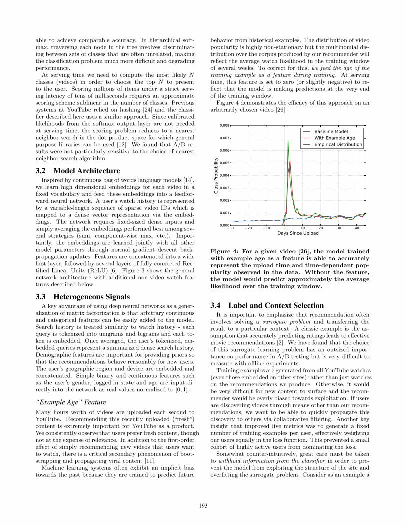
behavior from historical examples. The distribution of videopopularity is highly non-stationary but the multinomial dis-tribution over the corpus produced by our recommender willreflect the average watch likelihood in the training windowof several weeks. To correct for this, we feed the age of thetraining example as a feature during training. At servingtime, this feature is set to zero (or slightly negative) to re-flect that the model is making predictions at the very endof the training window.

Figure 4 demonstrates the efficacy of this approach on anarbitrarily chosen video [26].

−30 −20 −10 0 10 20 30 40

Days Since Upload

0.000

0.001

0.002

0.003

0.004

0.005

0.006

0.007

0.008

Cla

ss P

robabilit

y

Baseline Model

With Example Age

Empirical Distribution

Figure 4: For a given video [26], the model trainedwith example age as a feature is able to accuratelyrepresent the upload time and time-dependant pop-ularity observed in the data. Without the feature,the model would predict approximately the averagelikelihood over the training window.

3.4 Label and Context SelectionIt is important to emphasize that recommendation often

involves solving a surrogate problem and transferring theresult to a particular context. A classic example is the as-sumption that accurately predicting ratings leads to effectivemovie recommendations [2]. We have found that the choiceof this surrogate learning problem has an outsized impor-tance on performance in A/B testing but is very difficult tomeasure with offline experiments.

Training examples are generated from all YouTube watches(even those embedded on other sites) rather than just watcheson the recommendations we produce. Otherwise, it wouldbe very difficult for new content to surface and the recom-mender would be overly biased towards exploitation. If usersare discovering videos through means other than our recom-mendations, we want to be able to quickly propagate thisdiscovery to others via collaborative filtering. Another keyinsight that improved live metrics was to generate a fixednumber of training examples per user, effectively weightingour users equally in the loss function. This prevented a smallcohort of highly active users from dominating the loss.

Somewhat counter-intuitively, great care must be takento withhold information from the classifier in order to pre-vent the model from exploiting the structure of the site andoverfitting the surrogate problem. Consider as an example a

193

user vector

video vectors

averageaverage

watch vector search vector

embedded search tokensembedded video watches

example agegender

geographicembedding

trainingserving

ReLU

ReLU

ReLU

approx. top N

softmax

class probabilities

nearest neighborindex

Figure 3: Deep candidate generation model architecture showing embedded sparse features concatenated withdense features. Embeddings are averaged before concatenation to transform variable sized bags of sparse IDsinto fixed-width vectors suitable for input to the hidden layers. All hidden layers are fully connected. Intraining, a cross-entropy loss is minimized with gradient descent on the output of the sampled softmax.At serving, an approximate nearest neighbor lookup is performed to generate hundreds of candidate videorecommendations.

case in which the user has just issued a search query for“tay-lor swift”. Since our problem is posed as predicting the nextwatched video, a classifier given this information will predictthat the most likely videos to be watched are those whichappear on the corresponding search results page for “tay-lor swift”. Unsurpisingly, reproducing the user’s last searchpage as homepage recommendations performs very poorly.By discarding sequence information and representing searchqueries with an unordered bag of tokens, the classifier is nolonger directly aware of the origin of the label.

Natural consumption patterns of videos typically lead tovery asymmetric co-watch probabilities. Episodic series areusually watched sequentially and users often discover artistsin a genre beginning with the most broadly popular beforefocusing on smaller niches. We therefore found much betterperformance predicting the user’s next watch, rather thanpredicting a randomly held-out watch (Figure 5). Many col-laborative filtering systems implicitly choose the labels andcontext by holding out a random item and predicting it fromother items in the user’s history (5a). This leaks future infor-

mation and ignores any asymmetric consumption patterns.In contrast, we “rollback” a user’s history by choosing a ran-dom watch and only input actions the user took before theheld-out label watch (5b).

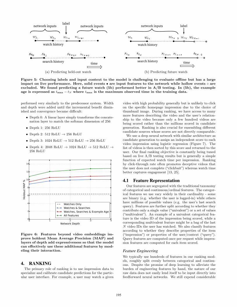
3.5 Experiments with Features and DepthAdding features and depth significantly improves preci-

sion on holdout data as shown in Figure 6. In these exper-iments, a vocabulary of 1M videos and 1M search tokenswere embedded with 256 floats each in a maximum bag sizeof 50 recent watches and 50 recent searches. The softmaxlayer outputs a multinomial distribution over the same 1Mvideo classes with a dimension of 256 (which can be thoughtof as a separate output video embedding). These modelswere trained until convergence over all YouTube users, corre-sponding to several epochs over the data. Network structurefollowed a common “tower” pattern in which the bottom ofthe network is widest and each successive hidden layer halvesthe number of units (similar to Figure 3). The depth zeronetwork is effectively a linear factorization scheme which

194

watch history

search history time

labelnetwork inputsnetwork inputs

(a) Predicting held-out watch

network inputs label

watch history

search history time

(b) Predicting future watch

Figure 5: Choosing labels and input context to the model is challenging to evaluate offline but has a largeimpact on live performance. Here, solid events • are input features to the network while hollow events ◦ areexcluded. We found predicting a future watch (5b) performed better in A/B testing. In (5b), the exampleage is expressed as tmax − tN where tmax is the maximum observed time in the training data.

performed very similarly to the predecessor system. Widthand depth were added until the incremental benefit dimin-ished and convergence became difficult:

• Depth 0: A linear layer simply transforms the concate-nation layer to match the softmax dimension of 256

• Depth 1: 256 ReLU

• Depth 2: 512 ReLU → 256 ReLU

• Depth 3: 1024 ReLU → 512 ReLU → 256 ReLU

• Depth 4: 2048 ReLU → 1024 ReLU → 512 ReLU →256 ReLU

0 1 2 3 4

Network Depth

0

2

4

6

8

10

12

14

Hold

out

MA

P %

Watches Only

Watches & Searches

Watches, Searches & Example Age

All Features

Figure 6: Features beyond video embeddings im-prove holdout Mean Average Precision (MAP) andlayers of depth add expressiveness so that the modelcan effectively use these additional features by mod-eling their interaction.

4. RANKINGThe primary role of ranking is to use impression data to

specialize and calibrate candidate predictions for the partic-ular user interface. For example, a user may watch a given

video with high probability generally but is unlikely to clickon the specific homepage impression due to the choice ofthumbnail image. During ranking, we have access to manymore features describing the video and the user’s relation-ship to the video because only a few hundred videos arebeing scored rather than the millions scored in candidategeneration. Ranking is also crucial for ensembling differentcandidate sources whose scores are not directly comparable.

We use a deep neural network with similar architecture ascandidate generation to assign an independent score to eachvideo impression using logistic regression (Figure 7). Thelist of videos is then sorted by this score and returned to theuser. Our final ranking objective is constantly being tunedbased on live A/B testing results but is generally a simplefunction of expected watch time per impression. Rankingby click-through rate often promotes deceptive videos thatthe user does not complete (“clickbait”) whereas watch timebetter captures engagement [13, 25].

4.1 Feature RepresentationOur features are segregated with the traditional taxonomy

of categorical and continuous/ordinal features. The categor-ical features we use vary widely in their cardinality - someare binary (e.g. whether the user is logged-in) while othershave millions of possible values (e.g. the user’s last searchquery). Features are further split according to whether theycontribute only a single value (“univalent”) or a set of values(“multivalent”). An example of a univalent categorical fea-ture is the video ID of the impression being scored, while acorresponding multivalent feature might be a bag of the lastN video IDs the user has watched. We also classify featuresaccording to whether they describe properties of the item(“impression”) or properties of the user/context (“query”).Query features are computed once per request while impres-sion features are computed for each item scored.

Feature EngineeringWe typically use hundreds of features in our ranking mod-els, roughly split evenly between categorical and continu-ous. Despite the promise of deep learning to alleviate theburden of engineering features by hand, the nature of ourraw data does not easily lend itself to be input directly intofeedforward neural networks. We still expend considerable

195

logistic

languageaverage

normalizenormalize

ReLU

ReLU

ReLU

serving training

embedding

video languageuser language

videoembedding

watched video IDsimpression video IDtime sincelast watch

# previousimpressions

weighted

Figure 7: Deep ranking network architecture depicting embedded categorical features (both univalent andmultivalent) with shared embeddings and powers of normalized continuous features. All layers are fullyconnected. In practice, hundreds of features are fed into the network.

engineering resources transforming user and video data intouseful features. The main challenge is in representing a tem-poral sequence of user actions and how these actions relateto the video impression being scored.

We observe that the most important signals are those thatdescribe a user’s previous interaction with the item itself andother similar items, matching others’ experience in rankingads [7]. As an example, consider the user’s past history withthe channel that uploaded the video being scored - how manyvideos has the user watched from this channel? When wasthe last time the user watched a video on this topic? Thesecontinuous features describing past user actions on relateditems are particularly powerful because they generalize wellacross disparate items. We have also found it crucial topropagate information from candidate generation into rank-ing in the form of features, e.g. which sources nominatedthis video candidate? What scores did they assign?

Features describing the frequency of past video impres-sions are also critical for introducing “churn” in recommen-dations (successive requests do not return identical lists). Ifa user was recently recommended a video but did not watchit then the model will naturally demote this impression onthe next page load. Serving up-to-the-second impressionand watch history is an engineering feat onto itself outsidethe scope of this paper, but is vital for producing responsiverecommendations.

Embedding Categorical FeaturesSimilar to candidate generation, we use embeddings to mapsparse categorical features to dense representations suitablefor neural networks. Each unique ID space (“vocabulary”)

has a separate learned embedding with dimension that in-creases approximately proportional to the logarithm of thenumber of unique values. These vocabularies are simplelook-up tables built by passing over the data once beforetraining. Very large cardinality ID spaces (e.g. video IDsor search query terms) are truncated by including only thetop N after sorting based on their frequency in clicked im-pressions. Out-of-vocabulary values are simply mapped tothe zero embedding. As in candidate generation, multivalentcategorical feature embeddings are averaged before being fedin to the network.

Importantly, categorical features in the same ID space alsoshare underlying emeddings. For example, there exists a sin-gle global embedding of video IDs that many distinct fea-tures use (video ID of the impression, last video ID watchedby the user, video ID that “seeded” the recommendation,etc.). Despite the shared embedding, each feature is fed sep-arately into the network so that the layers above can learnspecialized representations per feature. Sharing embeddingsis important for improving generalization, speeding up train-ing and reducing memory requirements. The overwhelmingmajority of model parameters are in these high-cardinalityembedding spaces - for example, one million IDs embeddedin a 32 dimensional space have 7 times more parametersthan fully connected layers 2048 units wide.

Normalizing Continuous FeaturesNeural networks are notoriously sensitive to the scaling anddistribution of their inputs [9] whereas alternative approachessuch as ensembles of decision trees are invariant to scalingof individual features. We found that proper normalization

196

of continuous features was critical for convergence. A con-tinuous feature x with distribution f is transformed to x byscaling the values such that the feature is equally distributedin [0, 1) using the cumulative distribution, x =

∫ x

−∞ df .This integral is approximated with linear interpolation onthe quantiles of the feature values computed in a single passover the data before training begins.

In addition to the raw normalized feature x, we also inputpowers x2 and

√x, giving the network more expressive power

by allowing it to easily form super- and sub-linear functionsof the feature. Feeding powers of continuous features wasfound to improve offline accuracy.

4.2 Modeling Expected Watch TimeOur goal is to predict expected watch time given training

examples that are either positive (the video impression wasclicked) or negative (the impression was not clicked). Pos-itive examples are annotated with the amount of time theuser spent watching the video. To predict expected watchtime we use the technique of weighted logistic regression,which was developed for this purpose.

The model is trained with logistic regression under cross-entropy loss (Figure 7). However, the positive (clicked)impressions are weighted by the observed watch time onthe video. Negative (unclicked) impressions all receive unitweight. In this way, the odds learned by the logistic regres-

sion are∑

TiN−k

where N is the number of training examples,k is the number of positive impressions, and Ti is the watchtime of the ith impression. Assuming the fraction of pos-itive impressions is small (which is true in our case), thelearned odds are approximately E[T ](1 +P ), where P is theclick probability and E[T ] is the expected watch time of theimpression. Since P is small, this product is close to E[T ].For inference we use the exponential function ex as the fi-nal activation function to produce these odds that closelyestimate expected watch time.

4.3 Experiments with Hidden LayersTable 1 shows the results we obtained on next-day holdout

data with different hidden layer configurations. The valueshown for each configuration (“weighted, per-user loss”) wasobtained by considering both positive (clicked) and negative(unclicked) impressions shown to a user on a single page.We first score these two impressions with our model. If thenegative impression receives a higher score than the posi-tive impression, then we consider the positive impression’swatch time to be mispredicted watch time. Weighted, per-user loss is then the total amount mispredicted watch timeas a fraction of total watch time over heldout impressionpairs.

These results show that increasing the width of hiddenlayers improves results, as does increasing their depth. Thetrade-off, however, is server CPU time needed for inference.The configuration of a 1024-wide ReLU followed by a 512-wide ReLU followed by a 256-wide ReLU gave us the bestresults while enabling us to stay within our serving CPUbudget.

For the 1024→ 512→ 256 model we tried only feeding thenormalized continuous features without their powers, whichincreased loss by 0.2%. With the same hidden layer con-figuration, we also trained a model where positive and neg-ative examples are weighted equally. Unsurprisingly, thisincreased the watch time-weighted loss by a dramatic 4.1%.

Hidden layersweighted,per-user loss

None 41.6%256 ReLU 36.9%512 ReLU 36.7%1024 ReLU 35.8%512 ReLU → 256 ReLU 35.2%1024 ReLU → 512 ReLU 34.7%1024 ReLU → 512 ReLU → 256 ReLU 34.6%

Table 1: Effects of wider and deeper hidden ReLUlayers on watch time-weighted pairwise loss com-puted on next-day holdout data.

5. CONCLUSIONSWe have described our deep neural network architecture

for recommending YouTube videos, split into two distinctproblems: candidate generation and ranking.

Our deep collaborative filtering model is able to effectivelyassimilate many signals and model their interaction with lay-ers of depth, outperforming previous matrix factorizationapproaches used at YouTube [23]. There is more art thanscience in selecting the surrogate problem for recommenda-tions and we found classifying a future watch to perform wellon live metrics by capturing asymmetric co-watch behaviorand preventing leakage of future information. Withholdingdiscrimative signals from the classifier was also essential toachieving good results - otherwise the model would overfitthe surrogate problem and not transfer well to the home-page.

We demonstrated that using the age of the training exam-ple as an input feature removes an inherent bias towards thepast and allows the model to represent the time-dependentbehavior of popular of videos. This improved offline holdoutprecision results and increased the watch time dramaticallyon recently uploaded videos in A/B testing.

Ranking is a more classical machine learning problem yetour deep learning approach outperformed previous linearand tree-based methods for watch time prediction. Recom-mendation systems in particular benefit from specialized fea-tures describing past user behavior with items. Deep neuralnetworks require special representations of categorical andcontinuous features which we transform with embeddingsand quantile normalization, respectively. Layers of depthwere shown to effectively model non-linear interactions be-tween hundreds of features.

Logistic regression was modified by weighting training ex-amples with watch time for positive examples and unity fornegative examples, allowing us to learn odds that closelymodel expected watch time. This approach performed muchbetter on watch-time weighted ranking evaluation metricscompared to predicting click-through rate directly.

6. ACKNOWLEDGMENTSThe authors would like to thank Jim McFadden and Pranav

Khaitan for valuable guidance and support. Sujeet Bansal,Shripad Thite and Radek Vingralek implemented key com-ponents of the training and serving infrastructure. ChrisBerg and Trevor Walker contributed thoughtful discussionand detailed feedback.

197

7. REFERENCES

[1] M. Abadi, A. Agarwal, P. Barham, E. Brevdo,Z. Chen, C. Citro, G. S. Corrado, A. Davis, J. Dean,M. Devin, S. Ghemawat, I. Goodfellow, A. Harp,G. Irving, M. Isard, Y. Jia, R. Jozefowicz, L. Kaiser,M. Kudlur, J. Levenberg, D. Mane, R. Monga,S. Moore, D. Murray, C. Olah, M. Schuster, J. Shlens,B. Steiner, I. Sutskever, K. Talwar, P. Tucker,V. Vanhoucke, V. Vasudevan, F. Viegas, O. Vinyals,P. Warden, M. Wattenberg, M. Wicke, Y. Yu, andX. Zheng. TensorFlow: Large-scale machine learningon heterogeneous systems, 2015. Software availablefrom tensorflow.org.

[2] X. Amatriain. Building industrial-scale real-worldrecommender systems. In Proceedings of the SixthACM Conference on Recommender Systems, RecSys’12, pages 7–8, New York, NY, USA, 2012. ACM.

[3] J. Davidson, B. Liebald, J. Liu, P. Nandy,T. Van Vleet, U. Gargi, S. Gupta, Y. He, M. Lambert,B. Livingston, and D. Sampath. The youtube videorecommendation system. In Proceedings of the FourthACM Conference on Recommender Systems, RecSys’10, pages 293–296, New York, NY, USA, 2010. ACM.

[4] J. Dean, G. S. Corrado, R. Monga, K. Chen,M. Devin, Q. V. Le, M. Z. Mao, M. Ranzato,A. Senior, P. Tucker, K. Yang, and A. Y. Ng. Largescale distributed deep networks. In NIPS, 2012.

[5] A. M. Elkahky, Y. Song, and X. He. A multi-view deeplearning approach for cross domain user modeling inrecommendation systems. In Proceedings of the 24thInternational Conference on World Wide Web, WWW’15, pages 278–288, New York, NY, USA, 2015. ACM.

[6] X. Glorot, A. Bordes, and Y. Bengio. Deep sparserectifier neural networks. In G. J. Gordon and D. B.Dunson, editors, Proceedings of the FourteenthInternational Conference on Artificial Intelligence andStatistics (AISTATS-11), volume 15, pages 315–323.Journal of Machine Learning Research - Workshopand Conference Proceedings, 2011.

[7] X. He, J. Pan, O. Jin, T. Xu, B. Liu, T. Xu, Y. Shi,A. Atallah, R. Herbrich, S. Bowers, and J. Q. n.Candela. Practical lessons from predicting clicks onads at facebook. In Proceedings of the EighthInternational Workshop on Data Mining for OnlineAdvertising, ADKDD’14, pages 5:1–5:9, New York,NY, USA, 2014. ACM.

[8] W. Huang, Z. Wu, L. Chen, P. Mitra, and C. L. Giles.A neural probabilistic model for context based citationrecommendation. In AAAI, pages 2404–2410, 2015.

[9] S. Ioffe and C. Szegedy. Batch normalization:Accelerating deep network training by reducinginternal covariate shift. CoRR, abs/1502.03167, 2015.

[10] S. Jean, K. Cho, R. Memisevic, and Y. Bengio. Onusing very large target vocabulary for neural machinetranslation. CoRR, abs/1412.2007, 2014.

[11] L. Jiang, Y. Miao, Y. Yang, Z. Lan, and A. G.Hauptmann. Viral video style: A closer look at viralvideos on youtube. In Proceedings of InternationalConference on Multimedia Retrieval, ICMR ’14, pages193:193–193:200, New York, NY, USA, 2014. ACM.

[12] T. Liu, A. W. Moore, A. Gray, and K. Yang. An

investigation of practical approximate nearestneighbor algorithms. pages 825–832. MIT Press, 2004.

[13] E. Meyerson. Youtube now: Why we focus on watchtime. http://youtubecreator.blogspot.com/2012/08/youtube-now-why-we-focus-on-watch-time.html.Accessed: 2016-04-20.

[14] T. Mikolov, I. Sutskever, K. Chen, G. Corrado, andJ. Dean. Distributed representations of words andphrases and their compositionality. CoRR,abs/1310.4546, 2013.

[15] F. Morin and Y. Bengio. Hierarchical probabilistic

neural network language model. In AISTATSaAZ05,pages 246–252, 2005.

[16] D. Oard and J. Kim. Implicit feedback forrecommender systems. In in Proceedings of the AAAIWorkshop on Recommender Systems, pages 81–83,1998.

[17] K. J. Oh, W. J. Lee, C. G. Lim, and H. J. Choi.Personalized news recommendation using classifiedkeywords to capture user preference. In 16thInternational Conference on Advanced CommunicationTechnology, pages 1283–1287, Feb 2014.

[18] S. Sedhain, A. K. Menon, S. Sanner, and L. Xie.Autorec: Autoencoders meet collaborative filtering. InProceedings of the 24th International Conference onWorld Wide Web, WWW ’15 Companion, pages111–112, New York, NY, USA, 2015. ACM.

[19] X. Su and T. M. Khoshgoftaar. A survey ofcollaborative filtering techniques. Advances inartificial intelligence, 2009:4, 2009.

[20] D. Tang, B. Qin, T. Liu, and Y. Yang. User modelingwith neural network for review rating prediction. InProc. IJCAI, pages 1340–1346, 2015.

[21] A. van den Oord, S. Dieleman, and B. Schrauwen.Deep content-based music recommendation. InC. J. C. Burges, L. Bottou, M. Welling,Z. Ghahramani, and K. Q. Weinberger, editors,Advances in Neural Information Processing Systems26, pages 2643–2651. Curran Associates, Inc., 2013.

[22] H. Wang, N. Wang, and D.-Y. Yeung. Collaborativedeep learning for recommender systems. In Proceedingsof the 21th ACM SIGKDD International Conferenceon Knowledge Discovery and Data Mining, KDD ’15,pages 1235–1244, New York, NY, USA, 2015. ACM.

[23] J. Weston, S. Bengio, and N. Usunier. Wsabie: Scalingup to large vocabulary image annotation. InProceedings of the International Joint Conference onArtificial Intelligence, IJCAI, 2011.

[24] J. Weston, A. Makadia, and H. Yee. Label partitioningfor sublinear ranking. In S. Dasgupta andD. Mcallester, editors, Proceedings of the 30thInternational Conference on Machine Learning(ICML-13), volume 28, pages 181–189. JMLRWorkshop and Conference Proceedings, May 2013.

[25] X. Yi, L. Hong, E. Zhong, N. N. Liu, and S. Rajan.Beyond clicks: Dwell time for personalization. InProceedings of the 8th ACM Conference onRecommender Systems, RecSys ’14, pages 113–120,New York, NY, USA, 2014. ACM.

[26] Zayn. Pillowtalk.https://www.youtube.com/watch?v=C 3d6GntKbk.

198