deep neural networks for human motion analysis in
TRANSCRIPT

DEEP NEURAL NETWORKS FOR HUMAN MOTION
ANALYSIS IN BIOMECHANICS APPLICATIONS
by
RAHIL MEHRIZI
A dissertation submitted to the
School of Graduate Studies
Rutgers, The State University of New Jersey
In partial fulfillment of the requirements
For the degree of
Doctor of Philosophy
Graduate Program in Industrial and Systems Engineering
Written under the direction of
Kang Li
And approved by
______________________________
______________________________
______________________________
______________________________
New Brunswick, New Jersey
May, 2019

ii
ABSTRACT OF THE DISSERTATION
Deep Neural Networks for Human Motion Analysis in
Biomechanics Applications
By RAHIL MEHRIZI
Dissertation Director:
Kang Li
Human motion analysis is the systematic study of human motion, which is employed for
understanding the mechanics of normal and pathological motion, investigating the
efficiency of treatments, and proposing effective rehabilitation exercises. To analyze
human motion, accurate kinematics data should be extracted using motion capture
systems. The established state-of-the-art method for human motion capture in
biomechanics applications is using marker-based systems, which are expensive to setup,
time-consuming in process, and require controlled environment. As a result, during the
past decades, researches on marker-less human motion capture have gained increasing
interest. In this thesis, by utilizing advances in computer vision and machine learning
techniques, in particular, Deep Neural Networks (DNNs), we propose novel marker-less

iii
human motion capture methods and explore their applicability for two biomechanics
applications.
In the first study, we design and implement a marker-less system for detecting non-
ergonomic movements in the workplaces with the aim of preventing injury risks and
training workers on proper techniques. Our proposed system takes the workers’ videos
as the input and estimates their 3D body pose using a DNN. Then, critical joint loads are
calculated from resulting 3D body pose using inverse dynamics technique and are
compared with human body capacity to predict potential injury risks. Results demonstrate
high accuracy, which is comparable with marker-based motion capture systems. Moreover,
it addresses marker-based motion capture system limitations by eliminating the need for
controlled environment and attaching markers onto the subject body.
In the second study, we design and implement another marker-less system for detecting
gait abnormalities of patients and elderly people with the aim of early disease diagnosis
and proposing suitable treatments in a timely manner. We propose a computationally
efficient DNN to estimate 3D body pose from input videos and then classify the results
into predefined pathology groups. Results demonstrate high classification accuracy and
rare false positive and false negative rates. Since the system uses digital cameras as the
only required equipment, it can be employed in patients and elderly people domestic
environments for consistent health monitoring and early detection of gait alterations or
assessing treatment outcomes progress.
The ultimate goal of this study is providing a tool for Ambient Assisted Living. Ambient
Assisted Living is the use of technology, in particular Artificial Intelligence, in people’s
daily life with the goal of recognizing actions and detecting events within an environment.

iv
It enables a remote health monitoring of patients with chronic conditions and senior adults
and helps them live independently for as long as possible.

v
Acknowledgment
This dissertation would not have been possible without the support of many people. First
and foremost, Professor Kang Li, who gave me the opportunity of working on interesting
problems, familiarized me with the field and supported me throughout the course of my
Ph.D. studies. Thank you for pushing me out of my comfort zone, for challenging me, and
for believing in me.
I would like to express my sincere appreciation to the members of my committee, Professor
Susan Albin and Professor Myong Jeong, both of whom I have had the honor of being
students of, and Professor Xu Xu, for their expertise, support, intellectual insights and time.
I would like to especially thank my husband, Ardeshir, who always believed in me and
encouraged me to pursue my dreams. I could not have done this without you!
Finally, I must thank my mother, and my brother, Hamed. This past five years, being far
from you was quite a journey for me, but dream of meeting you again has given warmth to
my heart and helped me to navigate through difficult times.

vi
Dedication
In memory of my beloved father …

vii
Table of Contents
Abstract .............................................................................................................................. ii
Acknowledgment ............................................................................................................... v
Dedication ......................................................................................................................... vi
List of Tables ..................................................................................................................... x
List of Figures .................................................................................................................. xii
CHAPTER 1. Introduction .............................................................................................. 1
1.1. Overview .............................................................................................................. 1
1.2. Human Motion Analysis for Injury Prevention.................................................... 2
1.3. Human Motion Analysis for Disease Diagnosis .................................................. 2
1.4. Dissertation Outline.............................................................................................. 3
CHAPTER 2. Human Motion Capture: Literature Review ......................................... 5
2.1. Introduction .......................................................................................................... 5
2.2. Direct Measurement Systems ............................................................................... 5
2.3. Observational Methods ........................................................................................ 7
2.4. Marker-less Motion Capture Systems .................................................................. 7
2.4.1. Generative Methods ...................................................................................... 9
2.4.2. Discriminative Methods .............................................................................. 10
2.4.3. Deep Learning Methods .............................................................................. 11
2.5. Marker-less Motion Capture Systems in Biomechanics .................................... 13

viii
CHAPTER 3. Marker-less Human Motion Analysis for Injury Prevention ............. 16
3.1. Introduction ........................................................................................................ 16
3.2. Lifting Datasets: ................................................................................................. 18
3.3. 2D Pose Estimator Subnetwork ......................................................................... 19
3.3.1. DNN-based Methods for 2D Pose Estimation ............................................ 22
3.3.2. Stacked Hourglass Network ........................................................................ 23
3.4. 3D Pose Generator Subnetwork ......................................................................... 24
3.4.1. Network Architecture.................................................................................. 25
3.4.2. Hierarchical Skip Connections ................................................................... 26
3.5. Experimental Results.......................................................................................... 27
3.5.1. Data Pre-processing .................................................................................... 27
3.5.2. Error Metric ................................................................................................ 29
3.5.3. Training Strategy ........................................................................................ 29
3.5.4. 3D Pose Estimation Results ........................................................................ 30
3.5.5. Impact of 3D Pose Generator Input Variants .............................................. 31
3.5.6. Impact of 3D Pose Generator Architectures ............................................... 32
3.5.7. Impact of lifting conditions ......................................................................... 33
3.6. Lower Back Joint Loads Estimation .................................................................. 34
3.6.1. Methods....................................................................................................... 35
3.6.2. Experimental Results .................................................................................. 38
3.7. Conclusion and Future Work ............................................................................. 45
CHAPTER 4. Marker-less Human Motion Analysis for Disease Diagnosis ............. 47
4.1. Introduction ........................................................................................................ 47

ix
4.2. Gait-related Health Problem Classification........................................................ 49
4.3. Datasets .............................................................................................................. 51
4.3.1. Gait Dataset ................................................................................................. 51
4.3.2. Human 3.6m Dataset ................................................................................... 52
4.4. Pose Estimator Network ..................................................................................... 52
4.4.1. Multi-view Fusion ....................................................................................... 54
4.5. Classifier Network.............................................................................................. 55
4.6. Experimental Results.......................................................................................... 57
4.6.1. Implementation Details ............................................................................... 57
4.6.2. 3D Pose Estimation Results ........................................................................ 58
4.6.3. Gait Classification Results .......................................................................... 61
4.7. Conclusion and Future Work ............................................................................. 67
CHAPTER 5. Conclusion and Future Work ................................................................ 71
5.1. Introduction ........................................................................................................ 71
5.2. Summary of the Thesis ....................................................................................... 71
5.3. Future Work ....................................................................................................... 73
5.4. Conclusion Remarks .......................................................................................... 74
References ........................................................................................................................ 75

x
List of Tables
Table 3-1- Average 3D pose error (mm) for each video of the lifting dataset. The first row
shows the lifting heights and the second row presents the asymmetric angles. NA: video
clips were missed during the experiment. ......................................................................... 30
Table 3-2- Outcomes of a two-way repeated measure ANOVA test for the effect of lifting
conditions on 3D pose estimation error. Bold numbers indicate significant differences
(p<0.05). SS= Sum of Squares, DF= Degree of Freedom, MS= Mean square................. 34
Table 3-3- Estimated versus reference L5/S1 joint moment for each lifting trial, and plane
separately. lat. = lateral, sag. = sagittal, rot. = rotation. Lifting trials are shown as their
“vertical height _ asymmetry angle”. RMSE = root mean squared error, SD = standard
deviation of the error. R = Pearson’s correlation coefficient values. ............................... 40
Table 3-4- Estimated versus reference L5/S1 joint force for each lifting trial, and plane
separately. Ant. = anterior-posterior, Med. = mediolateral, Vert. = vertical. Lifting trials
are shown as their “vertical height _ asymmetry angle”. RMSE = root mean squared error,
SD = standard deviation of the error. R = Pearson’s correlation coefficient values. ........ 43
Table 4-1- Average 3D pose error (mm) for each subject and group separately. ............. 59
Table 4-2- Comparison of our method with state-of-the-art methods on Human3.6m
dataset. Numbers are the average 3D body pose in mm. the lowest 3D body pose for each
action is presented in bold................................................................................................. 62

xi
Table 4-3- Confusion matrix for gait classification from estimated 3D pose time series. H
= Healthy, P = Parkinson’s disease, S = Post Stroke, and O = Orthopedic. ..................... 64
Table 4-4- Confusion matrix for gait classification from ground-truth 3D pose time series.
H = Healthy, P = Parkinson’s disease, S = Post Stroke, and O = Orthopedic. ................. 66
Table 4-5- Confusion matrix for SVM classifier from ground-truth 3D pose time series. H
= Healthy, P = Parkinson’s disease, S = Post Stroke, and O = Orthopedic. ..................... 67

xii
List of Figures
Figure 3-1- An overview of our proposed network. Note that the hierarchical skip
connections are not only shared locally inside the first subnetwork but also globally
between two subnetworks for efficient and effective feature embedding. ....................... 17
Figure 3-2- Experimental setup for the simulated lifting tasks. Black dots on the subject’s
body represents markers which are used for capturing ground-truth motion data. Three of
ten used digital cameras of the motion tracking system can be seen in this picture. One of
two used digital camcorders, installed on the side view, is also shown. .......................... 19
Figure 3-3- Starting and end position of the crate for the floor to shoulder height lifting
task. The top row shows the starting position of the crate and second to fourth rows show
the end position of the crate for 0˚, 30˚, and 60˚ asymmetric angles, respectively. ......... 20
Figure 3-4- The input image and corresponding heatmaps for five selected joints. Each
value in the heatmaps presents the probability of observing a specific joint at the
corresponding coordination. ............................................................................................. 21
Figure 3-5- Left: Illustration of a single Hourglass network. Each blue rectangle represents
a residual module as seen in the right column. The number of features is consistent across
the whole Hourglass. Right: Residual learning modules design. The number on each
convolutional layer shows the number of channels × filter size. ...................................... 24
Figure 3-6- Architecture comparison of the simple encoder (left) and half-hourglass (right)
for “3D pose generator” subnetwork. The numbers inside each layer illustrate the
corresponding size of the feature maps (number of channels × resolution) for convolutional

xiii
layers and residual modules and the number of neurons for fully connected layers. The
architecture of the residual modules is similar to Figure 3-5............................................ 26
Figure 3-7- Our DNN framework design for the case of two-view images: input images go
through the “2D pose estimator” subnetwork and turn into 2D joint heatmaps and
hierarchical texture feature maps. 2D joints heatmaps are processed in the “3D pose
generator” subnetwork and hierarchical skip connections are summed at specific layers.
The output is the estimated 3D pose in the global coordinate system. The numbers inside
each layer illustrate the corresponding size of the feature maps (number of channels ×
resolution) for convolutional layers and residual modules and the number of neurons for
fully connected layers. Detailed network design of “2D pose estimator” and residual
modules are shown in Figure 3-5. ..................................................................................... 28
Figure 3-8- Qualitative results on Lifting dataset. Each dashed box represents a scenario;
Left: multi-view images, Right: corresponding estimated 3D pose. ................................ 31
Figure 3-9- Average 3D pose error of different subjects for three variants of “3D pose
generator” inputs. Bars show the variance. ....................................................................... 32
Figure 3-10- Average 3D pose error of different subjects for the simple encoder and half-
hourglass architecture. Bars show the variance. ............................................................... 33
Figure 3-11- Workflow of the method for calculating L5/S1 joint loads from estimated 3D
body pose. ......................................................................................................................... 36
Figure 3-12- Estimated versus reference L5/S1 joint moment for FK and 60 degree
asymmetry angle lifting trial (left). The total moment is the vector summation of the L5/S1
moments at every three planes (right). .............................................................................. 40

xiv
Figure 3-13- Average of peak L5/S1 joint moment across subjects obtained from the
reference (blue) and the proposed DNN based method (red) for each of the lifting trial and
plane separately. Lifting trials are shown as their “vertical height _ asymmetry angle”.
Standard deviations are shown by error bars. ................................................................... 42
Figure 3-14- Scatter plot shows the relation between peak moments estimated by the
proposed DNN method and the reference. Data are pooled over the whole testing dataset.
The solid line is the linear regression line fitted through the data points and the dashed
diagonal line is the identity line. ICC indicates the intra-class correlation between the
reference and estimated peak moments. ........................................................................... 42
Figure 3-15- Estimated versus reference L5/S1 joint force for FK and 60 degree asymmetry
angle lifting trial (left). The total force is the vector summation of the L5/S1 moments at
every three planes (right). ................................................................................................. 43
Figure 3-16- Average of peak L5/S1 joint across subjects obtained from the reference
(blue) and the proposed DNN based method (red) for each of the lifting trial and plane
separately. Lifting trials are shown as their “vertical height _ asymmetry angle”. Standard
deviations are shown by error bars. .................................................................................. 44
Figure 3-17- Scatter plot shows the relation between peak forces estimated by the proposed
DNN method and the reference. Data are pooled over the whole testing dataset. The solid
line is the linear regression line fitted through the data points and the dashed diagonal line
is the identity line. ICC indicates the intra-class correlation between the reference and
estimated peak moments. .................................................................................................. 44
Figure 4-1- Overview of the proposed system. The input of the system is a video of the
subject recorded from the sagittal plane. Pose Estimator network estimates 3D body pose

xv
for each frame of the video and constructs corresponding time series. Classifier network,
on the other hand, takes the estimated time series as the input and classifies it into one of
the four pre-defined groups. .............................................................................................. 48
Figure 4-2- Left: Schematic illustration of experiment setup and camera positions, Right:
Position for reflective markers of the motion capture system. ......................................... 53
Figure 4-3- Architecture of the “Pose Estimator” network. It starts with Hourglass
Network, which estimates 2D body pose from the input image and continues by a series of
blocks comprised of fully-connected layers, ReLU activation function, batch
normalization, dropout, and Residual connection. The blocks are repeated four times.
Numbers under each fully-connected layer illustrate the number of neurons. DNNs for each
view share the same architecture and parameters and are then fused together to estimate
3D body joint locations in the global coordinates. ........................................................... 54
Figure 4-4- Network architecture of the “Classifier” network. It starts with a series of fully
convolutional blocks comprised of 1D convolutional layer, batch normalization, and a
ReLU activation function, and ends with a fully connected layer and a Softmax layer to
produce final label. Numbers under each layer illustrate the corresponding size of the
feature maps (number of channels × resolution) for convolutional layers and the number of
neurons for fully connected layers. ................................................................................... 56
Figure 4-5- Qualitative results on Gait dataset. Each row represents images and
corresponding estimated 3D poses for every 50 frames. From top to bottom: healthy, post-
stroke, Parkinson, and orthopedic subjects. ...................................................................... 60
Figure 4-6- Qualitative results on Human3.6m dataset. Each dashed box represents a
scenario; Left: multi-view images, Right: corresponding estimated 3D pose. ................. 63

xvi
Figure 4-7- Classification accuracy with respect to the health problem severity. The vertical
axis denotes Functional Ambulatory Category (FAC) level. P = Parkinson’s disease, S =
Post Stroke, and O = Orthopedic. ..................................................................................... 65
1
CHAPTER 1. Introduction
1.1. Overview
Human motion analysis is the systematic study of human motion and it is fundamental in
biomechanics studies. The outcome is utilized for understanding the mechanics of normal
and pathological motion, investigating the efficiency of treatments, and proposing
effective rehabilitation exercises. To analyze human motion, accurate kinematics data
should be extracted using motion capture systems. The most common method for
accurate capture of 3D kinematics data is using marker-based motion capture systems.
These systems use reflective markers and optical cameras to track body movements. A
set of multiple synchronized camera are positioned around the subject and the reflective
markers are attached on the subject’s body. These markers reflect the light that is
generated near the camera lenses and their 3D coordinates are captured by the system.
Marker-based motion capture systems are considered as a reliable and accurate system,
however; their widespread use is limited due to its drawbacks. First, they require
expensive motion capture equipment; second, attaching markers to the subject’s body is
time-consuming and can obstruct the subject’s activities. Third, they require a controlled
environment and cannot be employed outside of the laboratories.
Marker-less motion capture techniques have therefore gained increasing interest during
the past decades, and a variety of computer vision and machine learning algorithms have

2
been proposed for 3D human motion tracking and pose estimation. Despite the increasing
interest in marker-less motion capture techniques and the aforementioned limitations of
the marker-based motion capture systems, marker-based systems are still preferred for
biomechanics applications, which require higher accuracy and robustness compared to
other applications. The purpose of this study is leveraging advances in computer vision
and machine learning techniques to propose novel marker-less motion capture methods,
suitable for biomechanics applications. We explore two applications of human motion
analysis in biomechanics including injury prevention and disease diagnosis.
1.2. Human Motion Analysis for Injury Prevention
Occupational injuries are commonly observed among workers involved in material
handling tasks such as lifting. According to the Department of Labor Statistics, in 2012-
2016, material handling tasks were the leading cause of occupational injuries, even more
than slips, trips, and falls. Motion analysis provides information about the magnitude and
rates of joint loads, which can be used for identifying excessive joint loads on the body
that could predispose to injury. Due to the limitations of the marker-based motion capture
systems, specifically its laboratory requirement, it is not practical to utilize them inside
the workplace. In this thesis, we investigate the potential of the proposed marker-less
motion capture methods for constant monitoring of workers inside the workplaces with
the aim of detecting injury risks and training workers on proper techniques like lifting.
1.3. Human Motion Analysis for Disease Diagnosis
Human motion analysis and in particular gait analysis has been widely used in detection
and differential diagnosis of diseases, which is an important prerequisite to treat patients.

3
Gait analysis is a systematic study of human walking for recognizing of gait pattern
abnormalities, postulating its causes, and proposing suitable treatments. The process of
clinical gait analysis can be facilitated through the use of marker-based motion capture
systems, which allow an accurate movement measurement, however; the aforementioned
drawbacks of these systems make them infeasible to be employed in patients’ natural
living environments and outside of the lab and prevent a continuous gait monitoring. In
this thesis, we investigate the potential of the proposed marker-less motion capture
methods for constant and ubiquitous gait monitoring of patients in their home setting with
the aim of detecting potential diseases in their early stages.
1.4. Dissertation Outline
In this chapter, a brief overview of human motion analysis and its biomechanics
applications was provided. Furthermore, the work done in this dissertation was
introduced. In chapter 2, related computer vision and machine learning methods for
human motion tracking and pose estimation will be discussed. In Chapter 3, we present
our first marker-less motion capture method and investigate its applicability for
workplace injury prevention. Experimental results are reported on a Lifting dataset and
results are compared with a marker-based motion capture system as a gold standard. We
employ the results for further biomechanical analysis i.e. lower back joint loads
estimation, which is considered as an important criterion to identify a non-ergonomic
lifting task. In chapter 4, we propose another marker-less motion capture method for
human pose estimation and utilize it for gait classification. We validate the results for
most common neurological diseases i.e. Parkinson’s disease, Stoke, in addition to

4
orthopedic disorders. Chapter 5 includes the concluding remarks and future research
plans for extending the current study.

5
CHAPTER 2. Human Motion Capture: Literature Review
2.1. Introduction
Over the last several centuries, our understanding of human movement has been always
a function of the available human motion capture methods at the time [1]. These methods
have improved over time and in recent decades, several systems for capturing 3D body
pose were developed, which roughly can be categorized into three groups: direct
measurement, observational methods, and marker-less motion capture systems. In the
following sections, we first provide a brief overview of different human motion capture
techniques. Then, we will present a detailed survey of marker-less human motion capture
systems, and finally, a detailed literature review of marker-less human motion capture
methods for biomechanics applications will be presented.
2.2. Direct Measurement Systems
Direct measurement systems are the most common methods for accurate 3D body pose
capturing, which require markers or sensors attachment on the subject’s body and are
performed in a laboratory environment. They are usually categorized into optical and
non-optical systems. Optical systems consist of a set of synchronized cameras located
around the subject, which capture the centers of the marker images from infrared light
emitted by the LED's markers or the light reflected from coated markers. The 3D position
of each marker is then measured by the matched centers of the maker images from

6
different camera views using triangulation. More recently, non-optical systems like
inertia systems have gained increasing attention for human motion capture. Inertia
systems use Inertial Measurement Units (IMUs), typically composed of accelerometers
and gyroscopes, to measure the orientation of the body segments that IMUs are attached
to. These orientation data are sent wirelessly to a computer, where they are processed and
translated to the 3D sensor positions. Compare to the optical motion capture systems,
inertia sensors are more cost-effective and need a smaller workspace. Also, they are not
subject to occlusion and contrast or reflectivity problems. However; IMUs suffer from
time-varying biases and noises, which lead to a quick drift after a few seconds and makes
the measurement unreliable [2]. Human motion can also be captured directly with
alternative methods, which remove the need for attaching markers or sensor on to the
subject’s body. These methods include bone pins [3], and single plane fluoroscopic
techniques [4]. While these methods provide a direct measurement of the human motion,
they are highly invasive and even expose the subject to doses of radiation. Furthermore,
many of the previously mentioned methods for direct measurement of human motion can
obstruct the subject’s natural patterns of movements due to interference with
musculoskeletal structures. As a result, although these direct measurement motion
capture systems are accurate and the established state-of-the-art, but considering their
disadvantages, along with the availability of cheap and high-quality cameras, justify the
interest growth for the vision-based human motion capture systems like observational
methods and marker-less motion capture systems. These vision-based methods will be
reviewed in the following sections.

7
2.3. Observational Methods
Observational methods are typically based on the visual examination of the human body
performing a specific task. They are carried out either on location in the field or via video
recording [5-7]. Using recorded videos instead of the live assessment makes the process
unable to be performed real time, but it enables slow motions and freeze-frame
capabilities [8], which make the analysis more practical and accurate. Video-based
observational systems use recorded videos of the subject and extract a few key frames
from them. Then, raters estimate the body pose by making an optimal fit of a predefined
digital manikin to the selected video frames. Finally, using the estimated body pose data
and time information extracted from the videos, joint trajectories are generated for the
entire task by applying a motion pattern prediction algorithm [9]. Video-based
observational systems are simpler to learn and less expensive compared to the direct
measurement systems and do not encumber the subject in any way. But the major
drawbacks of these systems are their low accuracy compare to direct measurement
systems, especially when joints angle become close to the posture boundaries [10].
Moreover, they can easily become laborious as the number of key frames increases [11].
2.4. Marker-less Motion Capture Systems
An ideal motion capture system should be accurate and non-invasive and also allow
measuring subjects in their natural environment without encumbering their movements
[1]. These requirements have led to the marker-less motion capture systems, which utilize
computer vision and machine learning algorithms to estimate 3D human pose from
images or videos. They eliminate the need for attaching markers onto the subject body or
hiring raters to estimate the pose. Even though a variety of computer vision and machine

8
learning algorithms have been proposed for 3D human pose estimation and tracking
during the last decades, it continues to be an active research area due to its challenges.
The challenges of the marker-less human pose estimation and tracking result from the
following reasons. First, human body limbs have a large number of degree of freedoms
(DoFs) (230 joints and 244 DoFs) and thus the search space is usually huge and high
dimensional. Second, self-occlusion created by limbs and object-occlusion created by the
objects in the environment, are very common. Self-occlusion and object-occlusion can
affect the robustness and accuracy of the results. Third, ambiguity from 3D to 2D
projection makes the problem challenging. When a 3D body pose is projected onto a 2D
image, depth information is lost and as a result, there might be completely different 3D
pose candidates correspond to a single image. Finally, differences in body style, clothing,
lighting condition, and camera noise could add to the complexity.
Existing computer vision and machine learning algorithms for human pose estimation
are comprehensively studied in various surveys [12-14]. These surveys classify the human
pose estimation literature based on different taxonomies including the interpretation of
body structure (model-based and model-free), the input signal (monocular and multi-view
images/videos), and output space dimension (2D and 3D pose estimation). In this section,
we use the first taxonomy and study available papers in two separate categories: model-
based (generative) and model-free (discriminative) algorithms. Additionally, we study
Deep Neural Network (DNN) algorithms for human pose estimation. DNNs have achieved
growing attention recently due to their high performance for several vision tasks such as
human activity recognition [15, 16], medical image analysis [17], and human pose

9
estimation [18-21]. At the end of this section, we provide a summary of the recent DNN
methods for 3D human pose estimation.
2.4.1. Generative Methods
Generative methods utilize the analysis-by-synthesis approach, which means that a pose
hypothesis is applied to a prior model of the human body to generate a synthetic image in
the camera plane. The synthetic image is then evaluated based on an appropriate likelihood
function to analyze how well it fits the real image. Given the initial pose hypothesis, local
searches are performed around it to find the optimal pose corresponding to the real image.
Human body models usually include a kinematic tree (skeleton) and appearance (flesh and
skin). The kinematic tree consists of segments, which are linked by joints with different
DOFs consistent with the human body’s anthropometric constraints. The appearance is
usually defined with simple geometric primitives like spheres [22], cylinders [23], or
tapered cones [24]. For defining likelihood function, edges and silhouettes are widely used
in the literature [25-27]. Color descriptors can be added into the likelihood function to
identify and segment body limbs or handling occlusions [28-30]. More complicated image
descriptors are also employed in the literature including Scale Invariant Feature Transforms
(SIFT) [31], and Shape Context (SC) [32]. Many advanced optimization algorithms have
been proposed for recovering poses in the local searches. Deutscher et. al. [33] used
Annealed Particle Filter (APF) algorithm to find the optimal pose at each frame. Particle
Filter (PF) and some flavors of it are largely used in the later studies again [24, 34-36].
Particle Swarm Optimization (PSO) and its variants is another type of optimization
algorithm that has received much attention in various fields [37-39] including human pose
estimation and tracking during the past years [40-42]. Studies have also combined PF and

10
PSO to overcome the weaknesses of each algorithm. For example, [43] utilized a PSO
algorithm in PF to shift the particles toward more promising configurations of the human
model. In a study by [44], PF and PSO are combined to constrain particles to the most
likely region of the pose space and reduce the generation of invalid particles. In addition,
optimization algorithms such as Partition Sampling (PS) [45], Interacting simulated
annealing (ISA) [30], and Genetic Algorithm (GA) [46, 47] are used for estimating 3D
human pose. Generative models are easier and more flexible compared to discriminative
methods. Their flexibility is the result of using partial knowledge about the solution space
and exploiting the body model to explore it [48]. One of the major drawbacks of generative
methods is that they are prone to get trapped in a local minimum and return premature
convergence. They also tend to be computationally more expensive than discriminative
methods.
2.4.2. Discriminative Methods
Discriminative methods infer 3D pose directly from image features. They can be either
learning-based, in which a mapping function is learned between the pose space and a set
of image features [49-51], or example-based, where the 3D pose is estimated by
interpolating the input image to a set of stored exemplars with their corresponding image
features [52, 53]. Various image features like silhouettes [54, 55], Histograms of Oriented
Gradients (HOGs) [56], and HMAX [57] are used in discriminative approaches. A few
representative techniques for learning mapping between the pose space and image features
include support vector machines (SVM) [54], Gaussian Process [57], and Mixture of
Experts [58]. Although human motion tracking is a high dimensional problem, most of
human motions can be presented in a low dimensional space using dimensionality

11
reduction techniques. Therefore, learning low dimensional manifold to represent a specific
motion is also commonly used in discriminative methods. Several studies attempted to
learn a low dimension subspace or manifold of human poses for a specific activity using
nonlinear dimensionality methods including Locally Linear Embedding (LLE) [59],
Isomap [60], Coordinate Mixture of Factor [61], and Charting [26]. Manifold learning has
been also used in other non-rigid deformation studies [62, 63]. For instance, [64] proposed
to learn instance-dependent manifold embedding to address out-of-sample testing inputs
and estimate 3D head pose in a coarse-to-fine manner [65]. In another study by [66],
manifolds were learnt to model the temporal constraint in sequential faces. These low-
dimensional manifolds capture key kinematic information of poses in the dataset, while
preserving the inference continuity. In other words, similar poses are mapped to close
locations on the manifold and different poses are located far from each other. The main
advantage of discriminative methods is their execution time and they can be very fast once
trained properly. However, in some cases, they are less accurate than generative methods
[67], because generative methods can generalize better and handle complex human body
configuration with clothing and accessories [14].
2.4.3. Deep Learning Methods
Earlier computer vision approaches for 3D human pose estimation used a discriminative or
generative method to learn a mapping from the image features to the 3D human pose. All
of these approaches utilize hand-crafted image features e.g. HOG [56], SIFT [31], etc.
Approaches based on the hand-crafted image features are not able to handle heterogeneous
or complex datasets [68, 69]. With the emergence and advances of deep learning

12
techniques, approaches that employ deep neural networks to learn the image features, have
become the standard in the domain of the vision tasks.
More recent DNN based methods for 3D human pose estimation tend to learn an end-to-
end framework to regress directly from the images to the 3D joint coordinates. In [70], an
end-to-end framework is used to regress joint coordinates in 3D space from the input
images. In [71], an auto-encoder to learn body joints dependencies is integrated with a
DNN architecture to regress 3D joint coordinates. Brau et. al. [20] utilize a network similar
to AlexNet [72] to estimate 3D body pose directly from a monocular image as the input.
Pose estimation is tackled as a classification problem in [73], where an end-to-end DNN is
applied to relate each image to a pose class obtained from the training dataset. Their method
needs a large training set to achieve high performance, which is provided by data
augmentation.
Other DNN approaches, on the other hand, have studied frameworks that employ 2D
pose estimation as an intermediate step and leverage this information to infer 3D pose from
it. Due to the accurate networks for 2D pose estimation, proposed in the last few years [74-
76], these approaches usually work better and have been the focus of the recent papers.
Chen et. al. [77] suggests that 2D pose is a useful intermediate representation and can aid
the 3D pose estimation. While [77-80] represents intermediate 2D pose as 2D coordinates
of the joints, [21, 81, 82] define it by a set of heatmaps that encode the probability of
observing a specific joint at the corresponding image location. The advantage of the
heatmap over direct 2D coordination is that it mostly avoids problems with predicting real
values and can represent uncertainty [83], however; it increases the computation time
significantly due to increasing the input dimension. Tome et. al [82] proposes multi-stage

13
DNN architecture combined with a probabilistic knowledge of 3D human pose, which
estimates 2D joint heatmaps and 3D pose simultaneously to improve both tasks. Pavlakos
et. al. [81] train a DNN with 2D joints heatmaps as an intermediate representation to predict
per voxel likelihood for each joint in the 3D space instead of directly regressing the 3D
joint coordinates. They use a coarse-to-fine technique to overcome the high dimensionality
problem of the volumetric representation. Inferring a 3D pose from joint heatmaps as the
only intermediate supervision ignores image information and therefore discards potentially
important 3D cues that could help resolve ambiguities 3D-2D projection.
As a result, some studies [21, 84] suggest combining 2D joints heatmaps with image
features for the intermediate representation, to take advantage of image cues along with the
reliably detected heatmaps. Tekin et. al. [21] propose a novel network consisting of two
streams. The first stream computes 2D joint heatmaps and infers the 3D poses from it. The
second stream is designed to produce features from input images. Both streams are then
fused together along the way to complement each other for computing final 3D pose. They
showed an increase in robustness and accuracy of monocular 3D pose estimation by
combining image cues and 2D joint heatmaps. Although the performance of the proposed
DNN methods for 3D human pose estimation from single or multi-view images is
promising, this is still an open research area and many researchers are working on it to
improve the accuracy of the results.
2.5. Marker-less Motion Capture Systems in Biomechanics
Existing computer vision and machine learning approaches offer great potential for marker-
less human motion capture, but they are not widely studied for biomechanics applications,
which require higher accuracy and robustness in comparison with the other applications

14
[1]. The focus of the majority of the recent researches are on monocular images and
challenging setting e.g. wild environment and multi-person pose estimation [85, 86].
Monocular images can be captured just by a single camera and are the preferred setup for
surveillance and entertainment applications, but they suffer from poor performance due to
the ambiguous nature of 3D-2D projection. Self-occlusion is an important cause of this
ambiguities and it can be addressed by utilizing multiple cameras. As a result,
biomechanics applications typically need multiple cameras to capture multi-view images
and improve the pose estimation or tracking accuracy.
There are few studies, which have explored the field of computer vision and machine
learning and proposed marker-less methods for biomechanics applications. In particular,
Corazza et. al. [87] and Sandau et. al. [88] have developed a generative method to fit a
predefined 3D body model to a visual hull constructed from eight cameras. The fitting
process is formulated as an optimization problem and they use body part segmentation and
least-squares optimization to estimate the joint center positions. The same idea is taken to
develop an underwater motion capture system for the analysis of arm movements during
front crawl swimming [89]. Despite the high accuracy of these methods, they critically rely
on background subtraction, which requires a controlled environment and lighting
conditions. Furthermore, a large number of cameras is needed to construct a precise visual
hull surface. In another study by Drory et al. [90], a discriminative method is developed to
find a mapping directly from a monocular image to body pose parameters by utilizing
training data. Their method is tested for full body kinematics estimation of a cyclist and it
is shown that it is capable of estimating 2D pose accurately. However; their method
performance is not tested for the 3D body pose estimation. These studies demonstrate the

15
feasibility of computer vision and machine learning approaches for the biomechanics
applications, but their results are not validated for further biomechanical analysis e.g. joints
force and moment estimation. Furthermore, it remains unknown if DNNs as the state-of-
the-art approach in the vision domain can be employed for this field. In this thesis, we
investigate the possibility of employing DNNs to propose novel marker-less motion
capture methods for biomechanics applications and validate the results for joint loads
estimations (chapter 3) and gait classification (chapter 4).

16
CHAPTER 3. Marker-less Human Motion Analysis for
Injury Prevention
3.1. Introduction
In this chapter, we propose and validate a novel DNN method for marker-less 3D human
pose estimation from multi-view images. Our proposed DNN method (Figure 3-1) consists
of two subnetworks: a “2D pose estimator” subnetwork extracts rich information
independently from each image view; while a ”3D pose generator” subnetwork synthesizes
information from all available views to predict accurate 3D pose. One of the key
components of the proposed network is hierarchical skip connections that are shared locally
inside the first subnetwork and globally between two subnetworks. We carry out
comprehensive experiments to compare different variants of our design and will show that
by feeding these hierarchical skip connections to the “3D pose generator” subnetwork, the
network performance improves significantly [91].
We apply the proposed method on a lifting dataset and compare the results with a marker-
based motion capture system as a reference. Results show that the proposed method is
capable of estimating the 3D pose with an accuracy comparable to the marker-based motion
capture systems and addressing their limitations. After estimating 3D body pose using the
proposed DNN method, we employ the results for further biomechanical analysis i.e.
calculating lower back joint loads, which is considered as an important criterion to identify

17
Figure 3-1- An overview of our proposed network. Note that the hierarchical skip
connections are not only shared locally inside the first subnetwork but also globally
between two subnetworks for efficient and effective feature embedding.
non-ergonomic movement in the workplaces. The contribution of this chapter can be
summarized as follow:
1) Proposing a novel DNN method to estimate accurate 3D body pose from multi-
view images.
2) Performing comprehensive experiments to evaluate different variants of our
network design.
3) Investigate the validity of the proposed method for lower back joint loads
estimation for various type of lifting tasks.
Chapter Layout. This chapter is organized as follows: the dataset utilized in this chapter is
introduced in section 3.2. Section 3.3 presents “2D pose estimator” subnetwork. Section
3.4 presents the “3D pose generator subnetwork” along with one of the key components of
our proposed network, which is the hierarchical skip connections. Section 3.5 reports the

18
results and experimental evaluation for 3D pose estimation. In section 3.6, the results are
utilized and validated for calculating lower back joint loads. Finally, in Section 3.7 we
summarize our work and suggest ideas for future work.
3.2. Lifting Datasets:
We evaluate the performance of our proposed network for 3D human pose estimation from
multi-view images on a “Lifting Dataset” dataset. The reason that lifting is chosen for
evaluation is its high frequently use in the workplaces and its associated risk factors of
workplace injuries [7, 92].
Our lifting dataset consists of 12 healthy males (age 47.50 ± 11.30 years; height
1.74 ± 0.07 m; weight 84.50 ± 12.70 kg) performing various symmetric and asymmetrical
lifting tasks in a laboratory while being filmed by both camcorder and a synchronized
motion tracking system that directly measures their body movement. 45 Reflective markers
are attached to the lifters‘ body segments and 3D positions of markers during the lifting
tasks are measured by a motion tracking system (Motion Analysis, Santa Rosa, CA) with
a sampling rate of 100 Hz. The raw 3D coordinate data are filtered with a fourth-order
Butterworth low-pass filter at 8 Hz. Two digital camcorders (GR-850U, JVC, Japan) with
720 × 480 pixels, synchronized with the motion tracking system also record the lifting from
two views, 90° (side view) and 135° positions. Figure 3-2 shows the experimental setup
for collecting this dataset.
Participants lift a plastic crate (39 × 31 × 22 cm) weighing 10 kg and place it on a shelf
without moving their feet. All the lifting trials start with participants standing in front of a
plastic crate. The initial horizontal distance of the plastic crate and the lifting speed are

19
Figure 3-2- Experimental setup for the simulated lifting tasks. Black dots on the subject’s
body represents markers which are used for capturing ground-truth motion data. Three of
ten used digital cameras of the motion tracking system can be seen in this picture. One of
two used digital camcorders, installed on the side view, is also shown.
chosen by the lifters without constraint. They perform three vertical lifting ranges from
floor to knuckle height (FK), knuckle to shoulder height (KS) and floor to shoulder height
(FS). Each vertical lifting range is combined with three asymmetric angles (0, 30 and 60
degrees), which is defined as the angle of the end position relative to the starting position
of the box (Figure 3-3). For each combination of the lifting task, two repetitions are
performed, providing a total of 18 lifts (3 × 3 × 2). Because two video clips are missed
during the experiment (repetition two of FK with 0 and 30 degree asymmetric angles for
subject 9), 214 video clips (18 × 12 - 2) are used for the experiment.
3.3. 2D Pose Estimator Subnetwork
In the proposed method, we use 2D pose as an intermediate step i.e. we first estimate 2D
pose for the input image and then lift it to a 3D pose. The 2D pose is a useful intermediate,

20
Figure 3-3- Starting and end position of the crate for the floor to shoulder height lifting
task. The top row shows the starting position of the crate and second to fourth rows show
the end position of the crate for 0˚, 30˚, and 60˚ asymmetric angles, respectively.
representation and can aid 3D pose estimation [77]. “2D pose estimator” subnetwork,
extracts rich information independently from each view, which includes not only 2D pose
but also hierarchical texture information, and leverage it for 3D pose inference in the next
step. Each 2D body pose is represented by J heatmaps, where J is the number of body joints.
Each value in the heatmaps presents the probability of observing a specific joint at the
corresponding coordinate (Figure 3-4). The advantage of the heatmaps over direct
regression of x and y body joint coordinates (2D joint landmarks) is that it handles multiple
instances in the image and can represent uncertainty. Given a single RGB image, the aim
of the “2D pose estimator” subnetwork is to determine the precise pixel location of the
body joints in the image along with several texture feature maps as extra cues for 3D pose
inference in the next step. Let 𝑥𝑖 ∈ ℝ𝑊×𝐻×3I: [1,3][1, H][1, W] → [0,1] be the input RGB

21
Figure 3-4- The input image and corresponding heatmaps for five selected joints. Each
value in the heatmaps presents the probability of observing a specific joint at the
corresponding coordination.
image for view i, 𝑡𝑠𝑖 ∈ ℝ𝑊𝑠×𝐻𝑠×𝐿𝑠(𝑠 = 1, … , 𝑆) be s-th texture feature map for view i, and
ℎ𝑗𝑖 ∈ ℝ𝑊𝑗×𝐻𝑗×𝐿(𝑗 = 1, … , 𝐽) be j-th joint heatmap for view i. Then, “2D pose estimator”
subnetwork (𝑓) for i-th view is a mapping as follow:
({ℎ1𝑖 , … , ℎ𝐽
𝑖}, {𝑡1𝑖 , … , 𝑡𝑆
𝑖 }) = 𝑓(𝑥𝑖) (3.1)
Parameters of the network can be learned by minimizing the loss function. By assuming
that 2D joints annotations are available for training dataset, the loss function can be defined
as:
ℒ2𝑑𝑖 = 1
𝐽⁄ ∑‖ℎ𝑗𝑖 − ℎ𝑗
�̂�‖
𝐽
𝑗=1
(3.2)
, where ||.|| is Euclidean distance and ℎ𝑗𝑖 is rendered from the ground truth 2D pose through
a Gaussian kernel with mean equal to the ground truth and variance one.

22
In the rest of this section, we first provide a brief summary of the recent DNN-based
methods for 2D pose estimation from a single image. Then the network architecture
employed in our proposed method will be presented in details.
3.3.1. DNN-based Methods for 2D Pose Estimation
There has been a recent surge of interest in methods that utilize convolutional neural
networks for 2D pose estimation from a single RGB image. Toshev et. al. [93] is one of
the first work that used convolutional neural networks to directly regress the Cartesian
coordinates of the body joints. Tompson et al. [94], on the other hand, proposed generating
heatmaps by running an image through a hybrid architecture that consists of a deep
convolutional neural network and a Markov Random Field. There are several studies,
which propose successive predictions for pose estimation in order to refine the estimated
pose further at each iteration. For example, Carreira et al. [95] train a deep neural network
that iteratively refines pose estimation using error feedback. While [95] use a Cartesian
representation, [76] employ a sequential prediction framework to estimate confidence
heatmaps in order to preserve the spatial uncertainty.
Autoencoder network architecture is another type of network employed for semantic
segmentation [96], image generation [97], and human pose estimation [75]. In autoencoder
networks, the input image is taken by the encoder part and it is transformed to a very low
resolution and abstract representation, the low-resolution representation of the input image
is then used by decoder part to generate the output. The work of [75] is built upon the idea
of the autoencoder network. They propose repeating a series of autoencoder networks along
with the residual connections [98] for 2D human pose estimation from a monocular image.
They refer to their network as “Stacked Hourglass” due to its symmetric topology between

23
encoder and decoder parts. Stacked Hourglass network [75] has achieved state-of-the-art
performance on large scale human pose datasets and we follow the same network structure
for our “2D pose estimator” subnetwork.
3.3.2. Stacked Hourglass Network
Stacked hourglass network [75] consists of multiple autoencoder modules, which are
placed together end-to-end. Encoder part processes the input image with convolution and
pooling layers to generate low-resolution feature maps and the decoder part processes low-
resolution feature maps with up-sampling and convolution layers to construct high-
resolution heatmaps for each joint. Design of the network is motivated by the need to
capture information at every scale. In other words, to estimate the final pose, in addition to
the local features like faces and hand, we require a coherent understanding of the full body
e.g. person’s orientation and relations between adjacent joints. Figure 3-5 illustrates the
design of a single Hourglass network. As it is shown, the topology of the network is
symmetric and for every layer on the encoder part, there is a corresponding layer on the
decoder part. Furthermore, standard convolutional layers with large filters are replaced by
a stack of residual learning modules [98], which makes the network deeper. In order to
overcome the gradient vanishing problem in very deep networks, Hourglass network uses
skip connections, in other words, it directly adds the feature maps before each pooling
layer, to the counterpart in the decoder part. These hierarchical skip connections of the
network share rich texture information in different scales. They showed by adding these
skip connections, the network performance improves and it prevents the loss of high-
resolution information in the encoder part [75]. In our proposed method, we extend the idea

24
Figure 3-5- Left: Illustration of a single Hourglass network. Each blue rectangle represents
a residual module as seen in the right column. The number of features is consistent across
the whole Hourglass. Right: Residual learning modules design. The number on each
convolutional layer shows the number of channels × filter size.
of skip connections more by sharing them between two subnetworks for a more efficient
3D inference. We will show this way, we allow for a richer gradient signal and can provide
more 3D cues compare to using only 2D joint heatmaps.
3.4. 3D Pose Generator Subnetwork
The “3D pose generator” subnetwork integrates information from multiple views to
synthesize 3D pose estimation. After estimating 2D pose for each view separately, we
concatenate the joint heatmaps and hierarchical skip connections across the views and feed
them to the “3D pose generator” subnetwork. The output of the “3D pose generator”
subnetwork is the 3D pose in the global coordinates. Each 3D pose skeleton 𝑝 ∈ ℝ3×𝐽 is
defined as a set of joint coordinates in 3D space. So “3D pose generator” subnetwork (𝑔)
is a mapping as follow:
(�̂�) = 𝑔(C(ℎ1i , … , ℎJ
𝑖)𝑖=1𝑁 , 𝐶(𝑡1
i , … , 𝑡S𝑖 )𝑖=1
𝑁 ) (3.3)

25
Parameters of the network can be learned by minimizing the loss function. By assuming
that 3D joints annotations are available for training dataset, the loss function can be defined
as:
𝐿3𝑑 = 1𝐽⁄ ∑‖𝑝𝑗 − �̂�𝑗‖
𝐽
𝑗=1
(3.4)
, where 𝑝𝑗 and �̂�𝑗 are ground truth and estimated 3D coordinate of joint j, respectively.
3.4.1. Network Architecture
We propose a bottom-up data-driven architecture that directly generates the 3D pose
skeleton from the outputs of the “2D pose estimator” subnetwork. The “3D pose generator”
subnetwork is designed as an encoder. We test two types of encoders: first, an encoder
consists of a series of convolutional layers with kernel and stride size of 2 in which the
resolution of the feature maps are half at each layer; second, an encoder similar to the first
part of the Hourglass network [75], which includes max-pooling layers and standard
convolutional layers are replaced by a stack of residual learning modules [98]. In the rest
of this chapter, we call the first and second network architectures as “simple encoder” and
“half-hourglass”, respectively. For both network architectures, the encoder output is then
forwarded to a fully-connected layer with an output size of 3×J for estimating 3D pose
skeleton and measuring the loss function for training. Figure 3-6 shows the schematic
comparison of simple encoder and half-hourglass architecture in a simplified setting. It will
be shown that half-hourglass architecture that benefits from residual modules and
periodically insert of the max-pooling layer can provide more accurate 3D pose compare
to the simple encoder architecture.
26
Figure 3-6- Architecture comparison of the simple encoder (left) and half-hourglass (right)
for “3D pose generator” subnetwork. The numbers inside each layer illustrate the
corresponding size of the feature maps (number of channels × resolution) for convolutional
layers and residual modules and the number of neurons for fully connected layers. The
architecture of the residual modules is similar to Figure 3-5.
3.4.2. Hierarchical Skip Connections
Inferring a 3D pose from joints heatmap as the only intermediate supervision, which is a
widely used strategy in previous studies [84, 99], is inherently ambiguous. This ambiguity
comes from the fact that usually multiple 3D poses corresponded to a single 2D pose exist.
In order to overcome this challenge in 3D pose estimation, joints heatmaps can be
combined with either input image or its lower-layer features [21, 100] as the intermediate
supervision. While taking the input image into account can provide more information
compare to only joints heatmap, combining hierarchical texture information, learned from
the input image, extract additional cues [100]. So we propose leveraging hierarchical skip
connections of the Hourglass network [75] to “3D pose generator” subnetwork. In our
proposed framework, each of the four skip connections produced in the encoder part of the
Hourglass network [75], is processed with residual modules and summed with the
counterpart in the “3D pose generator” subnetwork. In order to handle multi-view setup,
each joint heatmap and skip connection should be concatenated across views before being

27
provided as inputs for the “3D pose generator” subnetwork. Figure 3-7 shows the whole
framework design for the case of two-view images.
3.5. Experimental Results
In this section, we first provide details about the data preprocessing, error metric, and
training strategy. Then, we report the results of 3D pose estimation on our Lifting dataset.
Finally, we execute various experiments to study the effect of different factors on the
accuracy of the results.
3.5.1. Data Pre-processing
To prepare the data, we first extract images from each video frame. Each video includes
200 frames with 30 fps rate. We down-sample the video from 30 fps to 15 fps for both the
training and testing sets to reduce redundancy. All of the images are adjusted to 256×256
pixels and are cropped such that the subject is located at the center.
3D joints annotation are provided by a motion capture system. We select 24 markers to
define 15 joint centers including head, neck, left/right shoulder, left/right elbow, left/right
wrist, left/right hip, left/right knee, left/right ankle, and L5/S1 joint, and only use the
trajectory of these joints for training the network. The coordinates of each joint are
normalized from zero to one over the whole dataset.
2D joints annotation are provided by registering 3D joints annotation in motion capture
coordinate system, into image coordinates system. If 𝑥 represents 3D annotation of joint 𝑗
in motion capture coordinate system and 𝑦 represents the 2D annotation of the same joint
in image coordinate system, then the following relation holds:
x = Cy (3.5)

28
Figure 3-7- Our DNN framework design for the case of two-view images: input images go
through the “2D pose estimator” subnetwork and turn into 2D joint heatmaps and
hierarchical texture feature maps. 2D joints heatmaps are processed in the “3D pose
generator” subnetwork and hierarchical skip connections are summed at specific layers.
The output is the estimated 3D pose in the global coordinate system. The numbers inside
each layer illustrate the corresponding size of the feature maps (number of channels ×
resolution) for convolutional layers and residual modules and the number of neurons for
fully connected layers. Detailed network design of “2D pose estimator” and residual
modules are shown in Figure 3-5.
, where 𝐶 is the camera matrix. In order to calculate the camera matrix, first for a few
images we find 2D joints annotation manually. Then, having the corresponding 3D
annotation for the same joints, we solve the above equation and find matrix 𝐶. Finally, for
the rest of the images, 2D joints annotation can be found using the calculated camera matrix
(𝐶) and 3D joints annotation available from motion capture system. We refer the reader to
this work [101] for more information about the camera matrix calculation.
After pre-processing, the data structure consists of the cropped images, corresponding
2D joints annotation, and normalized 3D joints annotation. Total number of images is equal
to 43200 (12 subjects × 9 lifting tasks × 2 repetitions × 2 views × 100 frames per video),
where 50% of data (repetition one of all lifting trials) are used as training dataset and the
remaining 50% (repetition two of all lifting trials) as testing dataset.

29
3.5.2. Error Metric
We evaluate the performance of the proposed method in terms of 3D pose error, a widely
applicable and relatively fast to compute error measure [24], which is defined as average
Euclidean distance, between estimated 3D joint coordinates (�̂�𝑗) and corresponding
ground-truth data (𝑝𝑗) obtained from a marker-based motion capture system as below:
𝐿3𝑑 = 1𝐽⁄ ∑‖𝑝𝑗 − �̂�𝑗‖
𝐽
𝑗=1
(3.6).
3.5.3. Training Strategy
The deep learning platform used in this study is Pytorch and training and testing are
implemented on a machine with NVIDIA Tesla K40c and 12 GB RAM. The network is
trained in a fully-supervised way with L2 loss function and using Adaptive Moment
Estimation (Adam) [102] as the optimization method (𝛽1 = 0.9, 𝛽2 = 0.999) with Random
Parameters Initialization from the normal distribution.
We propose a two-stage training strategy that we found more effective instead of an end-
to-end training for the whole network from scratch. At the first stage, we use the pre-trained
single Hourglass network [75] on MPII [103] and fine-tune it on our lifting dataset with a
learning rate of 0.00025 for five epochs. We utilize data augmentation i.e. scaling (0.8-
1.2), and rotation (+/- 20 degrees) to add variation into the training dataset and prevent
overfitting. Fine-tuning of this stage takes about 4000 seconds 21 per epoch (20,000
seconds total).
At the second stage, “3D pose generator” model is trained from scratch on our lifting
dataset using two-view images and corresponding normalized 3D pose skeleton. The

30
models are trained in a fully-supervised way with a learning rate of 0.0005 for 50 epochs.
Training of this stage takes about 800 seconds per epoch (40,000 seconds total).
3.5.4. 3D Pose Estimation Results
The accuracy of the estimated 3D pose is measured by comparing the results with those
are obtained from the marker-based method. Table 3-1 shows the average 3D pose error
on our Lifting dataset using our proposed DNN method. The average and variance of 3D
pose errors on the whole dataset are 14.7±3.0 mm. For qualitative results, we have provided
representative 3D poses predicted by our proposed method in Figure 3-8. It can be seen
that even for posture with self-occlusion, our method is able to predict the pose accurately.
Table 3-1- Average 3D pose error (mm) for each video of the lifting dataset. The first row
shows the lifting heights and the second row presents the asymmetric angles. NA: video
clips were missed during the experiment.
Subject FK KS FS
𝟎˚ 𝟑𝟎˚ 𝟔𝟎˚ 𝟎˚ 𝟑𝟎˚ 𝟔𝟎˚ 𝟎˚ 𝟑𝟎˚ 𝟔𝟎˚
1 13.8 16.4 14.0 14.7 9.5 16.3 13.4 10.6 14.6
2 12.5 10.4 14.2 10.2 16.8 14.8 16.9 17.0 19.7
3 13.0 14.6 19.2 15.5 14.7 14.7 24.3 14.7 18.0
4 17.4 15.6 15.0 20.8 14.5 19.1 19.8 16.8 17.2
5 13.6 16.0 15.9 11.1 12.2 16.6 12.8 14.7 19.0
6 12.6 11.0 15.0 15.8 13.7 14.8 15.4 14.2 17.6
7 15.9 14.3 16.4 9.9 14.6 19.0 12.9 14.2 18.8
8 12.4 13.4 14.6 10.8 14.8 15.2 13.6 15.1 17.0
9 NA NA 16.3 13.0 14.4 16.4 12.2 20.4 21.4
10 10.8 10.8 13.0 13.1 7.7 10.3 13.6 11.5 12.5
11 15.3 15.3 14.2 11.9 10.5 11.3 12.6 12.5 14.4
12 11.1 11.1 18.0 12.8 11.5 16.9 17.4 17.7 14.5
Average 13.5 13.5 15.5 13.3 12.9 15.4 15.4 14.9 17.1

31
Figure 3-8- Qualitative results on Lifting dataset. Each dashed box represents a scenario;
Left: multi-view images, Right: corresponding estimated 3D pose.
3.5.5. Impact of 3D Pose Generator Input Variants
In order to assess how the method performance changes by feeding more 3D cues to this
subnetwork, we test three variants of “3D pose generator” subnetwork inputs; including
joint heatmaps, joints heatmaps plus input images, and joints heatmaps plus skip
connections. As shown in Figure 3-9, summing up skip connections with feature maps in
between residual modules can achieve the highest accuracy. The error reduction of input
images combined with joints heatmaps is only %6 (19.8±3.8 mm vs 18.7±3.3 mm),
compare to %26 (19.8±3.8 mm vs 14.7±3.0 mm) error reduction by combining skip
connections and joint heatmaps as input to the “3D pose generator” subnetwork. While
input images might provide noisy information for the network, these skip connection
features can extract semantic information at multiple levels of 2D pose estimation and
provide more cues.

32
Figure 3-9- Average 3D pose error of different subjects for three variants of “3D pose
generator” inputs. Bars show the variance.
3.5.6. Impact of 3D Pose Generator Architectures
We tested two network structures for “3D pose generator” subnetwork, namely simple
encoder and half-hourglass, to evaluate the influence of using max-pooling and residual
learning modules instead of standard convolutional layers on our dataset. Figure 3-10
illustrates the 3D pose error of different subjects for the simple encoder and half-hourglass
architectures. The average error over the whole dataset is 26.0±6.4 mm and 19.8±3.8 mm
for these architectures, respectively. We found that using the half-hourglass architecture
that benefits from residual modules and periodically insert of max-pooling layer reduces
the error by %24. This happens due to the fact that networks with residual modules gain
accuracy from the greatly increased depth and addressing the degradation problem [98]. In
addition, inserting max-pooling layer in-between successive convolutional layers reduces
the number of parameters and computation in the network, and control overfitting.

33
Figure 3-10- Average 3D pose error of different subjects for the simple encoder and half-
hourglass architecture. Bars show the variance.
3.5.7. Impact of lifting conditions
In order to examine the effect of lifting conditions i.e. lifting vertical height and asymmetry
angle, on results accuracy, a repeated- measures analysis of variance (ANOVA) test is
conducted. We perform a two-way repeated measures ANOVA with the type of lifting
condition (vertical height and asymmetry angle) as within-subject factors and 3D pose error
as dependent variables (Table 3-2). ANOVA results reveal that there is a significant
difference in 3D pose error between lifting conditions, but there is not a significant
interaction between vertical height and asymmetry angle. Among three different
asymmetry angles, 60˚ has the highest 3D pose error and among lifting vertical heights, the
highest error corresponds to FS. This is likely happening due to the higher pose variation
for these lifting tasks. Moreover, most part of the movement in lifting task happens in the
sagittal plane, while for 60˚ asymmetry angle lifting, there are small movements in frontal
and rotation planes as well. Estimating body joint coordinates in these planes are more
difficult considering the position and number of the cameras [104]. It is worth noting that

34
although the error difference from lifting conditions is significant, the magnitude of the
error is small for all of the lifting conditions (Table 3-2).
3.6. Lower Back Joint Loads Estimation
Work-related Musculoskeletal Disorders (WMSDs) are commonly observed among the
workers involved in material handling tasks such as occupational lifting. In an
epidemiology study by Manchikanti et. al. [105], it was found that heavy lifting is a
predictor of future back pain. Kuiper et. al. [106] and Da Costa et. al. [107] also showed
with reasonable evidence that lifting is one of the main risk factors for lower back, hip and
knee WMSD. To improve workplace safety and decrease the risk of WMSD, it is necessary
to analyze biomechanical risk exposures associated with these tasks by capturing the body
pose and assessing critical joint stresses in order to compare the result with the limit of a
person’s capacity.
One of the important factors to identify the risk of a lifting task is the mechanical loading
on the lower back, in particular, L5/S1 joint [108]. Therefore in this section, we employ
the results of the proposed DNN method to investigate the validity of the method for
estimating
Table 3-2- Outcomes of a two-way repeated measure ANOVA test for the effect of lifting
conditions on 3D pose estimation error. Bold numbers indicate significant differences
(p<0.05). SS= Sum of Squares, DF= Degree of Freedom, MS= Mean square.
Factor SS DF MS F Prob>F
Vertical height 76.74 2 38.37 5.38 0.0061
Asymmetry angle 102.35 2 51.17 7.18 0.0012
Vertical height × Asymmetry angle 1.91 4 0.48 0.07 0.9916
Error 691.31 97 7.13

35
L5/S1 joint loads i.e. force and moment. As a reference, we also calculate the L5/S1 loads
using ground-truth body pose obtained from a marker-based motion capture system. In the
rest of this section, we first provide details about L5/S1 joint loads calculation method from
3D body pose. Then, the results on the lifting dataset will be presented and validated with
the reference.
3.6.1. Methods
The workflow of the method for calculating L5/S1 joint loads is summarized in
Figure 3-11. As shown in the figure, in the offline phase, the training dataset is
preprocessed and used to train the proposed DNN method to estimate the 3D body pose
i.e. 3D joint center coordinates. In the online phase, the testing dataset is introduced into
the trained DNN, and estimated 3D body pose along with the subject’s anthropometric
information is utilized to calculate body segments parameters. Finally, L5/S1 joint kinetic
is determined by a top-down inverse dynamic algorithm according to the estimated 3D
body pose and body segments parameters. The proposed DNN model has been presented
in details in the previous section. In this section, we explain the remaining steps e.g. body
segment parameters calculation and inverse dynamics.
a) Body Segment Parameters Calculation
We define a human body with 11 body segments including head, trunk, pelvis, upper arms,
forearms, thighs, and shanks. Distal and proximal joints of each segment are defined based
on the approaches proposed by [109]. Given 3D coordinates of the joint centers, subject’s
gender, and total body mass, all of the body segment parameters including segments length,
mass, the position of the center of mass (COM), and inertia tensor are calculated based on
the suggested values by [109].

36
Figure 3-11- Workflow of the method for calculating L5/S1 joint loads from estimated 3D
body pose.
The length of the segment 𝑖 (𝑙𝑖) is calculated as the Euclidean distance between its
corresponding distal and proximal joint centers. Let 𝑀I: [1,3][1, H][1, W] → [0,1] be the
subject’s total mass, and 𝑚𝑖 be the segment 𝑖 mass, then:
𝑚𝑖 = �̅�𝑖𝑚 × 𝑀 (3.6)
, where �̅�𝑖𝑚 is the mean relative mass of the segment 𝑖, given in the literatures [109]. The
3D position of the segment i's COM (𝑐𝑜𝑚𝑖) is located on the line that connects its

37
corresponding distal (𝑝𝑑𝑠(𝑖)) and proximal (𝑝𝑝𝑟(𝑖)) joint center and can be calculated based
on the mean longitudinal distance of the COM from its proximal joint center (�̅�𝑖𝑐𝑚)[109],
as follow:
𝑐𝑜𝑚𝑖 = 𝑝𝑝𝑟(𝑖) + �̅�𝑖𝑐𝑚 × (𝑝𝑑𝑠(𝑖) − 𝑝𝑝𝑟(𝑖)) (3.7)
Finally, the inertial tensor of the segment i (𝐼𝑖), can be calculated as follow:
𝐼𝑖 = 𝑚𝑖 × (𝑙𝑖 × �̅�𝑖)2 (3.8)
, where �̅�𝑖 = [�̅�𝑖𝑥, �̅�𝑖
𝑦, �̅�𝑖
𝑧] is the mean relative radius of gyration of the segment i about each
axis [109].
b) Inverse Dynamics
To calculate joint kinetics from the estimated joint kinematics (position, velocity, and
acceleration), a top-down inverse dynamics model [110] is used. A global equation of
motion is applied to estimate net forces (𝐹𝐿5𝑆1) and moments (𝑀𝐿5𝑆1) at L5/S1 joint in the
global coordinate system, as described by [110]:
𝐹𝐿5𝑆1 = −𝐹𝑟 − ∑ 𝑚𝑖𝑔 + ∑ 𝑚𝑖𝑎𝑖
𝑘
𝑖=1
𝑘
𝑖=1
(3.9)
𝑀𝐿5𝑆1 = −(𝑟𝑟 − 𝑟𝐿5𝑠1) × 𝐹𝑟 − ∑[(𝑟𝑖 − 𝑟𝐿5𝑠1) × 𝑚𝑖𝑔]
𝑘
𝑖=1
+ ∑[(𝑟𝑖 − 𝑟𝐿5𝑠1) × 𝑚𝑖𝑎𝑖] + ∑(𝐼𝑖 ∝𝑖) (3.10)
𝑘
𝑖=1
𝑘
𝑖=1
, where 𝑟𝑟 and 𝑟𝐿5𝑆1 are the vectors to the position of the external force and L5/S1 joint
respectively, and 𝐹𝑟 is the external force vector. 𝑟𝑖 is the vector to the COM of segment 𝑖,

38
𝑘 is the number of segments of the upper body up to L5/S1 joint (i.e. head, trunk, upper
arms, and forearms), and 𝑎𝑖 and ∝𝑖 are the linear and angular acceleration vectors of the
COM of segment 𝑖, respectively. As it can be seen in the (3.9) and (3.10), in order to
calculate 𝐹𝐿5𝑆1 and 𝑀𝐿5𝑆1, external force information are required. In the top-down model,
external forces information can be calculated based on the mass and acceleration of the
box. In the bottom-up model, on the other hand, force plates data can be used to measure
the external forces, external moments and their points of application. So using a top-down
model instead of a bottom-up model for the inverse dynamics process seems more practical
for an on-site biomechanical analysis, since it removes the need for the force plates [111].
3.6.2. Experimental Results
In this section, we first provide details about the validation metrics and data normalization.
Then, we report the results on the Lifting dataset and validate the results for both joint loads
time series and peak values.
a) Validation Metrics
The performance of our proposed method is validated against the reference in terms of
accuracy of the estimated 3D L5/S1 joint moment and force values. The validation is
performed by calculating Root Mean Squared Error (RMSE) and Pearson’s correlation
coefficient (R). While some studies focus on average L5/S1 joint moment across the entire
job as the risk factor of back injuries [112, 113], others focus on peak values and assume
injuries happen as soon as joint loads exceed the body capacity [114, 115]. As a result, we
also validate our method for L5/S1 joint moment and force peak values. In other words,
for each of the lifting trial, absolute peak values over the whole lifting cycle is extracted
from the estimated L5/S1 moment and force series and is compared to the corresponding

39
values obtained by the reference using RMSE and R. Finally, for absolute peak values of
all lifting trials together, intra-class correlation coefficients (ICC) are calculated. For all of
the ICC calculation, ICCs less than 0.40 are assumed poor, ICCs between 0.40 to 0.75 are
good and ICCs greater than 0.75 are considered as excellent [116].
b) Lifting Cycle Normalization
To evaluate the performance of the proposed method, independent of the subjects,
estimated forces and moments are normalized with respect to the body mass and body mass
× stature, respectively [117]. However, in order to make the kinetic values more clinically-
meaningful, normalized kinetic values are multiplied by mean body mass and mean body
× stature mass across subjects [118]. Finally, all kinetic values are time-normalized to
100% of a lifting cycle. The lifting cycle is defined as the time that a subject grabs the box
to the time that the box is left on the shelf.
c) L5/S1 Joint Moment Time Series Results
Results show a good agreement between the estimated L5/S1 joint moments in each of the
three planes and the references. The grand mean (±SD) of the total moment absolute errors
across all the subjects and trials is 3.34 (±2.81) Nm. Figure 3-12 presents a typical example
of a lifting trial, showing the L5/S1 joint moment time series calculated based on the
proposed DNN method and the reference. For dominant moment component (sagittal
moment), R coefficient for all lifting trials are high (mostly above 0.98) and RMSE are
small (between 3.3 Nm to 8.5 Nm) (Table 3-3). For non-dominant L5/S1 moment
components (lateral and rotation moment) on the other hand, R values are lower than the
dominant moment component. However, RMSEs are also small (mostly below 5 Nm).

40
Figure 3-12- Estimated versus reference L5/S1 joint moment for FK and 60 degree
asymmetry angle lifting trial (left). The total moment is the vector summation of the L5/S1
moments at every three planes (right).
Table 3-3- Estimated versus reference L5/S1 joint moment for each lifting trial, and plane
separately. lat. = lateral, sag. = sagittal, rot. = rotation. Lifting trials are shown as their
“vertical height _ asymmetry angle”. RMSE = root mean squared error, SD = standard
deviation of the error. R = Pearson’s correlation coefficient values.
Plane Lat. Sag. Rot. Lat. Sag. Rot. Lat. Sag. Rot.
Lifting Trial FK_00 FK_30 FK_60
RMSE 4.18 8.45 2.64 4.37 6.08 3.05 7.30 6.41 2.76
SD 2.51 5.78 1.74 2.72 4.30 2.23 4.08 4.16 1.79
R 0.98 0.96 0.57 0.99 0.99 0.60 1.00 0.99 0.75
Lifting Trial KS_00 KS_30 KS_60
RMSE 2.73 3.67 1.13 3.24 3.33 1.30 5.53 3.53 1.43
SD 1.73 2.33 0.78 1.98 2.12 0.82 3.29 2.29 0.92
R 0.96 0.99 0.87 0.99 0.98 0.90 0.99 0.99 0.96
Lifting Trial FS_00 FS _30 FS _60
RMSE 3.97 5.48 1.68 4.11 5.64 2.03 5.29 6.37 2.14
SD 2.47 3.75 1.12 2.48 3.99 1.41 2.80 4.43 1.45
R 0.96 0.99 0.83 0.99 0.99 0.78 1.00 0.99 0.84
41
This likely happens due to a smaller moment in lateral and rotation planes during lifting,
which leads to a small moment variance in this plane [119].
d) Peak L5/S1 Joint Moment Results
Absolute peak values extracted from moment time series are compared to corresponding
values of the reference across the whole lifting trials (Figure 3-13). The RMSE and R
coefficient of the peak total moment are 3.12 Nm and 0.997 respectively. Finally, ICCs of
peak moments over all pooled video dataset (12 subjects, 9 lifting trials, and 3 planes) are
about 0.999 between the reference and the proposed method (Figure 3-14).
e) L5/S1 Joint Force Time Series Results
For all of the lifting trials, a good correspondence between 3D L5/S1 joint force obtained
from the reference and estimated from the proposed method is observed. For dominant
force component (vertical force), R values are mostly above 0.80 and RMS mostly below
20 N (Table 3-4 and Figure 3-15). The grand mean (±SD) of the total force absolute errors
across all the subjects and trials is 3.08 (±3.48) N. For non-dominant L5/S1 force
components (anterior-posterior and mediolateral force), both R values and RMSE are
mostly smaller than dominant force component.
f) Peak L5/S1 Joint Force Results
Absolute peak values, extracted from the force time series of the proposed method are
compared to corresponding values of the reference across the whole lifting trials
(Figure 3-16). RMSE and R coefficient of the peak total force are 6.49 N and 0.98
respectively. Finally, ICCs of the peak forces over whole pooled video dataset (12 subjects,
9 lifting trials, and 3 planes) is 0.999 between the reference and the proposed method
(Figure 3-17).

42
Figure 3-13- Average of peak L5/S1 joint moment across subjects obtained from the
reference (blue) and the proposed DNN based method (red) for each of the lifting trial and
plane separately. Lifting trials are shown as their “vertical height _ asymmetry angle”.
Standard deviations are shown by error bars.
Figure 3-14- Scatter plot shows the relation between peak moments estimated by the
proposed DNN method and the reference. Data are pooled over the whole testing dataset.
The solid line is the linear regression line fitted through the data points and the dashed
diagonal line is the identity line. ICC indicates the intra-class correlation between the
reference and estimated peak moments.

43
Figure 3-15- Estimated versus reference L5/S1 joint force for FK and 60 degree asymmetry
angle lifting trial (left). The total force is the vector summation of the L5/S1 moments at
every three planes (right).
Table 3-4- Estimated versus reference L5/S1 joint force for each lifting trial, and plane
separately. Ant. = anterior-posterior, Med. = mediolateral, Vert. = vertical. Lifting trials
are shown as their “vertical height _ asymmetry angle”. RMSE = root mean squared error,
SD = standard deviation of the error. R = Pearson’s correlation coefficient values.
Plane Ant. Med. Vert. Ant. Med. Vert. Ant. Med. Vert.
Lifting Trial FK_00 FK_30 FK_60
RMSE 7.75 6.97 14.68 7.69 8.49 11.60 6.77 7.52 12.00
SD 4.78 4.49 10.42 5.10 6.29 8.42 4.43 4.86 8.27
R 0.87 0.59 0.96 0.80 0.76 1.00 0.86 0.88 0.97
Lifting Trial KS_00 KS_30 KS_60
RMSE 5.50 5.11 4.99 5.64 5.64 4.73 5.93 7.25 5.01
SD 3.40 3.58 2.95 3.63 3.39 3.00 3.89 4.49 3.17
R 0.94 0.66 0.98 0.94 0.90 0.98 0.92 0.91 0.97
Lifting Trial FS_00 FS _30 FS _60
RMSE 6.35 5.13 10.76 6.59 6.89 12.20 6.17 7.97 12.05
SD 4.10 3.25 7.93 3.90 4.46 9.13 3.93 4.84 9.02
R 0.92 0.66 0.97 0.92 0.86 0.96 0.86 0.86 0.96

44
Figure 3-16- Average of peak L5/S1 joint across subjects obtained from the reference
(blue) and the proposed DNN based method (red) for each of the lifting trial and plane
separately. Lifting trials are shown as their “vertical height _ asymmetry angle”. Standard
deviations are shown by error bars.
Figure 3-17- Scatter plot shows the relation between peak forces estimated by the proposed
DNN method and the reference. Data are pooled over the whole testing dataset. The solid
line is the linear regression line fitted through the data points and the dashed diagonal line
is the identity line. ICC indicates the intra-class correlation between the reference and
estimated peak moments.

45
3.7. Conclusion and Future Work
In this chapter, we proposed a novel DNN method for fully automatic 3D human pose
estimation from multi-view images. One of the key components of the proposed network
was integrating hierarchical texture information with estimated 2D joints heatmap to infer
3D pose, which was shown can lead to higher performance. Experimental results showed
that our proposed method is capable of estimating 3D body pose with high accuracy from
only a multi-view image and without attaching any markers on the subject’s body. It makes
our proposed method an alternative solution to the marker-based motion capture methods
without being constrained to an expensive laboratory with controlled environment
conditions or obstructing subject movement by attaching markers. The most important
reason for the success of the DNNs is the ability of the network to learn semantic and high-
level image features from the input data, compare to traditional machine learning
algorithms, which require hand-crafted image features as an input.
We also investigated the validity of the results for L5/S1 joint kinetic estimation by
comparing the results with those obtained from a marker-based motion capture system. The
results showed a strong correspondence between the methods for estimated L5/S1 joint
kinetic during the whole lifting cycle as well as estimated peak values. This study
demonstrates the applicability of deep learning techniques in the context of biomechanical
analysis and can provide a reliable tool for detecting the risk of lower back injuries during
occupational lifting.
Besides the advantages of the proposed method, there are a few limitations that have to
be addressed. First, the effect of the number and position of cameras was not explored.
Camera number and placement can highly influence the accuracy of results, especially in
46
the case of self or object occlusion presence. It is likely that using more cameras placed all
around the subject could provide higher accuracy for arm joints, which are mostly blocked
by the box or torso in the current setup. Second, the presence of markers on the body may
alter the natural appearance of the body and might make the network to be trained to detect
only the markers. One option to address this limitation could be covering the markers
locations by a pixel mask. Finally, one important aspect of the biomechanical analysis for
different activities including lifting is the measurement of internal-external joint rotation.
Since in the proposed method, each segment is represented by only two single points (distal
and proximal joints), it may not be enough for the measurement of internal-external joint
rotation. It suggests extending the proposed method for estimating full 3D body mesh,
which represents the entire shape of the body with point clusters instead of a small number
of single points to make this measurement possible.

47
CHAPTER 4. Marker-less Human Motion Analysis for
Disease Diagnosis
4.1. Introduction
In the previous chapter, we proposed a DNN method for marker-less human pose
estimation and validated the results for lower back joint loads estimation during the various
type of lifting tasks. Motivated by the achievements of the proposed DNN method for
biomechanical analysis of lifting, in this chapter, we modify and validate the method for
gait analysis. The aim of this chapter is developing an automatic system for gait-related
health problems detection using Deep Neural Networks.
The proposed system consists of two DNNs (Figure 4-1). The first DNN (“Pose
Estimator Network”) takes videos of subjects as the input and estimates their 3D body pose.
The resulting 3D body pose time series are then analyzed in another DNN (“Classifier
Network”), which classifies input gait videos into different predefined groups including
healthy and pathology groups. The proposed system removes the requirement of complex
and heavy equipment and large laboratory space and makes the system practical for home
use. Moreover, it does not need domain knowledge for feature engineering since it is
capable of extracting semantic and high-level features from the input data. Whereas the
system uses digital cameras as the only required equipment, it can be employed in the
domestic environment of patients and elderly people for consistent gait monitoring and
early detection of gait alterations. The contribution of this chapter can be summarized as
follow:

48
Figure 4-1- Overview of the proposed system. The input of the system is a video of the
subject recorded from the sagittal plane. Pose Estimator network estimates 3D body pose
for each frame of the video and constructs corresponding time series. Classifier network,
on the other hand, takes the estimated time series as the input and classifies it into one of
the four pre-defined groups.
1) Proposing an automated system to detect gait-related health problems from videos
captured by pervasive digital cameras and implementing a thorough experimental
study to validate it.
2) Proposing a computationally efficient DNN method to estimate 3D body pose
directly from videos and validating the results against a marker-based motion
capture system
3) Developing a DNN classifier to detect health problems from estimated 3D body
pose.
Chapter Layout. This chapter is organized as follows: We provide a summary of recent
methods for gait-related health problems classification in section 4.2. The datasets utilized
in this chapter, are introduced in section 4.3. Section 4.4 presents our computationally
efficient method for marker-less 3D pose estimation along with the new fusion technique
to combine the results across camera views. Section 4.5 presents the proposed classifier
network. Section 4.6 reports the results and experimental evaluation. Finally, in Section
4.7 we summarize our work and suggest ideas for future work.

49
4.2. Gait-related Health Problem Classification
Gait analysis is the systematic study of human walking for recognizing of gait pattern
abnormalities, postulating its causes, and proposing suitable treatments. Gait analysis is
commonly used in clinical applications for recognition of a health problem or monitoring
a patient’s recovery status. The traditional clinical gait analysis is performed by clinicians
who observe the patients’ gait characteristics while he/she is walking. However, this
method is subjective and depends on the experience and judgment of the clinician. As a
result, it can lead to confusion and has a negative effect on the diagnosis and treatment
decision making of pathologies [120].
The process of clinical gait analysis can be facilitated through the use of new
technologies, which allow an objective measurement and reduces the confusion and error
margin of the subjective methods. These new technologies include: optical motion capture
systems capable of detecting position of reflective markers placed on the surface of skin;
wearable inertia sensors, which measure body motion using a combination of
accelerometers and gyroscopes; force plate platforms imbedded on the walkway to report
ground reaction forces and torques; and finally Electromyography (EMG) sensors placed
on the surface of skin to monitor muscle activities. The kinematics and kinetics information
are then extracted from time series data obtained from these state-of-the-art technologies
and are analyzed by a clinician to identify gait deviations and diagnose health problems
that are manifested in the gait. However, this approach is semi-subjective and cannot
provide a real-time gait analysis.
As a result, Machine learning approaches such as Support Vector Machines (SVM),
Artificial Neural Networks (ANN), and Logistic Regression, have been recently applied to

50
the context of gait analysis to facilitate the automatic and real-time classification of gait-
related health problems. Previous studies utilized technologies such as motion capture
systems [121], force plate platforms [122, 123], Inertia Measurement Units (IMUs) [124],
and a combination of them [125] to collect gait data and define hand-crafted features for
recognizing abnormal gait patterns. In particular, Pogorelc et al [121] used marker-based
motion capture system to acquire body motion and defined 13 hand-crafted features based
on knowledge of medical experts. Then, several machine learning algorithms including k-
nearest neighbors and SVM were applied for classification of user’s gait into normal, with
hemiplegia, with Parkinson’s disease, with pain in the back, and with pain in the leg. Due
to the unavailability of test subjects with actual target health problems, some of the data
were acquired by healthy subjects who were asked to imitate those abnormal gait
conditions. In another study by Shetty at. al. [123], raw data was collected by force plates
located under subjects’ foot, then various hand-crafted gait features such as stride, swing,
and double support intervals were extracted from raw data and SVM was applied to
differentiate Parkinson’s disease from other neurological diseases. Additionally, numerous
studies have developed computational models of Parkinson's disease to investigate the
effects of Deep Brain Stimulation on gait dysfunction in Parkinson’s diseases [126-128].
These studies demonstrate the feasibility of machine learning approaches for gait-related
health problems classification, however; they require feature engineering to extract useful
information from input time series data. Feature engineering demands substantial
knowledge in normal and pathologic gait. It becomes more challenging when patients are
in the early stage of diseases and their walking patterns look similar to normal gait.
Furthermore, extracting hand-crafted features from the input time series leads to discarding

51
a large amount of potentially meaningful information that is represented by the whole time
series.
In this chapter, we propose a system that converts input video into 3D body pose time
series and then extracts semantic features from them to perform gait classification. Our
proposed system uses digital cameras as the only required equipment. It does not need any
feature engineering since the whole 3D body pose times series are fed into a DNN with the
capability of learning and extracting all the useful information from them. The proposed
system provides a tool for constant and ubiquitous gait monitoring of patients and elderly
people while living in their home settings.
4.3. Datasets
We evaluate the performance of our proposed system for gait classification on clinical data
collected from real patients, and we call it “Gait Dataset”. This dataset targets various
health problems including “Parkinson”, “Post Stroke”, “Orthopedic”, and includes
“Healthy” subjects, used as a reference. Moreover, In order to be able to compare the of
results of “Pose Estimator” network with the state-of-the-art methods for 3D human pose
estimation, we apply our method on a publicly available dataset (Human3.6m [129]).
Human3.6m is a large-scale dataset consist of 3.6 million 3D human poses and
corresponding images and is commonly used by researchers for 3D human pose estimation.
4.3.1. Gait Dataset
Our gait dataset includes walking pattern records of 95 adults (53.65±14.30 years)
including 23 patients with Parkinson’s disease, 22 Pose Stroke patients, 25 patients with
orthopedic problems, and records from 25 healthy control subjects. Subjects are asked to
walk on a treadmill for about one minute with two digital cameras recording their gait

52
pattern with 50 fps rate and a synchronized motion capture system directly measuring their
body movement. Digital cameras are located on both sides of the subjects (sagittal plane)
and had 480×640 pixels resolution. 8 Reflective markers are attached to the neck, chest,
left/right hips, left/right knees, and left/right ankles, which are traced by a motion capture
system with a sampling rate of 100 Hz (Figure 4-2).
4.3.2. Human 3.6m Dataset
Human3.6m [129] is a well-known dataset for 3D human pose estimation and it is
commonly used by researchers in this field. Human3.6m consists of 7 subjects and includes
more than 3 million images of 15 different daily activities such as walking with many types
of asymmetries, sitting and laying down poses, various types of waiting poses, etc. Four
RGB cameras are placed in the corners of the capture space to record subjects’ activities
and a synchronized motion capture system measures their movement, which provides 3D
ground truth joints coordinates. We follow the standard protocol of the dataset and use
subjects 1,5,6,7, and 8 for training, and subjects 9 and 11 for testing.
4.4. Pose Estimator Network
Pose Estimator network takes videos as the input and estimates corresponding 3D body
pose for each frame in camera coordinates. Then, estimated 3D body poses are transferred
into global coordinates and fused across views to improve the accuracy of results. The
output of the network is 3 × 𝐽 time series, where 𝐽 represents the total number of joints.
Each time series represents the position of one joint in one of the three directions (x, y, and
z).
Similar to the DNN method proposed in the previous chapter, we use Hourglass Network

53
Figure 4-2- Left: Schematic illustration of experiment setup and camera positions, Right:
Position for reflective markers of the motion capture system.
[75] to estimated 2D pose for each image and then lift 2D pose into the 3D pose. However,
instead of using 2D joint heatmaps, we choose the coordinates with the highest probability
(argmax) as the estimated 2D pose coordinates. While 2D pose coordinates carry less
information compare to 2D heatmaps, their low dimensionality makes them
computationally efficient and reduces overall training time significantly. Since the datasets
that we use in this chapter are much bigger than the previous chapter’s dataset, proposing
a more computationally efficient method seems highly required.
Figure 4-3 illustrates the Pose Estimator network architecture. As it is shown, estimated
2D joint coordinates are processed in a series of blocks comprised of fully-connected
layers, ReLU activation function [130], batch normalization [131], dropout [132], and
Residual connection [98] to estimate 3D joint coordinates. The architecture of the blocks
is similar to the work by Martinez et. al. [80] for 3D human pose estimation from
monocular images. In the rest of this section, we explain our proposed technique to modify
their network design to handle the multi-view setup.

54
Figure 4-3- Architecture of the “Pose Estimator” network. It starts with Hourglass
Network, which estimates 2D body pose from the input image and continues by a series of
blocks comprised of fully-connected layers, ReLU activation function, batch
normalization, dropout, and Residual connection. The blocks are repeated four times.
Numbers under each fully-connected layer illustrate the number of neurons. DNNs for each
view share the same architecture and parameters and are then fused together to estimate
3D body joint locations in the global coordinates.
4.4.1. Multi-view Fusion
As mentioned before, the output of the Pose Estimator network is the 3D joint positions in
the camera coordinates. Given the location of the cameras (rotation and translation matrix),
the estimated 3D joints position can be transferred into the global coordinates as follow:
𝑃𝑖𝑔
= 𝑅𝑖−1𝑃𝑖 + 𝑇𝑖 (4.1)
, where 𝑅𝑖 and 𝑇𝑖 are rotation and translation matrix of camera 𝑖, respectively. 𝑃𝑖 and 𝑃𝑖𝑔
represent estimated 3D body pose in camera coordinates 𝑖 and global coordinates,
respectively. Let 𝑥𝑖,𝑗, 𝑦𝑖,𝑗, 𝑧𝑖,𝑗 denote x, y and z coordinates of joint 𝑗 in view 𝑖, and
𝑥𝑖,𝑗𝑔
, 𝑦𝑖,𝑗𝑔
, 𝑧𝑖,𝑗𝑔
denote x, y and z coordinates of joint 𝑗 in global coordinates calculated from
view 𝑖, then 𝑃𝑖 and 𝑃𝑖𝑔
are vectors with size 3 × 𝐽, where 𝐽 is total number of joints:
𝑃𝑖 = [𝑥𝑖,1, 𝑦𝑖,1, 𝑧𝑖,1, … , 𝑥𝑖,𝐽, 𝑦𝑖,𝐽, 𝑧𝑖,𝐽] (4.2)
𝑃𝑖𝑔
= [𝑥𝑖,1𝑔
, 𝑦𝑖,1𝑔
, 𝑧𝑖,1𝑔
, … , 𝑥𝑖,𝐽𝑔
, 𝑦𝑖,𝐽𝑔
, 𝑧𝑖,𝐽𝑔
] (4.3).

55
The ideal situation is when the estimated 3D body pose in global coordinates are exactly
the same for all views i.e. 𝑃1𝑔
= 𝑃2𝑔
= ⋯ = 𝑃𝑛𝑔
, where 𝑛 is number of cameras. However,
due to the error associates with the estimated 3D joint positions, it does not usually happen.
The most straightforward technique to fuse the views is by concatenating of the results
across the views (similar to DNN method proposed in the previous chapter) or by taking
an average of results. However, in this chapter, we propose using weighted average
technique, which takes into account the accuracy of the estimated 2D pose. In other words,
we calculate 𝑃𝑔 = [𝑥1𝑔
, 𝑦1𝑔
, 𝑧1𝑔
, … , 𝑥𝐽𝑔
, 𝑦𝐽𝑔
, 𝑧𝐽𝑔
] as follow:
[𝑥𝑗𝑔
, 𝑦𝑗𝑔
, 𝑧𝑗𝑔
] = 1𝑛⁄ ∑ 𝑤𝑖,𝑗 × [𝑥𝑖,𝑗
𝑔, 𝑦𝑖,𝑗
𝑔, 𝑧𝑖,𝑗
𝑔
𝑛
𝑖=1
] (4.4)
∑ 𝑤𝑖,𝑗 = 1, 𝑓𝑜𝑟 𝑗 = 1, … , 𝐽 (4.5)
𝑛
𝑖=1
, where 𝑤𝑖,𝑗 is equal to the confidence probability of estimated joint 𝑗 in 2D space obtained
from the heatmaps of view 𝑖. In other words, for each joint, we assign more weights to the
view that estimates 2D pose with higher confidence.
4.5. Classifier Network
Once we obtained 3D body pose time series, the final stage is classifying those time series
to detect a health problem. Instead of heavy data pre-processing and feature engineering,
we feed the raw time series directly to the Classifier network and let the network
automatically learn complex feature representations. Our network architecture is shown in
Figure 4-4 and it is inspired by Wang et. al. [133] work. It consists of fully convolutional

56
Figure 4-4- Network architecture of the “Classifier” network. It starts with a series of fully
convolutional blocks comprised of 1D convolutional layer, batch normalization, and a
ReLU activation function, and ends with a fully connected layer and a Softmax layer to
produce final label. Numbers under each layer illustrate the corresponding size of the
feature maps (number of channels × resolution) for convolutional layers and the number of
neurons for fully connected layers.
blocks, which act as a feature extractor and includes convolutional layer followed by a
batch normalization [131] and a ReLU activation function [130]. The convolution
operation is fulfilled by a fully connected layer and ends with a Softmax layer to produce
the final label.
Due to unequal video sequences of subjects, the time series have a different temporal
length, but our designed DNN requires a fixed size input. In order to address this problem,
we employ the “Window Slicing” technique. Let 𝑇𝑆 = [𝑡𝑠1, … , 𝑡𝑠𝐿] denote a time series
with length 𝐿, a slice (𝑆𝑖 = [𝑡𝑠𝑖 , 𝑡𝑠𝑖+1, … , 𝑡𝑠𝑖+𝑙−1]) is a snippet of the original time series
with a pre-defined length 𝑙 (𝑙 < 𝐿) and a randomly selected start (𝑖). We repeat slicing for
50 times and convert each time series into 50 subsequences of a fixed length, which might
have overlapping. All of the subsequences are classified independently and in order to
produce final label along the whole time series, a “Majority Voting” technique is applied.

57
Another advantage of slicing is data augmentation. By performing slicing, we make the
data set 50 times bigger, which helps to avoid over-fitting and increase the generalization
capability. The length of the slice is set to 100 frames (two seconds) that approximately
covers on gait cycle and is then down-sampled to 20 frames.
4.6. Experimental Results
In this section, we first provide implementation details. Then, we report the results of the
pose estimation on our gait dataset and Human3.6m dataset and compare the results with
other state-of-the-art methods. Finally, we report the results of the gait classification and
execute a few experiments to study the effect of different factors on the accuracy of the
system.
4.6.1. Implementation Details
To prepare the data, we first extract images from each video frame. Images are adjusted to
256×256 pixels and are cropped such that the subject is located at the center. 3D joints
annotation, provided by a motion capture system, are normalized from zero to one. 2D
joints annotation are calculated by registering 3D joints annotation into image coordinates
system. More details about 3D joints normalization and 2D joints registration are available
in section 3.5.1. After pre-processing, the data structure consists of the cropped images,
corresponding 2D joints annotation, and normalized 3D joints annotation. The total number
of images is about 570,000 (95 subjects × 2 views × 3000 frames per video), which is about
13 times bigger than our Lifting dataset (chapter 3).
The deep learning platform used in this study is Pytorch and training and testing are
implemented on a machine with NVIDIA Tesla K40c and 12 GB RAM. The network is
trained in a fully-supervised way with L2 loss function and using Adaptive Moment

58
Estimation (Adam) [102] as the optimization method (𝛽1 = 0.9, 𝛽2 = 0.999) with
Kaiming initialization [134]. To evaluate the performance of the proposed system, a 5-fold
cross validation is carried out, which assigns %80 of data for training and %20 for testing
and repeats it five times to have the results on the whole dataset. By using cross validation,
we make sure there is no overlap between subjects in training and testing data. In other
words, the network has not seen the testing subjects before. This way we can evaluate the
ability of the method for generalization and prevent the possibility of over-fitting.
We fine-tune pre-trained Hourglass model [75] on our gait dataset with a learning rate
of 0.00025 and mini-batch size of 6 for 20,000 iterations. We utilize data augmentation i.e.
scaling (0.8-1.2), and rotation (+/- 20 degrees) to add variation into the training dataset and
prevent overfitting. We then train the pose estimator network from scratch. We propose a
two-stage training strategy in which a network with only two blocks is trained first for a
single view input with a starting learning rate of 0.001 and exponential decay for 200
epochs. Training of this stage takes about 200 seconds per epoch (40,000 seconds total).
At the second stage, the network with four blocks (Figure 4-3) is further trained for the
multi-view input with a learning rate of 0.0001 for 5 epochs. Training of this stage takes
about 120 seconds per epoch (600 seconds total). Compare to the proposed DNN method
in the previous chapter, the total time of training is almost the same, while the total number
of images in training dataset is more than 20 times bigger. It proofs the new DNN method
for 3D pose estimation is computationally more efficient.
4.6.2. 3D Pose Estimation Results
The accuracy of the Pose Estimator network is measured by comparing the results with
those obtained from a marker-based motion capture system (ground-truth) in terms of 3D

59
pose error. As mentioned before, 3D pose error is calculated based on the average of
Euclidean distance between estimated 3D joints coordinates and corresponding ground-
truth data for all joints. Averaged 3D pose errors is 36.12±17.41 mm on the whole dataset.
For qualitative results, we have provided representative 3D poses predicted by our
proposed method in Figure 4-5.
Table 4-1 shows the 3D pose error for each subject and group separately. The average
of 3D body pose error is between 29.2 mm to 44.4 mm for different groups, where the
lowest error belongs to the Healthy group. This is somehow an expected result since
abnormal body posture and higher intra-subject variability of patients makes it more
difficult for the network to estimate their body pose.
Table 4-1- Average 3D pose error (mm) for each subject and group separately.
Subjects 1 2 3 4 5 6 7 8 9 10
Healthy 27.70 27.20 28.90 27.70 28.30 28.60 36.50 25.80 25.30 38.30
Parkinson 30.50 33.20 41.90 37.30 22.40 36.30 27.80 38.00 36.30 50.70
Stroke 35.70 36.30 38.10 37.80 29.90 35.40 31.40 33.80 40.40 59.00
Ortho. 62.80 37.20 34.50 40.80 35.30 42.50 35.30 32.10 32.10 42.40
Subjects 11 12 13 14 15 16 17 18 19 20
Healthy 26.40 28.20 27.40 31.90 35.40 26.10 36.40 32.50 32.60 28.40
Parkinson 32.60 38.30 25.30 38.10 30.80 20.80 37.10 38.00 37.30 30.40
Stroke 36.60 52.90 44.90 38.90 27.70 88.60 47.60 70.00 46.70 49.70
Ortho. 27.20 46.90 40.90 31.10 53.20 41.40 41.30 28.00 50.50 28.50
Subjects 21 22 23 24 25 Average
Healthy 25.10 23.20 27.40 25.00 30.00 29.21
Parkinson 44.80 41.10 20.00 NA NA 34.30
Stroke 50.50 43.70 NA NA NA 44.35
Ortho. 26.90 33.20 31.20 31.50 31.50 37.53

60
Figure 4-5- Qualitative results on Gait dataset. Each row represents images and
corresponding estimated 3D poses for every 50 frames. From top to bottom: healthy, post-
stroke, Parkinson, and orthopedic subjects.

61
a) Compare with Other Work
In order to be able to compare our results with the state-of-the-art methods for 3D human
pose estimation, we apply our method on Human3.6m [129]. Results are presented in table
4.2. Since Human36M dataset is published recently, Pavlakos et. al. [135] is the only work
reporting results for multi-view 3D pose estimation on this dataset. As shown in Table 4-2,
we could achieve comparable results with them. However, Pavlakos et. al. [135] employ
the whole 2D pose heatmaps to estimate 3D joint coordinates, while we only use 2D joint
coordinates, which has lower dimensionality and can significantly reduce training time
(Section4.6.1). Other state-of-the-art methods presented in Table 4-2 are for single view
3D pose estimation, but it is interesting to compare the results with them such that we can
quantify the accuracy improvement between single view and multi-view 3D pose
estimation. As shown in Table 4-2, our method achieves better performance than all of the
other methods. Comparing to the work by Martinez et. al. [80], which use the same network
design (except for the number of blocks, which is two instead of four) for single view 3D
human pose estimation, we reduce the 3D pose error by about 9 mm on the average using
our proposed multi-view fusion technique. We have provided some qualitative results on
Human3.6m dataset in Figure 4-6.
4.6.3. Gait Classification Results
Results for gait classification from the estimated 3D body pose time series is given in this
section. Table 4-3 shows the confusion matrix and recall (sensitivity) values for each class.
It is noticeable that classifying healthy subjects is the easiest task for the proposed system
and its recall is significantly higher than other classes. Only one false positive case and one
false negative case has happened, where one of the patients with Parkinson’s disease is

62
misclassified as healthy, and one of the healthy subjects is misclassified as a Pose Stroke
patient. The rare false positives and false negatives in the proposed automatic system
demonstrate its high confidence for in-home gait monitoring of patients and elderly people.
Moreover, the accuracy of detecting the type of health problem is 62.9% (26
misclassifications out of 70 patients). Misclassification occurs between all the patients, but
Orthopedic and Pose Stroke classes have the highest misclassification rate, where 8 out of
25 patients with Orthopedic problems are misclassified as Pose Stroke, and 5 out of 22 Post
Stroke patients are misclassified as orthopedic patients (Table 4-3).
Table 4-2- Comparison of our method with state-of-the-art methods on Human3.6m
dataset. Numbers are the average 3D body pose in mm. the lowest 3D body pose for each
action is presented in bold.
Direct. Discuss Eat Greet Phone Photo Pose Purchase
[78] 100.3 116.2 90.0 116.5 115.3 149.6 117.6 106.9
[136] 87.4 109.3 87.1 103.2 116.2 143.3 106.9 99.8
[81] 67.4 71.9 66.7 69.1 72.0 77.0 65.0 68.3
[21] 54.2 61.4 60.2 61.2 79.4 78.3 63.1 81.6
[80] 51.8 56.2 58.1 59.0 69.5 78.4 55.2 58.1
[135] 41.2 49.2 42.8 43.4 55.6 46.9 40.3 63.7
Ours 42.7 45.8 57.8 49.0 65.0 60.9 44.1 49.3
Sit Sit
Down Smoke Wait
Walk
Dog Walk
Walk
Together Ave.
[78] 137.2 190.9 105.8 125.1 131.9 62.6 96.2 117.3
[136] 124.5 199.2 107.4 118.1 114.2 79.4 97.7 113.0
[81] 83.7 96.5 71.7 65.8 74.9 59.1 63.2 71.9
[21] 70.1 107.3 69.3 70.3 74.3 51.8 63.2 64.5
[80] 74.0 94.6 62.3 59.1 65.1 49.5 52.4 62.9
[135] 97.6 119.9 52.1 42.7 51.9 41.8 39.4 56.9
Ours 72.5 85.9 55.5 47.5 50.4 37.1 42.3 54.1

63
Figure 4-6- Qualitative results on Human3.6m dataset. Each dashed box represents a
scenario; Left: multi-view images, Right: corresponding estimated 3D pose.

64
Table 4-3- Confusion matrix for gait classification from estimated 3D pose time series. H
= Healthy, P = Parkinson’s disease, S = Post Stroke, and O = Orthopedic.
Classification Output
H P S O Recall
Act
ual
Cla
ss
H 24 0 1 0 0.96
P 1 17 1 4 0.74
S 0 4 13 5 0.59
O 0 3 8 14 0.56
a) Impact of Health Problem Severity on Classification Accuracy
In order to investigate the classification accuracy with respect to the health problem
severity, Functional Ambulatory Category (FAC) level is used. FAC evaluates the
ambulation ability of patients by determining the supports that patient requires for walking,
with zero representing a patient who cannot walk or needs support from two or more
people, and 5 representing a patient who can walk independently anywhere. Since the FAC
values are not available for all the patients, only those with FAC information are included
in this investigation. As shown in Figure 4-7, no correlation between the classification
accuracy and health problem severity is observed, as the average of FAC for both the
correctly classified and misclassified patients are in the same range. However, the number
of patients with available FAC values are limited and the range of available FAC values
are small (mostly 3 and 4), which means that generalization of these results should be done
with caution.

65
Figure 4-7- Classification accuracy with respect to the health problem severity. The vertical
axis denotes Functional Ambulatory Category (FAC) level. P = Parkinson’s disease, S =
Post Stroke, and O = Orthopedic.
b) Impact of Estimated 3D Pose on Classification Accuracy
In order to investigate the impact of the estimated 3D poses accuracy on health problem
classification accuracy, we use ground-truth 3D body pose time series (instead of estimated
3D body pose time series) and feed them to the Classifier network. Results are given in
Table 4-4. Compare to Table 4-3, which reports results for estimated 3D body pose series
as the input, no change in the false positive rate is observed, but the false negative rate has
increased. Moreover, misclassification between health problem groups is reduced. In
particular, the accuracy of detecting the type of health problem increases to 70% (21
misclassification out of 70 patients), which represents 11% improvement compared to
using estimated 3D body pose time series as the input. This is happening due to the fact
that estimating 3D body pose from images could be noisy and associate with error and it
affects the classification accuracy. However, the classification performance degradation

66
from estimated 3D body pose compare to ground-truth 3D body pose is not significant,
which demonstrates the robustness of the proposed classifier to some level of noises.
c) DNN vs SVM
In order to investigate the ability of the DNN for gait classification, we compare the
classification results with those obtained by SVM, which is one of the most commonly
used machine learning methods for gait classification. SVM is a feature-based classifier
that constructs hyperplane boundaries by maximizing the margin between distinct classes.
We repeat the same experiment by using concatenation of estimated 3D body pose time
series as the input features for the SVM model. Results are given in Table 4-5 and it is
shown that both false positive and false negative cases increase from one case to 7 and 6
cases, respectively. Moreover, misclassification between health problems groups increases
significantly and only 33 out of 70 patients are correctly classified (47.1 % accuracy). This
indicates the capability of the proposed DNN for classification, which is due to the ability
of the network to learn semantic and high-level features from the input time series without
further feature engineering.
Table 4-4- Confusion matrix for gait classification from ground-truth 3D pose time series.
H = Healthy, P = Parkinson’s disease, S = Post Stroke, and O = Orthopedic.
Classification Output
H P S O Recall
Act
ual
Cla
ss
H 24 1 0 0 0.96
P 4 16 1 2 0.70
S 1 4 15 2 0.68
O 2 0 5 18 0.72
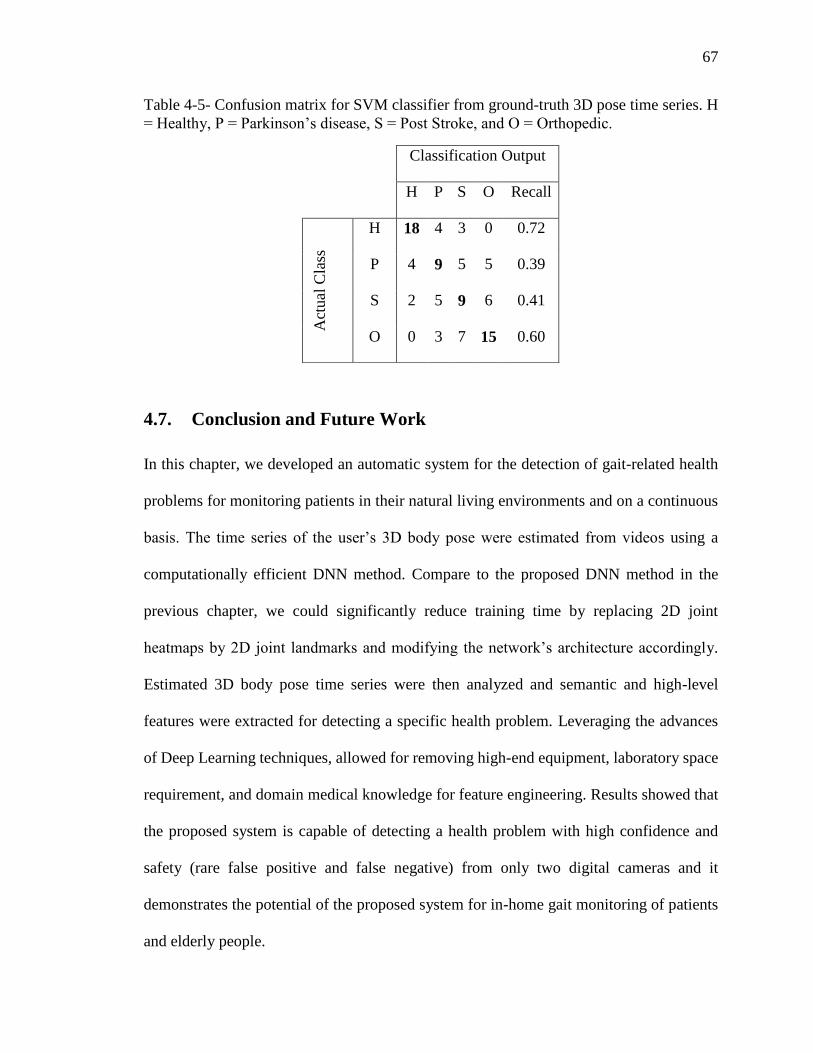
67
Table 4-5- Confusion matrix for SVM classifier from ground-truth 3D pose time series. H
= Healthy, P = Parkinson’s disease, S = Post Stroke, and O = Orthopedic.
Classification Output
H P S O Recall
Act
ual
Cla
ss
H 18 4 3 0 0.72
P 4 9 5 5 0.39
S 2 5 9 6 0.41
O 0 3 7 15 0.60
4.7. Conclusion and Future Work
In this chapter, we developed an automatic system for the detection of gait-related health
problems for monitoring patients in their natural living environments and on a continuous
basis. The time series of the user’s 3D body pose were estimated from videos using a
computationally efficient DNN method. Compare to the proposed DNN method in the
previous chapter, we could significantly reduce training time by replacing 2D joint
heatmaps by 2D joint landmarks and modifying the network’s architecture accordingly.
Estimated 3D body pose time series were then analyzed and semantic and high-level
features were extracted for detecting a specific health problem. Leveraging the advances
of Deep Learning techniques, allowed for removing high-end equipment, laboratory space
requirement, and domain medical knowledge for feature engineering. Results showed that
the proposed system is capable of detecting a health problem with high confidence and
safety (rare false positive and false negative) from only two digital cameras and it
demonstrates the potential of the proposed system for in-home gait monitoring of patients
and elderly people.

68
Despite a large amount of literature devoted to binary gait classification for clinical
application (healthy vs not-healthy) [122, 125, 137], multi-class gait classification is not
well-studied. Compare to the binary gait classification, multi-class gait classification is
more challenging, since it not only needs to recognize the abnormal gait pattern but also
should be able to differentiate between abnormalities. This is not a straightforward task
due to the fact that neurological diseases that interfere with gait pattern display similarities
in gait abnormalities including short steps, leg rigidity, and impaired posture [138]. A few
studies explored the field of machine learning and proposed methods for multi-class gait
classification in order to detect health problems from gait pattern, but these methods
usually need high-end equipment e.g. optical motion capture systems [121] and IMU
sensors [124] to capture body pose time series, which makes them impractical for in-home
use.
Comparing the results of Table 4-3 and Table 4-4 showed that improving the 3D pose
estimation accuracy results in increasing classification performance. Since estimating 3D
body pose from images could be noisy and associate with error, it affects the classification
accuracy. However, the classification performance degradation from estimated 3D body
pose compare to ground-truth 3D body pose was not significant, which demonstrates the
robustness of the proposed classifier to some level of noises.
In contrast to previous studies that use traditional machine learning methods such as
SVM for gait classification [18, 21], our proposed DNN based classifier does not require
feature engineering on the body pose time series. In order to assess the performance of the
proposed classifier, we compared the results with those obtained from SVM as one of the

69
most common machine learning methods for gait classification. Results showed that
classification accuracy improves significantly by applying our DNN-based classifier.
Finally, analyzing of results revealed that Healthy group achieved the best classification
accuracy, while the rest of the groups i.e. Post Stroke, Parkinson, and Orthopedic achieved
comparable accuracies, which are significantly lower than Healthy group. Except for one
false negative and one false positive case, all the misclassifications happened between the
three pathology groups. This happens due to the fact that an altered gait pattern can be
similar between different pathologies and gait alteration due to injuries can be significantly
affected by various events in the gait.
The ultimate goal of this research is to provide an ambient assisted living tool for gait
monitoring of patients and elderly people in the domestic environment by taking
advantages of DNNs. The present study can be considered as a starting point of the research
in this direction and can be used as a basis for future applications of Deep Learning in
clinical gait analysis and pathological gait diagnoses. Future works will focus on expanding
the work by the inclusion of other pathological populations such as Cerebral Palsy.
Cerebral Palsy is a movement disorder that damages parts of the brain that control
movement, balance, and posture. Adults and children with Cerebral Palsy can fall easily
due to balance issues and non-voluntary movements [139, 140]. As a result, they could
benefit from an ambient assisted living system that monitors them constantly to detect
abnormal movement and predict events like falling. Another possible direction for future
work could be improving classification accuracy by adding more input data. Although the
proposed system has high accuracy to distinguish healthy and non-healthy subjects, its
performance for detecting the type of pathology needs improvement. It could be achieved

70
by providing more input data e.g. kinetics information by using wearable force plate
systems or adding the medical history of users to the system by employing Electric Health
Record (HER) data. The latter requires Natural Language Processing (NLP) techniques,
which is an open and fast-growing field of research and has a significant amount of
potential in healthcare applications.

71
CHAPTER 5. Conclusion and Future Work
5.1. Introduction
Human motion capture methods in biomechanics applications have evolved substantially
over recent decades. Limitations of the most widespread motion capture techniques,
namely marker-based motion capture systems, have sparked interest in the development of
marker-less motion capture methods. Considerable developments in computer vision and
in particular Deep Neural Networks have been the motivation of this thesis to propose
marker-less motion capture methods for understanding human motion without the
encumbrance of markers on the subject. In this thesis, by employing DNNs technique, we
proposed two marker-less motion capture methods for human motion analysis in
biomechanics applications. In this chapter, we review and summarize the presented work
and highlight our contributions. We also discuss the future direction of this research.
5.2. Summary of the Thesis
In this thesis, we investigated the applicability of DNNs for two biomechanics
applications including injury prevention (chapter 3) and disease diagnosis (chapter 4).
In chapter 3, we proposed a novel DNN method for 3D human pose estimation from
multi-view images and utilized it for calculating lower back joint loads in order to detect
non-ergonomic movements in the workplaces with the aim of reducing injuries. One of
the key components of our proposed network was hierarchical skip connections. These

72
hierarchical skip connections shared rich information on different scales. Along with the
estimated 2D joint heatmaps, they provided more cues to aid 3D pose estimation. We
applied our proposed method on a Lifting dataset and performed three sets of analysis.
First, analysis of 3D pose generator inputs to assess how the accuracy changes by feeding
more 3D cues to this network. Second, the analysis of 3D pose generator architectures to
find the best network architecture. Third, analysis of lifting type to evaluate the effect of
lifting vertical height and asymmetry angle on the network performance. Then, by applying
inverse dynamics on the estimated 3D pose, we calculated L5/S1 joint moment and force
and compared it with the results of a marker-based motion capture system as a reference.
It was shown that our proposed DNN method provides results comparable with the marker-
based motion capture systems and address their limitations such as being constrained to a
controlled environment or obstructing subject movement by attaching markers.
In chapter 4, we proposed another DNN method for 3D human pose estimation from
multi-view images and utilized it for gait analysis in order to detect walking
abnormalities with the aim of early detection of disease. By replacing estimated 2D joint
heatmaps with 2D joint coordinates, we made the network computationally more efficient
and reduced training time significantly. We applied our proposed method on two different
datasets. First, a gait dataset consists of healthy subjects and patients with three types of
health problems e.g. Parkinson, stroke, and orthopedic. Second, a publicly available dataset
(Human3.6m) in order to compare the performance of our method with other state-of-the-
art methods for 3D human pose estimation. Experimental results revealed that our proposed
method achieved better or comparable performance than other state-of-the-art methods by
employing a novel multi-view fusion technique. We then extended the proposed

73
framework by feeding the estimated 3D body pose into a second network for gait
classification in order to detect gait abnormalities and classify it into the corresponding
health problem. In addition, we performed two sets of analysis. First, analysis of health
problem severity on classification accuracy. Second, analysis of estimated 3D pose on
classification accuracy to assess how the accuracy changes by feeding ground-truth 3D
pose instead of estimated 3D pose to the classifier network. Finally, we compared the
classification results with those obtained from SVM, to evaluate the strength of DNNs for
learning semantic and high-level features from the input data. It was shown that our
proposed framework could classify gait videos with high performance and rare false
positive and false negative rates. It suggests the potential of the proposed framework for
health monitoring of patients and elderly people in their home settings
5.3. Future Work
Future work could aim at proposing a marker-less method for estimating 3D body mesh,
which includes both body pose and body shape from a multi-view or monocular image. 3D
body mesh provides a large number of points on each body segment and enables a more
meaningful motion analysis. In particular, the current method that defines each body
segment with two joints is not capable of motion analyzing in the rotation plane, which is
an important aspect in biomechanics applications.
Another direction for the future work could focus on collecting more data to evaluate the
performance of the proposed method for other types of workplace activities that include
overexertion and repetitive movements and have the potential to lead to injuries (chapter
3), or for evaluating the performance of the proposed method for detecting other types of
neurological diseases such as Cerebral Palsy (chapter 4).

74
5.4. Conclusion Remarks
The present study is a starting point of the research in this direction. The results presented
here demonstrate the potential of DNNs for achieving a level of quantitative accuracy of
human motion analysis that is suitable for biomechanics applications and we believe this
is the viable direction for future study in this field.
The ultimate goal of this thesis is providing a health monitoring system to be utilized in
the workplaces or inside elderly people homes for long-term monitoring of a change in gait
and screening of body posture. This would enable carrying out effective techniques in a
suitable time to prevent injuries and diagnosing movement dysfunctions.

75
References
[1] L. Mündermann, S. Corazza, and T. P. Andriacchi, "The evolution of methods for
the capture of human movement leading to markerless motion capture for
biomechanical applications," Journal of NeuroEngineering and Rehabilitation, vol.
3, p. 6, 2006.
[2] A. Filippeschi, N. Schmitz, M. Miezal, G. Bleser, E. Ruffaldi, and D. Stricker,
"Survey of motion tracking methods based on inertial sensors: a focus on upper
limb human motion," Sensors, vol. 17, p. 1257, 2017.
[3] A. Cappozzo, F. Catani, U. Della Croce, and A. Leardini, "Position and orientation
in space of bones during movement: anatomical frame definition and
determination," Clinical biomechanics, vol. 10, pp. 171-178, 1995.
[4] S. A. Banks and W. A. Hodge, "Accurate measurement of three-dimensional knee
replacement kinematics using single-plane fluoroscopy," IEEE Transactions on
Biomedical Engineering, vol. 43, pp. 638-649, 1996.
[5] S. Bao, N. Howard, P. Spielholz, B. Silverstein, and N. Polissar, "Interrater
reliability of posture observations," Human factors, vol. 51, pp. 292-309, 2009.
[6] Å. Kilbom, "Assessment of physical exposure in relation to work-related
musculoskeletal disorders-what information can be obtained from systematic
observations," Scandinavian journal of work, environment & health, pp. 30-45,
1994.
[7] X. Xu, C.-c. Chang, G. S. Faber, I. Kingma, and J. T. Dennerlein, "The validity and
interrater reliability of video-based posture observation during asymmetric lifting
tasks," Human Factors, vol. 53, pp. 371-382, 2011.
[8] F. Ferrarello, V. A. M. Bianchi, M. Baccini, G. Rubbieri, E. Mossello, M. C.
Cavallini, et al., "Tools for observational gait analysis in patients with stroke: a
systematic review," Physical therapy, vol. 93, pp. 1673-1685, 2013.
[9] S. M. Hsiang, G. E. Brogmus, S. E. Martin, and I. B. Bezverkhny, "Video based
lifting technique coding system," Ergonomics, vol. 41, pp. 239-256, 1998.
[10] P. Coenen, I. Kingma, C. R. Boot, P. M. Bongers, and J. H. van Dieën, "Inter-rater
reliability of a video-analysis method measuring low-back load in a field situation,"
Applied ergonomics, vol. 44, pp. 828-834, 2013.
[11] C.-C. Chang, S. Hsiang, P. G. Dempsey, and R. W. McGorry, "A computerized
video coding system for biomechanical analysis of lifting tasks," International
Journal of Industrial Ergonomics, vol. 32, pp. 239-250, 2003.
[12] T. B. Moeslund, A. Hilton, and V. Krüger, "A survey of advances in vision-based
human motion capture and analysis," Computer vision and image understanding,
vol. 104, pp. 90-126, 2006.
[13] R. Poppe, "Vision-based human motion analysis: An overview," Computer vision
and image understanding, vol. 108, pp. 4-18, 2007.
[14] N. Sarafianos, B. Boteanu, B. Ionescu, and I. A. Kakadiaris, "3d human pose
estimation: A review of the literature and analysis of covariates," Computer Vision
and Image Understanding, vol. 152, pp. 1-20, 2016.

76
[15] M. Baccouche, F. Mamalet, C. Wolf, C. Garcia, and A. Baskurt, "Sequential deep
learning for human action recognition," in International Workshop on Human
Behavior Understanding, 2011, pp. 29-39.
[16] J. Yang, M. N. Nguyen, P. P. San, X. Li, and S. Krishnaswamy, "Deep
Convolutional Neural Networks on Multichannel Time Series for Human Activity
Recognition," in IJCAI, 2015, pp. 3995-4001.
[17] Y. Xu, T. Mo, Q. Feng, P. Zhong, M. Lai, I. Eric, et al., "Deep learning of feature
representation with multiple instance learning for medical image analysis," in
Acoustics, Speech and Signal Processing (ICASSP), 2014 IEEE International
Conference on, 2014, pp. 1626-1630.
[18] X. Peng, Z. Tang, F. Yang, R. S. Feris, and D. Metaxas, "Jointly optimize data
augmentation and network training: Adversarial data augmentation in human pose
estimation," in Proceedings of the IEEE Conference on Computer Vision and
Pattern Recognition, 2018, pp. 2226-2234.
[19] Z. Tang, X. Peng, S. Geng, L. Wu, S. Zhang, and D. Metaxas, "Quantized densely
connected u-nets for efficient landmark localization," in Proceedings of the
European Conference on Computer Vision (ECCV), 2018, pp. 339-354.
[20] E. Brau and H. Jiang, "3d human pose estimation via deep learning from 2d
annotations," in 2016 Fourth International Conference on 3D Vision (3DV), 2016,
pp. 582-591.
[21] B. Tekin, P. Marquez Neila, M. Salzmann, and P. Fua, "Learning to fuse 2d and 3d
image cues for monocular body pose estimation," in International Conference on
Computer Vision (ICCV), 2017.
[22] J. O'rourke and N. I. Badler, "Model-based image analysis of human motion using
constraint propagation," IEEE Transactions on Pattern Analysis and Machine
Intelligence, pp. 522-536, 1980.
[23] K. Rohr, "Towards model-based recognition of human movements in image
sequences," CVGIP: Image understanding, vol. 59, pp. 94-115, 1994.
[24] L. Sigal, A. O. Balan, and M. J. Black, "Humaneva: Synchronized video and motion
capture dataset and baseline algorithm for evaluation of articulated human motion,"
International journal of computer vision, vol. 87, p. 4, 2010.
[25] J. Deutscher and I. Reid, "Articulated body motion capture by stochastic search,"
International Journal of Computer Vision, vol. 61, pp. 185-205, 2005.
[26] V. John and E. Trucco, "Multiple view human articulated tracking using charting
and particle swarm optimisation," in Proceedings of the 1st international workshop
on 3D video processing, 2010, pp. 51-56.
[27] L. Sigal, M. Isard, H. Haussecker, and M. J. Black, "Loose-limbed people:
Estimating 3d human pose and motion using non-parametric belief propagation,"
International journal of computer vision, vol. 98, pp. 15-48, 2012.
[28] A. Moutzouris, J. Martinez-del-Rincon, J.-C. Nebel, and D. Makris, "Efficient
tracking of human poses using a manifold hierarchy," Computer Vision and Image
Understanding, vol. 132, pp. 75-86, 2015.
[29] W. Zhang, L. Shang, and A. B. Chan, "A robust likelihood function for 3D human
pose tracking," IEEE Transactions on Image Processing, vol. 23, pp. 5374-5389,
2014.

77
[30] J. Gall, B. Rosenhahn, T. Brox, and H.-P. Seidel, "Optimization and filtering for
human motion capture," International journal of computer vision, vol. 87, p. 75,
2010.
[31] J. Müller and M. Arens, "Human pose estimation with implicit shape models," in
Proceedings of the first ACM international workshop on Analysis and retrieval of
tracked events and motion in imagery streams, 2010, pp. 9-14.
[32] S. Amin, M. Andriluka, M. Rohrbach, and B. Schiele, "Multi-view Pictorial
Structures for 3D Human Pose Estimation," in Bmvc, 2013.
[33] J. Deutscher, A. Blake, and I. Reid, "Articulated body motion capture by annealed
particle filtering," in Computer Vision and Pattern Recognition, 2000. Proceedings.
IEEE Conference on, 2000, pp. 126-133.
[34] A. Elgammal and C.-S. Lee, "Tracking people on a torus," IEEE Transactions on
Pattern Analysis and Machine Intelligence, vol. 31, pp. 520-538, 2009.
[35] C. Gonzales and S. Dubuisson, "Combinatorial resampling particle filter: An
effective and efficient method for articulated object tracking," International
Journal of Computer Vision, vol. 112, pp. 255-284, 2015.
[36] L. Raskin, M. Rudzsky, and E. Rivlin, "Dimensionality reduction using a Gaussian
Process Annealed Particle Filter for tracking and classification of articulated body
motions," Computer Vision and Image Understanding, vol. 115, pp. 503-519, 2011.
[37] A. Bangian-Tabrizi and Y. Jaluria, "An optimization strategy for the inverse
solution of a convection heat transfer problem," International Journal of Heat and
Mass Transfer, vol. 124, pp. 1147-1155, 2018.
[38] A. Bangian-Tabrizi and Y. Jaluria, "A study of transient wall plume and its
application in the solution of inverse problems," Numerical Heat Transfer, Part A:
Applications, vol. 75, pp. 149-166, 2019.
[39] Y. Jaluria and A. Tabrizi, "Transient Flow in a Wall Plume and its Application to
Solve an Inverse Problem," Bulletin of the American Physical Society, 2018.
[40] B. Kwolek, T. Krzeszowski, A. Gagalowicz, K. Wojciechowski, and H. Josinski,
"Real-time multi-view human motion tracking using particle swarm optimization
with resampling," in International Conference on Articulated Motion and
Deformable Objects, 2012, pp. 92-101.
[41] B. Rymut and B. Kwolek, "Real‐time multiview human pose tracking using
graphics processing unit‐accelerated particle swarm optimization," Concurrency
and Computation: Practice and Experience, vol. 27, pp. 1551-1563, 2015.
[42] S. Saini, N. Zakaria, D. R. A. Rambli, and S. Sulaiman, "Markerless human motion
tracking using hierarchical multi-swarm cooperative particle swarm optimization,"
PloS one, vol. 10, p. e0127833, 2015.
[43] T. Krzeszowski, B. Kwolek, and K. Wojciechowski, "Articulated body motion
tracking by combined particle swarm optimization and particle filtering," in
International Conference on Computer Vision and Graphics, 2010, pp. 147-154.
[44] X. Wang, W. Wan, X. Zhang, and X. Yu, "Annealed particle filter based on particle
swarm optimization for articulated three-dimensional human motion tracking,"
Optical Engineering, vol. 49, pp. 017204-017204-11, 2010.
[45] J. MacCormick and M. Isard, "Partitioned sampling, articulated objects, and
interface-quality hand tracking," in European Conference on Computer Vision,
2000, pp. 3-19.

78
[46] Y. Li and Z. Sun, "Articulated Human Motion Tracking Using Sequential Immune
Genetic Algorithm," Mathematical Problems in Engineering, vol. 2013, 2013.
[47] X. Zhao and Y. Liu, "Generative tracking of 3D human motion by hierarchical
annealed genetic algorithm," Pattern Recognition, vol. 41, pp. 2470-2483, 2008.
[48] S. Sedai, "Human motion capture in images and videos using discriminative and
hybrid learning methods," 2012.
[49] P. Kohli, J. Rihan, M. Bray, and P. H. Torr, "Simultaneous segmentation and pose
estimation of humans using dynamic graph cuts," International Journal of
Computer Vision, vol. 79, pp. 285-298, 2008.
[50] R. Urtasun, D. J. Fleet, A. Hertzmann, and P. Fua, "Priors for people tracking from
small training sets," in Computer Vision, 2005. ICCV 2005. Tenth IEEE
International Conference on, 2005, pp. 403-410.
[51] R. Mehrizi, X. Peng, X. Xu, S. Zhang, D. Metaxas, and K. Li, "A computer vision
based method for 3D posture estimation of symmetrical lifting," Journal of
Biomechanics, vol. 69, pp. 40-46, 2018.
[52] K. Grauman, G. Shakhnarovich, and T. Darrell, "Inferring 3d structure with a
statistical image-based shape model," in null, 2003, p. 641.
[53] J.-B. Huang and M.-H. Yang, "Estimating human pose from occluded images," in
Asian Conference on Computer Vision, 2009, pp. 48-60.
[54] A. Agarwal and B. Triggs, "Recovering 3D human pose from monocular images,"
IEEE transactions on pattern analysis and machine intelligence, vol. 28, pp. 44-
58, 2006.
[55] R. Rosales and S. Sclaroff, "Learning body pose via specialized maps," in Advances
in neural information processing systems, 2001, pp. 1263-1270.
[56] N. Dalal and B. Triggs, "Histograms of oriented gradients for human detection," in
Computer Vision and Pattern Recognition, 2005. CVPR 2005. IEEE Computer
Society Conference on, 2005, pp. 886-893.
[57] L. Bo and C. Sminchisescu, "Twin gaussian processes for structured prediction,"
International Journal of Computer Vision, vol. 87, pp. 28-52, 2010.
[58] A. Kanaujia, C. Sminchisescu, and D. Metaxas, "Semi-supervised hierarchical
models for 3d human pose reconstruction," in 2007 IEEE Conference on Computer
Vision and Pattern Recognition, 2007, pp. 1-8.
[59] A. Elgammal and C.-S. Lee, "Inferring 3D body pose from silhouettes using activity
manifold learning," in Computer Vision and Pattern Recognition, 2004. CVPR
2004. Proceedings of the 2004 IEEE Computer Society Conference on, 2004, pp.
II-681-II-688 Vol. 2.
[60] J. B. Tenenbaum, V. De Silva, and J. C. Langford, "A global geometric framework
for nonlinear dimensionality reduction," science, vol. 290, pp. 2319-2323, 2000.
[61] R. Li, T.-P. Tian, S. Sclaroff, and M.-H. Yang, "3d human motion tracking with a
coordinated mixture of factor analyzers," International Journal of Computer
Vision, vol. 87, pp. 170-190, 2010.
[62] X. Peng, S. Zhang, Y. Yang, and D. N. Metaxas, "Piefa: Personalized incremental
and ensemble face alignment," in Proceedings of the IEEE International
Conference on Computer Vision, 2015, pp. 3880-3888.

79
[63] X. Peng, R. S. Feris, X. Wang, and D. N. Metaxas, "A recurrent encoder-decoder
network for sequential face alignment," in European conference on computer
vision, 2016, pp. 38-56.
[64] X. Peng, J. Huang, Q. Hu, S. Zhang, and D. N. Metaxas, "Three-dimensional head
pose estimation in-the-wild," in Automatic Face and Gesture Recognition (FG),
2015 11th IEEE International Conference and Workshops on, 2015, pp. 1-6.
[65] X. Peng, J. Huang, Q. Hu, S. Zhang, A. Elgammal, and D. Metaxas, "From circle
to 3-sphere: Head pose estimation by instance parameterization," Computer Vision
and Image Understanding, vol. 136, pp. 92-102, 2015.
[66] W.-K. Liao and G. Medioni, "3D face tracking and expression inference from a 2D
sequence using manifold learning," in Computer Vision and Pattern Recognition,
2008. CVPR 2008. IEEE Conference on, 2008, pp. 1-8.
[67] H. Ning, W. Xu, Y. Gong, and T. Huang, "Discriminative learning of visual words
for 3D human pose estimation," in Computer Vision and Pattern Recognition, 2008.
CVPR 2008. IEEE Conference on, 2008, pp. 1-8.
[68] G. Antipov, S.-A. Berrani, N. Ruchaud, and J.-L. Dugelay, "Learned vs. hand-
crafted features for pedestrian gender recognition," in Proceedings of the 23rd ACM
international conference on Multimedia, 2015, pp. 1263-1266.
[69] A. B. Sargano, P. Angelov, and Z. Habib, "A comprehensive review on handcrafted
and learning-based action representation approaches for human activity
recognition," Applied Sciences, vol. 7, p. 110, 2017.
[70] S. Li and A. B. Chan, "3d human pose estimation from monocular images with deep
convolutional neural network," in Asian Conference on Computer Vision, 2014, pp.
332-347.
[71] B. Tekin, A. Rozantsev, V. Lepetit, and P. Fua, "Direct prediction of 3d body poses
from motion compensated sequences," in Proceedings of the IEEE Conference on
Computer Vision and Pattern Recognition, 2016, pp. 991-1000.
[72] A. Krizhevsky, I. Sutskever, and G. E. Hinton, "Imagenet classification with deep
convolutional neural networks," in Advances in neural information processing
systems, 2012, pp. 1097-1105.
[73] G. Rogez and C. Schmid, "MoCap-guided data augmentation for 3D pose
estimation in the wild," in Advances in Neural Information Processing Systems,
2016, pp. 3108-3116.
[74] A. Bulat and G. Tzimiropoulos, "Human pose estimation via convolutional part
heatmap regression," in European Conference on Computer Vision, 2016, pp. 717-
732.
[75] A. Newell, K. Yang, and J. Deng, "Stacked hourglass networks for human pose
estimation," in European Conference on Computer Vision, 2016, pp. 483-499.
[76] S.-E. Wei, V. Ramakrishna, T. Kanade, and Y. Sheikh, "Convolutional pose
machines," in Proceedings of the IEEE Conference on Computer Vision and
Pattern Recognition, 2016, pp. 4724-4732.
[77] C.-H. Chen and D. Ramanan, "3d human pose estimation= 2d pose estimation+
matching," in CVPR, 2017, p. 6.
[78] S. Park, J. Hwang, and N. Kwak, "3D human pose estimation using convolutional
neural networks with 2D pose information," in European Conference on Computer
Vision, 2016, pp. 156-169.

80
[79] C. Wang, Y. Wang, Z. Lin, A. L. Yuille, and W. Gao, "Robust estimation of 3d
human poses from a single image," in Proceedings of the IEEE Conference on
Computer Vision and Pattern Recognition, 2014, pp. 2361-2368.
[80] J. Martinez, R. Hossain, J. Romero, and J. J. Little, "A simple yet effective baseline
for 3d human pose estimation," in International Conference on Computer Vision,
2017, p. 5.
[81] G. Pavlakos, X. Zhou, K. G. Derpanis, and K. Daniilidis, "Coarse-to-fine
volumetric prediction for single-image 3D human pose," in Computer Vision and
Pattern Recognition (CVPR), 2017 IEEE Conference on, 2017, pp. 1263-1272.
[82] D. Tome, C. Russell, and L. Agapito, "Lifting from the deep: Convolutional 3d
pose estimation from a single image," CVPR 2017 Proceedings, pp. 2500-2509,
2017.
[83] V. Belagiannis and A. Zisserman, "Recurrent human pose estimation," in
Automatic Face & Gesture Recognition (FG 2017), 2017 12th IEEE International
Conference on, 2017, pp. 468-475.
[84] G. Pavlakos, X. Zhou, K. G. Derpanis, and K. Daniilidis, "Coarse-to-fine
volumetric prediction for single-image 3D human pose," arXiv preprint
arXiv:1611.07828, 2016.
[85] G. Papandreou, T. Zhu, N. Kanazawa, A. Toshev, J. Tompson, C. Bregler, et al.,
"Towards accurate multi-person pose estimation in the wild," in Proceedings of the
IEEE Conference on Computer Vision and Pattern Recognition, 2017, pp. 4903-
4911.
[86] X. Zhou, Q. Huang, X. Sun, X. Xue, and Y. Wei, "Towards 3d human pose
estimation in the wild: a weakly-supervised approach," in Proceedings of the IEEE
International Conference on Computer Vision, 2017, pp. 398-407.
[87] S. Corazza, L. Muendermann, A. Chaudhari, T. Demattio, C. Cobelli, and T. P.
Andriacchi, "A markerless motion capture system to study musculoskeletal
biomechanics: visual hull and simulated annealing approach," Annals of biomedical
engineering, vol. 34, pp. 1019-1029, 2006.
[88] M. Sandau, H. Koblauch, T. B. Moeslund, H. Aanæs, T. Alkjær, and E. B.
Simonsen, "Markerless motion capture can provide reliable 3D gait kinematics in
the sagittal and frontal plane," Medical Engineering and Physics, vol. 36, pp. 1168-
1175, 2014.
[89] E. Ceseracciu, Z. Sawacha, S. Fantozzi, M. Cortesi, G. Gatta, S. Corazza, et al.,
"Markerless analysis of front crawl swimming," Journal of biomechanics, vol. 44,
pp. 2236-2242, 2011.
[90] A. Drory, H. Li, and R. Hartley, "A learning-based markerless approach for full-
body kinematics estimation in-natura from a single image," Journal of
biomechanics, vol. 55, pp. 1-10, 2017.
[91] R. Mehrizi, X. Peng, Z. Tang, X. Xu, D. Metaxas, and K. Li, "Toward Marker-free
3D Pose Estimation in Lifting: A Deep Multi-view Solution," in Automatic Face &
Gesture Recognition (FG 2018), 2018 13th IEEE International Conference on,
2018, pp. 485-491.
[92] X. Xu, C.-C. Chang, G. S. Faber, I. Kingma, and J. T. Dennerlein, "Estimating 3-
D L5/S1 Moments During Manual Lifting Using a Video Coding System: Validity
and Interrater Reliability," Human factors, vol. 54, pp. 1053-1065, 2012.

81
[93] A. Toshev and C. Szegedy, "Deeppose: Human pose estimation via deep neural
networks," in Proceedings of the IEEE conference on computer vision and pattern
recognition, 2014, pp. 1653-1660.
[94] J. J. Tompson, A. Jain, Y. LeCun, and C. Bregler, "Joint training of a convolutional
network and a graphical model for human pose estimation," in Advances in neural
information processing systems, 2014, pp. 1799-1807.
[95] J. Carreira, P. Agrawal, K. Fragkiadaki, and J. Malik, "Human pose estimation with
iterative error feedback," in Proceedings of the IEEE conference on computer
vision and pattern recognition, 2016, pp. 4733-4742.
[96] H. Noh, S. Hong, and B. Han, "Learning deconvolution network for semantic
segmentation," in Proceedings of the IEEE International Conference on Computer
Vision, 2015, pp. 1520-1528.
[97] J. Yang, S. E. Reed, M.-H. Yang, and H. Lee, "Weakly-supervised disentangling
with recurrent transformations for 3d view synthesis," in Advances in Neural
Information Processing Systems, 2015, pp. 1099-1107.
[98] K. He, X. Zhang, S. Ren, and J. Sun, "Deep residual learning for image
recognition," in Proceedings of the IEEE conference on computer vision and
pattern recognition, 2016, pp. 770-778.
[99] D. Tome, C. Russell, and L. Agapito, "Lifting from the deep: Convolutional 3d
pose estimation from a single image," arXiv preprint arXiv:1701.00295, 2017.
[100] X. Zhou, Q. Huang, X. Sun, X. Xue, and Y. Wei, "Towards 3D Human Pose
Estimation in the Wild: a Weakly-supervised Approach," in International
Conference on Computer Vision, 2017.
[101] Z. Zhang, "A flexible new technique for camera calibration," IEEE Transactions
on pattern analysis and machine intelligence, vol. 22, 2000.
[102] D. P. Kingma and J. Ba, "Adam: A method for stochastic optimization," arXiv
preprint arXiv:1412.6980, 2014.
[103] M. Andriluka, L. Pishchulin, P. Gehler, and B. Schiele, "2d human pose estimation:
New benchmark and state of the art analysis," in Proceedings of the IEEE
Conference on computer Vision and Pattern Recognition, 2014, pp. 3686-3693.
[104] R. Mehrizi, X. Peng, X. Xu, S. Zhang, and K. Li, "A Deep Neural Network-based
method for estimation of 3D lifting motions," Journal of biomechanics, vol. 84, pp.
87-93, 2019.
[105] L. Manchikanti, V. Singh, F. J. Falco, R. M. Benyamin, and J. A. Hirsch,
"Epidemiology of low back pain in adults," Neuromodulation: Technology at the
Neural Interface, vol. 17, pp. 3-10, 2014.
[106] J. I. Kuiper, A. Burdorf, J. H. Verbeek, M. H. Frings-Dresen, A. J. van der Beek,
and E. R. Viikari-Juntura, "Epidemiologic evidence on manual materials handling
as a risk factor for back disorders: a systematic review," International Journal of
Industrial Ergonomics, vol. 24, pp. 389-404, 1999.
[107] B. R. Da Costa, and Edgar Ramos Vieira, "Risk factors for work‐related
musculoskeletal disorders: a systematic review of recent longitudinal studies,"
American journal of industrial medicine vol. 53.3, pp. 285-323, 2010.
[108] W. Marras, L. Fine, S. Ferguson, and T. Waters, "The effectiveness of commonly
used lifting assessment methods to identify industrial jobs associated with elevated
risk of low-back disorders," Ergonomics, vol. 42, pp. 229-245, 1999.

82
[109] P. De Leva, "Adjustments to Zatsiorsky-Seluyanov's segment inertia parameters,"
Journal of biomechanics, vol. 29.9, pp. 1223-1230, 1996.
[110] A. L. Hof, "An explicit expression for the moment in multibody systems," Journal
of biomechanics, vol. 25.10, pp. 1209-1211, 1992.
[111] R. Mehrizi, X. Xu, S. Zhang, V. Pavlovic, D. Metaxas, and K. Li, "Using a marker-
less method for estimating L5/S1 moments during symmetrical lifting," Applied
ergonomics, 2017.
[112] M. De Looze, I. Kingma, J. Bussmann, and H. Toussaint, "Validation of a dynamic
linked segment model to calculate joint moments in lifting," Clinical Biomechanics,
vol. 7, pp. 161-169, 1992.
[113] M. Häkkänen, E. Viikari-Juntura, and E.-P. Takala, "Effects of changes in work
methods on musculoskeletal load. An intervention study in the trailer assembly,"
Applied Ergonomics, vol. 28, pp. 99-108, 1997.
[114] S. A. Lavender, G. B. Andersson, O. D. Schipplein, and H. J. Fuentes, "The effects
of initial lifting height, load magnitude, and lifting speed on the peak dynamic
L5/S1 moments," International Journal of Industrial Ergonomics, vol. 31, pp. 51-
59, 2003.
[115] G. Shin and G. Mirka, "The effects of a sloped ground surface on trunk kinematics
and L5/S1 moment during lifting," Ergonomics, vol. 47, pp. 646-659, 2004.
[116] J. L. Fleiss, Design and analysis of clinical experiments, vol. Vol. 73. John Wiley
& Sons, 2011.
[117] B. D. Hendershot, and Erik J. Wolf, "Three-dimensional joint reaction forces and
moments at the low back during over-ground walking in persons with unilateral
lower-extremity amputation," Clinical Biomechanics vol. 29.3, pp. 235-242, 2014.
[118] I. Shojaei, Vazirian, M., Croft, E., Nussbaum, M. A., & Bazrgari, B., "Age related
differences in mechanical demands imposed on the lower back by manual material
handling tasks," Journal of biomechanics, vol. 49, pp. 896-903, 2016.
[119] R. Mehrizi, X. Peng, D. N. Metaxas, X. Xu, S. Zhang, and K. Li, "Predicting 3-D
Lower Back Joint Load in Lifting: A Deep Pose Estimation Approach," IEEE
Transactions on Human-Machine Systems, vol. 49, pp. 85-94, 2019.
[120] A. Muro-De-La-Herran, B. Garcia-Zapirain, and A. Mendez-Zorrilla, "Gait
analysis methods: An overview of wearable and non-wearable systems,
highlighting clinical applications," Sensors, vol. 14, pp. 3362-3394, 2014.
[121] B. Pogorelc, Z. Bosnić, and M. Gams, "Automatic recognition of gait-related health
problems in the elderly using machine learning," Multimedia Tools and
Applications, vol. 58, pp. 333-354, 2012.
[122] R. LeMoyne, W. Kerr, T. Mastroianni, and A. Hessel, "Implementation of machine
learning for classifying hemiplegic gait disparity through use of a force plate," in
Machine Learning and Applications (ICMLA), 2014 13th International Conference
on, 2014, pp. 379-382.
[123] S. Shetty and Y. Rao, "SVM based machine learning approach to identify
Parkinson's disease using gait analysis," in Inventive Computation Technologies
(ICICT), International Conference on, 2016, pp. 1-5.
[124] A. Mannini, D. Trojaniello, A. Cereatti, and A. M. Sabatini, "A machine learning
framework for gait classification using inertial sensors: Application to elderly, post-
stroke and huntington’s disease patients," Sensors, vol. 16, p. 134, 2016.

83
[125] H. H. Manap, N. M. Tahir, A. I. M. Yassin, and R. Abdullah, "Anomaly gait
classification of parkinson disease based on ann," in System Engineering and
Technology (ICSET), 2011 IEEE International Conference on, 2011, pp. 5-9.
[126] M. Daneshzand, "Delayed Feedback Frequency Adjustment for Deep Brain
Stimulation of Subthalamic Nucleus Oscillations," in 2018 40th Annual
International Conference of the IEEE Engineering in Medicine and Biology Society
(EMBC), 2018, pp. 2194-2197.
[127] M. Daneshzand, M. Faezipour, and B. D. Barkana, "Robust desynchronization of
Parkinson’s disease pathological oscillations by frequency modulation of delayed
feedback deep brain stimulation," PloS one, vol. 13, p. e0207761, 2018.
[128] M. Daneshzand, M. Faezipour, and B. D. Barkana, "Towards frequency adaptation
for delayed feedback deep brain stimulations," Neural regeneration research, vol.
13, p. 408, 2018.
[129] C. Ionescu, D. Papava, V. Olaru, and C. Sminchisescu, "Human3. 6m: Large scale
datasets and predictive methods for 3d human sensing in natural environments,"
IEEE transactions on pattern analysis and machine intelligence, vol. 36, pp. 1325-
1339, 2014.
[130] V. Nair and G. E. Hinton, "Rectified linear units improve restricted boltzmann
machines," in Proceedings of the 27th international conference on machine
learning (ICML-10), 2010, pp. 807-814.
[131] S. Ioffe and C. Szegedy, "Batch normalization: Accelerating deep network training
by reducing internal covariate shift," arXiv preprint arXiv:1502.03167, 2015.
[132] N. Srivastava, G. Hinton, A. Krizhevsky, I. Sutskever, and R. Salakhutdinov,
"Dropout: a simple way to prevent neural networks from overfitting," The Journal
of Machine Learning Research, vol. 15, pp. 1929-1958, 2014.
[133] Z. Wang, W. Yan, and T. Oates, "Time series classification from scratch with deep
neural networks: A strong baseline," in 2017 International Joint Conference on
Neural Networks (IJCNN), 2017, pp. 1578-1585.
[134] K. He, X. Zhang, S. Ren, and J. Sun, "Delving deep into rectifiers: Surpassing
human-level performance on imagenet classification," in Proceedings of the IEEE
international conference on computer vision, 2015, pp. 1026-1034.
[135] G. Pavlakos, X. Zhou, K. G. Derpanis, and K. Daniilidis, "Harvesting multiple
views for marker-less 3d human pose annotations," arXiv preprint
arXiv:1704.04793, 2017.
[136] X. Zhou, M. Zhu, S. Leonardos, K. G. Derpanis, and K. Daniilidis, "Sparseness
meets deepness: 3D human pose estimation from monocular video," in Proceedings
of the IEEE conference on computer vision and pattern recognition, 2016, pp.
4966-4975.
[137] J. Ajay, C. Song, A. Wang, J. Langan, Z. Li, and W. Xu, "A pervasive and sensor-
free Deep Learning system for Parkinsonian gait analysis," in Biomedical & Health
Informatics (BHI), 2018 IEEE EMBS International Conference on, 2018, pp. 108-
111.
[138] H. Stolze, J. P. Kuhtz-Buschbeck, H. Drücke, K. Jöhnk, M. Illert, and G. Deuschl,
"Comparative analysis of the gait disorder of normal pressure hydrocephalus and
Parkinson's disease," Journal of Neurology, Neurosurgery & Psychiatry, vol. 70,
pp. 289-297, 2001.

84
[139] Y. Chiba, A. Shimada, F. Yoshida, H. Keino, M. Hasegawa, H. Ikari, et al., "Risk
of fall for individuals with intellectual disability," American Journal on Intellectual
and Developmental Disabilities, vol. 114, pp. 225-236, 2009.
[140] M. Bottos, A. Feliciangeli, L. Sciuto, C. Gericke, and A. Vianello, "Functional
status of adults with cerebral palsy and implications for treatment of children,"
Developmental medicine and child neurology, vol. 43, pp. 516-528, 2001.