decorrelating wireless sensor network trafﬁc to inhibit …rhan/papers/deng_traffic_pmc.pdf ·...

Elsevier Pervasive and Mobile Computing Journal, Special Issue on Security in Wireless Mobile ComputingSystems, vol 2, issue 2, April 2006, pp. 159-186

Decorrelating Wireless Sensor Network Traffic To InhibitTraffic Analysis Attacks

Jing Deng Richard Han Shivakant MishraDepartment of Computer ScienceUniversity of Colorado at Boulder

Boulder, Colorado, USA{jing,rhan,mishras}@cs.colorado.edu

Abstract

Typical packet traffic in a sensor network reveals pronouncedpatterns that allow an adversary analyzingpacket traffic to deduce the location of a base station. Once discovered, the base station can be destroyed,rendering the entire sensor network inoperative, since a base station is a central point of data collectionand hence failure. This paper investigates a suite of decorrelation countermeasures aimed at disguisingthe location of a base station against traffic analysis attacks. A set of basic countermeasures is described,including hop-by-hop reencryption of the packet to change its appearance, imposition of a uniform packetsending rate, and removal of correlation between a packet’sreceipt time and its forwarding time. Moresophisticated countermeasures are described that introduce randomness into the path taken by a packet.Packets may also fork into multiple fake paths to further confuse an adversary. A technique is introducedto create multiple random areas of high communication activity called hot spots to deceive an adversary asto the true location of the base station. The effectiveness of these countermeasures against traffic analysisattacks is demonstrated analytically and via simulation using three evaluation criteria: total entropy of thenetwork, total overhead/energy consumed, and the ability to frustrate heuristic-based search techniques tolocate a base station.

Keywords: Sensor Network Security, Traffic Analysis

1 Introduction

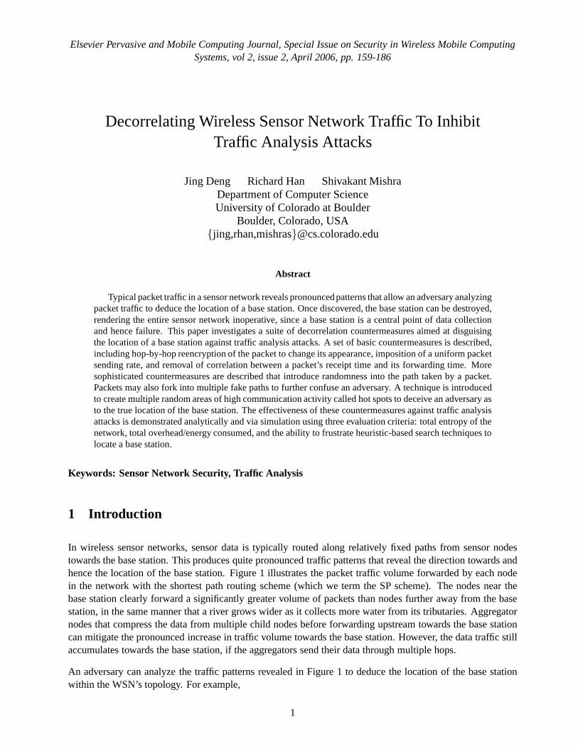
In wireless sensor networks, sensor data is typically routed along relatively fixed paths from sensor nodestowards the base station. This produces quite pronounced traffic patterns that reveal the direction towards andhence the location of the base station. Figure 1 illustratesthe packet traffic volume forwarded by each nodein the network with the shortest path routing scheme (which we term the SP scheme). The nodes near thebase station clearly forward a significantly greater volumeof packets than nodes further away from the basestation, in the same manner that a river grows wider as it collects more water from its tributaries. Aggregatornodes that compress the data from multiple child nodes before forwarding upstream towards the base stationcan mitigate the pronounced increase in traffic volume towards the base station. However, the data traffic stillaccumulates towards the base station, if the aggregators send their data through multiple hops.

An adversary can analyze the traffic patterns revealed in Figure 1 to deduce the location of the base stationwithin the WSN’s topology. For example,

1


0

20

40

60

80

0

20

40

60

800

50

100

150

200

250

300

350

base station area A path to base station

A node which issending data

A node which doesn’t send data 10 20 30 40 50 60 70 80

10

20

30

40

50

60

70

80

40

80

120

(a) 3-D graph of data traffic. (b) Contour map of data traffic.

Figure 1: Pronounced data traffic patterns in a WSN using SP routing scheme reveal the location of the basestation.

1. If the contents of a packet being transmitted are in plain text, an adversary can determine which packetsare being forwarded towards the base station. This allows the adversary to follow the direction of thesepackets towards the base station.

2. If there is a correlation in time between the instant a nodeX receives a packet (a neighbor transmitsthat packet toX) and when nodeX forwards that packet, an adversary can use this time correlation toidentify the same packet as it is relayed hop by hop, and thereby trace the direction towards the basestation.

3. Given that there is higher communication activity near the base station, an adversary can move closerto the base station by moving towards areas of higher packet traffic.

Since the base station is a central point of failure, once thelocation of the base station is discovered, anadversary can disable or destroy the base station, thereby rendering ineffective the data-gathering duties ofthe entire sensor network.

A simple defense against plaintext observation is to encrypt each packet. However, if data packets are en-crypted, but do not change hop by hop, then an adversary can still follow a given encrypted packet patterntowards its destination, which will often wind up at the basestation. Following the path of encrypted packetscan be defeated if each data packet is reencrypted at each hop, thereby changing the appearance of each packetat each hop, e.g. by employing pair-wise key schemes [8, 3, 7,14, 25].

Even with hop-by-hop reencrypted packets, an adversary canstill deduce significant information that canreveal the base station’s location by monitoring traffic volume, or by looking at time correlations. The act oftransmitting itself reveals information to the attacker, regardless of whether packet contents can be inspected.In the case of rate monitoring, the volume of transmissions can be exploited. In the case of time correlation,an adversary can listen to a transmission and also the next-hop forwarding transmission along a relay path andinfer some path relationship between two neighboring nodesregardless of whether the packet is redisguisedat each hop.

We therefore identify two classes of traffic analysis attacks in wireless sensor networks, arate monitoring

2


attack and atime correlationattack. In arate monitoringattack, an adversary monitors the packet sendingrate of nodes near the adversary, and moves closer to the nodes that have a higher packet sending rate. In atimecorrelationattack, an adversary observes the correlation in sending time between a node and its neighboringnode that is assumed to be forwarding the same packet, and infers the path by following the “sound” of eachforwarding operation as the packet propagates towards the base station.

In this paper, we focus on developing countermeasures against traffic analysis attacks that seek to locate thebase station, particularly against the rate monitoring andtime correlation attacks. Given an adversary whois analyzing packet transmissions within its range, the overall objective is to significantly delay an adversaryfrom locating a base station. In particular, our goals are:

• An adversary cannot determine a packet destination by inspecting the contents of the packet.

• An adversary cannot find the data flow direction by analyzing the time correlation between the packetssent by children nodes and packets sent by their parent nodes.

• An adversary cannot find the data transmission direction by employing statistical analysis of the packettransmission rate of every node within its range.

One way to defend against traffic analysis is to control the packet sending rate of every node in the networkin such a way that every node sends packets with the same rate.In Section 3, we describe two methods tocontrol the packet sending rate and packet sending time of each sensor node. These two methods can be usedto defend against the rate monitoring and time correlation attacks. However, there are some limitations tothese rate control methods. For example, they may delay datareports, or introduce too much traffic to thenetwork.

To address these limitations, we propose four improved techniques in Section 4 that introduce randomizedtraffic volumes throughout the sensor network to deceive or misdirect an adversary from discovering the truelocation of the base station. First, a multiple parent routing scheme is introduced that allows a sensor node toforward a packet to one of its parents. This makes the patterns less pronounced in terms of routing packetstowards the base station. Second, a controlled random walk is introduced into the multi-hop path traversedby a packet through the WSN towards the base station. This distributes packet traffic, thereby renderingless effective rate monitoring attacks. Third, random fakepaths are introduced to confuse an adversary fromtracking a packet as it moves towards a base station. This mitigates the effectiveness of time correlationattacks. Finally, multiple, random areas of high communication activity are created to deceive an adversaryas to the true location of the base station, which further increases the difficulty of rate monitoring attacks.

In Section 5, we analyze our decorrelation techniques to determine their effectiveness in thwarting rate mon-itoring and time correlation attacks, and assess the costs of these countermeasures. The general issue iswhether employing the set of decorrelation techniques outlined above is worth the cost incurred in additionalmessaging and hence energy expenditure, e.g. for multiple random fake paths. Consider that the lifetime ofthe network is actually theminimumof two quantities: the time to destroy the base station, which will disablethe WSN; and the time until most nodes in the sensor network are depleted of energy, which will also disablethe WSN. In the absence of any randomization, let us define thetime to destroy the base station asTb, the timethat most leaf sensor nodes will be exhausted by typical dutycycling to beTn, and the lifetime of the networkT = min(Tb, Tn). With randomization, defineT

′

b as the time to destroy the base station whereT′

b > Tb,andT

′

n as the reduced energy lifetime whereT′

n < Tn, andT′

= min(T′

b , T′

n). In general, randomization isworth it only if we can increase the lifetime of the network, i.e. only ifT

′

> T .

3


Let us consider a simple example to provide an idea of the tradeoffs in employing randomization. The energylifetime of each MICA2 sensor mote is typicallyTn ≈ (2 to 3 months) assuming two AA batteries and alow duty cycle. Tb is approximately the average number of search steps by an adversary multiplied by theaverage time/search step. As shown later, under certain assumptions like shortest path routing, no randomizingdefenses, and a specific search method, the number of search steps to find the base station is on the order oftens of steps. If the sensor reporting rate is sufficiently high, and each step takes say ten minutes to physicallymove from one hop to the next, thenTb ≈ (2 to 3 hours). The unprotected WSN will only survive two tothree hours when under a concerted traffic analysis attack, so we desire the introduction of randomizationtechniques that will improve the network’s survival time. As shown later, under certain assumptions, ourresults demonstrate that our randomization techniques significantly delay (up to 19X) an adversary fromfinding a base station, at the cost of introducing additionaloverhead and energy consumption (2-3X). Inthis case,T

′

b ≈ 19 × Tb ≈ 2 to 3 days, whileT′

n ≈ (12 to 1

3) × Tn ≈ 1 month. In this simple example,randomization is able to extend the lifetime of the WSN by a factor of 19, while keeping the energy/overheadcosts affordable sinceT

′

n > T′

b .

A natural extension of this approach is to broadcast every packet, which achieves maximum decorrelation atmaximum cost. The methods proposed in this paper, e.g. DEFP defined later, achieve close to broadcast’smaximal decorrelation, as signified by maximizing the number of search steps by an adversary, at a fractionof the cost, namely about two orders of magnitude less overhead than flooding.

The proposed countermeasures are specially adapted for wireless sensor networks and exhibit several desirableproperties. First, all four techniques are distributed in nature. There is no single initialization or coordinationpoint involved to setup these mechanisms. Second, memory and computation requirements in each sensornode are relatively low, and can easily be met by modern sensors such as the MICA2 mote. Third, anycompromise of one or a small number of sensor nodes by an adversary is easily tolerated. If an adversarycompromises some nodes, the damage it can inflict upon the WSNis limited. Fourth, our techniques don’trequire a node to delay sending packets, as would be the case in the simple decorrelation approaches discussedin Section 3. A node can send/forward its packet as soon as it is ready. This aids in reducing the timedelay introduced by countermeasures against traffic analysis attacks. Finally, the cost of these techniques ismoderate and the techniques are applicable to large sensor networks. This is confirmed by simulation resultspresented in Section 5.

2 Network Traffic and Threat Model

We assume a standard wireless sensor network consisting of at least one base station collecting sensor dataover multiple hops from a wireless network of sensor nodes. These nodes form a tree-structured WSN routingtopology rooted in the base station, forwarding data to the base station thereby creating the pronounced trafficpatterns in Figure 1. The nodes are severely resource-constrained in terms of limited memory, bandwidth,CPU, and energy. Aggregator nodes are permitted and processdata from their local sensor nodes beforesending the aggregated result to the base station through multiple hops. We assume that the number of basestations in a WSN is relatively small, so that the pronounceddata traffic pattern shown in Figure 1 is not likelyto be mitigated in any significant way by introducing multiple base stations. So, even if there are multiple basestations, an adversary can employ the same traffic analysis techniques to locate and destroy each base stationone by one. We assume that the data reporting rate of the nodesgenerates sufficient packet traffic such thatan adversary has some advantage in employing traffic analysis to discover the base station, i.e. traffic analysisgives an adversary an opportunity to reduce the network lifetime rather than waiting for energy exhaustion of

4


the WSN.

For the capabilities of an adversary, we assume that an adversary can monitor network traffic, and performa rate monitoring attackand atime correlation attack. An adversary can capture sensor nodes, compromisethem and obtain all information, e.g. encryption keys and routing tables, inside a node. A compromisednode can be reprogrammed and converted into a malicious node. However, we assume that the adversaryrequires some non-trivial amount of time to compromise a node. We also assume that an adversary canphysically move from one location to another in the network.However, the adversary doesn’t have globalinformation about the whole network, and cannot jam the entire network. Our solutions are designed for alarge sensor network, in which an adversary cannot find the base station unless it is close by. We term thearea within which an adversary can immediately identify a base station as thebase station area. The threatof traffic analysis from the adversary is assumed to be imminent, i.e. the adversary will be present some timeduring the network’s lifetime. In other scenarios, attacksmay be infrequent or rare, so that traffic analysiscountermeasures, rather than extending the lifetime, could decrease the lifetime when the probability of anattacker being present is small. We do not consider such scenarios.

We assume that sensor nodes use the key framework proposed inLEAP [25] to protect hop-by-hop commu-nication. Nodes can set up pair-wise keys using existing protocols [8, 3, 7, 14, 25]. Every node can also setup a single cluster key [25] shared with all of its neighboring nodes. As described in [5], when a node sends apacket, it protects and encrypts the packet with its clusterkey. An adversary who has not obtained the clusterkey via compromise cannot decrypt the contents of a packet. At the same time, other nodes in the cluster caneasily understand the type of packet and process it accordingly.

3 Basic Decorrelation Countermeasures

3.1 Hidden Packet Destination Address

The first countermeasure is to ensure that the external appearance of a packet changes as it moves forwardthrough a multi-hop sensor network. To do this, a cluster keyis established among each set of neighboringnodes. The packet destination address, packet type, and packet contents are encrypted by a node using itscluster key. As a packet moves forward, each node first decrypts the packet and then reencrypts it using thecluster key. The current sender’s address remains in plaintext so that the receiver can choose the correct clusterkey to decrypt the packet. The format of a packet is

IDsrc||EKCsrc(type||IDdst||data)

When a node receives this packet, it checksIDsrc and decides which cluster key to use to decrypt the packet.After decrypting the rest of the packet, a node checks if it isthe destination of the packet. Integrity can beadded via a MAC based on the cluster key.

The net effect is that the packet’s entire appearance is transformed at every hop along its path, making itdifficult for an eavesdropper to trace the path of the packet.Hop-by-hop reencryption spatially decorrelatesthe packet’s appearance. Unless an attacker can compromisea sender’s neighboring node and obtain thecluster key, it won’t know the contents of the packet. If an attacker compromises a nodes and obtains all thekeys inside the node, it will be able to decrypt the packets sent by s’s parent node, and can then track twohops towards the base station, but cannot track beyond that.

5


(a) Without Random Delay (b) With Time Slot Allocation and Random Delay

n1

n2

n3

n4

n5

n6

n1

n2

n3

n4

n5

n6

T

n 1

n3

n2

n4

n 5

rT∆

pT∆

cT∆

cT∆

cT∆

n1

n 3

n2

n4

n5

rT∆ pT∆

cT∆cT∆

cT∆

T

T

T

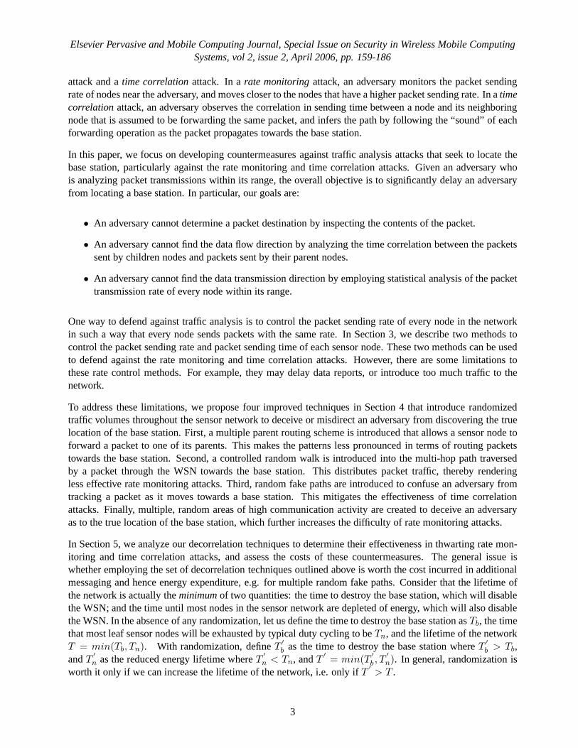
Figure 2: Decorrelating packet send times via random delays.

3.2 Decorrelating Packet Sending Times

Packet encryption can hide a packet destination, but cannothide its sender. By carefully monitoring the packetsending time of every node, an adversary may obtain some information about data traffic flows. For example,if a parent nodes receives a packet from its child nodec and forwards that packet immediately, an adversarycan observe the short time interval betweens and c and eventually infer the parent-child hierarchy givensufficiently long observations.

To prevent this, we decorrelate the packet sending times between a parent node and its child nodes. Here weonly consider the situation that every node sends data at thesame rate. This situation occurs when every noderegularly aggregates data from its children nodes and sendsa result to its parent node. Suppose all child nodesand parent nodes report their data during time periodT . Let’s denote the time interval between two childnodes sending packets as∆tc (we assume sensor nodes use a MAC layer protocol to avoid packet collisions),the time interval from the last child node sending data to theparent node sending data as∆tp, and the timebetween a parent node sending data and its grandparent forwarding data as∆tr. We denote∆tc, ∆tp, ∆tras the average value of∆tc, ∆tp, and∆tr. If the differences between∆tc, ∆tp and∆tr are observable, anadversary may be able to extract which node is the parent nodeafter monitoring the network for an extendedperiod of time.

If the parent node and child nodes send packets with the same rate, sensor nodes can introduce random delaybetween packet sending times. This makes the differences between∆tc, ∆tp and∆tr unobservable. To dothis, first the time periodT is divided intom slots, if there arem − 1 child nodes and 1 parent node. Everynode is assigned a slot and randomly chooses a time within itsslot to send its packet. For example, in Figure 2,the time slot assignment algorithm is centered at the parentnode. The parent node informs each child node ofits time slot with a secure unicast message. Nodesn1 to n4 aren5’s child nodes, andn6 is n5’s parent node.Figure 2(a) shows every node sends its packet as soon as it can. The differences between∆tc, ∆tp and∆trare correlated. Figure 2(b) shows thatn1 to n5 occupy different time slots and each node sends its packetrandomly within its time slot. The differences between∆tc, ∆tp and∆tr are indistinguishable. Experimentsshow that a sensor node only spends about 40 to 50 milliseconds to send a 36-byte packet. Normally, a sensorreports data once per minute or once per tens of seconds. In a connected sensor network, a sensor node mayhave 10 to 20 neighboring nodes. So the time slot is big enoughfor a sensor node to successfully send itspacket.

6


n5n5

n6n6

(a)

(b)

(c)

n5

n6

ID5||KC5(P2)

ID1||KC1(P1) ID2||KC2(P2) ID1||KC1(P1) ID2||KC2(dummy)

n1 n2 n2n2 n1n1

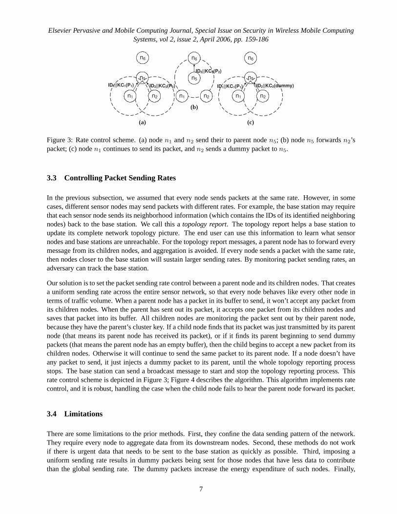
Figure 3: Rate control scheme. (a) noden1 andn2 send their to parent noden5; (b) noden5 forwardsn2’spacket; (c) noden1 continues to send its packet, andn2 sends a dummy packet ton5.

3.3 Controlling Packet Sending Rates

In the previous subsection, we assumed that every node sendspackets at the same rate. However, in somecases, different sensor nodes may send packets with different rates. For example, the base station may requirethat each sensor node sends its neighborhood information (which contains the IDs of its identified neighboringnodes) back to the base station. We call this atopology report. The topology report helps a base station toupdate its complete network topology picture. The end user can use this information to learn what sensornodes and base stations are unreachable. For the topology report messages, a parent node has to forward everymessage from its children nodes, and aggregation is avoided. If every node sends a packet with the same rate,then nodes closer to the base station will sustain larger sending rates. By monitoring packet sending rates, anadversary can track the base station.

Our solution is to set the packet sending rate control between a parent node and its children nodes. That createsa uniform sending rate across the entire sensor network, so that every node behaves like every other node interms of traffic volume. When a parent node has a packet in its buffer to send, it won’t accept any packet fromits children nodes. When the parent has sent out its packet, it accepts one packet from its children nodes andsaves that packet into its buffer. All children nodes are monitoring the packet sent out by their parent node,because they have the parent’s cluster key. If a child node finds that its packet was just transmitted by its parentnode (that means its parent node has received its packet), orif it finds its parent beginning to send dummypackets (that means the parent node has an empty buffer), then the child begins to accept a new packet from itschildren nodes. Otherwise it will continue to send the same packet to its parent node. If a node doesn’t haveany packet to send, it just injects a dummy packet to its parent, until the whole topology reporting processstops. The base station can send a broadcast message to startand stop the topology reporting process. Thisrate control scheme is depicted in Figure 3; Figure 4 describes the algorithm. This algorithm implements ratecontrol, and it is robust, handling the case when the child node fails to hear the parent node forward its packet.

3.4 Limitations

There are some limitations to the prior methods. First, theyconfine the data sending pattern of the network.They require every node to aggregate data from its downstream nodes. Second, these methods do not workif there is urgent data that needs to be sent to the base station as quickly as possible. Third, imposing auniform sending rate results in dummy packets being sent forthose nodes that have less data to contributethan the global sending rate. The dummy packets increase theenergy expenditure of such nodes. Finally,

7


while (1){sendPs to parent nodelisten to packet sending of neighboring nodesif receive packetpif (p.sender == parent node) {

if ((p == Ps)||(p == dummy)){Ps ← dummy}} else if (p.sender ∈ s.children) {

if (p 6= dummy&&Ps == dummy) {Ps ← p}}wait for next time slot}

Figure 4: Algorithm for packet sending control. (Ps is the packet to send)

( a ) shortest path routing

( c ) multi-parent routing+random

walk

( d) multi-parent routing+random

walk + fractal propagation

base station base station base station

sensor node

sensor node

sensor node

( b ) multi-parent routing

base station

sensor node

Figure 5: Techniques to counter traffic analysis.

they introduce extra delays in forwarding packets at each hop, cumulatively increasing the time to deliver datafrom source nodes to the base station. In the next section, weintroduce more advanced schemes to defendagainst traffic analysis attacks.

4 Inhibiting Traffic Analysis Attacks With Randomized Traffi c

This section introduces a suite of randomized network traffic techniques that improve upon Section 3’s basictraffic analysis countermeasures. These techniques do not impose onerous limitations such as a high uniformsending rate throughout the network or enforced aggregation at every hop, as in the previous section. Figure 5summarizes each of the major randomization techniques thatwe introduce in this section.

8


base station

v2 (x)

v3 (x+1)

v4 (x+1)

v5 (x)

u (x)

v6 (x − 1)

v1 (x−1)

��

Figure 6: Neighbors and parents of nodeu. Figure shows node ID and itslevel value. In SP, nodeu hasone parent nodev1. In MPR, nodeu has two parent nodes,v1 andv6. In RW, u forwards packets tov1 withprobabilitypr or v6 with probability1− pr.

4.1 Multi-parent routing scheme

To reduce the starkness of pronounced paths caused by shortest path (SP) routing, as shown by the directnode-to-base station route in Figure 5(a), we require each node to randomly select one of multiple parentnodes to route data to the base station, as shown in Figure 5(b). When a node needs to forward a packet, thenode randomly selects one of its parent nodes to forward the packet. We call this scheme multi-parent routing(MPR). We propose two methods for setting up multiple parents for each node. In the first method, as shownin Figure 6, whenever a base station sets up a routing structure, it broadcasts or floods a message called thebeacon. The beacon message contains alevelfield. The base station sets the value oflevel to 0. When a nodeforwards a beacon message, it increments it by 1. So the valueof level represents the number of hops that anode is from the base station along a particular path. A sensor nodes selects all neighboring nodes whoselevelvalue is less thans’s levelvalue as its parent nodes. In the second method, a node monitors all beaconmessages it receives before forwarding the first beacon message. Since a nodes has to wait for some amountof time before forwarding a beacon message (waiting time in MAC layer), it selects all nodes from whom itreceives a beacon message while waiting to forward the first received beacon message as its parent nodes.

An adversary has several ways to attack these multi-parent routing setup schemes. For example, a maliciousnode can claim a lowlevelvalue to attract traffic from other nodes, or it can use unfairmedia access controlmechanisms to occupy the wireless channel. Protecting routing schemes from such attacks is beyond the scopeof this paper. Here we assume that the routing set up scheme isrelatively fast, so an adversary doesn’t haveenough time to attack the routing set up process. Several mechanisms [13, 5] have already been proposed toprotect against attacks during the routing setup. Notice that thelevel information will be erased by every nodeafter the routing paths are set up. So even if a node is compromised, an adversary won’t know the distance tothe base station because thelevel information of the compromised node won’t be available.

4.2 Random Walk

To further diversify routing paths and mitigate rate monitoring attacks, we propose a random walk (RW)routing scheme. In RW, when a node receives a packet, it forwards the packet to one of its parent nodeswith probabilitypr. However, it uses a random forwarding algorithm with probability 1 − pr. In the randomforwarding algorithm, the node forwards the packet to one ofits neighboring nodes with equal probability.Like [12] and [23], MPR and RW use probabilistic routing. However, [12] and [23] use probabilistic routingfor reliable data transmission in sensor networks, while weuse probabilistic routing to defend against theratemonitoring attack.

9


The RW technique results in some packets traversing a longerpath to reach the base station than the shortestavailable path, as shown in Figure 5(c). This implies that RWwill consume more energy per node on anaverage. To estimate how much extra energy is consumed by RW,we calculate the cost C of RW, where costis defined as [5]:C = M ′

M. Here,M ′ is the average number of hops a packet takes to reach the base station

from an aggregator node in RW, andM is the number of hops a packet takes to reach the base station fromthe same aggregator node in SP. Clearly,M ′ depends on the several factors related to network topology,e.g.how many neighbors a sensor node has, how far the base stationis from a sensor node or from one of itsneighboring nodes, and so on. We calculate the value ofC by making the following simplifying assumption.Suppose a nodeu randomly selects a neighboring nodev to forward a packet, and the distance (number ofhops along the shortest path) betweenv and the base station isd, while the distance betweenu and base stationis d′. We assume that the probability thatd > d′ is the same as the probability thatd < d′. So on average,whenu forwards a packet tov, the distance from the base station doesn’t change. Only when u forwards thepacket to its parent node, the distance is reduced by 1. We denoten as the number of hops from the aggregatorto the base station in SP, andn′ as the number of average hops in RW. We haven′×pr = n. This impliesC = M ′

M= 1

pr.

In addition, a packet will take a longer time to reach the basestation in RW. In fact, the extra time delayis directly proportional (linear) to the extra hops used forforwarding the packet. So, the time cost for eachpacket to reach the base station is roughly1

prin RW.

4.3 Fractal Propagation

MPR and RW spread out data traffic and make it difficult to use a rate monitoring attack. However, RW is stillvulnerable to thetime correlationattack. Usually, for a nodes, the number of parent nodes is less than halfof s’s neighboring nodes, and for energy and efficiency considerations,pr > 0.5 typically. As a result, thepossibility that a node forwards a packet to its parent node is higher than the possibility it forwards the packetto any one of its other neighbors. An adversary can exploit this to launch a time correlation attack, either byinjecting abnormal report data or monitoring over a long period of time.

To address the shortcomings of MPR and RW, we propose a new technique calledfractal propagation. Inthis technique, severalfakepackets are created and propagated in the network to introduce more randomnessin the communication pattern. When a node hears that its neighboring node is forwarding a packet to thebase station, the node generates a fake packet with probability pc, and forwards it to one of its neighboringnodes. To control the propagation range of the fake packet, each newly generated fake packet contains alengthparameter with valueK. K is a constant that is known to all nodes, so an adversary cannot flood the wholenetwork by sending fake packets withlengthparameter higher thanK. When a node receives a fake packet,it decrementslengthby 1. If the value oflengthis greater than zero, the node forwards the fake packet to oneof its neighboring nodes (not necessarily in the direction of the base station). If the value oflengthis zero, anode stops forwarding the fake packet. In addition, when a node hears that its neighboring node is forwardinga fake packet to someone else withlengthvaluek (k < K), it generates and forwards another fake packetwith probabilitypc andlengthvaluek − 1.

These fake packets spread out in the network and their transmission paths form a tree (see Figure 5(d)). Inparticular, the communication traffic is much more spread out than RW. So even if an adversary can track apacket using time-correlation, she cannot track where the real (as opposed to fake) packet is going. This isbecause she cannot differentiate between a real and a fake packet without knowing the encryption key.

Suppose a node hasx neighboring nodes on average. Letpf = pc×x andf(K) represents the total length of

10


a fake tree that originated withlengthvalueK. We have

f(K) = pf×f(K − 1) + f(K − 1) + 1

Solving this recursive equation, we get

f(K) =K−1∑

i=0

(pf + 1)i =

{

(pf+1)K−1

pfif pf > 0

K otherwise

Suppose the length of real path from the aggregator node to the base station isn. The cost is

C =M ′

M=

n + n×pf×f(K)

n=

n + n× pf × (pf +1)K−1

pf

n= (pf + 1)K

If we combine RW and the fractal idea, the total cost is

C =(pf + 1)K

pr

If we use fixed values ofpr, pf andK, the average cost is a fixed value that is independent of the size of thenetwork.

4.3.1 Fractal propagation with different forking probabil ities

One problem with simple fractal propagation is that it generates a large amount of traffic near the base station.This will potentially increase the packet collision rate and packet loss rate.

To address this problem, nodes can use different probabilities to generate fake packets. When a node forwardspackets more frequently, it sets a lower probability for creating new fake packets. This technique is calledDifferential Fractal Propagation (DFP). The algorithm forsetting this probability is as follows. When thepacket forwarding rater at a node is lower than a thresholdh, the node generates new fake packets withprobability p. When the packet forwarding rate is higher thanh, the node generates new fake packets withprobabilityp′ = p×(h/r)2; h can be chosen as the packet sending rate of the aggregator node.

4.3.2 Enforced fractal propagation

The idea of fractal propagation aids significantly in spreading out the communication traffic evenly over thenetwork and obfuscating any paths to the base station. To make matters worse for an adversary, we generatelocal high data sending rate areas, calledhot spots, in the network. An adversary may be trapped in those areasand not be able to determine the correct path to the base station. This routing technique is called DifferentialEnforced Fractal Propagation (DEFP). The challenge here ishow to create hot spots that are evenly spread

11


ID Ticketsforward

probability

v1

v2

v3

v4

v5

v6

1

1

1

1

1

1

1/6

1/6

1/6

1/6

1/6

1/6

v3

v5

u

v1

v2

v4

v6

Ticket table of node u

v3

v5

u

v1

v2

v4

v6

Ticket table of node u

ID Ticketsforward

probability

v1

v2

v3

v4

v5

v6

1

5

1

1

1

1

1/10

1/10

1/2

1/10

1/10

1/10

(a) before nodeu forwards any fake packet (b) afteru forwards a fake packet to nodev3

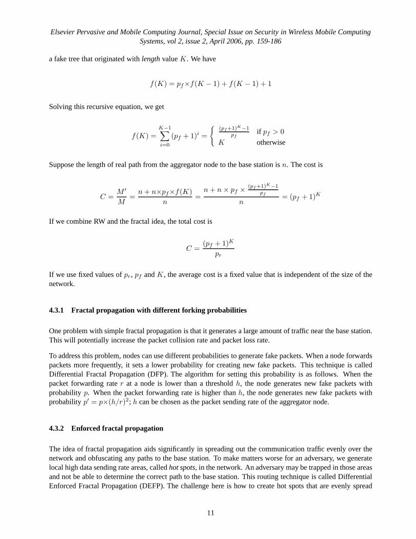
Figure 7: Ticket table of nodeu

out in the network, such that only a minimum (preferably zero) amount of extra communication/coordinationamong the sensor nodes is needed.

DEFP is a simple distributed algorithm based on DFP. The key idea is to let the nodes that forwarded fakepackets earlier have a higher chance to forward fake packetsin the future. In particular, if a nodeu forwardeda fake packet to another nodev in the past, then it forwards the next fake packet received tov with a higherprobability. The node uses alottery schedulingalgorithm [22] to choose the next node to forward the fakepacket to. In this algorithm (see Figure 7), a node assigns tickets to each of its neighboring nodes. It choosesthe next node to forward a fake packet to based on the number oftickets assigned to the neighboring nodes. Aneighboring node with more tickets assigned has the higher probability of being chosen. In the beginning, allneighboring nodes are assigned one ticket. When the node chooses a neighboring node as the next node forforwarding a fake packet, it increments that node’s ticketsby k. This way, after a node has forwarded a fakepacket to one of its neighboring nodes, it will continue to forward other fake packets to the same neighboringnode with higher and higher probability. If an area of nodes receive fake packets, they are more likely toprocess more and more fake packets in the future. This will turn that area into a hot spot. It is also very easyto destroy current hot spots and reconstruct new hot spots atdifferent places. For example, sensor nodes justreset the value of tickets to 1 when they receive a broadcast message from the base station, and then start tobuild hot spots from scratch. A patient attacker can wait at ahot spot until the communication pattern changes.While this will allow the attacker to determine that he was ata fake hot spot, it does not provide any otherinformation about the possible location of the base station. Furthermore, waiting for a long time at a fake hotspot will add more delay to finding the location of the base station.

4.4 Node Compromises

If an adversary compromises a node, she can normally find out the identity of its parent nodes, and read thecontents of all packets passing through this node. In addition, by monitoring the traffic for some sufficientlylong period of time, she can obtain distribution information about all the ancestor nodes within her activityrange. However, with this knowledge, she cannot determine the location of the base station, and cannot blockcommunication between an aggregator node and the base station. To determine the location of the base station,the adversary will have to compromise a large number of nodesalong the path to the base station.

To further minimize the damage of node compromise, we propose thedirectional pairwise IDmechanismsuch that every node has different IDs to its children nodes and parent nodes. When a nodeu is compromised,an adversary knows its parent nodep’s ID. However, the parentp only uses that ID to accept packets, anddoesn’t use that ID to send packets. So the adversary cannot know which node isp by listening to packets.

12


Hops Average Number of Compromised Nodes5 53.7

10 87.115 120.820 152.625 181.2

Table 1: Average number of nodes that need to be compromised to trace back to the base station givendirectional pairwise ID’s.

She has to compromiseu’s neighboring nodes one by one, until capturingp.

Concretely, every node shares a unique pair of IDs with each of its parent nodes. For example, suppose nodeu has parent nodep1 andp2. Thenu has an IDIDup1

to p1, andp1 has an IDIDp1u to u. Thusu andp2

shares another pair of IDsIDup2andIDp2u. Whenu sends a packet top1, it uses the format that

IDup1||EKCu(type||IDp1u||data)

If u is compromised, the adversary knowsKCu, IDup1andIDp1u, but she doesn’t knowp1’s IDs to p1’s

parent nodes. She has to compromiseu’s neighboring nodes which are notu’s children nodes, until shecapturesp1. This mechanism increases the workload of node compromise.Table 1 shows the averagenumber of nodes that need to be compromised in a random distributed network under a single parent routingscheme. We can see that if the first compromised node is 15 hopsaway from the base station, the adversaryneeds to compromise about 120 other nodes, instead of 15 nodes, to get to the base station. This shows that anadversary has to compromise a relatively large number of nodes along the path until reaching the base station.

In fractal propagation, if an adversary compromises a node,she can find out whether a packet is a fake orreal. However, she cannot obtain any information other thanwhat was discussed above. The adversary canattempt to launch a DoS attack by generating several fake packets and forwarding them to flood the network.However, the propagation area of a fake packet is limited by the value of thelengthparameter. A fake packetcan propagate and generate new fake packets only within a small part of the network, so the damage due tosuch DoS attacks is limited to a small part of the network.

Cooperating adversaries can launch a collaborative attack. For example, two cooperating adversaries ondifferent sides of a WSN can respectively determine the direction (a vector) where a base station is possiblylocated from their current location by analyzing packets over just a few hops. They can then form an estimateof the base station’s location by intersecting the two vectors. However, such an attack requires that thedirection in which a parent node is located is precisely the direction towards the base station. This is quiteunlikely in a randomly distributed sensor network. In addition, MPR increases the difficulty in determiningthe precise geographic direction towards the base station,forcing the adversary to compromise a large numberof nodes.

Finally, an adversary can also generate several forged datapackets and forward them to the base station inan attempt to flood the base station. However, mechanisms currently exist that allow intermediate nodes tofilter out forged data packets, e.g. see [24, 26]. In these mechanisms, intermediate nodes use randomly pre-distributed pair-wise keys to verify the authenticity of the data sent by the aggregator node. Forged packetsare filtered out by each intermediate node with a certain probability and thus prevented from propagating overa long path.

13


10 20 30 40 50 60 70 80

10

20

30

40

50

60

70

80

40

120

180

10 20 30 40 50 60 70 80

10

20

30

40

50

60

70

80

40

90

350

hot spot

(a) RW. (b) Naive fractal propagation.

10 20 30 40 50 60 70 80

10

20

30

40

50

60

70

80

40

60

120

10 20 30 40 50 60 70 80

10

20

30

40

50

60

70

80

40

70

140

hot spots

(c) DFP. (d) DEFP.

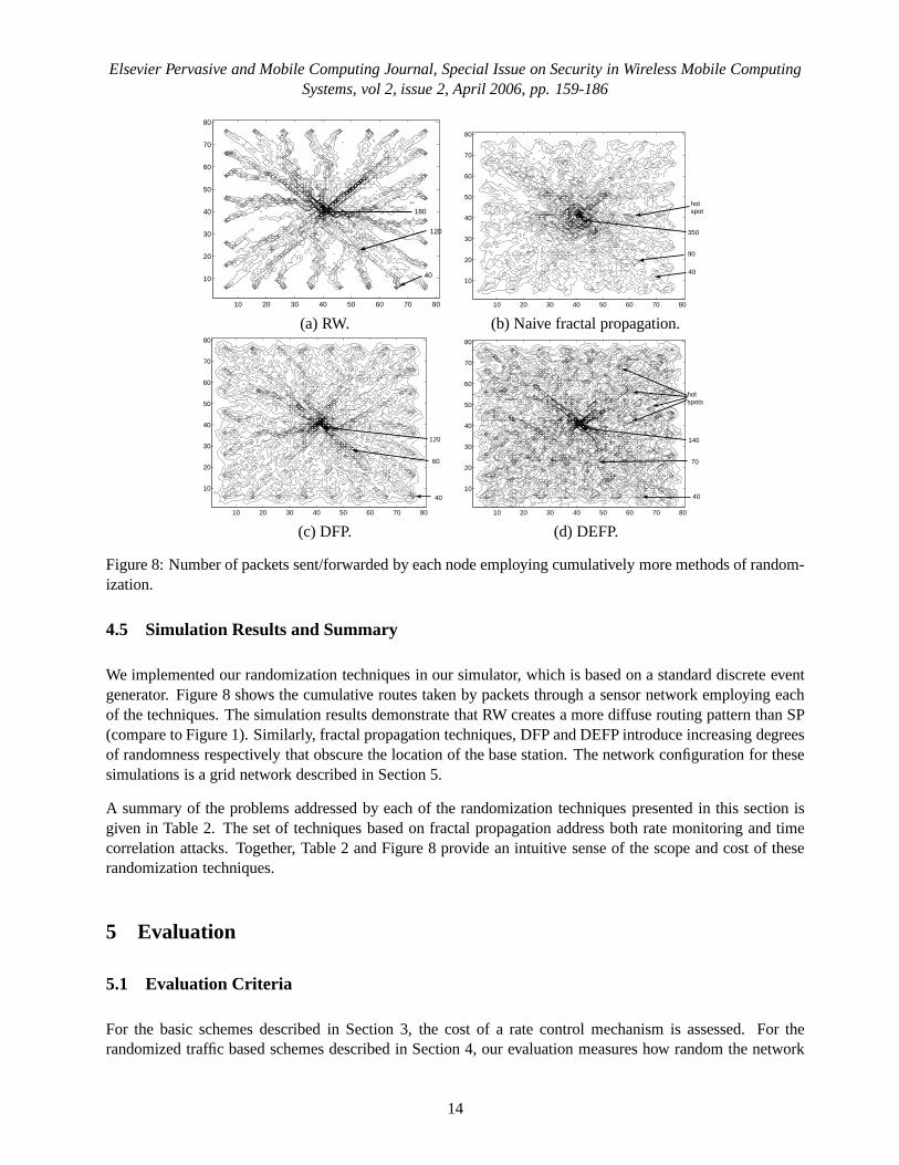
Figure 8: Number of packets sent/forwarded by each node employing cumulatively more methods of random-ization.

4.5 Simulation Results and Summary

We implemented our randomization techniques in our simulator, which is based on a standard discrete eventgenerator. Figure 8 shows the cumulative routes taken by packets through a sensor network employing eachof the techniques. The simulation results demonstrate thatRW creates a more diffuse routing pattern than SP(compare to Figure 1). Similarly, fractal propagation techniques, DFP and DEFP introduce increasing degreesof randomness respectively that obscure the location of thebase station. The network configuration for thesesimulations is a grid network described in Section 5.

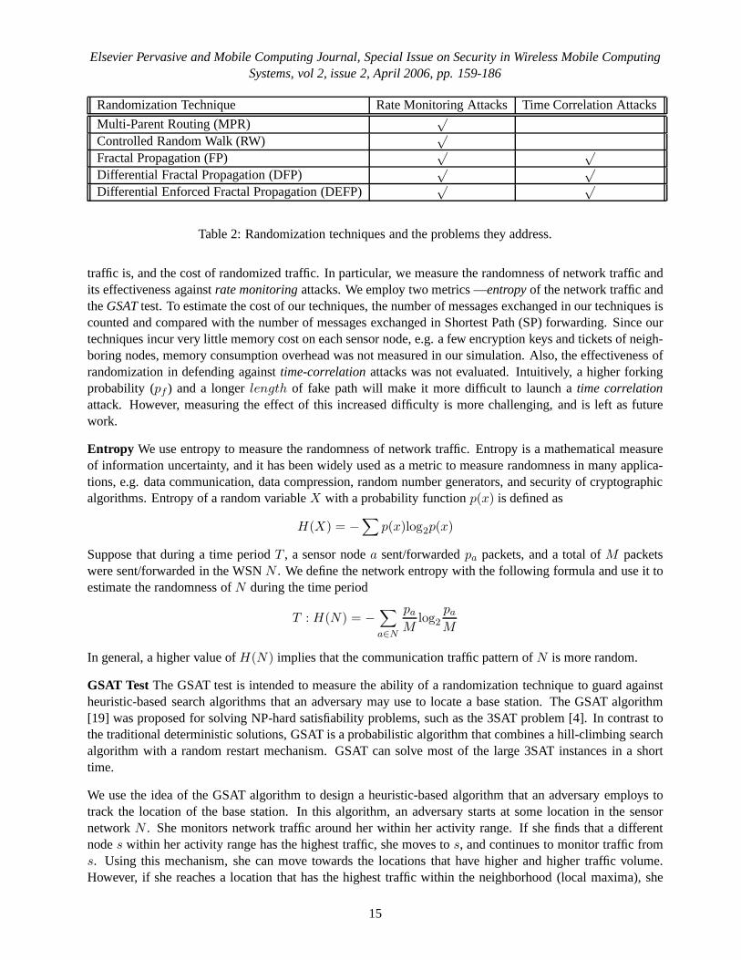
A summary of the problems addressed by each of the randomization techniques presented in this section isgiven in Table 2. The set of techniques based on fractal propagation address both rate monitoring and timecorrelation attacks. Together, Table 2 and Figure 8 providean intuitive sense of the scope and cost of theserandomization techniques.

5 Evaluation

5.1 Evaluation Criteria

For the basic schemes described in Section 3, the cost of a rate control mechanism is assessed. For therandomized traffic based schemes described in Section 4, ourevaluation measures how random the network

14


Randomization Technique Rate Monitoring Attacks Time Correlation Attacks

Multi-Parent Routing (MPR)√

Controlled Random Walk (RW)√

Fractal Propagation (FP)√ √

Differential Fractal Propagation (DFP)√ √

Differential Enforced Fractal Propagation (DEFP)√ √

Table 2: Randomization techniques and the problems they address.

traffic is, and the cost of randomized traffic. In particular,we measure the randomness of network traffic andits effectiveness againstrate monitoringattacks. We employ two metrics —entropyof the network traffic andtheGSATtest. To estimate the cost of our techniques, the number of messages exchanged in our techniques iscounted and compared with the number of messages exchanged in Shortest Path (SP) forwarding. Since ourtechniques incur very little memory cost on each sensor node, e.g. a few encryption keys and tickets of neigh-boring nodes, memory consumption overhead was not measuredin our simulation. Also, the effectiveness ofrandomization in defending againsttime-correlationattacks was not evaluated. Intuitively, a higher forkingprobability (pf ) and a longerlength of fake path will make it more difficult to launch atime correlationattack. However, measuring the effect of this increased difficulty is more challenging, and is left as futurework.

Entropy We use entropy to measure the randomness of network traffic. Entropy is a mathematical measureof information uncertainty, and it has been widely used as a metric to measure randomness in many applica-tions, e.g. data communication, data compression, random number generators, and security of cryptographicalgorithms. Entropy of a random variableX with a probability functionp(x) is defined as

H(X) = −∑

p(x)log2p(x)

Suppose that during a time periodT , a sensor nodea sent/forwardedpa packets, and a total ofM packetswere sent/forwarded in the WSNN . We define the network entropy with the following formula anduse it toestimate the randomness ofN during the time period

T : H(N) = −∑

a∈N

pa

Mlog2

pa

M

In general, a higher value ofH(N) implies that the communication traffic pattern ofN is more random.

GSAT Test The GSAT test is intended to measure the ability of a randomization technique to guard againstheuristic-based search algorithms that an adversary may use to locate a base station. The GSAT algorithm[19] was proposed for solving NP-hard satisfiability problems, such as the 3SAT problem [4]. In contrast tothe traditional deterministic solutions, GSAT is a probabilistic algorithm that combines a hill-climbing searchalgorithm with a random restart mechanism. GSAT can solve most of the large 3SAT instances in a shorttime.

We use the idea of the GSAT algorithm to design a heuristic-based algorithm that an adversary employs totrack the location of the base station. In this algorithm, anadversary starts at some location in the sensornetworkN . She monitors network traffic around her within her activityrange. If she finds that a differentnodes within her activity range has the highest traffic, she moves to s, and continues to monitor traffic froms. Using this mechanism, she can move towards the locations that have higher and higher traffic volume.However, if she reaches a location that has the highest traffic within the neighborhood (local maxima), she

15


Size Average # Number of SendingNeighbors Aggregators Rate

Grid 81×81 8 28 4/minuteRandom 4500 20 28 4/minute

Table 3: Network configuration Parameters

selects a direction at random, moves in that direction for some time, and then repeats the above algorithm.She continues to do this until she finds the base station.

The GSAT test measures the average number of hops an adversary takes to finally reach the base station usingthis heuristic algorithm. A large value of the GSAT test implies that the routing technique has better potentialto guard against heuristic-based search algorithms that anadversary may employ to locate a base station.

In addition to the degree of randomness, the exact values of entropy and the GSAT test depend on several othernetwork characteristics, e.g. network structure, networksize, number and location of aggregator nodes. Toevaluate our techniques, we have focused on differences in entropy and GSAT test values measured under thecases when one of the proposed traffic analysis countermeasures is used and the case when no traffic analysisdefenses are used. We also experimented with different values ofPr in RW andPf in DEFP, to understandthe effects of these parameters. We simulated two network structures in our experiments: a grid topology anda random topology. Table 3 shows the parameters used in our simulation. Aggregators are located at the fouredges of the network.

5.2 Message Overhead of Rate Control Mechanism

2

4

6

8

10

12

14

16

200 400 600 800 1000 1200 1400 1600 1800 2000

M’/M

Nodes

(a) Rate Control Message Cost

sparsemiddledense

1

1.01

1.02

1.03

1.04

1.05

1.06

1.07

1.08

0 5 10 15 20 25 30

M’/M

days

(b) Integrated Message Overhead

500 nodes1000 nodes2000 nodes

Figure 9: Overhead of uniform rate control countermeasuresto traffic analysis.

We defineC = M ′

Mto measure the data transmission overhead of our basic suiteof traffic analysis countermea-

sures, whereC is the cost measurement,M is the number of messages without basic traffic analysis defenses,andM ′ is the number of messages with the our basic traffic analysis countermeasures. In this experiment, wesimulated and measured the message overhead of the rate control scheme, since it introduces extra “dummy”packets. We ran three groups of tests. For each group of tests, we employed a different network topology.These networks differed from one another in the number of nodes, but had the same node density. The numberof nodes varied from 250 to 2000. For each test, sensor nodes were randomly deployed in the network area.

16


Entropy Traffic Center Traffic(SP) (BR) (SP) (BR) (SP) (BR)

Grid 9.64 11.40 39000 7×106 10080 4×105

Random 8.20 12.08 21000 5×106 2792 1.8×105

Table 4: Entropy and number of messages exchanged in SP and BR. (Traffic means the total messages ex-changed in the network, and Center Traffic means the number ofmessages exchanged in the close vicinity ofthe base station.)

We set up routing, and measuredM ′ andM . For the same number of nodes with the same network density,we repeated the test 50 times and calculated the average value. Figure 9 (a) shows the simulation result ofM ′

M

for three different network densities. We can see that the overhead of our rate control strategy increases as thesize of the network increases. Our initial analysis and experiments show thatM

′

M∝√

N , whereN is the size(number of nodes) of the network. That means the rate controloverhead is not scaling directly with the sizeof the network.

However, if topology information is not required frequently, the overhead of the rate control scheme onlyoccupies a small part of the total cost. The network traffic isdominated by regular sensed data report, whoseanti-traffic message overhead is 1. Figure 9 (b) shows the total message overhead combining sensor datapackets and topology reports over an intermediate density network. We assume that every node reports itsdata once per minute, and the base station requires a topology report every one to thirty days. Figure 9(b) shows that the total overhead reduces as the base stationrequires topology reports less frequently. Forexample, if the topology report is performed once a week, total overhead is less than 1.01. In this context, theoverhead of sending “dummy” packets is much less noticeable.

5.3 Effectiveness and Cost of Randomized Traffic Techniques

To evaluate the effectiveness of our randomized traffic countermeasures, we simulated them over a grid net-work (see Table 3) and measured the values of entropy, GSAT test, and energy cost (number of messages ex-changed). We simulated the following techniques: MPR, MPR+RW, MPR+RW+DFP, and MPR+RW+DEFP.For simplicity, we use MPR, RW, DFP, and DEFP respectively torefer to these techniques in the rest of thepaper. In these simulations, we setpr to 0.6,pf to 0.2, andK to 6.

To obtain an estimate of an upper bound of entropy and GSAT values, and a lower bound on the cost, wesimulated two routing mechanisms. The first routing mechanism is SP, which selects the shortest path to thebase station from each sensor node. SP provides a measure of lower bound on the cost of routing, but resultsin very pronounced communication patters as shown in Figure1. The second routing mechanism is called thebroadcast scheme (BR scheme). In this mechanism, every message sent by an aggregator node is flooded tothe entire network. Since BR generates uniform network traffic, it provides a measure of an upper bound ofentropy and GSAT values. Table 4 shows the entropy values andnumber of messages exchanged in SP andBR.

Figure 10 (a) shows the entropy measured for various routingtechniques. All data reported here are an averageover 20 runs. As expected, entropy is lowest for SP and highest for broadcast. Entropy for MPR and RW ishigher than SP, but lower than DFP and DEFP, which confirms theprogression of increasing randomnessrevealed in Figure 8’s various subgraphs. Figure 10 (a) demonstrates that the idea of generating fake packets

17


7

8

9

10

11

12

SP MPR RW DFP DEFP broadcast

Ent

ropy

Algorithms

0

200

400

600

800

1000

SP MPR RW DFP DEFP broadcast

#of S

earc

h S

teps

Algorithms

3X35X59X9

(a) entropy (b) GSAT test: number of search steps

0

20000

40000

60000

80000

100000

120000

SP MRP RW DFP DEFP

#of M

essa

ges

Algorithms

messagesmessages in center area

(c) message cost

Figure 10: Effectiveness and cost of randomization countermeasures against traffic analysis.

in a controlled manner does aid in making the network traffic pattern more random. This is in addition to theoriginal goal of defending against time-correlation analysis.

To determine resiliency against a GSAT search, we simulatedthe data traffic and recorded the number ofpackets sent/forwarded by each node in a log file. We initialized a starting point for the adversary in thenetwork and used the GSAT algorithm to discover thebase station area. We recorded the number of steps theadversary takes to get into the base station area. For each log file, we set 81 different initial locations. Foreach initial location, we ran GSAT to search for the base station area for 100 times, and recorded the numberof hops the adversary takes to get into the base station area.Finally, we computed the average number of hopsthe adversary takes to get into the base station area for eachtechnique. In addition, we experimented withthree different activity ranges of the adversary: adversary could monitor data traffic over3×3, 5×5, and9×9areas around her respectively.

Figure 10 (b) shows the results of the GSAT test. First, we notice that randomization countermeasures signif-icantly increase the number of steps an adversary has to taketo locate the base station. The addition of eachtechnique increases the frustration of the adversary, withvarying degrees of effectiveness. For example, shecan discover the base station area in 34 steps in SP (activityrange3×3), and 653 steps in DEFP, which isabout 19 times more. Notice that the number of search steps needed when all packets are broadcast is onlyabout 1.5 times more than the number of steps needed in DEFP approach. In this sense, DEFP achieves closeto the maximum decorrelation upper bound represented by broadcast.

18


The activity range of an adversary also impacts the GSAT value. If the activity range is larger, the corre-sponding GSAT value is smaller. This implies that the adversary can find the base station in fewer hops. Evenwhen the activity range of the adversary is large (9×9), our traffic analysis defenses significantly increase thenumber of hops an adversary has to take to locate the base station area.

Also, we see that the GSAT values correlate with the entropy values shown in Figure 10 (a) (except DEFP).Higher entropy corresponds to a larger value of GSAT. This implies that both entropy and GSAT are usefulmetrics to measure the randomness in network traffic. The only exception is DEFP. Since DEFP convergessome traffic together to formhot spots, it results in less entropy compared to DFP. However, thosehot spotsmake it more difficult for an adversary to locate the base station using a GSAT search algorithm. This isevident from the higher values of GSAT in DEFP.

Figure 10 (c) shows the cost of randomization in terms of the total number of messages sent/forwarded byall nodes in the network, and the number of messages sent/forwarded by nodes near the base station (whichis an area of20×20 nodes with base station at center). The total traffic in RW is about 1.8 times larger thanthe total traffic in SP for the whole network and the area near the base station. The total message cost ofDFP and DEFP is about 2.8 times the message cost of SP in the whole network, and 2.4 times near the basestation. In our simulation, when aggregators send four packets per minute, the nodes directly connected tothe base station forward about 14 packets per minutes in SP, and about 34 packets per minute in DEFP. Thisis easily feasible in the current sensor network technology. An important point to note is that the messagecost of these algorithms is constant. It doesn’t increase with increasing network size. The final observationis that broadcast costs about 70 times more messaging than DEFP, i.e. Table 4 give7x106 as the number ofmessages for broadcasting in a grid while Figure 10 (c) givesabout105 as the number of messages for DEFP.The overhead messaging cost provides an indication of the energy cost to the WSN, since packet transmissioncosts over a thousand times more energy per bit than computation, but is not a precise equivalence due toother factors such as duty cycling and degree of computation.

The big picture emerging from Figure 10’s three graphs is that our most advanced randomization suite DEFP,equivalent to MPR+RW+DFP+DEFP, achieves nearly the best decorrelation capabilities afforded by broad-cast at a fraction of the cost.DEFP achieves close to broadcast flooding’s maximum decorrelation, withinabout 50% of the maximum number of GSAT search steps requiredof an adversary. Yet, DEFP’s overheadof a hundred thousand messages is 70 times less than pure broadcast’s overhead obtained from Table 4. Thishighlights the considerable advantage gained by employingour randomization algorithms.

5.4 Effectiveness ofpr and pf

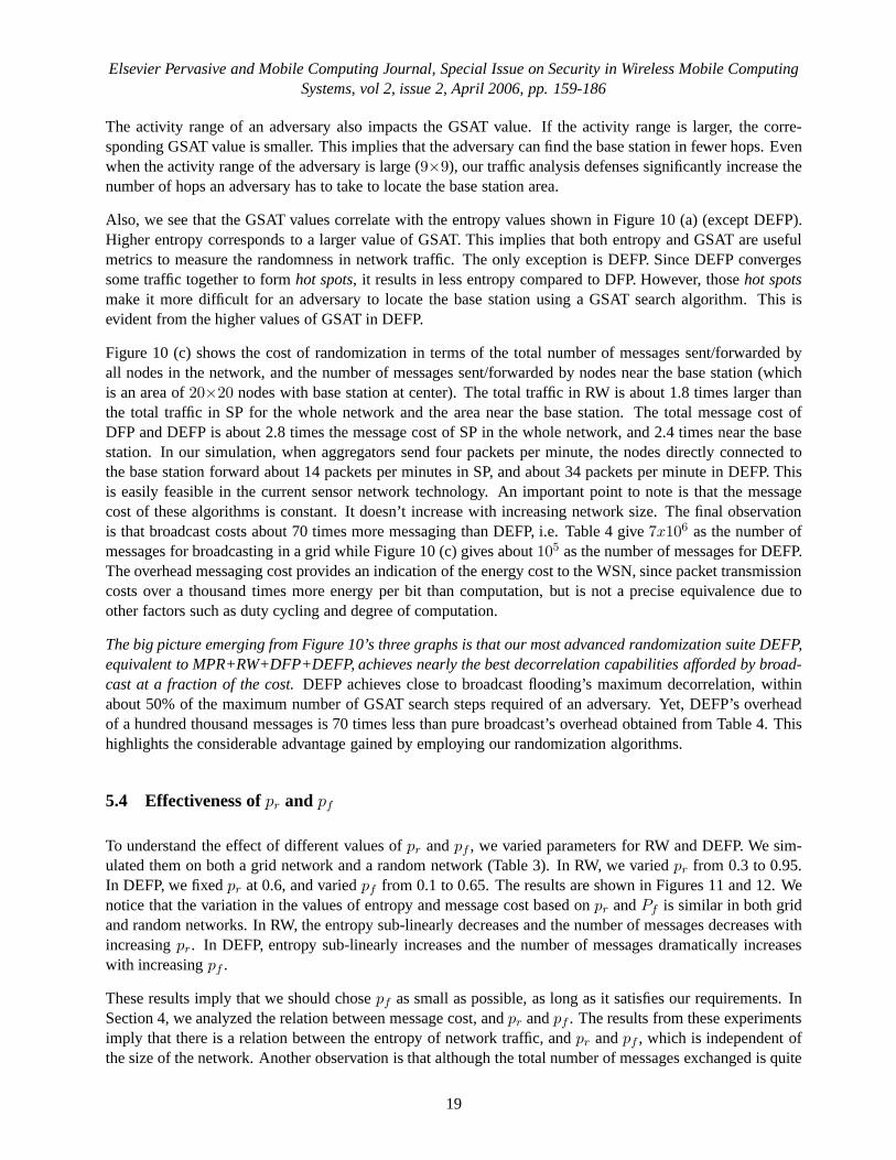
To understand the effect of different values ofpr andpf , we varied parameters for RW and DEFP. We sim-ulated them on both a grid network and a random network (Table3). In RW, we variedpr from 0.3 to 0.95.In DEFP, we fixedpr at 0.6, and variedpf from 0.1 to 0.65. The results are shown in Figures 11 and 12. Wenotice that the variation in the values of entropy and message cost based onpr andPf is similar in both gridand random networks. In RW, the entropy sub-linearly decreases and the number of messages decreases withincreasingpr. In DEFP, entropy sub-linearly increases and the number of messages dramatically increaseswith increasingpf .

These results imply that we should chosepf as small as possible, as long as it satisfies our requirements. InSection 4, we analyzed the relation between message cost, and pr andpf . The results from these experimentsimply that there is a relation between the entropy of networktraffic, andpr andpf , which is independent ofthe size of the network. Another observation is that although the total number of messages exchanged is quite

19


9.6

9.8

10

10.2

10.4

10.6

10.8

11

0.3 0.4 0.5 0.6 0.7 0.8 0.9

Ent

ropy

P_r

0

20000

40000

60000

80000

100000

120000

140000

160000

0.3 0.4 0.5 0.6 0.7 0.8 0.9

#of P

acke

ts

P_r

Total packetsPackets in base station area

(a) Entropy (RW) (b) Message overhead (RW)

10.75

10.8

10.85

10.9

10.95

11

11.05

11.1

11.15

11.2

11.25

0.1 0.2 0.3 0.4 0.5 0.6

Ent

ropy

P_f

0

50000

100000

150000

200000

250000

300000

0.1 0.2 0.3 0.4 0.5 0.6

#of P

acke

ts

P_f


(c) Entropy (DEFP) (d) Message overhead (DEFP)

Figure 11: Effectiveness and cost as a function ofpr (a)-(b) andpf (c)-(d) for a grid network.

large for very large values ofpf , the number of messages exchanged near the base station doesn’t change alot. This shows that the traffic control mechanism proposed in DFP and DEFP works quite well.

6 Related Work

Research in security issues in sensor networks has receivedmuch attention recently, e.g. secure data commu-nication [16], secure routing [13, 11, 5], secure data aggregation [18], and pairwise key setup [8, 3, 7, 14, 25].In the area of privacy in E-commerce, many techniques have been developed to protect the anonymity ofmessage senders and receivers. Our anti-traffic analysis techniques are similar to the methods used in tra-ditional privacy and anonymity research, but we have three unique properties: First, we focus on hiding thephysical location of a base station, instead of hiding the identity of a message sender or receiver. Second,the communication pattern in sensor networks is highly asymmetric and converges on a base station. Thismake it more difficult to protect the base station against traffic analysis attacks. Third, traditional networksare resource-rich compared to a WSN, and so the techniques developed for traditional networks cannot bedirectly used in sensor networks.

In traditional privacy research, mist routing requires pre-deployed, hierarchical and trusted routers [2]. [10]requires that every node can talk to every other node. The Onion routing protocol [9] disguises who talks to

20


9

9.5

10

10.5

11

11.5

12

0.3 0.4 0.5 0.6 0.7 0.8 0.9

Ent

ropy

P_r

0

10000

20000

30000

40000

50000

60000

70000

80000

90000

100000

0.3 0.4 0.5 0.6 0.7 0.8 0.9

#of P

acke

ts

P_r

Total PacketsPackets in base station area

(a) Entropy (RW) (b) Message overhead (RW)

11.4

11.45

11.5

11.55

11.6

11.65

11.7

11.75

11.8

11.85

11.9

0.1 0.2 0.3 0.4 0.5 0.6

Ent

ropy

P_f

0

50000

100000

150000

200000

250000

0.1 0.2 0.3 0.4 0.5 0.6

#of P

acke

ts

P_f


(c) Entropy (DEFP) (d) Message overhead (DEFP)

Figure 12: Effectiveness and cost as a function ofpr (a)-(b) andpf (c)-(d) for a random network.

whom on the Internet by layered encryption and by forwardingreceived messages in a random order. In addi-tion, a large number of messages are stored before forwarding them in a different order. A sensor node doesn’thave enough memory to store many packets. Thek-anonymous message transmission protocol proposed in[1] protects anonymity for both sender and receiver with lowdata transmission latency. Unfortunately, itshigh communication and computational requirements prevent it from being used in sensor networks. Thetechniques to disguise a receiver by routing each message tomultiple receivers using a multicast mechanismare proposed in [17, 20]. Tor [6] is the second-generation onion router, which is a circuit-based low-latencyanonymous communication service on the Internet. However,it needs to set up a large number of directoryservers, which is difficult to envision in sensor networks.

Recently, techniques to randomize communications during the network setup phase to protect the anonymityof the sensor network infrastructure were proposed in [21].In contrast, we focus on defending againsttraffic analysis during the data sending phase. In addition,we propose a more robust adversary model, andassume that an adversary can launch active attacks such as injecting traffic in the network, and compromisingsensor nodes. Preserving source-location privacy in WSNs was proposed by C. Ozturket.al. [15]. Thiswork proposes randomization techniques such as fake packets, persistent fake sources, and a random walk tohide the location of the source of data packet from discovery. Unlike our approach, fake packets are alwaysflooded, which incurs a high overhead cost. The key advantageof our approach is that it achieves much of thedecorrelative effects of flooding at a fraction of the cost. Also, our focus is on the arguably more difficult taskof hiding thedestinationof a data packet, i.e. base station, from discovery, since the patterns produced by the

21


tree-structured routing are quite pronounced and difficultto hide.

7 Future Work

There are a variety of research directions that could be morefully explored in the future. First, our workconsiders only one form of search algorithm, namely the GSATsearch. More advanced search techniquescould be evaluated. Second, the paper also has not developeda metric for evaluating the effectiveness ofour proposed techniques against time correlation attacks.The fractal propagation approach makes it moredifficult to trace a packet by inspecting transmission timesof adjacent nodes, because the attacker may windup following a fake path to a dead end. For example, one metricthat captures the frustration level of anadversary mounting a time correlation attack is the number of dead ends reached until finding the base station.Third, this paper does not address a problem that the base station’s forwarding behavior is somewhat differentthan a typical sensor node in that a packet just stops being transmitted after it has reached the base station.Since a large fraction of packets are destined for the base station, the sudden lack of forwarding is a strongindication that the base station area has been reached, evenif we imposed a uniform sending rate on all nodes.We have considered a technique whereby a base station that has received a packet continues to forward adummy version of that packet past the base station. These dummy packets will have a limited lifetime andcan be treated by following nodes like the fake forked packets resulting from fractal propagation. However,we have not yet implemented or evaluated this idea. Fourth, the degree of aggregation has not been deeplyexplored. The tradeoff between the effectiveness and cost of randomization will be affected by more pervasiveaggregation throughout the WSN. Fifth, one measurement that would have been useful to include was the costin delay, or extra number of hops, due to random walking.

8 Conclusion

The tree-based routing structure of a wireless sensor network is rooted in a base station. The forwardingpatterns of WSNs are highly pronounced, revealing the location of the base station through traffic volumeand directionality of packet forwarding. An adversary can eavesdrop and employrate monitoringand timecorrelation traffic analysis attacks to locate and destroy a base station, thus disabling the entire WSN. Thispaper proposed a suite of countermeasures aimed at decorrelating network traffic so that the location of a basestation is disguised against traffic analysis techniques. First, three basic defenses were proposed that morpha packet’s appearance at each hop via reencryption, impose auniform sending rate throughout the network,and decorrelate packet sending times at each hop. Next, an improved suite of four more advanced solutionswere proposed that overcome limitations of the basic defenses. We introduce controlled randomization intothe multi-hop path a packet takes from a sensor node to a base station. We further introduce random fakepaths to confuse an adversary from tracking a packet as it moves towards a base station. Finally, we createmultiple, random hot spots of high communication activity to deceive an adversary as to the true location ofthe base station. The paper evaluated these techniques analytically and via simulation using three evaluationcriteria: total randommness or entropy of the network, total energy consumed as represented by message over-head cost, and the ability to prolong a heuristic-based search technique called GSAT to locate a base station.The simulations showed that our combined suite of advanced randomization techniques, namely multi-parentrouting plus controlled random walk plus differential enforced fractal propagation, together achieved decor-relation comparable to the best possible decorrelation represented by broadcast, at a fraction of broadcast’smessaging cost.

22


9 Acknowledgements

We would like to thank the reviewers for their valuable comments.

References

[1] L. V. Ahn, A. Bortz, and N. J. Hopper. k-anonymous messagetransmission. In10th ACM Conferenceon Computer and Communications Security, pages 112–130, Washington D.C, USA, October 2003.

[2] J. Al-Muhtadi, R. Campbell, A. Kapadia, D. Mickunas, andS. Yi. Routing through the mist: Privacypreserving communication in ubiquitous computing environments. InInternational Conference of Dis-tributed Computing Systems (ICDCS 2002), Vienna, Austria, July 2002.

[3] H. Chan, A. Perrig, and D. Song. Random key predistribution schemes for sensor networks. InIEEESymposium on Security and Privacy, May 2003.

[4] S. A. Cook. The complexity of theorem-proving procedures. In3rd Annual ACM Symposium on Theoryof Computing (STOC’71), pages 151–158, Shaker Heights, Ohio, USA, March 1971.

[5] J. Deng, R. Han, and S. Mishra. Inrusion tolerance and anti-traffic analysis strategies in wireless sensornetworks. InIEEE 2004 International Conference on Dependable Systems and Networks (DSN’04),Florence, Italy, June 2004.

[6] R. Dingledine, N. Mathewson, and P. Syverson. Tor: the second-generation onion router. In13thUSENIX Security Symposium, Dan Diego, CA, USA, August 2004.

[7] W. Du, J. Deng, Y. Han, and P. Varshney. A pairwise key pre-distribution scheme for wireless sensornetworks. In10th ACM Conference on Computer and Communications Security (CCS’03), WashingtonD.C, USA, October 2003.

[8] L. Eschenauer and V. Gligor. A key-management scheme fordistributed sensor networks. InConferenceon Computer and Communications Security, (CCS’02), Washington DC, USA, November 2002.

[9] D. Goldschlag, M. Reed, and P. Syverson. Onion routing for anonymous and private internet connec-tions. Communications of ACM, 42(2), February 1999.

[10] Y. Guan, C. Li, D. Xuan, R. Bettati, and W. Zhao. Preventing traffic analysis for real-time communicationnetworks. In1999 IEEE MIlitary Communications Conference, October 1999.

[11] L. Hu and D. Evans. Using directional antennas to prevent wormhole attacks. In11th Annual Networkand Distributed System Security Symposium, San Diego, CA, USA, February 2004.

[12] C. Karlof, Y. Li, and J. Polastre. Arrive: Algorithm forrobust routing in volatile environments. TechnicalReport Technical Report UCBCSD-02-1233, Computer ScienceDepartment, University of California atBerkeley, May 2002.

[13] C. Karlof and D. Wagner. Secure routing in wireless sensor networks: Attacks and countermeasures.AdHoc Networks, 1(2-3), September 2003.

23


[14] D. Liu and P. Ning. Establishing pairwise keys in distributed sensor networks. InCCS’03, WashingonD.C, USA, October 2003.

[15] C. Ozturk, Y. Zhang, and W. Trappe. Source-location privacy in energy-constrained sensor networkrouting. In2004 ACM Workshop on Security of Ad Hoc and Sensor Networks, October 2004.

[16] A. Perrig, R. Szewczyk, V. Wen, D. Culler, and J. Tygar. Spins: Security protocols for sensor networks.Wireless Networks Journal(WINET), 8(5):521–534, September 2002.

[17] A. Pfitzmann and M. Waidner. Networks without user observability: Design options. InAdvances inCryptology - EUROCRYPT’85, Linz, Austria, April 1985.

[18] B. Przydatek, D. Song, and A. Perrig. Sia: Secure information aggregation in sensor networks. InACMSenSys’03, Los Angeles, CA, USA, November 2003.

[19] B. Selman, H. Levesque, and D. Mitchell. A new method forsolving hard satisfiability problems. In10th National Conference on Artificial Intelligence (AAAI’92), pages 440–446, San Jose, CA, USA, July1992.

[20] C. Shields and B. Levine. A protocol for anonymous communications over the internet. In7th ACMConference on Computer and Communications Security, Athens, Greece, November 2000.

[21] A. Wadaa, S. Olariu, L. Wilson, M. Eltoweissy, and K. Jones. On providing anonymity in wireless sensornetworks. In10th International Conference on Parallel and DistributedSystems, Newport Beach, CA,USA, July 2004.

[22] C. A. Waldspurger and W. E. Weihl. Lottery scheduling: Flexible proportional-share resource manage-ment. In1st Symposium on Operating Systems Design and Implementation(OSDI’94), Monterey, CA,USA, November 1994.

[23] A. Woo, T. Tong, and D. Culler. Taming the underlying challenges fo reliable multihop routing in sensornetworks. InFirst ACM Conference on Embedded Networked Sensor Systems (SenSys’03), Log Angeles,CA, USA, November 2003.

[24] F. Ye, H. Luo, S. Lu, and L. Zhang. Statistical en-route detection and filtering of injected false data insensor networks. In23rd Conference of the IEEE Communications Society (INFOCOM’04, Hong Kong,China, March 2004.

[25] S. Zhu, S. Setia, and S. Jajodia. Leap: Efficient security mechanisms for large-scale distributed sensornetworks. In10th ACM Conference on Computer and Communications Security, Washington D.C, USA,October 2003.

[26] S. Zhu, S. Setia, S. Jajodia, and P. Ning. An interleavedhop-by-hop authentication scheme for filteringof injected false data in sensor networks. In2004 IEEE Symposium on Security and Privacy, Oakland,CA, USA, May 2004.

24

decorrelating wireless sensor network trafﬁc to inhibit …rhan/papers/deng_traffic_pmc.pdf ·...

Documents