dc traction voltage system of an electric bus: 2 · 2017-10-06 · in an electric or electric...
TRANSCRIPT

Ind
ust
rial E
lectr
ical En
gin
eerin
g a
nd
A
uto
matio
n
CODEN:LUTEDX/(TEIE-5397)/1-87/(2017)
Current ripple simulation in DC traction voltage system of an electric bus: 2
Filip GardLinda Nilsson
Division of Industrial Electrical Engineering and Automation Faculty of Engineering, Lund University


Lund Institute of Technology
Master thesis in cooperation with Volvo Buses
Current ripple simulation in DC
traction voltage system of an electric
bus: 2
Authored by:
Filip Gard || [email protected]
Linda Nilsson || [email protected]
Supervisors:
Per Widek || [email protected]
Philip Abrahamsson || [email protected]
June 12, 2017

1 #VOLVO: Some information, such as figures and values marked with #VOLVO are of specific value to Volvo and not for
public. Therefore the figures are replaced and the values are concealed.
Abstract Current ripple can cause a lot of problems as it spreads in the DC-side of the TVS of electric
and electric hybrid vehicles. Fully knowing the properties of the TVS can be used to build a
simulation model to determine the spreading of current ripple beforehand, which in turn is
useful for calculating component placement, optimal filter sizes, and component lifetime.
Being the second in line of an ongoing chain of thesis projects at Volvo buses, this master
thesis proposes methods of measurement, simulation model adjustments, and usage of the
finished model. Using an LCR meter, the impedance of several components was measured
and modeled in LTSpice based on curve fitted parameters. Comparing the simulated
properties to current and voltage levels measured in real vehicles, the accuracy of the models
of different buses is presented and validated.

2 #VOLVO: Some information, such as figures and values marked with #VOLVO are of specific value to Volvo and not for
public. Therefore the figures are replaced and the values are concealed.
Acknowledgements A big thank you to our advisor Philip Abrahamsson at the Department of Industrial Electrical
Engineering and Automation at Lund University’s Faculty of Engineering. Also a big thank
you to the entire team at Volvo, especially to our supervisor Per Widek, Oskar Lingnert, and
Jens Groot.
For always lending their expertise and time, thank you to Getachew Darge and Lars Lindgren
at the Department. A special thank you to Ville Akujärvi, without who the Power Amplifier
measurements would never have been performed.
Last but not least, thank you to our examiner Mats Alaküla, senior advisor at Volvo GTT and
Professor at the Department of Industrial Electrical Engineering and Automation at Lund
University.

3 #VOLVO: Some information, such as figures and values marked with #VOLVO are of specific value to Volvo and not for
public. Therefore the figures are replaced and the values are concealed.
Table of Contents Abstract ...................................................................................................................................... 1
Acknowledgements .................................................................................................................... 2
1. Introduction ......................................................................................................................... 6
1.1 Problem formulation .................................................................................................... 6
1.2 Purpose and aim ........................................................................................................... 6
1.3 Scope and limitations ................................................................................................... 7
1.4 Thesis outline ............................................................................................................... 7
1.5 Methods ....................................................................................................................... 8
2. Theory ................................................................................................................................. 9
Fundamental electrical and CM filter properties ......................................................... 9 2.1
Impedance ............................................................................................................ 9 2.1.1
Frequency and current dependency in passive components ............................... 12 2.1.2
Common mode noise .......................................................................................... 15 2.1.3
Differential mode noise ...................................................................................... 16 2.1.4
The CM choke .................................................................................................... 16 2.1.5
Measurement methods ............................................................................................... 17 2.2
2.2.1 LCR-measuring .................................................................................................. 17
2.2.2 Current transformer ............................................................................................ 18
2.2.3 Power Amplifier measurements ......................................................................... 19
2.2.4 Battery measurements using a current injection transformer ............................. 20
3. Traction Voltage System ................................................................................................... 21
Types of Traction Voltage Systems ........................................................................... 21 3.1
3.1.1 Electric hybrid .................................................................................................... 21
3.1.2 Electric ............................................................................................................... 21
3.1.3 TWIN MOTOR BUS1 ....................................................................................... 22
3.1.4 TWIN MOTOR BUS2 ....................................................................................... 23
Subsystem specification ............................................................................................ 24 3.2
3.2.1 MDS- Motor Drive System ................................................................................ 24
3.2.2 DCDC – Direct Current Converter ..................................................................... 25
3.2.3 Air compressor ................................................................................................... 25
3.2.4 HVAC - Heat Ventilation and Air Conditioning ............................................... 25

4 #VOLVO: Some information, such as figures and values marked with #VOLVO are of specific value to Volvo and not for
public. Therefore the figures are replaced and the values are concealed.
3.2.5 Heater ................................................................................................................. 26
3.2.6 OnBC - On Board Charger ................................................................................. 26
3.2.7 Cable ................................................................................................................... 26
3.2.8 ESS - Energy Storage System ............................................................................ 26
3.2.9 HJB – Hybrid Junction Box ............................................................................... 26
3.2.10 CSU – Charging Switch Unit ............................................................................. 26
4. Component measurements and impedance analysis ......................................................... 27
Sensitivity analysis .................................................................................................... 27 4.1
LCR measurements .................................................................................................... 28 4.2
4.2.1 EMD type B ....................................................................................................... 28
4.2.2 EMD type C ....................................................................................................... 31
4.2.3 DCDC ................................................................................................................. 33
4.2.4 Air compressor ................................................................................................... 35
4.2.5 HVAC ................................................................................................................. 37
4.2.6 OnBC .................................................................................................................. 39
4.2.7 Cables ................................................................................................................. 41
Current transformer measurements at grid frequency ............................................... 41 4.3
Power Amplifier measurement .................................................................................. 42 4.4
Battery measurements using a current injection transformer .................................... 49 4.5
Vehicle measurements performed by Volvo ............................................................. 50 4.6
4.6.1 EMD type b ........................................................................................................ 50
4.6.2 EMD type c ........................................................................................................ 52
4.6.3 Dual EMD type c ................................................................................................ 52
4.6.4 DCDC ................................................................................................................. 53
4.6.5 Air compressor ................................................................................................... 53
4.6.6 HVAC ................................................................................................................. 54
4.6.7 Battery ................................................................................................................ 54
5. Simulation model structure ............................................................................................... 55
Electric hybrid ........................................................................................................... 55 5.1
Electric ....................................................................................................................... 55 5.2
TWIN MOTOR BUS1 ............................................................................................... 56 5.3
TWIN MOTOR BUS2 ............................................................................................... 57 5.4

5 #VOLVO: Some information, such as figures and values marked with #VOLVO are of specific value to Volvo and not for
public. Therefore the figures are replaced and the values are concealed.
EMD type b ............................................................................................................... 58 5.5
EMD type c ................................................................................................................ 59 5.6
DCDC ........................................................................................................................ 60 5.7
Air compressor .......................................................................................................... 60 5.8
HVAC ........................................................................................................................ 61 5.9
OnBC ......................................................................................................................... 61 5.10
Battery ....................................................................................................................... 62 5.11
Cables ........................................................................................................................ 62 5.12
5.12.1 50 mm2 ............................................................................................................... 63
5.12.2 4x2 mm2 ............................................................................................................. 63
5.12.3 70 mm2 ............................................................................................................... 63
Heater ......................................................................................................................... 63 5.13
Frequency analysis source ......................................................................................... 64 5.14
6. Verification ....................................................................................................................... 65
Electric hybrid ........................................................................................................... 65 6.1
Electric .................................................................................................................................. 68
TWIN MOTOR BUS1 ............................................................................................... 70 6.2
TWIN MOTOR BUS2 ............................................................................................... 72 6.3
7. Conclusion ........................................................................................................................ 74
Results conclusion ..................................................................................................... 74 7.1
Future Work ............................................................................................................... 74 7.2
9. References ......................................................................................................................... 75
List of abbreviations ................................................................................................................. 77
List of figures ........................................................................................................................... 78
List of tables ............................................................................................................................. 81
Appendix A - Matlab script- curve fitting ................................................................................ 82
Appendix B - Simulation model manual .................................................................................. 85

6 #VOLVO: Some information, such as figures and values marked with #VOLVO are of specific value to Volvo and not for
public. Therefore the figures are replaced and the values are concealed.
1. Introduction The transport sector is one of the big contributors to global warming and climate change as a
result of its carbon dioxide emissions, which account for a third of all greenhouse emissions
in Sweden and 14 percent globally. Since transport of people and goods is a prerequisite for
growth and welfare in the community it is required that the system in place be replaced. For
Sweden, the ambition is to have a vehicle fleet which does not depend on fossil fuels by the
year 2030. A more energy efficient, renewable transport system will then be needed in order
to combat the increasing emissions of greenhouse gases to the atmosphere. [4]
One way to get there is by electrifying many of the vehicles. Volvo Buses have successfully
implemented electric hybrid buses in London and electric buses in Gothenburg and are
expanding all over the world. The electrified vehicles, however, are complex and
development is expensive. By taking a predictive approach, in which the electrical behavior of
buses can be simulated and accounted for before a new bus is actually built, this can change
for the better. [16]
1.1 Problem formulation In an electric or electric hybrid bus, loads such as an EMD, a DC/DC converter, or an air
compressor are fed power from the electric storage through the Traction Voltage System
(TVS). Connecting the 600 Volt DC-side of the TVS with such a load is a Power Electronic
Converter (PEC), which consists of switching IGBTs. With every switching period, a PEC
will generate current ripple in its surrounding electric circuit. The frequency of this ripple will
therefore be tied to the switching frequency and the modulation of each individual PEC and
the amplitude of the ripple, as a previous thesis concluded, depends on the size of the load.
Attenuating this current ripple completely is not an easy task and as different applications in
the bus are running at the same time, a cacophony of current ripple will spread throughout the
600 Volt DC link that connects them. This has the potential to cause extensive and expensive
damage to all components affected, since they might not be designed to handle current ripple
of other frequencies and magnitudes than their own. Issues such as thermal fatigue and
decreased component lifespan are among the problems which can be caused by current ripple.
However, some countermeasures do exist. Different input stages can be applied to the DC-
side of each converter in order to attenuate current ripple and cancel out noise. Such input
stages typically consist of a DC-link capacitor and a Common Mode (CM) choke. Fully
knowing the composition of the 600 Volt DC system in today’s buses is essential when
optimizing the, size, placement, and lifetime of future components and reducing the time-to-
market for new bus models [3]. That is what this master thesis is dedicated to.
1.2 Purpose and aim During the fall semester of 2016, a master thesis project was carried out with the purpose of
building a simulation model for the 600 Volt DC system using LTSpice.[12] The idea then
was to split the model into parts, which could then be connected together in new ways in
order to determine the behavior of the TVS in both existing and future bus models. Some of
the many benefits of a predictive model such as that is the possibility to be able to specify
certain requirements to the suppliers and to verify that the electrical system of a new model

7 #VOLVO: Some information, such as figures and values marked with #VOLVO are of specific value to Volvo and not for
public. Therefore the figures are replaced and the values are concealed.
works satisfactory before putting it together. As a result of this, vehicle performance,
component lifetime, and development costs can be greatly reduced. However, because the
master thesis project performed during last fall did not completely meet the requirements with
regards to model accuracy; two new thesis projects were formed, this being one of them. The
purpose of this project is to further increase the accuracy of the already existing simulation
model through meticulous component measurements and adjustments based on data from a
bus in operation. These models are then to be verified against the electrical behavior of
several different bus models, with the end goal being to end up with a margin of error no
larger than 10 percent in component current ripple amplitude. Since the real world TVS is
vulnerable not only to a large current ripple, but to certain frequencies as well, it is also
verified whether the model can be used to find these resonant frequencies. In the end, the aim
is for the simulation model to be used by the entire department at Volvo and updated regularly
as components are exchanged for newer versions. For this to be possible, the simulation
model has to be both user friendly and flexible.
1.3 Scope and limitations This thesis, like its predecessor, is limited to the DC-side of the TVS of the electric and
electric hybrid buses as well as the new TWIN MOTOR BUS1 and TWIN MOTOR BUS2
buses. Charging of the vehicle, neither while moving nor at standstill, is included in the
evaluation of the current ripple. The cables are also excluded with the exception of updating
the simulation model based on values provided by the parallel thesis project. By taking part in
vehicle measurements performed by Volvo, data which the simulation model is to be verified
against is acquired. The worst case component current ripple amplitude of the simulation
model should not extend a margin of error greater than 10 percent with regards to the
measured current ripple in a real vehicle. Much like in the previous thesis project, some
simplifications in the TVS model can be made in order to make it as simple and intuitive as
possible. It should also be determined whether such a simplified model could be used to find
the resonant frequencies of the TVS. A report containing methodology, results, and
conclusions is provided to Volvo at the end of the project. Lastly, as the end product is to be
used and updated regularly, the finished model must be highly flexible with regards to
component parameters and placement. A manual for how to operate the model is therefore
included in the report.
1.4 Thesis outline In the first chapter, the work leading up to this thesis is briefly presented along with the main
underlying motivation and a short description of the planning and execution of the project. In
chapter 2 – Theory, most of the theory involved in component modeling and measurements is
explained before diving into the TVS of the different buses in chapter 3 – Traction voltage
system. There it is explained how the major components are interconnected in the different
buses. Zooming in even further, chapter 3 also goes into detail on every one of the major
components and explains their equivalent circuits. In chapter 4 – Component measurements
and impedance analysis, the system sensitivity to various component parameter changes is
presented to determine the focus of the component measurements, which also are presented in

8 #VOLVO: Some information, such as figures and values marked with #VOLVO are of specific value to Volvo and not for
public. Therefore the figures are replaced and the values are concealed.
chapter 4. Chapter 5 – Simulation model structure describes how the simulation models for
the different buses are updated based on the measurements and curve fitting adjustments. In
the following chapter, chapter 6 – Verification, are the comparisons of the simulated current
ripple and the current ripple found in the real buses as well as ripple frequency dependency.
The conclusion with regards to model accuracy and measurement validity is presented in
chapter 7 – Conclusion. Some recommendations for future work are also presented along with
a few of the applications for the model.
1.5 Methods Building on the previous thesis project model, the first steps were to establish which
component parameters had a noteworthy influence on the current ripple and to get a good
grasp on how that ripple could be affected. This was done by studying the previous thesis
work, but also by performing a sensitivity analysis of the simulation system as it was at the
beginning of the project. Once components of interest had been established, the work of
measuring their true values began. This was attempted using three different measurement
methods: the LCR meter, a current transformer in conjunction with a multimeter, and a
custom built measurement rig henceforth referred to as the power amplifier measurement.
Based on the results from these measurements, the simulation models for the electric and
electric hybrid buses were adjusted accordingly, using a curve fitting script in MATLAB and
the built in functionality of LTSpice which allows for components to be given equivalent
parasitic parameters. The load sources of the model were changed based on the true load
behavior of the buses with regards to current to be able to make a realistic comparison. By
adjusting the load sources even further the frequency behavior of the model could be tested as
well. The simulation models for the new TWIN MOTOR BUS1 and TWIN MOTOR BUS2
were built from scratch using the same component models as in the electric and electric
hybrid models. In the case of the electric hybrid bus, the electric bus, and the TWIN MOTOR
BUS1, these simulation models were then verified based on the measurements performed on
the real vehicles. Finally, a user guide thoroughly explaining how to perform the
recommended measurements and adjust the model accordingly was written and provided to
Volvo along with this report.

9 #VOLVO: Some information, such as figures and values marked with #VOLVO are of specific value to Volvo and not for
public. Therefore the figures are replaced and the values are concealed.
2. Theory
Fundamental electrical and CM filter properties 2.1
Electrical components and wires can pick up noise of different natures. For the two-conductor
setup, the noise presents itself as common mode or differential mode disturbances, both of
which can impact the system negatively if not cancelled properly. For this purpose, a choke
can be used. As no component is ideal, however, a choke meant to cancel noise can still affect
the system in other ways due to its parasitic characteristics.
Impedance 2.1.1
In theory, components such as conductors are often modeled as ideal. In practical
applications, however, this is rarely the case, either for conductors or other components.
While properties such as inductance in an inductor or capacitance in a capacitor are wanted,
these components also have an internal resistance and, in the case of the capacitor, an internal
inductance as well (and vice versa, the point here is that parasitic elements have to be
accounted for when modeling components accurately). For non-ideal components or RLC-
circuits, the proportionality constant impedance consists of a combination of all of these.
Impedance can be expressed as:
𝑍 = 𝑈
𝐼 Equation 1
Here, I is the current passing through the component and U the voltage across its terminals.
The impedance Z can in turn be split into two subcomponents: pure resistance as well as the
frequency dependent reactance. How resistance and reactance are related to resistance,
inductance, and capacitance can be seen in Table 1Table 1 How resistance, reactance and
impedance are related.
Table 1 How resistance, reactance and impedance are related
Circuit
element
Resistance
(R)
Reactance
(X)
Impedance (Z)
Resistor R 0 ZR = R = R ∠ 0o
Inductor 0 ωL ZL = jωL = ωL ∠ +90o
Capacitor 0 - 1
ωC ZC =
1
jωC =
1
ωC ∠ -90o
For an ideal resistor, the impedance Z will therefore be equal to R, whereas the impedance of
an inductor will be 𝑗𝜔𝐿. Here, 𝜔 can be written as:
𝜔 = 2𝜋𝑓 Equation 2
As seen in Table 1 How resistance, reactance and impedance are related, inductive and
capacitive elements in series also have the property of affecting the phase of an AC-signal. It

10 #VOLVO: Some information, such as figures and values marked with #VOLVO are of specific value to Volvo and not for
public. Therefore the figures are replaced and the values are concealed.
is said that the instantaneous voltage across an inductor “leads” the current by 90 o while the
voltage across a capacitor “lags” the current by 90 o. The instantaneous voltage across a pure
resistor is not affected at all, and is therefore “in phase” with the current, see Figure 1. The
voltage across a series RLC-circuit will thus be made up of a combination of all three
voltages. Since these voltages are not in phase with each other, however, the total voltage
across the RLC-circuit (or non-ideal component) has to be described as the phasor sum. The
result is the voltage triangle based on Pythagoras theorem:
𝑉𝑠 = √𝑉𝑅2 + (𝑉𝐿 − 𝑉𝐶)2 Equation 3
Where 𝑉𝑠 must be positive.
Figure 1 Voltage triangle
Knowing the expressions for resistance and reactance seen in Table 1, the voltages in the
voltage triangle can be substituted using resulting in the fundamental expression for series
impedance:
𝑍 = √𝑅2 + (𝑋𝐿 − 𝑋𝐶)2 = √𝑅2 + (𝜔𝐿 −1
𝜔𝐶)2 Equation 4
Much like the voltage triangle, the impedance triangle can be drawn as in Figure 2. The phase
angle Φ in such a figure is the same angle as the phase difference θ between the instantaneous
current and voltage in Figure 1 above. The angle of Φ in the impedance triangle depends on
the relationship between XL and XC. At the frequency where they are of equal size, resonance
occurs (more on that later).

11 #VOLVO: Some information, such as figures and values marked with #VOLVO are of specific value to Volvo and not for
public. Therefore the figures are replaced and the values are concealed.
Figure 2 Impedance triangle
Of course, most of the derivations in this chapter are based on the RLC series circuit.
Depending on how each physical component is constructed, it may need to be modeled
differently in order to represent it accurately. The general principle still holds, however.[7]
Linear Technology, creators of LTSpice, recommends the modeling of capacitors and
inductors seen in Figure 3 and Figure 4, respectively. [10][11]
Figure 3 Equivalent circuit of a capacitor
Figure 4 Equivalent circuit of an inductor

12 #VOLVO: Some information, such as figures and values marked with #VOLVO are of specific value to Volvo and not for
public. Therefore the figures are replaced and the values are concealed.
Frequency and current dependency in passive components 2.1.2
Physical objects and systems are affected differently by external forces and vibrations based
on the frequency of these. For certain frequencies, these vibrations may give rise to
oscillations of higher amplitude due to the storing of vibrational energy in the system. These
frequencies are known as a system’s resonant frequencies. There are resonant systems
everywhere in nature, but this thesis focuses mainly on resonance and frequency behavior in
electrical circuits, which takes the shape of current peaks. As mentioned in chapter 3.1.1, the
resonant frequency of a series RLC circuit will occur when XL=XC. For other frequencies, the
circuit will behave as seen in Figure 5 and be capacitive when XC>XL and inductive when
XL>XC. In other words, a capacitor with an internal inductance will, for some frequencies, act
as an inductor and vice versa. From a simulation modeling perspective, this can be
problematic as alternating currents of different frequencies will be affected differently by the
circuit. Adjusting for this can be done by modeling not only the main property of major
components, but their parasitic elements as well. For capacitors and inductors, this can once
again be seen in Figure 3 and Figure 4.
Figure 5 Resonance behavior of electrical components.
At the resonant frequency, the impedance consists solely of the resistance of the circuit.
Resistance, however, can also be affected by the frequency of a signal due to the skin effect.
The skin effect is the result of AC carrying conductors giving rise to a magnetic field not only
around it, but inside the conductor itself. These tiny whirls of magnetic fields will counteract
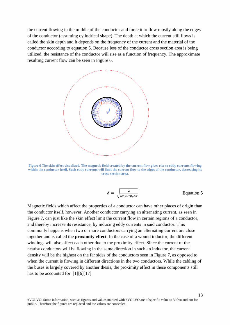
13 #VOLVO: Some information, such as figures and values marked with #VOLVO are of specific value to Volvo and not for
public. Therefore the figures are replaced and the values are concealed.
the current flowing in the middle of the conductor and force it to flow mostly along the edges
of the conductor (assuming cylindrical shape). The depth at which the current still flows is
called the skin depth and it depends on the frequency of the current and the material of the
conductor according to equation 5. Because less of the conductor cross section area is being
utilized, the resistance of the conductor will rise as a function of frequency. The approximate
resulting current flow can be seen in Figure 6.
Figure 6 The skin effect visualized. The magnetic field created by the current flow gives rise to eddy currents flowing
within the conductor itself. Such eddy currents will limit the current flow to the edges of the conductor, decreasing its
cross-section area.
𝛿 = √2
𝜔∗𝜇𝑟∗𝜇0∗𝜎 Equation 5
Magnetic fields which affect the properties of a conductor can have other places of origin than
the conductor itself, however. Another conductor carrying an alternating current, as seen in
Figure 7, can just like the skin effect limit the current flow in certain regions of a conductor,
and thereby increase its resistance, by inducing eddy currents in said conductor. This
commonly happens when two or more conductors carrying an alternating current are close
together and is called the proximity effect. In the case of a wound inductor, the different
windings will also affect each other due to the proximity effect. Since the current of the
nearby conductors will be flowing in the same direction in such an inductor, the current
density will be the highest on the far sides of the conductors seen in Figure 7, as opposed to
when the current is flowing in different directions in the two conductors. While the cabling of
the buses is largely covered by another thesis, the proximity effect in these components still
has to be accounted for. [1][6][17]

14 #VOLVO: Some information, such as figures and values marked with #VOLVO are of specific value to Volvo and not for
public. Therefore the figures are replaced and the values are concealed.
Figure 7 The proximity effect visualized. The field generated by the first conductor gives rise to eddy currents in the
second conductor, limiting its current flow. In the example given, the current is traveling in the same direction in both
conductors.
As current flows through an inductor consisting of windings wound around a core made of a
ferromagnetic material, there is also the effect of core saturation to consider. A core gets
saturated as the magnetic domains of the material it consists of all align themselves with an
applied external field. Depending on its application, this effectively sets a lower limit to the
size of a ferromagnetic core, as saturation can be avoided by having a large enough core and
therefore a large amount of magnetic domains to magnetize. From a circuit perspective, an
inductor with a saturated core will have its inductance affected by the current and alternating
currents flowing through a saturated core could be a cause of harmonics in the system. As
seen in Figure 8, the inductance typically drops rather drastically at the point of saturation.
The saturation effect is also noticeable for lower current levels with an increase in
temperature, as this causes the magnetic domains to align with an external field more easily.
For these reasons, inductors with ferromagnetic cores which are to be used in a TVS must be
dimensioned with the current ripple levels in mind (if only there was some way to predict
these beforehand).[5][14]
15 #VOLVO: Some information, such as figures and values marked with #VOLVO are of specific value to Volvo and not for
public. Therefore the figures are replaced and the values are concealed.
Figure 8 Inductance as a result of saturation in a typical ferrite core.
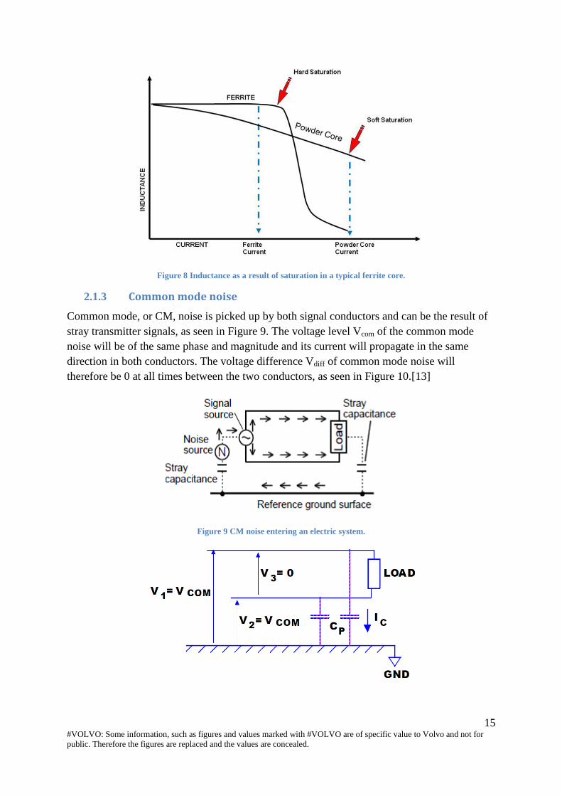
Common mode noise 2.1.3
Common mode, or CM, noise is picked up by both signal conductors and can be the result of
stray transmitter signals, as seen in Figure 9. The voltage level Vcom of the common mode
noise will be of the same phase and magnitude and its current will propagate in the same
direction in both conductors. The voltage difference Vdiff of common mode noise will
therefore be 0 at all times between the two conductors, as seen in Figure 10.[13]
Figure 9 CM noise entering an electric system.

16 #VOLVO: Some information, such as figures and values marked with #VOLVO are of specific value to Volvo and not for
public. Therefore the figures are replaced and the values are concealed.
Figure 10 Common mode noise difference between the two conductors. [13]
Differential mode noise 2.1.4
Noise that gives rise to currents flowing in opposite directions in the two conductors is known
as differential mode noise, henceforth referred to as DM noise or DM currents. DM noise
enters the system in the same way as the signal from a signal source, as seen in Figure 11.[13]
Figure 11 DM noise entering an electrical system.
The CM choke 2.1.5
In order to cancel CM signals, a common mode choke can be used. A choke can be made by
winding the two conductors around a common ferrite core as in Figure 12Figure 12. If the
conductors are wound in the opposite directions as seen from the same side, i.e. clockwise and
anti-clockwise, the choke is a CM choke. As the current passes through one of the conductors,
a magnetic field is generated inside the core. If two fields are generated in the same core at the
same time, the fields interact with each other. Two opposite fields counteract as the meet,
while two fields generated in the same direction add together. For common mode noise, the
result is the latter in a CM choke. The CM noise currents each generate a magnetic field in the
core which will be circulating in the same direction. This causes the currents to see a high
inductance as they enter the choke, which will ideally result in both noise currents canceling.
Currents flowing in different directions through the common mode filter, i.e. DM signals will
instead cause the magnetic fields of the core to be facing in opposite directions, as seen in
Figure 12. If the windings around the core are equal in number of windings the fields will
then cancel each other out instead. This theoretically results in a very low or zero inductance
for currents passing through the windings.

17 #VOLVO: Some information, such as figures and values marked with #VOLVO are of specific value to Volvo and not for
public. Therefore the figures are replaced and the values are concealed.
Figure 12 The structure of the windings and the equivalent circuit of a CM choke [13]
However, CM chokes are, like most electrical components, non-ideal. If the windings are not
perfectly balanced, for instance, the magnetic fields in the core will not cancel fully. This
results in a stray inductance, which typically corresponds to between 2-10 % of the CM
inductance. The windings also carry with them a small series resistance as well as a parallel
resistance and capacitance. In any electric vehicle, knowing these properties is essential in
order to accurately simulate the current ripple of the TVS. [9][15]
Measurement methods 2.2
An LCR meter can be used for various component measurements and provides high accuracy
over a broad spectrum of frequencies. It can be set to perform frequency sweeps and store the
results automatically and the voltage level can be given a DC bias if needed. It cannot,
however, be used in conjunction with an external source providing a larger current flow
through the test object. For measuring current dependency over a broad frequency spectrum, a
rig consisting of a custom built amplifier generally has to be used instead. Although it does
not allow for frequency dependency to be measured, certain measurements can also be
performed using a simple current transformer connected through a voltage transformer
directly to the electric grid.
2.2.1 LCR-measuring
A typical LCR meter is an instrument used for measuring impedance and its components. The
aforementioned impedance vector of an electrical component can be determined by measuring
the RMS values of the AC flowing through it, the voltage across its terminals, and the phase
difference between them. An LCR meter applying the automatic balance bridge method, as
most LCR meters do, can be used to perform these measurements by connecting the target to
the terminals of the LCR meter as seen in Figure 13.[8]
Figure 13 The automatic bridge method circuit design. Hc applies a measurement signal of wanted frequency, which
Lc receives and converts into a voltage based on the detected resistance. Hp and Lp marks the high and low potentials
of the measurement target.
When performing exact measurements on components with low impedance, residual
components in the test fixture come into play. These are unwanted parasitic characteristics
which affect the measured values. It can therefore be good practice to correct the measured
values by finding these residual components and adjust the measured values accordingly. This
is known as open correction and short correction, both of which most LCR meters are
designed to handle. In Figure 14, the equivalent circuit for the residual components of a
measurement target is shown. [8]

18 #VOLVO: Some information, such as figures and values marked with #VOLVO are of specific value to Volvo and not for
public. Therefore the figures are replaced and the values are concealed.
Figure 14 Equivalent circuit for the residual components of the test fixture.
Where Zm is the measured value, Zs is the short residual impedance, Y0 is the residual
admittance and Zx is the true value.
Equation 6 describes the relationship of the measured and residual values.
𝑍𝑚 = 𝑍𝑠 + 1
𝑌0+1
𝑍𝑥
Equation 6
Practically, an LCR meter can be used to perform measurements on a variety of components
such as capacitors, inductors and coils, transformers, piezoelectric elements, and contactless
IC cards. The signal frequency can typically be swept ranging from DC to a few hundred kHz
and the measured values can be stored on an external drive. However, LCR meters can rarely
handle external sources connected to the same sample and as the LCR meter usually does not
give off currents higher than a few hundred milliampere, finding the current dependency of
the measured component parameters is not possible.
2.2.2 Current transformer
Using a voltage transformer paired with a current transformer, some simple impedance
measurements can be performed using an oscilloscope or a multimeter. With the voltage
transformer connected to the electric grid and the current transformer connected between the
voltage transformer and the specimen, the current flowing through the specimen can be
increased significantly. The impedance can then be found using equation 1. In order to
determine the ratio of, for instance, resistance and inductance of the measured impedance, it is
required to perform some additional measurements as well. Either the phase shift in Figure 2
can be measured directly using an oscilloscope, or the purely resistive part in equation 4 can
be found by connecting the specimen to a power box feeding only DC, since ω then becomes
zero.

19 #VOLVO: Some information, such as figures and values marked with #VOLVO are of specific value to Volvo and not for
public. Therefore the figures are replaced and the values are concealed.
Figure 15 Current transformer setup
This method can be useful when determining the current dependency of the specimen
parameters. However, the frequency of the current will be set to the frequency of the grid
when using this method. In other words, it is not possible to find the current dependency in
conjunction with the frequency dependency of the component parameters.
2.2.3 Power Amplifier measurements
The custom built power amplifier measurement setup shown in Figure 16 was originally
designed to measure the properties of wound transformers and inductors with saturated cores,
but it can also be used to find both the current and frequency dependency of a load. This, by
default, takes all of the issues mentioned in chapter 2.1 into account. Using a computer as
controller, a waveform generator can be set to output specific current amplitudes at specific
frequencies. As the output levels are set by the waveform generator, a synchronization pulse
is sent to a trigg detector, which in turn tells the computer to start the data acquisition. This
signal can then be amplified by a power amplifier to generate higher current levels. The
current supplied to the load is measured with a precision shunt resistor via a voltage
difference amplifier. The load voltage can be measured by first scaling the direct voltage
down to levels between ±10 Volt using a LEM LV 25-P. The voltage and current signals can
then be acquired by the NI-9223 and stored in the computer. When calculating the impedance
based on the current and voltage levels acquired, the scaling factors of the shunt resistor and
the LEM have to be taken into consideration.

20 #VOLVO: Some information, such as figures and values marked with #VOLVO are of specific value to Volvo and not for
public. Therefore the figures are replaced and the values are concealed.
Figure 16 The power amplifier measurement setup
Equipment referenced in Figure 16:
1. Rigol DG1022
2. AE Techron 7796
3. National Instrument USB-6008
4. Ohmite TGHGC0500FE
5. INA117
6. LEM LV 25-P
7. National Instrument NI-9223 @ 1 MS/s
2.2.4 Battery measurements using a current injection transformer
A budget solution to performing measurements on batteries operating at higher voltages is by
injecting sinusoidal currents to the battery using a current injection transformer and measuring
the voltage and current at the battery terminals. The results of such measurements have been
verified using standard Electrochemical Impedance Spectroscopy (EIS) devices by Chalmers
University of Technology. For further explanations and measurement setup, see their report.
[18]

21 #VOLVO: Some information, such as figures and values marked with #VOLVO are of specific value to Volvo and not for
public. Therefore the figures are replaced and the values are concealed.
3. Traction Voltage System
Types of Traction Voltage Systems 3.1
The Traction Voltage System, TVS, consists of several different subsystems coupled together
with cables. All of Volvos bus model are equipped with versions of these utility providing
subsystems. What varies between the different bus models, however, is often only the
placement of the components and the quantity of components. A further introduction of the
different subsystems can be found in Subsystem specification.
3.1.1 Electric hybrid
Figure 17 shows a simplified block diagram of the 600V DC-system for Volvos electric
hybrid bus.
Figure 17 The DC-system for the electric hybrid bus.
3.1.2 Electric
Figure 18 shows a simplified block diagram of the 600V DC-system for Volvos electric bus.
As may be expected, the amount of batteries in the electric model is increased in order to
allow for the bus to travel longer distances on a single charge. Volvos electric bus platform in
figure 2 is currently in use on bus line 55 in Gothenburg, Sweden.

22 #VOLVO: Some information, such as figures and values marked with #VOLVO are of specific value to Volvo and not for
public. Therefore the figures are replaced and the values are concealed.
Figure 18 The DC-system for the electric bus.
3.1.3 TWIN MOTOR BUS1
The TWIN MOTOR BUS1 looks and behaves rather differently compared to its predecessors.
It is powered only by electricity and sports a carbon chassis so strong that no other structural
members are needed. This is not always for the best, however, as the thinner walls and lower
floor means less room for components and wiring. Conceptually, the idea is also for the
TWIN MOTOR BUS1 to be able to disassemble and assemble in a different fashion, such as
adding one or several joints and floor passenger area segments. Because of its unique
structure, the driving wheels of the bus have to be powered by different electric machines in
order for the bus to make the tight corners. From a current ripple perspective, this can
potentially result in new situations depending on how the electric motor drives are controlled.
A block diagram of the electrical system for the basic structure of the TWIN MOTOR BUS1
can be seen in Figure 19.

23 #VOLVO: Some information, such as figures and values marked with #VOLVO are of specific value to Volvo and not for
public. Therefore the figures are replaced and the values are concealed.
Figure 19 The DC-system for the TWIN MOTOR BUS1 #VOLVO
3.1.4 TWIN MOTOR BUS2
The TWIN MOTOR BUS2 is also powered completely by electricity. Figure 20 shows a
simplified block diagram of the 600V DC-system for Volvos Twin Motor bus2.
Figure 20 The DC-system for the Twin Motor bus2 #VOLVO

24 #VOLVO: Some information, such as figures and values marked with #VOLVO are of specific value to Volvo and not for
public. Therefore the figures are replaced and the values are concealed.
Subsystem specification 3.2
A number of basic requirements are found in all of Volvos buses. An engine or a motor
driving the vehicle forward and an energy storage system will cover the most fundamental
functions. In the case of the electric or electric hybrid model driving in electric mode, the
energy storage system consists of a battery. However, the ride would be a rather unpleasant
one without the other functions of the TVS. Lights, the control panel and the steering servo
are examples of functions powered by a low voltage system operating at 24 V. Connecting
this low voltage system to the 600 V system is a DCDC converter. Climate control and
ventilation is managed by the HVAC and an air compressor fills up tanks of pressurized air,
which can be used to operate the doors and kneel the bus. As there is no combustion engine to
provide heat to the passenger section in the winter, an electric heater is sometimes used in
fully electric vehicles as well. Lastly, an onboard charger is used to connect the TVS to a
charging station during a low power charge. The different subsystems are connected together
by cables in junction boxes as seen previously in the chapter. With the exception of the
junction boxes, all of these subsystems are equipped with filter components which affect the
properties of the TVS and the spreading of current ripple. Building on the previous project,
the load subsystems are equipped with current sources which represent their respective PECs.
3.2.1 MDS- Motor Drive System
Perhaps the biggest difference between a conventional vehicle and an electric is the
propulsion system. Electric machines as traction motors can be used for both propulsion and
braking, and provides high torque even at low speeds. Because the machine can work both as
a motor and a generator, the energy storage system can be replenished when applying the
brakes. The electric machines in both the electric and the electric hybrid are permanently
magnetized synchronous machines. The PEC’s in their respective models are equipped with
different filter components. Motor specifications can be seen in Table 2 and Table 3. For 600
V, the base speed presented is based on the maximum power of #VOLVO kW in the case of
the electric hybrid bus and #VOLVO kW in the case of the electric bus, according to the
supplier.
Table 2 Specification values for the EMD typ b
Converter type #VOLVO
Switching Frequency #VOLVO
Converter load type #VOLVO
Converter load power #VOLVO
Electric Machine base speed #VOLVO
Table 3 Specification values for the EMD typ c
Converter type #VOLVO
Switching Frequency #VOLVO
Converter load type #VOLVO

25 #VOLVO: Some information, such as figures and values marked with #VOLVO are of specific value to Volvo and not for
public. Therefore the figures are replaced and the values are concealed.
Converter load power #VOLVO
Electric Machine base speed #VOLVO
3.2.2 DCDC – Direct Current Converter
The DCDC converter is used to supply the low voltage side loads with power. Lights, panels,
steering servo, etc. make up a total maximum load of #VOLVO kW, as seen in Table 4. The
lowest voltage applied to reach full power can be used to calculate the converters duty cycle.
Table 4 Specification values for the DCDC
Converter type #VOLVO
Switching Frequency #VOLVO
Converter load type #VOLVO
Converter load power #VOLVO
Lowest voltage applied for full performance #VOLVO
3.2.3 Air compressor
The air compressed by the air compressor is used to kneel the bus, brake, and operate the
doors is also driven by an electric machine. The specifications for the PMSM used in this
application can be seen in Table 5. The lowest voltage applied to reach full power can be used
to calculate the converters duty cycle.
Table 5 Specification values for the Air Compressor
Converter type #VOLVO
Switching Frequency #VOLVO
Converter load type #VOLVO
Converter load power #VOLVO
Electric Machine base speed #VOLVO
Lowest voltage applied to reach base speed #VOLVO
3.2.4 HVAC - Heat Ventilation and Air Conditioning
The HVAC system is used to control the climate of the bus with regards to temperature and
ventilation. It is powered by an induction machine, which operates as shown in Table 6. The
lowest voltage applied to reach full power can be used to calculate the converters duty cycle.
Table 6 Specification values for the HVAC
Converter type #VOLVO
Switching Frequency #VOLVO
Converter load type #VOLVO
Converter load power #VOLVO

26 #VOLVO: Some information, such as figures and values marked with #VOLVO are of specific value to Volvo and not for
public. Therefore the figures are replaced and the values are concealed.
Electric Machine base speed #VOLVO
Lowest voltage applied to reach base speed
#VOLVO
3.2.5 Heater
Electric vehicles do not produce enough waste heat to keep the temperature of the passenger
area at a comfortable level during winter. For this purpose, an electric heater is installed in
Volvos fully electric vehicles. The heater operates at #VOLVO kW.
3.2.6 OnBC - On Board Charger
While the low power on board charger is only active while the vehicle is at standstill, its filter
components still affect and are affected by the current ripple when the loads are active.
Charging using the On Board Charger is not considered in this thesis.
3.2.7 Cable
Connecting the different components are the cables. The cables are dimensioned based on the
power of the component they are connected to. Volvo’s bus department uses 50 mm2 cables
for the batteries and the EMD, and 2x4 mm2 cables for the other loads. Cable measurements
are mainly performed as part of a separate thesis project.
3.2.8 ESS - Energy Storage System
In the existing bus models for Volvo’s electric and electric hybrid vehicles, a SAFT battery is
used as energy storage system. It has a nominal battery voltage of 633 Volt and a nominal
capacity of #VOLVO Ah and consists of 16 Li-ion modules in series, each containing 12
battery cells. Larger batteries typically exhibit a circuit behavior based on the characteristics
of the battery cells for lower frequencies and the battery rig for higher frequencies.
3.2.9 HJB – Hybrid Junction Box
The hybrid junction box serves as a merge point for cables and contains fuses. It contains no
other components and is not included in this thesis for evaluation.
3.2.10 CSU – Charging Switch Unit
The charging switch unit connects the TVS to the charging rails. Other than the cables
connected to it, it does not contain any impactful components and is not included in this thesis
for evaluation either.
27 #VOLVO: Some information, such as figures and values marked with #VOLVO are of specific value to Volvo and not for
public. Therefore the figures are replaced and the values are concealed.
4. Component measurements and impedance analysis As a first step of getting to know the system and identifying components of interest, a
sensitivity analysis was performed on the existing model.
As a certain frequency behavior was expected, LCR measurements were performed in order
to find the impedance as a function of frequency ranging from 100 Hz to 300 kHz. A curve
fitting script in MATLAB was used in order to find the equivalent series and parallel
parameters of the different components. The starting values provided to the script were found
by using the LCR meter’s function to measure equivalent parameter values.
Measurements using a current transformer operating at grid frequency were performed as an
early attempt at finding the current dependency of the common mode choke values. The
inductance and series resistance were found either by measuring the DC resistance and
calculating the inductance using Pythagoras’ theorem or by measuring the phase shift directly.
The Power Amplifier measurements were performed at the institute of industrial production at
LTH. Using their custom built rig seen in Figure 16, the impedance was measured as a
function of both frequency and current.
All measurements were performed on the DM properties of the components.
Sensitivity analysis 4.1
As the preexisting model was somewhat uncertain with regards to both component values and
model design, a simple sensitivity analysis was performed on the existing simulation model in
order to provide insight into how component changes affected the ripple. Together with an
estimation of which components were most likely to differ from their given values and which
components were available, the focus of the measurements was determined. The components
to measure based on the sensitivity analysis and availability are presented in Table 7.
Table 7 Result from the sensitivity analysis
Subsystem Component(s) to measure
EMD type b CM choke (DM properties)
DC-link capacitor
EMD type c CM choke (DM properties)
DC-link capacitor
DCDC CM choke (DM properties)
Air compressor CM choke (DM properties)
HVAC CM choke (DM properties)
OnBC CM choke (DM properties)
Battery Entire rig
Cables Entire cable (separate thesis project)

28 #VOLVO: Some information, such as figures and values marked with #VOLVO are of specific value to Volvo and not for
public. Therefore the figures are replaced and the values are concealed.
LCR measurements 4.2
Using the LCR meter, both the impedance and its reactive and resistive components were
measured as a function of frequency. Entering these values into the curve fitting script as
starting values provided equivalent component values which in turn yielded the total
impedance wanted for all frequencies. Schematics for all of the components see chapter 0.
4.2.1 EMD type B
In the hybrid bus EMD, measurements were performed on the CM choke and the DC-link
capacitors. The measured impedance as a function of frequency of the EMD type b capacitor
is shown in Figure 22 along with the fitted lines based on the impedance of the capacitor
model seen in Figure 3. Figure 25 shows the measured impedance as a function of frequency
of the CM choke as well as the fitted curves based on the impedance of the circuit seen in
Figure 4. The measured values from Figure 23 were used as reference to the curve fitting.
Table 9 shows the values of the equivalent series and parallel components for the CM choke.
The values for the equivalent components of the capacitor are shown in Table 8. The values
for the capacitor were measured by utilizing the DC-bias function of the LCR meter.
Table 8 Result of the curve fitting for the DC-link capacitance in EMD typ b
DC_link
Capacitance
C Rser Lser Rpar Cpar RLshunt
#VOLVO #VOLVO #VOLVO #VOLVO #VOLVO #VOLVO
Figure 21 (Figure 3 Equivalent circuit of a capacitor

29 #VOLVO: Some information, such as figures and values marked with #VOLVO are of specific value to Volvo and not for
public. Therefore the figures are replaced and the values are concealed.
Figure 22 Curve fitting of the DC-link capacitance in EMD type b

30 #VOLVO: Some information, such as figures and values marked with #VOLVO are of specific value to Volvo and not for
public. Therefore the figures are replaced and the values are concealed.
Figure 23 The Inductance and Resistance in the CM choke in EMD type b
Table 9 Result of the curve fitting for the CM-choke in EMD type b
CM-choke L Rser Cpar Rpar
#VOLVO #VOLVO #VOLVO #VOLVO

31 #VOLVO: Some information, such as figures and values marked with #VOLVO are of specific value to Volvo and not for
public. Therefore the figures are replaced and the values are concealed.
Figure 24 (Figure 4 Equivalent circuit of an inductor
Figure 25 Curve fitting of the CM-choke in EMD type b
4.2.2 EMD type C
For the EMD type c, measurements were performed to find the impedance as a function of
frequency of the CM choke and DC-link capacitor. The impedance of the CM choke is plotted
in Figure 27 along with the curve fitting impedance based on the equivalent circuit of an
inductor seen in Figure 4. The equivalent circuit parameters are shown in Table 11. The
measured DC-link capacitor impedance and its fitted curves are shown in Figure 26. Its
impedance is based on the equivalent circuit of a capacitor seen in Figure 3 with the values
presented in Table 10. The values for the capacitor were measured by utilizing the DC-bias
function of the LCR meter.

32 #VOLVO: Some information, such as figures and values marked with #VOLVO are of specific value to Volvo and not for
public. Therefore the figures are replaced and the values are concealed.
Table 10 Result of the curve fitting for the DC-link capacitance in EMD type c (equivalent circuit Figure 21)
DC_link
Capacitance
C Rser Lser Rpar Cpar RLshunt
#VOLVO #VOLVO #VOLVO #VOLVO #VOLVO #VOLVO
Figure 26 Curve fitting of the DC-link capacitance in EMD type c
Table 11 Result of the curve fitting for the CM-choke in EMD type c (equivalent circuit Figure 24)
CM-choke L Rser Cpar Rpar
#VOLVO #VOLVO #VOLVO #VOLVO

33 #VOLVO: Some information, such as figures and values marked with #VOLVO are of specific value to Volvo and not for
public. Therefore the figures are replaced and the values are concealed.
Figure 27 Curve fitting of the CM-choke in EMD typ c
4.2.3 DCDC
In the DCDC, only the CM choke was available without permanently destroying the circuit
board. Impedance measurement results are shown in Figure 29 along with the curve fitting
plots based on the equivalent circuit in Figure 4. The measured values in Figure 28 were used
as reference values to the curve fitting. The equivalent circuit component values are shown in
Table 12.

34 #VOLVO: Some information, such as figures and values marked with #VOLVO are of specific value to Volvo and not for
public. Therefore the figures are replaced and the values are concealed.
Figure 28 The Inductance and Resistance in the CM choke in DCDC
Table 12 Result of the curve fitting for the CM-choke in DCDC (equivalent circuit Figure 24)
CM-choke L Rser Cpar Rpar
#VOLVO #VOLVO #VOLVO #VOLVO

35 #VOLVO: Some information, such as figures and values marked with #VOLVO are of specific value to Volvo and not for
public. Therefore the figures are replaced and the values are concealed.
Figure 29 Curve fitting of the CM-choke in DCDC
4.2.4 Air compressor
Like in the DCDC, only the CM choke was available for measuring. Impedance measurement
results are shown in Figure 31 along with the curve fitting plots based on the equivalent
circuit in Figure 4. The measured values in Figure 30 were used as reference values to the
curve fitting. The equivalent circuit component values are shown in Table 13.

36 #VOLVO: Some information, such as figures and values marked with #VOLVO are of specific value to Volvo and not for
public. Therefore the figures are replaced and the values are concealed.
Figure 30 The Inductance and Resistance in the CM choke in Air Compressor
Table 13 Result of the curve fitting for the CM-choke in Air Compressor (equivalent circuit Figure 24)
CM-choke L Rser Cpar Rpar
#VOLVO #VOLVO #VOLVO #VOLVO

37 #VOLVO: Some information, such as figures and values marked with #VOLVO are of specific value to Volvo and not for
public. Therefore the figures are replaced and the values are concealed.
Figure 31 Curve fitting of the CM-choke in Air Compressor
4.2.5 HVAC
The CM choke was the only component available for measurement in the HVAC. Although
some measurements were performed on the entire board, a circuit representation was not
found as the initial values were impossible to measure without destroying the circuit. The
measured impedance of the CM choke is shown in Figure 33 along with the curve fitting plots
based on the equivalent circuit of an inductor seen in Figure 4. The measured values in Figure
32 were used as reference values to the curve fitting. The equivalent circuit component
values are shown in Table 14.

38 #VOLVO: Some information, such as figures and values marked with #VOLVO are of specific value to Volvo and not for
public. Therefore the figures are replaced and the values are concealed.
Figure 32 The Inductance and Resistance in the CM choke in HVAC
Table 14 Result of the curve fitting for the CM-choke in HVAC (equivalent circuit Figure 24)
CM L Rser Cpar Rpar
#VOLVO #VOLVO #VOLVO #VOLVO
39 #VOLVO: Some information, such as figures and values marked with #VOLVO are of specific value to Volvo and not for
public. Therefore the figures are replaced and the values are concealed.
Figure 33 Curve fitting of the CM-choke in HVAC
4.2.6 OnBC
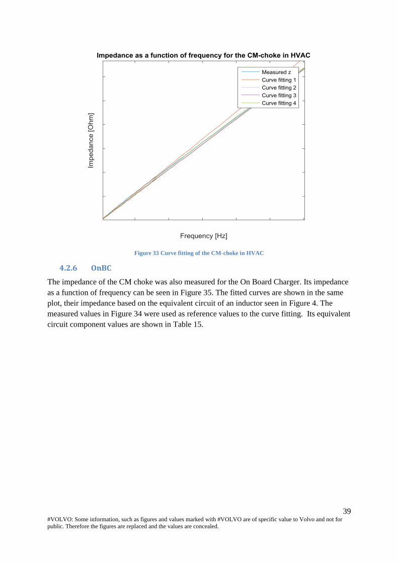
The impedance of the CM choke was also measured for the On Board Charger. Its impedance
as a function of frequency can be seen in Figure 35. The fitted curves are shown in the same
plot, their impedance based on the equivalent circuit of an inductor seen in Figure 4. The
measured values in Figure 34 were used as reference values to the curve fitting. Its equivalent
circuit component values are shown in Table 15.

40 #VOLVO: Some information, such as figures and values marked with #VOLVO are of specific value to Volvo and not for
public. Therefore the figures are replaced and the values are concealed.
Figure 34 The Inductance and Resistance in the CM choke in OnBC
Table 15 Result of the curve fitting for the CM-choke in OnBC (equivalent circuit Figure 24)
CM L Rser Cpar Rpar
#VOLVO #VOLVO #VOLVO #VOLVO

41 #VOLVO: Some information, such as figures and values marked with #VOLVO are of specific value to Volvo and not for
public. Therefore the figures are replaced and the values are concealed.
Figure 35 Curve fitting of the CM-choke in OnBC
4.2.7 Cables
Although some cable measurements were performed in order to provide placeholder values
for the cables during the course of the project, the cable values provided by the parallel thesis
project workers were eventually used in the model. The equivalent circuit model for the
cables was modeled based on the T model. The values were not based on a frequency
dependent model such as a curve fitting but instead selected based on the frequency of the
most powerful load.
Current transformer measurements at grid frequency 4.3
The measurement setup shown in Figure 15, was used in an attempt to measure the current
dependency of the impedance for all CM chokes. Vtop, Itop and the resistance in the setup was
measured and the impedance and inductance was calculated. The measurement results are
shown in Table 16.
Table 16 Current transformer measurement results. *=img
Z [Ω] L [H] R [Ω]
DCDC #VOLVO #VOLVO #VOLVO
Air Compressor #VOLVO #VOLVO #VOLVO
HVAC #VOLVO #VOLVO #VOLVO
OnBC #VOLVO #VOLVO* #VOLVO
42 #VOLVO: Some information, such as figures and values marked with #VOLVO are of specific value to Volvo and not for
public. Therefore the figures are replaced and the values are concealed.
Power Amplifier measurement 4.4
Measurements using the Power Amplifier measurement rig were performed on all CM
chokes. The available capacitors were excluded from the measurements, as the Power
Amplifier measurement rig was not built to output a DC-bias. The Impedance as a function of
both frequency and current for all components can be seen in Figure 36, Figure 37, Figure 38,
Figure 39, Figure 40 and Figure 41.
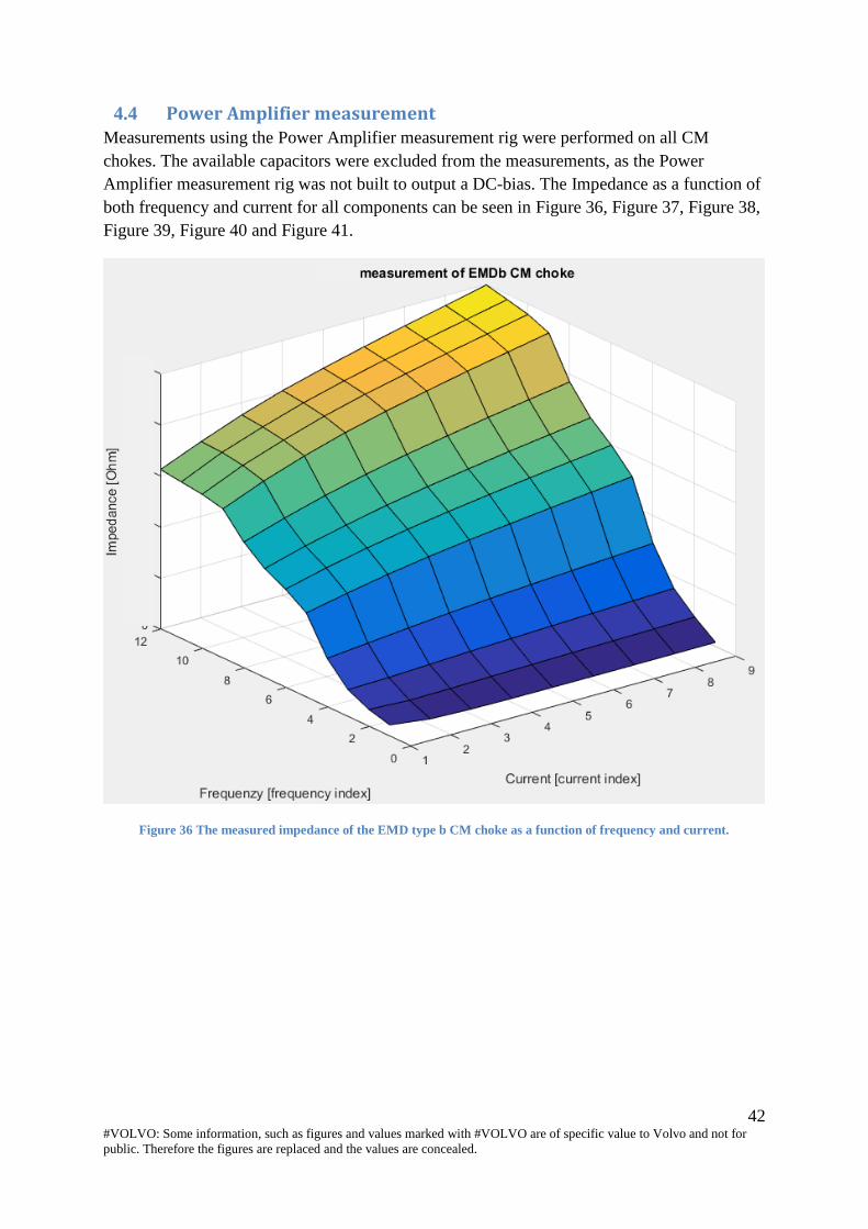
Figure 36 The measured impedance of the EMD type b CM choke as a function of frequency and current.
43 #VOLVO: Some information, such as figures and values marked with #VOLVO are of specific value to Volvo and not for
public. Therefore the figures are replaced and the values are concealed.
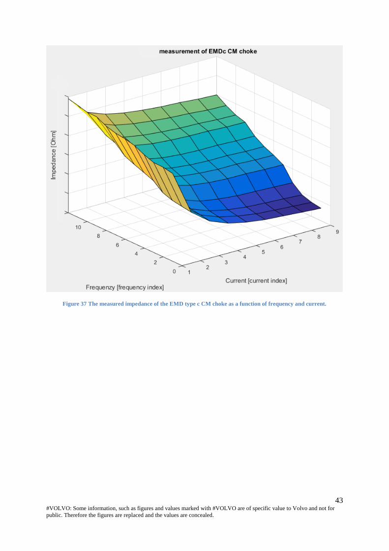
Figure 37 The measured impedance of the EMD type c CM choke as a function of frequency and current.

44 #VOLVO: Some information, such as figures and values marked with #VOLVO are of specific value to Volvo and not for
public. Therefore the figures are replaced and the values are concealed.
Figure 38 The measured impedance of the DCDC CM choke as a function of frequency and current.
45 #VOLVO: Some information, such as figures and values marked with #VOLVO are of specific value to Volvo and not for
public. Therefore the figures are replaced and the values are concealed.
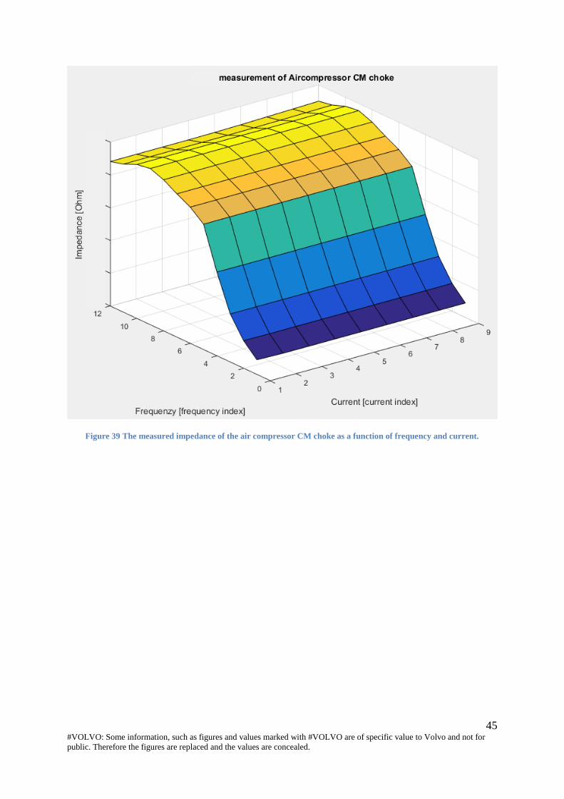
Figure 39 The measured impedance of the air compressor CM choke as a function of frequency and current.

46 #VOLVO: Some information, such as figures and values marked with #VOLVO are of specific value to Volvo and not for
public. Therefore the figures are replaced and the values are concealed.
Figure 40 The measured impedance of the HVAC CM choke as a function of frequency and current.

47 #VOLVO: Some information, such as figures and values marked with #VOLVO are of specific value to Volvo and not for
public. Therefore the figures are replaced and the values are concealed.
Figure 41 The measured impedance of the OnBC CM choke as a function of frequency and current.
As seen in chapter Power Amplifier measurement, the impedance of some of the major
components is affected both by frequency and current. The rise of impedance as a function of
frequency is likely due to the skin effect and the proximity effect, as they increase the
resistance by limiting the current flow. The current dependency seen in the Power Amplifier
measurements of the EMD type b, EMD type c, and on board charger, however, is slightly
harder to explain. Core saturation could be a guess in the case of the EMD type c and the on
board charger, as the impedance drops slightly with an increase in current. However, core
saturation is not very likely due to the fact that the chokes are CM chokes, which should be
able to handle DM signals such as the measurement signal of a higher magnitude without
saturating. As for the EMD type b, the impedance rises with an increased current. The
likeliest explanation to this is probably thermal dependency. During the measurement the
component became so warm that it was left to cool off before proceeding. In conjunction with
the increased resistance due to the higher frequency, the temperature will rise even higher and
faster, causing an enhanced rise in impedance. The effect of this can even be seen in some of
the other components, where the combination of a high frequency and a high current causes
the impedance to increase slightly. In a real vehicle, the components are mounted on a heat

48 #VOLVO: Some information, such as figures and values marked with #VOLVO are of specific value to Volvo and not for
public. Therefore the figures are replaced and the values are concealed.
sink meant to drain the heat. If the increased temperature during the measurements was the
source of the current dependency, perhaps the effect won’t be as prominent in a real vehicle.
The frequency behavior of the impedance seen in the Power Amplifier measurements does not
mirror the frequency behavior seen in the LCR measurements. This is likely due to the LEM
LV 25-P used to scale the voltage down later being found to do so as a function of frequency
for frequencies of about 3 kHz and higher. The current dependency for each frequency point
can still be seen, however, as all current points of the same frequency were attenuated by an
equal amount. While taking the frequency behavior into account in the model can be rather
easily done using a curve fitting script, doing the same for current dependency is hard. If the
current dependency is approximated to be constant independent of frequency, a rather crude
solution is to simply scale the measured impedance curve based on the current dependency
factor seen in the equation below.
𝐶𝑢𝑟𝑟𝑒𝑛𝑡 𝑑𝑒𝑝𝑒𝑛𝑑𝑒𝑛𝑐𝑦 𝑓𝑎𝑐𝑡𝑜𝑟 =𝐼𝑚𝑝𝑒𝑑𝑎𝑛𝑐𝑒 𝑎𝑡 𝑐𝑜𝑚𝑝𝑜𝑛𝑒𝑛𝑡 𝑟𝑖𝑝𝑝𝑙𝑒 𝑠𝑖𝑧𝑒
𝐼𝑚𝑝𝑒𝑑𝑎𝑛𝑐𝑒 𝑎𝑡 100 𝑚𝐴
Performing measurements meant to find the reactive and resistive part of the different
components by using a current transformer operating at grid frequency proved to be difficult.
The reactive part of the impedance was often so small due to the low frequency of the signal
that separating the impedance into its resistive and reactive components more often than not
yielded highly unlikely results. The current transformer setup could be used to provide an
estimation of the current dependency of the total impedance though, once again granted the
current dependency is approximated to be constant independent of frequency. The results can
then be used in conjunction with LCR measurements in order to provide an accurate model.
However, modeling a new bus will create a catch 22 as the current ripple size is unknown
until said bus has been constructed for real.
Another thing worth noting is that, while the LCR meter measurements are used as the
foundation for the resulting simulation model, the reactive measurements for lower
frequencies are probably not to be trusted for the same reason as explained above about the
current transformer measurements. The frequency of the measurement signal is simply too
low to provide a phase shift large enough to measure properly, as the somewhat loose
conditions wL >> R and wL >> 1/wC, or 1/wC >> R and 1/wC >> wL respectively no longer
hold. Also, no open and short correction of the values measured with the LCR meter was
performed. The reason for this being that moving the test fixture around even slightly was
estimated to introduce a larger error than what could be corrected for.

49 #VOLVO: Some information, such as figures and values marked with #VOLVO are of specific value to Volvo and not for
public. Therefore the figures are replaced and the values are concealed.
Battery measurements using a current injection transformer 4.5
Using a GAMRY measurement instrument, an attempt was made at measuring the impedance
of a 12 Volt car battery using the current injection transformer setup mentioned in chapter
Battery measurements using a current injection transformer. The measurements using the
GAMRY instrument were performed as a test before moving on to larger batteries, but as the
results proved unsatisfying, no further battery measurements were performed. The measured
impedance of a 2 Ohm resistor when the current transformer was connected between the
GAMRY instrument and the battery and when the GAMRY instrument was connected
directly to the battery is shown in Figure 42. With the help of the people at the Volvo
workshop, much of the battery measurement equipment was mounted on a wooden board and
isolated as a safety precaution. Hopefully this will make the process of performing
measurements on the batteries easier in the future.
Figure 42 The difference in measured impedance of a 2 Ohm resistor when the GAMRY was connected through the
current injection transformer (red) and when it was not (blue).
The brief battery measurements performed using the GAMRY did not yield very promising
results. As seen in the impedance measurements when testing the instrument, the results
differed depending on whether the current injection transformer was connected between the
GAMRY and the specimen or not. This effect is likely due this some filtering of the
measurements performed by the GAMRY itself, as its measurement probe and the injection
probe are originally meant to be in the same node. As the current injection transformer setup
is probably the simplest solution, an approach when using it with a different instrument
should be looked into.

50 #VOLVO: Some information, such as figures and values marked with #VOLVO are of specific value to Volvo and not for
public. Therefore the figures are replaced and the values are concealed.
Vehicle measurements performed by Volvo 4.6
Looking into the vehicle measurements performed by Volvo, several unexpected tendencies
were discovered. In order to give the simulation model a fighting chance in the verification,
these tendencies were also modeled to some extent. The following section presents some of
the results found, which to a large extent are based on measurements performed on the
electric hybrid bus with only one component active at a time. According to results provided
by the previous thesis project, the DC link current ripple produced by a PEC is at its worst
when the duty cycle is at 50 % [12]. The pulsed current loads of the simulation models are
therefore largely based on this case, if relevant.
4.6.1 EMD type b
Based on the vehicle measurements in the electric hybrid, the time when the EMD type b was
at 50 % duty cycle was found by looking at the FFT of the DC link current ripple. This time
was the matched to a mean current level, which in turn was used to model the worst case load
model of the EMD type b. As the speed of the motor increases, the amplitude of the total
current ripple seen in Figure 43 appears to increase as well. The frequencies which cause this
behavior appear to match the frequencies of the peaks seen in Figure 44. Looking at the
current ripple in Figure 45, the shape of the current ripple of the different frequencies can be
seen.
Figure 43 The total DC link current measured at the DC terminals of the EMD type b during acceleration at full
torque in the electric hybrid. Only the EMD is active. The changes in switching frequency can be seen as steps in the
current. The point at which the duty cycle reaches 50 % is marked by the vertical line.

51 #VOLVO: Some information, such as figures and values marked with #VOLVO are of specific value to Volvo and not for
public. Therefore the figures are replaced and the values are concealed.
Figure 44 The low frequency DC link current measured at the DC terminals of the EMD as a function of frequency in
the EMD type b in the electric hybrid. Only the EMD is active.
Figure 45 The DC link current measured at the DC terminals of the EMD as a function of frequency and time in EMD
type b in the electric hybrid. Only the EMD is active.

52 #VOLVO: Some information, such as figures and values marked with #VOLVO are of specific value to Volvo and not for
public. Therefore the figures are replaced and the values are concealed.
4.6.2 EMD type c
The vehicle measurements of the electric bus provided a good estimation of the current level
at 50 % duty cycle as well. This was used to model the worst case load model of the EMD
type c. The current ripple amplitude measured in the EMD type c as a function of time and
frequency can be seen in Figure 46.
Figure 46 The DC link current measured at the DC terminals of the EMD as a function of frequency and time in EMD
type c in the electric bus. Several components are active.
4.6.3 Dual EMD type c
Installing two electric motors in the same vehicle, as in the TWIN MOTOR BUS1, resulted in
some previously unseen behavior. Theoretically, if the on-pulse of the PECs of the two EMDs
were to be on at the same time, the current ripple as seen from the rest of the vehicle would
increase. Depending on the duty cycle, the opposite should occur if the two motors were
completely out of phase. In the case of 50 % duty cycle, this would theoretically mean no
current ripple whatsoever, as the two pulses added together creates a constant DC level. For
the same reason, the case when the two motors both operate at 25 % duty cycle can
potentially take the appearance of 50 % duty cycle to the rest of the circuit if the two motors
are out of phase. The distance between the motors also potentially has an effect on the current
ripple, as the length of the cables determines the impedance.
The ripple measured in the two EMDs during acceleration differs between different
measurements. In one instance, the two motors are operating in phase at the start of the
acceleration. As the change in switching frequency occurs, one of the motors changes its
switching frequency from #VOLVO to #VOLVO kHz sooner than the other. This results in an

53 #VOLVO: Some information, such as figures and values marked with #VOLVO are of specific value to Volvo and not for
public. Therefore the figures are replaced and the values are concealed.
imbalance between the motors. As the second motor also changed its switching frequency, the
motors were once again operating in phase. However, during the time of the acceleration, the
current pulses would slowly drift apart, once again resulting in a slight imbalance between the
two. In other measurements, the pulsed currents of the two motors drift in and out of phase in
a different manner and the current ripple as a result is vastly different. In order to properly
verify a model simulating the current ripple of the DC link of the TWIN MOTOR BUS1, it is
therefore required looking at many different measurements and adjust the pulsed current loads
representing the motors of the model appropriately.
4.6.4 DCDC
The DCDC was found to be giving off a DC link current ripple fundamental frequency of
#VOLVO kHz rather than the previously thought #VOLVO kHz. The true shape of this ripple
was unclear due to the relatively low sampling frequency, but as the DCDC converter is not
used to power a motor, the estimation provided by the previous master thesis that the lowest
voltage applied for full performance in conjunction with the battery voltage and the rated
power can be used to calculate the duty cycle was used [12]. The mean current of the fully
loaded DCDC was used together with its duty cycle in order to model the load.
4.6.5 Air compressor
Investigating the curve form of the DC link current ripple generated by the air compressor in
the electric hybrid, it was found that the air compressor PEC likely operates at 52 % duty
cycle. The previously estimated duty cycle was 83 %. The mean current level was used in
conjunction with the duty cycle to approximate a model for the air compressor load. The
zoomed in current ripple of the air compressor can be seen in Figure 47.
Figure 47 DC link current ripple as a function of time measured on the DC terminals of the air compressor PEC in
the electric hybrid.

54 #VOLVO: Some information, such as figures and values marked with #VOLVO are of specific value to Volvo and not for
public. Therefore the figures are replaced and the values are concealed.
4.6.6 HVAC
The ripple in the HVAC is somewhat affected by the AC load. While this was previously
established, a further investigation of the ripple waveform, Figure 48, in the electric hybrid
shows that the PEC of the HVAC operates at a duty cycle of 51 %. The previously estimated
duty cycle was 93 %. The HVAC load was modeled using the mean current level during
operation and the duty cycle.
Figure 48 Current ripple as a function of time, in the HVAC in the electric hybrid.
4.6.7 Battery
The previous battery model was largely based on the impedance of a single battery cell, which
was then multiplied by the amount of cells in a battery pack. However, recent studies
performed by Chalmers indicate that the impedance of the cells is insignificant in comparison
to the impedance of the battery rig for higher frequencies (usually at about 1 kHz and more,
depending on the battery).

55 #VOLVO: Some information, such as figures and values marked with #VOLVO are of specific value to Volvo and not for
public. Therefore the figures are replaced and the values are concealed.
5. Simulation model structure The circuit models are largely based on the preexisting models, which in turn rely on data
from component owners at Volvo and their suppliers. The components for which
measurements are performed are updated according to their respective equivalent circuits
found in chapter 4.2Component measurements and impedance analysis. Some of the
simulation model pulsed current loads are also updated based on new measurements provided
by Volvo in order to more accurately represent the current and voltage levels. For the EMD in
the electric hybrid bus, a special source is modeled in order to simulate the entire acceleration.
This is only possible in the electric hybrid bus because no other load is active in the vehicle
measurements. All component values not mentioned are provided by Volvo during this or the
previous thesis project and remain unchanged.
Electric hybrid 5.1
Not much has changed in the electric hybrid model as the base structure is the same. The
simulation model can be seen in Figure 49.
Figure 49 The simulation model of the electric hybrid
Electric 5.2
The structural simulation model for the electric bus can be seen in Figure 50.

56 #VOLVO: Some information, such as figures and values marked with #VOLVO are of specific value to Volvo and not for
public. Therefore the figures are replaced and the values are concealed.
Figure 50 The simulation model of the electric bus
TWIN MOTOR BUS1 5.3
The model for the TWIN MOTOR BUS1 was made from scratch along with the TWIN
MOTOR BUS1 model library. A special model was also made in order to be able replicate the
behavior seen in the vehicle measurements in which the two motors drift apart and change
switching frequency independently. The different simulation models can be seen in Figure 51
and Figure 52.
Figure 51 The simulation model of the TWIN MOTOR BUS1 #VOLVO

57 #VOLVO: Some information, such as figures and values marked with #VOLVO are of specific value to Volvo and not for
public. Therefore the figures are replaced and the values are concealed.
Figure 52 The simulation model, of the TWIN MOTOR BUS1, used to simulate the effects of dual motors #VOLVO
TWIN MOTOR BUS2 5.4
The structural simulation model of the TWIN MOTOR BUS2 can be seen in in Figure 53.
The TWIN MOTOR BUS2 contains both the 70 mm2 cable and the 95mm
2 cable (which has
not been modeled yet). The Twin Motor bus2 model was made along with its model library.
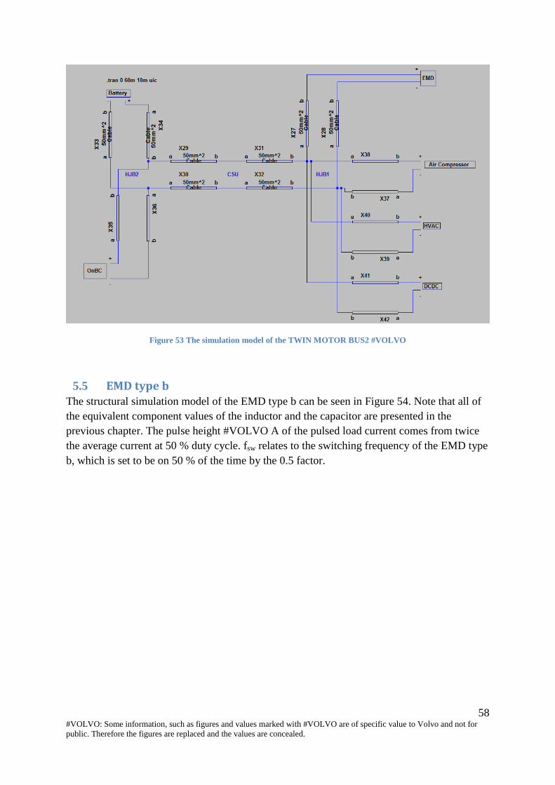
58 #VOLVO: Some information, such as figures and values marked with #VOLVO are of specific value to Volvo and not for
public. Therefore the figures are replaced and the values are concealed.
Figure 53 The simulation model of the TWIN MOTOR BUS2 #VOLVO
EMD type b 5.5
The structural simulation model of the EMD type b can be seen in Figure 54. Note that all of
the equivalent component values of the inductor and the capacitor are presented in the
previous chapter. The pulse height #VOLVO A of the pulsed load current comes from twice
the average current at 50 % duty cycle. fsw relates to the switching frequency of the EMD type
b, which is set to be on 50 % of the time by the 0.5 factor.

59 #VOLVO: Some information, such as figures and values marked with #VOLVO are of specific value to Volvo and not for
public. Therefore the figures are replaced and the values are concealed.
Figure 54 The simulation model of the EMD type b
EMD type c 5.6
Figure 55 shows the simulation model of the EMD type c used in the fully electric bus. All of
the values of the measured components can be found in the previous chapter. The pulse height
#VOLVO A of the pulsed load current comes from twice the average current at 50 % duty
cycle. #VOLVO relates to the switching frequency of the EMD type b at 11.2 % duty cycle as
an example of how to simulate the #VOLVO kHz current ripple in the DC link at the point
just before the change in switching frequency occurs. In order to simulate the current ripple
produced in the DC link by the EMD type c operating at 50 % duty cycle, the rightmost input
values can be changed to #VOLVO s and #VOLVO s, respectively.
Figure 55 The simulation model of the EMD typ c #VOLVO
(0, Pulse height, 0, 0, 00.5/ fsw1/ fsw )
(0, Pulse height, 0, 0, 00.112/ fsw1/ fsw
)

60 #VOLVO: Some information, such as figures and values marked with #VOLVO are of specific value to Volvo and not for
public. Therefore the figures are replaced and the values are concealed.
DCDC 5.7
In the DCDC model, Figure 56, the missing CM filter has been added in the model. The
equivalent components of the CM choke are presented in the previous chapter. The duty cycle
of the pulsed current load is 79.4 % according to the formula provided by the previous thesis
project. The amplitude of the pulse is calculated by dividing the mean current of the fully
loaded DCDC by #VOLVO.
Figure 56. The simulation model of the DCDC #VOLVO
Air compressor 5.8
The simulation model of the air compressor subsystem can be seen in Figure 57. The CM
choke is updated with the curve fitting parameters in the previous chapter. The pulsed current
load is updated based on the current behavior of the air compressor measured in the electric
hybrid bus, which in the previous chapter is estimated to be roughly 52 %. The height of the
current pulse is the result of dividing the mean current by the duty cycle.
(0, Pulse height, 0, 0, 00.794/ fsw1/ fsw
)

61 #VOLVO: Some information, such as figures and values marked with #VOLVO are of specific value to Volvo and not for
public. Therefore the figures are replaced and the values are concealed.
Figure 57 The simulation model of the Air Compressor #VOLVO
HVAC 5.9
The CM choke of the HVAC is updated based on the curve fitting parameters. All of the
parameters and the vehicle measurements which the pulsed current load is based on can be
seen in the previous chapter. The pulsed current load has been updated based on the current
behavior of the HVAC measured in the electric hybrid bus, which in the previous chapter is
estimated to be 51.2 %. The height of the current pulse is the result of dividing the mean
current by the duty cycle. The simulation model of the HVAC can be seen in Figure 58.
Figure 58 The simulation model of the HVAC #VOLVO
OnBC 5.10
As the on board charger is not active, no current or voltage source is included in the model, as
seen in Figure 59. The component is still affected by current ripple, however. All of its CM
choke parameters can be seen in the previous chapter.
(0, Pulse height, 0, 0, 00.52/ fsw1/ fsw )
(0, Pulse height, 0, 0, 00.512/ fsw1/ fsw
)

62 #VOLVO: Some information, such as figures and values marked with #VOLVO are of specific value to Volvo and not for
public. Therefore the figures are replaced and the values are concealed.
Figure 59 The simulation model of the OnBC #VOLVO
Battery 5.11
The battery model seen in Figure 60 remains relatively unchanged. The series resistance and
inductance are based on measurements performed on a single battery cell during the previous
thesis project. The voltage level can preferably be changed depending on the voltage level
wanted in the system. Other component values are based on specifications provided by Volvo
during the previous thesis project.
Figure 60 The simulation model of the battery
Cables 5.12
Cable measurements were performed as part of a separate thesis project in which it was also
investigated how the placement and connection points of the cables affect its behavior. The
existing simulation model was updated based on these values and modeled as a T for all cable
types. The cable values were based on the frequency deemed most prominent in the respective
TVS they were used in and not based on a curve fitted model.
(#VOLVO)

63 #VOLVO: Some information, such as figures and values marked with #VOLVO are of specific value to Volvo and not for
public. Therefore the figures are replaced and the values are concealed.
5.12.1 50 mm2
The model for the 50 mm2 cable can be seen in Figure 61. The values shown are in per
millimeter and hold true for frequencies of #VOLVO kHz.
Figure 61 The simulation model of the 50mm2 cable
5.12.2 4x2 mm2
The model for the 2x4 mm2 cable can be seen in Figure 62. The values shown are in per
millimeter and hold true for frequencies of #VOLVOkHz.
Figure 62 The simulation model of the 4x2mm2 cable
5.12.3 70 mm2
The model for the 70 mm2 cable can be seen in Figure 63. The values shown are in per
millimeter and hold true for frequencies of #VOLVO kHz.
Figure 63 The simulation model of the 70mm2 cable
Heater 5.13
The simulation model of the electric heater remains unchanged, as seen in Figure 64.

64 #VOLVO: Some information, such as figures and values marked with #VOLVO are of specific value to Volvo and not for
public. Therefore the figures are replaced and the values are concealed.
Figure 64 The simulation model of the Heater
Frequency analysis source 5.14
Utilizing the built-in AC analysis tool in LTSpice, a special pulsed current load can be made
in order to find the frequency behavior of the simulation model. This load can be seen in
Figure 65 along with the operational directive to sweep the frequency from 100 Hz to 100
kHz. To perform the simulation, the pulsed current loads presented earlier in the chapter are
exchanged for the AC source and the operational directive exchanged for the one presented in
the figure.
Figure 65 The current source and operational directive used in the AC analysis

65 #VOLVO: Some information, such as figures and values marked with #VOLVO are of specific value to Volvo and not for
public. Therefore the figures are replaced and the values are concealed.
6. Verification In the verification of the simulation model, many parameters are considered and adjusted for.
The battery voltage is set to match the voltage level of the battery in the vehicle at the time of
50 % duty cycle in the case of an accelerating EM. The cable values, received from the other
master thesis, are based on the measurements at the most prominent frequency, which is
usually the switching frequency of the EMD. Some of the pulsed current loads are, as
mentioned in the previous chapter, updated based on the vehicle ripple. To compare the
current ripple for different frequencies, an FFT using a flat top windowing function is used for
both the simulated and measured values. The AC analyses meant to find current frequencies
which can potentially be harmful to components in the DC link of the respective bus models
are presented. For the AC analyses, the pulsed current sources are exchanged for AC sources,
which are set to sweep the frequency from 100 Hz to 100 kHz.
Electric hybrid 6.1
The visualization of the ripple in the acceleration test can be seen in Figure 66 along with the
measured vehicle ripple. The verification for all components in the electric hybrid can be seen
in Table 17. A similar verification using a battery model in which the inductance is “tuned” to
be accurate when the EMD is active can be seen in Table 18. Note that the measurement
probe to the DCDC fell off during the vehicle test. The AC analysis of the electric hybrid is
presented in Figure 67.
Figure 66 The DC link current ripple measured on the DC terminals of the EMD of the electric hybrid (blue) and the
equivalent simulated current ripple (red) during an acceleration at full torque.

66 #VOLVO: Some information, such as figures and values marked with #VOLVO are of specific value to Volvo and not for
public. Therefore the figures are replaced and the values are concealed.
Table 17 Verification of the current ripple in the electric hybrid.
EMD active
@
#VOLVO
kHz
DCDC active
@ #VOLVO
kHz
HVAC active @
#VOLVO kHz
(Not FFT)
Air Com active
@ #VOLVOkHz
EMD Simulation #VOLVO #VOLVO #VOLVO #VOLVO
Vehicle #VOLVO #VOLVO #VOLVO #VOLVO
Difference +10.1 % -42.3 % +71.4 %
-13.9 % @ #VOLVO
kHz
-39.0 % @ #VOLVO
kHz
DCDC Simulation #VOLVO #VOLVO #VOLVO #VOLVO
Vehicle #VOLVO #VOLVO #VOLVO #VOLVO
Difference NaN NaN NaN NaN
HVAC Simulation #VOLVO #VOLVO #VOLVO #VOLVO
Vehicle #VOLVO #VOLVO #VOLVO #VOLVO
Difference -4.4 % -60 % +74.0 %
-35.0 % @ #VOLVO
kHz
-80.8 % @ #VOLVO
kHz
+32.0 % @ #VOLVO
kHz
Air Comp Simulation #VOLVO #VOLVO #VOLVO #VOLVO
Vehicle #VOLVO #VOLVO #VOLVO #VOLVO
Difference -35.3 % -33.3 % -50.2 % -15.0 %
OnBC Simulation #VOLVO #VOLVO #VOLVO #VOLVO
Vehicle #VOLVO #VOLVO #VOLVO #VOLVO
Difference +26.2 % -25 % -15.6 %
+630 % @ #VOLVO
kHz
-72.7 % @ #VOLVO
kHz
-76.9 % @ #VOLVO
kHz
ESS Simulation #VOLVO #VOLVO #VOLVO #VOLVO
Vehicle #VOLVO #VOLVO #VOLVO #VOLVO
Difference -89.5 % NaN -92.5 %
NaN @ #VOLVO kHz
-38.4 % @ #VOLVO
kHz
-97.2 % @ #VOLVO
kHz

67 #VOLVO: Some information, such as figures and values marked with #VOLVO are of specific value to Volvo and not for
public. Therefore the figures are replaced and the values are concealed.
Table 18 Verification of the electric hybrid. The battery inductance has been adjusted to #VOLVO H in order to yield
a matching current ripple in the battery when the EMD is running.
EMD active
@ #VOLVO
kHz
DCDC active
@ #VOLVO
kHz
HVAC active
@ #VOLVO
kHz
Air Comp active @
#VOLVO kHz
EMD Simulation #VOLVO #VOLVO #VOLVO #VOLVO
Vehicle #VOLVO #VOLVO #VOLVO #VOLVO
Difference -32.6 % -42.3 % +50.6 %
-12.2 % @ #VOLVO
kHz
-40 % @ #VOLVO kHz
DCDC Simulation #VOLVO #VOLVO #VOLVO #VOLVO
Vehicle #VOLVO #VOLVO #VOLVO #VOLVO
Difference NaN NaN NaN NaN
HVAC Simulation #VOLVO #VOLVO #VOLVO #VOLVO
Vehicle #VOLVO #VOLVO #VOLVO #VOLVO
Difference -13.3 % -60 % +70.5 %
-35 % @ #VOLVO kHz
-81.5 % @#VOLVO
kHz
+34 % @ #VOLVO
kHz
Air
Comp Simulation
#VOLVO #VOLVO #VOLVO #VOLVO
Vehicle #VOLVO #VOLVO #VOLVO #VOLVO
Difference -35.3 % -67 % -55.2 % -15.0 %
OnBC Simulation #VOLVO #VOLVO #VOLVO #VOLVO
Vehicle #VOLVO #VOLVO #VOLVO #VOLVO
Difference +26.2 % -65 % -38.7 %
+660 % @ #VOLVO
kHz
-74.5 % @#VOLVO
kHz
-80.2 % @ #VOLVO
kHz
ESS Simulation #VOLVO #VOLVO #VOLVO #VOLVO
Vehicle #VOLVO #VOLVO #VOLVO #VOLVO
Difference +0.1 % -92.0 % -29.3 %
NaN @#VOLVO kHz
+28 % @#VOLVO kHz
-94.3 % @#VOLVO
kHz

68 #VOLVO: Some information, such as figures and values marked with #VOLVO are of specific value to Volvo and not for
public. Therefore the figures are replaced and the values are concealed.
Figure 67 The AC analysis of the electric hybrid. The DC link current as a function of frequency measured at the
terminals of the different loads. In the bottom window: EMD type b (green), the air compressor (blue), and the HVAC
(red). In the upper window the DCDC (cyan), the OnBC (magenta), and the battery (gray).
Electric The verification of the electric bus can be seen in Table 19. The AC analysis results can be
seen in Figure 68.

69 #VOLVO: Some information, such as figures and values marked with #VOLVO are of specific value to Volvo and not for
public. Therefore the figures are replaced and the values are concealed.
Table 19 Verification of the electric bus
EMD active @
#VOLVO &
#VOLVO kHz
DCDC active
@ #VOLVO
kHz
HVAC active
(No file
found)
Air Com active
@ #VOLVO kHz
EMD Simulation #VOLVO #VOLVO #VOLVO #VOLVO
Vehicle #VOLVO #VOLVO #VOLVO #VOLVO
Difference
-96% @ #VOLVO
kHz
-46.5% @ #VOLVO
kHz -38%
-1%
DCDC Simulation #VOLVO #VOLVO #VOLVO #VOLVO
Vehicle #VOLVO #VOLVO #VOLVO #VOLVO
Difference
5% @ #VOLVO
kHz
22% @ #VOLVO
kHz -72.6%
30% @ #VOLVO kHz
-84% @ #VOLVO
kHz
NaN @ #VOLVO kHz
HVAC Simulation #VOLVO #VOLVO #VOLVO #VOLVO
Vehicle #VOLVO #VOLVO #VOLVO #VOLVO
Difference
NaN @ #VOLVO
kHz
10% @ #VOLVO
kHz NaN
NaN
Air
Comp Simulation
#VOLVO #VOLVO #VOLVO #VOLVO
Vehicle #VOLVO #VOLVO #VOLVO #VOLVO
Difference
41.7% @ #VOLVO
kHz
1% @ #VOLVO
kHz NaN
-3.2%
OnBC Simulation #VOLVO #VOLVO #VOLVO #VOLVO
Vehicle #VOLVO #VOLVO #VOLVO #VOLVO
Difference
20% @ #VOLVO
kHz -84%
NaN
ESS1 Simulation #VOLVO #VOLVO #VOLVO #VOLVO
Vehicle #VOLVO #VOLVO #VOLVO #VOLVO
Difference - -
ESS2 Simulation #VOLVO #VOLVO #VOLVO #VOLVO
Vehicle #VOLVO #VOLVO #VOLVO #VOLVO
Difference
ESS3 Simulation #VOLVO #VOLVO #VOLVO #VOLVO
Vehicle #VOLVO #VOLVO #VOLVO #VOLVO
Difference
ESS4 Simulation #VOLVO #VOLVO #VOLVO #VOLVO
Vehicle #VOLVO #VOLVO #VOLVO #VOLVO
Difference

70 #VOLVO: Some information, such as figures and values marked with #VOLVO are of specific value to Volvo and not for
public. Therefore the figures are replaced and the values are concealed.
The peak at #VOLVO kHz corresponds to the ripple before the change in switching frequency
(0.1117 % duty cycle). The few decimals are due to dewesoft not providing more.
Figure 68 The AC analysis of the electric bus. The DC link current as a function of frequency measured at the
terminals of the different loads. In the bottom window: EMD type c (green), air compressor (blue), HVAC (red). In
the top window: DCDC (cyan), OnBC (magenta), Batteries 1-4 (gray, dark green, dark blue, brown).
TWIN MOTOR BUS1 6.2
The verification of the TWIN MOTOR BUS1 when the EMD-loads are in perfect sync can be
seen in Table 20Table 20 Verification of the TWIN MOTOR BUS1. The results of the AC
analysis can be seen in Figure 69. The AC analysis of the TWIN MOTOR BUS1 with the
DCDCs removed can be seen in Figure 70 and Figure 71.
Table 20 Verification of the TWIN MOTOR BUS1
Motors in
sync
EMD:s active @
#VOLVO kHz
DCDC:s active
@ #VOLVO
kHz
Air Comp active
@ #VOLVO kHz
EMD left Simulation #VOLVO #VOLVO #VOLVO #VOLVO
EMD right Simulation #VOLVO #VOLVO #VOLVO #VOLVO
DCDC roof Simulation #VOLVO #VOLVO #VOLVO #VOLVO
DCDC
motor room Simulation
#VOLVO #VOLVO #VOLVO #VOLVO
Air comp. Simulation #VOLVO #VOLVO #VOLVO #VOLVO
OnBC Simulation #VOLVO #VOLVO #VOLVO #VOLVO
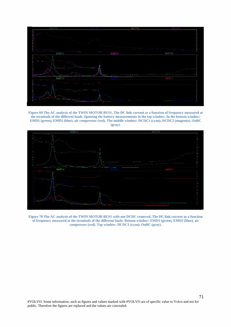
71 #VOLVO: Some information, such as figures and values marked with #VOLVO are of specific value to Volvo and not for
public. Therefore the figures are replaced and the values are concealed.
Figure 69 The AC analysis of the TWIN MOTOR BUS1. The DC link current as a function of frequency measured at
the terminals of the different loads. Ignoring the battery measurements in the top window. In the bottom window:
EMD1 (green), EMD2 (blue), air compressor (red). The middle window: DCDC1 (cyan), DCDC2 (magenta), OnBC
(gray).
Figure 70 The AC analysis of the TWIN MOTOR BUS1 with one DCDC removed. The DC link current as a function
of frequency measured at the terminals of the different loads. Bottom window: EMD1 (green), EMD2 (blue), air
compressor (red). Top window: DCDC1 (cyan), OnBC (gray).

72 #VOLVO: Some information, such as figures and values marked with #VOLVO are of specific value to Volvo and not for
public. Therefore the figures are replaced and the values are concealed.
Figure 71 The AC analysis of the TWIN MOTOR BUS1 bus with one DCDC removed. The DC link current as a
function of frequency measured at the terminals of the different loads. Bottom window: EMD1 (green), EMD2 (blue),
air compressor (red). Top window: DCDC2 (cyan), OnBC (gray).
TWIN MOTOR BUS2 6.3
There are no measurements to compare the TWIN MOTOR BUS2 model to. The AC analysis
of the model results in the behavior seen in Figure 72.
Figure 72 The AC analysis of the TWIN MOTOR BUS2 model. The DC link current as a function of frequency
measured at the terminals of the different loads. Ignoring the battery and HVAC measurements in the top window.
Bottom window: EMD1 (green), EMD2 (blue), air compressor (red). Middle window: DCDC1 (cyan), DCDC2
(magenta), OnBC (gray).
The acceleration test, in which the current load source of the electric hybrid bus was set to
mimic the switching frequency and duty cycle of a real acceleration, is to be taken with a
grain of salt. While it appears in Figure 43 as if the simulated current ripple deviates by a
large amount for higher speeds, the truth of the matter is revealed when zooming in on the
ripple measured in the bus. The real ripple at #VOLVO kHz rather well mimics the shape

73 #VOLVO: Some information, such as figures and values marked with #VOLVO are of specific value to Volvo and not for
public. Therefore the figures are replaced and the values are concealed.
vaguely appearing in the simulation. However, there are other, lower frequencies, which also
come into play at higher speeds. These can be seen in the zoomed in 3D plot of the EMD
current plotted against time and frequency in Figure 44 as increasing in frequency. The
frequencies of the peaks are likely tied to the speed of the electric motor.
The simulated current ripple values did, as can be seen in Table 17,Table 19 and Table 20, not
fall within the 10 % margin of the measured values when the models were based solely on the
measured values. The pulsed current loads did not always result in the same behavior as seen
in the vehicle measurements with regards to mean current and ripple amplitude either. As
some of the components have not been measured at all, namely the battery, this is not very
surprising. While probably accurate for the measured frequencies, the frequency dependency
of the cables has not been modeled either. As made clear by the verification of the
experimental battery inductance tests, tuning the models by simply changing the inductance of
the components is likely not possible. Instead, measurements which result in a curve fitted
impedance based on a more complex model are required. Until then, tuning of the load
models and further in depth verification of the current ripple is wasted.
Verification of the AC analysis model was made by comparing it to one single known value:
#VOLVO kHz. The previous EMD switching frequency of #VOLVO kHz had to be removed
because its ripple (at #VOLVO kHz) would destroy the DCDC. The AC analysis does offer
some insight as to why that is, as the current peaks of either one of the two types of EMD and
the DCDC reach a peak around #VOLVO kHz. A similar behavior can be seen at around
#VOLVO kHz involving the EMD type c, the DCDC, the on board charger, and to some
extent the air compressor. The AC analysis model is likely more accurate than the transient
model, in part due to the fact that mainly qualitative analysis of which frequencies are
dangerous is needed. The sensitive frequencies also seem to be affected mostly by the
components affected in turn by the resonance. In other words, if resonance of some sort
occurs between the EMD and the DCDC, as seen in the electric hybrid, the influence of, for
instance, the battery is diminished. This hypothesis is somewhat confirmed by removing
components. Unless a removed component is involved in the resonance, the resonance
remains at about the same frequency and amplitude. What seems to influence the resonance,
however, is the distance between the components, as seen when the different DCDCs are
removed in the TWIN MOTOR BUS1. Worth noting is also that a source not involved in the
resonance itself can still cause resonance elsewhere in the system, although the effect will be
slightly attenuated. Practically this means that no component which creates ripple at
#VOLVO kHz or #VOLVO kHz can be used in the same system as the components in use
today. To sum up, the AC analysis can probably be made even more accurate by adjusting the
cable measurements based on some sort of curve fitting, as the resonance seems to be affected
by the distance between the resonating components (and therefore the cable parameters). The
unfinished battery model, however, does not seem to influence the AC analysis noticeably
either when altered slightly or removed completely. For this reason, the AC analysis model is
likely to be more useful as of right now than the transient analysis model.

74 #VOLVO: Some information, such as figures and values marked with #VOLVO are of specific value to Volvo and not for
public. Therefore the figures are replaced and the values are concealed.
7. Conclusion
Results conclusion 7.1
Although the verification of the model in general does not point to any major advancement
with regards to model accuracy, the project still brought with it some useful results.
Using an LCR meter together with a curve fitting script yields promising results and can be
done easily when acquiring new components in the future. Looking into the current
dependency of the components, some components clearly appear more susceptible than
others. Modeling for this dependency is hard using LTSpice, and the true effects of current
dependency in a real vehicle may not be accurately represented by a model based on single
component measurements.
As for the simulation model itself, there is still a way to go before the ripple simulations are
accurate enough to be useful in the context of placement optimization and component lifetime
calculations. Using the model to provide an approximation of which frequencies are likely to
cause problems in any similar systems is something that it likely can be used for, however, as
the components which influence such an analysis are up and running to a large extent.
Future Work 7.2
The battery measurements serve as a bottleneck for future development of the simulation
model, and should therefore be a first priority in taking the next step. Following that, a further
model tuning with regards to especially the pulsed current loads and voltage spread should be
looked at, as the current ripple is greatly impacted by these factors.
A curve fitting based model, or any model which takes the frequency dependency of the
cables into account, would likely also benefit the model. This can probably not be done based
on the measurements performed by the separate thesis project and remains as the biggest error
source of the AC analysis model.
If a margin of error of less than 10 % is ever required, there are many components to look at
in the different systems. Provided Volvo develops a habit of measuring the properties of new
components, all components in the existing subsystems would likely benefit from a more
thorough model such as the ones described in this report. Taking it even further, even stray
elements in the conducting paths of the circuit boards can be examined.
The pulsed current sources are another potential source of error. Seeing how different
frequencies come into play for higher speeds in the acceleration test, it might be needed to go
to the bottom with this behavior in order to accurately model the loads and simulate the
current ripple. This likely involves looking into the control and behavior of the electric motor.
In the end, the model can hopefully be used to determine the optimal input stages of new
components with regards to placement and component values, which can then be specified to
the manufacturers directly. Looking into how the model can be used for this purpose should
be one of the steps in fully utilizing the results of the ongoing chain of thesis projects.

75 #VOLVO: Some information, such as figures and values marked with #VOLVO are of specific value to Volvo and not for
public. Therefore the figures are replaced and the values are concealed.
9. References [1] Abdelbagi, Hamdi Altayib. 2007. SKIN AND PROXIMITY EFFECTS IN TWO
PARALLEL PLATES. Master theisis. Wright State University.
https://etd.ohiolink.edu/rws_etd/document/get/wright1190054809/inline (Retrieved
2017-06-05)
[2] Alaküla, Mats., Karlsson, Per. (2015 ver 1). Power Electronics. Lund: Department of
Industrial Electrical Engineering and Automation.
[3] Alexandersson, Sabine. 2008. Automotive Electromagnetic Compatibility-Prediction
and Analysis of Parasitic Components in Conductor Layouts. Diss., Lund University.
[4] Bergman, Mårten; Annerberg, Lars; Grönlund, Anna; Back, Stefan; Nilsson, Petter;
Sunér Fleming, Maria. 2016. En klimatneutral och hållbar transportsektor.
https://www.svensktnaringsliv.se/migration_catalog/Rapporter_och_opinionsmaterial/Ra
pporter/en-klimatneutral-och-hallbar-
transportsektorpdf_650506.html/BINARY/En%20klimatneutral%20och%20h%C3%A5l
lbar%20transportsektor.pdf (Retrieved 2017-06-06)
[5] Cheng, David. K. 2013. Field and Wave Electromagnetics. 2nd Edition, Pearson New
International Edition. Edinburgh: Pearson Education Limited.
[6] Dowell, P.L. 1966. Effects of eddy currents in transformer windings. Proceedings in the
Institution of Electrical Engineers., vol 113, no. 8.
http://ieeexplore.ieee.org/document/5247417/ (Retrieved 2017-06-05)
[7] Hambley, Allan R. 2011. Electrical Engineering- Principles and applications. 5th
edition.
New Jersey: Prentice Hall.
[8] Hioki. 2017. Hioki E.E.Corporation
https://www.hioki.com/en/products/listUse/?category=10 (Retrieved 2017-03-07)
[9] Konstantin Kostov and Jorma Kyyrä. 2009. Common-Mode choke coils
characterization. In: Proceedings of the 13th European Conference on Power Electronics
and Applications (EPE 2009). Publication VII. Spain: Barcelona. 2009.
[10] Lineberger, Lewis. 2011. L Inductor. LT-Wiki.
http://ltwiki.org/index.php5?title=C_Capacitor (Retrieved 2017-05-12)
[11] Lineberger, Lewis. 2011. C Capacitor. LT-Wiki.
http://ltwiki.org/LTspiceHelp/LTspiceHelp/L_Inductor.htm (Retrieved 2017-05-12)
[12] Lugnberg, Christian; Wenander, David. 2017. Current ripple simulation in DC traction
voltage system of an electric bus. Master Thesis. Lund University.

76 #VOLVO: Some information, such as figures and values marked with #VOLVO are of specific value to Volvo and not for
public. Therefore the figures are replaced and the values are concealed.
[13] MuRata. 2009. Differntial and common mode noise. Noise Suppression Techniques.
http://www.murata.com/~/media/webrenewal/products/emc/emifil/knowhow/26to30.ash
x?la=en-gb (Retrieved 2017-02-20)
[14] Nelson, Garcia. 2012. Power inductors and peak-current handling capability. Power
Systems Design. https://www.powersystemsdesign.com/power-inductors-and-peak-
current-handling-capability/22 (Retrieved 2017-06-05)
[15] Puls Electronics. 2017. Understanding common mode noise. Pulse Electronics.
http://www.power.pulseelectronics.com/hubfs/CM_Chokes/Pulse-Power-BU-
Understanding-Common-Mode-Noise.pdf?t=1496769774758 (Retrieved 2017-02-20)
[16] Schultz, Charlotta von. 2015. Volvos första elbuss rullar i trafiken. NyTeknik.
http://www.nyteknik.se/fordon/volvos-forsta-elbuss-rullar-i-trafiken-6393682 (Retrieved
2017-06-06)
[17] Vandelac, J.-P., Ziogas, P.D. A novel approach for minimizing high-frequency
transformer copper losses. IEEE. http://ieeexplore.ieee.org/document/17944/ (Retrieved
2017-06-05)
[18] Zadeh, Nadia; Hjert, Andreas; Renukaiah, Navya K; Maheshwar, Shivadeep; Murthy,
Sri V.G.N; Shukla, Tanmay M. 2017. Injection Transformer Equipment for Battery
Characterization Tests. Power Engineering Design Project. Chalmers University of
Technology.

77 #VOLVO: Some information, such as figures and values marked with #VOLVO are of specific value to Volvo and not for
public. Therefore the figures are replaced and the values are concealed.
List of abbreviations CM – Common Mode
DM – Differential Mode
EIS - Electrochemical Impedance Spectroscopy
EMD – Electric Motor Drive
ESS – Electrical Storage System
HVAC – Heat Ventilation Air Condition
MDS – Motor Drive System
PEC – Power Electronic Converter
TVS – Traction Voltage System

78 #VOLVO: Some information, such as figures and values marked with #VOLVO are of specific value to Volvo and not for
public. Therefore the figures are replaced and the values are concealed.
List of figures Figure 1 Voltage triangle .......................................................................................................... 10
Figure 2 Impedance triangle ..................................................................................................... 11
Figure 3 Equivalent circuit of a capacitor ................................................................................ 11
Figure 4 Equivalent circuit of an inductor ............................................................................... 11
Figure 5 Resonance behavior of electrical components. .......................................................... 12
Figure 6 The skin effect visualized. The magnetic field created by the current flow gives rise
to eddy currents flowing within the conductor itself. Such eddy currents will limit the current
flow to the edges of the conductor, decreasing its cross-section area. ..................................... 13
Figure 7 The proximity effect visualized. The field generated by the first conductor gives rise
to eddy currents in the second conductor, limiting its current flow. In the example given, the
current is traveling in the same direction in both conductors................................................... 14
Figure 8 Inductance as a result of saturation in a typical ferrite core. ..................................... 15
Figure 9 CM noise entering an electric system. ....................................................................... 15
Figure 10 Common mode noise difference between the two conductors. [13] ........................ 16
Figure 11 DM noise entering an electrical system. .................................................................. 16
Figure 12 The structure of the windings and the equivalent circuit of a CM choke [13] ........ 17
Figure 13 The automatic bridge method circuit design. Hc applies a measurement signal of
wanted frequency, which Lc receives and converts into a voltage based on the detected
resistance. Hp and Lp marks the high and low potentials of the measurement target. ............ 17
Figure 14 Equivalent circuit for the residual components of the test fixture. .......................... 18
Figure 15 Current transformer setup ........................................................................................ 19
Figure 16 The power amplifier measurement setup ................................................................. 20
Figure 17 The DC-system for the electric hybrid bus. ............................................................. 21
Figure 18 The DC-system for the electric bus. ........................................................................ 22
Figure 19 The DC-system for the TWIN MOTOR BUS1 #VOLVO ...................................... 23
Figure 20 The DC-system for the Twin Motor bus2 #VOLVO ............................................... 23
Figure 21 (Figure 3) Equivalent circuit of a capacitor ............................................................. 28
Figure 22 Curve fitting of the DC-link capacitance in EMD type b ........................................ 29
Figure 23 The Inductance and Resistance in the CM choke in EMD type b ........................... 30
Figure 24 (Figure 4) Equivalent circuit of an inductor ............................................................ 31
Figure 25 Curve fitting of the CM-choke in EMD type b ........................................................ 31
Figure 26 Curve fitting of the DC-link capacitance in EMD type c ........................................ 32
Figure 27 Curve fitting of the CM-choke in EMD typ c .......................................................... 33
Figure 28 The Inductance and Resistance in the CM choke in DCDC .................................... 34
Figure 29 Curve fitting of the CM-choke in DCDC ................................................................ 35
Figure 30 The Inductance and Resistance in the CM choke in Air Compressor ..................... 36
Figure 31 Curve fitting of the CM-choke in Air Compressor .................................................. 37
Figure 32 The Inductance and Resistance in the CM choke in HVAC .................................... 38
Figure 33 Curve fitting of the CM-choke in HVAC ................................................................ 39
Figure 34 The Inductance and Resistance in the CM choke in OnBC ..................................... 40
Figure 35 Curve fitting of the CM-choke in OnBC ................................................................. 41

79 #VOLVO: Some information, such as figures and values marked with #VOLVO are of specific value to Volvo and not for
public. Therefore the figures are replaced and the values are concealed.
Figure 36 The measured impedance of the EMD type b CM choke as a function of frequency
and current. ............................................................................................................................... 42
Figure 37 The measured impedance of the EMD type c CM choke as a function of frequency
and current. ............................................................................................................................... 43
Figure 38 The measured impedance of the DCDC CM choke as a function of frequency and
current. ...................................................................................................................................... 44
Figure 39 The measured impedance of the air compressor CM choke as a function of
frequency and current. .............................................................................................................. 45
Figure 40 The measured impedance of the HVAC CM choke as a function of frequency and
current. ...................................................................................................................................... 46
Figure 41 The measured impedance of the OnBC CM choke as a function of frequency and
current. ...................................................................................................................................... 47
Figure 42 The difference in measured impedance of a 2 Ohm resistor when the GAMRY was
connected through the current injection transformer (red) and when it was not (blue). .......... 49
Figure 43 The total DC link current measured at the DC terminals of the EMD type b during
acceleration at full torque in the electric hybrid. Only the EMD is active. The changes in
switching frequency can be seen as steps in the current. The point at which the duty cycle
reaches 50 % is marked by the vertical line. ............................................................................ 50
Figure 44 The low frequency DC link current measured at the DC terminals of the EMD as a
function of frequency in the EMD type b in the electric hybrid. Only the EMD is active. ..... 51
Figure 45 The DC link current measured at the DC terminals of the EMD as a function of
frequency and time in EMD type b in the electric hybrid. Only the EMD is active. ............... 51
Figure 46 The DC link current measured at the DC terminals of the EMD as a function of
frequency and time in EMD type c in the electric bus. Several components are active. ......... 52
Figure 47 DC link current ripple as a function of time measured on the DC terminals of the air
compressor PEC in the electric hybrid. .................................................................................... 53
Figure 48 Current ripple as a function of time, in the HVAC in the electric hybrid. .............. 54
Figure 49 The simulation model of the electric hybrid ............................................................ 55
Figure 50 The simulation model of the electric bus ................................................................. 56
Figure 51 The simulation model of the TWIN MOTOR BUS1 #VOLVO ............................. 56
Figure 52 The simulation model, of the TWIN MOTOR BUS1, used to simulate the effects of
dual motors #VOLVO .............................................................................................................. 57
Figure 53 The simulation model of the TWIN MOTOR BUS2 #VOLVO ............................. 58
Figure 54 The simulation model of the EMD type b ............................................................... 59
Figure 55 The simulation model of the EMD typ c #VOLVO ................................................ 59
Figure 56. The simulation model of the DCDC #VOLVO ...................................................... 60
Figure 57 The simulation model of the Air Compressor #VOLVO ........................................ 61
Figure 58 The simulation model of the HVAC #VOLVO ....................................................... 61
Figure 59 The simulation model of the OnBC #VOLVO ........................................................ 62
Figure 60 The simulation model of the battery ........................................................................ 62
Figure 61 The simulation model of the 50mm2 cable .............................................................. 63
Figure 62 The simulation model of the 4x2mm2 cable ............................................................ 63

80 #VOLVO: Some information, such as figures and values marked with #VOLVO are of specific value to Volvo and not for
public. Therefore the figures are replaced and the values are concealed.
Figure 63 The simulation model of the 70mm2 cable .............................................................. 63
Figure 64 The simulation model of the Heater ........................................................................ 64
Figure 65 The current source and operational directive used in the AC analysis .................... 64
Figure 66 The DC link current ripple measured on the DC terminals of the EMD of the
electric hybrid (blue) and the equivalent simulated current ripple (red) during an acceleration
at full torque. ............................................................................................................................ 65
Figure 67 The AC analysis of the electric hybrid. The DC link current as a function of
frequency measured at the terminals of the different loads. In the bottom window: EMD type
b (green), the air compressor (blue), and the HVAC (red). In the upper window the DCDC
(cyan), the OnBC (magenta), and the battery (gray). ............................................................... 68
Figure 69 The AC analysis of the electric bus. The DC link current as a function of frequency
measured at the terminals of the different loads. In the bottom window: EMD type c (green),
air compressor (blue), HVAC (red). In the top window: DCDC (cyan), OnBC (magenta),
Batteries 1-4 (gray, dark green, dark blue, brown). ................................................................. 70
Figure 70 The AC analysis of the TWIN MOTOR BUS1. The DC link current as a function of
frequency measured at the terminals of the different loads. Ignoring the battery measurements
in the top window. In the bottom window: EMD1 (green), EMD2 (blue), air compressor (red).
The middle window: DCDC1 (cyan), DCDC2 (magenta), OnBC (gray). ............................... 71
Figure 71 The AC analysis of the TWIN MOTOR BUS1 with one DCDC removed. The DC
link current as a function of frequency measured at the terminals of the different loads.
Bottom window: EMD1 (green), EMD2 (blue), air compressor (red). Top window: DCDC1
(cyan), OnBC (gray). ................................................................................................................ 71
Figure 72 The AC analysis of the TWIN MOTOR BUS1 bus with one DCDC removed. The
DC link current as a function of frequency measured at the terminals of the different loads.
Bottom window: EMD1 (green), EMD2 (blue), air compressor (red). Top window: DCDC2
(cyan), OnBC (gray). ................................................................................................................ 72
Figure 73 The AC analysis of the TWIN MOTOR BUS2 model. The DC link current as a
function of frequency measured at the terminals of the different loads. Ignoring the battery
and HVAC measurements in the top window. Bottom window: EMD1 (green), EMD2 (blue),
air compressor (red). Middle window: DCDC1 (cyan), DCDC2 (magenta), OnBC (gray). ... 72

81 #VOLVO: Some information, such as figures and values marked with #VOLVO are of specific value to Volvo and not for
public. Therefore the figures are replaced and the values are concealed.
List of tables Table 1 How resistance, reactance and impedance are related .................................................. 9
Table 2 Specification values for the EMD typ b ...................................................................... 24
Table 3 Specification values for the EMD typ c ...................................................................... 24
Table 4 Specification values for the DCDC ............................................................................. 25
Table 5 Specification values for the Air Compressor .............................................................. 25
Table 6 Specification values for the HVAC ............................................................................. 25
Table 7 Result from the sensitivity analysis ............................................................................. 27
Table 8 Result of the curve fitting for the DC-link capacitance in EMD typ b ....................... 28
Table 9 Result of the curve fitting for the CM-choke in EMD type b ..................................... 30
Table 10 Result of the curve fitting for the DC-link capacitance in EMD type c (equivalent
circuit Figure 21) ...................................................................................................................... 32
Table 11 Result of the curve fitting for the CM-choke in EMD type c (equivalent circuit
Figure 24) ................................................................................................................................. 32
Table 12 Result of the curve fitting for the CM-choke in DCDC (equivalent circuit Figure 24)
.................................................................................................................................................. 34
Table 13 Result of the curve fitting for the CM-choke in Air Compressor (equivalent circuit
Figure 24) ................................................................................................................................. 36
Table 14 Result of the curve fitting for the CM-choke in HVAC (equivalent circuit Figure 24)
.................................................................................................................................................. 38
Table 15 Result of the curve fitting for the CM-choke in OnBC (equivalent circuit Figure 24)
.................................................................................................................................................. 40
Table 16 Current transformer measurement results. *=img ..................................................... 41
Table 17 Verification of the current ripple in the electric hybrid. ........................................... 66
Table 18 Verification of the electric hybrid. The battery inductance has been adjusted to
#VOLVO H in order to yield a matching current ripple in the battery when the EMD is
running. .................................................................................................................................... 67
Table 19 Verification of the electric bus .................................................................................. 69
Table 20 Verification of the TWIN MOTOR BUS1 ................................................................ 70

82 #VOLVO: Some information, such as figures and values marked with #VOLVO are of specific value to Volvo and not for
public. Therefore the figures are replaced and the values are concealed.
Appendix A - Matlab script- curve fitting Make a curve fit of the measured impedance of a component to determine the equivalent
component parameters of the measured component by defining the total impedance as a
function of all its equivalent components.
The function fminsearch(FUN,X0) is a standard matlab function for multidimensional
nonlinear minimization. The input value Xo is the start value that the function FUN uses to
calculate the minimizer. More about fminsearch; press ‘help fminsearch’ in Matlab.
The function fun() compares the calculated values and the measured values for the
impedance, and returns the difference to fminsearch. Fminsearch then controls if the
minimum tolerance is reached.
When the tolerance is reached the function fminsearch returns a vector or matrix of the same
dimension as the start value.
With the fminsearchbnd function it’s possible to set limitations, both upper and lower. To
make sure the parameter values are positive the lower limitation should be zero.
Fminsearchbnd runs the fminsearch with the given functions and controls that the returned
value meet the limitations before it returns the value. The script of fminsearchbnd can be
found on mathworks.com.
Ex. To represent the CM-choke, an Inductor can be used. Schematic for the inductor with the
parasitics can be seen in Appendix figure 1.
Appendix figure 1 Equivalent circuit of an inductor
The total impedance of the inductor is then represented as z:
𝑧 = (1
𝑅𝑝𝑎𝑟+
1
𝑧𝑠𝑒𝑟+
1
𝐶𝑝𝑎𝑟)−1
Where zser:
𝑧𝑠𝑒𝑟 = 𝑅𝑠𝑒𝑟 + 𝐼𝑛𝑑𝑢𝑐𝑡𝑎𝑛𝑐𝑒

83 #VOLVO: Some information, such as figures and values marked with #VOLVO are of specific value to Volvo and not for
public. Therefore the figures are replaced and the values are concealed.
fitToCurve.m
f = […]; %Vector with the measured frequency
z = […]; %Vector with the measured impedance
figure(1)
plot(f,z) % Make a plot of the measured impedance as a function of the
frequency hold on
%% Make initial guesses of the unknown parameters
x1(1) =[0.001]; % Rs x1(2) =[2*10^-6]; % L x1(3) =80*10^10; % Rp x1(4) = 10^-12; % Cp
title('Impedance as a function of frequency for the CM-choke in EMD_B') xlabel('Frequency [Hz]') ylabel('Impedance [Ohm]')
for i = 1:3
Rs2 = x1(1); L2 = x1(2); Rp2 = x1(3); Cp2 = x1(4);
x = fminsearchbnd(@(pp) fun(f,z,pp),[Rs2,L2,Rp2,Cp2], [0, 0, 0, 0],
[],optimset('MaxFunEvals',1e7,'MaxIter',1e7)) % Gives an vector x, with the
parasitics
% z for an inductance with the parasitics z3 = (x(1) + j*2*pi.*f.*x(2)); z4 = abs((1./x(3) + j*2*pi.*f.*x(4) +1./(z3)).^-1); plot(f,z4) % Make a plot of the calculated impedance as a function of
the frequency
end
legend('Measured z','Curve fitting 1','Curve fitting 2', ' Curve fitting
3',' Curve fitting 4')

84 #VOLVO: Some information, such as figures and values marked with #VOLVO are of specific value to Volvo and not for
public. Therefore the figures are replaced and the values are concealed.
fun.m
function err= fun(f,z,pp)
Rs=pp(1); L=pp(2); Rp= pp(3); Cp= pp(4);
%The function that is compared to the measured impedance must be
the same as in the fitToCurve-script.
z1 = (Rs + j*2*pi.*f.*L); z2 = abs((1./Rp + j*2*pi.*f.*Cp +1./(z1)).^-1); er = z-z2;
err=sum(abs(er));
end
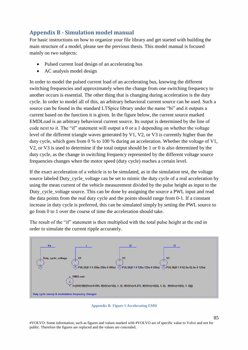
85 #VOLVO: Some information, such as figures and values marked with #VOLVO are of specific value to Volvo and not for
public. Therefore the figures are replaced and the values are concealed.
Appendix B - Simulation model manual For basic instructions on how to organize your file library and get started with building the
main structure of a model, please see the previous thesis. This model manual is focused
mainly on two subjects:
Pulsed current load design of an accelerating bus
AC analysis model design
In order to model the pulsed current load of an accelerating bus, knowing the different
switching frequencies and approximately when the change from one switching frequency to
another occurs is essential. The other thing that is changing during acceleration is the duty
cycle. In order to model all of this, an arbitrary behavioral current source can be used. Such a
source can be found in the standard LTSpice library under the name “bi” and it outputs a
current based on the function it is given. In the figure below, the current source marked
EMDLoad is an arbitrary behavioral current source. Its output is determined by the line of
code next to it. The “if” statement will output a 0 or a 1 depending on whether the voltage
level of the different triangle waves generated by V1, V2, or V3 is currently higher than the
duty cycle, which goes from 0 % to 100 % during an acceleration. Whether the voltage of V1,
V2, or V3 is used to determine if the total output should be 1 or 0 is also determined by the
duty cycle, as the change in switching frequency represented by the different voltage source
frequencies changes when the motor speed (duty cycle) reaches a certain level.
If the exact acceleration of a vehicle is to be simulated, as in the simulation test, the voltage
source labeled Duty_cycle_voltage can be set to mimic the duty cycle of a real acceleration by
using the mean current of the vehicle measurement divided by the pulse height as input to the
Duty_cycle_voltage source. This can be done by assigning the source a PWL input and read
the data points from the real duty cycle and the points should range from 0-1. If a constant
increase in duty cycle is preferred, this can be simulated simply by setting the PWL source to
go from 0 to 1 over the course of time the acceleration should take.
The result of the “if” statement is then multiplied with the total pulse height at the end in
order to simulate the current ripple accurately.
Appendix B- Figure 1 Accelerating EMD

86 #VOLVO: Some information, such as figures and values marked with #VOLVO are of specific value to Volvo and not for
public. Therefore the figures are replaced and the values are concealed.
The AC analysis is far simpler. What is required for it to work is to exchange the pulsed
current loads which are to be active in the analysis for AC sources and remove the others. An
AC source is a simple current source which can be set to perform a sweep across all
frequencies in order to see if any stand out. To do so, no particular function needs to be used,
but the AC Amplitude in the AC analysis window to the right in the figure below has to be set
to 1. This allows for the current source to be controlled by the operational directive. An
example of such can be seen in the second figure below.
When all is modeled properly, simply click Simulate as usual. Then click the nodes of the
different components to get the results presented in this report.
Appendix B- Figure 2 The AC source setup
Appendix B- Figure 3 Current source and operational directive used in the AC analysis