DC Motor-Clutch-Generator Control Workstation

Senior Project Report

Simon Benik and Adam Olson

Advisor: Dr. Gary Dempsey

EE451 Senior Capstone Project

16 May 2006

Abstract:

This senior project is the design of a motor-clutch-generator controls workstation. The plant of the system is the motor-clutch-generator. The motor will be attached to an electrical clutch, with the other end of the clutch being attached to another DC motor, which will act as a DC generator-load disturbance. The clutch can be engaged and disengaged such that the plant will change, and the controller must be able to compensate for these changes. There is also a resistor that can be applied to the generator to vary the load even more. This plant is controlled with software that is implemented on the EMAC 80515 development board using a mixture of assembly and C programming language programming. Also, non-linear modeling techniques are used to create an accurate simulation model of the physical system in Simulink. Interfacing between Simulink and the controller is accomplished.

Table of Contents

Introduction ……………………………………………………….…Page 1

System Description……………………………………………….…..Page 2

Project Subsystems…………………………………….……...…Pages 2 - 4

Preliminary Work as of First Semester………...….……......…Pages 4 – 7

Final Work Software…………………………………………….……..Pages 8 - 9

Hardware...……………………………………..…….….Pages 9 - 10 Modeling………………………………………………..Pages 10 - 13

Model Analysis….……………………………….…......Pages 13 - 18 Controller Designs………………………...……….…..Pages 19 - 21 Conclusion and Recommendations……………………...…………Page 22 Appendix I

List of Sources…………………….…………………………Page 23

Appendix II Equipment …………………………...………………………Page 23

Appendix III Project Specifications……………………………………Pages 23-25

Appendix IV Hardware schematics…………………………………Page 25

Table of Contents (Continued)

Appendix V Matlab controller/model code……………...…………..Page 25 – 28 Appendix VI

Known Bugs……………………………………………...Page 28 NOTE: Appendixes A, B, C, and D can be located on the CD included with this report. Appendix A Mini-project Material Appendix B Software Code Appendix C Diagram of Physical System Appendix D Flowcharts

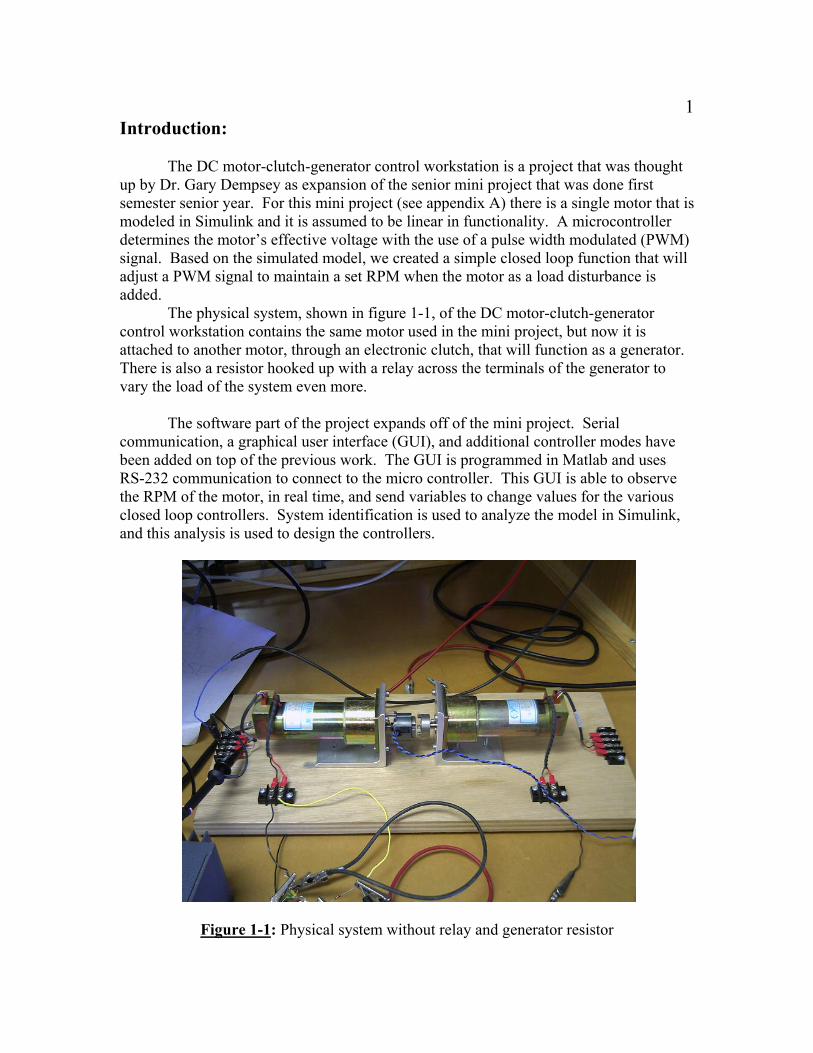
1 Introduction: The DC motor-clutch-generator control workstation is a project that was thought up by Dr. Gary Dempsey as expansion of the senior mini project that was done first semester senior year. For this mini project (see appendix A) there is a single motor that is modeled in Simulink and it is assumed to be linear in functionality. A microcontroller determines the motor’s effective voltage with the use of a pulse width modulated (PWM) signal. Based on the simulated model, we created a simple closed loop function that will adjust a PWM signal to maintain a set RPM when the motor as a load disturbance is added. The physical system, shown in figure 1-1, of the DC motor-clutch-generator control workstation contains the same motor used in the mini project, but now it is attached to another motor, through an electronic clutch, that will function as a generator. There is also a resistor hooked up with a relay across the terminals of the generator to vary the load of the system even more.

The software part of the project expands off of the mini project. Serial communication, a graphical user interface (GUI), and additional controller modes have been added on top of the previous work. The GUI is programmed in Matlab and uses RS-232 communication to connect to the micro controller. This GUI is able to observe the RPM of the motor, in real time, and send variables to change values for the various closed loop controllers. System identification is used to analyze the model in Simulink, and this analysis is used to design the controllers.

Figure 1-1: Physical system without relay and generator resistor

2

System Description:

Goals of the project are:

• A plant controller implemented in C language with the EMAC 80515 development board.

• A user interface that allows for changing control parameters and for motor control; as well as allowing the display of real time operation data.

• Serial communication between the EMAC 80515 development board and a PC using an RS232 serial interface for data sharing.

• Non-linear modeling of the physical system using control theory, Simulink, and Matlab.

• A graphical user interface (GUI) in Simulink for the purpose of easy manipulation of the model for simulation and its data.

The project consists of three primary subsystems. The first subsystem is the

physical system. This includes the DC motor, the electronic clutch, and the DC generator with its load varied by a relay.

The second subsystem is the Simulink and Matlab modeling. This is where a

mathematical model is created based on data collected from the real system. This model is non-linear in order to imitate the real system as best as possible. Additionally, control methods are designed and evaluated in Simulink before they are implemented in the third subsystem. A GUI is created as well for interfacing with the third subsystem over a serial connection.

The third subsystem is the software based controller that is implemented on the

EMAC 80515 development board. This subsystem’s functions are to allow the user to set control parameters, display the physical system’s operation status such as velocity, and also to use control algorithms and feedback data to accurately control the physical system with its PWM signal which will drive the motor. Moreover, the EMAC 80515 development board was programmed to communicate with a PC running Simulink through serial communication. These systems are combined for an overall system block diagram. The Physical Subsystem

The block diagram of the motor-clutch-generator workstation, with subsystems labeled for reference, is shown in figure 4-1. The motor subsystem consists of the Pittman DC motor with its rotary encoder and the hardware used to interface the motor with the EMAC development board. The motor is controlled by the EMAC 80515

3 subsystem using a PWM signal. The speed of the motor is then fed back to the EMAC 80515 subsystem by the rotary encoder, which produces pulses proportional to the speed of the internal shaft of the motor. The interface hardware consists primarily of an H-bridge, which amplifies the PWM signal from 5 Volts to 20 Volts. The clutch subsystem consists of a clutch that is electronically activated and, when activated, is used to couple the motor shaft to the DC generator shaft, thus changing the plant model. The DC generator subsystem is the DC generator and its variable load using a relay. The DC generator is a second Pittman motor. Its load will be determined by a high power rated resistor that is connected to the motor with a relay. The relay is a simple switch that either maintains an open circuit across the terminals of the generator or places a resister between them. The EMAC 80515 Subsystem

The EMAC 80515 subsystem uses a liquid crystal display (LCD) for displaying its interface to the user. The LCD is also used to display real time data of the operation of the physical system. A keypad is used as the primary user input, allowing the user to enter parameters and choose between options. Another element of the EMAC 80515 subsystem is the software-based controller. This controller is used with the feedback from the motor’s rotary encoder to implement a closed loop controller. This closed loop controller is used to control the velocity of the motor. Various control theory methods are explored for the implementation of this controller such as proportional control, proportional-integral-derivative (PID) control, root-locus design, and frequency domain design. The final component of the EMAC 80515 subsystem is the RS232 serial interface. The microcontroller takes the feedback information from the rotary encoder, of the motor, and sends this data to a PC running Matlab and Simulink using the serial interface. This data can be used to analyze the operation of the physical system without heavy use of lab equipment such as the oscilloscope. Also, the microcontroller uses the serial interface to receive command signals from the PC. These command signals include; the speed that the PWM will increase or decrease when their respective buttons are pushed, whether the clutch or generator load is enabled, and various closed loop variables. The command signal will be stored in RAM and will allow the microcontroller to produce complex command signals without the need for implementing an extensive algorithm in the microcontroller code itself. Simulink Subsystem

Finally, the Simulink subsystem consists of Matlab and Simulink software running on a PC. Simulink is used to model the physical system using control block diagram elements and other functions. The model is non-linear, with its parameters determined using the motor data sheets and experimental data. Also, Simulink is used to generate a GUI, for the user to change parameters of the model and other options. Matlab will be used both for actual serial communication programming as well as for storing variables such as command signals and control parameters.

4

Figure 4-1: System Block Diagram

First Semester and Preliminary Work: The preliminary work for this project includes all physical and software components of the “senor mini-project”. Six days of lab were used to gather information and to evaluate the project in the first semester. The physical system was completed by both students. Simon Benik researched serial communication using the UART on the EMAC development board. Progress was made, but more work on serial interfacing was postponed until more issues have been tackled to make best use of the time available. He also improved previous work on the EMAC 80515 development board user interface and has consolidated the code used to generate pulse width modulation signals. He began the high level design of the software. The high level flow chart is shown below in figure 5-1.

5 Adam Olson began modeling the physical system by collecting experimental data

and using it to create models in Simulink. He found the torque of the motor at various speeds and voltages by measuring the current into the motor. Three trials were performed. The types of frictions of a DC motor are shown in figure 6-1.

Figure 5-1: Preliminary High Level Flow Chart.

6

Figure 6-1: Non-linear friction characteristics of a DC motor

With this friction data collected, a non-linear model was created which is shown in figure 6-2.

Figure 6-2: Non-linear friction model of DC motor control system in Simulink

Non-Linear Modeling

• Static Friction • Coulomb Friction

• Viscous Friction • All Frictions Combined

7

With this model, the physical system can be simulated. Many parameters of the system can be measured in the simulation such as torque, velocity, current, and voltage. For example, the graph in figure 7-1 shows how closely the simulation models the actual system by displaying both experimental results and simulated results of the system’s current with respect to velocity.

Figure 7-1: Experimental results vs. simulated results of the physical system

The green plot is what the motor’s current would be in the model if it were

modeled using only linear techniques. The non-linear model is an almost perfect match to the experimental system, and a vast improvement over the linear model.

8 Second Semester Results: The second semester work is sectioned off into software components, modeling, controller design, and hardware. Software: All project specifications have been accomplished except for the + 5 RPM accuracy, and some closed loop control functionality, because of time restraints. The interface on the EMAC is complete. The user can view real-time PWM and RPM measurements, and also set various features such as; poll timing for PWM adjustment, RAM data storage timing, store incoming RPM to RAM, and send RPM speed to computer in real-time or from RAM. RAM Data Storage The EMAC kit can store 255 points of RPM data to RAM when the ‘F’ key is pressed on the keyboard. The data is stored in external memory at location 9500h. These points can be taken at an interval of anywhere between 1 and 255ms apart. The default timing for this is one point taken every 4ms but can be adjusted by the user in either the EMAC interface or the GUI in Matlab. Serial Communication

The EMAC kit will send and receive data through the serial connection to the computer. When ‘B’ is pressed the micro-controller will send the RPM data and the recording timing stored in RAM to the computer. If the computer is waiting for the data (with GUI or test.m) it will graph the recorded data in Matlab with correct axis. When ‘E’ is pressed the micro-controller will send RPM data in real-time mode. Through experimentation we found sending every 2ms is the fastest possible speed without error. If the GUI is set for real-time or the program realtime.m is running while the system is in this mode Matlab will graph the RPM data in real-time, 500 points 2ms apart at a time.

When the computer ever sent data to the EMAC it would send two bytes. The first byte would be the location byte that would tell the EMAC the type of command. Some examples of commands would be: RPM set speed, poll timing, and enable or disable clutch. The second byte sent would be the actual value for a register.

The serial communication between the EMAC and the computer using RS232 was successful and is now able to transmit and receive information. Though there was a problem in the communication where the highest bit was never able to be sent or received, a software fix was implemented to fix the error. This serial communication is directly interfaced with Matlab and several programs have been created to make use of the communication. All programs can be found in appendix B, along with programs for Matlab.

9 Graphical User Interface (GUI) In Matlab, a GUI (see figure 9-1) was created to incorporate all the functionality

of the various programs created. Due to time restraints the GUI is not finished. It can function in both real-time mode and graph from RAM and can send variables when in real-time mode. Also, it will crash if button is pressed to display a graph from RAM.

Figure 9-1: Graphical User Interface (GUI)

Hardware: The entire hardware system can be seen in figure 10-1. The schematic of this system is included in appendix C. This system includes two Pittman DC motors, electronic clutch, H-bridge, relay, 2 switches, 7486 (XOR) chip, a transistor, and several resistors, diodes, and capacitors. The 2N222A transistor is used as a switch for the interface between the EMAC 80515 development board and the clutch so that the clutch can be controlled through software. Likewise, the relay is used to interface the software to the external load of the generator so that it can be switched as part of the plant during operation.

10

Figure 10-1: Entire Physical System without EMAC kit Modeling: As mentioned in the preliminary work section, a nonlinear physical model of the motor was found experimentally with the nonlinear elements being static friction torque and coulomb friction torque. Also, the viscous friction torque was found to be nonlinear, possibly because of an unknown internal effect inside the motor; the viscous friction torque leveled out along curve as velocity increased.

Static Friction Torque Static friction torque is determined by slowly increasing the voltage input

to the motor’s terminals, and indirectly measuring the current flow using a 1Ω resistor in series with the power supply and motor terminal and measuring the voltage across the resistor. Current increased to a maximum value of 89.2mA and then dropped significantly (the motor shaft began to move). The torque required to overcome this friction is directly proportional through the Kt constant, so friction torque was then calculated using a KT value of 58.2x10-3 (N-m /A):

Static Friction =Static Current x KT = 0.0892A x 58.2x10-3 (N-m/A) = 5.17982x10-3 N-m

11 Coulomb Friction Torque

Coulomb friction torque was determined as the drop off from static friction torque to the offset friction inherent at shaft velocity > 0 rad/sec. Just as the voltage input setting to overcome static friction torque is reached, the friction of the motor will be almost entirely coulomb friction torque, with the only caveat being that the Stribeck effect (a nonlinear friction present at low velocities) was neglected. At this point, the current was again measured to be a value of 48mA. Using the Kt constant, the coulomb friction torque of the motor is below:

Coulomb Friction Torque = 0.048A x 58.2x10-3 (N-m/A) = 2.77x10-3 N-m

Viscous Friction

Viscous friction torque was found by performing a voltage sweep across the motor’s operating voltage. At each voltage, the steady-state current was recorded as well as the internal shaft velocity of the motor using the rotary encoder. After all data was taken, the viscous friction torque was plotted and appeared to be non-linear. A cubic equation fit was used in Matlab to fit a curve to the viscous friction data collected. The following equation describes the viscous friction in relation to velocity, with velocity = ω (rad/sec):

Viscous Friction Torque = 1.0751x10-11 (N-m/(rad/sec)) x ω3 - 1.7739x10-8 (N-

m/(rad/sec)) x ω2 + 1.205x10-5 (N-m/(rad/sec)) x ω Note: This viscous friction torque is offset by the coulomb friction.

The same procedure was then used to measure the friction parameters for when the clutch was attached to the shaft, both in the engaged and disengaged states, since frictions differed between these states. The motor’s frictions were subtracted from these measurements to obtain just the frictions of the clutch. The DC generator friction was set equal to the motor’s frictions, since these are equivalent systems. The static and coulomb friction torques of the states are shown in table 11-1, and the viscous friction torques of the states are shown in table 11-2. Table 11-1: Static and coulomb friction torques of the plant in different states

Motor/DC Generator Clutch Disengaged Clutch Engaged

Static Friction Torque 5.17982 x 10-3 N-m 7.9152 x 10-4 N-m 6.8967 x 10-3 N-m

Coulomb Friction Torque 2.77x10-3 N-m 3.942 x 10-4 N-m 2.8518 x 10-3 N-m

Table 11-2: Viscous friction torques in different states with relation to internal shaft ω

Motor/DC Generator 1.0751x10-11 (N-m/(rad/sec)) x ω3 - 1.7739x10-8 (N-m/(rad/sec)) x ω2 + 1.205x10-5 (N-m/(rad/sec)) x ω

Clutch Disengage -3.411x10-9 (N-m/(rad/sec)) x ω2 + 1.8787x10-6 (N-m/(rad/sec)) x ω

Clutch Engaged 3.6899x10-9 (N-m/(rad/sec)) x ω2 - 4.785x10-6 (N-m/(rad/sec)) x ω

12

In summary, first the frictions of the motor alone were measured, then the frictions of the motor with the clutch attached were measured, and finally the motor with the clutch engaged and coupled to the DC generator. This method allowed for the separate component frictions to be measured. In the model they have been cascaded, such that the first friction block must be overcome before each following friction can be added to the total friction. The motor-clutch-generator system is represented as a circuit to perform analysis in order to derive a block diagram of the system. Analogous mechanic’s equations are solved using circuit analysis with Kirchoff’s laws, where friction and inertia are represented as resistance and capacitance. The friction is represented in Matlab m-file code because of the non-linearity such that they are extracted from the friction-inertia transfer function. What is left of the transfer function is the inertia of the components. Inertia of the clutch is marginal such that it can be neglected. The motor’s datasheets were used to find the inertia. The transfer functions derived for the inertia from circuit analysis are below:

Motor, Clutch, and Generator Inertia = s61006.7

1−×

Motor and Clutch Inertia = s61012.14

1−×

Using the equations derived in the circuit analysis, a more complex system model can be represented in Simulink. This model is shown in figure 13-1. The input voltage is converted into a frequency dependent current through the internal motor impedance transfer function, and this current is combined with the opposing current of the DC generator to give the resultant current used to drive the load. This current is then converted into torque using the motor’s KT conversion factor and is fed into the nonlinear friction m-file blocks. When these friction torques are deducted from the torque generated by the motor-generator torque, the resulting torque is combined with the lumped inertia transfer function of the system, resulting in a velocity ω output. The ω signal is fed back into the nonlinear friction m-file blocks, because the code in these blocks use the ω information to determine the nonlinear friction. This ω is also sent in a feedback loop to the motor’s input voltage through a KM conversion (equal to KT in SI units) which represents the motor’s back EMF. This back EMF is also sent into another loop to the DC generator, which is sent into a time delay block to account for the motor’s inherent time delay that was measured looking at the plant’s transient waveform’s experimentally. The back EMF is then converted to current through the DC generator’s internal impedance transfer function. This transfer function’s resistance value is dependent on the generator’s external load on its terminals. With a load of 0Ω (terminals shorted), this value becomes 3.91Ω which is the internal resistance of the motor’s windings. With a load of ∞ Ω (terminals open), the load becomes ∞, however, it is

13 practical to set to 3.91Ω+500Ω for simulation-computation-time considerations. The resulting current is the current flowing in the generator and represents the torque opposing the motor’s torque. The switches are added to allow for simulation of the system in the different clutch states: clutch removed, clutch attached and disengaged, and clutch engaged with generator coupled.

Figure 13-1: Motor-Clutch-Generator Plant Simulink Nonlinear Model

Validation of the Simulink Model: With the model created, it is important to validate its accuracy to the real system. To do this, both steady-state and transient measurements are taken of the real system and the Simulink model, and then these measurements are compared. Also nonlinear parameters are confirmed. In the experimental data, on average of three trials, the entire system coupled requires about 1.25 volts to overcome the static friction of the system. The Simulink figure 14-1 shows the voltage required to overcome the nonlinear friction of the simulation, 1.216 volts, which is very close to the real system’s 1.25 volts.

14

Figure 14-1: Nonlinear characteristics in model simulation nearly

identical to those of the real system.

Figure 15-1 shows both the transient and steady-state characteristics of the real system and simulated model of the system. This simulation comparison is made before time delay is added to the model, so the experimental time delay offset is removed. The blue and red signals are from the experimental measurements, and can be seen to be very noisy, however, their average values are extremely close to the simulated values, and the transient response of the step inputs of both the simulation and the real system are nearly identical aside from some loading of the power supply in the real system. The time constant of this response is measured to be 0.0147 seconds from the simulated signal, and time delay is neglected in this calculation. The attenuation of the input DC motor voltage to output DC generator voltage is due to an energy drop in the internal system. This creates a voltage drop across the various components such that not all voltage is transferred from the input to output.

15

Figure 15-1: Experimental and Simulated step response comparison of

steady-state and transient behavior. Frequency Response of the Plant: The model of figure 14-1 is used to determine the frequency response of the plant. Because of noise and other practical inefficiencies of measuring the real system, and because of the close match of the model to the real system, it is easier to measure the frequency response of the model.

A sine wave frequency sweep input is used to find the frequency response of Vininternalω

.

The input sine wave has to be biased and has to be large enough to overcome the nonlinear frictions of the system. The recorded data is plotted and a second-order approximation of the transfer function is derived. The frequency response of the second-order approximation is plotted on top of the measured frequency response of the model in figure 16-1 to show the consistency of the two.

16

Figure 16-1: Frequency response of the plant model (red) and the

second-order approximation (blue). The second-order approximation is accurate both for magnitude and phase, so it is used to represent the transfer function of the plant (motor-clutch-generator coupled):

Vininternalω

= ⎟⎠⎞

⎜⎝⎛ +⎟⎠⎞

⎜⎝⎛ + 1

9501

65

557.16SS

Hybrid Digital-Analog Plant-Control System: With the non-linear plant reduced to a simple second-order transfer function, the rest of the system including the EMAC 80515 development board and H-bridge circuitry that drives the plant can be included into an overall system block diagram shown in figure 17-1.

17

Figure 17-1: The hybrid-digital-analog control system

Neglecting all nonlinear saturation blocks of the PWM and H-bridge, the Open-loop transfer function of figure 17-1 is:

⎟⎠⎞

⎜⎝⎛ +⎟⎠⎞

⎜⎝⎛ +

×=×××××

1950

165

3589.0SSGhonversionSoftwareCoderRotaryEncoGpHbridgePWMGc

This transfer function is used in Matlab (see appendix V) to plot the open-loop frequency response including the zero-order hold of the PWM with a sampling period of 1ms by using the c2dm command with the ‘zoh’ parameter. Again, an approximate transfer function was matched to this resulting frequency response. A third-order approximation had to be used to account for the extra phase added to the system by the zero-order hold. The frequency response of the transfer function using Matlab dbode command and its third-order approximation are shown in figure 18-1. Phase and magnitude curves match up nicely, so this third-order transfer function can be used for controller design in the s-plane:

⎟⎠⎞

⎜⎝⎛ +⎟⎠⎞

⎜⎝⎛ +⎟⎠⎞

⎜⎝⎛ +

=×××××1

18001

8501

60

0146.0SSS

nversionSoftwareCoderRotaryEncoGpHbridgePWMGc

The corresponding root-locus is shown in figure 18-2. This plot is used to verify the system and can be used to calculate overshoot and gain, however, controller design is primarily done using frequency response for this system.

18

Figure 18-1: Frequency response of open-loop system both with c2dm

‘zoh’ (blue) and third-order approximation (green).

Figure 18-2: Root locus of the open-loop system in the z-domain with two poles. A

gain of 2750 in Gc is the limit for stability in the system.

19 Controller Design: Proportional Controller

Using the third-order open loop transfer function, a phase margin spec of 55º is chosen for the controller design. The crossover frequency, ωc, is found using an exact phase equation:

⎟⎠⎞

⎜⎝⎛−⎟

⎠⎞

⎜⎝⎛−⎟

⎠⎞

⎜⎝⎛−=°−=°+°−= −−−

1800tan

850tan

60tan12555180 111 ccc

cωωω

β

where the inverse trig addition identity is used to solve for ωc:

( ) ( ) ⎟⎟⎠

⎞⎜⎜⎝

⎛−+

=+ −−−

αββαβα

1tantantan 111

The crossover frequency is determined to be:

( )sec/18.473 radc =ω

The D/A cost for this controller will be 28.1318.473

10002==

πωω

c

s , where ωs is

the sampling frequency. This is a reasonable cost considering ωs is already determined by the software design already in place.

Solving for proportional gain Kp with the ωc design choice, the proportional controller gain Kp is 644. This gain is added into the Matlab code, and the new open-loop frequency response shows that, indeed, a Kp value of 644 results in a ωc of approximately 473.18 rad/sec and a phase margin of 55º. Controller implementation is done simply by multiplying the difference in set pulses and rotary encoder pulses by this gain value, however there are limitations in the microcontroller implementation that results in saturation of the PWM signal. A more thorough software design is necessary to implement this controller. The simulated closed-loop system 100 RPM command signal step response is shown in figure 20-1. Response time is fast which is good, but there is overshoot and steady state error as expected. Because of this error, we decided to sacrifice the speed of this controller and design a more complex PI controller.

20

Figure 20-1: Proportional Controller Closed-Loop System Step Response (100

RPM step command signal) Proportional-Integral Controller Again, the third-order open loop transfer function was used for controller design. The phase margin spec was reduced to 50º because the PI controller creates a slower system inherently with the integrator, so we tried to let the system be faster by sacrificing 5º of stability. Using a Kp gain block and a Ki/S block in parallel, the controller transfer function is determined to be: Or The z-domain transfer function is determined using the bilinear transformation of Gc(s) (Tustin method). With this controller the crossover frequency is smaller than that of the proportional controller by an order of magnitude, and the D/A converter cost is high; however, this is not a problem for this system with a fixed sampling period: So the system is slower, but as seen in figure 21-1, steady-state error has been reduced to 0 for the step command. Using the Gc(Z) transfer function, a difference equation for programming the EMAC 80515 development board system is:

⎟⎟⎟⎟

⎠

⎞

⎜⎜⎜⎜

⎝

⎛⎟⎠⎞

⎜⎝⎛ +

=S

S

sGc1

5004658

)( ⎟⎠⎞

⎜⎝⎛

−−

=1

987.6645.11)(zzzGc

( )sec/75.51 radc =ω

11 987.6645.11 −− −+= nnnn rryy

4.12175.51

10002==

πωω

c

s

21

This equation is not easy to implement on the 8-bit microcontroller, so rounding can be done, but the affect this rounding has on the controller could result in an insufficient controller depending on how much room there is to work with in the z-domain.

Figure 21-1: Proportional-Integral Controller Closed-Loop System Step Response (100 RPM step command signal)

Overshoot of the simulation is approximately 30%, but the design equations predict overshoot to be about 16%, so the nonlinearities of the Simulink model do have a large impact on the frequency response of the system.

22

Conclusions and Recommendations: The project was complete with all specifications made. The modeling and simulation is accurate. The proportional and integral controllers are functional. The software programming successfully interfaced the computer with the system. Due to time restraints, there are still a few bugs in the system that still needs to be corrected (Appendix VI). Recommendations This control workstation can be used to as a benchmark to compare future “mini-projects.” Several sections of this project can be added into the “mini-project” to increase the difficulty for students. Additional and more complicated controllers can be designed and implemented with this system. More data can be sent from the microcontroller to the computer, such as PWM values.

23 Appendix I – List of Sources: 1) Dr. Gary Dempsey. Advisor in all aspects of research and design. 2) Pittman Motor Application Notes. 2000.

http://blackboard.bradley.edu/courses/1/EE451_01_06FA/content/_455117_1/220000ALL.pdf

3) Clutch Product Information with Data Sheet. Reell Precision Manufacturing.

2004. http://www.reell.com/products/ec15.htm

4) Functional Requirements and Performance Specs, Dr. Gary Dempsey, EE450 Electronic Product Design. http://blackboard.bradley.edu/@@cb65f20b7d29e2f11466cc12ddf1fae5/courses/1/EE450_01_06FA/content/_390634_1/mini_project_figures_diagrams_06.doc

Appendix II – Equipment: The equipment list only includes main components of the system. The list is below in table 20-2. Table 20-1: Equipment List

Parts Quantity EMAC 80515 Development Board 1 HP 30V Power supplies 2 LMD18200 H-bridge Motor Controller 1 Pittman DC Motors 2 Reell EC15 Spring Clutch 1 Relay 1 Matlab and Simulink Software on a PC 1

The HP 30V power supplies will be used to power the H-bridge, which in turn supplies the DC motor, and also to power the electric clutch. The H-bridge is used to control the motor by increasing the voltage of the PWM signal from the EMAC board. The DC motors and the clutch are part of the physical system, and the 5.6 Ohm potentiometer serves as the variable load for the DC generator. Appendix III – Project Specifications:

With this project, there are a wide number of specifications that can be made. The specifications have been organized below so that each pertains to a specific subsystem of the project. Many specifications have not been completed because lack of time (shown with *); however, these have been identified, regardless of real figures. The specifications are as follows:

24 Motor subsystem:

1) Operation temperature: 0 to 40°C 2) Power supply voltage: 30V DC 3) Maximum torque: 67.1x10-3 N-m (continuous) 4) Analog circuit-hardware protection 6) Closed-Loop Operating Range: Bias ~420 RPM with ± 300 RPM limits

Clutch subsystem: 1) Power supply voltage: 12V DC 2) Maximum torque: 1.7 N-m (continuous) 3) Operating direction: clockwise DC generator subsystem: 1) Maximum load: DC Generator with 0 Ω load (shorted terminals) 2) Load power rating: 4 W 3) Maximum torque: 67.1x10-3 N-m (continuous) 4) Variable load by way of software control 5) Variable load by way of manual user control 6) Operating direction: counter-clockwise EMAC 80515 subsystem:

1) Two line LCD main display: Measured parameters on line 1 including RPM, torque*, etc. Control parameters on line 2 including command RPM, PWM generation duty cycle

2) Secondary display of menu, which consists of operation mode selection and parameter selections

3) Display refresh rate: 0.5 seconds 4) Motor Velocity: display accuracy + 5* RPM (only achieved + 10) 5) PWM: period waveform (1 millisecond), variable duty cycle (0 to 100% in

0.2% or less increments), display accuracy: + 0.2% 6) Serviced every 40 ms (default), keypad selectable from 5 to 250ms 7) Proportional, proportion-integral, and proportion-integral-derivative

controller implementations (more methods optional)

8) Partial RS232 serial interface with use of EMAC 80515 development board UART with rate of 9600 baud.

9) Simulink operation mode: Ability to send physical system data and receive command signals to store in RAM.

10) Digital controller sampling period of 1ms

Simulink subsystem: 25

1) System model: Open-loop and closed-loop modeling of the physical system

2) Non-linear modeling: Non-linear modeling for the static, Coulomb, and viscous frictions of the motor, and for the clutch subsystem non-linearity.

3) GUI for changing parameters of the model and other options 4) Serial communication with EMAC 80515 development board for sending

command signal variables and for receiving physical system data 5) Method for comparing and analyzing the physical system with the

modeled system, with the goal of method realized in real time Appendix IV – Hardware Schematics:

Fig. 22-1: H-bridge circuitry used to control the motor and interface with the

microcontroller. Appendix V – Matlab Code: The following code is contained in the m-file blocks of the system plant model, which makes up the nonlinear frictions. Motor nonlinear friction m-file code: function y = Motor_Friction(Tin, vel) % This block supports an embeddable subset of the MATLAB language. % See the help menu for details. %Ts = 0.0051798; % Static Friction (N*m).. 89.2mA * 58.2e-3*N*m/A = 0.0034877 N*m Ts = 0.0055872; % adjusted Ts %Tc = 0.0027743; % Coulomb Friction(N*m).. 48mA * 58.2e-3*N*m/A = 0.0018768 N*m Tc = 0.002541594; % adjusted (tuned) Tc

26 Tb= (58.2e-3)*((1.8472e-10)*(vel^3)- (3.048e-7)*(vel^2) + (0.000207)*vel); %Tc omitted as separate; if (vel~=0) y = Tin - (Tc*sign(vel) + Tb); elseif (vel == 0 && Tin < Ts) y=0; else y = Tin - Ts*sign(Tin); end Clutch nonlinear friction m-file code: function y = Clutch_Friction(engage, Tin, vel) % This block supports an embeddable subset of the MATLAB language. % See the help menu for details. if(engage == 2) Ts = 0.0068967; % Static Friction (N*m).. 207.5mA-89mA=118.5mA * 58.2e-3*N*m/A = 0.0068967 N*m %Ts = 0.0; % adjusted Ts Tc = 0.0028518; % Coulomb Friction(N*m).. 97mA-48mA=49mA * 58.2e-3*N*m/A = 0.0028518 N*m %Tc = 0.002541594; % adjusted (tuned) Tc Tb= (58.2e-3)*((6.346e-8)*(vel .^2) - (0.08221e-3)*(vel)); if (vel~=0) y = Tin - (Tc*sign(vel) + Tb); elseif (vel == 0 && Tin < Ts) y=0; else y = Tin - Ts*sign(Tin); end elseif (engage == 1) Ts = 0.00079152; % Static Friction (N*m).. 102.6mA-89mA=13mA * 58.2e-3*N*m/A = 0.00079152 N*m %Ts = 0.0055872; % adjusted Ts Tc = 0.0003942; % Coulomb Friction(N*m).. 54mA-48mA=6mA * 58.2e-3*N*m/A = 0.0003942 N*m %Tc = 0.002541594; % adjusted (tuned) Tc Tb= (58.2e-3)*((-5.86e-008)*(vel^2)+ (3.228e-005)*(vel)); if (vel~=0) y = Tin - (Tc*sign(vel) + Tb); elseif (vel == 0 && Tin < Ts) y=0; else y = Tin - Ts*sign(Tin); end else y = Tin; end

27 Generator nonlinear friction m-file code: function y = Generator_Friction(coupled,Tin, vel) % This block supports an embeddable subset of the MATLAB language. % See the help menu for details. if (coupled == 2) %Ts = 0.0051798; % Static Friction (N*m).. 89.2mA * 58.2e-3*N*m/A = 0.0034877 N*m Ts = 0.0055872; % adjusted Ts %Tc = 0.0027743; % Coulomb Friction(N*m).. 48mA * 58.2e-3*N*m/A = 0.0018768 N*m Tc = 0.002541594; % adjusted (tuned) Tc Tb= (58.2e-3)*((1.8472e-10)*(vel^3)- (3.048e-7)*(vel^2) + (0.000207)*vel); %Tc omitted as separate; if (vel~=0) y = Tin - (Tc*sign(vel) + Tb); elseif (vel == 0 && Tin < Ts) y=0; else y = Tin - Ts*sign(Tin); end else y = Tin; end The following code is used to obtain a frequency response of the hybrid control system using the PWM zero order hold: % I use this code to get my zero order hold phase lag included with the % control tool box. My final result is the z-transform transfer function % of the closed-loop and open-loop systems with proportional control Kp. Kp =1; %controller gain numf = Kp *.00542*4*16.557; %forward path numerator denf = [1.6194e-5 .016437 1]; % forward path denominator numfb = 81.5 * .001; % feedback path numerator denfb = 1; % feedback path denominator [numfd, denfd] = c2dm(numf, denf, .001, 'zoh'); % z-transform using zoh method to get phase lag from zoh in the system (the pulse width modulation) [numfbd, denfbd] = c2dm(numfb, denfb, .001, 'zoh'); %not really necessary to take z-transform of the feedback path since it is a constant so same in s-plane as z-plane sysd = tf(numfd, denfd); sysfbd = tf(numfbd, denfbd); [sys] = feedback(sysd, sysfbd); % sys is my closed-loop system in z-transform

28

[numdcl, dendcl] = feedback(numfd, denfd, numfbd, denfbd); % separated closed loop numerator and denominator figure; dbode(numdcl, dendcl, .001); % z-domain "bode" plot using .001 sampling period figure; dstep(numdcl, dendcl, 30); % step % ROOT LOCUS AND OPENLOOP numOL = Kp*.00542*4*8.28*81.5*.001; denOL = [1.6194e-5 .016437 1]; [numOLd, denOLd] = c2dm(numOL, denOL, .001, 'zoh'); %z-plane open loop numerator and denominator figure; dbode(numOLd, denOLd, .001); % z-domain "bode" plot using .001 sampling period k = 0:1:3000; figure; axis('square'); zgrid('new'); rlocus(numOLd, denOLd,k); %figure; axis('square'); zgrid('new'); rlocus(numOLd, denOLd); Appendix VI – Known Bugs:

In the Matlab GUI there is a glitch where the “Display from RAM” button won’t function if the GUI is already running in real-time mode.

In the final build of the EMAC program trying to record data into ram will crash

the system. The program somehow has the closed loop flag set when recording into ram even though it never interacts with the closed loop registers. Occasionally, interface between Matlab and the microcontroller will be freeze. This error will lock up the serial port within the Matlab program. The program will not be able to be closed and a complete system restart is necessary to use the serial interface again. The interface on the EMAC will not receive any Kp input value from the keypad. The Kp can still be changed through the use of the Matlab GUI.