david smith and andy newell - homepages.warwick.ac.uk

Measuring Vibrations from Video Feeds ESGI130

Measuring Vibrations from Video Feeds

Problem presented by

David Smith and Andy Newell

Ministry of Defence

ESGI130 was jointly hosted byUniversity of Warwick

Smith Institute for Industrial Mathematics and System Engineering

i


Report author

Ed Brambley (University of Warwick)

Executive Summary

By using a high-speed camera, researchers at MIT in 2014 where ableto recover human speech from videos of minute vibrations of objectsin a room. For example, in one experiment a 2,200fps camera waspositioned outside a room behind sound-proof glass, videoing an emptycrisp packet on the floor inside the room, while a researcher shouted“Mary had a little lamb” at the crisp packet. By detecting minuteoscillations of the crisp packet of 1µm (0.001 mm), and using hours ofcomputer processing, a ten second audio clip could be produced thatwas recognisably “Mary had a little lamb” in an American accent.

The purpose of this study group was to investigate whether this tech-nique could be used in practice, with emphasis on the recovery of intel-ligible speech from a video feed of a room. During the week, the groupinvestigated several aspects of the problem, including:

• how much an object vibrates due to sound;

• what can be done to maximize the vibration;

• how the MIT technique detects minute vibrations in videos;

• what affects the quality of the resulting recording; and

• how good a recording is needed for intelligible speech.

It was discovered the MIT experiments would not have recovered intel-ligible speech from an ordinary conversation; their success depended onloud sounds and prior knowledge of “Mary had a little lamb”. Cameravibrations were also ignored by MIT; these are expected to be signifi-cant, but the technique could be adapted to be resilient to them. Otherpossibilities for enhancing their technique, by exploiting resonances orreflections, are discussed in the report. A high-speed low-noise cam-era is essential, and any existing video footage (such as from CCTV) isunlikely to be of sufficient quality. Further experiments with high-endhigh-speed cameras are needed to assess the feasibility of the techniquein practice.

Version 1.0October 9, 2017

iv+23 pages

ii


Contributors

Ed Brambley (University of Warwick)Helen Fletcher (University of Oxford)

Roger Hill (University of Warwick)Ifan Johnston (University of Warwick)

Jessie Liu (University of Warwick)Robert MacKay (University of Warwick)

James Mathews (University of Cambridge)John Ockendon (University of Oxford)Bernard Piette (Durham University)

iii


Contents

1 Introduction 11.1 Sound during conversations . . . . . . . . . . . . . . . . . . . . . . 1

2 Acoustic excitations of thin plates 22.1 Sound exciting an infinite elastic beam . . . . . . . . . . . . . . . . 32.2 Resonances of a 2D rectangular plate . . . . . . . . . . . . . . . . . 72.3 A forced elastic plate . . . . . . . . . . . . . . . . . . . . . . . . . . 82.4 Interaction between sound and a resonating object . . . . . . . . . . 10

3 Reflection from a bending mirror 12

4 Detecting motion from video 134.1 Rolling shutter . . . . . . . . . . . . . . . . . . . . . . . . . . . . . 154.2 Quality of detected motion and noise . . . . . . . . . . . . . . . . . 17

5 Intelligible speech 18

6 Conclusion 20

A Appendices 22A.1 Recognising speech from a noisy background . . . . . . . . . . . . . 22

References 23

iv


1 Introduction

(1.1) In their 2014 paper, MIT researchers Davis et al. [1] demonstrated the re-covery of the sound in a room from a video of some objects present in theroom. The idea is that sound is the vibration of the air in the room, whichcauses minute vibrations of objects in the room exposed to that sound. Onecan then attempt to detect these vibrations from a high-speed video of theobjects, and use motion-enhancement signal processing techniques developedin the same laboratory [7] to extract the audio. The aim of this report is toinvestigate the feasibility of using this technique to extract intelligible speechin practical situations.

(1.2) Section 2 of the report analyses the vibration of simple objects, such as theones used by Davis et al. [1], in order to model the amplitude of vibration asa function of the size and material properties of the object and the amplitudeand frequencies of the sound. In addition to giving ballpark figures of whatsort of equipment would be needed to detect the vibrations, one other aimof this modelling is to determine the ideal properties that an object wouldhave in order to be used as a visual microphone. One novel possibility isto gain greater sensitivity to motion by looking at reflections in an object,rather than the object itself; this is considered further in section 3.

(1.3) Section 4 describes the earlier work from the MIT lab on which the recoveryof sound is based. Wadhwa et al. [7] developed a technique to analyse videoand enhance the motion shown in the video in a particular frequency range.This is how Davis et al. [1] were able to detect the tiny motion of objectsdue to sound.

(1.4) Section 5 investigates what is required for a recording of speech to be intel-ligible. This also gives ballpark figures on what frequencies and noise levelsare needed in practice.

(1.5) Finally, section 6 summarizes the results in this report, and suggests furtherlines of inquiry.

1.1 Sound during conversations

(1.6) The human voice consists of frequencies ranging from 80 Hz to 4 kHz ex-cluding sibilants. In telephony, the voice band is approximately 300 Hz to3.4 kHz1, with the missing information below 300 Hz perceived as a missingfundamental2. Sound restricted to the voice band is noticeably telephone-like, but is none-the-less fully intelligible.

1http://en.wikipedia.org/wiki/Voice_frequency

2http://en.wikipedia.org/wiki/Missing_fundamental

1

http://en.wikipedia.org/wiki/Voice_frequency

http://en.wikipedia.org/wiki/Missing_fundamental


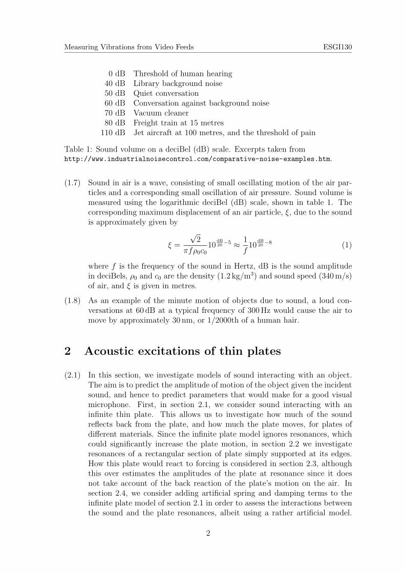
0 dB Threshold of human hearing40 dB Library background noise50 dB Quiet conversation60 dB Conversation against background noise70 dB Vacuum cleaner80 dB Freight train at 15 metres

110 dB Jet aircraft at 100 metres, and the threshold of pain

Table 1: Sound volume on a deciBel (dB) scale. Excerpts taken fromhttp://www.industrialnoisecontrol.com/comparative-noise-examples.htm.

(1.7) Sound in air is a wave, consisting of small oscillating motion of the air par-ticles and a corresponding small oscillation of air pressure. Sound volume ismeasured using the logarithmic deciBel (dB) scale, shown in table 1. Thecorresponding maximum displacement of an air particle, ξ, due to the soundis approximately given by

ξ =

√2

πfρ0c010

dB20−5 ≈ 1

f10

dB20−8 (1)

where f is the frequency of the sound in Hertz, dB is the sound amplitudein deciBels, ρ0 and c0 are the density (1.2 kg/m3) and sound speed (340 m/s)of air, and ξ is given in metres.

(1.8) As an example of the minute motion of objects due to sound, a loud con-versations at 60 dB at a typical frequency of 300 Hz would cause the air tomove by approximately 30 nm, or 1/2000th of a human hair.

2 Acoustic excitations of thin plates

(2.1) In this section, we investigate models of sound interacting with an object.The aim is to predict the amplitude of motion of the object given the incidentsound, and hence to predict parameters that would make for a good visualmicrophone. First, in section 2.1, we consider sound interacting with aninfinite thin plate. This allows us to investigate how much of the soundreflects back from the plate, and how much the plate moves, for plates ofdifferent materials. Since the infinite plate model ignores resonances, whichcould significantly increase the plate motion, in section 2.2 we investigateresonances of a rectangular section of plate simply supported at its edges.How this plate would react to forcing is considered in section 2.3, althoughthis over estimates the amplitudes of the plate at resonance since it doesnot take account of the back reaction of the plate’s motion on the air. Insection 2.4, we consider adding artificial spring and damping terms to theinfinite plate model of section 2.1 in order to assess the interactions betweenthe sound and the plate resonances, albeit using a rather artificial model.

2

http://www.industrialnoisecontrol.com/comparative-noise-examples.htm


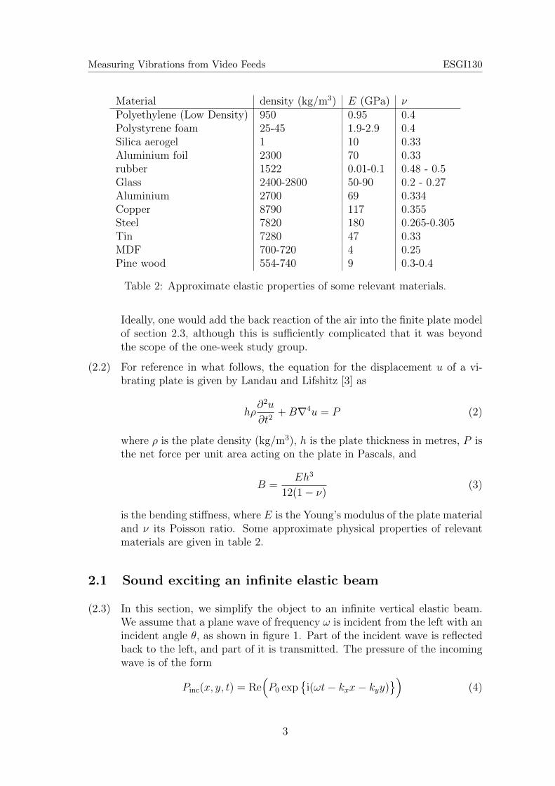
Material density (kg/m3) E (GPa) νPolyethylene (Low Density) 950 0.95 0.4Polystyrene foam 25-45 1.9-2.9 0.4Silica aerogel 1 10 0.33Aluminium foil 2300 70 0.33rubber 1522 0.01-0.1 0.48 - 0.5Glass 2400-2800 50-90 0.2 - 0.27Aluminium 2700 69 0.334Copper 8790 117 0.355Steel 7820 180 0.265-0.305Tin 7280 47 0.33MDF 700-720 4 0.25Pine wood 554-740 9 0.3-0.4

Table 2: Approximate elastic properties of some relevant materials.

Ideally, one would add the back reaction of the air into the finite plate modelof section 2.3, although this is sufficiently complicated that it was beyondthe scope of the one-week study group.

(2.2) For reference in what follows, the equation for the displacement u of a vi-brating plate is given by Landau and Lifshitz [3] as

hρ∂2u

∂t2+B∇4u = P (2)

where ρ is the plate density (kg/m3), h is the plate thickness in metres, P isthe net force per unit area acting on the plate in Pascals, and

B =Eh3

12(1− ν)(3)

is the bending stiffness, where E is the Young’s modulus of the plate materialand ν its Poisson ratio. Some approximate physical properties of relevantmaterials are given in table 2.

2.1 Sound exciting an infinite elastic beam

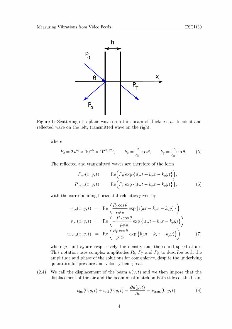
(2.3) In this section, we simplify the object to an infinite vertical elastic beam.We assume that a plane wave of frequency ω is incident from the left with anincident angle θ, as shown in figure 1. Part of the incident wave is reflectedback to the left, and part of it is transmitted. The pressure of the incomingwave is of the form

Pinc(x, y, t) = Re(P0 exp

{i(ωt− kxx− kyy)

})(4)

3


h

P

P

PT

R

0

xθ

Figure 1: Scattering of a plane wave on a thin beam of thickness h. Incident andreflected wave on the left, transmitted wave on the right.

where

P0 = 2√

2× 10−5 × 10dB/20, kx =ω

c0cos θ, ky =

ω

c0sin θ. (5)

The reflected and transmitted waves are therefore of the form

Pref(x, y, t) = Re(PR exp

{i(ωt+ kxx− kyy)

}),

Ptrans(x, y, t) = Re(PT exp


}), (6)

with the corresponding horizontal velocities given by

vinc(x, y, t) = Re

(P0 cos θ

ρ0c0exp


})vref(x, y, t) = Re

(−PR cos θ

ρ0c0exp

{i(ωt+ kxx− kyy)

})vtrans(x, y, t) = Re

(PT cos θ

ρ0c0exp


})(7)

where ρ0 and c0 are respectively the density and the sound speed of air.This notation uses complex amplitudes P0, PT and PR to describe both theamplitude and phase of the solutions for convenience, despite the underlyingquantities for pressure and velocity being real.

(2.4) We call the displacement of the beam u(y, t) and we then impose that thedisplacement of the air and the beam must match on both sides of the beam

vinc(0, y, t) + vref(0, y, t) =∂u(y, t)

∂t= vtrans(0, y, t) (8)

4


This implies that u(y, t) = Re(U exp

{i(ωt− kyy)

}), with

(P0 − PR) cos θ = iωρ0c0U = PT cos θ (9)

Equation (2) gives Newton’s law of motion applied to the beam,

hρ∂2u

∂t2+B

∂4u

∂y4= Pinc + Pref − Ptrans. (10)

Balancing the forces on the beam using (10) means that U must also satisfy(− ω2hρ+Bk4y

)U = P0 + PR − PT . (11)

Solving (9) and (11) simultaneously leads to

PT =iρ0c0ω

cos θU PR = P0 −

iρ0c0ω

cos θU (12)

U =2P0

Bω4

c40sin4θ − ω2hρ+ iω 2ρ0c0

cos θ

. (13)

Equation (13) therefore gives the amplitude and phase of the oscillation ofthe beam, subjected to an incoming wave of amplitude P0. Ideally, therefore,we would like the amplitude |U | to be as large as possible to be most easilydetected.

(2.5) Since (13) is relatively complicated, it is helpful to look at some simplifyingcases. In particular, for a wave perpendicular to the beam (sin θ = 0) thebending stiffness of the beam is unimportant, and we have

U =2P0

−ω2hρ+ 2iωρ0c0. (14)

In the limit of a very thin beam, or a very light beam, then hρ → 0, andwe recover |U | = |P0|/(ωρ0c0), which is the expression for the displacementof the air; that is, a light beam moves with the air. For a heavier or thickerbeam, the motion is smaller, especially at higher frequencies. The order ofmagnitude of the frequency when the beam stops moving with the air is givenby fc = 2πωc ∼ 4πρ0c0/(hρ). For frequencies much lower than this criticalfrequency fc the beam moves with the air, while for frequencies much higherthan fc the beam moves much less than the air.

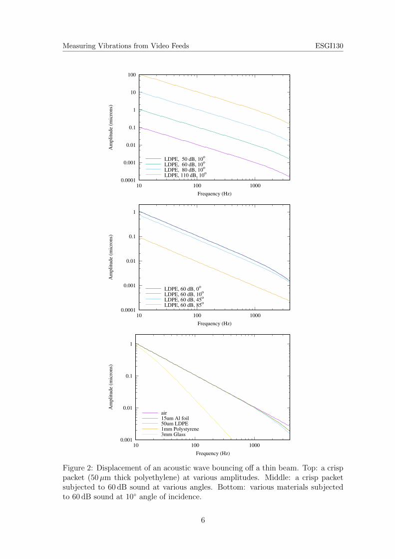
(2.6) Figure 2 plots the amplitude of oscillation |U | of various beams. The firsttwo sub-figures are for 50µm thick polyethylene, emulating a crisp packet.Louder amplitudes of sound lead to larger displacements, and higher frequen-cies lead to smaller displacements; this is expected, as a sound wave in airhas the same displacement profile. The displacement is relatively insensitiveto the direction of the incident sound, provided it is not parallel to the sur-face (θ = 90◦). The final sub-figure in figure 2 shows that several materials

5


0.0001

0.001

0.01

0.1

1

10

100

10 100 1000

Am

pli

tud

e (m

icro

ns)

Frequency (Hz)

LDPE, 50 dB, 10o

LDPE, 60 dB, 10o

LDPE, 80 dB, 10o

LDPE, 110 dB, 10o

0.0001

0.001

0.01

0.1

1

10 100 1000

Am

pli

tud

e (m

icro

ns)

Frequency (Hz)

LDPE, 60 dB, 0o

LDPE, 60 dB, 10o

LDPE, 60 dB, 45o

LDPE, 60 dB, 85o

0.001

0.01

0.1

1

10 100 1000

Am

pli

tud

e (m

icro

ns)

Frequency (Hz)

air15um Al foil50um LDPE1mm Polystyrene3mm Glass

Figure 2: Displacement of an acoustic wave bouncing off a thin beam. Top: a crisppacket (50µm thick polyethylene) at various amplitudes. Middle: a crisp packetsubjected to 60 dB sound at various angles. Bottom: various materials subjectedto 60 dB sound at 10◦ angle of incidence.

6


act the same, and effectively just act as passive tracers of the vibration inthe air, at least at low to moderate frequencies, while high frequencies aremore attenuated. This is not the case for all materials, however; 3 mm thickglass has a much smaller amplitude, especially at higher frequencies.

(2.7) This model is of course a rather simple one. For example, it assumes thatthe object is an infinite flat beam with no curvature or edges, that the beamis not clamped or pinned in any way, and that the incoming wave is onlypresent to the left of the beam. Some of these could be incorporated asextensions of this model. This model also ignores resonances as is assumesan infinite beam. Resonant frequencies occur in all finite elastic scatterers,causing the acoustic displacement to be much greater than at other non-resonant frequencies. In order to investigate resonance, we next describe amodel of a finite size elastic plate and its resonances.

2.2 Resonances of a 2D rectangular plate

(2.8) In this section, we develop a model of the resonances of an elastic platesupported by its edges. We assume a rectangular plate of size Lx × Lyresting on its edges and solve the unforced 2D version of (2),

hρ∂2u

∂t2+B∇4u = 0. (15)

We use separation of variables and take u(t, x, y) = g(t)W (x, y). Then

hρ

g

∂2g

∂t2= − B

W

(∂4W

∂x4+∂4W

∂y4+ 2

∂4W

∂x2∂y2

). (16)

For equality to hold, both sides must be a constant, say −ω2, and we maytherefore take g(t) = sin(ωt). Then

B

ρh

(∂4W

∂x4+∂4W

∂y4+ 2

∂4W

∂x2∂y2

)= ω2W. (17)

We then impose the boundary conditions for a freely supported resting platewith no bending moments at the edges:

W (0, y) = W (Lx, y) = W (x, 0) = W (x, Ly) = 0 (18)

B

(∂2W

∂x2+ ν

∂2W

∂y2

)= 0, at x = 0 and x = Lx (19)

B

(∂2W

∂y2+ ν

∂2W

∂x2

)= 0, at y = 0 and y = Lx. (20)

We then notice that W (x, y) = A sin(kxx) sin(kyy) satisfies trivially all theabove boundary conditions if kx = nπ/Lx and ky = mπ/Ly where n and m

7


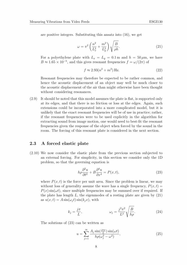
are positive integers. Substituting this ansatz into (16), we get

ω = π2

(n2

L2x

+m2

L2y

)√B

ρh. (21)

For a polyethylene plate with Lx = Ly = 0.1 m and h = 50µm, we haveB ≈ 1.65× 10−5, and this gives resonant frequencies f = ω/(2π) of

f ≈ 2.93(n2 +m2) Hz. (22)

Resonant frequencies may therefore be expected to be rather common, andhence the acoustic displacement of an object may well be much closer tothe acoustic displacement of the air than might otherwise have been thoughtwithout considering resonances.

(2.9) It should be noted that this model assumes the plate is flat, is supported onlyat its edges, and that there is no friction or loss at the edges. Again, suchextensions could be incorporated into a more complicated model, but it isunlikely that the exact resonant frequencies will be of use in practice; rather,if the resonant frequencies were to be used explicitly in the algorithm forextracting sound from image motion, one would need to best-fit the resonantfrequencies given the response of the object when forced by the sound in theroom. The forcing of this resonant plate is considered in the next section.

2.3 A forced elastic plate

(2.10) We now consider the elastic plate from the previous section subjected toan external forcing. For simplicity, in this section we consider only the 1Dproblem, so that the governing equation is

hρ∂2u

∂t2+B

∂4u

∂x4= P (x, t), (23)

where P (x, t) is the force per unit area. Since the problem is linear, we maywithout loss of generality assume the wave has a single frequency, P (x, t) =P (x) sin(ωt), since multiple frequencies may be summed over if required. Ifthe plate has length L, the eigenmodes of a resting plate are given by (21)as u(x, t) = A sin(ωjt) sin(kjx), with

kj =jπ

L, ωj =

j2π2

L2

√B

hρ. (24)

The solutions of (23) can be written as

u =∞∑j=1

Aj sin( jπxL

) sin(ωt)

hρ(ω2j − ω2)

, (25)

8


10 100 1000Frequency (Hz)

10 1

101

103

105

107

Amplitude (m

icron)

N=60dBN=80dBN=100dBN=120dB

10 100 1000Frequency (H )

10−1

100

101

102

103

104

105

106

107

Amplitu

de (m

icron

)

N=60dBN=80dBN=100dBN=120dB

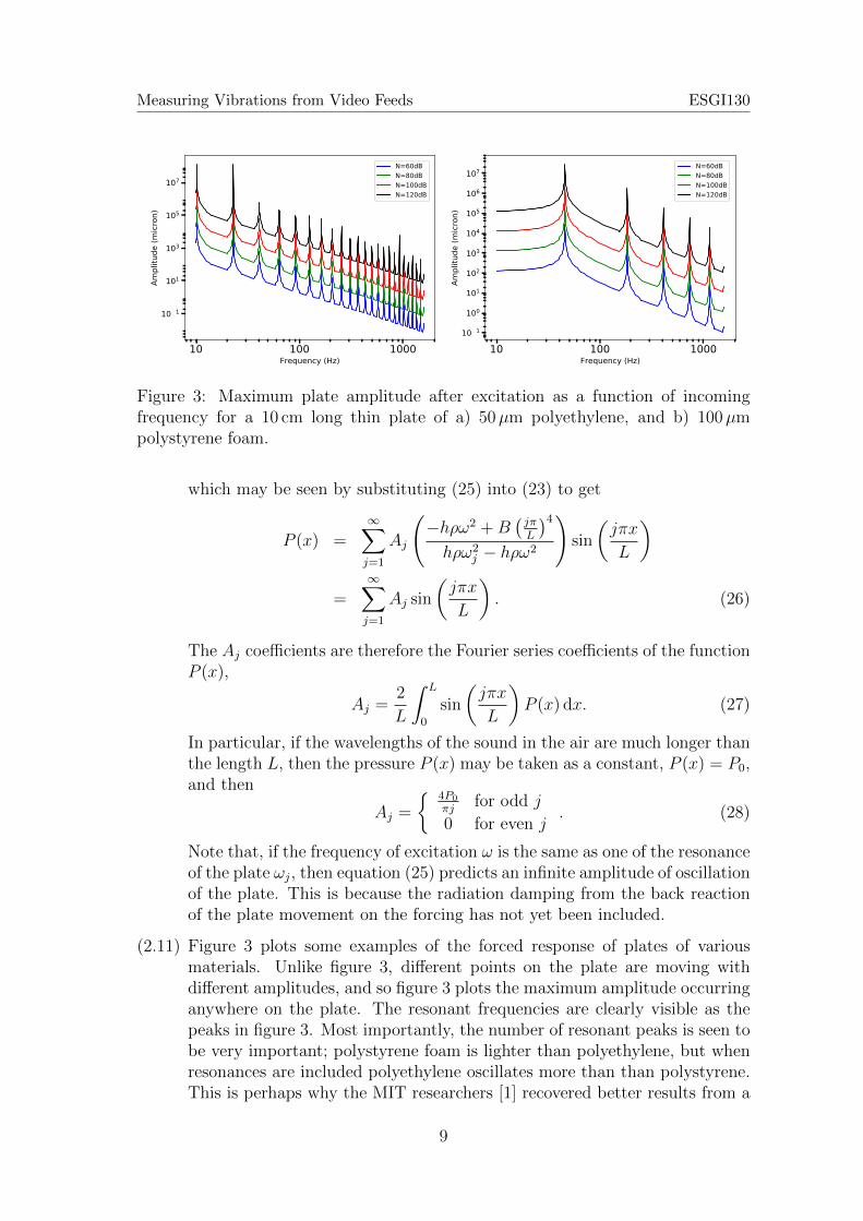
Figure 3: Maximum plate amplitude after excitation as a function of incomingfrequency for a 10 cm long thin plate of a) 50µm polyethylene, and b) 100µmpolystyrene foam.

which may be seen by substituting (25) into (23) to get

P (x) =∞∑j=1

Aj

(−hρω2 +B

(jπL

)4hρω2

j − hρω2

)sin

(jπx

L

)

=∞∑j=1

Aj sin

(jπx

L

). (26)

The Aj coefficients are therefore the Fourier series coefficients of the functionP (x),

Aj =2

L

∫ L

0

sin

(jπx

L

)P (x) dx. (27)

In particular, if the wavelengths of the sound in the air are much longer thanthe length L, then the pressure P (x) may be taken as a constant, P (x) = P0,and then

Aj =

{4P0

πjfor odd j

0 for even j. (28)

Note that, if the frequency of excitation ω is the same as one of the resonanceof the plate ωj, then equation (25) predicts an infinite amplitude of oscillationof the plate. This is because the radiation damping from the back reactionof the plate movement on the forcing has not yet been included.

(2.11) Figure 3 plots some examples of the forced response of plates of variousmaterials. Unlike figure 3, different points on the plate are moving withdifferent amplitudes, and so figure 3 plots the maximum amplitude occurringanywhere on the plate. The resonant frequencies are clearly visible as thepeaks in figure 3. Most importantly, the number of resonant peaks is seen tobe very important; polystyrene foam is lighter than polyethylene, but whenresonances are included polyethylene oscillates more than than polystyrene.This is perhaps why the MIT researchers [1] recovered better results from a

9


crisp packet (made of polyethylene) than they did from a disposable drinkscup (made of polystyrene foam). Note that the amplitudes of oscillation infigure 3 are larger than those in figure 2, since in figure 2 energy is lost byradiating sound back into the air.

(2.12) In this section, we have neglected any dissipation that might limit resonance,such as dissipation within the air or friction of the plate with its supports.The forcing was also considered given and the response of the plate wascalculated; this neglects the back reaction of the plate movement on thewave in the air, which will also limit the amplitude at resonance. This isaddressed in the next section.

2.4 Interaction between sound and a resonating object

(2.13) In the analysis above, section 2.1 accounts for the back reaction of the plateon the air (through wave reflection and transmission), but ignores resonances.Contrastingly, section 2.3 includes resonances, but ignores the back reactionof the plate on the air, leading to arbitrarily large plate motion at the res-onant frequencies. In this section, we modify the model in section 2.1 toinclude an artificial spring and damping term, in order to investigate thecombination of back reaction and resonance.

(2.14) We modify Newton’s law for the beam (10) to include an artificial springterm hρω2

0 (giving an undamped resonance at frequency ω0) and an artificialdamping µ. One could think of this as a crude model of a horizontal beamlying on a carpet, with the carpet providing the extra spring and damp-ing terms, and the transmitted wave being totally absorbed by the carpetwithout reflection. The resulting governing equation is

hρ∂2u

∂t2+ µ

∂u

∂t+ hρω2

0u+B∂4u

∂y4= Pinc + Pref − Ptrans. (29)

By following the same method as in section 2.1, we arrive at the equivalentof equation (13),

U =2P0

Bω4

c40sin4θ + (ω2

0 − ω2)hρ+ iω(µ+ 2ρ0c0

cos θ

) , (30)

or, for a wave perpendicular to the beam (sin θ = 0), the equivalent ofequation (14),

U =2P0

(ω20 − ω2)hρ+ iω(µ+ 2ρ0c0)

. (31)

This shows that the 2iωρ0c0 term found previously is a radiation dampingterm, which is increased by adding the artificial damping µ, while the reso-nance at ω0 can cancel out the mass of the beam so as to give results nearresonance as if the beam were much lighter. Without artificial damping

10


0.001

0.01

0.1

1

10 100 1000

Am

pli

tude

(mic

rons)

Frequency (Hz)

AirGlassGlass + ResonanceGlass + Resonance + DampingGlass + Resonance (Fixed Forcing)

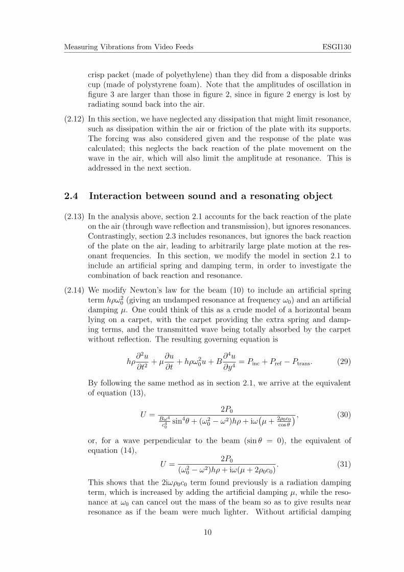
Figure 4: Amplitude of oscillations of a beam with an artificial spring (resonantfrequency ω0) and damping (strength µ), using (31). Air is the displacement of theair for the incoming wave. Glass is for 3 mm thick glass. Glass+Resonance is forglass with an artificial spring resonating at 100 Hz. Glass+Resonance+Dampingadds an additional damping of strength µ = 2ρ0c0 (comparable to the radiationdamping). “Fixed forcing” assumes no back reaction of the beam on the air (as insection 2.3).

(µ = 0), at resonance we recover U = P0/(iωρ0c0), which is the displacementamplitude of the air. Without both artificial and radiation damping (settingµ = ρ0 = 0), we find an infinite beam amplitude at resonance when ω = ω0,in agreement with the results of the previous section.

(2.15) Figure 4 plots the results of this for a 3 mm thick glass beam. With anartificial resonance at 100 Hz, the amplitude of oscillation of the beam at100 Hz is the same as that of the air, while without the artificial resonancethe beam amplitude is ten times smaller. Adding extra dissipation reducesthe amplitude at resonance, while ignoring the radiation damping (by usinga fixed forcing as in section 2.3) gives the expected infinite amplitude atresonance.

(2.16) Importantly, note that introducing a resonance can also have negative effects,such as anti-resonance. This can be seen at low frequencies in figure 4,where the amplitude of the glass with artificial resonance is much smallerthan the amplitude of the glass without artificial resonance. As is knownfrom current research on generating electricity from water waves, designingresonant systems to capture energy from waves is far from easy.

11


Mirror

Mirror’

d

Object

Image

Image’

Observer

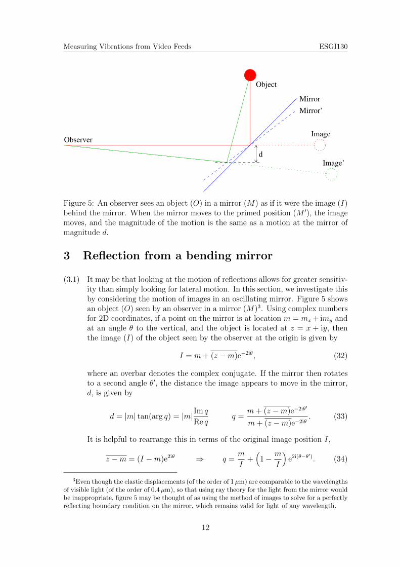
Figure 5: An observer sees an object (O) in a mirror (M) as if it were the image (I)behind the mirror. When the mirror moves to the primed position (M ′), the imagemoves, and the magnitude of the motion is the same as a motion at the mirror ofmagnitude d.

3 Reflection from a bending mirror

(3.1) It may be that looking at the motion of reflections allows for greater sensitiv-ity than simply looking for lateral motion. In this section, we investigate thisby considering the motion of images in an oscillating mirror. Figure 5 showsan object (O) seen by an observer in a mirror (M)3. Using complex numbersfor 2D coordinates, if a point on the mirror is at location m = mx + imy andat an angle θ to the vertical, and the object is located at z = x + iy, thenthe image (I) of the object seen by the observer at the origin is given by

I = m+ (z −m)e−2iθ, (32)

where an overbar denotes the complex conjugate. If the mirror then rotatesto a second angle θ′, the distance the image appears to move in the mirror,d, is given by

d = |m| tan(arg q) = |m|Im q

Re qq =

m+ (z −m)e−2iθ′

m+ (z −m)e−2iθ. (33)

It is helpful to rearrange this in terms of the original image position I,

z −m = (I −m)e2iθ ⇒ q =m

I+(

1− m

I

)e2i(θ−θ

′). (34)

3Even though the elastic displacements (of the order of 1µm) are comparable to the wavelengthsof visible light (of the order of 0.4µm), so that using ray theory for the light from the mirror wouldbe inappropriate, figure 5 may be thought of as using the method of images to solve for a perfectlyreflecting boundary condition on the mirror, which remains valid for light of any wavelength.

12


m/I is the distance to the mirror normalized by the distance to the image.Since the image is always “behind” the mirror, this ratio always has modulusless than one. If the image is a significant distance away, such as the reflectionof the sun, moon, or clouds, then |m/I| � 1, and in this case for smallangular changes θ − θ′, we find |d| = 2|m||θ − θ′|. This is to be expected;if you were looking at yourself in a hand mirror, and then turned the handmirror 45◦ upwards, you would see the ceiling in the mirror, which is a90◦ = 2× 45◦ change in direction.

(3.2) How does this compare with the motion of an actual object? For example, arewe better to look at the motion of a crisp packet, or the motion of reflectionsin the crisp packet? In order to answer this, we consider a mirrored bendingbeam. The bottom of the beam is fixed, while the top of the beam hasmoved a distance a. The shape of the beam is therefore given by x = ay2/`2,where ` is the length of the beam. The angle of the top of the beam, forsmall deflections, is approximately θ′ ≈ dx

dy|y=` = 2a/`, and therefore the

displacement of a reflection in the top of the beam is d ≈ 4|m|a/`; that is, thedisplacement a is magnified by a factor 4|m|/` when looking at the reflection,where ` is the length of the beam (e.g. the size of the object) and |m| isthe distance to the camera. Clearly |m| � `, and hence tracking movingreflections in objects is predicted to lead to significantly better sensitivitythan just tracking lateral motion of the object. As an example, for an objectof size ` = 10 cm oscillating with 1µm amplitude viewed from a camera|m| = 10 m away, the effective motion of reflections in the object is predictedto be of the order d = 400µm, which should easily be detectable.

(3.3) This section assumes that there are suitable objects in a room to causereflections (such as lights, windows, etc), and that motion of reflections maybe detected as easily as motion of the object itself. This latter assumptionis probably quite limiting, since diffusive reflections may be much harder toget accurate motion from. Practical tests with oscillating reflective objectswould be helpful to test the validity of these assumptions.

4 Detecting motion from video

(4.1) The underlying process behind the visual microphone MIT paper [1] relieson being able to amplify the motion of object in a video at certain frequen-cies; this is described by a previous publication by MIT researchers Wadhwaet al. [7]. The process makes use of a “complex-valued steerable pyramid”wavelet decomposition [4–6]. As described by [5], the is overcomplete (i.e.produces more bytes of data than the input), but is invertible (so that theoriginal image can be reconstructed from the wavelet coefficients). The sig-nal is separated into high-, low-, and band-limited spatial frequencies. Thehigh-frequencies are stored unencoded. The band-limited frequencies are

13


encoded using several different positions and orientations of wavelets. Thelow-frequencies are downsampled to half the resolution, and the process re-peated (hence the pyramid structure). This ensures details of the image atseveral different scales and at several different orientations is produces.

(4.2) Just as for a Fourier series, Wadhwa et al. [7] claim that the complex coeffi-cients of the resulting transform can be separated into their amplitude andphase, with a change in phase corresponding to translation. By transformingeach frame of a video, the phase of each coefficient can have particular tem-poral frequencies amplified, which then amplifies the motion in the image atthese frequencies. The same technique of using the phase of each coefficientwas used for the visual microphone paper by Davis et al. [1].

(4.3) Because of the pyramid structure of the wavelets, information about the mo-tion of the entire image will be encoded using the coefficients at the bottomof the pyramid. While these coefficients were not treated differently than theother coefficients in the MIT papers, it is likely that using these coefficientscarefully could eliminate camera movements from the signal; although thiswas not investigated further here.

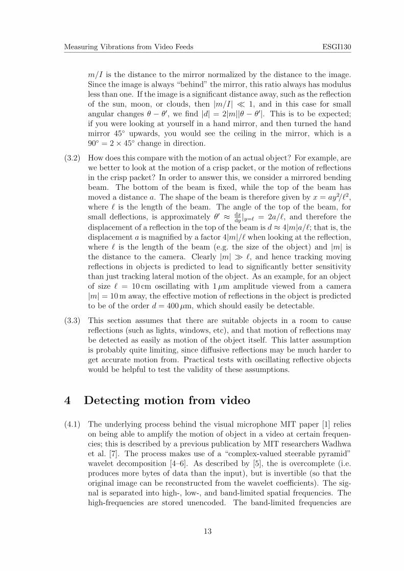
(4.4) To investigate the detection of motion from videos, we take the code fromRef. 7, available online4, and investigate some of the results from the paper,and our own example. For our own example, we excite a projector screen ofapproximate height h = 3.5m, and film the oscillations with both a DSLRcamera on a tripod and a hand-held mobile phone camera. The frame ratefor both was 30fps, with a video size of 960× 480 pixels. We take advantageof the first few resonant frequencies of the screen. Treating the screen as asimple pendulum gives an (angular) frequency of

√h/g, while adding in some

effects of torsion instead gives√

3h/g as the angular frequency. Convertingto Hz then gives frequencies in the range 0.26-0.46Hz. We therefore chooseto selectively amplify from 0.2Hz to 0.6Hz when using the MIT software.The running time on a standard laptop were on the order of several minutes,depending on the video length and number of frames; our processing used areduced resolution video to speed up the computation, as can be seen in thefigures below when comparing the original and motion enhanced images.

(4.5) We get good results for both the mobile phone footage and DSLR footage,provided the cameras are held steady. We recover the oscillations of theprojector at the expected frequencies. Some stills from these movies aredisplayed in Figure 6.

(4.6) We are able to detect and magnify the motion, even when the video framerate is reduced to 2fps. We do this by just selected the 15-th and 30-th frameper second.

4http://people.csail.mit.edu/nwadhwa/phase-video/PhaseBasedRelease_20131023.

zip

14

http://people.csail.mit.edu/nwadhwa/phase-video/PhaseBasedRelease_20131023.zip

http://people.csail.mit.edu/nwadhwa/phase-video/PhaseBasedRelease_20131023.zip


(a) Original image (b) Motion magnified image

Figure 6: Stills from the unmagnified (left) and motion magnified (right) videos ofa moving projector screen. Note that, to save processing time, the quality of thevideo on the right has been reduced.

(4.7) We are able to add noise to the original video of a crane that appears tobe stationary, and still detect the motion of the crane at 0.2Hz to 0.4Hz asdiscussed in Wadhwa et al. [7]. It was pointed out in Wadhwa et al. [7] thatthis is entirely expected, since the technique may redistribute noise but willnever amplify it. The noise we added was Gaussian white noise with zeromean and variance σ2 = 0.01, using the “imnoise” command in Matlab.

(4.8) If the camera is moving (such as a hand held mobile phone footage), we areunable to get sensible results due to the motion of the camera. We see thewhole image moving, and it is difficult to detect what is still and what is notafter applying the algorithm. Pre processing to reduce the movement of thecamera might improve the algorithm, but it was not tested here.

(4.9) We conclude that the software is working reasonably well and able to be usedon a standard laptop. Using larger image sizes requires more memory, whichwas the main limiting factor in the image size we choose.

4.1 Rolling shutter

(4.10) We now investigate the effect of a rolling shutter, which allows the recoveryof higher frequencies that the frame rate. This technique was suggested inDavis et al. [1].

(4.11) For example, let us consider the case of a 50fps standard camera, and wantedto detect motion at 200Hz, i.e four times faster than the frame rate. Forsimplicity, we assume we have a couple of objects which move from position1 to position 2 at a frequency of 200Hz.

(4.12) If we have a global shutter, then we capture all the information in the imageat one moment. Thus, we would only see the image at position 1 if wecapture the image using the global shutter.

(4.13) If we instead have a rolling shutter, then each line is exposed for a smallamount of time (with a typical minimum exposure time of 1/2000s, so in

15


Position 1

Position 2

1000 lines

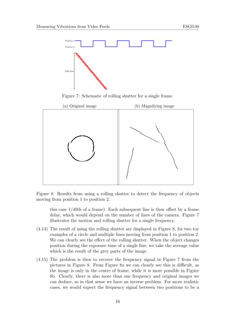
Figure 7: Schematic of rolling shutter for a single frame.

(a) Original image (b) Magnifying image

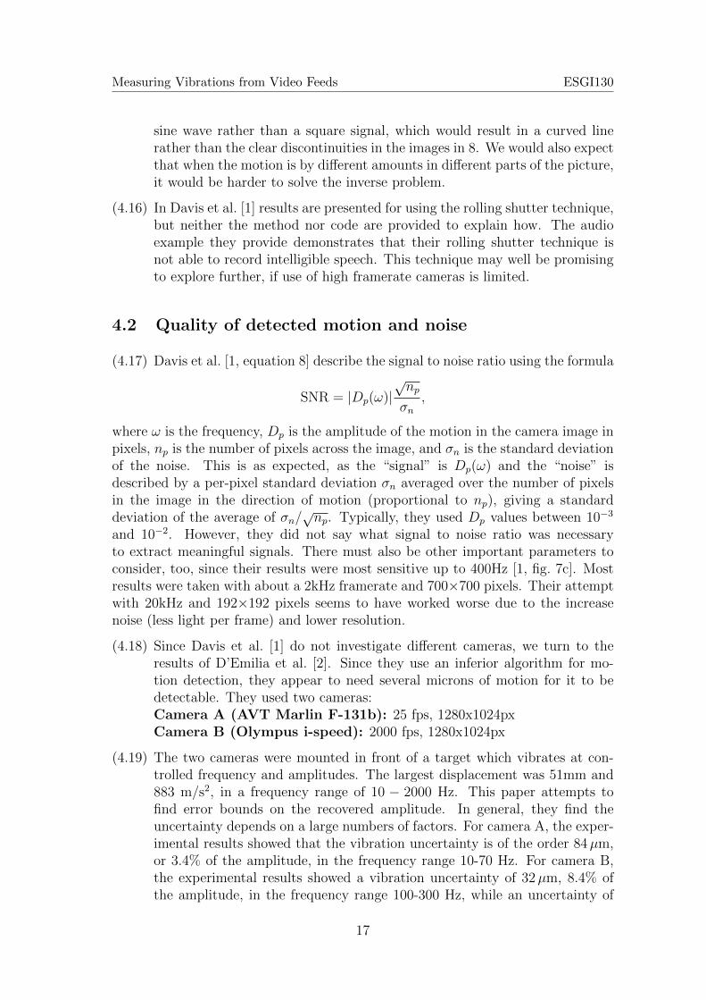
Figure 8: Results from using a rolling shutter to detect the frequency of objectsmoving from position 1 to position 2.

this case 1/40th of a frame). Each subsequent line is then offset by a framedelay, which would depend on the number of lines of the camera. Figure 7illustrates the motion and rolling shutter for a single frequency.

(4.14) The result of using the rolling shutter are displayed in Figure 8, for two toyexamples of a circle and multiple lines moving from position 1 to position 2.We can clearly see the effect of the rolling shutter. When the object changesposition during the exposure time of a single line, we take the average valuewhich is the result of the grey parts of the image.

(4.15) The problem is then to recover the frequency signal in Figure 7 from thepictures in Figure 8. From Figure 8a we can clearly see this is difficult, asthe image is only in the centre of frame, while it is more possible in Figure8b. Clearly, there is also more than one frequency and original images wecan deduce, so in that sense we have an inverse problem. For more realisticcases, we would expect the frequency signal between two positions to be a

16


sine wave rather than a square signal, which would result in a curved linerather than the clear discontinuities in the images in 8. We would also expectthat when the motion is by different amounts in different parts of the picture,it would be harder to solve the inverse problem.

(4.16) In Davis et al. [1] results are presented for using the rolling shutter technique,but neither the method nor code are provided to explain how. The audioexample they provide demonstrates that their rolling shutter technique isnot able to record intelligible speech. This technique may well be promisingto explore further, if use of high framerate cameras is limited.

4.2 Quality of detected motion and noise

(4.17) Davis et al. [1, equation 8] describe the signal to noise ratio using the formula

SNR = |Dp(ω)|√np

σn,

where ω is the frequency, Dp is the amplitude of the motion in the camera image inpixels, np is the number of pixels across the image, and σn is the standard deviationof the noise. This is as expected, as the “signal” is Dp(ω) and the “noise” isdescribed by a per-pixel standard deviation σn averaged over the number of pixelsin the image in the direction of motion (proportional to np), giving a standarddeviation of the average of σn/

√np. Typically, they used Dp values between 10−3

and 10−2. However, they did not say what signal to noise ratio was necessaryto extract meaningful signals. There must also be other important parameters toconsider, too, since their results were most sensitive up to 400Hz [1, fig. 7c]. Mostresults were taken with about a 2kHz framerate and 700×700 pixels. Their attemptwith 20kHz and 192×192 pixels seems to have worked worse due to the increasenoise (less light per frame) and lower resolution.

(4.18) Since Davis et al. [1] do not investigate different cameras, we turn to theresults of D’Emilia et al. [2]. Since they use an inferior algorithm for mo-tion detection, they appear to need several microns of motion for it to bedetectable. They used two cameras:Camera A (AVT Marlin F-131b): 25 fps, 1280x1024pxCamera B (Olympus i-speed): 2000 fps, 1280x1024px

(4.19) The two cameras were mounted in front of a target which vibrates at con-trolled frequency and amplitudes. The largest displacement was 51mm and883 m/s2, in a frequency range of 10 − 2000 Hz. This paper attempts tofind error bounds on the recovered amplitude. In general, they find theuncertainty depends on a large numbers of factors. For camera A, the exper-imental results showed that the vibration uncertainty is of the order 84µm,or 3.4% of the amplitude, in the frequency range 10-70 Hz. For camera B,the experimental results showed a vibration uncertainty of 32µm, 8.4% ofthe amplitude, in the frequency range 100-300 Hz, while an uncertainty of

17


13µm could be achieved (13% of vibration amplitude) in the range 400-600Hz. In the paper, camera B had an error bound much greater than 10%when considering a low contrast object, for frequencies 300,400 & 500 Hz.Consequently the authors did not analyse this. This could hint at possibleproblems when analysing video. The paper does not consider object illumi-nation, which could be a large cause of uncertainty for everyday applications.

(4.20) It is unclear how these results should be applied to the MIT technique [1],although it is clear that the detectable signal depends strongly on the charac-teristics of the camera used. We would therefore propose further experimentsusing high-speed cameras to investigate the dependence of motion detectionon important factors such as the amount of ambient light and the clarityof the image. We propose a thin sheet or strip of some suitable material(such as LDPE) be held vertically, with the top able to be excited horizon-tally (for example by connecting it to a horizontal loud speaker) and thebottom allowed to move freely, possibly with some added weight at bottom.A high-speed camera would video the motion of the sheet from the side, sothat the sheet would appear as a line oscillating left-right in the video. TheMIT software would then be used to extract the motion of the sheet from thevideo. Direct measurements of the oscillation of the sheet could also be madeby other means for comparison. Experiments could then be conducted withdifferent cameras, different framerates, different lighting conditions, differentcamera lenses and distances, and different amplitudes of oscillation, to mapout the conditions necessary for successfully detecting motion, and the corre-sponding noise. This setup could be used with a second loud speaker in theair, allowing the analysis of section 2 to be validated. Moreover, this setupcould also be used to investigate the use of rolling shutters (see section 4.1),since each horizontal line of the video will see a slightly different part of thesheet at a slightly different time; this would be particularly interesting whenthe frame rate of the camera is lower than the natural period of the sheet.

5 Intelligible speech

(5.1) As described in the introduction, voices consist of frequencies from around80Hz to around 4kHz. Telephone systems use the range 300Hz to 3.4kHz forspeech. From their figures, Davis et al. [1] claim to recover intelligible speechusing what appears to be only the 250Hz to 850Hz range. In this section,we investigate the requirements for intelligible speech with a focus on thisrange.

(5.2) This study used list 5 of the “Harvard sentences”5, which are short sentenceseach containing 5 important words to be identified. The sentences used were:

5http://www.cs.columbia.edu/~hgs/audio/harvard.html

18

http://www.cs.columbia.edu/~hgs/audio/harvard.html


700 800 900 1000 1100 1200 4000

Max frequency (Hz)

0.01

0.02

0.05

0.080.1

0.2

0.3

0.5

Nois

e le

vel

44%

45%

40%

44%

15%

13%

88%

55%

33%

60%60%

80%80%

30%40% 76%

0%

5%

0%

46%

40%

40%

46%

15%

28%

Figure 9: Plot of the average intelligibility (on a percentage scale, with 100% beingfully intelligible) of sample sentences with a given lowpass frequency and a givennoise level. Based on a very small study of 108 sentences.

1. A king ruled the state in the early days.

2. The ship was torn apart on the sharp reef.

3. Sickness kept him home the third week.

4. The wide road shimmered in the hot sun.

5. The lazy cow lay in the cool grass.

6. Lift the square stone over the fence.

7. The rope will bind the seven books at once.

8. Hop over the fence and plunge in.

9. The friendly gang left the drug store.

Recordings of these sentences were then bandpassed, and white noise added. Theupper limit of the bandpass and the amplitude of the noise was varied, with the lowerlimit of the bandpass set to 300 Hz. In total 12 people each listened to 9 sentencesand attempted to identify the 5 important words, leading to an intelligibility scorebetween 0 and 5. The results are summarized in figure 9.

It is clear that a larger sample is needed to get a well-converged average. However, itis also clear that there is a large amount of random variation, with the bottom rightcorner of figure 9 suggesting that the highest 4kHz cutoff frequency and the lowestnoise was necessary to give a repeatably intelligible signal (this being comparableto telephony quality). Based on this, we suggest at a minimum aiming to capture300Hz to 1.2kHz for a reasonable chance at recognising speech. Not shown in this

19


figure, but notable from our study, was that native speakers were more able tocorrectly identify the speech against a noisy background than non-native speakers,even for those non-native speakers with otherwise excellent English.

The results of Davis et al. [1] available to listen to have very little noise, suggestingthey have been post-processed to aid intelligibility. Indeed, Davis et al. [1] refer to anumber of standard speech enhancement techniques which we have not investigatedfurther here. A description of a possible mathematical basis for enhanced speechrecovery using Bayesian inference is presented in appendix A.1.

6 Conclusion

(6.1) This project investigated the feasibility of using the MIT visual microphonetechnique [1] to recover intelligible speech from high speed video recordings.

(6.2) The MIT experiments [1] depended on loud sound and prior knowledge of“Mary had a little lamb”. Their equipment would not have recovered intel-ligible speech at conversational volume, or if what was being said was notknown beforehand.

(6.3) Object oscillations of the order of 0.1µm need to be detectable in order torecover speech at conversational volumes. The MIT technique is able toextract motion from videos that at least 1/1000th of a pixel, which givesan indication of the level of magnification of the image needed: at least 10pixels per millimeter, and preferably 100 pixels per millimeter.

(6.4) The investigation in section 5 suggests that, for intelligible speech, we wouldneed to capture at least up to 1.2 kHz, and preferrably higher (potentially3.4 kHz for telephony quality sound). The MIT technique is able to detectfrequencies up to about 850 Hz using a 2,200 fps camera, suggesting thatat least a 3,100 fps camera is needed, and potentially a 9,000 fps camera.However, when the MIT researchers tried higher framerates, they found theincreased noise made intelligibility harder. Clearly understatnding the signalto noise ratio of the captured sound is important.

(6.5) While we would have liked to be able to give explicit advice about the hard-ware requirements for obtaining intelligible speech using the MIT technique,to do so would need further experiments. The model of signal to noise ratioin the MIT paper [1] is experimentally derived, and does not account forchanges in ambient lighting or camera framerate, camera pixel noise (ISOsetting), image clarity (e.g. caused by imperfect camera lenses), nor does itdescribe the frequency dependence of the signal to noise ratio. A suggestionfor a possible future experiment is described at the end of section 4.2.

(6.6) Whatever the specific requirements, a high speed, low noise camera is essen-tial. Existing video footage is unlikely to be of sufficient quality or sufficientlyhigh frame rate.

20


(6.7) While MIT report using the rolling shutter of a camera to capture frequenciesmuch higher than the camera frame rate, this did not result in intelligiblespeech (or even in identifiable speech), and the MIT algorithm for doing thishas not been made public. While a much more complicated and challengingproblem, we see no fundamental reason why rolling shutters could not betaken advantage of if access to high speed cameras is limited.

(6.8) The MIT experiments depend on the motion of light objects (such as crisppackets or disposable cups), but resonances of heavier objects (e.g. curtains)could potentially also be exploited (section 2.4. Due to the drop in oscillatingamplitude with increasing frequency (figure 2), it is likely that only thefirst few resonances will be useful, which could simplify the task of takingadvantage of resonances; the MIT results are also suggestive that only thefirst few modes are important [1, figure 5]. The closer together the resonancesare, the larger the resulting motion (figure 3).

(6.9) By looking at reflections in objects, much more subtle motion could be de-tectable, possibly including speech at conversational volumes. For example,using reflections in a bending 10 cm mirror viewed from 10 m gives a 400×magnification of motion.

(6.10) Vibrations of the camera were ignored by MIT, but are expected to be sig-nificant. The MIT technique could probably be adapted to be resilient tocamera vibrations, by using the lowest resolution wavelets as a proxy forwhole-scene motion, although this was not attempted here.

(6.11) We are sceptical of the MIT claim that optimized computer code could pro-cess video in real time. The technique is highly parallelizable, however, socould possibly be offloaded to a supercomputer for real-time processing.

(6.12) The effect of video compression artifacts was not considered in this work, norby MIT. Modern video compression (such as H.264 and H.265 codecs oftenused in mp4 files) use motion estimation to enhance compression, and themotion estimation used is unlikely to be sufficiently accurate to recover thesubtle motions needed for the MIT technique.

(6.13) Also not considered here or by MIT is aliasing, where frequencies higher thanhalf the camera frame rate alias and become artifacts at lower frequencies.In audio recording, it is essential to use a low-pass filter before digitising thesound in order to eliminate aliasing, but this cannot be done with currenthigh-speed cameras.

(6.14) It may be possible to build cheap counter-measures to counter this technique.For example, small oscillators (such as the vibration units in mobile phones)could be stuck onto surfaces and generate small amounts of white noiseoscillations. These would be inaudible to people in the room, but wouldrender the visual microphone technique impossible.

21


A Appendices

A.1 Recognising speech from a noisy background

(A.1.1) Inferring speech from the minuscule vibrations in video would be enhancedif one had a strong prior probability distribution on speech. Singing is welldescribed as filtered white noise. Perhaps speech could be too. The filteris a function of time, to make the changes in phonemes, pitch, loudness,speaker etc. One could model this by a Markov process.

(A.1.2) Suppose the sound source x is given by

x = Gx+ Lu (35)

where G is an asymptotically stable linear map, u is a vector of unit whitenoises, and L is a linear map.

(A.1.3) Model the response y of the objects in the sound field as a linear system

y = Fy +Mx+ Pv (36)

where F is another asymptotically stable linear map, M a linear map, vsome more white noises, and P a linear map.

(A.1.4) Model the observations z by

z = Kz +Hy +Nw (37)

with K asymptotically stable, H,N linear, and w more white noises. Onecould take z to be an instantaneous measurement, e.g. z = −K−1Hx + εas would result from K being large, but in general one might expect somecorrelations between the measurement errors ε and the above formulationgives some.

(A.1.5) Then the full system is xyz

=

G 0 0M F 00 H K

xyz

+

L 0 00 P 00 0 N

uvw

. (38)

The problem is to infer the function x from the function z. This is aKalman filter problem and has a standard efficient solution. The matricesare unknown, however, so they would also need to be inferred. There issome redundancy in the description, e.g. for the matrix, call it C, in frontof the white noises, only the matrix CCT matters, and one could applylinear coordinate changes to x and y, so before attempting to infer thematrices it might be best to normalise them. Furthermore, it is likely

22


that only the lightest damped modes of F matter, so one could attempt ahighly reduced description of F .

(A.1.6) Extension to allow the filter G and noise amplitudes L to vary slowly intime takes one out of the autonomous regime for the efficient Kalman filtersolution, but it is still a Gaussian process so may be relatively feasible todo the inference.

References

[1] Davis, A., M. Rubinstein, N. Wadhwa, G. Mysore, F. Durand, and W. T. Free-man (2014). The visual microphone: Passive recovery of sound from video. ACMTransactions on Graphics (Proc. SIGGRAPH) 33 (4), 79:1–79:10.

[2] D’Emilia, G., L. Razze, and E. Zappa (2013). Uncertainty analysis of highfrequency image-based vibration measurements. Measurement 46 (8), 2630–2637.

[3] Landau, L. D. and E. Lifshitz (1970). Theory of Elasticity (2nd ed.). Pergamon.

[4] Portilla, J. and E. P. Simoncelli (2000). A parametric texture model based onjoint statistics of complex wavelet coefficients. Int. J. Comp. Vis. 40 (1), 49–71.

[5] Simoncelli, E. P. and W. T. Freeman (1995). The steerable pyramid: A flexiblearchitecture for multi-scale derivative computation. In Proc. 2nd IEEE Interna-tional Conference on Image Processing, Washington DC, Volume 3, pp. 444–447.

[6] Simoncelli, E. P., W. T. Freeman, E. H. Adelson, and D. J. Heeger (1992).Shiftable multi-scale transforms. IEEE Transactions on Information The-ory 38 (2), 587–607.

[7] Wadhwa, N., M. Rubinstein, F. Durand, and W. T. Freeman (2013). Phase-based video motion processing. ACM Trans. Graph. (Proceedings SIGGRAPH2013) 32 (4).

23

david smith and andy newell - homepages.warwick.ac.uk

Documents