data structures succinctly part 2

2

By Robert Horvick

Foreword by Daniel Jebaraj

3

Copyright © 2013 by Syncfusion Inc.

2501 Aerial Center Parkway

Suite 200

Morrisville, NC 27560

USA

All rights reserved.

mportant licensing information. Please read.

This book is available for free download from www.syncfusion.com on completion of a registration

form.

If you obtained this book from any other source, please register and download a free copy from

www.syncfusion.com.

This book is licensed for reading only if obtained from www.syncfusion.com.

This book is licensed strictly for personal, educational use.

Redistribution in any form is prohibited.

The authors and copyright holders provide absolutely no warranty for any information provided.

The authors and copyright holders shall not be liable for any claim, damages, or any other liability arising

from, out of, or in connection with the information in this book.

Please do not use this book if the listed terms are unacceptable.

Use shall constitute acceptance of the terms listed.

dited by This publication was edited by Clay Burch, Ph.D., director of technical support, Syncfusion, Inc.

I

E

http://www.syncfusion.com/



4

Table of Contents

The Story behind the Succinctly Series of Books ................................................................................... 9

Chapter 1 Skip Lists ................................................................................................................................. 11

Overview ................................................................................................................................................ 11

How it Works ........................................................................................................................................ 11

But There is a Problem ........................................................................................................................ 13

Code Samples ..................................................................................................................................... 15

SkipListNode Class ................................................................................................................................ 15

SkipList Class ........................................................................................................................................ 16

Add ......................................................................................................................................................... 17

Picking a Level ..................................................................................................................................... 17

Picking the Insertion Point ................................................................................................................... 19

Remove .................................................................................................................................................. 20

Contains ................................................................................................................................................. 21

Clear ....................................................................................................................................................... 23

CopyTo................................................................................................................................................... 23

IsReadOnly ............................................................................................................................................ 24

Count ...................................................................................................................................................... 24

GetEnumerator ...................................................................................................................................... 24

Common Variations ............................................................................................................................... 25

Array-Style Indexing............................................................................................................................. 25

Set behaviors ....................................................................................................................................... 26

Chapter 2 Hash Table .............................................................................................................................. 27

Hash Table Overview ............................................................................................................................. 27

Hashing Basics ...................................................................................................................................... 27

5

Overview .............................................................................................................................................. 27

Hashing Algorithms .............................................................................................................................. 29

Handling Collisions .............................................................................................................................. 33

HashTableNodePair Class..................................................................................................................... 34

HashTableArrayNode Class .................................................................................................................. 36

Add ....................................................................................................................................................... 36

Update ................................................................................................................................................. 37

TryGetValue ......................................................................................................................................... 38

Remove ................................................................................................................................................ 39

Clear .................................................................................................................................................... 40

Enumeration ......................................................................................................................................... 40

HashTableArray Class ........................................................................................................................... 42

Add ....................................................................................................................................................... 43

Update ................................................................................................................................................. 43

TryGetValue ......................................................................................................................................... 44

Remove ................................................................................................................................................ 44

GetIndex .............................................................................................................................................. 45

Clear .................................................................................................................................................... 45

Capacity ............................................................................................................................................... 46

Enumeration ......................................................................................................................................... 46

HashTable Class .................................................................................................................................... 48

Add ....................................................................................................................................................... 49

Indexing ............................................................................................................................................... 50

TryGetValue ......................................................................................................................................... 51

Remove ................................................................................................................................................ 51

ContainsKey ......................................................................................................................................... 52

ContainsValue ...................................................................................................................................... 52

6

Clear .................................................................................................................................................... 53

Count ................................................................................................................................................... 53

Enumeration ......................................................................................................................................... 54

Chapter 3 Heap and Priority Queue ....................................................................................................... 56

Overview ................................................................................................................................................ 56

Binary Tree as Array .............................................................................................................................. 57

Structural Overview.............................................................................................................................. 57

Navigating the Array like a Tree .......................................................................................................... 59

The Key Point ...................................................................................................................................... 60

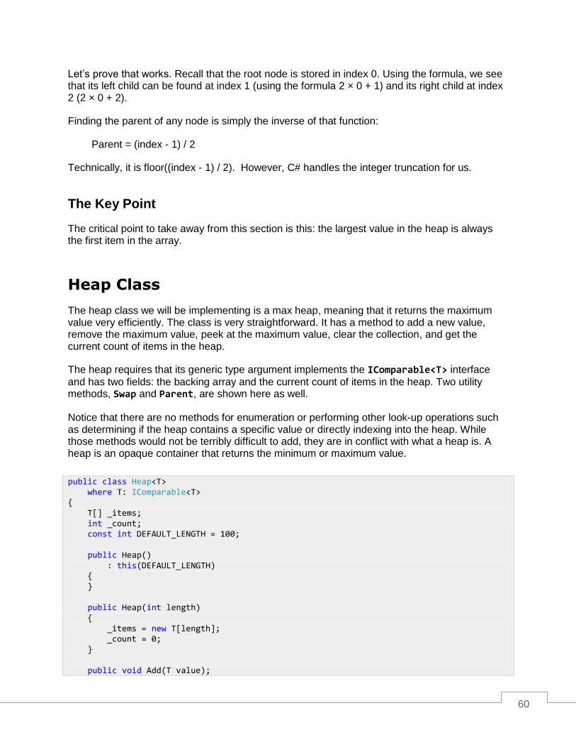
Heap Class ............................................................................................................................................ 60

Add ......................................................................................................................................................... 61

RemoveMax ........................................................................................................................................... 65

Peek ....................................................................................................................................................... 69

Count ...................................................................................................................................................... 69

Clear ....................................................................................................................................................... 69

Priority Queue ........................................................................................................................................ 70

Priority Queue Class ............................................................................................................................ 70

Usage Example .................................................................................................................................... 71

Chapter 4 AVL Tree .................................................................................................................................. 73

Balanced Tree Overview........................................................................................................................ 73

What is Node Height? .......................................................................................................................... 73

Balancing Algorithms ............................................................................................................................. 75

Right Rotation ...................................................................................................................................... 75

Left Rotation ......................................................................................................................................... 77

Right-Left Rotation ............................................................................................................................... 78

Left-Right Rotation ............................................................................................................................... 80

Heaviness and Balance Factor ............................................................................................................ 81

7

AVLTreeNode Class .............................................................................................................................. 82

Balance ................................................................................................................................................ 83

Rotation Methods ................................................................................................................................. 86

AVLTree Class ....................................................................................................................................... 87

Add ....................................................................................................................................................... 88

Contains ............................................................................................................................................... 89

Remove ................................................................................................................................................ 90

GetEnumerator .................................................................................................................................... 93

Clear .................................................................................................................................................... 95

Count ................................................................................................................................................... 95

Chapter 5 B-tree ....................................................................................................................................... 96

Overview ................................................................................................................................................ 96

B-tree Structure ...................................................................................................................................... 96

Minimal Degree .................................................................................................................................... 97

Tree Height .......................................................................................................................................... 97

Searching the Tree .............................................................................................................................. 98

Putting it Together.............................................................................................................................. 100

Balancing Operations ........................................................................................................................... 100

Pushing Down .................................................................................................................................... 100

Rotating Values .................................................................................................................................. 102

Splitting Nodes ................................................................................................................................... 104

Adding Values ...................................................................................................................................... 105

Removing Values ................................................................................................................................. 107

B-tree Node .......................................................................................................................................... 108

BTreeNode Class............................................................................................................................... 108

Adding, Removing, and Updating Values .......................................................................................... 110

Splitting Node ..................................................................................................................................... 111

8

Pushing Down .................................................................................................................................... 113

Validation ........................................................................................................................................... 115

B-tree ................................................................................................................................................... 116

BTree Class ....................................................................................................................................... 116

Add ..................................................................................................................................................... 117

Remove .............................................................................................................................................. 118

Contains ............................................................................................................................................. 126

Clear .................................................................................................................................................. 127

Count ................................................................................................................................................. 127

CopyTo .............................................................................................................................................. 128

IsReadOnly ........................................................................................................................................ 128

GetEnumerator .................................................................................................................................. 129

9

The Story behind the Succinctly Series of Books

Daniel Jebaraj, Vice President Syncfusion, Inc.

taying on the cutting edge

As many of you may know, Syncfusion is a provider of software components for the Microsoft platform. This puts us in the exciting but challenging position of always being on the cutting edge.

Whenever platforms or tools are shipping out of Microsoft, which seems to be about every other week these days, we have to educate ourselves, quickly.

Information is plentiful but harder to digest

In reality, this translates into a lot of book orders, blog searches, and Twitter scans.

While more information is becoming available on the Internet and more and more books are being published, even on topics that are relatively new, one aspect that continues to inhibit us is the inability to find concise technology overview books.

We are usually faced with two options: read several 500+ page books or scour the web for relevant blog posts and other articles. Just as everyone else who has a job to do and customers to serve, we find this quite frustrating.

The Succinctly series

This frustration translated into a deep desire to produce a series of concise technical books that would be targeted at developers working on the Microsoft platform.

We firmly believe, given the background knowledge such developers have, that most topics can be translated into books that are between 50 and 100 pages.

This is exactly what we resolved to accomplish with the Succinctly series. Isn’t everything wonderful born out of a deep desire to change things for the better?

The best authors, the best content

Each author was carefully chosen from a pool of talented experts who shared our vision. The book you now hold in your hands, and the others available in this series, are a result of the authors’ tireless work. You will find original content that is guaranteed to get you up and running in about the time it takes to drink a few cups of coffee.

S

10

Free forever

Syncfusion will be working to produce books on several topics. The books will always be free. Any updates we publish will also be free.

Free? What is the catch?

There is no catch here. Syncfusion has a vested interest in this effort.

As a component vendor, our unique claim has always been that we offer deeper and broader frameworks than anyone else on the market. Developer education greatly helps us market and sell against competing vendors who promise to “enable AJAX support with one click,” or “turn the moon to cheese!”

Let us know what you think

If you have any topics of interest, thoughts, or feedback, please feel free to send them to us at [email protected].

We sincerely hope you enjoy reading this book and that it helps you better understand the topic of study. Thank you for reading.

Please follow us on Twitter and “Like” us on Facebook to help us spread the word about the Succinctly series!

mailto:[email protected]

https://twitter.com/syncfusion

https://www.facebook.com/Syncfusion

11

Chapter 1 Skip Lists

Overview

In the previous book, we looked at two common list-like data structures: the linked list and the array list. Each data structure came with a set of trade-offs. Now I’d like to add a third into the mix: the skip list.

A skip list is an ordered (sorted) list of items stored in a linked-list structure in a way that allows O(log n) insertion, removal, and search. So it looks like an ordered list, but has the operational complexity of a balanced tree.

Why is this compelling? Doesn’t a sorted array give you O(log n) search as well? Sure, but a sorted array doesn’t give you O(log n) insertion or removal. Okay, why not just use a tree? Well, you could. But as we will see, the implementation of the skip list is much less complex than an unbalanced tree, and far less complex than a balanced one. Also, at the end of the chapter I’ll examine at another benefit of a skip list that wouldn’t be too hard to add—array-style indexing.

So if a skip list is as good as a balanced tree while being easier to implement, why don’t more people use them? I suspect it is a lack of awareness. Skip lists are a relatively new data structure—they were first documented by William Pugh in 1990—and as such are not a core part of most algorithm and data structure courses.

How it Works

Let’s start by looking at an ordered linked list in memory.

Figure 1: A sorted linked list represented in memory

I think we can all agree that searching for the value 8 would require an O(n) search that started at the first node and went to the last node.

So how can we cut that in half? Well, what if we were able to skip every other node? Obviously, we can’t get rid of the basic Next pointer—the ability to enumerate each item is critical. But what

if we had another set of pointers that skipped every other node? Now our list might look like this:

12

Figure 2: Sorted linked list with pointers skipping every other node

Our search would be able to perform one half the comparisons by using the wider links. The orange path shown in the following figure demonstrates the search path. The orange dots represent points where comparisons were performed—it is comparisons we are measuring when determining the complexity of the search algorithm.

Figure 3: Search path across new pointers

O(n) is now roughly O(n/2). That’s a decent improvement, but what would happen if we added another layer?

Figure 4: Adding an additional layer of links

We’re now down to four comparisons. If the list were nine items long, we could find the value 9 in using only O(n/3) comparisons.

With each additional layer of links, we can skip more and more nodes. This layer skipped three. The next would skip seven. The one after that skips 15 at a time.

13

Going back to Figure 4, let’s look at the specific algorithm that was used.

We started at the highest link on the first node. Since that node’s value (1) did not match the value we sought (8), we checked the value the link pointed to (5). Since 5 was less than the value we wanted, we went to that node and repeated the process.

The 5 node had no additional links at the third level, so we went down to level two. Level two had a link so we compared what it pointed to (7) against our sought value (8). Since the value 7 was less than 8, we followed that link and repeated.

The 7 node had no additional links at the second level so we went down to the first level and compared the value the link pointed to (8) with the value we sought (8). We found our match.

While the mechanics are new, this method of searching should be familiar. It is a divide and conquer algorithm. Each time we followed a link we were essentially cutting the search space in half.

But There is a Problem

There is a problem with the approach we took in the previous example. The example used a deterministic approach to setting the link level height. In a static list this might be acceptable, but as nodes are added and removed, we can quickly create pathologically bad lists that become degenerate linked lists with O(n) performance.

Let’s take our three-level skip list and remove the node with the value 5 from the list.

Figure 5: Skip list with 5 node removed

With 5 gone, our ability to traverse the third-level links is gone, but we’re still able to find the value 8 in four comparisons (basically O(n/2)). Now let’s remove 7.

14

Figure 6: Skip list with 5 and 7 nodes removed

We can now only use a single level-two link and our algorithm is quickly approaching O(n). Once we remove the node with the value 3, we will be there.

Figure 7: Skip list with 3, 5, and 7 nodes removed

And there we have it. With a series of three carefully planned deletions, the search algorithm went from being O(n/3) to O(n).

To be clear, the problem is not that this situation can happen, but rather that the situation could be intentionally created by an attacker. If a caller has knowledge about the patterns used to create the skip list structure, then he or she could craft a series of operations that create a scenario like what was just described.

The easiest way to mitigate this, but not entirely prevent it, is to use a randomized height approach. Basically, we want to create a strategy that says that 100% of nodes have the first-level link (this is mandatory since we need to be able to enumerate every node in order), 50% of the nodes have the second level, 25% have the third level, etc. Because a random approach is, well, random, it won’t be true that exactly 50% or 25% have the second or third levels, but over time, and as the list grows, this will become true.

Using a randomized approach, our list might look something like this:

15

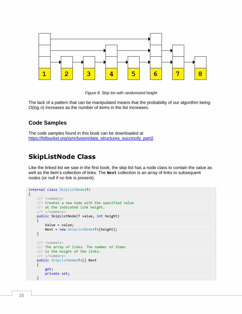
Figure 8: Skip list with randomized height

The lack of a pattern that can be manipulated means that the probability of our algorithm being O(log n) increases as the number of items in the list increases.

Code Samples

The code samples found in this book can be downloaded at https://bitbucket.org/syncfusion/data_structures_succinctly_part2.

SkipListNode Class

Like the linked list we saw in the first book, the skip list has a node class to contain the value as well as the item’s collection of links. The Next collection is an array of links to subsequent

nodes (or null if no link is present).

internal class SkipListNode<T> { /// <summary> /// Creates a new node with the specified value /// at the indicated link height. /// </summary> public SkipListNode(T value, int height) { Value = value; Next = new SkipListNode<T>[height]; } /// <summary> /// The array of links. The number of items /// is the height of the links. /// </summary> public SkipListNode<T>[] Next { get; private set; }

https://bitbucket.org/syncfusion/data_structures_succinctly_part2

16

SkipList Class

The SkipList<T> class is a generic class that implements the ICollection<T> interface and

requires the generic type argument, T, be of a type that implements the IComparable<T>

interface. Since skip lists are an ordered collection, it is a requirement that the contained type implements the IComparable<T> interface.

There are a few private fields in addition to the ICollection<T> method and properties. The

_rand field provides access to a random number generator that will be used to randomly

determine the node link height. The _head field is a node which does not contain any data, but

has a maximum link height—this is important because it will serve as a starting point for all traversals. The _levels field is the current maximum link height in use by any node (not

including the _head node). _count is the number of items contained in the list.

The remaining methods and properties are required to implement the ICollection<T>

interface:

/// <summary> /// The contained value. /// </summary> public T Value { get; private set; } }

public class SkipList<T> : ICollection<T> where T: IComparable<T> { // Used to determine the random height of the node links. private readonly Random _rand = new Random(); // The non-data node which starts the list. private SkipListNode<T> _head; // There is always one level of depth (the base list). private int _levels = 1; // The number of items currently in the list. private int _count = 0; public SkipList() {} public void Add(T value) {} public bool Contains(T value) { throw new NotImplementedException(); } public bool Remove(T value) { throw new NotImplementedException(); } public void Clear() {}

17

Add

Behavior Adds the specific value to the skip list.

Performance O(log n)

The add algorithm for skip lists is fairly simple:

1. Pick a random height for the node (PickRandomLevel method).

2. Allocate a node with the random height and a specific value.

3. Find the appropriate place to insert the node into the sorted list.

4. Insert the node.

Picking a Level

As stated previously, the random height needs to be scaled logarithmically. 100% of the values must be at least 1—a height of 1 is the minimum needed for a regular linked list. 50% of the heights should be 2. 25% should be level 3, and so on.

Any algorithm that satisfies this scaling is suitable. The algorithm demonstrated here uses a random 32-bit value and the generated bit pattern to determine the height. The index of the first LSB bit that is a 1, rather than a 0, is the height that will be used.

Let’s look at the process by reducing the set from 32 bits to 4 bits, and looking at the 16 possible values and the height from that value.

Bit Pattern Height Bit Pattern Height

0000 5 1000 4

public void CopyTo(T[] array, int arrayIndex) {} public int Count { get { throw new NotImplementedException(); } } public bool IsReadOnly { get { throw new NotImplementedException(); } } public IEnumerator<T> GetEnumerator() { throw new NotImplementedException(); } System.Collections.IEnumerator System.Collections.IEnumerable.GetEnumerator() { throw new NotImplementedException(); } }

18

Bit Pattern Height Bit Pattern Height

0001 1 1001 1

0010 2 1010 2

0011 1 1011 1

0100 3 1100 3

0101 1 1101 1

0110 2 1110 2

0111 1 1111 1

With these 16 values, you can see the distribution works as we expect. 100% of the heights are at least 1. 50% are at least height 2.

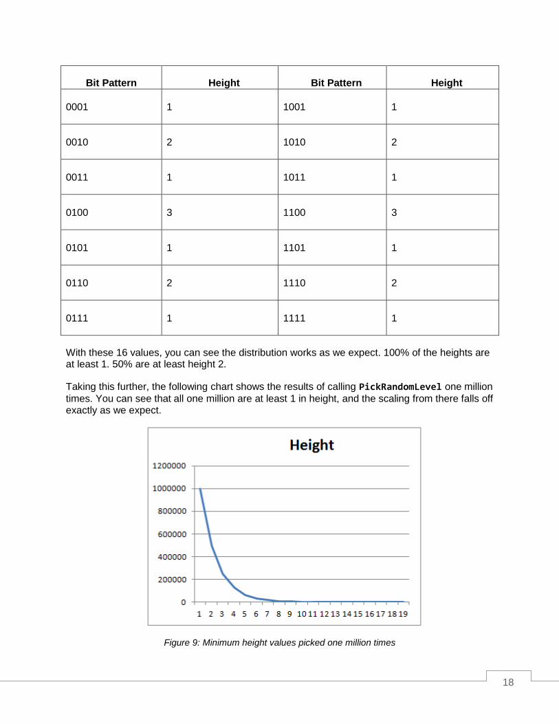
Taking this further, the following chart shows the results of calling PickRandomLevel one million

times. You can see that all one million are at least 1 in height, and the scaling from there falls off exactly as we expect.

Figure 9: Minimum height values picked one million times

19

Picking the Insertion Point

The insertion point is found using the same algorithm described for the Contains method. The

primary difference is that at the point where Contains would return true or false, the following is

true:

1. The current node is less than or equal to the value being inserted.

2. The next node is greater than or equal to the value being inserted.

This is a valid point to insert the new node.

public void Add(T item) { int level = PickRandomLevel(); SkipListNode<T> newNode = new SkipListNode<T>(item, level + 1); SkipListNode<T> current = _head; for (int i = _levels - 1; i >= 0; i--) { while (current.Next[i] != null) { if (current.Next[i].Value.CompareTo(item) > 0) { break; } current = current.Next[i]; } if (i <= level) { // Adding "c" to the list: a -> b -> d -> e. // Current is node b and current.Next[i] is d. // 1. Link the new node (c) to the existing node (d): // c.Next = d newNode.Next[i] = current.Next[i]; // Insert c into the list after b: // b.Next = c current.Next[i] = newNode; } } _count++; } private int PickRandomLevel() { int rand = _rand.Next(); int level = 0; // We're using the bit mask of a random integer to determine if the max

20

Remove

Behavior Removes the first node with the indicated value from the skip list.


The Remove operation determines if the node being searched for exists in the list and, if so,

removes it from the list using the normal linked list item removal algorithm.

The search algorithm used is the same method described for the Contains method.

// level should increase by one or not. // Say the 8 LSBs of the int are 00101100. In that case, when the // LSB is compared against 1, it tests to 0 and the while loop is never // entered so the level stays the same. That should happen 1/2 of the time. // Later, if the _levels field is set to 3 and the rand value is 01101111, // the while loop will run 4 times and on the last iteration will // run another 4 times, creating a node with a skip list height of 4. This should // only happen 1/16 of the time. while ((rand & 1) == 1) { if (level == _levels) { _levels++; break; } rand >>= 1; level++; } return level; }

public bool Remove(T item) { SkipListNode<T> cur = _head; bool removed = false; // Walk down each level in the list (make big jumps). for (int level = _levels - 1; level >= 0; level--) { // While we're not at the end of the list: while (cur.Next[level] != null) { // If we found our node, if (cur.Next[level].Value.CompareTo(item) == 0) { // remove the node,

21

Contains

Behavior Returns true if the value being sought exists in the skip list.


The Contains operation starts at the tallest link on the first node and checks the value at the

end of the link. If that value is less than or equal to the sought value, the link can be followed; but if the linked value is greater than the sought value, we need to drop down one height level and try the next link there. Eventually, we will either find the value we seek or we will find that the node does not exist in the list.

The following image demonstrates how the number 5 is searched for within the skip list.

cur.Next[level] = cur.Next[level].Next[level]; removed = true; // and go down to the next level (where // we will find our node again if we're // not at the bottom level). break; } // If we went too far, go down a level. if (cur.Next[level].Value.CompareTo(item) > 0) { break; } cur = cur.Next[level]; } } if (removed) { _count--; } return removed; }

22

Figure 10: Searching a skip list for the value 5

The first comparison is performed at the topmost link. The linked value, 6, is greater than the value being sought (5), so instead of following the link the search repeats at the next lower height.

The next lower link is connected to a node with the value 4. This is less than the value being sought, so the link is followed.

The 4 node at height 2 is linked to the node with the value 6. Since this is greater than the value we're looking for, the link cannot be followed and the search cycle repeats at the next lower level.

At this point, the link points to the node containing the value 5, which is the value we sought.

public bool Contains(T item) { SkipListNode<T> cur = _head; for (int i = _levels - 1; i >= 0; i--) { while (cur.Next[i] != null) { int cmp = cur.Next[i].Value.CompareTo(item); if (cmp > 0) { // The value is too large, so go down one level // and take smaller steps. break; } if (cmp == 0) { // Found it! return true; } cur = cur.Next[i]; }

23

Clear

Behavior Removes all the entries in the list.

Performance O(1)

Clear reinitializes the head of the list and sets the current count to 0.

CopyTo

Behavior Copies the contents of the skip list into the provided array starting at the specified array index.

Performance O(n)

The CopyTo method uses the class enumerator to enumerate the items in the list and copies

each item into the target array.

} return false; }

public void Clear() { _head = new SkipListNode<T>(default(T), 32 + 1); _count = 0; }

public void CopyTo(T[] array, int arrayIndex) { if (array == null) { throw new ArgumentNullException("array"); } int offset = 0; foreach (T item in this) { array[arrayIndex + offset++] = item; } }

24

IsReadOnly

Behavior Returns a value indicating if the skip list is read only.

Performance O(1)

In this implementation, the skip list is hardcoded not to be read-only.

Count

Behavior Returns the current number of items in the skip list (zero if empty).

Performance O(1)

GetEnumerator

Behavior Returns an IEnumerator<T> instance that can be used to enumerate the

items in the skip list in sorted order.

Performance O(1) to return the enumerator; O(n) to perform the enumeration (caller cost).

The enumeration method simply walks the list at height 1 (array index 0). This is the list whose links are always to the next node in the list.

public bool IsReadOnly { get { return false; } }

public int Count { get { return _count; } }

public IEnumerator<T> GetEnumerator() {

25

Common Variations

Array-Style Indexing

A common change made to the skip list is to provide index-based item access; for example, the n-th item could be accessed by the caller using array-indexing syntax.

This could easily be implemented in O(n) time by simply walking the first level links, but an optimized approach would be to track the length of each link and use that information to walk to the appropriate link. An example list might be visualized like this:

Figure 11: A skip list with link lengths

With these lengths we can implement array-like indexing in O(log n) time—it uses the same algorithm as the Contains method, but instead of checking the value on the end of the link we

simply check the link length.

Making this change is not terribly difficult, but it is a little more complex than simply adding the length attribute. The Add and Remove methods need to be updated to set the length of all

affected links, at all heights, after each operation.

SkipListNode<T> cur = _head.Next[0]; while (cur != null) { yield return cur.Value; cur = cur.Next[0]; } } System.Collections.IEnumerator System.Collections.IEnumerable.GetEnumerator() { return GetEnumerator(); }

26

Set behaviors

Another common change is to implement a Set (or Set-like behaviors) by not allowing duplicate

values in the list. Because this is a relatively common usage of skip lists, it is important to understand how your list handles duplicates before using it.

27

Chapter 2 Hash Table

Hash Table Overview

Hash tables are a collection type that store key–value pairs in a manner that provides fast insertion, lookup, and removal operations. Hash tables are commonly used in, but certainly not limited to, the implementation of associative arrays and data caches. For example, a website might keep track of active sessions in a hash table using the following pattern:

In this example, a hash table is being used to store session state using the session ID as the key and the session state as the value. When the session state is sought in the hash table, if it is not found, a new session state object is added and, in either case, the state that matches the session ID is returned.

Using a hash table in this manner allows fast insertion and retrieval (on average) of the session state, regardless of how many active sessions are occurring concurrently.

Hashing Basics

Overview

The Key and Value

To understand how a hash table works, let’s look at a conceptual overview of adding an item to a hash table and then finding that item.

The object we’ll be storing (shown in JSON format) represents an employee at a company.

HashTable<string, SessionState> _sessionStateCache; ... public SessionState LoadSession(string sessionId) { SessionState state; if (!_sessionStateCache.TryGetValue(sessionId, out state)) { state = new SessionState(sessionId); _sessionStateCache[sessionId] = state; } return state; }

28

Recall that to store an item in a hash table, we need to have both a key and a value. Our object is the value, so now we need to pick a key. Ideally we would pick something that can uniquely represent the object being stored; however, in this case we will use the employee name (Robert Horvick) to demonstrate that the key can be any data type. In practice, the Employee

class would contain a unique ID that distinguishes between multiple employees who share the same name, and that ID would be the key we use.

The Backing Array

For fast access to items, hash tables are backed by an array (O(1) random access) rather than a list (O(n) random access). At any given moment, the array has two properties that are interesting:

1. Capacity

2. Fill Factor

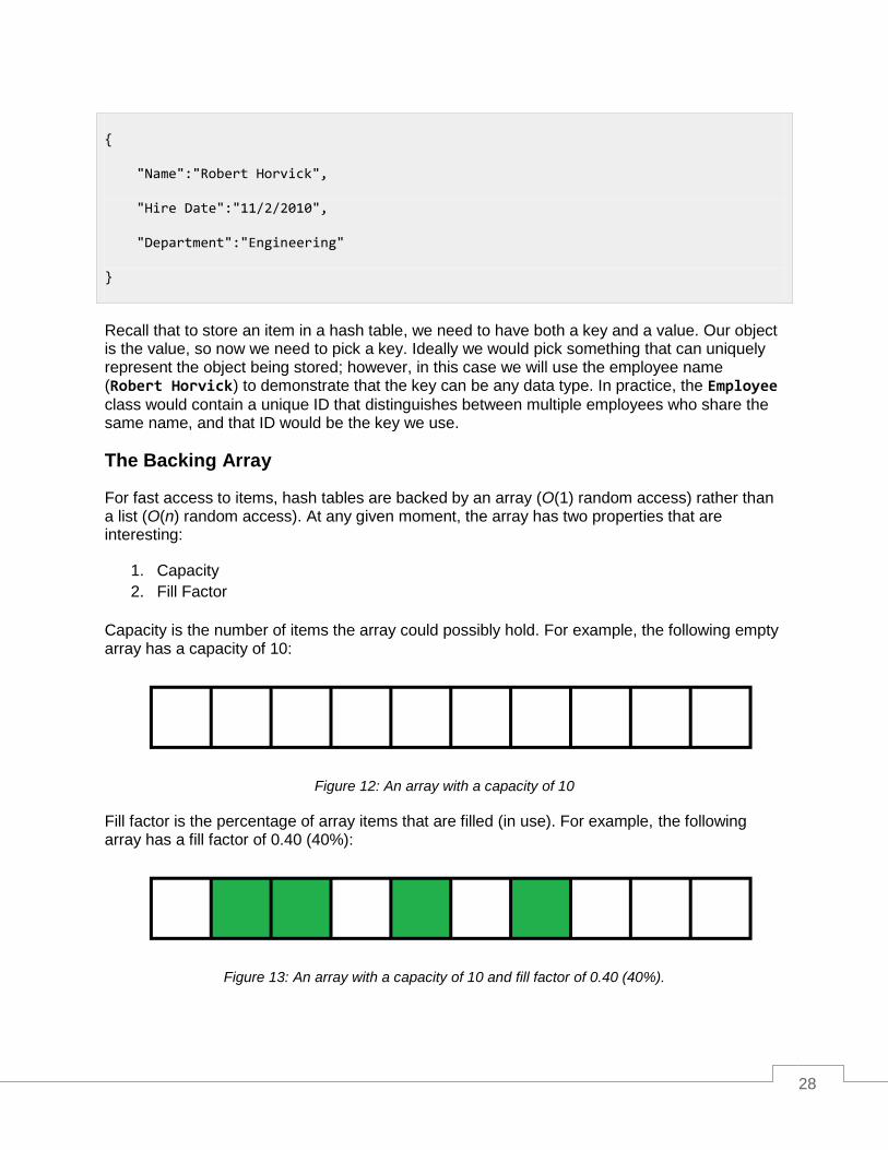
Capacity is the number of items the array could possibly hold. For example, the following empty array has a capacity of 10:

Figure 12: An array with a capacity of 10

Fill factor is the percentage of array items that are filled (in use). For example, the following array has a fill factor of 0.40 (40%):

Figure 13: An array with a capacity of 10 and fill factor of 0.40 (40%).

{

"Name":"Robert Horvick",

"Hire Date":"11/2/2010",

"Department":"Engineering"

}

29

Notice that the array is filled in an apparently random manner. While the array contains four items, the items are not stored in indexes 0–3, but rather 1, 2, 4, and 6. This is because the index at which an item is stored is determined by a hash function which takes the key component—Robert Horvick, in our example—and returns an integer hash code. This hash

code will then be fit into the array’s size using the modulo operation. For example:

Hashing Algorithms

The previous code sample makes a call to a function named hash, which accepts a string and

returns an integer. This integer is the hash code of the provided string.

Before we go further, let’s take a moment to consider just how important hash codes are. The .NET framework requires that all classes derive from the base type System.Object. This type

provides the base implementation of several methods, one of which has the following signature:

Putting this method on the common base type ensures that every type will be able to produce a hash code and therefore be capable of being stored in a collection type that requires a hash code.

The question, then, is what should the hash code for any given object instance be? How does a System.String with a value like "Robert Horvick" produce an integer value suitable for being

used as a hash code?

The function needs to have two properties. First, the hash algorithm must be stable. This means that given the same input, the same hash value will always be returned. Second, the hash algorithm must be uniform. This means that hash function maps input values to output values in a manner that is evenly (uniformly) distributed through the entire output range.

Here is a (bad) example:

int index = hash(“Robert Horvick”) % Capacity;

int GetHashCode()

public int LengthHashCode(string input) { return input.Length; }

30

This hash code method returns the length of the string as the hash code. This method is stable. The string "Robert Horvick" will always return the same hash code (14). But this method does not have uniform distribution. What would happen if we had one million unique strings, each of which was 50 characters long? Each of them would have a hash code of 50. This is not a uniform distribution, and therefore not a suitable hash algorithm for strings.

Here’s a slightly better (bad) example:

This hash function has only slightly better uniformity than the length-based hash. While an additive hash does allow same-length strings produce different hashes, it also means that “Robert Horvick” and “Horvick Robert” will both produce the same hash value.

Now that we know what a poor hashing algorithm looks like, let’s take a look at a significantly better string hashing algorithm. This algorithm was first reported by Dan Bernstein (http://www.cse.yorku.ca/~oz/hash.html) and uses an algorithm that, for each character in the value to hash (c), sets the current hash value to hash = (hash * 33) + c.

private int AdditiveHash(string input) { int currentHashValue = 0; foreach (char c in input) { unchecked { currentHashValue += (int)c; } } return currentHashValue; }

// Hashing function first reported by Dan Bernstein. // http://www.cse.yorku.ca/~oz/hash.html private static int Djb2(string input) { int hash = 5381; foreach (int c in input.ToCharArray()) { unchecked { /* hash * 33 + c */ hash = ((hash << 5) + hash) + c; } } return hash; }

http://www.cse.yorku.ca/~oz/hash.html

31

Just for fun, let’s look at one more hash algorithm. This hash algorithm, known as a folding hash, does not process the string character by character, but rather in 4-byte blocks. Let’s take a look at how the ASCII string “Robert Horvick” would be hashed. First, the string is broken up into 4-byte blocks. Since we are using ASCII encoding, each character is one block, and so the segments are:

Each of those characters is represented by a 1-byte numeric ASCII code. Those bytes are:

These bytes are then stuffed into 32-bit values (the bytes are reversed here due to how they are loaded into the resulting integer. See the GetNextBytes method in the sample code.)

The values are summed, allowing overflow to occur, and we are given the final hash value: 0x16F9C196.

[Robe]

[rt H]

[orvi]

[ck]

[0x52 0x6F 0x62 0x65]

[0x72 0x74 0x20 0x48]

[0x6F 0x72 0x76 0x69]

[0x63 0x6B]

0x65626F52

0x48207472

0x6976726F

0x00006B63

// Treats each four characters as an integer, so // "aaaabbbb" hashes differently than "bbbbaaaa". private static int FoldingHash(string input) { int hashValue = 0; int startIndex = 0;

32

The last two hashing functions are conceptually simple and also simple to implement. But how good are they? I created a simple test that generated one million unique values by converting GUIDs to strings. I then hashed those one million unique strings and recorded the number of hash collisions, which occur when two distinct values have the same hash value. The results were:

DJB2 unique values: 99.88282%

Folding unique values: 97.75495%

As you can see, both hash algorithms distributed the hash values relatively evenly with DJB2 having slightly better distribution than the folding hash.

int currentFourBytes; do { currentFourBytes = GetNextBytes(startIndex, input); unchecked { hashValue += currentFourBytes; } startIndex += 4; } while (currentFourBytes != 0); return hashValue; } // Gets the next four bytes of the string converted to an // integer. If there are not enough characters, 0 is used. private static int GetNextBytes(int startIndex, string str) { int currentFourBytes = 0; currentFourBytes += GetByte(str, startIndex); currentFourBytes += GetByte(str, startIndex + 1) << 8; currentFourBytes += GetByte(str, startIndex + 2) << 16; currentFourBytes += GetByte(str, startIndex + 3) << 24; return currentFourBytes; } private static int GetByte(string str, int index) { if (index < str.Length) { return (int)str[index]; } return 0; }

33

Handling Collisions

As we saw in the previous section, a good hashing algorithm is one that will distribute the hashed values evenly over the possible range of hash values, but we also saw that even a good algorithm will likely produce a collision. Further, we know that the hash value will eventually be fit into the backing array size using the modulo operator, so even a perfect hashing algorithm may eventually have collisions when the hash value is fit into the backing array size.

Next Open Slot

The next open slot method walks forward in the backing array searching for the next open slot and places the item in that location. For example, in the following figure, the values V1 and V2 have the same hash value. Since V1 is already in the hash table, V2 moves forward to the next open slot in the hash table.

Figure 14: Collisions of the hash values for V1 and V2

During the look-up process, if the value V2 is sought, the index for V1 will be found. The value of V1 and V2 will be compared and they will not match. Since next-slot collision handling is being used, the hash table needs to check the next index to determine if a collision was moved forward. In the next slot, the value V2 is found and compared to the sought value, V2. Since they are the same, the appropriate backing array index has been found.

We can see that this method has simple insertion and search rules, but unfortunately has complex removal logic.

Consider what would happen if V1 were removed: The third index, which V1 was in, is now empty. If a search for V2 were performed, the expected index would be empty so it would be assumed V2 is not in the hash table, even though it is. This means that during the removal process, all values adjacent to the item being removed need to be checked to see if they need to be moved.

34

One trade-off of this collision handling algorithm is that removals are complex, but the entire hash table is stored in a single, contiguous backing array. This might make it attractive on systems where memory resources are limited, or where data locality in memory is extremely important.

Linked List Chains

Another method of handling collisions is to have each index in the hash table backing array be a linked list of nodes. When a collision occurs, the new value is added to the linked list. For example:

Figure 15: V2 is added to the linked list after V1

With a language that supports union types (e.g., C++), the array index will typically contain a value that can be either the single value when there have not been any collisions, or a linked list. The sample code in the next section will always create a linked list, but will only do so when an item is added at the index.

HashTableNodePair Class

The HashTableNodePair class is the key–value pair stored within the hash table array. Unlike

the .NET Framework KeyValuePair class, the HashTableNodePair does not allow the key

member to be assigned after construction, because that value is used to determine the index in the hash table where the key–value pair is stored.

/// <summary>

/// A node in the hash table array.

/// </summary>

35

/// <typeparam name="TKey">The type of the key of the key/value pair.</typeparam>

/// <typeparam name="TValue">The type of the value of the key/value pair.</typeparam>

public class HashTableNodePair<TKey, TValue>

{

/// <summary>

/// Constructs a key/value pair for storage in the hash table.

/// </summary>

/// <param name="key">The key of the key/value pair.</param>

/// <param name="value">The value of the key/value pair.</param>

public HashTableNodePair(TKey key, TValue value)

{

Key = key;

Value = value;

}

/// <summary>

/// The key. The key cannot be changed because it would affect the

/// indexing in the hash table.

/// </summary>

public TKey Key { get; private set; }

/// <summary>

/// The value.

/// </summary>

public TValue Value { get; set; }

}

36

HashTableArrayNode Class

The HashTableArrayNode class represents a single node within the hash table. It performs a

lazy initialization of the linked list used for handling collisions. It provides methods for adding, removing, updating, and retrieving the key–value pairs stored in the node. Additionally, it provides enumeration of the keys and values in order to support the hash table’s enumeration requirements.

Add

Behavior Adds the key–value pair to the node, lazily initializing the linked list when addi|ng the first value. If the key being added already exists, an exception is thrown.

Performance O(1)

internal class HashTableArrayNode<TKey, TValue> { // This list contains the actual data in the hash table. It chains together // data collisions. LinkedList<HashTableNodePair<TKey, TValue>> _items; public void Add(TKey key, TValue value); public void Update(TKey key, TValue value); public bool TryGetValue(TKey key, out TValue value); public bool Remove(TKey key); public void Clear(); public IEnumerable<TValue> Values { get; } public IEnumerable<TKey> Keys { get; } public IEnumerable<HashTableNodePair<TKey, TValue>> Items { get; } }

/// <summary> /// Adds the key/value pair to the node. If the key already exists in the /// list, an ArgumentException will be thrown. /// </summary> /// <param name="key">The key of the item being added.</param> /// <param name="value">The value of the item being added.</param> public void Add(TKey key, TValue value) {

37

Update

Behavior Finds the key–value pair with the matching key and updates the associated value. If the key is not found, an exception is thrown.

Performance O(n), where n is the number of values in the linked list. In general this will be an O(1) algorithm because there will not be a collision.

// Lazy init the linked list. if (_items == null) { _items = new LinkedList<HashTableNodePair<TKey, TValue>>(); } else { // Multiple items might collide and exist in this list, but each // key should only be in the list once. foreach (HashTableNodePair<TKey, TValue> pair in _items) { if (pair.Key.Equals(key)) { throw new ArgumentException("The collection already contains the key"); } } } // If we made it this far, add the item. _items.AddFirst(new HashTableNodePair<TKey, TValue>(key, value)); }

/// <summary> /// Updates the value of the existing key/value pair in the list. /// If the key does not exist in the list, an ArgumentException /// will be thrown. /// </summary> /// <param name="key">The key of the item being updated.</param> /// <param name="value">The updated value.</param> public void Update(TKey key, TValue value) { bool updated = false; if (_items != null) { // Check each item in the list for the specified key. foreach (HashTableNodePair<TKey, TValue> pair in _items) { if (pair.Key.Equals(key)) {

38

TryGetValue

Behavior Sets the out parameter value to the value associated with the provided key and returns true if the key is found. Otherwise it returns false.

Performance O(n), where n is the number of values in the linked list. In general, this will be an O(1) algorithm because there will not be a collision.

// Update the value. pair.Value = value; updated = true; break; } } } if (!updated) { throw new ArgumentException("The collection does not contain the key."); } }

/// <summary> /// Finds and returns the value for the specified key. /// </summary> /// <param name="key">The key whose value is sought.</param> /// <param name="value">The value associated with the specified key.</param> /// <returns>True if the value was found, false otherwise.</returns> public bool TryGetValue(TKey key, out TValue value) { value = default(TValue); bool found = false; if (_items != null) { foreach (HashTableNodePair<TKey, TValue> pair in _items) { if (pair.Key.Equals(key)) { value = pair.Value; found = true; break; } } } return found; }

39

Remove

Behavior Finds the key–value pair with the matching key and removes the key–value pair from the linked list. If the pair is removed, the value true is returned.

Otherwise it returns false.

Performance O(n), where n is the number of values in the linked list. In general, this will be an O(1) algorithm because there will not be a collision.

/// <summary> /// Removes the item from the list whose key matches /// the specified key. /// </summary> /// <param name="key">The key of the item to remove.</param> /// <returns>True if the item is removed; false otherwise.</returns> public bool Remove(TKey key) { bool removed = false; if (_items != null) { LinkedListNode<HashTableNodePair<TKey, TValue>> current = _items.First; while (current != null) { if (current.Value.Key.Equals(key)) { _items.Remove(current); removed = true; break; } current = current.Next; } } return removed; }

40

Clear

Behavior Removes all the items from the linked list.

Note: This implementation simply clears the linked list; however, it would also be possible to assign the _items reference to null and let the garbage

collector reclaim the memory. The next call to Add would allocate a new linked

list.

Performance O(1)

Enumeration

Keys

Behavior Returns an enumerator that enumerates the keys in the linked list.

Performance O(1)

/// <summary> /// Removes all the items from the list. /// </summary> public void Clear() { if (_items != null) { _items.Clear(); } }

/// <summary> /// Returns an enumerator for all of the keys in the list. /// </summary> public IEnumerable<TKey> Keys { get { if (_items != null) { foreach (HashTableNodePair<TKey, TValue> node in _items) { yield return node.Key;

41

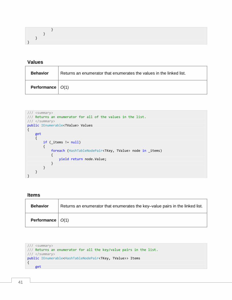
Values

Behavior Returns an enumerator that enumerates the values in the linked list.

Performance O(1)

Items

Behavior Returns an enumerator that enumerates the key–value pairs in the linked list.

Performance O(1)

} } } }

/// <summary> /// Returns an enumerator for all of the values in the list. /// </summary> public IEnumerable<TValue> Values { get { if (_items != null) { foreach (HashTableNodePair<TKey, TValue> node in _items) { yield return node.Value; } } } }

/// <summary> /// Returns an enumerator for all the key/value pairs in the list. /// </summary> public IEnumerable<HashTableNodePair<TKey, TValue>> Items { get

42

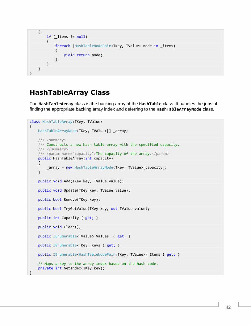
HashTableArray Class

The HashTableArray class is the backing array of the HashTable class. It handles the jobs of

finding the appropriate backing array index and deferring to the HashTableArrayNode class.

{ if (_items != null) { foreach (HashTableNodePair<TKey, TValue> node in _items) { yield return node; } } } }

class HashTableArray<TKey, TValue> { HashTableArrayNode<TKey, TValue>[] _array; /// <summary> /// Constructs a new hash table array with the specified capacity. /// </summary> /// <param name="capacity">The capacity of the array.</param> public HashTableArray(int capacity) { _array = new HashTableArrayNode<TKey, TValue>[capacity]; } public void Add(TKey key, TValue value); public void Update(TKey key, TValue value); public bool Remove(TKey key); public bool TryGetValue(TKey key, out TValue value); public int Capacity { get; } public void Clear(); public IEnumerable<TValue> Values { get; } public IEnumerable<TKey> Keys { get; } public IEnumerable<HashTableNodePair<TKey, TValue>> Items { get; } // Maps a key to the array index based on the hash code. private int GetIndex(TKey key); }

43

Add

Behavior Adds the key–value pair to the node array. If the key already exists in the node array, an exception will be thrown.

Performance O(1)

The main purpose of this method is to lazily allocate the HashTableArrayNode instance so that

only hash table entries that actually hold a value allocate an instance.

Update

Behavior Updates the value of the key–value pair whose key matches the provided key. If the key does not exist, an exception is thrown.

Performance O(n), where n is the number of items stored in the HashTableNodeArray

instance. This will typically be an O(1) operation.

/// <summary> /// Adds the key/value pair to the node. If the key already exists in the /// node array, an ArgumentException will be thrown. /// </summary> /// <param name="key">The key of the item being added.</param> /// <param name="value">The value of the item being added.</param> public void Add(TKey key, TValue value) { int index = GetIndex(key); HashTableArrayNode<TKey, TValue> nodes = _array[index]; if (nodes == null) { nodes = new HashTableArrayNode<TKey, TValue>(); _array[index] = nodes; } nodes.Add(key, value); }

/// <summary> /// Updates the value of the existing key/value pair in the node array. /// If the key does not exist in the array, an ArgumentException /// will be thrown. /// </summary> /// <param name="key">The key of the item being updated.</param>

44

TryGetValue

Behavior Finds the value associated with the provided key and sets the out parameter to that value (else the default value for the contained type). Returns true if

the value is found. Otherwise it returns false.



Remove

Behavior Removes the key–value pair whose key matches the provided key. Returns true if the key is found and removed. Otherwise it returns false.

/// <param name="value">The updated value.</param> public void Update(TKey key, TValue value) { HashTableArrayNode<TKey, TValue> nodes = _array[GetIndex(key)]; if (nodes == null) { throw new ArgumentException("The key does not exist in the hash table", "key"); } nodes.Update(key, value); }

/// <summary> /// Finds and returns the value for the specified key. /// </summary> /// <param name="key">The key whose value is sought.</param> /// <param name="value">The value associated with the specified key.</param> /// <returns>True if the value is found; false otherwise.</returns> public bool TryGetValue(TKey key, out TValue value) { HashTableArrayNode<TKey, TValue> nodes = _array[GetIndex(key)]; if (nodes != null) { return nodes.TryGetValue(key, out value); } value = default(TValue); return false; }

45



GetIndex

Behavior Returns the index in the backing array the key hashes to.

Performance O(1)

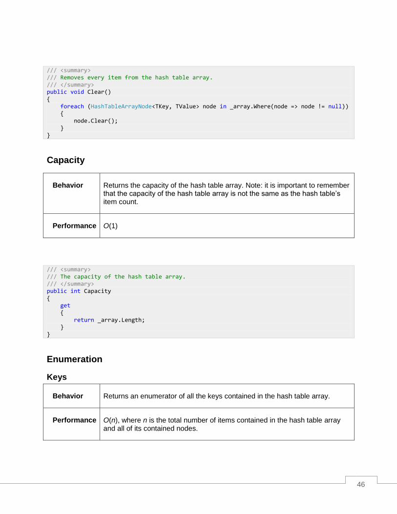
Clear

Behavior Removes all items from the hash table array.

Performance O(n), where n is the number of nodes in the table that contain data.

/// <summary> /// Removes the item from the node array whose key matches /// the specified key. /// </summary> /// <param name="key">The key of the item to remove.</param> /// <returns>True if the item was removed; false otherwise.</returns> public bool Remove(TKey key) { HashTableArrayNode<TKey, TValue> nodes = _array[GetIndex(key)]; if (nodes != null) { return nodes.Remove(key); } return false; }

// Maps a key to the array index based on the hash code. private int GetIndex(TKey key) { return Math.Abs(key.GetHashCode() % Capacity); }

46

Capacity

Behavior Returns the capacity of the hash table array. Note: it is important to remember that the capacity of the hash table array is not the same as the hash table’s item count.

Performance O(1)

Enumeration

Keys

Behavior Returns an enumerator of all the keys contained in the hash table array.

Performance O(n), where n is the total number of items contained in the hash table array and all of its contained nodes.

/// <summary> /// Removes every item from the hash table array. /// </summary> public void Clear() { foreach (HashTableArrayNode<TKey, TValue> node in _array.Where(node => node != null)) { node.Clear(); } }

/// <summary> /// The capacity of the hash table array. /// </summary> public int Capacity { get { return _array.Length; } }

47

Values

Behavior Returns an enumerator of all the values contained in the hash table array.


/// <summary> /// Returns an enumerator for all of the keys in the node array. /// </summary> public IEnumerable<TKey> Keys { get { foreach (HashTableArrayNode<TKey, TValue> node in _array.Where(node => node != null)) { foreach (TKey key in node.Keys) { yield return key; } } } }

/// <summary> /// Returns an enumerator for all of the values in the node array. /// </summary> public IEnumerable<TValue> Values { get { foreach (HashTableArrayNode<TKey, TValue> node in _array.Where(node => node != null)) { foreach (TValue value in node.Values) { yield return value; } } } }

48

Items

Behavior Returns an enumerator of all the key–value pairs contained in the hash table array.


HashTable Class

/// <summary> /// Returns an enumerator for all of the Items in the node array. /// </summary> public IEnumerable<HashTableNodePair<TKey, TValue>> Items { get { foreach (HashTableArrayNode<TKey, TValue> node in _array.Where(node => node != null)) { foreach (HashTableNodePair<TKey, TValue> pair in node.Items) { yield return pair; } } } }

public class HashTable<TKey, TValue> { // If the array exceeds this fill percentage, it will grow. const double _fillFactor = 0.75; // The maximum number of items to store before growing. // This is just a cached value of the fill factor calculation. int _maxItemsAtCurrentSize; // The number of items in the hash table. int _count; // The array where the items are stored. HashTableArray<TKey, TValue> _array; /// <summary> /// Constructs a hash table with the default capacity. /// </summary> public HashTable() : this(1000)

49

Add

Behavior Adds a key–value pair to the hash table, throwing an exception if the key already exists in the table.

Performance O(1) on average. O(n + 1) when array growth occurs.

This method provides a level of abstraction over the HashTableArray class to deal with

growing the backing array when the add operation exceeds the maximum capacity. When growing the backing array, it uses the fill factor to determine the maximum item count given the current backing array capacity.

{ } /// <summary> /// Constructs a hash table with the specified capacity. /// </summary> public HashTable(int initialCapacity) { if (initialCapacity < 1) { throw new ArgumentOutOfRangeException("initialCapacity"); } _array = new HashTableArray<TKey, TValue>(initialCapacity); // When the count exceeds this value, the next Add will cause the // array to grow. _maxItemsAtCurrentSize = (int)(initialCapacity * _fillFactor) + 1; } public void Add(TKey key, TValue value); public bool Remove(TKey key); public TValue this[TKey key] { get; set; } public bool TryGetValue(TKey key, out TValue value); public bool ContainsKey(TKey key); public bool ContainsValue(TValue value); public IEnumerable<TKey> Keys { get; } public IEnumerable<TValue> Values { get; } public void Clear(); public int Count { get; } }

/// <summary> /// Adds the key/value pair to the hash table. If the key already exists in the /// hash table, an ArgumentException will be thrown. /// </summary> /// <param name="key">The key of the item being added.</param> /// <param name="value">The value of the item being added.</param>

50

Indexing

Behavior Retrieves the value with the provided key. If the key does not exist in the hash table, an exception is thrown.

Performance O(1) on average; O(n) in the worst case.

public void Add(TKey key, TValue value) { // If we are at capacity, the array needs to grow. if (_count >= _maxItemsAtCurrentSize) { // Allocate a larger array HashTableArray<TKey, TValue> largerArray = new HashTableArray<TKey, TValue>(_array.Capacity * 2); // and re-add each item to the new array. foreach (HashTableNodePair<TKey, TValue> node in _array.Items) { largerArray.Add(node.Key, node.Value); } // The larger array is now the hash table storage. _array = largerArray; // Update the new max items cached value. _maxItemsAtCurrentSize = (int)(_array.Capacity * _fillFactor) + 1; } _array.Add(key, value); _count++; }

/// <summary> /// Gets and sets the value with the specified key. ArgumentException is /// thrown if the key does not already exist in the hash table. /// </summary> /// <param name="key">The key of the value to retrieve.</param> /// <returns>The value associated with the specified key.</returns> public TValue this[TKey key] { get { TValue value; if (!_array.TryGetValue(key, out value)) { throw new ArgumentException("key"); }

51

TryGetValue

Behavior Finds the value associated with the provided key and sets the out parameter to that value (else the default value for the contained type). Returns true if

the value is found. Otherwise it returns false.


Remove

Behavior Removes the key–value pair whose key matches the provided key. Returns true if the key is found and removed. Otherwise it returns false.


return value; } set { _array.Update(key, value); } }

/// <summary> /// Finds and returns the value for the specified key. /// </summary> /// <param name="key">The key whose value is sought.</param> /// <param name="value">The value associated with the specified key.</param> /// <returns>True if the value is found; false otherwise.</returns> public bool TryGetValue(TKey key, out TValue value) { return _array.TryGetValue(key, out value); }

/// <summary> /// Removes the item from the hash table whose key matches /// the specified key. /// </summary> /// <param name="key">The key of the item to remove.</param> /// <returns>True if the item is removed; false otherwise.</returns>

52

ContainsKey

Behavior Returns true if the specified key exists in the hash table. Otherwise it returns

false.


ContainsValue

Behavior Returns true if the hash table contains a value matching the provided value.

Performance O(n)

Note: It is important to remember that while a hash table does not contain conflicting

keys, it could contain multiple instances of the same value.

public bool Remove(TKey key) { bool removed = _array.Remove(key); if (removed) { _count--; } return removed; }

/// <summary> /// Returns a Boolean indicating whether the hash table contains the specified key. /// </summary> /// <param name="key">The key whose existence is being tested.</param> /// <returns>True if the value exists in the hash table; false otherwise.</returns> public bool ContainsKey(TKey key) { TValue value; return _array.TryGetValue(key, out value); }

53

Clear

Behavior Removes all items from the hash table.

Performance O(1)

Count

Behavior Returns the number of items contained in the hash table.

Performance O(1)

/// <summary> /// Returns a Boolean indicating whether the hash table contains the specified value. /// </summary> /// <param name="value">The value whose existence is being tested.</param> /// <returns>True if the value exists in the hash table; false otherwise.</returns> public bool ContainsValue(TValue value) { foreach (TValue foundValue in _array.Values) { if (value.Equals(foundValue)) { return true; } } return false; }

/// <summary> /// Removes all items from the hash table. /// </summary> public void Clear() { _array.Clear(); _count = 0; }

54

Note: The capacity of the backing array and the number of items stored in the hash table

are not the same (and with a fill factor less than 1 will never be the same).

Enumeration

Keys

Behavior Returns an enumerator of all the keys contained in the hash table.

Performance O(n)

/// <summary> /// The number of items currently in the hash table. /// </summary> public int Count { get { return _count; } }

/// <summary> /// Returns an enumerator for all of the keys in the hash table. /// </summary> public IEnumerable<TKey> Keys { get { foreach (TKey key in _array.Keys) { yield return key; } } }

55

Values

Behavior Returns an enumerator of all the values contained in the hash table.

Performance O(n)

/// <summary> /// Returns an enumerator for all of the values in the hash table. /// </summary> public IEnumerable<TValue> Values { get { foreach (TValue value in _array.Values) { yield return value; } } }

56

Chapter 3 Heap and Priority Queue

Overview

The heap data structure is one that provides two simple behaviors:

1. Allow values to be added to the collection.

2. Return the minimum or maximum value in the collection, depending on whether it is a

“min” or “max” heap.

While these behaviors might seem simplistic at first, this simplistic nature allows the data structure to be implemented very efficiently, both in terms of time and space, while providing a behavior that is commonly needed.

One easy way to think about a heap is as a binary tree that has two simple rules:

1. The child values of any node are less than the node’s value.

2. The tree will be a complete tree.

Don’t read anything more into rule #1 than it says. The children of any node will be less than, or equal to, their parent. There is nothing about ordering, unlike a binary search tree where ordering is very important.

So what does rule #2 mean? A complete tree is one where every level is as full as possible. The only level that might not be full is the last (deepest) level, and it will be filled from the left to the right.

When these rules are applied recursively through the tree, it should be clear that every node in a heap is itself the parent node of a sub-heap within the heap.

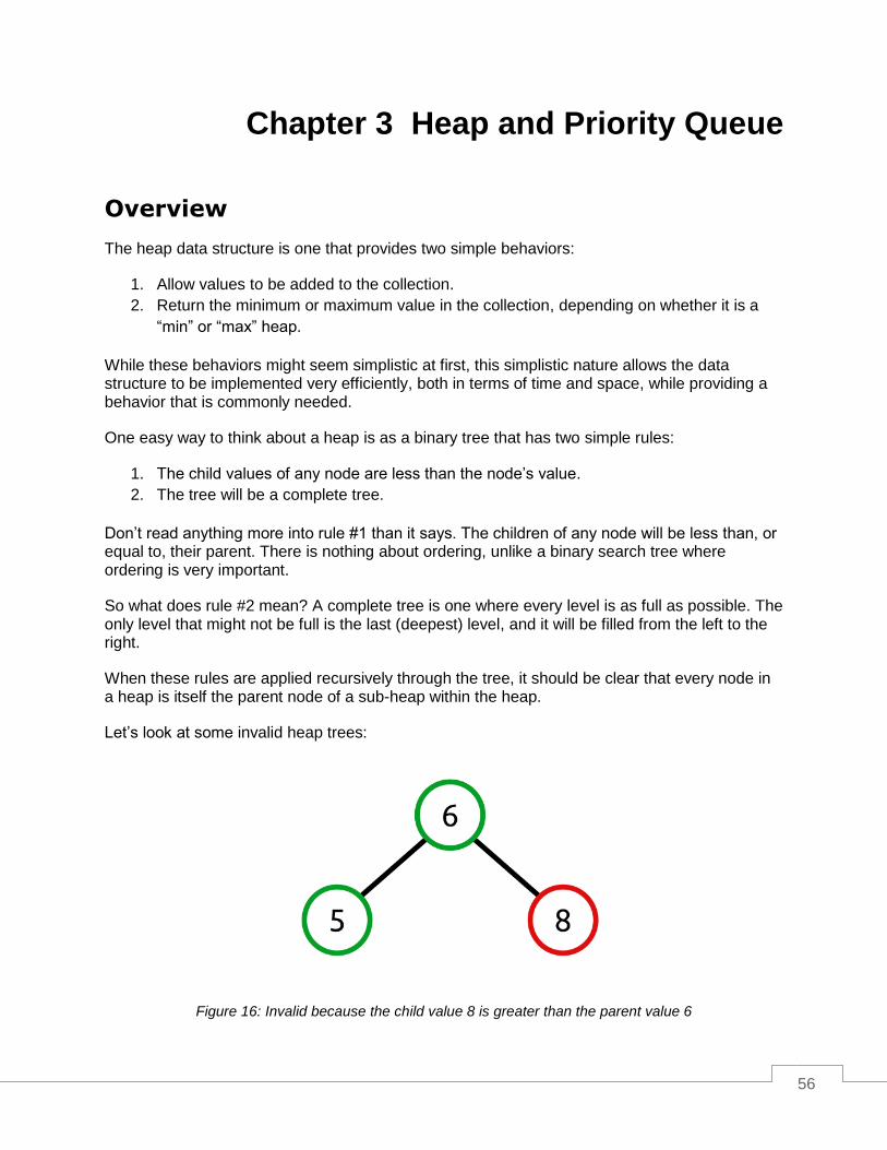
Let’s look at some invalid heap trees:

Figure 16: Invalid because the child value 8 is greater than the parent value 6

57

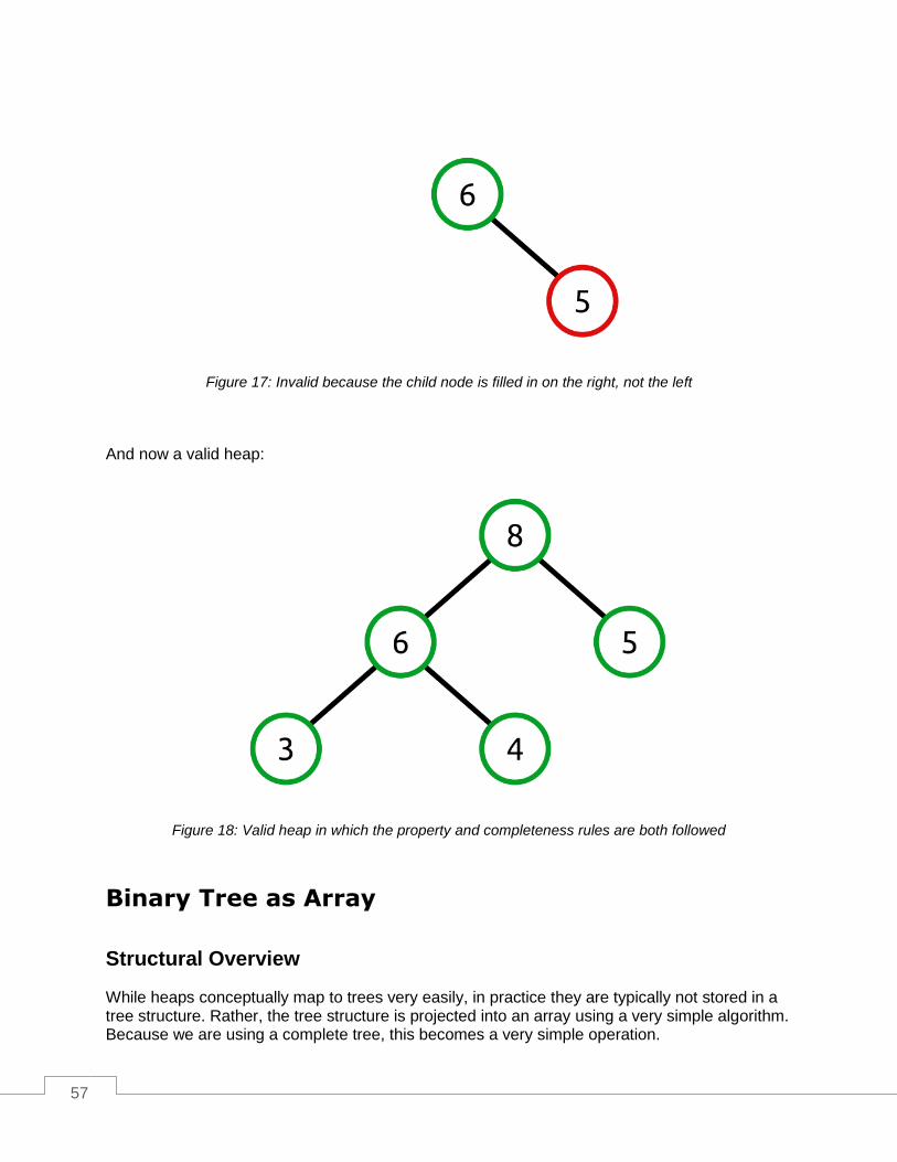
Figure 17: Invalid because the child node is filled in on the right, not the left

And now a valid heap:

Figure 18: Valid heap in which the property and completeness rules are both followed

Binary Tree as Array

Structural Overview

While heaps conceptually map to trees very easily, in practice they are typically not stored in a tree structure. Rather, the tree structure is projected into an array using a very simple algorithm. Because we are using a complete tree, this becomes a very simple operation.

58

Let’s start by looking at a tree whose nodes are colored based on what level they are in within the tree.

Figure 19: Tree with colors based on level

This is a complete tree with seven nodes across three levels. We fit this level-by-level into an array like so:

Figure 20: The binary tree projected into the array

The root node (level 1) is in the first array index. Its children (the next level) follow. Their children follow. This pattern continues for every level of the tree. Notice there is even an unused array index at the end of the array. This will become important when we want to add more data to the heap.

Let’s look at a concrete example where this valid heap maps into an array.

59

Figure 21: A valid heap as a binary tree

Figure 22: The valid heap tree mapped into an array

Navigating the Array like a Tree

One of the nice benefits of trees is that they are very easy to navigate both in an iterative and recursive fashion. Moving up or down the tree is as simple as navigating to the child nodes or back up to the parent.

If we are going to efficiently use an array to contain our tree data, we need to have equally efficient mechanisms to determine two facts:

1. Given an index, what indexes represent its children?

2. Given an index, what index represents its parent?

It turns out this is very simple.

The children of any index are:

Left child index = 2 × <current index> + 1

Right child index = 2 × <current index> + 2

60

Let’s prove that works. Recall that the root node is stored in index 0. Using the formula, we see that its left child can be found at index 1 (using the formula 2 × 0 + 1) and its right child at index 2 (2 × 0 + 2).

Finding the parent of any node is simply the inverse of that function:

Parent = (index - 1) / 2

Technically, it is floor((index - 1) / 2). However, C# handles the integer truncation for us.

The Key Point

The critical point to take away from this section is this: the largest value in the heap is always the first item in the array.

Heap Class

The heap class we will be implementing is a max heap, meaning that it returns the maximum value very efficiently. The class is very straightforward. It has a method to add a new value, remove the maximum value, peek at the maximum value, clear the collection, and get the current count of items in the heap.

The heap requires that its generic type argument implements the IComparable<T> interface

and has two fields: the backing array and the current count of items in the heap. Two utility methods, Swap and Parent, are shown here as well.

Notice that there are no methods for enumeration or performing other look-up operations such as determining if the heap contains a specific value or directly indexing into the heap. While those methods would not be terribly difficult to add, they are in conflict with what a heap is. A heap is an opaque container that returns the minimum or maximum value.

public class Heap<T> where T: IComparable<T> { T[] _items; int _count; const int DEFAULT_LENGTH = 100; public Heap() : this(DEFAULT_LENGTH) { } public Heap(int length) { _items = new T[length]; _count = 0; } public void Add(T value);

61

Add

Behavior Adds the provided value to the heap.


Adding a value to the heap has two steps:

1. Add the value to the end of the backing array (growing if necessary).

2. Swap the value with its parent until the heap property is satisfied.

For example, let’s look at our valid heap from before:

public T Peek(); public T RemoveMax(); public int Count { get; } public void Clear(); private int Parent(int index) { return (index - 1) / 2; } private void Swap(int left, int right) { T temp = _items[left]; _items[left] = _items[right]; _items[right] = temp; } }

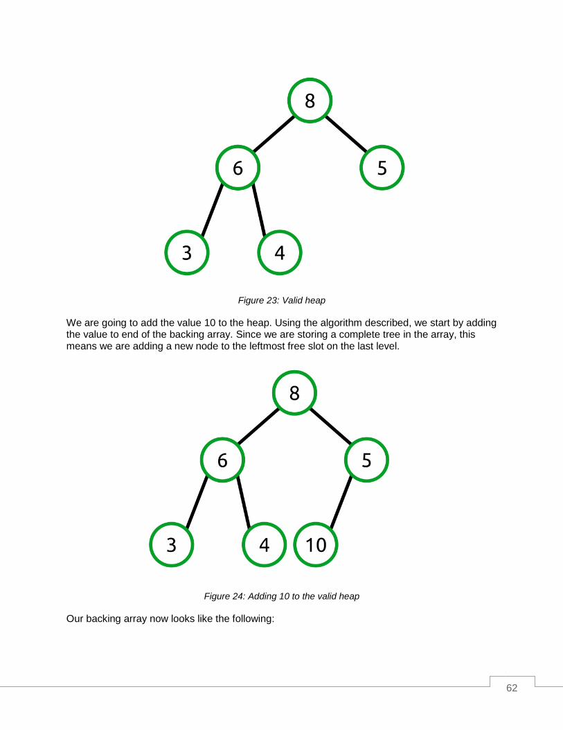
62

Figure 23: Valid heap

We are going to add the value 10 to the heap. Using the algorithm described, we start by adding the value to end of the backing array. Since we are storing a complete tree in the array, this means we are adding a new node to the leftmost free slot on the last level.

Figure 24: Adding 10 to the valid heap

Our backing array now looks like the following:

63

You should notice that this violates the heap property that requires each node’s children to be less than or equal to the parent node’s value. In this case, the value 5 has a child whose value is 10. To fix this, we need to swap the nodes like so:

Figure 25: Swapping the 10 and 5 nodes

Our backing array now looks like this:

We have now fixed the relationship between 10 and 5, but the parent node of 10 is 8, and that violates the heap property, so we need to swap those as well.

[8, 6, 5, 3, 4, 10]

[8, 6, 10, 3, 4, 5]

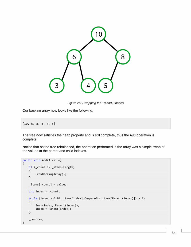
64

Figure 26: Swapping the 10 and 8 nodes

Our backing array now looks like the following:

The tree now satisfies the heap property and is still complete, thus the Add operation is

complete.

Notice that as the tree rebalanced, the operation performed in the array was a simple swap of the values at the parent and child indexes.

[10, 6, 8, 3, 4, 5]

public void Add(T value) { if (_count >= _items.Length) { GrowBackingArray(); } _items[_count] = value; int index = _count; while (index > 0 && _items[index].CompareTo(_items[Parent(index)]) > 0) { Swap(index, Parent(index)); index = Parent(index); } _count++; }

65

RemoveMax

Behavior Removes and returns the largest value in the heap. An exception is thrown if the heap is empty.


RemoveMax works similar to Add, but in the opposite direction. Where Add starts at the bottom of

the tree (or the end of the array) and works the value upward to its appropriate location, RemoveMax starts by storing away the largest value in the heap which is in array index 0. This is

the value that will be returned to the caller.

Since that value is being removed, the array index 0 is now free. To ensure that our array does not have any gaps, we need to move something into it. What we do is grab the last item in the array and move it forward to index 0. In a tree view it would look like this:

Figure 27: Moving the last array item to index 0

private void GrowBackingArray() { T[] newItems = new T[_items.Length * 2]; for (int i = 0; i < _items.Length; i++) { newItems[i] = _items[i]; } _items = newItems; }

66

Our backing array changes like so:

As with Add, the tree is not in a valid state. However, unlike Add, the bad node is the root (array

index 0) rather than the last node.

What we need to do is swap the smaller parent node with its children until the heap property is satisfied. This just leaves the question: what child do we swap with? The answer is that we always swap with the largest child. Consider what would happen if we swapped with the lesser child. The tree would switch from one invalid state to another. For example:

Figure 28: Swapping with the lesser value does not create a valid heap

We haven’t solved the problem! Instead, we need to swap with the larger of the two children like so:

[10, 6, 8, 3, 4, 5] => [5, 6, 8, 3, 4]

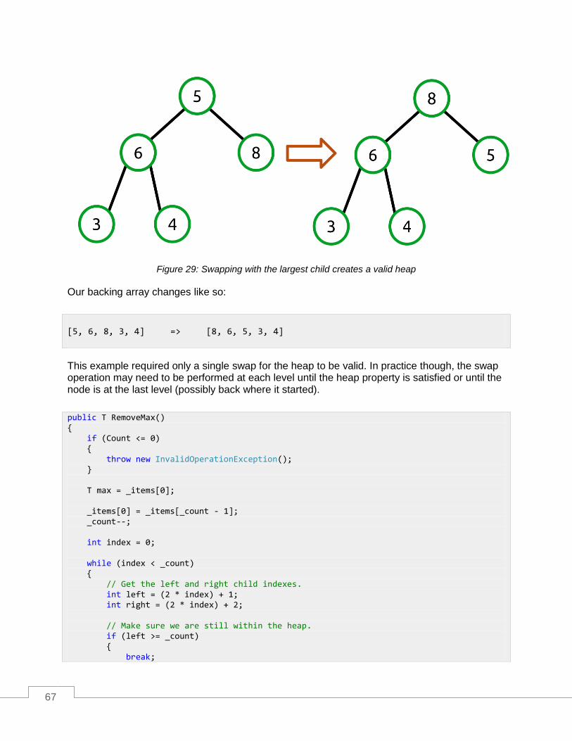
67

Figure 29: Swapping with the largest child creates a valid heap

Our backing array changes like so:

This example required only a single swap for the heap to be valid. In practice though, the swap operation may need to be performed at each level until the heap property is satisfied or until the node is at the last level (possibly back where it started).

[5, 6, 8, 3, 4] => [8, 6, 5, 3, 4]

public T RemoveMax() { if (Count <= 0) { throw new InvalidOperationException(); } T max = _items[0]; _items[0] = _items[_count - 1]; _count--; int index = 0; while (index < _count) { // Get the left and right child indexes. int left = (2 * index) + 1; int right = (2 * index) + 2; // Make sure we are still within the heap. if (left >= _count) { break;

68

} // To avoid having to swap twice, we swap with the largest value. // E.g., // 5 // 6 8 // // If we swapped with 6 first we'd have // // 6 // 5 8 // // and we'd require another swap to get the desired tree. // // 8 // 6 5 // // So we find the largest child and just do the right thing at the start. int maxChildIndex = IndexOfMaxChild(left, right); if (_items[index].CompareTo(_items[maxChildIndex]) > 0) { // The current item is larger than its children (heap property is satisfied). break; } Swap(index, maxChildIndex); index = maxChildIndex; } return max; } private int IndexOfMaxChild(int left, int right) { // Find the index of the child with the largest value. int maxChildIndex = -1; if (right >= _count) { // No right child. maxChildIndex = left; } else { if (_items[left].CompareTo(_items[right]) > 0) { maxChildIndex = left; } else { maxChildIndex = right; } } return maxChildIndex; }

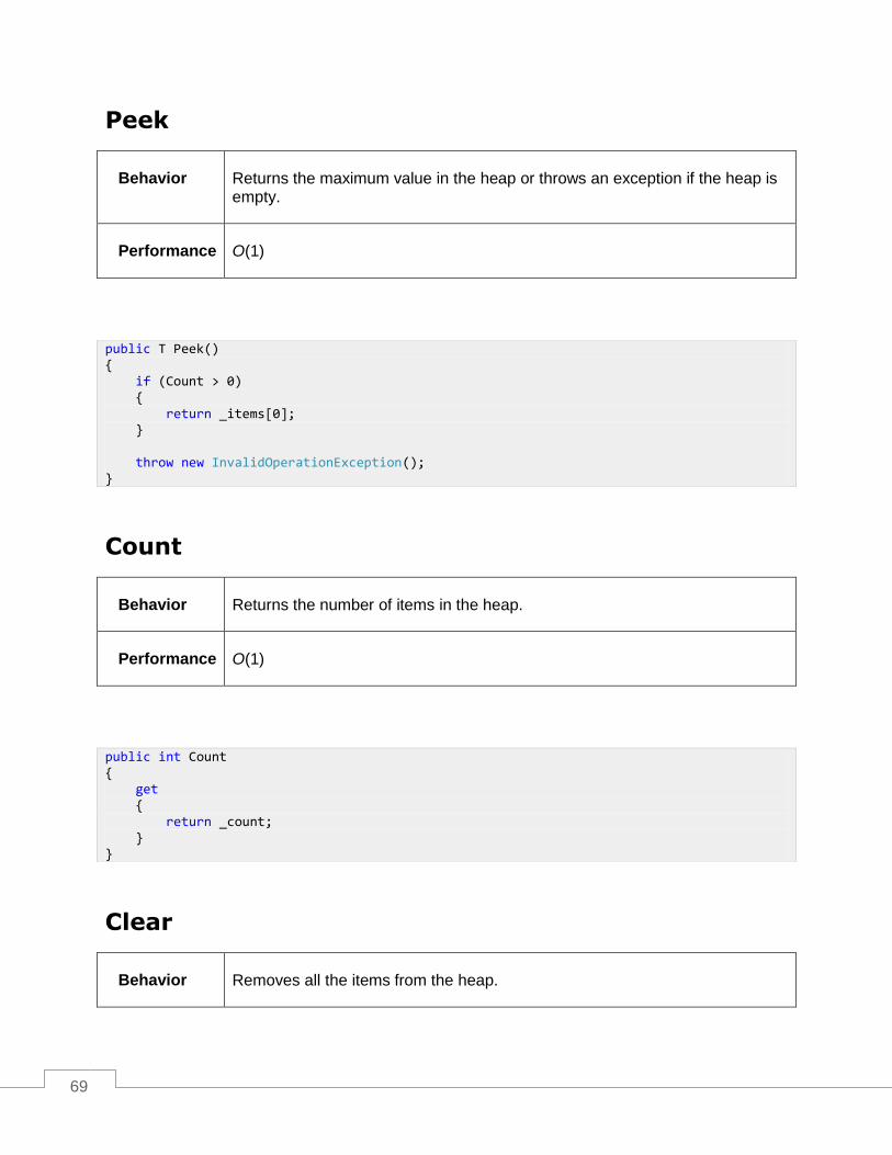
69

Peek

Behavior Returns the maximum value in the heap or throws an exception if the heap is empty.

Performance O(1)

Count

Behavior Returns the number of items in the heap.

Performance O(1)

Clear

Behavior Removes all the items from the heap.

public T Peek() { if (Count > 0) { return _items[0]; } throw new InvalidOperationException(); }

public int Count { get { return _count; } }

70

Performance O(1)

Clear sets the count to 0 and allocates a new default-length array. The array allocation is done

to ensure that the garbage collector has a chance to free any objects that were referenced by the heap before Clear was called.

Priority Queue

A priority queue is a cross between a queue and heap. It looks and feels like a queue—items can be enqueued and dequeued. However, the value that is returned is the highest priority item.

Priority queues are commonly used in scenarios where many items are being processed, some of which are more important than others.

Network routing is an example I think we can all relate to. Not all network traffic is equal. Some data, such as real-time voice communications, requires a high quality of service while other data, such as background file transfers for a network backup program, require a lower quality of service.

If my computer is sending packets for both a VoIP phone connection and transferring pictures of my vacation to Facebook, it is very likely that I want the voice connection to take priority over the picture transfer. I probably won’t notice if the picture transfer takes a little longer, but you can be sure I will notice if my voice call quality is poor.

In this example, the network stack might provide a mechanism that allows the network traffic to declare some priority property for itself which determines how time-sensitive the data is. The network stack might use a priority queue internally to make this happen. This is obviously a trivialization of a complex topic, but the point should be clear: some data sets are more important than others.

Priority Queue Class

The priority queue class is a very thin wrapper over a heap. All it really does is wrap the Add and

RemoveMax methods with Enqueue and Dequeue, respectively.

public void Clear() { _count = 0; _items = new T[DEFAULT_LENGTH]; }

public class PriorityQueue<T> where T: IComparable<T> { Heap<T> _heap = new Heap<T>();

71

Usage Example

This example creates a simple application where messages are queued with these:

A priority from 0 (lowest) to 3 (highest).

The age of the message.

The message itself (a string).

A priority queue is used to ensure that messages are processed in order of priority. Multiple messages within a given priority are processed from oldest to newest.

The Data class has the three properties noted in the previous list, a ToString method to print

the properties in a structured manner, and an IComparable<Data>.CompareTo method that

performs a comparison by Priority and Age.

public void Enqueue(T value) { _heap.Add(value); } public T Dequeue() { return _heap.RemoveMax(); } public void Clear() { _heap.Clear(); } public int Count { get { return _heap.Count; } } }

class Data : IComparable<Data> { readonly DateTime _creationTime; public Data(string message, int priority) { _creationTime = DateTime.UtcNow; Message = message; Priority = priority; } public string Message { get; private set; }

72

Next, there is a simple class that adds 1000 random-priority messages to the queue with a short, 0–3 millisecond delay between messages to ensure that ordering can be demonstrated both by priority and time.

The application then prints out the messages in priority and age order to demonstrate how the priority queue can be used.

public int Priority { get; private set; } public TimeSpan Age { get { return DateTime.UtcNow.Subtract(_creationTime); } } public int CompareTo(Data other) { int pri = Priority.CompareTo(other.Priority); if (pri == 0) { pri = Age.CompareTo(other.Age); } return pri; } public override string ToString() { return string.Format("[{0} : {1}] {2}", Priority, Age.Milliseconds, Message); } }

static void PriorityQueueSample() { PriorityQueue<Data> queue = new PriorityQueue<Data>(); queue = new PriorityQueue<Data>(); Random rng = new Random(); for (int i = 0; i < 1000; i++) { int priority = rng.Next() % 3; queue.Enqueue(new Data(string.Format("This is message: {0}", i), priority)); Thread.Sleep(priority); } while (queue.Count > 0) { Console.WriteLine(queue.Dequeue().ToString()); } }

73

Chapter 4 AVL Tree

Balanced Tree Overview

An AVL tree is a self-balancing binary search tree. It is named after its inventors, G. M. Adelson-Velskii and E. M. Landis, who first described the structure and associated algorithms in 1962. Like the binary search tree introduced in the first book of this series, an AVL tree maintains these three simple rules:

Each node in the tree will have at most two child nodes (the “left” and “right” children).

Values smaller than the current node will go to the left.

Values larger than or equal to the current node will go on the right.

In addition, the AVL tree adds a new rule:

The height of the left and right nodes will never differ by more than 1.

What is Node Height?

The distance between any two related nodes can be measured.

Figure 30: Node Height

The previous figure shows a binary tree with lines indicating the levels of each set of nodes. The root node, 6, has no parent so it is at level 1. Nodes 4 and 8 are sibling nodes that are both at level 2. Nodes 3 and 5 are at level 3.

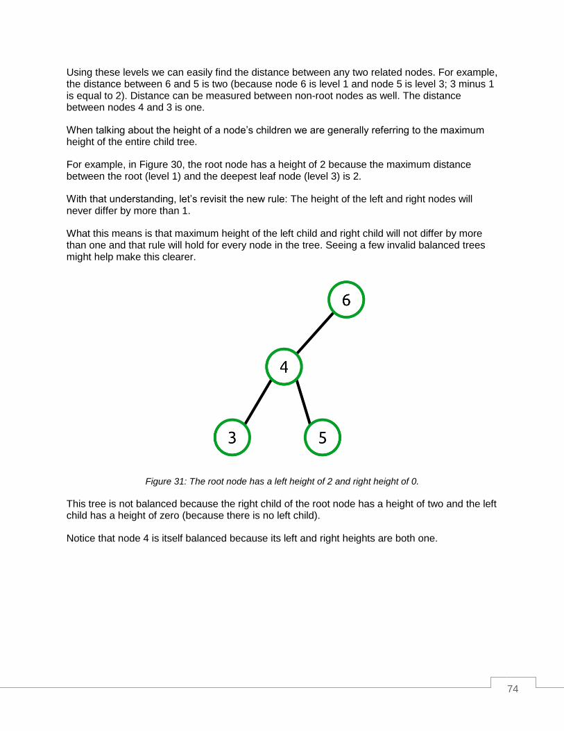
74

Using these levels we can easily find the distance between any two related nodes. For example, the distance between 6 and 5 is two (because node 6 is level 1 and node 5 is level 3; 3 minus 1 is equal to 2). Distance can be measured between non-root nodes as well. The distance between nodes 4 and 3 is one.

When talking about the height of a node’s children we are generally referring to the maximum height of the entire child tree.

For example, in Figure 30, the root node has a height of 2 because the maximum distance between the root (level 1) and the deepest leaf node (level 3) is 2.

With that understanding, let’s revisit the new rule: The height of the left and right nodes will never differ by more than 1.

What this means is that maximum height of the left child and right child will not differ by more than one and that rule will hold for every node in the tree. Seeing a few invalid balanced trees might help make this clearer.

Figure 31: The root node has a left height of 2 and right height of 0.

This tree is not balanced because the right child of the root node has a height of two and the left child has a height of zero (because there is no left child).

Notice that node 4 is itself balanced because its left and right heights are both one.

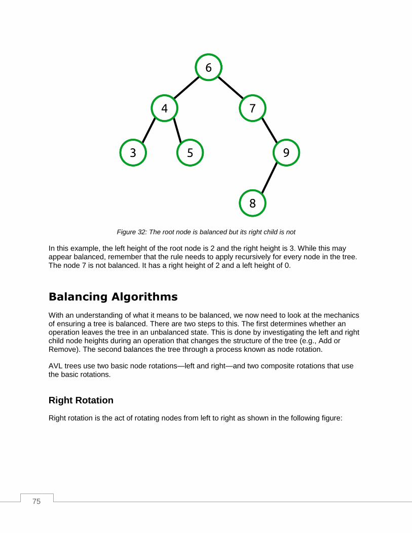
75

Figure 32: The root node is balanced but its right child is not

In this example, the left height of the root node is 2 and the right height is 3. While this may appear balanced, remember that the rule needs to apply recursively for every node in the tree. The node 7 is not balanced. It has a right height of 2 and a left height of 0.

Balancing Algorithms

With an understanding of what it means to be balanced, we now need to look at the mechanics of ensuring a tree is balanced. There are two steps to this. The first determines whether an operation leaves the tree in an unbalanced state. This is done by investigating the left and right child node heights during an operation that changes the structure of the tree (e.g., Add or Remove). The second balances the tree through a process known as node rotation.

AVL trees use two basic node rotations—left and right—and two composite rotations that use the basic rotations.

Right Rotation

Right rotation is the act of rotating nodes from left to right as shown in the following figure:

76

Figure 33: Right rotation moves the root’s left child into the root position

Figure 34: Right rotation moves the right child of the root’s left child to the left child of the old root

The algorithm for right rotation has three steps. These steps are all from the perspective of the original root node (B).

1. Replace the current root with its immediate left child (this becomes the new root).

The B node moves its left child (A) into its place.

2. Move the new root’s right child to the old root’s left child.

This changes B > C to D > C.

3. Assign the old root (D) to be the new root’s (B) right child.

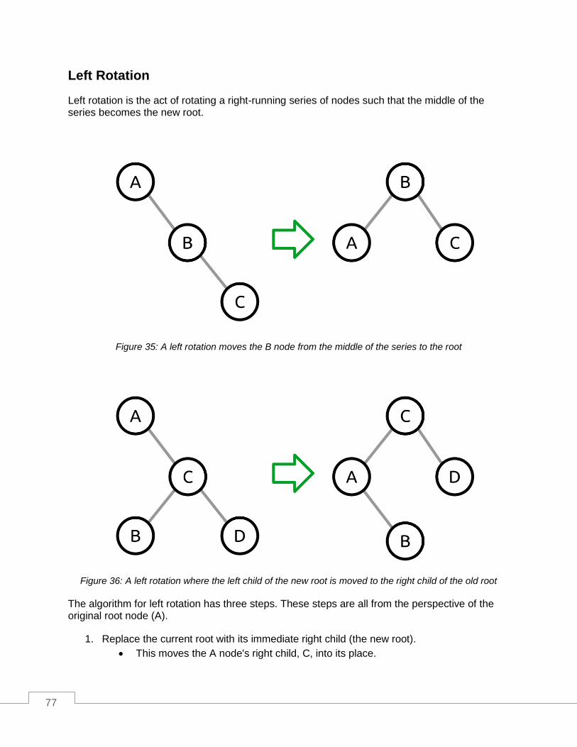
77

Left Rotation

Left rotation is the act of rotating a right-running series of nodes such that the middle of the series becomes the new root.

Figure 35: A left rotation moves the B node from the middle of the series to the root

Figure 36: A left rotation where the left child of the new root is moved to the right child of the old root

The algorithm for left rotation has three steps. These steps are all from the perspective of the original root node (A).

1. Replace the current root with its immediate right child (the new root).

This moves the A node's right child, C, into its place.

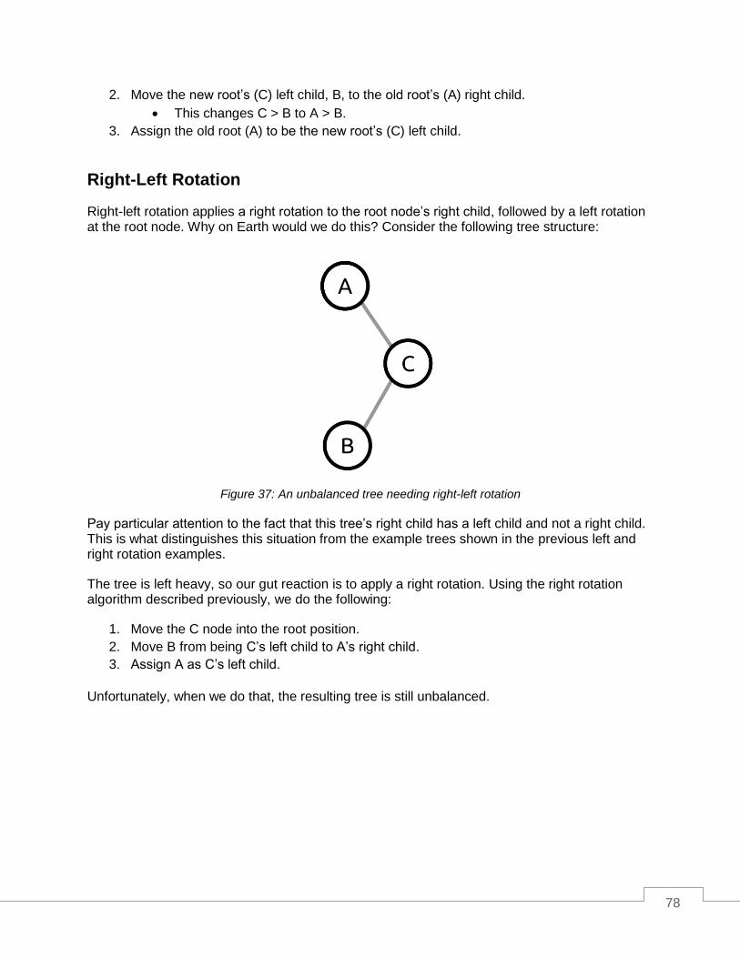
78

2. Move the new root’s (C) left child, B, to the old root’s (A) right child.

This changes C > B to A > B.

3. Assign the old root (A) to be the new root’s (C) left child.

Right-Left Rotation

Right-left rotation applies a right rotation to the root node’s right child, followed by a left rotation at the root node. Why on Earth would we do this? Consider the following tree structure:

Figure 37: An unbalanced tree needing right-left rotation

Pay particular attention to the fact that this tree’s right child has a left child and not a right child. This is what distinguishes this situation from the example trees shown in the previous left and right rotation examples.

The tree is left heavy, so our gut reaction is to apply a right rotation. Using the right rotation algorithm described previously, we do the following:

1. Move the C node into the root position.

2. Move B from being C’s left child to A’s right child.

3. Assign A as C’s left child.

Unfortunately, when we do that, the resulting tree is still unbalanced.

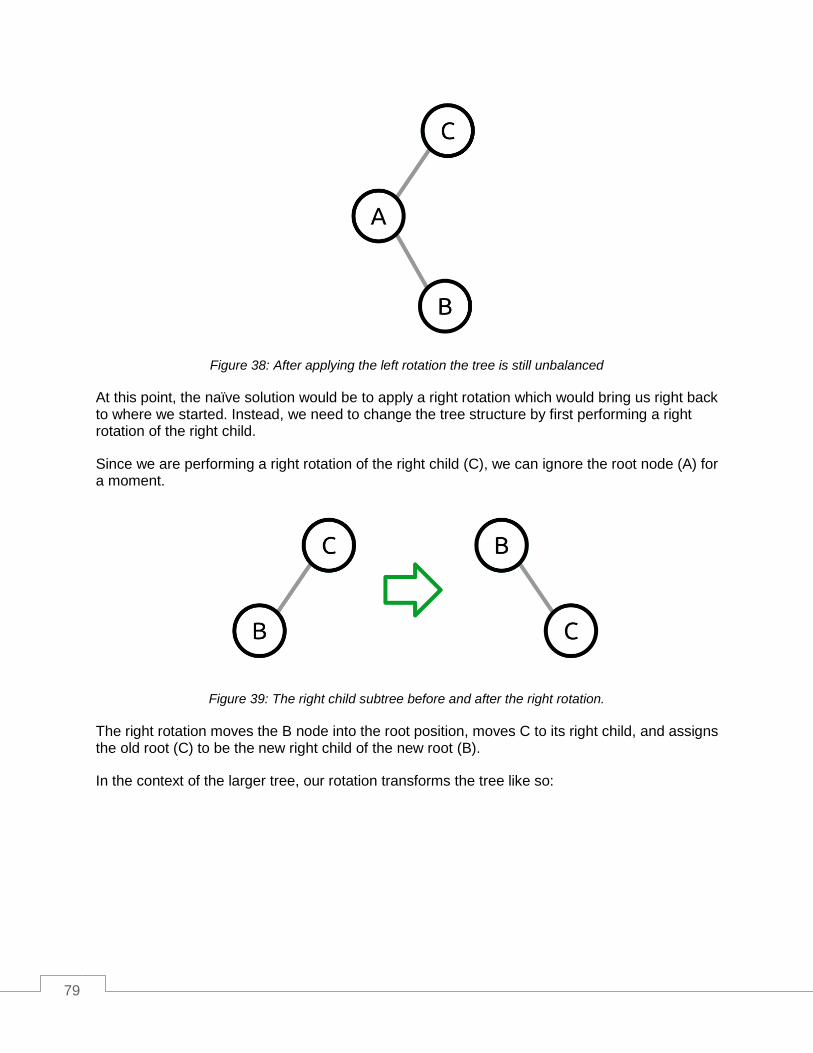
79

Figure 38: After applying the left rotation the tree is still unbalanced

At this point, the naïve solution would be to apply a right rotation which would bring us right back to where we started. Instead, we need to change the tree structure by first performing a right rotation of the right child.

Since we are performing a right rotation of the right child (C), we can ignore the root node (A) for a moment.

Figure 39: The right child subtree before and after the right rotation.

The right rotation moves the B node into the root position, moves C to its right child, and assigns the old root (C) to be the new right child of the new root (B).

In the context of the larger tree, our rotation transforms the tree like so:

80

Figure 40: A right rotation performed on the right child

The resulting tree (A > B > C) is something we know how to rotate using the left rotation algorithm. So the entire process looks like the following:

Figure 41: The entire right-left rotation process

Left-Right Rotation

Left-right rotation is simply the opposite of right-left rotation. We start with an unbalanced tree where the root node has a left child which has a right child but no left child. Once we have identified this situation, the solution is to apply a left rotation to the left child and then apply a right rotation to the root. The entire left-right rotation process is shown in the following figure:

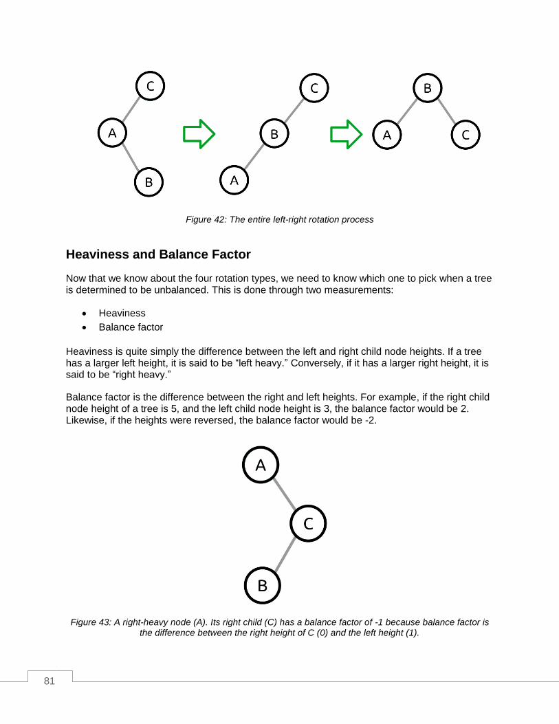
81

Figure 42: The entire left-right rotation process

Heaviness and Balance Factor

Now that we know about the four rotation types, we need to know which one to pick when a tree is determined to be unbalanced. This is done through two measurements:

Heaviness

Balance factor

Heaviness is quite simply the difference between the left and right child node heights. If a tree has a larger left height, it is said to be “left heavy.” Conversely, if it has a larger right height, it is said to be “right heavy.”

Balance factor is the difference between the right and left heights. For example, if the right child node height of a tree is 5, and the left child node height is 3, the balance factor would be 2. Likewise, if the heights were reversed, the balance factor would be -2.

Figure 43: A right-heavy node (A). Its right child (C) has a balance factor of -1 because balance factor is the difference between the right height of C (0) and the left height (1).

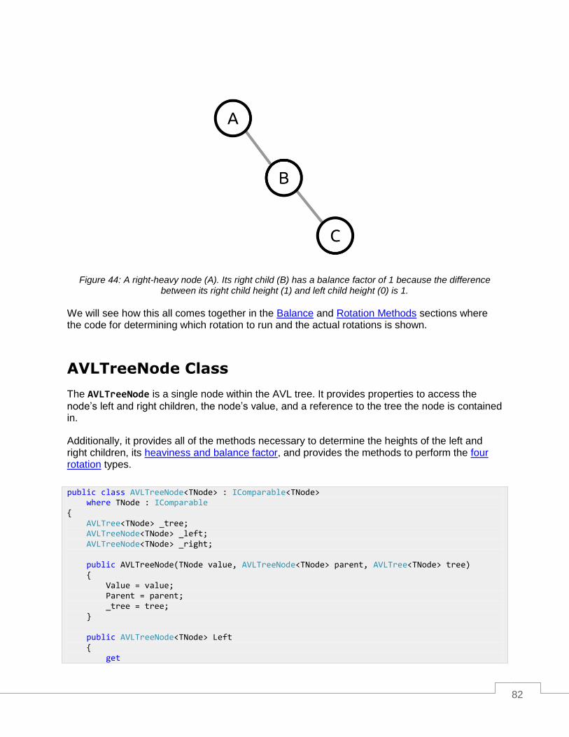
82

Figure 44: A right-heavy node (A). Its right child (B) has a balance factor of 1 because the difference between its right child height (1) and left child height (0) is 1.

We will see how this all comes together in the Balance and Rotation Methods sections where the code for determining which rotation to run and the actual rotations is shown.

AVLTreeNode Class

The AVLTreeNode is a single node within the AVL tree. It provides properties to access the

node’s left and right children, the node’s value, and a reference to the tree the node is contained in.

Additionally, it provides all of the methods necessary to determine the heights of the left and right children, its heaviness and balance factor, and provides the methods to perform the four rotation types.

public class AVLTreeNode<TNode> : IComparable<TNode> where TNode : IComparable { AVLTree<TNode> _tree; AVLTreeNode<TNode> _left; AVLTreeNode<TNode> _right; public AVLTreeNode(TNode value, AVLTreeNode<TNode> parent, AVLTree<TNode> tree) { Value = value; Parent = parent; _tree = tree; } public AVLTreeNode<TNode> Left { get

83

Balance

The balance algorithm determines if a rotation is needed, and if so, what rotation needs to be performed. It does this by first checking to see if the tree is unbalanced.

{ return _left; } internal set { _left = value; if (_left != null) { _left.Parent = this; } } } public AVLTreeNode<TNode> Right { get { return _right; } internal set { _right = value; if (_right != null) { _right.Parent = this; } } } public AVLTreeNode<TNode> Parent { get; internal set; } public TNode Value { get; private set; } /// <summary> /// Compares the current node to the provided value. /// </summary> /// <param name="other">The node value to compare to.</param> /// <returns>1 if the instance value is greater than the provided value, -1 if less, or 0 if equal.</returns> public int CompareTo(TNode other) { return Value.CompareTo(other); } // The rest of the code for the AVLTreeNode class is // in the subsequent sections of this chapter. }

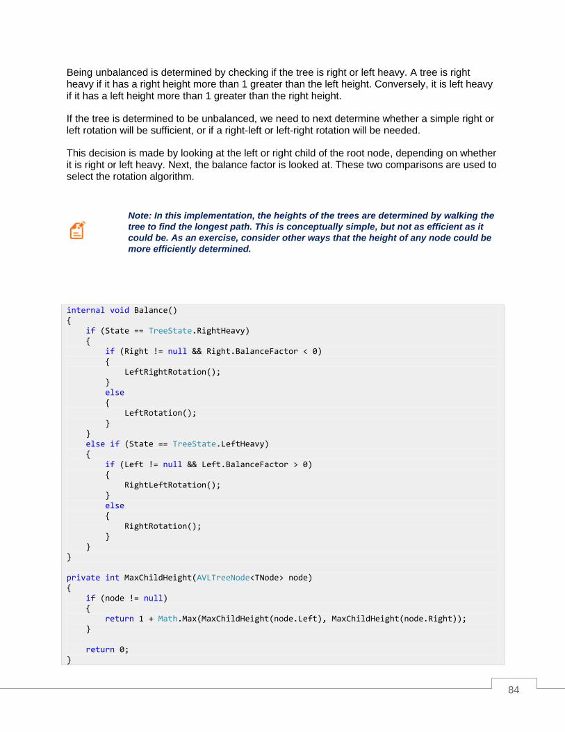
84

Being unbalanced is determined by checking if the tree is right or left heavy. A tree is right heavy if it has a right height more than 1 greater than the left height. Conversely, it is left heavy if it has a left height more than 1 greater than the right height.

If the tree is determined to be unbalanced, we need to next determine whether a simple right or left rotation will be sufficient, or if a right-left or left-right rotation will be needed.

This decision is made by looking at the left or right child of the root node, depending on whether it is right or left heavy. Next, the balance factor is looked at. These two comparisons are used to select the rotation algorithm.

Note: In this implementation, the heights of the trees are determined by walking the

tree to find the longest path. This is conceptually simple, but not as efficient as it

could be. As an exercise, consider other ways that the height of any node could be

more efficiently determined.

internal void Balance() { if (State == TreeState.RightHeavy) { if (Right != null && Right.BalanceFactor < 0) { LeftRightRotation(); } else { LeftRotation(); } } else if (State == TreeState.LeftHeavy) { if (Left != null && Left.BalanceFactor > 0) { RightLeftRotation(); } else { RightRotation(); } } } private int MaxChildHeight(AVLTreeNode<TNode> node) { if (node != null) { return 1 + Math.Max(MaxChildHeight(node.Left), MaxChildHeight(node.Right)); } return 0; }

85

private int LeftHeight { get { return MaxChildHeight(Left); } } private int RightHeight { get { return MaxChildHeight(Right); } } private TreeState State { get { if (LeftHeight - RightHeight > 1) { return TreeState.LeftHeavy; } if (RightHeight - LeftHeight > 1) { return TreeState.RightHeavy; } return TreeState.Balanced; } } private int BalanceFactor { get { return RightHeight - LeftHeight; } } enum TreeState { Balanced, LeftHeavy, RightHeavy, }

86

Rotation Methods

The rotations are implementations of the algorithms discussed in the Balancing Algorithms section. The ReplaceRoot method handles the mechanics of moving the child node into the

root node’s position. The parent node of the original root needs to be updated to point to the new root node. If there is no parent node, the containing tree needs to be made aware of the new tree root node.

private void LeftRotation() { // a // \ // b // \ // c // // becomes // b // / \ // a c AVLTreeNode<TNode> newRoot = Right; // Replace the current root with the new root. ReplaceRoot(newRoot); // Take ownership of right's left child as right (now parent). Right = newRoot.Left; // The new root takes this as its left. newRoot.Left = this; } private void RightRotation() { // c (this) // / // b // / // a // // becomes // b // / \ // a c AVLTreeNode<TNode> newRoot = Left; // Replace the current root with the new root. ReplaceRoot(newRoot); // Take ownership of left's right child as left (now parent). Left = newRoot.Right; // The new root takes this as its right. newRoot.Right = this;

87

AVLTree Class

The AVL tree class provides the basic collection methods to add, remove, enumerate, and check if a value exists within the tree. Additionally, it provides the ability to clear the tree and get the count of nodes in the tree.

} private void LeftRightRotation() { Right.RightRotation(); LeftRotation(); } private void RightLeftRotation() { Left.LeftRotation(); RightRotation(); } private void ReplaceRoot(AVLTreeNode<TNode> newRoot) { if (this.Parent != null) { if (this.Parent.Left == this) { this.Parent.Left = newRoot; } else if (this.Parent.Right == this) { this.Parent.Right = newRoot; } } else { _tree.Head = newRoot; } newRoot.Parent = this.Parent; this.Parent = newRoot; }

public class AVLTree<T> : IEnumerable<T> where T : IComparable { public AVLTreeNode<T> Head { get; internal set; } public void Add(T value); public bool Contains(T value); public bool Remove(T value);

88

Add

Behavior Adds the specific value to the tree, ensuring that the tree is in a balanced state when the method completes.


The AVL tree Add operation is nearly identical to the binary search tree add operation. It walks

the tree using the rules described previously in this chapter. Once the appropriate node location is found, the node is inserted into the tree. Since the tree might now be unbalanced, the node performs the balance operation to ensure the tree is balanced when the Add method returns.

public IEnumerator<T> GetEnumerator(); System.Collections.IEnumerator System.Collections.IEnumerable.GetEnumerator(); public void Clear(); public int Count { get; private set; } }

public void Add(T value) { // Case 1: The tree is empty--allocate the head. if (Head == null) { Head = new AVLTreeNode<T>(value, null, this); } // Case 2: The tree is not empty--find the right location to insert. else { AddTo(Head, value); } Count++; } // Recursive add algorithm. private void AddTo(AVLTreeNode<T> node, T value) { // Case 1: Value is less than the current node value. if (value.CompareTo(node.Value) < 0) { // If there is no left child, make this the new left. if (node.Left == null) { node.Left = new AVLTreeNode<T>(value, node, this); } else { // Else, add it to the left node.

89

Contains

Behavior Returns true if the specific value is contained within the tree. Otherwise it

returns false.


A traditional binary search tree has O(n) worst-case complexity because a pathologically unbalanced tree is basically a linked list. Because an AVL tree is balanced, we have a guaranteed complexity of O(log n).

AddTo(node.Left, value); } } // Case 2: Value is equal to or greater than the current value. else { // If there is no right, add it to the right. if (node.Right == null) { node.Right = new AVLTreeNode<T>(value, node, this); } else { // Else, add it to the right node. AddTo(node.Right, value); } } node.Balance(); }

public bool Contains(T value) { return Find(value) != null; } /// <summary> /// Finds and returns the first node containing the specified value. If the value /// is not found, it returns null. It also returns the parent of the found node (or null) /// which is used in Remove. /// </summary> /// <param name="value">The value to search for.</param> /// <param name="parent">The parent of the found node (or null).</param> /// <returns>The found node (or null).</returns> private AVLTreeNode<T> Find(T value) { // Now, try to find data in the tree. AVLTreeNode<T> current = Head;

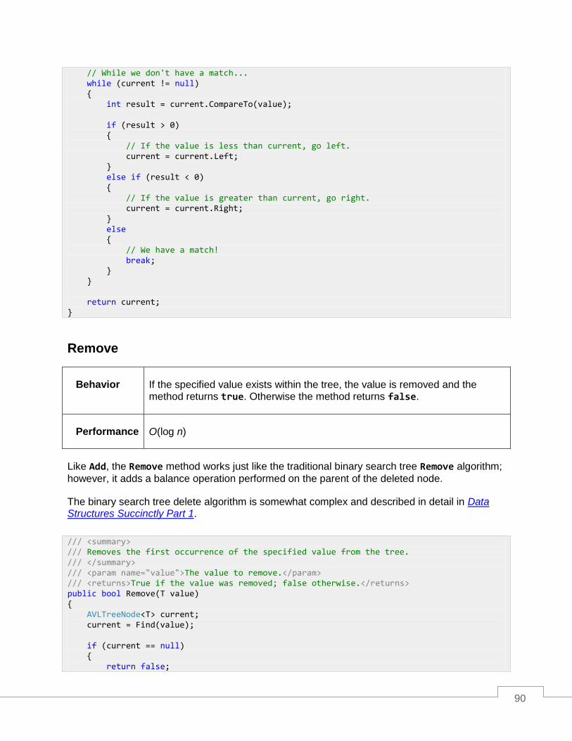
90

Remove

Behavior If the specified value exists within the tree, the value is removed and the method returns true. Otherwise the method returns false.


Like Add, the Remove method works just like the traditional binary search tree Remove algorithm;

however, it adds a balance operation performed on the parent of the deleted node.

The binary search tree delete algorithm is somewhat complex and described in detail in Data Structures Succinctly Part 1.

// While we don't have a match... while (current != null) { int result = current.CompareTo(value); if (result > 0) { // If the value is less than current, go left. current = current.Left; } else if (result < 0) { // If the value is greater than current, go right. current = current.Right; } else { // We have a match! break; } } return current; }

/// <summary> /// Removes the first occurrence of the specified value from the tree. /// </summary> /// <param name="value">The value to remove.</param> /// <returns>True if the value was removed; false otherwise.</returns> public bool Remove(T value) { AVLTreeNode<T> current; current = Find(value); if (current == null) { return false;

http://www.syncfusion.com/resources/techportal/ebooks/datastructurespart1

http://www.syncfusion.com/resources/techportal/ebooks/datastructurespart1

91

} AVLTreeNode<T> treeToBalance = current.Parent; Count--; // Case 1: If current has no right child, then current's left replaces current. if (current.Right == null) { if (current.Parent == null) { Head = current.Left; if (Head != null) { Head.Parent = null; } } else { int result = current.Parent.CompareTo(current.Value); if (result > 0) { // If the parent value is greater than the current value, // make the current left child a left child of parent. current.Parent.Left = current.Left; } else if (result < 0) { // If the parent value is less than the current value, // make the current left child a right child of parent. current.Parent.Right = current.Left; } } } // Case 2: If current's right child has no left child, then current's right child // replaces current. else if (current.Right.Left == null) { current.Right.Left = current.Left; if (current.Parent == null) { Head = current.Right; if (Head != null) { Head.Parent = null; } } else { int result = current.Parent.CompareTo(current.Value); if (result > 0) { // If the parent value is greater than the current value, // make the current right child a left child of parent. current.Parent.Left = current.Right; }

92

else if (result < 0) { // If the parent value is less than the current value, // make the current right child a right child of parent. current.Parent.Right = current.Right; } } } // Case 3: If current's right child has a left child, replace current with current's // right child's leftmost child. else { // Find the right's leftmost child. AVLTreeNode<T> leftmost = current.Right.Left; while (leftmost.Left != null) { leftmost = leftmost.Left; } // The parent's left subtree becomes the leftmost's right subtree. leftmost.Parent.Left = leftmost.Right; // Assign leftmost's left and right to current's left and right children. leftmost.Left = current.Left; leftmost.Right = current.Right; if (current.Parent == null) { Head = leftmost; if (Head != null) { Head.Parent = null; } } else { int result = current.Parent.CompareTo(current.Value); if (result > 0) { // If the parent value is greater than the current value, // make leftmost the parent's left child. current.Parent.Left = leftmost; } else if (result < 0) { // If the parent value is less than the current value, // make leftmost the parent's right child. current.Parent.Right = leftmost; } } } if (treeToBalance != null) { treeToBalance.Balance(); }

93

GetEnumerator

Behavior Returns an enumerator that performs an inorder traversal of the AVL tree.

Performance O(1) to return the enumerator. O(n) for the caller to enumerate each node.

The inorder (smallest to largest value) traversal algorithm is described in more detail in book one of this series. The implementation that follows uses a stack to demonstrate performing the traversal without recursion.

else { if (Head != null) { Head.Balance(); } } return true; }

/// <summary> /// Enumerates the values contained in the binary tree in inorder traversal order. /// </summary> /// <returns>The enumerator.</returns> public IEnumerator<T> InOrderTraversal() { // This is a non-recursive algorithm using a stack to demonstrate removing // recursion to make using the yield syntax easier. if (Head != null) { // Store the nodes we've skipped in this stack (avoids recursion). Stack<AVLTreeNode<T>> stack = new Stack<AVLTreeNode<T>>(); AVLTreeNode<T> current = Head; // When removing recursion, we need to keep track of whether // we should be going to the left nodes or the right nodes next. bool goLeftNext = true; // Start by pushing Head onto the stack. stack.Push(current); while (stack.Count > 0) { // If we're heading left... if (goLeftNext) { // Push everything but the leftmost node to the stack. // We'll yield the leftmost after this block.

94

while (current.Left != null) { stack.Push(current); current = current.Left; } } // Inorder is left -> yield -> right yield return current.Value; // If we can go right, then do so. if (current.Right != null) { current = current.Right; // Once we've gone right once, we need to start // going left again. goLeftNext = true; } else { // If we can't go right we need to pop off the parent node // so we can process it and then go to its right node. current = stack.Pop(); goLeftNext = false; } } } } /// <summary> /// Returns an enumerator that performs an inorder traversal of the binary tree. /// </summary> /// <returns>The inorder enumerator.</returns> public IEnumerator<T> GetEnumerator() { return InOrderTraversal(); } /// <summary> /// Returns an enumerator that performs an inorder traversal of the binary tree. /// </summary> /// <returns>The inorder enumerator.</returns> System.Collections.IEnumerator System.Collections.IEnumerable.GetEnumerator() { return GetEnumerator(); }

95

Clear

Behavior Removes all the nodes from the tree.

Performance O(1)

Count

Behavior Returns the number of nodes currently contained in the tree.

Performance O(1)

public void Clear() { Head = null; Count = 0; }

public int Count { get; private set; }

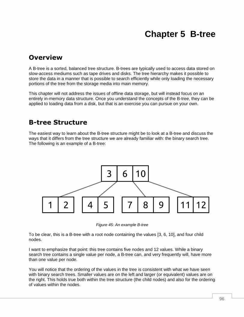
96

Chapter 5 B-tree

Overview

A B-tree is a sorted, balanced tree structure. B-trees are typically used to access data stored on slow-access mediums such as tape drives and disks. The tree hierarchy makes it possible to store the data in a manner that is possible to search efficiently while only loading the necessary portions of the tree from the storage media into main memory.

This chapter will not address the issues of offline data storage, but will instead focus on an entirely in-memory data structure. Once you understand the concepts of the B-tree, they can be applied to loading data from a disk, but that is an exercise you can pursue on your own.

B-tree Structure

The easiest way to learn about the B-tree structure might be to look at a B-tree and discuss the ways that it differs from the tree structure we are already familiar with: the binary search tree. The following is an example of a B-tree:

Figure 45: An example B-tree

To be clear, this is a B-tree with a root node containing the values [3, 6, 10], and four child nodes.

I want to emphasize that point: this tree contains five nodes and 12 values. While a binary search tree contains a single value per node, a B-tree can, and very frequently will, have more than one value per node.

You will notice that the ordering of the values in the tree is consistent with what we have seen with binary search trees. Smaller values are on the left and larger (or equivalent) values are on the right. This holds true both within the tree structure (the child nodes) and also for the ordering of values within the nodes.

97

In this example, the root node has three values and four children. This pattern of n values and n + 1 children is an immutable trait of a B-tree. Whether a node contains one or a thousand values, there will always be one more child than values. Take a moment to consider why this is true.

When navigating the tree, we start at the root node. The first value in the node is 3. Following the “smaller values on the left” rule, we need to have a node to the left to traverse down to (unless the node is a leaf node, in which case it has no children). Likewise, the value 3 needs to have a child to its right for the values greater than 3 (and less than its neighbor value, 6).

Notice that the right child of the value 3 is also the left child of the value 6. Similarly, the right child of the value 6 is the left child of the value 10. And finally the last value, 10, has a right child.

Minimal Degree

A critical and often confusing concept in a B-tree is the minimal degree. Also called the minimization factor, degree, order, and probably many other things, the key concept is the same.

The minimal degree is the minimum number of children that every node, except for the root node (which can have fewer, but not more), must have. Throughout this chapter I will refer to the minimal degree by the variable T.

More formally, each non-root node in the B-tree will contain at least T children and a maximum of 2 × T children. There are two important facts we can derive from this:

Every non-root node will have at least T - 1 values.

Every non-root node will have at most 2 × T - 1 values.

A node that has T - 1 values is at its minimal degree and cannot have a value removed from it. A node that has 2 × T - 1 is at its maximal degree and cannot have another value added to it. A node in this state is said to be “full.”

Tree Height

The B-tree structure enforces the rule that every leaf node in the tree will be at the same depth and each leaf node will contain data.

The tree we saw in Figure 45 had four leaf nodes all of which were at the same depth of 2. Two examples of invalid B-trees follow.

98

Figure 46: An invalid B-tree. The leaf nodes (green) are not all on the same level

Figure 47: An invalid B-tree. The leaf nodes (green) are at the same height but one is empty or missing

Searching the Tree

Because of its ordered structure, searching a B-tree is similar to searching a binary search tree. The algorithm for searching for a value in the tree is pretty simple. The algorithm recursively processes each node, starting at the root, using the following algorithm:

bool search(node, valueToFind)

foreach value in node

if valueToFind == value

return true

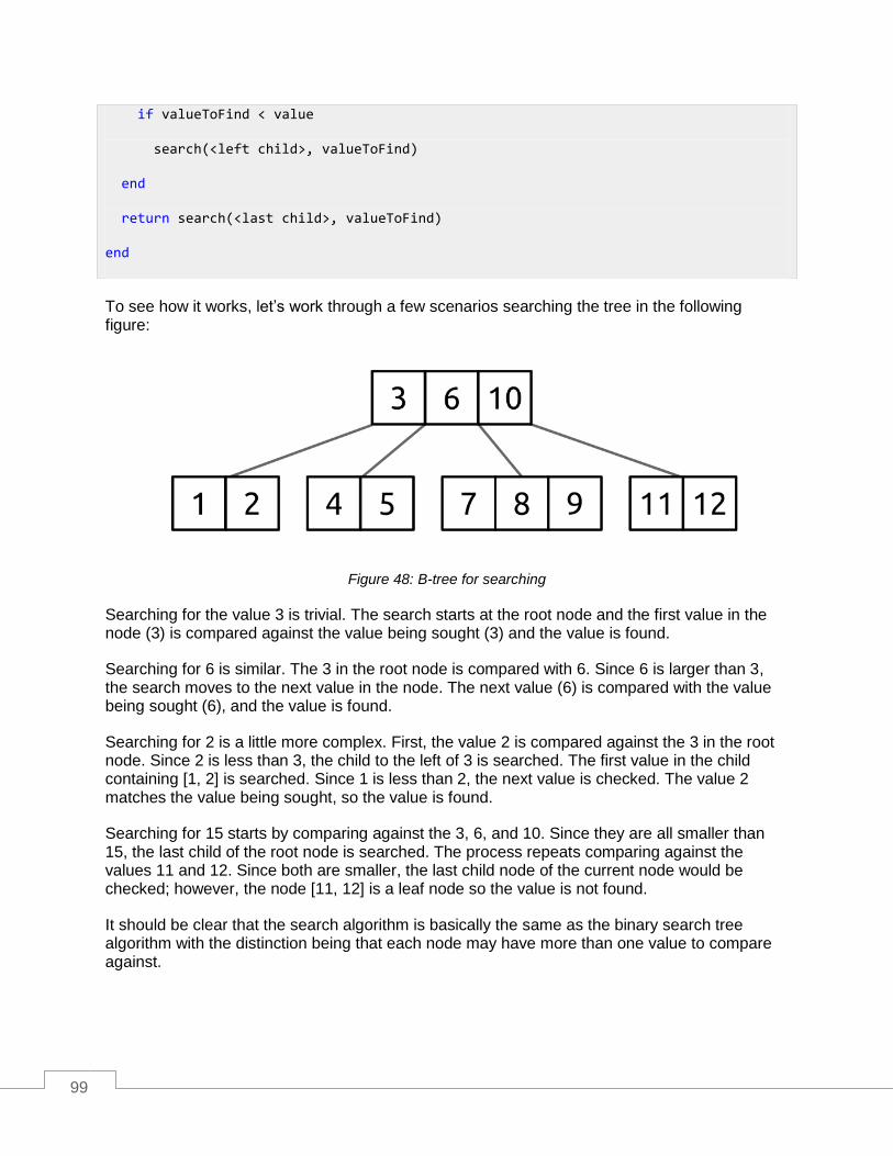
99

To see how it works, let’s work through a few scenarios searching the tree in the following figure:

Figure 48: B-tree for searching

Searching for the value 3 is trivial. The search starts at the root node and the first value in the node (3) is compared against the value being sought (3) and the value is found.

Searching for 6 is similar. The 3 in the root node is compared with 6. Since 6 is larger than 3, the search moves to the next value in the node. The next value (6) is compared with the value being sought (6), and the value is found.

Searching for 2 is a little more complex. First, the value 2 is compared against the 3 in the root node. Since 2 is less than 3, the child to the left of 3 is searched. The first value in the child containing [1, 2] is searched. Since 1 is less than 2, the next value is checked. The value 2 matches the value being sought, so the value is found.

Searching for 15 starts by comparing against the 3, 6, and 10. Since they are all smaller than 15, the last child of the root node is searched. The process repeats comparing against the values 11 and 12. Since both are smaller, the last child node of the current node would be checked; however, the node [11, 12] is a leaf node so the value is not found.

It should be clear that the search algorithm is basically the same as the binary search tree algorithm with the distinction being that each node may have more than one value to compare against.

if valueToFind < value

search(<left child>, valueToFind)

end

return search(<last child>, valueToFind)

end

100

Putting it Together

With the understanding of tree height, minimal degree, and how to search the tree, let’s take a few moments to consider how efficient this structure is.

Imagine a tree with a minimal factor of 501. This tree will have at least 500 values in each non-root node (with a maximum of 1000). If the root node contains 500 values, and each of its 501 children contained 500 values, the first two levels alone would contain 500 × 502, or 251,000, values.

To find a specific value we would start at the root node and perform at most 500 comparisons. Along the way we would either find the value we want or determine which node to check next. At that next node we would again perform at most 500 comparisons or determine the node was not there. This means we would perform at most 1000 comparisons in a tree with 251,000 values.

But it could be even better!

Since each node contains a sorted array of values, we could use a binary search instead of a linear search. We can now perform only 9 comparisons per node, and in only 18 comparisons—in the worst case—determine whether or not the value exists in a tree of 251,000 values.

Balancing Operations

Like an AVL tree, when an operation that changes the tree structure occurs, a B-tree may need to be balanced to ensure that it implements the structural rules. While conceptually similar, the actual operations are quite different from how an AVL works.

In this section, we are going to look at several types of balancing operations and discuss what purpose they serve.

Pushing Down

Pushing a value down is a process in which two child nodes are merged together with a value from the parent pushed down into the resulting node as the median value. Let’s take a look at what this means. We start with the following tree:

101

Figure 49: B-tree for pushing down

Say this is a tree with degree 3. This means that each node must have between 2 and 5 values (with the exception of the root node). With that understanding, how would we delete the value 2 from this tree? If we simply removed the 2 from the leaf node, the child node [1, 2] would be left with only a single value in it. Since that would violate the B-tree structural rules, it is not an acceptable solution.

What we need is for the value 2 to exist within a node that has at least T values in it that also abides by the other B-tree structural rules. To do this, we are going to create a new node by doing the following:

1. Allocate a new node.

2. Put the values [1, 2] into the new node.

3. Put the value [3] into the new node.

4. Put the values [4, 5] into the new node.

5. Discard the existing nodes [1, 2] and [4, 5].

6. Remove the value [3] from the parent node.

7. Link the new node where [4, 5] was previously linked.

This results in a tree that looks like the following:

Figure 50: Pushed down B-tree

102

We now have a node with 2 × T - 1 values in it, which is more than enough to delete the value 2.

Key points:

Push down merges two adjacent children.

Each of those children have T - 1 values.

The parent value is added as the median value.

The resulting node has 2 × T - 1 values.

Rotating Values

Value rotation is very similar to push down and is done for the same reasons, just in a slightly different situation.

Consider the following tree:

Figure 51: B-tree for rotating

Like we did with push down, let’s look at how we would remove the value 2 from the tree when the node that contains 2 has only T - 1 values.

The key to resolving this issue is that [1, 2]’s sibling node, [4, 5 ,6], has more than T - 1 values and therefore can have a value taken from it without violating the structural rules. This is done by rotating the value we want to take through the parent as shown below.

103

Figure 52: B-tree before rotation

The value we are going to rotate (4) is going to rotate to the parent node, and the parent value (3) is going to rotate to the child node, giving a resulting tree of:

Figure 53: B-tree after rotation

With this rotation done, the value 2 can now be deleted from the leaf node.

The specific steps that occurred here are:

1. Add the parent value to the end of the left child’s values.

a. This is adds the value 3 to the [1, 2] node, making the node [1, 2, 3].

2. Copy the first value of the right sibling’s values (4) to the parent (where 3 was).

a. At this point, 4 exists in both the root node [4] and still in [4, 5, 6].

3. If the [4,5,6] node is not a leaf node, move the left child of 4 to be the right child of 3 in

[1, 2, 3].

a. This works because everything that was left of 4 in [4, 5, 6] is, by definition, less

than 4 but greater than 3. Now that 4 is the root, we know that all the values on

that sub-tree belong to its left. Similarly, we know that all the values in that sub-

tree are greater than 3 so they belong to its right.

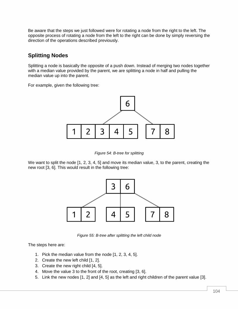
104

Be aware that the steps we just followed were for rotating a node from the right to the left. The opposite process of rotating a node from the left to the right can be done by simply reversing the direction of the operations described previously.

Splitting Nodes

Splitting a node is basically the opposite of a push down. Instead of merging two nodes together with a median value provided by the parent, we are splitting a node in half and pulling the median value up into the parent.

For example, given the following tree:

Figure 54: B-tree for splitting

We want to split the node [1, 2, 3, 4, 5] and move its median value, 3, to the parent, creating the new root [3, 6]. This would result in the following tree:

Figure 55: B-tree after splitting the left child node

The steps here are:

1. Pick the median value from the node [1, 2, 3, 4, 5].

2. Create the new left child [1, 2].

3. Create the new right child [4, 5].

4. Move the value 3 to the front of the root, creating [3, 6].

5. Link the new nodes [1, 2] and [4, 5] as the left and right children of the parent value [3].

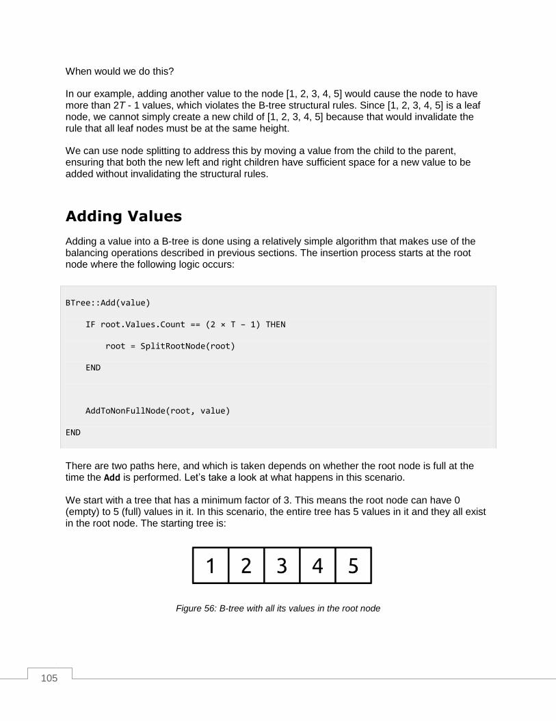
105

When would we do this?

In our example, adding another value to the node [1, 2, 3, 4, 5] would cause the node to have more than 2T - 1 values, which violates the B-tree structural rules. Since [1, 2, 3, 4, 5] is a leaf node, we cannot simply create a new child of [1, 2, 3, 4, 5] because that would invalidate the rule that all leaf nodes must be at the same height.

We can use node splitting to address this by moving a value from the child to the parent, ensuring that both the new left and right children have sufficient space for a new value to be added without invalidating the structural rules.

Adding Values

Adding a value into a B-tree is done using a relatively simple algorithm that makes use of the balancing operations described in previous sections. The insertion process starts at the root node where the following logic occurs:

There are two paths here, and which is taken depends on whether the root node is full at the time the Add is performed. Let’s take a look at what happens in this scenario.

We start with a tree that has a minimum factor of 3. This means the root node can have 0 (empty) to 5 (full) values in it. In this scenario, the entire tree has 5 values in it and they all exist in the root node. The starting tree is:

Figure 56: B-tree with all its values in the root node

BTree::Add(value)

IF root.Values.Count == (2 × T – 1) THEN

root = SplitRootNode(root)

END

AddToNonFullNode(root, value)

END

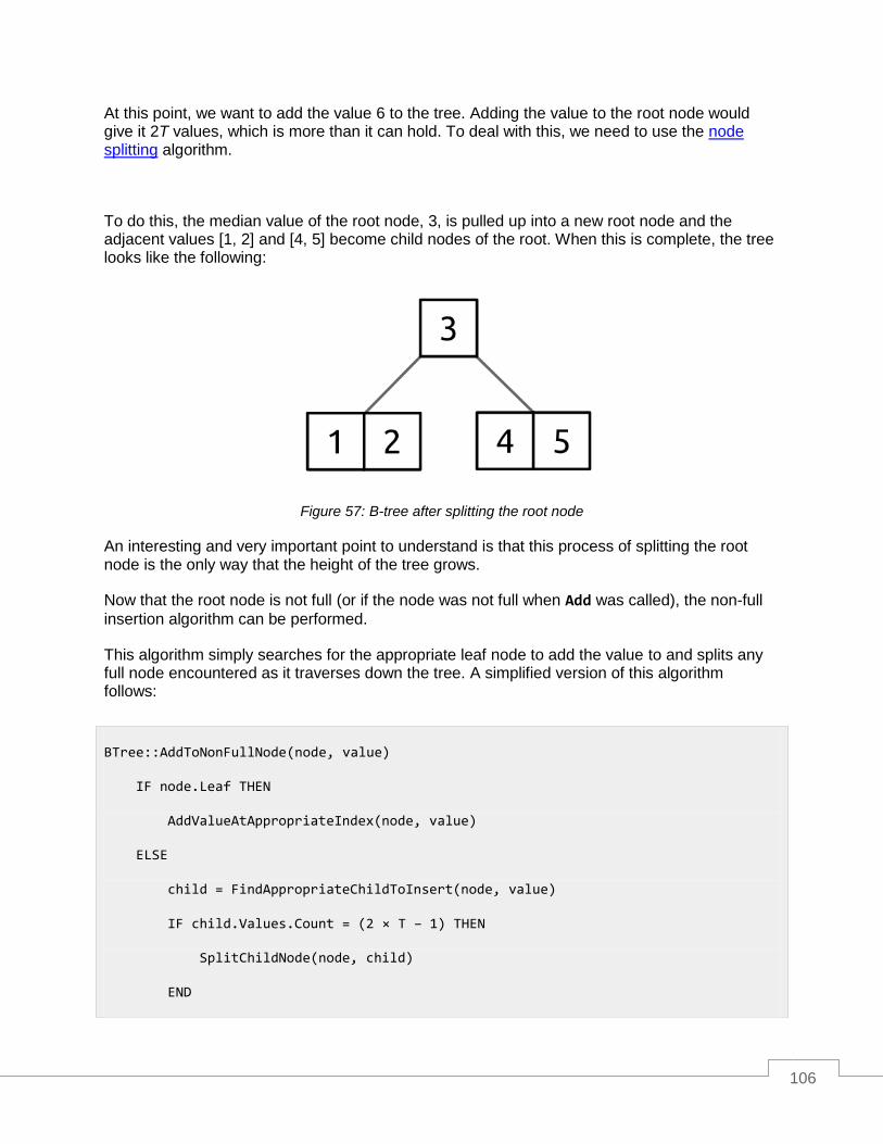
106

At this point, we want to add the value 6 to the tree. Adding the value to the root node would give it 2T values, which is more than it can hold. To deal with this, we need to use the node splitting algorithm.

To do this, the median value of the root node, 3, is pulled up into a new root node and the adjacent values [1, 2] and [4, 5] become child nodes of the root. When this is complete, the tree looks like the following:

Figure 57: B-tree after splitting the root node

An interesting and very important point to understand is that this process of splitting the root node is the only way that the height of the tree grows.

Now that the root node is not full (or if the node was not full when Add was called), the non-full

insertion algorithm can be performed.

This algorithm simply searches for the appropriate leaf node to add the value to and splits any full node encountered as it traverses down the tree. A simplified version of this algorithm follows:

BTree::AddToNonFullNode(node, value)

IF node.Leaf THEN

AddValueAtAppropriateIndex(node, value)

ELSE

child = FindAppropriateChildToInsert(node, value)

IF child.Values.Count = (2 × T – 1) THEN

SplitChildNode(node, child)

END

107

There are two key points you need to understand about this algorithm:

Values are only ever added to leaf nodes.

The algorithm never traverses into a full node; it always splits full nodes before going

into them. This is critical because it means the leaf node the value is inserted into cannot

be full.

Removing Values

Much like a binary search tree or AVL tree, removing a value from a B-tree is more complex than adding a value. In the case of a B-tree, there are three potential states that need to be dealt with:

1. The value to remove is in a leaf node.

a. In this case, we can simply remove the value.

2. The value is in an internal (non-leaf) node.

a. Push the value to be removed down one level (toward a leaf node). Use the

various balancing algorithms to ensure the tree stays structurally valid as the

value is pushed down.

b. Traverse into the child node where the value was pushed and repeat from step 1.

3. The value is not in the current internal node.

a. Find the child node where the value would be if it is in the tree.

b. Ensure the child node has at least T values in it.

i. Use the node rotation or merge algorithm on the child to ensure that it has

T nodes before traversing to it.

c. Traverse into the child node and repeat from step 1.

At a really high level, what is happening is we are walking down the tree, from the root to the appropriate leaf node, and along the way making sure of the following:

1. If we have found the value to remove, we push it down toward a leaf node.

2. If we have not, make sure the child node has T children before going to it.

The reason we do #1 is because we can only remove (and add) items in leaf nodes. This is not just because doing that is “easier,” but because doing it is mandatory. Each node has n values and n + 1 children. In a non-leaf node, each of those children references an entire subtree of nodes. If we removed a value from an internal node, we would have n - 1 values and n + 1 children. How would we manage that orphaned child tree?

AddToNonFullNode(child, value)

END

END

108

The only way we can safely remove (or add) an item from the tree is in a leaf node. This is because leaf nodes are the only ones that do not have this problem of managing children (because they have none).

And why do we do #2? We do it because if we don’t, then we can’t do #1. #1 says when we enter the internal node we will have n values, and when we are done we will have n - 1 values. If we started the process with T - 1 values (the minimum a node can contain), we would not be able to remove the node without violating the structural rules of the B-tree. So to make sure we can safely traverse to the child, we first ensure that the node has at least T values. This way if we push a value down, the node will still have at least T - 1 values and therefore still be valid.

B-tree Node

The B-tree has an internal node class that manages the values, pointers to the children, and a Boolean indicator for whether the node is a leaf node.

The BTreeNode class in the next example is pretty extensively commented and the concepts

used were detailed previously in this chapter. Because of that, large sections of code will stand on their own with little additional commentary.

BTreeNode Class

The BTreeNode class manages the operations to add and remove values from leaf nodes, push

down a value into a child node, and node splitting. Additionally, it provides some helper methods and properties used by the push down and splitting algorithms.

There is also a pair of validation methods used by the constructor and during operations that change the tree structure. They serve as a sanity check that the BTree class is not providing

inappropriate parameters to the constructor and that the tree has not moved from a valid to invalid state.

internal class BTreeNode<T> where T : IComparable<T> { private readonly List<T> _values; private readonly List<BTreeNode<T>> _children; internal BTreeNode(BTreeNode<T> parent, bool leaf, int minimumDegree, T[] values, BTreeNode<T>[] children) { ValidatePotentialState(parent, leaf, minimumDegree, values, children); Parent = parent; Leaf = leaf; MinimumDegree = minimumDegree; _values = new List<T>(values); _children = new List<BTreeNode<T>>(children); }

109

/// <summary> /// Returns true if the node has (2 * T - 1) nodes, false otherwise. /// </summary> internal bool Full { get; } /// <summary> /// True if the node is a leaf node, false otherwise. /// </summary> internal bool Leaf { get; private set; } /// <summary> /// The node's values. /// </summary> internal IList<T> Values { get; } /// <summary> /// The node's children. /// </summary> internal IList<BTreeNode<T>> Children { get; } /// <summary> /// The minimum degree of the node is the minimum degree of the tree. /// If the minimum degree is T then the node must have at least T - 1 /// values, but no more than 2 * T - 1. /// </summary> internal int MinimumDegree { get; private set; } /// <summary> /// The parent of the current node (or null if the root node). /// </summary> internal BTreeNode<T> Parent { get; set; } /// <summary> /// Splits a full child node, pulling the split value into the current node. /// </summary> /// <param name="indexOfChildToSplit">The child to split.</param> internal void SplitFullChild(int indexOfChildToSplit); /// <summary> /// Splits the full root node into a new root and two children. /// </summary> /// <returns>The new root node.</returns> internal BTreeNode<T> SplitFullRootNode(); /// <summary> /// Insert the specified value into the non-full leaf node. /// </summary> internal void InsertKeyToLeafNode(T value); /// <summary> /// Removes the specified value from the leaf node if it exists. /// </summary> /// <param name="value">The value to remove.</param> /// <returns>True if a value was removed, false otherwise.</returns> internal bool DeleteKeyFromLeafNode(T value); /// <summary>

110

Adding, Removing, and Updating Values

This section shows the code for methods that manage adding and removing values from leaf nodes. Additionally, a method for updating a value within the node (called by the BTree class

when moving values around) is shown.

/// Replaces the value at the specified index with the new value. /// </summary> internal void ReplaceValue(int valueIndex, T newValue); // [3 6] // [1 2] [4 5] [7 8] // becomes // [6] // [1 2 3 4 5] [7 8] internal BTreeNode<T> PushDown(int valueIndex); /// <summary> /// Adds the specified value to the front of the values and, if non-null, /// adds the specified value to the children. /// </summary> internal void AddFront(T newValue, BTreeNode<T> bTreeNode); /// <summary> /// Adds the specified value to the node and, if the specified node is non-null, /// adds the node to the children. /// </summary> internal void AddEnd(T valueToPushDown, BTreeNode<T> bTreeNode); /// <summary> /// Removes the first value and child (if applicable). /// </summary> internal void RemoveFirst(); /// <summary> /// Removes the last value and child (if applicable). /// </summary> internal void RemoveLast(); }

/// <summary> /// Insert the specified value into the non-full leaf node. /// </summary> /// <param name="value">The value to insert.</param> internal void InsertKeyToLeafNode(T value) { // Leaf validation is done by caller. if (!Leaf) { throw new InvalidOperationException("Unable to insert into a non-leaf node"); } // Non-full validation done by caller. if (Full) {

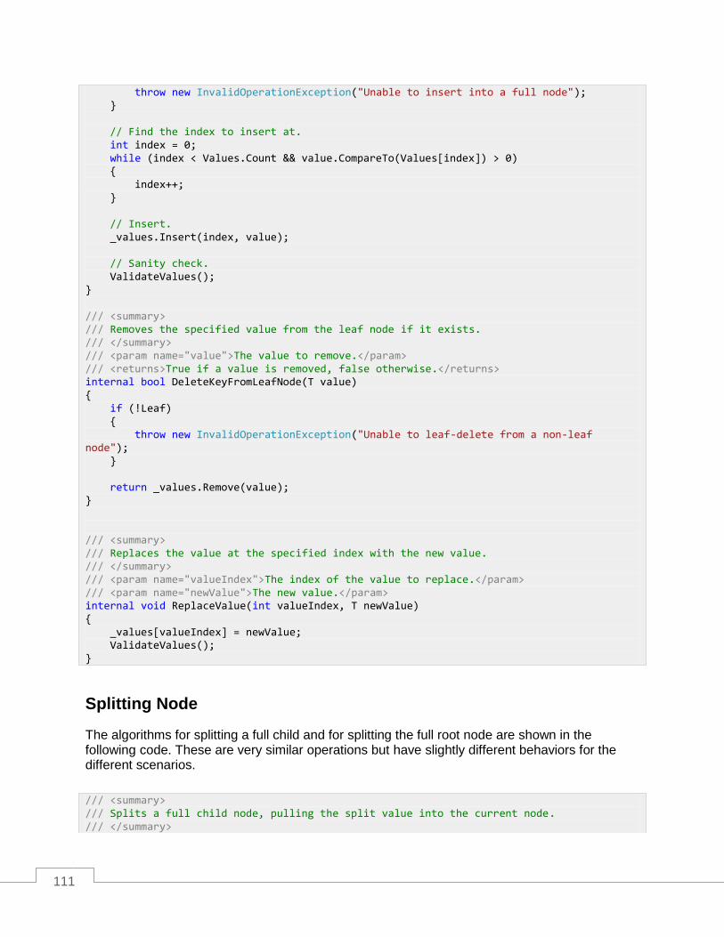
111

Splitting Node

The algorithms for splitting a full child and for splitting the full root node are shown in the following code. These are very similar operations but have slightly different behaviors for the different scenarios.

throw new InvalidOperationException("Unable to insert into a full node"); } // Find the index to insert at. int index = 0; while (index < Values.Count && value.CompareTo(Values[index]) > 0) { index++; } // Insert. _values.Insert(index, value); // Sanity check. ValidateValues(); } /// <summary> /// Removes the specified value from the leaf node if it exists. /// </summary> /// <param name="value">The value to remove.</param> /// <returns>True if a value is removed, false otherwise.</returns> internal bool DeleteKeyFromLeafNode(T value) { if (!Leaf) { throw new InvalidOperationException("Unable to leaf-delete from a non-leaf node"); } return _values.Remove(value); } /// <summary> /// Replaces the value at the specified index with the new value. /// </summary> /// <param name="valueIndex">The index of the value to replace.</param> /// <param name="newValue">The new value.</param> internal void ReplaceValue(int valueIndex, T newValue) { _values[valueIndex] = newValue; ValidateValues(); }

/// <summary> /// Splits a full child node, pulling the split value into the current node. /// </summary>

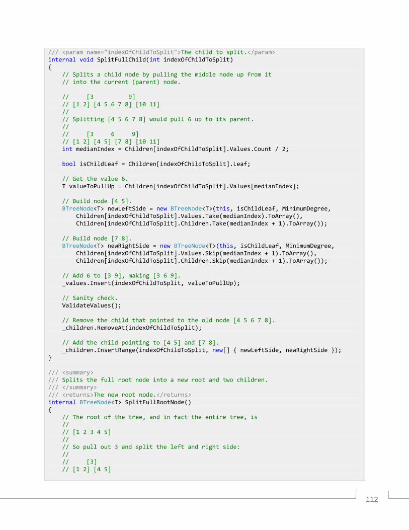
112

/// <param name="indexOfChildToSplit">The child to split.</param> internal void SplitFullChild(int indexOfChildToSplit) { // Splits a child node by pulling the middle node up from it // into the current (parent) node. // [3 9] // [1 2] [4 5 6 7 8] [10 11] // // Splitting [4 5 6 7 8] would pull 6 up to its parent. // // [3 6 9] // [1 2] [4 5] [7 8] [10 11] int medianIndex = Children[indexOfChildToSplit].Values.Count / 2; bool isChildLeaf = Children[indexOfChildToSplit].Leaf; // Get the value 6. T valueToPullUp = Children[indexOfChildToSplit].Values[medianIndex]; // Build node [4 5]. BTreeNode<T> newLeftSide = new BTreeNode<T>(this, isChildLeaf, MinimumDegree, Children[indexOfChildToSplit].Values.Take(medianIndex).ToArray(), Children[indexOfChildToSplit].Children.Take(medianIndex + 1).ToArray()); // Build node [7 8]. BTreeNode<T> newRightSide = new BTreeNode<T>(this, isChildLeaf, MinimumDegree, Children[indexOfChildToSplit].Values.Skip(medianIndex + 1).ToArray(), Children[indexOfChildToSplit].Children.Skip(medianIndex + 1).ToArray()); // Add 6 to [3 9], making [3 6 9]. _values.Insert(indexOfChildToSplit, valueToPullUp); // Sanity check. ValidateValues(); // Remove the child that pointed to the old node [4 5 6 7 8]. _children.RemoveAt(indexOfChildToSplit); // Add the child pointing to [4 5] and [7 8]. _children.InsertRange(indexOfChildToSplit, new[] { newLeftSide, newRightSide }); } /// <summary> /// Splits the full root node into a new root and two children. /// </summary> /// <returns>The new root node.</returns> internal BTreeNode<T> SplitFullRootNode() { // The root of the tree, and in fact the entire tree, is // // [1 2 3 4 5] // // So pull out 3 and split the left and right side: // // [3] // [1 2] [4 5]

113

Pushing Down

This code implements the push down algorithm documented previously.

// Find the index of the value to pull up: 3. int medianIndex = Values.Count / 2; // Now get the 3. T rootValue = Values[medianIndex]; // Build the new root node (empty). BTreeNode<T> result = new BTreeNode<T>(Parent, false, MinimumDegree, new T[0], new BTreeNode<T>[0]); // Build the left node [1 2]. BTreeNode<T> newLeftSide = new BTreeNode<T>(result, Leaf, MinimumDegree, Values.Take(medianIndex).ToArray(), Children.Take(medianIndex + 1).ToArray()); // Build the right node [4 5]. BTreeNode<T> newRightSide = new BTreeNode<T>(result, Leaf, MinimumDegree, Values.Skip(medianIndex + 1).ToArray(), Children.Skip(medianIndex + 1).ToArray()); // Add the 3 to the root node. result._values.Add(rootValue); // Add the left child [1 2]. result._children.Add(newLeftSide); // Add the right child [4 5]. result._children.Add(newRightSide); return result; }

// [3 6] // [1 2] [4 5] [7 8] // becomes // [6] // [1 2 3 4 5] [7 8] internal BTreeNode<T> PushDown(int valueIndex) { List<T> values = new List<T>(); // [1 2] -> [1 2] values.AddRange(Children[valueIndex].Values); // [3] -> [1 2 3] values.Add(Values[valueIndex]); // [4 5] -> [1 2 3 4 5] values.AddRange(Children[valueIndex + 1].Values); List<BTreeNode<T>> children = new List<BTreeNode<T>>(); children.AddRange(Children[valueIndex].Children);

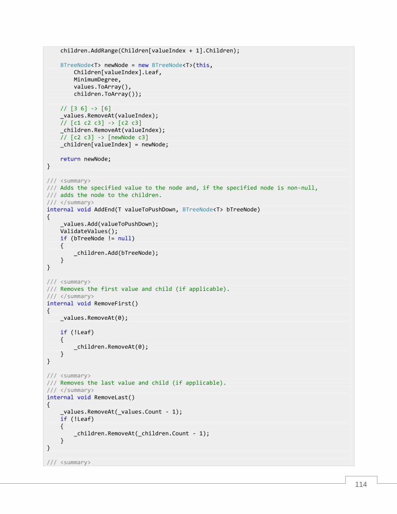
114

children.AddRange(Children[valueIndex + 1].Children); BTreeNode<T> newNode = new BTreeNode<T>(this, Children[valueIndex].Leaf, MinimumDegree, values.ToArray(), children.ToArray()); // [3 6] -> [6] _values.RemoveAt(valueIndex); // [c1 c2 c3] -> [c2 c3] _children.RemoveAt(valueIndex); // [c2 c3] -> [newNode c3] _children[valueIndex] = newNode; return newNode; } /// <summary> /// Adds the specified value to the node and, if the specified node is non-null, /// adds the node to the children. /// </summary> internal void AddEnd(T valueToPushDown, BTreeNode<T> bTreeNode) { _values.Add(valueToPushDown); ValidateValues(); if (bTreeNode != null) { _children.Add(bTreeNode); } } /// <summary> /// Removes the first value and child (if applicable). /// </summary> internal void RemoveFirst() { _values.RemoveAt(0); if (!Leaf) { _children.RemoveAt(0); } } /// <summary> /// Removes the last value and child (if applicable). /// </summary> internal void RemoveLast() { _values.RemoveAt(_values.Count - 1); if (!Leaf) { _children.RemoveAt(_children.Count - 1); } } /// <summary>

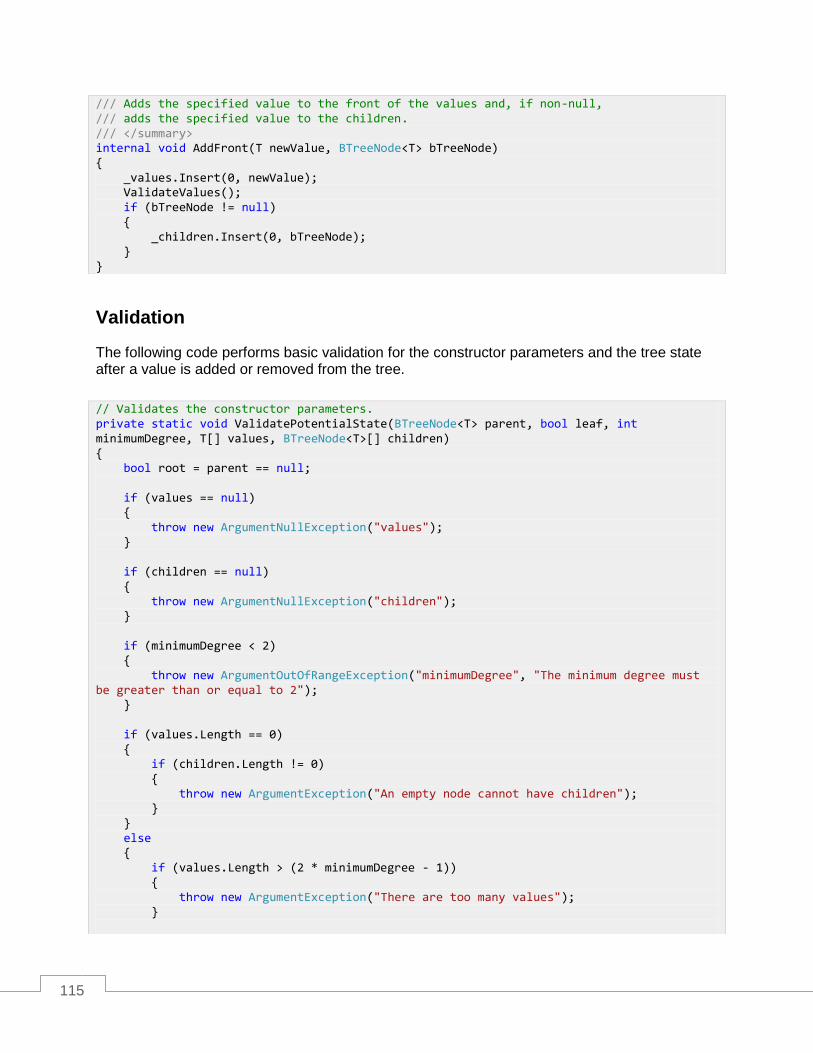
115

Validation

The following code performs basic validation for the constructor parameters and the tree state after a value is added or removed from the tree.

/// Adds the specified value to the front of the values and, if non-null, /// adds the specified value to the children. /// </summary> internal void AddFront(T newValue, BTreeNode<T> bTreeNode) { _values.Insert(0, newValue); ValidateValues(); if (bTreeNode != null) { _children.Insert(0, bTreeNode); } }

// Validates the constructor parameters. private static void ValidatePotentialState(BTreeNode<T> parent, bool leaf, int minimumDegree, T[] values, BTreeNode<T>[] children) { bool root = parent == null; if (values == null) { throw new ArgumentNullException("values"); } if (children == null) { throw new ArgumentNullException("children"); } if (minimumDegree < 2) { throw new ArgumentOutOfRangeException("minimumDegree", "The minimum degree must be greater than or equal to 2"); } if (values.Length == 0) { if (children.Length != 0) { throw new ArgumentException("An empty node cannot have children"); } } else { if (values.Length > (2 * minimumDegree - 1)) { throw new ArgumentException("There are too many values"); }

116

B-tree

The BTree class is what pulls together everything we’ve looked at in this chapter. As with

BTreeNode, because the code is extensively commented and the core concepts are covered

previously in this chapter, the code will basically stand on its own.

BTree Class

The BTree class implements the ICollection<T> interface and therefore provides the basic

operations to add, remove, search, copy, count, clear, and enumerate (using an inorder traversal). Additionally, it has a reference to the root node (which will be null when the tree is empty), and a constant value that dictates the minimum degree of the tree (which in turn defines the minimum degree for every node).

if (!root) { if (values.Length < minimumDegree - 1) { throw new ArgumentException("Each non-root node must have at least degree - 1 children"); } } if (!leaf && !root) { if (values.Length + 1 != children.Length) { throw new ArgumentException("There should be one more child than values"); } } } } [Conditional("DEBUG")] private void ValidateValues() { if (_values.Count > 1) { for (int i = 1; i < _values.Count; i++) { Debug.Assert(_values[i - 1].CompareTo(_values[i]) < 0); } } }

public class BTree<T> : ICollection<T> where T : IComparable<T> { BTreeNode<T> root = null; const int MinimumDegree = 2;

117

Add

Behavior Adds the specified value to the tree.


This code implements the insertion algorithm previously described.

public void Add(T value); public bool Remove(T value); public bool Contains(T value); public void Clear(); public void CopyTo(T[] array, int arrayIndex); public int Count { get; private set; } public bool IsReadOnly { get; } public IEnumerator<T> GetEnumerator(); System.Collections.IEnumerator System.Collections.IEnumerable.GetEnumerator(); }

public void Add(T value) { if (root == null) { root = new BTreeNode<T>(null, true, MinimumDegree, new[] { value }, new BTreeNode<T>[] { }); } else { if (root.Full) { root = root.SplitFullRootNode(); } InsertNonFull(root, value); } Count++; } private void InsertNonFull(BTreeNode<T> node, T value) { if (node.Leaf)

118

Remove

Behavior Removes the first occurrence of the specified value from the tree. Returns true if a value was found and removed. Otherwise it returns false.


This code implements the remove algorithm previously described.

{ node.InsertKeyToLeafNode(value); } else { int index = node.Values.Count - 1; while (index >= 0 && value.CompareTo(node.Values[index]) < 0) { index--; } index++; if (node.Children[index].Full) { node.SplitFullChild(index); if (value.CompareTo(node.Values[index]) > 0) { index++; } } InsertNonFull(node.Children[index], value); } }

public bool Remove(T value) { bool removed = false; if (Count > 0) { removed = RemoveValue(root, value); if (removed) { Count--; if (Count == 0) { root = null; } else if (root.Values.Count == 0)

119

{ root = root.Children[0]; } } } return removed; } internal static bool RemoveValue(BTreeNode<T> node, T value) { if (node.Leaf) { // Deletion case 1... // By the time we are in a leaf node, we have either pushed down // values such that the leaf node has minimum degree children // and can therefore have one node removed, OR the root node is // also a leaf node and we can freely violate the minimum rule. return node.DeleteKeyFromLeafNode(value); } int valueIndex; if (TryGetIndexOf(node, value, out valueIndex)) { // Deletion case 2... // We have found the non-leaf node the value is in. Since we can only delete values // from a leaf node, we need to push the value to delete down into a child. // If the child that precedes the value to delete (the "left" child) has // at least the minimum degree of children... if (node.Children[valueIndex].Values.Count >= node.Children[valueIndex].MinimumDegree) { // [3 6 10] // [1 2] [4 5] [7 8 9] [11 12] // Deleting 10. // Find the largest value in the child node that contains smaller values // than what is being deleted (this is the value 9)... T valuePrime = FindPredecessor(node, valueIndex); // and REPLACE the value to delete with the next largest value (the one // we just found--swapping 9 and 10). node.ReplaceValue(valueIndex, valuePrime); // After the swap... // [3 6 9] // [1 2] [4 5] [7 8 9] [11 12] // notice that 9 is in the tree twice. This is not a typo. We are about // to delete it from the child we took it from.

120

// Delete the value we moved up (9) from the child (this may in turn // push it down to subsequent children until it is in a leaf). return RemoveValue(node.Children[valueIndex], valuePrime); // Final tree: // [3 6 9] // [1 2] [4 5] [7 8 ] [11 12] } else { // If the left child did not have enough values to move one of its values up, // check whether the right child does. if (node.Children[valueIndex + 1].Values.Count >= node.Children[valueIndex + 1].MinimumDegree) { // See the previous algorithm and do the opposite... // [3 6 10] // [1 2] [4 5] [7 8 9] [11 12] // Deleting 6. // Successor = 7. T valuePrime = FindSuccessor(node, valueIndex); node.ReplaceValue(valueIndex, valuePrime); // After replacing 6 with 7, the tree is: // [3 7 10] // [1 2] [4 5] [7 8 9] [11 12] // Now remove 7 from the child. return RemoveValue(node.Children[valueIndex + 1], valuePrime); // Final tree: // [3 7 10] // [1 2] [4 5] [8 9] [11 12] } else { // If neither child has the minimum degree of children, it means they // both have (minimum degree - 1) children. Since a node can have // (2 * <minimum degree> - 1) children, we can safely merge the two nodes // into a single child. // // [3 6 9] // [1 2] [4 5] [7 8] [10 11] // // Deleting 6. // // [4 5] and [7 8] are merged into a single node with [6] pushed down //into it. // // [3 9]

121

// [1 2] [4 5 6 7 8] [10 11] // BTreeNode<T> newChildNode = node.PushDown(valueIndex); // Now that we've pushed the value down a level, we can call remove // on the new child node [4 5 6 7 8]. return RemoveValue(newChildNode, value); } } } else { // Deletion case 3... // We are at an internal node which does not contain the value we want to delete. // First, find the child path that the value we want to delete would be in. // If it exists in the tree... int childIndex; FindPotentialPath(node, value, out valueIndex, out childIndex); // Now that we know where the value should be, we need to ensure that the node // we are going to has the minimum number of values necessary to delete from. if (node.Children[childIndex].Values.Count == node.Children[childIndex].MinimumDegree - 1) { // Since the node does not have enough values, what we want to do is borrow // a value from a sibling that has enough values to share. // Determine if the left or right sibling has the most children. int indexOfMaxSibling = GetIndexOfMaxSibling(childIndex, node); // If a sibling with values exists (maybe we're // at the root node and don't have one) // and that sibling has enough values... if (indexOfMaxSibling >= 0 && node.Children[indexOfMaxSibling].Values.Count >= node.Children[indexOfMaxSibling].MinimumDegree) { // Rotate the appropriate value from the sibling // through the parent and into the current node // so that we have enough values in the current // node to push a value down into the // child we are going to check next. // [3 7] // [1 2] [4 5 6] [8 9] // // The node we want to travel through is [1 2], but we // need another node in it. So we rotate the 4 // up to the root and push the 3 down into the [1 2] // node. // // [4 7] // [1 2 3] [5 6] [7 8] RotateAndPushDown(node, childIndex, indexOfMaxSibling); } else

122

{ // Merge (which may push the only node in the root down--so new root). BTreeNode<T> pushedDownNode = node.PushDown(valueIndex); // Now find the node we just pushed down. childIndex = 0; while (pushedDownNode != node.Children[childIndex]) { childIndex++; } } } return RemoveValue(node.Children[childIndex], value); } } internal static void RotateAndPushDown(BTreeNode<T> node, int childIndex, int indexOfMaxSibling) { int valueIndex; if (childIndex < indexOfMaxSibling) { valueIndex = childIndex; } else { valueIndex = childIndex - 1; } if (indexOfMaxSibling > childIndex) { // We are moving the leftmost key from the right sibling into the parent // and pushing the parent down into the child. // // [6 10] // [1] [7 8 9] [11] // // Deleting something less than 6. // // [7 10] // [1 6] [8 9] [11] // Grab the 7. T valueToMoveToX = node.Children[indexOfMaxSibling].Values.First(); // Get 7's left child if it has one (not a leaf). BTreeNode<T> childToMoveToNode = node.Children[indexOfMaxSibling].Leaf ? null : node.Children[indexOfMaxSibling].Children.First(); // Record the 6 (the push down value). T valueToMoveDown = node.Values[valueIndex]; // Move the 7 into the parent. node.ReplaceValue(valueIndex, valueToMoveToX); // Move the 6 into the child. node.Children[childIndex].AddEnd(valueToMoveDown, childToMoveToNode);

123

// Remove the first value and child from the sibling now that they've been moved. node.Children[indexOfMaxSibling].RemoveFirst(); } else { // We are moving the rightmost key from the left sibling into the parent // and pushing the parent down into the child. // // [6 10] // [1] [7 8 9] [11] // // Deleting something greater than 10. // // [6 9] // [1] [7 8] [10, 11] // Grab the 9. T valueToMoveToX = node.Children[indexOfMaxSibling].Values.Last(); // Get 9's right child if it has one (not a leaf node). BTreeNode<T> childToMoveToNode = node.Children[indexOfMaxSibling].Leaf ? null : node.Children[indexOfMaxSibling].Children.Last(); // Record the 10 (the push down value). T valueToMoveDown = node.Values[valueIndex]; // Move the 9 into the parent. node.ReplaceValue(valueIndex, valueToMoveToX); // Move the 10 into the child. node.Children[childIndex].AddFront(valueToMoveDown, childToMoveToNode); // Remove the last value and child from the sibling now that they've been moved. node.Children[indexOfMaxSibling].RemoveLast(); } } internal static void FindPotentialPath(BTreeNode<T> node, T value, out int valueIndex, out int childIndex) { // We want to find out which child the value we are searching for (value) // would be in if the value were in the tree. childIndex = node.Children.Count - 1; valueIndex = node.Values.Count - 1; // Start at the rightmost child and value indexes and work // backward until we are at less than the value we want. while (valueIndex > 0) { int compare = value.CompareTo(node.Values[valueIndex]); if (compare > 0) { break; }

124

childIndex--; valueIndex--; } // If we make it all the way to the last value... if (valueIndex == 0) { // If the value we are searching for is less than the first // value in the node, then the child is the 0 index child, // not the 1 index. if (value.CompareTo(node.Values[valueIndex]) < 0) { childIndex--; } } } // Returns the index (to the left or right) of the child node // that has the most values in it. // // Example // // [3 7] // [1 2] [4 5 6] [8 9] // // If we pass in the [3 7] node with index 0, the left child [1 2] // and right child [4 5 6] would be checked and the index 1 for child // node [4 5 6] would be returned. // // If we checked [3 7] with index 1, the left child [4 5 6] and the // right child [8 9] would be checked and the value 1 would be returned. private static int GetIndexOfMaxSibling(int index, BTreeNode<T> node) { int indexOfMaxSibling = -1; BTreeNode<T> leftSibling = null; if (index > 0) { leftSibling = node.Children[index - 1]; } BTreeNode<T> rightSibling = null; if (index + 1 < node.Children.Count) { rightSibling = node.Children[index + 1]; } if (leftSibling != null || rightSibling != null) { if (leftSibling != null && rightSibling != null) { indexOfMaxSibling = leftSibling.Values.Count > rightSibling.Values.Count ? index - 1 : index + 1; } else { indexOfMaxSibling = leftSibling != null ? index - 1 : index + 1; }

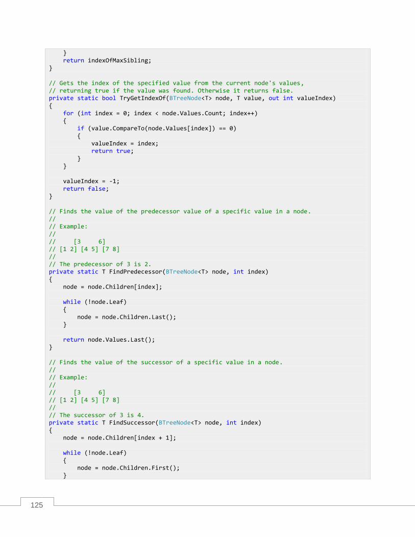
125

} return indexOfMaxSibling; } // Gets the index of the specified value from the current node's values, // returning true if the value was found. Otherwise it returns false. private static bool TryGetIndexOf(BTreeNode<T> node, T value, out int valueIndex) { for (int index = 0; index < node.Values.Count; index++) { if (value.CompareTo(node.Values[index]) == 0) { valueIndex = index; return true; } } valueIndex = -1; return false; } // Finds the value of the predecessor value of a specific value in a node. // // Example: // // [3 6] // [1 2] [4 5] [7 8] // // The predecessor of 3 is 2. private static T FindPredecessor(BTreeNode<T> node, int index) { node = node.Children[index]; while (!node.Leaf) { node = node.Children.Last(); } return node.Values.Last(); } // Finds the value of the successor of a specific value in a node. // // Example: // // [3 6] // [1 2] [4 5] [7 8] // // The successor of 3 is 4. private static T FindSuccessor(BTreeNode<T> node, int index) { node = node.Children[index + 1]; while (!node.Leaf) { node = node.Children.First(); }

126

Contains

Behavior Returns true if the specified value exists in the tree. Otherwise it returns

false.


return node.Values.First(); }

public bool Contains(T value) { BTreeNode<T> node; int valueIndex; return TryFindNodeContainingValue(value, out node, out valueIndex); } // Searches the node and its children, looking for the specified value. internal bool TryFindNodeContainingValue(T value, out BTreeNode<T> node, out int valueIndex) { BTreeNode<T> current = root; // If the current node is null, then we never found the value. // Otherwise, we still have hope. while (current != null) { int index = 0; // Check each value in the node. while (index < current.Values.Count) { int compare = value.CompareTo(current.Values[index]); // Did we find it? if (compare == 0) { // Awesome! node = current; valueIndex = index; return true; } // If the value to find is less than the current node's value, // then we want to go left (which is where we are). if (compare < 0) { break;

127

Clear

Behavior Removes all values from the tree and sets the count to 0.

Performance O(1)

Count

Behavior Returns the number of values in the tree (0 if the tree is empty).

Performance O(1)

} // Otherwise, move on to the next value in the node. index++; } if (current.Leaf) { // If we are at a leaf node, there is no child to go // down to. break; } else { // Otherwise, go into the child we determined must contain the // value we want to find. current = current.Children[index]; } } node = null; valueIndex = -1; return false; }

public void Clear() { root = null; Count = 0; }

128

CopyTo

Behavior Copies every value in the tree into the target array, starting at the specified index.

Performance O(n)

IsReadOnly

Behavior Returns a value indicating whether the tree is read-only.

Performance O(1)

public int Count { get; private set; }

public void CopyTo(T[] array, int arrayIndex) { foreach (T value in InOrderEnumerator(root)) { array[arrayIndex++] = value; } }

public bool IsReadOnly { get { return false; } }

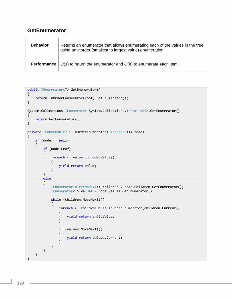
129

GetEnumerator

Behavior Returns an enumerator that allows enumerating each of the values in the tree using an inorder (smallest to largest value) enumeration.

Performance O(1) to return the enumerator and O(n) to enumerate each item.

public IEnumerator<T> GetEnumerator() { return InOrderEnumerator(root).GetEnumerator(); } System.Collections.IEnumerator System.Collections.IEnumerable.GetEnumerator() { return GetEnumerator(); } private IEnumerable<T> InOrderEnumerator(BTreeNode<T> node) { if (node != null) { if (node.Leaf) { foreach (T value in node.Values) { yield return value; } } else { IEnumerator<BTreeNode<T>> children = node.Children.GetEnumerator(); IEnumerator<T> values = node.Values.GetEnumerator(); while (children.MoveNext()) { foreach (T childValue in InOrderEnumerator(children.Current)) { yield return childValue; } if (values.MoveNext()) { yield return values.Current; } } } } }

data structures succinctly part 2

Documents

internal void splitfullchild

public void copyto

public hashtable

splits

removes

returns

adds

internal bool deletekeyfromleafnode