D A T A S T R U C T U R E S

D A T A S T R U C T U R E S

Decleration of the Arrays: Any array declaration contains: the array name, the element type and the array size.

Examples: int a[20], b[3],c[7];

float f[5], c[2]; char

m[4], n[20]; Initialization of an array is the process of assigning initial values. Typically declaration and initialization are combined. Examples: float, b[3]={2.0, 5.5, 3.14};

char name[4]= {„E‟,‟m‟,‟r‟,‟e‟}; int c[10]={0};

Dynamic Arrays Dynamic array allocation is actually a combination of pointers and dynamic memory allocation. Whereas static arrays are declared prior to runtime and are reserved in stack memory, dynamic arrays are created in the heap using the new and released from the heap using delete operators.

Start by declaring a pointer to whatever data type you want the array to hold. In this case I've used int :

int *my_array;

This C++ statement simply declares an integer pointer. Remember, a pointer is a variable that

holds a memory address. Declaring a pointer doesn't reserve any memory for the array - that will be accomplished with new. The following C++ statement requests 10 integer-sized elements be reserved in the heap with the first element address being assigned to the pointer my_array:

my_array = new int[10];

The new operator is requesting 10 integer elements from the heap. There is a possibility that there might not be enough memory left in the heap, in which case your program would have to properly handle such an error. Assuming everything went OK, you could then use the dynamically declared array just like the static array.

Dynamic array allocation is nice because the size of the array can be determined at runtime and

then used with the new operator to reserve the space in the heap. To illustrate I'll uses dynamic array allocation to set the size of its array at runtime.

// array allocation to set the size of its array at runtime.

#include <iostream.h> int main () {

int i,n;

int * p; cout << "How many numbers would you like to type?“;

cin >> i;

p= new int[i]; // it takes memory at run-time from Heap

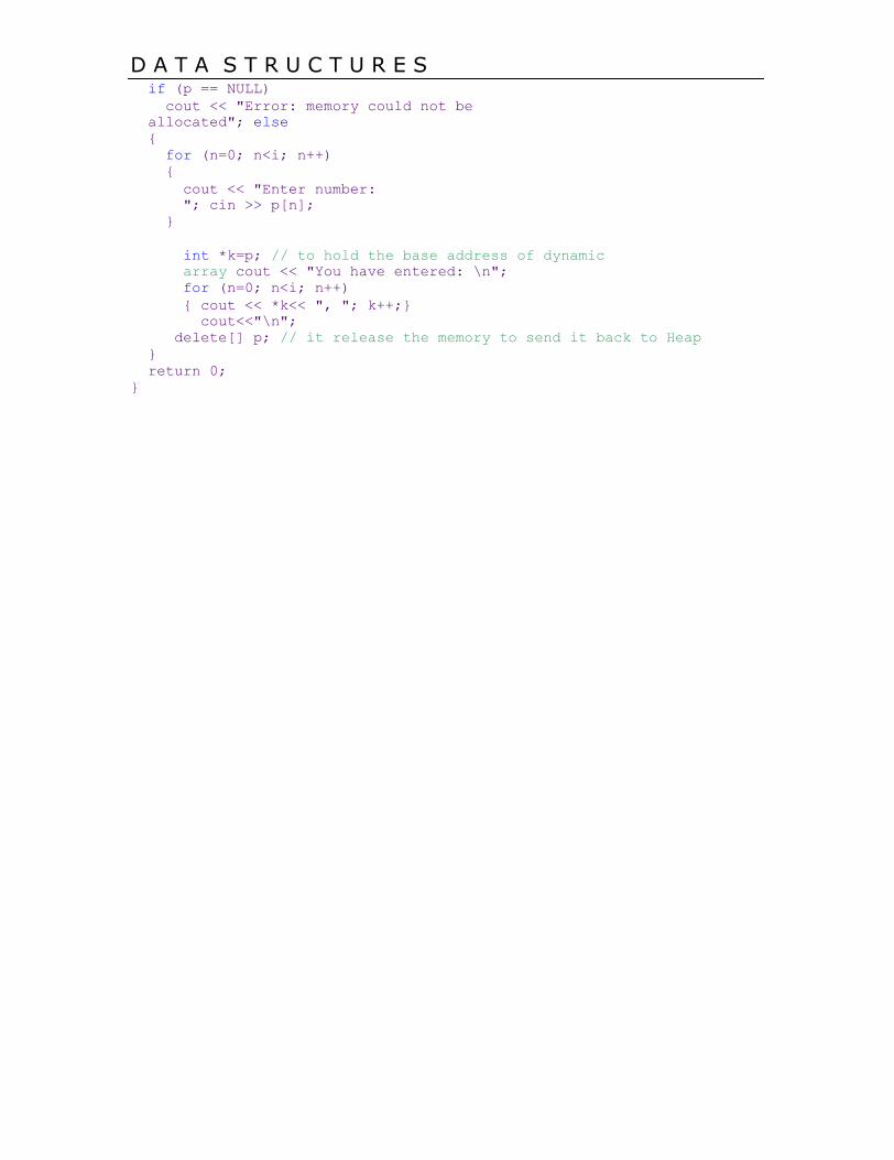
D A T A S T R U C T U R E S if (p == NULL)

cout << "Error: memory could not be

allocated"; else {

for (n=0; n<i; n++) {

cout << "Enter number:

"; cin >> p[n]; }

int *k=p; // to hold the base address of dynamic

array cout << "You have entered: \n"; for (n=0; n<i; n++) { cout << *k<< ", "; k++;}

cout<<"\n"; delete[] p; // it release the memory to send it back to Heap

} return 0;

}

D A T A S T R U C T U R E S

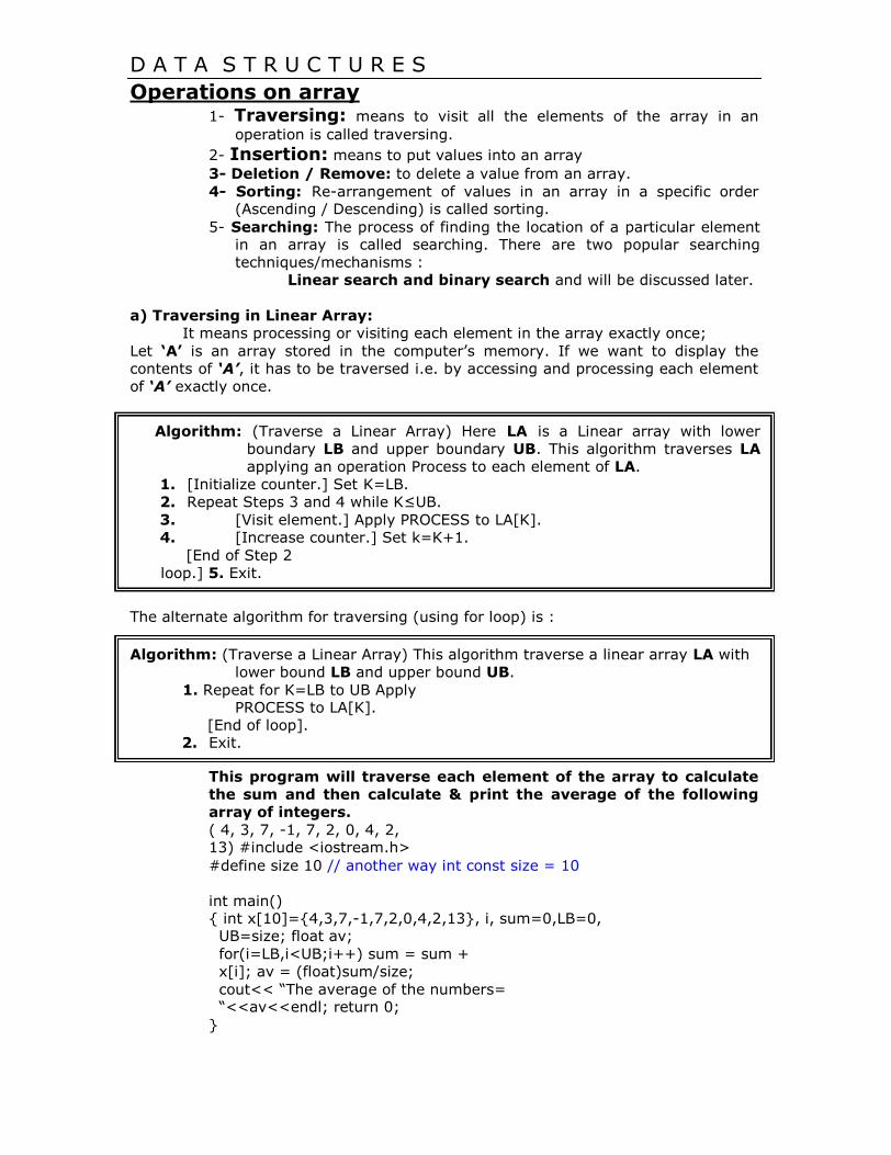
Operations on array 1- Traversing: means to visit all the elements of the array in an

operation is called traversing.

2- Insertion: means to put values into an array 3- Deletion / Remove: to delete a value from an array. 4- Sorting: Re-arrangement of values in an array in a specific order

(Ascending / Descending) is called sorting. 5- Searching: The process of finding the location of a particular element

in an array is called searching. There are two popular searching

techniques/mechanisms : Linear search and binary search and will be discussed later.

a) Traversing in Linear Array:

It means processing or visiting each element in the array exactly once; Let ‘A’ is an array stored in the computer‟s memory. If we want to display the

contents of ‘A’, it has to be traversed i.e. by accessing and processing each element

of ‘A’ exactly once.

Algorithm: (Traverse a Linear Array) Here LA is a Linear array with lower

boundary LB and upper boundary UB. This algorithm traverses LA

applying an operation Process to each element of LA. 1. [Initialize counter.] Set K=LB.

2. Repeat Steps 3 and 4 while K≤UB. 3. [Visit element.] Apply PROCESS to LA[K]. 4. [Increase counter.] Set k=K+1.

[End of Step 2

loop.] 5. Exit.

The alternate algorithm for traversing (using for loop) is : Algorithm: (Traverse a Linear Array) This algorithm traverse a linear array LA with

lower bound LB and upper bound UB. 1. Repeat for K=LB to UB Apply

PROCESS to LA[K]. [End of loop].

2. Exit.

This program will traverse each element of the array to calculate

the sum and then calculate & print the average of the following

array of integers. ( 4, 3, 7, -1, 7, 2, 0, 4, 2, 13) #include <iostream.h> #define size 10 // another way int const size = 10

int main() { int x[10]={4,3,7,-1,7,2,0,4,2,13}, i, sum=0,LB=0, UB=size; float av; for(i=LB,i<UB;i++) sum = sum +

x[i]; av = (float)sum/size; cout<< “The average of the numbers= “<<av<<endl; return 0;

}

D A T A S T R U C T U R E S b) Sorting in Linear Array:

Sorting an array is the ordering the array elements in ascending (increasing - from min to max) or descending (decreasing – from max to min) order. Example: {2 1 5 7 4 3} {1, 2, 3, 4, 5,7} ascending order

{2 1 5 7 4 3} {7,5, 4, 3, 2, 1} descending order Bubble Sort:

The technique we use is called “Bubble Sort” because the bigger value

gradually bubbles their way up to the top of array like air bubble rising in water,

while the small values sink to the bottom of array. This technique is to make several passes through the array. On each pass,

successive pairs of elements are compared. If a pair is in increasing order (or the

values are identical), we leave the values as they are. If a pair is in decreasing

order, their values are swapped in the array.

B u b b le S o r t

P a s s = 1 P a s s = 2 P a s s = 3 P a s s = 4

2 1 5 7 4 3 1 2 5 4 3 7 1 2 4 3 5 7 1 2 3 4 5 7

1 2 5 7 4 3 1 2 5 4 3 7 1 2 4 3 5 7 1 2 3 4 5 7

1 2 5 7 4 3 1 2 5 4 3 7 1 2 4 3 5 7 1 2 3 4 5 7

1 2 5 7 4 3 1 2 4 5 3 7 1 2 3 4 5 7

1 2 5 4 7 3 1 2 4 3 5 7

1 2 5 4 3 7

U n d e rlin e d p a irs s h o w th e c o m p a ris o n s . F o r e a c h p a s s th e re a res

ize - 1c o m p a ris o n s . To ta l n u m b e r o f c o m p a ris o n s =(s ize - 1 )

2

Algorithm: (Bubble Sort) BUBBLE (DATA, N)

Here DATA is an Array with N elements. This algorithm sorts

the elements in DATA. 1. for pass=1 to N-1. 2. for (i=0; i<= N-Pass; i++) 3. If DATA[i]>DATA[i+1], then:

Interchange DATA[i] and DATA[i+1]. [End of If Structure.]

[End of inner loop.]

[End of Step 1 outer loop.] 4. Exit.

D A T A S T R U C T U R E S /* This program sorts the array elements in the ascending order using

bubble sort method */

#include <iostream.h>

int const SIZE = 6 void BubbleSort(int [ ], int); int main() { int a[SIZE]= {77,42,35,12,101,6}; int i; cout<< “The elements of the array before sorting\n”;

for (i=0; i<= SIZE-1; i++)

cout<< a[i]<<”, “;

BubbleSort(a, SIZE); cout<< “\n\nThe elements of the array after sorting\n”; for (i=0; i<= SIZE-1; i++)

cout<< a[i]<<”, “; return 0; }

void BubbleSort(int A[ ], int N) {

int i, pass, hold; for (pass=1; pass<= N-1; pass++) { for (i=0; i<= SIZE-pass; i++) {

if(A[i] >A[i+1]) {

hold =A[i];

A[i]=A[i+1];

A[i+1]=hold; }

} }

}

D A T A S T R U C T U R E S Searching in Linear Array:

The process of finding a particular element of an array is called Searching”. If the item is not present in the array, then the search is unsuccessful. There are two types of search (Linear search and Binary Search) Linear Search:

The linear search compares each element of the array with the search key

until the search key is found. To determine that a value is not in the array, the program must compare the search key to every element in the array. It is also called

“Sequential Search” because it traverses the data sequentially to locate the

element.

Algorithm: (Linear Search) LINEAR (A, SKEY)

Here A is a Linear Array with N elements and SKEY is a given item of information to search. This algorithm finds the location of SKEY in A

and if successful, it returns its location otherwise it returns -1 for unsuccessful.

1. Repeat for i = 0 to N-1 2. if( A[i] = SKEY) return i [Successful Search] [

End of loop ]

3. return -1 [Un-Successful] 4. Exit.

/* This program use linear search in an array to find the LOCATION of the given Key value */

/* This program is an example of the Linear Search*/ #include <iostream.h> int const N=10; int LinearSearch(int [ ], int); // Function Prototyping int main() { int A[N]= {9, 4, 5, 1, 7, 78, 22, 15, 96, 45}, Skey, LOC;

cout<<“ Enter the Search Key\n”; cin>>Skey; LOC = LinearSearch( A, Skey); // call a function if(LOC == -1)

cout<<” The search key is not in the array\n Un-Successful Search\n”; else

cout<<” The search key “<<Skey<< “ is at location ”<<LOC<<endl; return 0;

} int LinearSearch (int b[ ], int skey) // function definition {

int i; for (i=0; i<= N-1; i++) if(b[i] == skey) return i; return -1;

}

D A T A S T R U C T U R E S Binary Search:

It is useful for the large sorted arrays. The binary search algorithm can only

be used with sorted array and eliminates one half of the elements in the array

being searched after each comparison. The algorithm locates the middle element of

the array and compares it to the search key. If they are equal, the search key is found and array subscript of that element is returned. Otherwise the problem is

reduced to searching one half of the array. If the search key is less than the middle

element of array, the first half of the array is searched. If the search key is not the

middle element of in the specified sub array, the algorithm is repeated on one

quarter of the original array. The search continues until the sub array consist of one

element that is equal to the search key (search successful). But if Search-key not

found in the array then the value of END of new selected range will be less than the START of new selected range. This will be explained in the following example:

Binary Search

Search-Key = 22 Search-Key = 8

A[0] 3 Start=0

A[0]

3

End = 9

Mid=int(Start+End)/2

A[1] 5 A[1]

5

Mid= int (0+9)/2

A[2]

Mid=4

9

_________________ A[2] 9

A[3] 11 Start=4+1 = 5

A[3]

11

End = 9

A[4] 15 Mid=int(5+9)/2 = 7

A[4]

15

_________________

A[5] 17

A[5]

Start = 5 17

A[6] 22 End = 7 – 1 = 6

A[6]

22

Mid = int(5+6)/2 =5

_________________

A[7] 25 A[7]

25

Start = 5+1 = 6

A[8] 37

End = 6 A[8] 37

Mid = int(6 + 6)/2 = 6

A[9] 68 A[9]

Found at location 6 68

Successful Search

Start=0 End = 9

Mid=int(Start+End)/2

Mid= int (0+9)/2 Mid=4 _________________ Start=0 End = 3

Mid=int(0+3)/2 = 1 _________________ Start = 1+1 = 2

End = 3 Mid = int(2+3)/2 =2 _________________ Start = 2 End = 2 – 1 = 1 End is < Start Un-Successful Search

D A T A S T R U C T U R E S

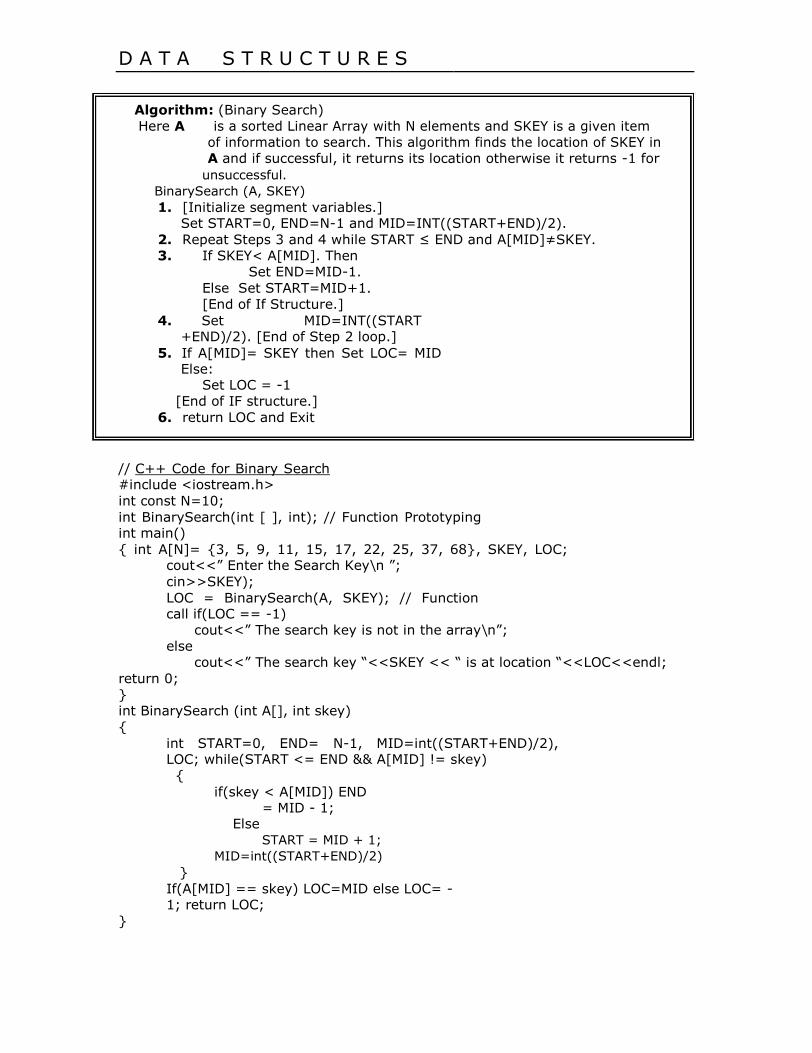
Algorithm: (Binary Search) Here A is a sorted Linear Array with N elements and SKEY is a given item

of information to search. This algorithm finds the location of SKEY in A and if successful, it returns its location otherwise it returns -1 for

unsuccessful.

BinarySearch (A, SKEY) 1. [Initialize segment variables.]

Set START=0, END=N-1 and MID=INT((START+END)/2). 2. Repeat Steps 3 and 4 while START ≤ END and A[MID]≠SKEY. 3. If SKEY< A[MID]. Then

Set END=MID-1. Else Set START=MID+1. [End of If Structure.]

4. Set MID=INT((START +END)/2). [End of Step 2 loop.]

5. If A[MID]= SKEY then Set LOC= MID Else:

Set LOC = -1

[End of IF structure.] 6. return LOC and Exit

// C++ Code for Binary Search #include <iostream.h> int const N=10; int BinarySearch(int [ ], int); // Function Prototyping int main() { int A[N]= {3, 5, 9, 11, 15, 17, 22, 25, 37, 68}, SKEY, LOC;

cout<<” Enter the Search Key\n ”; cin>>SKEY); LOC = BinarySearch(A, SKEY); // Function call if(LOC == -1)

cout<<” The search key is not in the array\n”;

else

cout<<” The search key “<<SKEY << “ is at location “<<LOC<<endl; return 0; }

int BinarySearch (int A[], int skey)

{ int START=0, END= N-1, MID=int((START+END)/2), LOC; while(START <= END && A[MID] != skey) {

if(skey < A[MID]) END = MID - 1;

Else START = MID + 1;

MID=int((START+END)/2) }

If(A[MID] == skey) LOC=MID else LOC= -1; return LOC;

}

D A T A S T R U C T U R E S Computational Complexity of Binary Search

The Computational Complexity of the Binary Search algorithm is measured

by the maximum (worst case) number of Comparisons it performs for searching operations. The searched array is divided by 2 for each comparison/iteration. Therefore, the maximum number of comparisons is measured

by: log2(n) where n is the size of the array Example:

If a given sorted array 1024 elements, then the maximum number of comparisons required is: log2(1024) = 10 (only 10 comparisons are enough)

Computational Complexity of Linear Search

Note that the Computational Complexity of the Linear Search is the

maximum number of comparisons you need to search the array. As you are visiting all the array elements in the worst case, then, the number of

comparisons required is: n (n is the size of the array)

Example: If a given an array of 1024 elements, then the maximum number of comparisons required is:

n-1 = 1023 (As many as 1023 comparisons may be required)

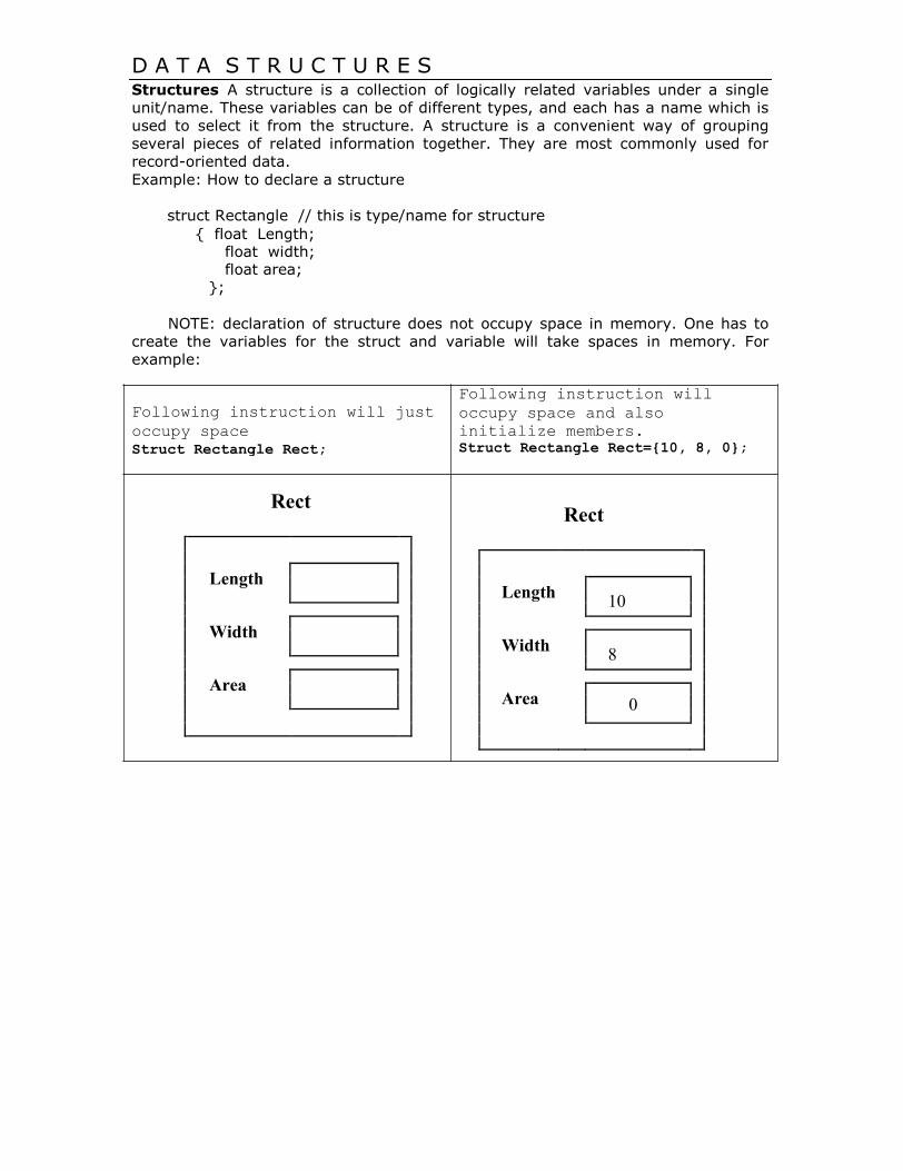
D A T A S T R U C T U R E S Structures A structure is a collection of logically related variables under a single

unit/name. These variables can be of different types, and each has a name which is

used to select it from the structure. A structure is a convenient way of grouping

several pieces of related information together. They are most commonly used for

record-oriented data. Example: How to declare a structure

struct Rectangle // this is type/name for structure { float Length;

float width; float area;

};

NOTE: declaration of structure does not occupy space in memory. One has to

create the variables for the struct and variable will take spaces in memory. For

example:

Following instruction will just Following instruction will

occupy space and also

occupy space initialize members.

Struct Rectangle Rect; Struct Rectangle Rect={10, 8, 0};

Rect Rect

Length

Length

10

Width

Width

8

Area

Area

0