(arrays of structures) and soa (structures of arrays)

1

Case Study

A case study comparing AoS (Arrays of Structures) and SoA

(Structures of Arrays) data layouts for a compute-intensive loop run

on Intel® Xeon® processors and

Intel® Xeon Phi™ product family coprocessors

Abstract

A customer recently purchased a significant number of Intel Xeon Phi coprocessors to augment the

capabilities of their cluster of 16-core dual-socket compute nodes based on the Intel Xeon E5-2600

series processors (with 8 cores per socket). The 61 core Intel Xeon Phi coprocessors can be

programmed to execute natively as a separate Linux* host or via an offload method controlled by

the Intel Xeon processor host. In this case study, we take one mini-application code, tested the host

version, tried out the Intel Xeon Phi coprocessor native execution, optimized the native version (and

as often happens, also the host version) by switching two AoS arrays (“arrays of structures”)

containing three-dimensional point data to the SoA format (“structures of arrays”). We also added

an “offload pragma” to offload the key O(N2) loop, keeping almost all of the performance of the

native version in the offload version. In addition, we did a cache-blocking transformation on the two

main loops by creating 4 loops and then interchanging the two middle (non-inner, non-outer) loops.

Finally we compare the performance of all tested Intel Xeon and Intel Xeon Phi coprocessor versions

showing that a 9 to 1 performance ratio exists between the slowest AoS double precision

executable vs. the fastest SoA single precision executable.

2

Table of Contents

(1) Introduction…………………………………………………………………………………………………………………………….…………………. 2

(2) Two Similar but Very Different Architectures………………………………………………………………………………… 3

(3) Application Benchmark Method Goals.……………………………………………………………………………………………….. 6

(4) Peak Performance View……………………………………………………………………………………………………………..………….. 9

(5) General Vectorization Advice…………………………………………………………………………………………………………………11

(6) Iterative Closest Point Results………………………………………………………………………………………………….………… 12

(7) Detailed Optimization History……………………………………………………………………………………………………………… 17

(8) Assembly Analysis of AoS code vs. SoA code…………………………………………………………………….…….…….. 19

(9) Conclusions………………………………………………………………………………………………………………………….……………………. 28

Introduction

A customer recently purchased a significant number of Intel Xeon coprocessors to augment the

capabilities of their cluster of 16-core dual-socket compute nodes based on Intel Xeon E5-2600

series processors (with 8 cores per socket). They will be supporting a wide variety of software

packages on these systems. They already run clusters with the same set of supported software

packages on earlier x86_64 clusters. Intel has developed software technology in the form of Intel®

compilers, Intel® Math Kernel Library (Intel® MKL), Intel® MPI libraries, and Intel performance analysis

tools that allow this customer and their users to port their software to run natively on the Intel

Xeon Phi coprocessor’s Linux* OS as if it were a separate Linux host or to offload compute tasks

from the host to the Intel Xeon Phi coprocessor located on the PCIe bus of the host.

At this point in time, it has been demonstrated that significant compute server codes (i.e. not client-

based Windows* oriented user-interactive codes) can be ported to or partially offload-enabled for

Intel Xeon Phi coprocessor without a huge amount of software work. However, the remaining task

for a software developer is to “tune & optimize” their software so that it runs efficiently & quickly

on the coprocessor. Intel Xeon is able to run x86_64, 128-bit SSE (Streaming SIMD Extensions),

128-bit AVX-1, or 256-bit AVX-1 (Intel® Advanced Vector Extensions (Intel® AVX) codes using “big

cores” with out-of-order (OOO) capabilities, but the Intel Xeon Phi coprocessor can only run in-order

x86_64 instructions (including x87 instructions) or the new 512-bit Intel® Initial Many Core

Instructions (Intel® IMCI) floating point vector instructions. Ideally, we’d like to develop a decision

tree or step-by-step recipe for software developers to be able to follow in their porting &

optimization activities so that excellent performance can be attained with the minimum amount of

software developer work.

http://legal.intel.com/tmb/Namesdb/search.asp#1999

3

Two Similar but Very Different Architectures

So let’s describe the hardware features that a software developer may want to keep in mind when

programming for the two different architectures: Intel Xeon and Intel Xeon Phi coprocessors. First,

let’s list key attributes of an Intel Xeon E5-2680 compute node (a specific example of the E5-2600

series):

2-sockets with 8 physical cores on each socket for a total of 16 physical cores.

Each physical core can be run as 2 logical cores using Intel® Hyper-Threading Technology

(Intel® HT Technology) if desired by the system administrators who boot up the systems (via

BIOS settings). (This particular HPC customer runs all nodes with Intel HT turned off.)

Intel Xeon & Intel Xeon Phi coprocessors have L1 data caches with 32 kilobytes per core.

Intel Xeon & Intel Xeon Phi coprocessors have L1 instruction caches with 32 kilobytes per

core.

Intel Xeon L2 (combined data/instruction) cache has 256 kilobytes per core.

Xeon E5-2680 L3 cache is 20 Megabytes in size & shared by all 8 cores on a socket for an

average allotment under full use of 2.5 Megabytes per core.

Xeon supports x86_64+x87, Intel® Streaming SIMD Extensions (Intel® SSE) (128-bit), & Intel

AVX-1 (256-bit, 128-bit) instructions

Peak Flops is given by (2.7 GHz)*(16 cores)*(8 DP flops/core) = 345.6 DP GigaFlops (GFs)

With turbo enabled, the peak sustained frequency can be 3.0 GHz, or 384 GF/s.

At 90% efficiency without turbo enabled, Intel Xeon E5-2680 would deliver 311 DP GF/s.

With turbo enabled and latest Intel MKL, Intel Xeon E5-2680 node actually delivers ~345

DGEMM DP-GF/s, which is the peak performance at the base frequency. In other words, the

sustained turbo boost on all cores can offset the efficiency loss so that peak base frequency

performance is achieved for DGEMM. The corresponding SMP Linpack performance is ~330

DP GF/s.

Peak Flops per Core is 21.6 DP GF/s per core. You must be running fully-vectorized, fully-

parallelized cache-blocked code using Intel® AVX with turbo enabled to get near this.

Fully-parallelized cached-blocked scalar apps (e.g. CFD codes) peak at 86.4 DP Gigaflops.

Realizable Stream Bandwidth is approximately 75.2 Gigabytes/second (GB/s) or about 4.7

Gigabytes/sec per core on average. Serial stream bandwidth is measured at 10.4 GB/s.

Ideal Peak Memory Bandwidth is 4 channels/socket*1600 MHz * 2sockets * 8 bytes per

transfer = 102.4 GB/sec. So Xeon achieves 73.4% of the peak memory bandwidth.

Xeon’s 256-bit AVX-1 vector instructions allow 8-floats or 4-doubles operated on at one

time.

Xeon bytes per flop = 75.2 GB/s Stream / 330 Linpack DP-GF/s = 0.23 bytes/flop

4

Next, we list key attributes of an Intel Xeon Phi SE10P coprocessor running at 1.09 GHz [1]:

1-socket with N physical cores: N may vary with SKU; we consider only 61 cores here.

Each physical core is run as 4 logical cores (4-way symmetric multi-threading on Intel Xeon

Phi coprocessor)

Intel Xeon & Intel Xeon Phi coprocessor have L1 data caches with 32 kilobytes per core.

Intel Xeon & Intel Xeon Phi coprocessor have L1 instruction caches with 32 kilobytes per

core.

Intel Xeon Phi coprocessor L2 cache has 512 kilobytes per core (double that of Intel Xeon).

There is no L3 cache at all on Intel Xeon Phi™ coprocessors.

Supports only x86_64+x87 +IMCI (512-bit) instructions (No Intel SSE or Intel AVX-1

support).

Peak Flops is given by (1.09 GHz)*(61 cores)*(16 DP flops/core) = 1064 DP Gigaflops

o At 75.4% Linpack efficiency, this yields 802 realizable Linpack DP GF/s.

o At 83.4% DGEMM efficiency, this yields 885 realizable DGEMM DP/GFs.

Peak flops/core is 17.4 DP GF/s per physical core. Must be running a fully-vectorized fully-

parallelized cache-blocked application using IMCI (512-bit) instructions to achieve this.

Fully-parallelized cache-blocked scalar apps peak at 66.5 DP Gigaflops.

Stream Bandwidth is about 170 Gigabytes/second or about 2.8 Gigabytes/sec per core.

Serial stream bandwidth is measured at about 5.4 GB/s.

Ideal Peak Memory Bandwidth is 8 channels/socket * 5.5 GigaTransfers/sec * 8 bytes per

transfer = 352 GB/sec. Actual stream bandwidth is only 48.3% of the peak memory

bandwidth.

512-bit vector instructions allow 16-float or 8-double IMCI vector instructions.

Intel Xeon Phi coprocessor bytes per flop = 170 GB/s Stream / 802 Linpack DP GF/s = 0.21

bytes/flop

We summarize the above information in the following Table 1 for easy reference.

5

Xeon E5-2680

processor 2.7GHz

Intel Xeon Phi SE10P

coprocessor 1.09 GHz

Sockets 2 1

Physical Cores 16 61

Logical Cores 32 244

L1 Instruction Cache 32k 32k

L1 Data Cache 32k 32k

L2 Cache 256k 512k

L3 Cache 20,000k 0k (None)

x86_64 instructions Yes Yes

x87 instructions Yes Yes

SSE/4floats/2doubles Yes No

AVX-1/8floats/4doubles/NoFMA Yes No

IMCI/16floats/8doubles/FMA No Yes

Peak DP Vector Flops 345.6 GF/s 1063.84 GF/s

Actual (SMP) Linpack Performance 330 GF/s 802 GF/s

Actual DGEMM Performance 347 GF/s 887 GF/s

Peak DP Scalar Flops 86.4 GF/s 66.5 GF/s

Clock Frequency 2.7GHz 1.09GHz

Peak Flops/Physical Core 21.6 GF/s-c 17.4 GF/s-c

Actual Linpack Flops/Physical Core 20.6 GF/s-c 13.1 GF/s-c

Stream Bandwidth 75.2 GB/s 171 GB/s

Average Stream per Core 4.7 GB/s-c 2.6 GB/s-c

Measured Serial Stream 10.4 GB/s-c 5.37 GB/s-c

Peak Mem BW (GB/s) 102.4 GB/s 352 GB/s

Bytes per DP Flop 0.23 b/f 0.21 b/f

Single System Linpack Efficiency 95.5% (turbo on) 75.4%

(Offload) DGEMM Performance (GF/s) 345 GF/s 872 GF/s

Table 1. Comparing Intel Xeon E5-2680 node to Intel Xeon Phi SE10P coprocessor

6

Next we define the “Intel Xeon Phi coprocessor/Intel Xeon-E5” performance Ratio (PXR) as the ratio

of peak or actual performance of the Intel Xeon Phi coprocessor architecture to the peak or actual

performance of the Xeon architecture. Note that the idealized peak PXR ratio (1063.84/345.6) is

3.1x so in general I do not expect to see applications where this performance ratio is greater than

3.1x. If you see a ratio of higher than 3.1x, this would tend to indicate there is some feature or an

issue that needs further explanation. For example, Intel Xeon Phi coprocessor has additional

hardware support for single precision logf( ) and expf( ) functions that Xeon does not have. If we

consider the single-node actual Linpack Intel Xeon Phi coprocessor/Xeon-E5 performance ratio, then

the best value is 2.4x (=802/330).

Application Benchmark Method Goals

The “spectrum” of computing applications is a huge ensemble of software “art” and engineering

created over the past sixty years. A subset of this code ensemble is written in Fortran, C, and C++.

Each “benchmark-able” software package accepts some input and generates some output. More

often than not in today’s world, the input is partially or completely specified by user interaction via a

user interface. However, the command line is still alive and well, and preferred with those who

benchmark software and those in the HPC cluster world. For benchmarking purposes, all the

measurement details can be abstracted to a single command line:

$ measure_time executable_name input_filename

Each executable can have its own “spectrum” of different performance behaviors across the set of

all input files or “workloads” depending on the complexity of the software. Implicit also in each run

of an executable on a workload is (1) the compiler & linker that generated that executable and (2)

the hardware and operating system that the benchmark run was performed on.

Intel Xeon Phi™ coprocessor & Xeon architectures allow software developers to parallelize their

software in hopes that runtimes for a given software package and a given workload will decrease

with the use of more cores. Parallelization (or parallel) speedup P is measured by finding the ratio of

single core runtime to N-core runtime.

P = RunTime(1-core)/RunTime(N-cores) >= 1

This property is easy to measure for OpenMP* executables in that one typically does not have to

recompile source code to measure P. Ideal speedup on N logical cores is N. Superlinear speedup

occurs when P > N. In most cases, we find 1 < P < N. (It is certainly possible for multiple core usage

to slow down the execution of your software; it is way more common than one might think. In those

cases, you should analyze and redesign your application if possible.)

Vectorization technology is technically much different than multiple core technology. Some lump

vectorization and parallelization together into the term “parallelization” because the terms “SIMD

parallelization” and “SIMD vectorization” are both terms for the same underlying idea. Intel products

offer SIMD vectorization features that may or may not be used by any given loop of any given

7

software package. In the author’s experience, users may think they are getting great vector

speedup on today’s Intel Xeon systems, but in general it is not usually true unless, for example, they

are calling the Intel MKL DGEMM function for much of the work of the application.

Intel SSE vectorization (128-bit, 4 float, 2 double) instructions is offered on Intel architecture X5600

series processors and prior. We also now offer Intel AVX-1 vectorization (256-bit, 8 float, 4 double)

instructions on Intel Xeon E3/E5 series & Core processors. And we offer Intel Initial Many Core

Instruction (Intel® IMCI) vectorization (512-bit, 16 float, 8 double) on the Intel Xeon Phi™

coprocessors now available. Later in 2013, AVX-2 instructions that include fused-multiply & add will

be available from Intel.

Intel® Compiler software technology allows one to rebuild executables without using vector or FMA

(fused multiply & add) instructions by using the “-no-vec –no-fma” compiler options. This allows you

to measure the vectorization (or vector) speedup V by finding the ratio of the non-vectorized

runtime to the vectorized runtime at full parallelization:

V = RunTime(No-Vectorization&No-FMA)/Runtime(Full-Vectorization-and-FMA )

Measuring V requires access to source code to achieve recompilation & re-linking. For SSE,

1<=V<=4 for single precision and 1<V<2 for double precision. For AVX-1, 1<=V<=8 for single

precision and 1<V<4 for double precision. For Intel Xeon Phi coprocessor, 1<=V<=16 for single and

1<V<8 for double precision. This is summarized in Table 2.

Instructions Single

Precision Double

Precision

SSE 4 (No FMA) 2 (No FMA)

AVX-1 8 (No FMA) 4 (No FMA)

AVX-2 8 (FMA) 4 (FMA)

IMCI 16 (FMA) 8 (FMA)

Table 2: Number of Vector Elements for Single & Double Precision Vector Instructions

Intel Xeon & Intel Xeon Phi coprocessor architectures have different properties as noted in Tables 1

& 2. However, if V(Xeon,SSE) = V(Xeon, AVX-1) = ~1, it is not likely that V will be much greater

than 1 on Intel Xeon Phi coprocessor. If V(Intel Xeon Phi coprocessor) >> 1, then V(Xeon,SSE) and

V(Xeon,AVX-1) will likely be (much) greater than one in typical situations. In qualitative terms, the

Intel Xeon Phi coprocessor architecture can act as a “vectorization performance amplifier.” In fact,

developers optimizing for Intel Xeon Phi coprocessors often find that the same source code is also

better optimized for Intel Xeon host processors. One way to state this without implying a specific

cause and effect relationship is to state that for a given software package auto-vectorized by Intel®

compilers:

Vector Speedup on Intel Xeon Phi™ coprocessor & Vector Speedup on

Intel Xeon are strongly correlated.

From a basic multivariate optimization perspective, if one wants to optimize the parallel speedup P

and the vector speedup V, it would make sense to define an objective function B=P*V that one

8

would jointly optimize in order to optimize a given application. We will next argue that this choice of

objective function for evaluating application performance is very natural and has a “Linpack-ness”

quality to it.

Switching gears for the moment, the Top500 List ranks interconnected computing systems by their

Rmax scores, measured today in PetaFlops. Rmax is always less than or equal to Rpeak. How are

these values defined and measured? First we define Rpeak of a given node as the following:

Rpeak = P_ideal*V_ideal*F

where F is the clock frequency of the compute node, V_ideal is the ideal vector speedup (including

effects of FMA (fused multiply & add) and/or multiple op retirements), and P_ideal is the ideal

parallel speedup, or the number of physical cores. When HPL LINPACK code is run on a given node

or cluster of nodes, the value Rmax is obtained. Rmax is always less than Rpeak. The LINPACK

efficiency E is defined at the ratio of the maximum measured performance to the peak performance

and is often expressed as a percentage:

E = Rmax/Rpeak

So we might also write this as

Rmax = E* P_ideal*V_ideal*F .

Values of E can run anywhere from lower fractions up to 95% or more depending upon the

hardware architecture. The value of E accounts for all the non-ideal-ness of the best LINPACK run.

The only thing we are proposing above that is not usually done is to break efficiency into two terms:

parallelization efficiency and vectorization efficiency.

E = E_par * E_vec

We can then regroup the above equation into

Rmax = (E_par* P_ideal) * (E_vec*V_ideal) * F

= (P_measured) * (V_measured) * F

where

E_par = P_measured / P_ideal

E_vec = V_measured / V_ideal

For most other real application benchmarks besides Linpack and Matrix Multiplication (aka DGEMM /

SGEMM), we seldom see Flops (floating point operations per second) values getting so close to

Rpeak. But we’d like to be able to rank applications by their ability to make use of multiple cores and

vector units simultaneously. Therefore, we measure P at full vectorization & optimization and we

measure V at full parallelization (but with no-vec and no-fma used) and define a ranking metric B

9

that quantifies the given application (and workload)’s ability to take advantage of the Intel hardware

that it is running on:

B = P_measured * V_measured (= Rmax/F)

Bpeak = Rpeak/F

So any software application S with a workload W can be measured on a given architecture A having

used compiler/linker C to give a value B(S,W,A,C) which should range in value from 1 to Bpeak. High

B values on Intel Xeon correlate with high B values on the Intel Xeon Phi coprocessor and vice versa.

Low B values on Intel Xeon correlate with low B values on Intel Xeon Phi coprocessors.

In Figure 1 below, we show Vector Speedup and Parallel Speedup and Combined Vector-Parallel

Speedup for N operations of work to be done. A simple 2x2 table summarizes the possible

speedups.

Figure 1. 2x2 Table showing Vector & Parallel Speedup Factors

At this point, the reader should understand this simple framework to measure multi-core

parallelization effectiveness and SIMD vectorization effectiveness together that is relevant to any

application. A serial non-vectorized code (most software) will have B =1. Software can speedup

with vector speedup or parallel speedup or both as shown in Figure 1.

10

Peak Performance View

As James Reinders has pointed out in his recent paper [2], it is helpful to look at a plot of GigaFlops

versus thread count for Intel Xeon and Intel Xeon Phi processors. We could plot measured data for

all lines shown, but it is easier for discussion to look at peak performance functions for each line of

interest. If T=ThreadCount and Gigaflops(label, T)=Peak Gigaflops for the “label”

architecture/software configuration, then we can compare the following functions:

(1) Gigaflops(XeonE5-2680_AVX1,T) = 2.7*8*T = 21.6*T

(2) Gigaflops (XeonE5-2680_SSE,T) = 2.7*4*T = 10.8*T

(3) Gigaflops (XeonE5-2680_NoVec,T) = 2.7*2*T = 5.4*T

(4) Gigaflops (Phi_FullVec,T) = 1.09*4*T = 4.36*T

(5) Gigaflops (Phi_NoVec,T) = 1.09*0.25*T = 0.2725*T

(6) Gigaflops (Phi_DGEMM,T) = 1.09*3.335*T = 3.635*T

(7) Gigaflops (Phi_Linpack,T) = 1.09*3.015*T = 3.287*T

Note that G(Phi_NoVec,T=244) = 66.49 which is less than G(XeonE5-2680_NoVec,T=16) = 86.4.

This means that if a code yields no vector speedup (no auto-vectorization that produces speedup) at

all, then it is not very likely that Xeon Phi will ever exceed the performance of Intel Xeon even if it

is fully parallel. That is, “highly parallel” is not enough to allow Phi to provide benefit in most cases.

Note also that G(Phi_FullVec,1) = 4.36 which is less than G(XeonE5-2680_NoVec,1) = 5.4. This

means that a fully vectorized single thread on Xeon Phi cannot beat the performance of a single

thread on Intel Xeon even if the app is not parallel and not vectorized on Intel Xeon.

Taken all together this means that an application (or hot loop of an application) will have to scale to

at least 2 threads per physical Xeon Phi core and be very well vectorized in order to do better than

Intel Xeon. All the statements just made and the linear functions mentioned above are shown in

Figure 2 below.

11

Figure 2. Peak GigaFlops as a function of Thread Count (Intel Xeon-E5-2680 & Intel Xeon Phi SE10P)

General Vectorization Advice

So we’ll start out this section with the claim that most software (>~85%) is not “well vectorized” in

that it has very low vector speedup V when measured (approximately 1.0). Part of the reason for

this is that some apps and some hot loops are doing work that is not able to be vectorized for

mathematical dependency reasons. We refer to software portions in this category as “inherently

non-vectorizable (INV).” We do not have an estimate for how much of the software that has “low

vector speedup (LVS)” is also in the category “inherently non-vectorizable (INV)” but it is not small.

The set relationships are shown graphically in Figure 3 below. The shaded region is the region of

candidate applications for Xeon Phi™. The set relationship is written mathematically using subset

notation as the following:

INV LVS All Software

12

Figure 3. Subset relationships of various types of software. Software in the blue region is eligible to

be considered for implementation on Intel Xeon Phi™.

In this section, we describe some relatively simple ways to get the Intel® ComposerXE compiler to

vectorize code that is outside the INV class but inside the LVS class (without using intrinsics).

Suppose you have a “hot” loop that you think should vectorize but it’s not vectorizing (as discovered

in Vtune, SDE or other hot loop tool). Then try basic auto-vectorization first by using the appropriate

compiler options (or “knobs”). Use “-vec-report2” or higher for debug information about whether or

not loops are vectorizing. To ask for AVX auto-vectorization for Intel Xeon E5-2680 you use the

compiler command line option “-xAVX –O3”. To ask for Xeon Phi auto-vectorization for Intel Xeon

Phi native executables, you use the compiler command line option “-mmic –O3”. Offload compilation

should give you –mmic auto-vectorization in general, but you can use the host compiler option -

offload-option,compiler,mic,” “ to pass any additional options to the Xeon Phi compiler if needed.

Other things to try include the following:

1. Try “#pragma vector always” to disable the compiler’s vectorization cost model. Always

check for performance after introducing this option. The main thing you need to know is

that the vectorizer uses heuristics. Heuristics by definition are not always correct.

2. Try “#pragma ivdep” if you know there are no true dependences that should prevent

vectorization. Always check for correctness and possible crashes after introducing this

option.

3. Try “#pragma simd.” If neither of the above work to give you vectorized code, then try this

option. Always check for performance, correctness, & possible crashes after introducing this

option.

Don’t forget to “check your work” by examining assembly with compiler –S option and cross-

checking to your source code line numbers. “Examining assembly” may sound like a tall order if

you’ve never written assembly, but if you’ve read this far in this paper, you may find that you can

13

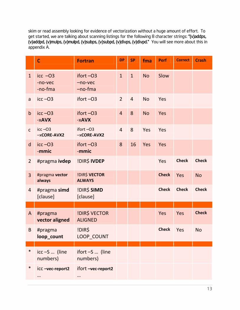
skim or read assembly looking for evidence of vectorization without a huge amount of effort. To

get started, we are talking about scanning listings for the following 8 character strings: “(v)addps,

(v)addpd, (v)mulps, (v)mulpd, (v)subps, (v)subpd, (v)divps, (v)divpd.” You will see more about this in

appendix A.

C Fortran DP SP fma Perf Correct Crash

1 icc –O3 -no-vec -no-fma

ifort –O3 –no-vec –no-fma

1 1 No Slow

a icc –O3 ifort –O3 2 4 No Yes

b icc –O3 -xAVX

ifort –O3 -xAVX

4 8 No Yes

c icc –O3 –xCORE-AVX2

ifort –O3 –xCORE-AVX2

4 8 Yes Yes

d icc –O3 -mmic

ifort –O3 -mmic

8 16 Yes Yes

2 #pragma ivdep !DIR$ IVDEP Yes Check Check

3 #pragma vector always

!DIR$ VECTOR ALWAYS

Check Yes No

4 #pragma simd [clause]

!DIR$ SIMD [clause]

Check Check Check

A #pragma

vector aligned !DIR$ VECTOR ALIGNED

Yes Yes Check

B #pragma loop_count

!DIR$ LOOP_COUNT

Check Yes No

* icc –S … (line

numbers) ifort –S … (line numbers)

* icc –vec-report2

… ifort –vec-report2

…

14

Vectorization Recommendations:

• Find your hot loops/hot basic blocks first (Vtune, SDE, …)

• Make sure your arrays are aligned (if possible)

• Make sure you don’t have bad dependencies (i.e. algorithm is vectorizable)

• Try auto-vectorization first e.g. with

• Options: –O3 –xAVX –vec-report2 –openmp

• Analyze why the compiler wasn’t able to vectorize Then try: #pragma vector always

• Then try: #pragma ivdep

• Use: #pragma vector aligned if the compiler is not noticing that your arrays are aligned.

• Then try: #pragma simd: It will usually vectorize if it is a vectorizable loop.

– Forces vectorization regardless of safety: Check for correctness & test thoroughly

• Consult compiler’s –S assembly listing on regular basis as you work

– Be patient with yourself…this will become easier fairly quickly.

• Any vectorizable algorithm should permit Fortran or C vectorizable loop implementation that

will work with !DIR$SIMD or #pragma simd

– You may need to flag reduction operations specifically as such

• Help compiler with #pragma loop_count if you know your trip counts (loop counts).

• Test #pragma unroll(N) around loops to see if it helps performance.

• You must vectorize for Intel Xeon Phi. Don’t think that you are not going to have to worry

about vectorization in order to get real performance on Intel Xeon Phi. (Some may point out

that Stream achieves a significant portion of its peak performance without vectorization so

your application might too, touting the high memory bandwidth on the card.)

Iterative Closest Point Results

Next we’ll use the ICP (Iterative Closest Point) benchmark application available with this paper [3].

ICP is a fundamental 3d shape matching algorithm described in [4]. The ICP benchmark is a relatively

simple 500 line program which does a brute force O(N^2) implementation of the ICP algorithm.

Because of the simplicity of the program, we can measure not only single and double precision

results but also Structure of Arrays (SoA) and Arrays of Structures (AoS) performance very easily

just using some C preprocessor definitions.

The “infrastructure” for this testing is pretty trivial and controlled via compile line options:

#if defined(AOS)

#define AOSFLAG 1 // 1 for AoS

#else

#define AOSFLAG 0 // 0 for SoA (default)

#endif

#if defined(DOUBLEPREC)

#define FPPRECFLAG 2 // 2 for Double precision

#define FLOATINGPTPRECISION double

#else

#define FPPRECFLAG 1 // 1 for Single precision (default)

#define FLOATINGPTPRECISION float

#endif

15

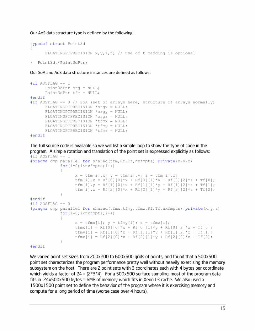
Our AoS data structure type is defined by the following: typedef struct Point3d

{

FLOATINGPTPRECISION x,y,z,t; // use of t padding is optional

} Point3d,*Point3dPtr;

Our SoA and AoS data structure instances are defined as follows: #if AOSFLAG == 1

Point3dPtr org = NULL;

Point3dPtr tfm = NULL;

#endif

#if AOSFLAG == 0 // SoA (set of arrays here, structure of arrays normally)

FLOATINGPTPRECISION *orgx = NULL;

FLOATINGPTPRECISION *orgy = NULL;

FLOATINGPTPRECISION *orgz = NULL;

FLOATINGPTPRECISION *tfmx = NULL;

FLOATINGPTPRECISION *tfmy = NULL;

FLOATINGPTPRECISION *tfmz = NULL;

#endif

The full source code is available so we will list a simple loop to show the type of code in the

program. A simple rotation and translation of the point set is expressed explicitly as follows: #if AOSFLAG == 1

#pragma omp parallel for shared(tfm,Rf,Tf,nxfmpts) private(x,y,z)

for(i=0;i<nxfmpts;i++)

{

x = tfm[i].x; y = tfm[i].y; z = tfm[i].z;

tfm[i].x = Rf[0][0]*x + Rf[0][1]*y + Rf[0][2]*z + Tf[0];

tfm[i].y = Rf[1][0]*x + Rf[1][1]*y + Rf[1][2]*z + Tf[1];

tfm[i].z = Rf[2][0]*x + Rf[2][1]*y + Rf[2][2]*z + Tf[2];

}

#endif

#if AOSFLAG == 0

#pragma omp parallel for shared(tfmx,tfmy,tfmz,Rf,Tf,nxfmpts) private(x,y,z)

for(i=0;i<nxfmpts;i++)

{

x = tfmx[i]; y = tfmy[i]; z = tfmz[i];

tfmx[i] = Rf[0][0]*x + Rf[0][1]*y + Rf[0][2]*z + Tf[0];

tfmy[i] = Rf[1][0]*x + Rf[1][1]*y + Rf[1][2]*z + Tf[1];

tfmz[i] = Rf[2][0]*x + Rf[2][1]*y + Rf[2][2]*z + Tf[2];

}

#endif

We varied point set sizes from 200x200 to 600x600 grids of points, and found that a 500x500

point set characterizes the program performance pretty well without heavily exercising the memory

subsystem on the host. There are 2 point sets with 3 coordinates each with 4 bytes per coordinate

which yields a factor of 24 = (2*3*4). For a 500x500 surface sampling, most of the program data

fits in 24x500x500 bytes = 6MB of memory which fits in Xeon L3 cache. We also used a

1500x1500 point set to define the behavior of the program where it is exercising memory and

compute for a long period of time (worse case over 4 hours).

16

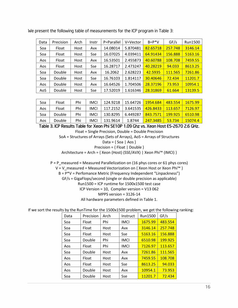
We present the following table of measurements for the ICP program in Table 3:

Data Precision Arch Instr P=Parallel V=Vector B=P*V GF/s Run1500

Soa Float Host Avx 14.08014 5.870481 82.65718 257.748 3146.14

Soa Float Host Sse 16.07025 4.039411 64.91434 156.888 5163.16

Aos Float Host Avx 16.53501 2.455873 40.60788 108.708 7459.55

Aos Float Host Sse 16.28717 2.473247 40.28219 94.033 8613.25

Soa Double Host Avx 16.2062 2.628223 42.5935 111.565 7261.86

Soa Double Host Sse 16.76103 1.814117 30.40646 72.434 11201.7

Aos Double Host Avx 16.64526 1.704506 28.37196 73.953 10954.1

AoS Double Host Sse 17.52019 1.616346 28.31869 61.664 13139.5

Soa Float Phi IMCI 124.9218 15.64726 1954.684 483.554 1675.99

Aos Float Phi IMCI 117.2152 3.641535 426.8433 113.657 7126.97

Soa Double Phi IMCI 130.8295 6.449287 843.7571 199.925 6510.98

Aos Double Phi IMCI 131.9614 1.8744 247.3485 53.734 15074.4

Table 3. ICP Results Table for Xeon Phi SE10P 1.09 Ghz vs. Xeon Host E5-2670 2.6 GHz. Float = Single Precision, Double = Double Precision

SoA = Structures of Arrays (Sets of Arrays), AoS = Arrays of Structures Data = { Soa | Aos }

Precision = { Float | Double } Architecture = Arch = { Xeon (Host) (SSE/AVX) | Xeon Phi™ (IMCI) }

P = P_measured = Measured Parallelization on (16 phys cores or 61 phys cores)

V = V_measured = Measured Vectorization on { Xeon Host or Xeon Phi™ } B = P*V = Perfomance Metric (Frequency Independent “Linpackness”)

GF/s = GigaFlops/second (single or double precision as applicable) Run1500 = ICP runtime for 1500x1500 test case ICP Version = 10, Compiler version = V13 062

MPPS version = 3126-14 All hardware parameters defined in Table 1.

If we sort the results by the RunTime for the 1500x1500 problem, we get the following ranking:

Data Precision Arch Instruct Run1500 GF/s

Soa Float Phi IMCI 1675.99 483.554

Soa Float Host Avx 3146.14 257.748

Soa Float Host Sse 5163.16 156.888

Soa Double Phi IMCI 6510.98 199.925

Aos Float Phi IMCI 7126.97 113.657

Soa Double Host Avx 7261.86 111.565

Aos Float Host Avx 7459.55 108.708

Aos Float Host Sse 8613.25 94.033

Aos Double Host Avx 10954.1 73.953

Soa Double Host Sse 11201.7 72.434

17

AoS Double Host Sse 13139.5 61.664

Aos Double Phi IMCI 15074.4 53.734

Table 4. Performance Ranking for case N=1500 runs for Different Versions on

Intel® Xeon and Intel Xeon Phi

(Fastest/Slowest Ratio: 9 to 1)

In what follows we use the symbol ‘>’ to indicate that the performance of the left side executable is

faster/better than the performance of the right side executable. We draw the following conclusions

for this ICP application benchmark:

SoA is better than AoS on “Intel Xeon Phi and Intel Xeon_E5-2680 for both Single and Double

Precision Phi Single-precision SoA > Phi Single Precision AoS by a factor of ~4.2x = 7126.97/1675.99

Phi Double-precision SoA > Phi Double Precision AoS by a factor of ~2.3x = 15074.4/6510.98

Xeon Single-precision SoA > Xeon Single Precision AoS by a factor of ~2.4x = 7459.55/3146.14

Xeon Double-precision SoA > Xeon Double Precision AoS by a factor of ~1.5x = 10954.1/7261.86

Intel Xeon Phi SoA better than Intel Xeon_E5-2680 SoA for both Single and Double Precision. Phi Single-precision SoA > Xeon Single-precision SoA by a factor of ~1.88x = 3146.14/1675.99

Phi Double-precision SoA > Xeon Double-precision SoA by a factor of ~1.11x = 7261.86/6510.98

Intel Xeon Phi AoS better than Intel Xeon_E5-2680 AoS for Single Precision Phi Single-precision AoS > Xeon Single-precision AoS by a factor of ~1.05 = 7459.55/7126.97

Intel Xeon_E5-2580 AoS better than Intel Xeon Phi AoS for Double Precision Xeon Double-precision AoS > Phi Double-precision AoS by a factor of ~1.38x = 15074.4/10954.1

The properties of this code that help this happen with the source for this app are the following:

(1) Stride-1 accesses occur for almost all reads & writes.

(2) All arrays are 64-byte aligned & the compiler knows they are 64-byte aligned.

(3) The compiler successfully vectorized all the hot loops.

(4) Loops are Cache-Blocked to reduce memory accesses.

(5) There is no division in the main loop.

(6) Loops are very simple.

In order to understand why SoA is doing better than AoS, let’s look at the assembly language output

for the key loop of the application. It is helpful to understand first how really simple the main loop is.

Several transformations of the loop took place over the history of optimizing this code for Xeon Phi

and some of the transformations are not exactly obvious. So we discuss those first and then move

on to the assembly language discussion.

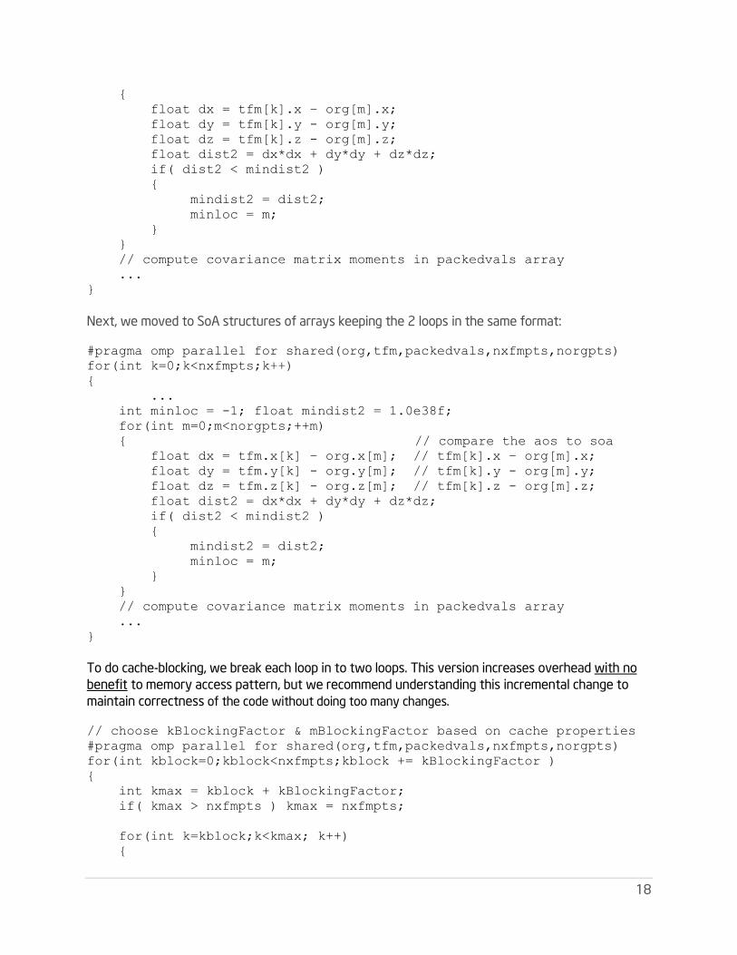
Detailed Optimization History for Basic ICP

First, we started with 2 loops and an AoS array of xyz point coordinate structures.

#pragma omp parallel for shared(org,tfm,packedvals,nxfmpts,norgpts)

for(int k=0;k<nxfmpts;k++)

{

...

int minloc = -1; float mindist2 = 1.0e38f;

for(int m=0;m<norgpts;++m)

18

{

float dx = tfm[k].x – org[m].x;

float dy = tfm[k].y - org[m].y;

float dz = tfm[k].z - org[m].z;

float dist2 = dx*dx + dy*dy + dz*dz;

if( dist2 < mindist2 )

{

mindist2 = dist2;

minloc = m;

}

}

// compute covariance matrix moments in packedvals array

...

}

Next, we moved to SoA structures of arrays keeping the 2 loops in the same format:


for(int k=0;k<nxfmpts;k++)

{

...


for(int m=0;m<norgpts;++m)

{ // compare the aos to soa

float dx = tfm.x[k] – org.x[m]; // tfm[k].x – org[m].x;

float dy = tfm.y[k] - org.y[m]; // tfm[k].y - org[m].y;

float dz = tfm.z[k] - org.z[m]; // tfm[k].z - org[m].z;



{

mindist2 = dist2;

minloc = m;

}

}


...

}

To do cache-blocking, we break each loop in to two loops. This version increases overhead with no

benefit to memory access pattern, but we recommend understanding this incremental change to

maintain correctness of the code without doing too many changes.

// choose kBlockingFactor & mBlockingFactor based on cache properties


for(int kblock=0;kblock<nxfmpts;kblock += kBlockingFactor )

{

int kmax = kblock + kBlockingFactor;

if( kmax > nxfmpts ) kmax = nxfmpts;

for(int k=kblock;k<kmax; k++)

{

19

...


for(int mblock=0;mblock<norgpts;mblock += mBlockingFactor)

{

int mmax = mblock + mBlockingFactor;

if( mmax > norgpts ) mmax = norgpts;

for(int m=mblock; m<mmax; m++ )

{

float dx = tfm.x[k] – org.x[m];

float dy = tfm.y[k] - org.y[m];

float dz = tfm.z[k] - org.z[m];



{

mindist2 = dist2;

minloc = m;

}

} // end of m loop

} // end of mblock loop


...

} // end of k loop

} // end of k block loop

The next step of cache-blocking is to do loop interchange. In this case of the ICP algorithm, we need

additional information so we have to introduce additional arrays to keep track of the minloc[ ] and

mindist2[ ] values.

// choose kBlockingFactor & mBlockingFactor based on cache properties

// initialize minkloc[:]= -1 array and minkdist2[:]= 1.0e38f array


for(int kblock=0;kblock<nxfmpts;kblock += kBlockingFactor )

{

int kmax = kblock + kBlockingFactor;

if( kmax > nxfmpts ) kmax = nxfmpts;

for(int mblock=0;mblock<norgpts;mblock += mBlockingFactor)

{

int mmax = mblock + mBlockingFactor;

if( mmax > norgpts ) mmax = norgpts;


{

int minloc = minkloc[k];

float mindist2 = minkdist2[k];

for(int m=mblock; m<mmax; m++ )

{

float dx = tfm.x[k] – org.x[m];

float dy = tfm.y[k] - org.y[m];

20

float dz = tfm.z[k] - org.z[m];



{

mindist2 = dist2;

minloc = m;

}

} // end of m loop

minkloc[k] = minloc;

minkdist2[k] = mindist2;

} // end of k loop

} // end of m block loop



{

...

} // end of k loop

} // end of k block loop

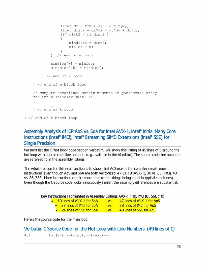
Assembly Analysis of ICP AoS vs. Soa for Intel AVX-1, Intel® Initial Many Core

Instructions (Intel® IMCI), Intel® Streaming SIMD Extensions (Intel® SSE) for

Single Precision

We next list the C “hot loop” code section verbatim. We show this listing of 49 lines of C around the

hot loop with source code line numbers (e.g. available in the VI editor). The source code line numbers

are referred to in the assembly listings.

The whole reason for this next section is to show that AoS makes the compiler create more

instructions even though AoS and SoA are both vectorized: 47 vs. 19 (AVX-1), 38 vs. 23 (IMCI), 48

vs. 26 (SSE). More instructions require more time (other things being equal in typical conditions).

Even though the C source code looks innocuously similar, the assembly differences are substantial.

Key Instructions Highlighted in Assembly Listings AVX-1 (10), IMCI (8), SSE (10)

19 lines of AVX-1 for SoA vs. 47 lines of AVX-1 for AoS

23 lines of IMCI for SoA vs. 38 lines of IMCI for AoS

26 lines of SSE for SoA vs. 48 lines of SSE for AoS

Here’s the source code for the main loop:

Verbatim C Source Code for the Hot Loop with Line Numbers (49 lines of C)

484 for(int k=kblock;k<kmax;k++)

21

485 {

486 FLOATINGPTPRECISION micdist2;

487 FLOATINGPTPRECISION micmindist2;

488 FLOATINGPTPRECISION xmic,ymic,zmic;

489 int micminjloc;

490

491 #if AOSFLAG == 1

492 xmic = tfm[k].x; ymic = tfm[k].y; zmic = tfm[k].z;

493 #endif


495 xmic = tfmx[k]; ymic = mictfmy[k]; zmic = mictfmz[k];

496 #endif

497

498 micminjloc = minkLoc[k];

499 micmindist2 = minkDist2[k];

500

501 #pragma vector aligned

502 #ifdef __MIC__

503 #pragma unroll(0)

504 #endif

505 #ifndef __MIC__

506 #pragma unroll(4)

507 #endif

508 for(int m=mblock;m<mmax;++m)

509 {

510 FLOATINGPTPRECISION micdx,micdy,micdz;


512 micdx = xmic - org[m].x;

513 micdy = ymic - org[m].y;

514 micdz = zmic - org[m].z;

515 #endif


517 micdx = xmic - orgx[m];

518 micdy = ymic - micorgy[m];

519 micdz = zmic - micorgz[m];

520 #endif

521 micdist2 = micdx*micdx + micdy*micdy + micdz*micdz;

522 if( micdist2 < micmindist2 )

523 {

524 micmindist2 = micdist2;

525 micminjloc = m;

526 }

527 } // end of the m loop

528

529 minkLoc[k] = micminjloc;

530 minkDist2[k] = micmindist2;

531

532 } // end of the k loop

22

Intel AVX Assembly: Packed Single (PS) Vectorized Floating Point Summary

(10)

In order to facilitate understanding the assembly generated by the compiler for the given C source

code, we first list the key instructions that you will find when skimming through the output of the

compiler generated using the –S option. We show here the C statement that generated the given

vector instruction as a C comment:

(1) vsubps // float dx = tfm.x[k] – org.x[m];

(2) vsubps // float dy = tfm.y[k] - org.y[m];

(3) vsubps // float dz = tfm.z[k] - org.z[m];

(4) vmulps // dxsquared = dx*dx

(5) vmulps // dysquared = dy*dy

(6) vmulps // dzsquared = dz*dz

(7) vaddps // dist2 = dxsquared + dysquared;

(8) vaddps // dist2 += dzsquared;

(9) vcmpltps // if( dist2 < mindist2 )

(10) vminps // mindist2 = dist2;

Intel IMCI Assembly: Packed Single (PS) Vectorized Floating Point Summary (8)

Similarly we show the IMCI (Initial Many Core Instructions) for the same code. Note that IMCI

contains FMA instructions.

(1) vsubps // float dx = tfm.x[k] – org.x[m];

(2) vsubps // float dy = tfm.y[k] - org.y[m];

(3) vsubps // float dz = tfm.z[k] - org.z[m];

(4) vmulps // dxsquared = dx*dx

(5) vfmadd213ps // dist2 = dy*dy + dxsquared

(6) vfmadd213ps // dist2 = dz*dz + dist2

(7) vcmpltps // if( dist2 < mindist2 )

(8) vgminps // mindist2 = dist2;

Intel SSE Assembly: Packed Single (PS) Vectorized Floating Point Summary (10)

Finally, since SSE has been with us for many years while AVX-1 and IMCI are both new, we also list

the primary SSE instructions generated by the C loop. Note there are 10 key instructions for both

AVX-1 and SSE while IMCI only has 8 key instructions owing to FMA (fused multiply & add) on Xeon

Phi.

(1) subps // float dx = tfm.x[k] – org.x[m];

(2) subps // float dy = tfm.y[k] - org.y[m];

(3) subps // float dz = tfm.z[k] - org.z[m];

(4) mulps // dxsquared = dx*dx

(5) mulps // dysquared = dy*dy

(6) mulps // dzsquared = dz*dz

(7) addps // dist2 = dxsquared + dysquared;

(8) addps // dist2 += dzsquared;

(9) cmpltps // if( dist2 < mindist2 )

(10) minps // mindist2 = dist2;

23

Assembly of Hotspot for Single Precision Intel AVX Structure of Arrays (19

lines)

The process is manual and error-prone, but I’ve selected the actual assembly language text from

the .s file generated using the –S option. You’ll notice that each selection begins with an ‘lea’

instruction (load-effective-address) and ends with a ‘jb’ instruction that is labeled as an 82%

probability. As above we start with the AVX-1 code first. Note this first selection is the SoA code.

Please note how short it is. Note that each statement is doing real work, not just getting ready to do

real work.

lea (%r10,%r14), %r15d #517.26

addl $8, %r14d #508.7

vsubps (%rdi,%r15,4), %ymm0, %ymm13 #517.26

vsubps (%r8, %r15,4), %ymm2, %ymm14 #518.23

vsubps (%rsi,%r15,4), %ymm4, %ymm15 #519.23

vmulps %ymm13, %ymm13, %ymm13 #521.22



vaddps %ymm14, %ymm13, %ymm13 #521.36


vcmpltps %ymm10, %ymm13, %ymm14 #522.20

vminps %ymm10, %ymm13, %ymm10 #522.20

vextractf128 $1, %ymm14, %xmm15 #522.20

vpblendvb %xmm14, %xmm3, %xmm8, %xmm8 #498.7

vpaddd %xmm12, %xmm3, %xmm3 #498.7



cmpl %ebx, %r14d #508.7

jb ..B1.111 # Prob 82% #508.7

Assembly of Hotspot for Single Precision AVX Array of Structures (47 lines)

Now we follow with the AoS assembly code. Note the presence of the “vinsertps” and “vinsertf128”

and “vextract128” instructions which you do not find in the SoA version above.

lea (%rbx,%r14), %r15d #512.26

addl $8, %r14d #508.7

shlq $4, %r15 #512.26

vmovss (%r15,%r8), %xmm15 #512.26

vinsertps $16, 16(%r15,%r8), %xmm15, %xmm14 #512.26

vmovss 64(%r15,%r8), %xmm15 #512.26






vmovss 4(%r15,%r8), %xmm0 #513.26

vinsertf128 $1, %xmm15, %ymm1, %ymm14 #512.26


vsubps %ymm14, %ymm3, %ymm1 #512.26

24


vmovss 68(%r15,%r8), %xmm15 #513.26





vmovss 8(%r15,%r8), %xmm15 #514.26






vmovss 72(%r15,%r8), %xmm15 #514.26











vcmpltps %ymm13, %ymm15, %ymm0 #522.20

vminps %ymm13, %ymm15, %ymm13 #522.20

vextractf128 $1, %ymm0, %xmm1 #522.20





cmpl %eax, %r14d #508.7

jb ..B1.182 # Prob 82% #508.7

Assembly Analysis for Single Precision IMCI Structure of Arrays (SoA) (23 lines)

This is the SoA Intel IMCI assembly. Note the ‘vprefetch’ statements that you do not find in the Intel

AVX-1 or Intel SSE listings.

lea (%rdx,%r14), %r13d #517.26 c1

addl $16, %r14d #508.7 c1

vsubps (%r12,%r13,4), %zmm6, %zmm10 #518.23 c5

lea 128(%r15), %edi #517.26 c5

vsubps (%rsi,%r13,4), %zmm7, %zmm12 #517.26 c9

vprefetch1 (%rsi,%rdi,4) #517.26 c9

vmulps %zmm10, %zmm10, %zmm11 #521.36 c13

vsubps (%r9,%r13,4), %zmm5, %zmm13 #519.23 c17

lea 32(%r15), %r13d #517.26 c17

vfmadd213ps %zmm11, %zmm12, %zmm12 #521.36 c21

vprefetch0 (%rsi,%r13,4) #517.26 c21


vprefetch1 (%r12,%rdi,4) #518.23 c25

vcmpltps %zmm8, %zmm13, %k2 #522.20 c29

25

vprefetch0 (%r12,%r13,4) #518.23 c29

vmovaps %zmm3, %zmm9{%k2} #498.7 c33

vprefetch1 (%r9,%rdi,4) #519.23 c33

addl $16, %r15d #508.7 c37

vprefetch0 (%r9,%r13,4) #519.23 c37

vgminps %zmm8, %zmm13, %zmm8 #522.20 c41

cmpl %r8d, %r14d #508.7 c41

vpaddd %zmm4, %zmm3, %zmm3 #498.7 c45

jb ..B1.120 # Prob 82% #508.7 c45

Assembly Analysis for Single Precision IMCI Array of Structures (AoS) (38 lines)

This is the AoS IMCI assembly. Note the ‘vgatherdps’ statements that you do not find in the SoA

IMCI listing above.

lea (%rcx,%r9), %r15d #512.26 c1

kxnor %k3, %k3 #513.26 c1

shlq $4, %r15 #512.26 c5

kxnor %k2, %k2 #512.26 c5

addq %r11, %r15 #512.26 c9

kxnor %k4, %k4 #514.26 c9

vgatherdps 4(%r15,%zmm3), %zmm12{%k3} #513.26

jkzd ..L246, %k3 # Prob 50% #513.26


jknzd ..L247, %k3 # Prob 50% #513.26

vgatherdps (%r15,%zmm3), %zmm11{%k2} #512.26

jkzd ..L248, %k2 # Prob 50% #512.26

vgatherdps (%r15,%zmm3), %zmm11{%k2} #512.26

jknzd ..L249, %k2 # Prob 50% #512.26

vsubps %zmm12, %zmm7, %zmm14 #513.26 c29

addl $16, %r9d #508.7 c29


jkzd ..L250, %k4 # Prob 50% #514.26


jknzd ..L251, %k4 # Prob 50% #514.26


vmulps %zmm14, %zmm14, %zmm15 #521.36 c45

lea 128(%r8), %r15d #512.26 c45




shlq $4, %r15 #508.7 c61

vcmpltps %zmm9, %zmm17, %k5 #522.20 c65

vprefetch1 (%r15,%r11) #508.7 c65

vmovaps %zmm4, %zmm10{%k5} #498.7 c69

lea 32(%r8), %r15d #512.26 c69

shlq $4, %r15 #508.7 c73

addl $16, %r8d #508.7 c73

vgminps %zmm9, %zmm17, %zmm9 #522.20 c77

vprefetch0 (%r15,%r11) #508.7 c77

vpaddd %zmm5, %zmm4, %zmm4 #498.7 c81

26

cmpl %r14d, %r9d #508.7 c81

jb ..B1.199 # Prob 82% #508.7 c85

Assembly of Hotspot for Single Precision Intel SSE Structure of Arrays (26

lines)

Intel SSE instructions have been around for more than 10 years whereas AVX-1 was introduced in

2012 in server platforms, and in the same year Intel IMCI for Intel Xeon Phi coprocessor was

released. You’ll notice how much simpler this listing looks than the ones above.

movaps %xmm1, %xmm0 #517.26

lea (%rdx,%r15), %r13d #517.26




addl $4, %r15d #508.7

cmpl %r9d, %r15d #508.7

subps (%r11,%r13,4), %xmm0 #517.26

subps (%r12,%r13,4), %xmm13 #518.23

subps (%r10,%r13,4), %xmm14 #519.23

mulps %xmm0, %xmm0 #521.22

mulps %xmm13, %xmm13 #521.36

mulps %xmm14, %xmm14 #521.50

addps %xmm13, %xmm0 #521.36



cmpltps %xmm9, %xmm13 #522.20


movdqa %xmm2, %xmm0 #522.20

pand %xmm13, %xmm0 #522.20

pandn %xmm12, %xmm13 #498.7


paddd %xmm11, %xmm2 #498.7

minps %xmm15, %xmm9 #522.20

por %xmm13, %xmm12 #498.7

jb ..B1.115 # Prob 82% #508.7

Assembly of Hotspot for Single Precision SSE Array of Structures (48 lines)

This listing shows the Intel SSE code for the AoS version. Note the ‘unpcklps’ instructions not

included in the SoA listing.

lea (%rsi,%r9), %r14d #512.26

addl $4, %r9d #508.7

shlq $4, %r14 #512.26

cmpl %eax, %r9d #508.7

movss (%r14,%rdx), %xmm8 #512.26

movss 32(%r14,%rdx), %xmm15 #512.26

27

movss 16(%r14,%rdx), %xmm7 #512.26

movss 48(%r14,%rdx), %xmm10 #512.26

unpcklps %xmm15, %xmm8 #512.26




movss 4(%r14,%rdx), %xmm9 #513.26

subps %xmm8, %xmm10 #512.26

movss 36(%r14,%rdx), %xmm15 #513.26

movss 20(%r14,%rdx), %xmm8 #513.26

movss 52(%r14,%rdx), %xmm7 #513.26





movss 8(%r14,%rdx), %xmm7 #514.26


mulps %xmm10, %xmm10 #521.22


movss 40(%r14,%rdx), %xmm9 #514.26


movss 24(%r14,%rdx), %xmm15 #514.26


movss 56(%r14,%rdx), %xmm9 #514.26









cmpltps %xmm1, %xmm8 #522.20



pand %xmm8, %xmm10 #522.20

pandn %xmm2, %xmm8 #498.7


paddd %xmm5, %xmm12 #498.7

minps %xmm7, %xmm1 #522.20

por %xmm8, %xmm2 #498.7

jb ..B1.178 # Prob 82% #508.7

28

Conclusions

What can we conclude from all this? The software world is complex enough that anything you can

say will almost undoubtedly have counter-examples. While we haven’t proved it here, one of your

take-aways should be the following:

It is almost always better to vectorize than not to vectorize on Intel SIMD capable hardware.

If you are vectorizing (“LOOP WAS VECTORIZED”), then it is almost always better (faster) to

vectorize with SoA “stride-1” data layout than the AoS data layout simply because your chances of

the compiler doing something wonderful for you are much better. This is because there are fewer

instructions needed (less work) in the SoA case. It is possible that SoA may not be dramatically

faster than AoS for a given code depending on how a program exercises the memory subsystem,

but it is unlikely that you will see many examples where AoS code would execute significantly faster

than SoA code. So when in doubt or unless you can prove otherwise, prefer SoA to AoS, especially

on Intel Xeon Phi. This tends to go against how many of us were trained to arrange data structures,

but for quadruple-speed single precision execution and double-speed double precision execution

over the alternative, you will want to consider it.

References:

[1] George Chrysos, http://software.intel.com/en-us/articles/intel-xeon-phi-coprocessor-codename-

knights-corner

[2] James Reinders, Xeon Phi SC’12 paper, http://software.intel.com/en-

us/node/337861?wapkw=james+reinders+xeon+phi (see pdf file: ( reindersxeonandxeonphi-v20121112a.pdf)

[3] Paul Besl, ICP source code distribution. Icpv10.zip

[4] Besl, P.J. and McKay, N.D., “A method for registration of 3d shapes,” IEEE Transactions on Pattern

Analysis and Machine Intelligence, Vol. 14, No. 2, Feb. 1992, pp. 239-256.

[5] James L Jeffers & James Reinders, “Intel Xeon Phi Coprocessor High-Performance Programming,”

Morgan-Kaufmann, 2013.

Additional Resources

http://software.intel.com/mic-developer

Recently, Pascal Costanza, Matt Walsh, and Alex Wells made me aware of some methods possible in

C++ where one can convert AoS code to what might be called ‘AoSoA’ code with the speed of SoA

and the object-oriented-ness of AoS code. Please contact them for copies of their work.

Acknowledgements

The author would like to acknowledge the excellent assistance of the following people during his

work with this ICP benchmark on Phi: Martyn Corden, Larry Meadows, Bob Davies, Michael

Hebenstreit, Mark Lubin, Mike Upton, Scott Huck, Tim Prince, Rajiv Deodhar, Kevin Davis, Ron Te,

http://software.intel.com/en-us/articles/intel-xeon-phi-coprocessor-codename-knights-corner

http://software.intel.com/en-us/articles/intel-xeon-phi-coprocessor-codename-knights-corner

http://software.intel.com/en-us/node/337861?wapkw=james+reinders+xeon+phi

http://software.intel.com/en-us/node/337861?wapkw=james+reinders+xeon+phi

http://software.intel.com/sites/default/files/blog/337861/reindersxeonandxeonphi-v20121112a.pdf

http://software.intel.com/sites/default/files/blog/337861/reindersxeonandxeonphi-v20121112a.pdf

http://software.intel.com/mic-developer

29

Rajiv Deodhar, Rakesh Krishnaiyer, Cornelius Nelson, Reza Rahman, Charles Congdon, Lance Shuler,

George Chaltas, Mike Julier, and Mark Matusiefsky.

About the Author

Dr. Paul Besl is a software engineering manager in the Manufacturing

(Vertical) Engineering Team (MET), which works closely with the ISV’s

LSTC, ANSYS, & SIMULIA. He has been with Intel for almost 8 years & has

been involved with the Intel Xeon Phi program since January 2010. In the

past, he has held various technical & managerial positions at General

Motors, Alias|wavefront (now Autodesk), SDRC (now Siemens PLM), Bendix Aerospace (now

Honeywell), and Arius3D. He received a distinguished dissertation award for his Ph.D. work in the

Computer, Information, and Control Engineering department at the University of Michigan and

graduated summa cum laude with AB Physics degree from Princeton University. He has authored

numerous papers, book chapters, and a book.

Notices

INFORMATION IN THIS DOCUMENT IS PROVIDED IN CONNECTION WITH INTEL PRODUCTS. NO LICENSE, EXPRESS OR IMPLIED, BY ESTOPPEL OR OTHERWISE, TO ANY INTELLECTUAL PROPERTY RIGHTS IS GRANTED BY THIS DOCUMENT. EXCEPT AS PROVIDED IN INTEL'S TERMS AND CONDITIONS OF SALE FOR SUCH PRODUCTS, INTEL ASSUMES NO LIABILITY WHATSOEVER AND INTEL DISCLAIMS ANY EXPRESS OR IMPLIED WARRANTY, RELATING TO SALE AND/OR USE OF INTEL PRODUCTS INCLUDING LIABILITY OR WARRANTIES RELATING TO FITNESS FOR A PARTICULAR PURPOSE, MERCHANTABILITY, OR INFRINGEMENT OF ANY PATENT, COPYRIGHT OR OTHER INTELLECTUAL PROPERTY RIGHT. A "Mission Critical Application" is any application in which failure of the Intel Product could result, directly or indirectly, in personal injury or death. SHOULD YOU PURCHASE OR USE INTEL'S PRODUCTS FOR ANY SUCH MISSION CRITICAL APPLICATION, YOU SHALL INDEMNIFY AND HOLD INTEL AND ITS SUBSIDIARIES, SUBCONTRACTORS AND AFFILIATES, AND THE DIRECTORS, OFFICERS, AND EMPLOYEES OF EACH, HARMLESS AGAINST ALL CLAIMS COSTS, DAMAGES, AND EXPENSES AND REASONABLE ATTORNEYS' FEES ARISING OUT OF, DIRECTLY OR INDIRECTLY, ANY CLAIM OF PRODUCT LIABILITY, PERSONAL INJURY, OR DEATH ARISING IN ANY WAY OUT OF SUCH MISSION CRITICAL APPLICATION, WHETHER OR NOT INTEL OR ITS SUBCONTRACTOR WAS NEGLIGENT IN THE DESIGN, MANUFACTURE, OR WARNING OF THE INTEL PRODUCT OR ANY OF ITS PARTS. Intel may make changes to specifications and product descriptions at any time, without notice. Designers must not rely on the absence or characteristics of any features or instructions marked "reserved" or "undefined". Intel reserves these for future definition and shall have no responsibility whatsoever for conflicts or incompatibilities arising from future changes to them. The information here is subject to change without notice. Do not finalize a design with this information. The products described in this document may contain design defects or errors known as errata which may cause the product to deviate from published specifications. Current characterized errata are available on request. Contact your local Intel sales office or your distributor to obtain the latest specifications and before placing your product order.

30

Copies of documents which have an order number and are referenced in this document, or other Intel literature, may be obtained by calling 1-800-548-4725, or go to: http://www.intel.com/design/literature.htm

Intel, the Intel logo, VTune, Phi, Cilk and Xeon are trademarks of Intel Corporation in the U.S. and other countries.

Intel processor numbers are not a measure of performance. Processor numbers differentiate features within each processor family, not across different processor families: Go to: Learn About Intel® Processor Numbers

*Other names and brands may be claimed as the property of others

Copyright© 2013 Intel Corporation. All rights reserved.

Optimization Notice

http://software.intel.com/en-us/articles/optimization-notice/

Performance Notice

Software and workloads used in performance tests may have been optimized for performance only on Intel microprocessors. Performance tests, such as SYSmark and MobileMark, are measured using specific computer systems, components, software, operations and functions. Any change to any of those factors may cause the results to vary. You should consult other information and performance tests to assist you in fully evaluating your contemplated purchases, including the performance of that product when combined

with other products. For more complete information about performance and benchmark results, visit www.intel.com/benchmarks

http://www.intel.com/design/literature.htm

http://www.intel.com/products/processor_number

http://www.intel.com/products/processor_number

http://software.intel.com/en-us/articles/optimization-notice/

http://www.intel.com/benchmarks

(arrays of structures) and soa (structures of arrays)

Documents