data manipulation language (dml) data definition language ...€¦ · enforcing foreign-key...

Data Definition Lang. (DDL)

Data Manipulation Lang. (DML)

Views & Indexes

EECS3421 - Introduction to Database Management Systems

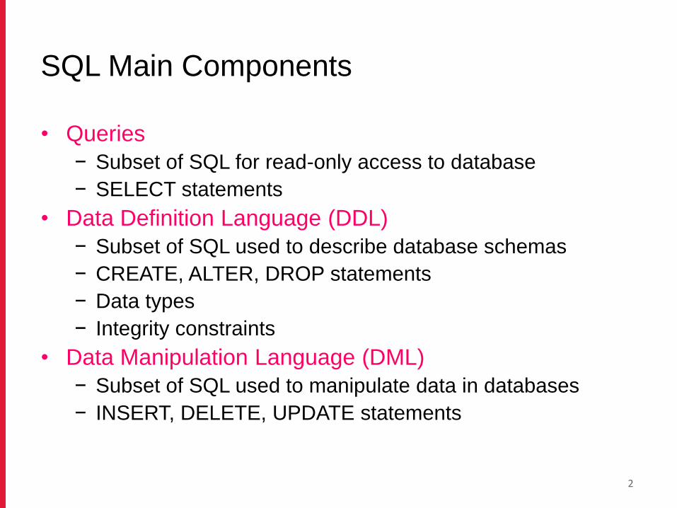
SQL Main Components

• Queries

− Subset of SQL for read-only access to database

− SELECT statements

• Data Definition Language (DDL)

− Subset of SQL used to describe database schemas

− CREATE, ALTER, DROP statements

− Data types

− Integrity constraints

• Data Manipulation Language (DML)

− Subset of SQL used to manipulate data in databases

− INSERT, DELETE, UPDATE statements

2

DATA DEFINITION LANGUAGE (DDL)

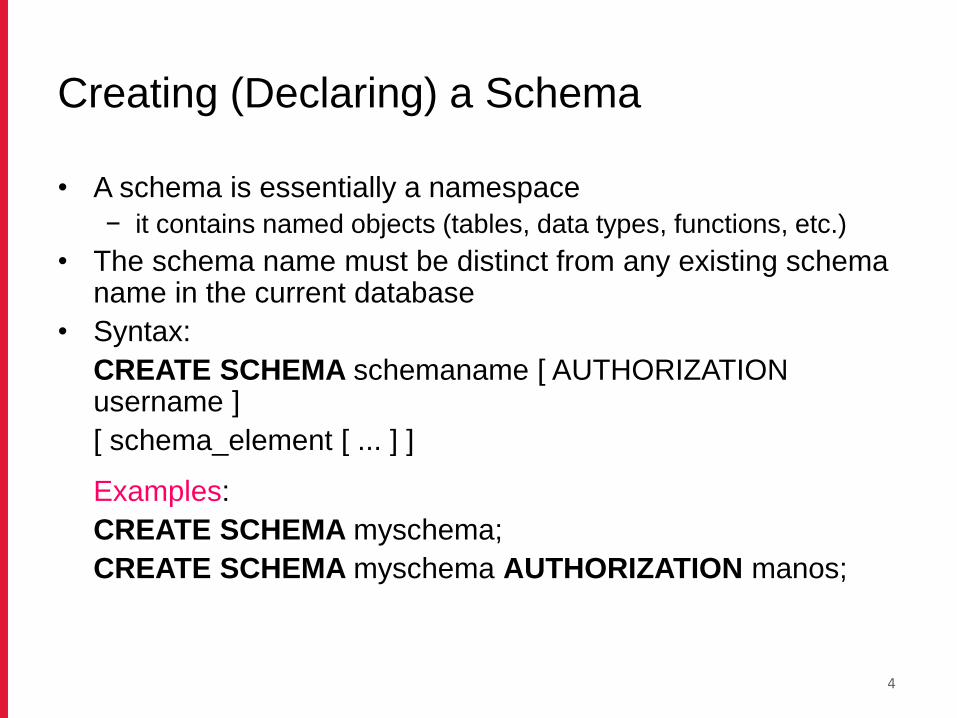
Creating (Declaring) a Schema

• A schema is essentially a namespace

− it contains named objects (tables, data types, functions, etc.)

• The schema name must be distinct from any existing schema name in the current database

• Syntax:

CREATE SCHEMA schemaname [ AUTHORIZATION username ]

[ schema_element [ ... ] ]

Examples:

CREATE SCHEMA myschema;

CREATE SCHEMA myschema AUTHORIZATION manos;

4

Creating (Declaring) a Relation/Table

• To create a relation:

CREATE TABLE <name> (

<list of elements>

);

• To delete a relation:

DROP TABLE <name>;

• To alter a relation (add/remove column):

ALTER TABLE <name> ADD <element>

ALTER TABLE <name> DROP <element>

5

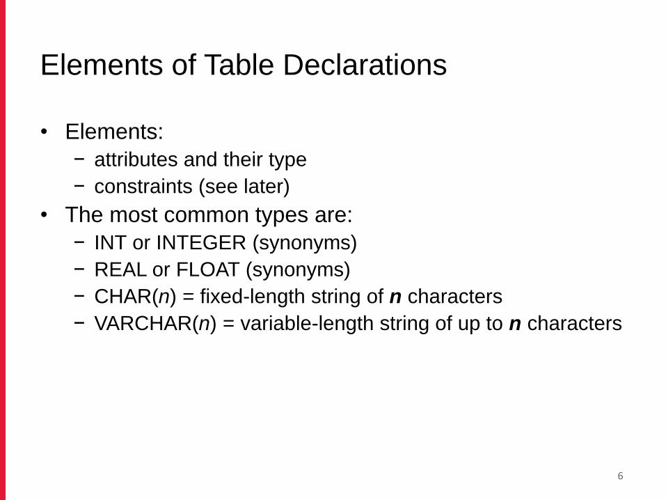
Elements of Table Declarations

• Elements:

− attributes and their type

− constraints (see later)

• The most common types are:

− INT or INTEGER (synonyms)

− REAL or FLOAT (synonyms)

− CHAR(n) = fixed-length string of n characters

− VARCHAR(n) = variable-length string of up to n characters

6

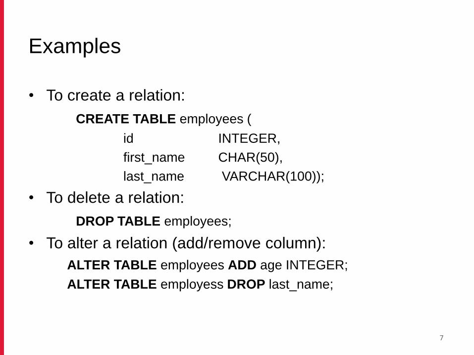
Examples

• To create a relation:

CREATE TABLE employees (

id INTEGER,

first_name CHAR(50),

last_name VARCHAR(100));

• To delete a relation:

DROP TABLE employees;

• To alter a relation (add/remove column):

ALTER TABLE employees ADD age INTEGER;

ALTER TABLE employess DROP last_name;

7

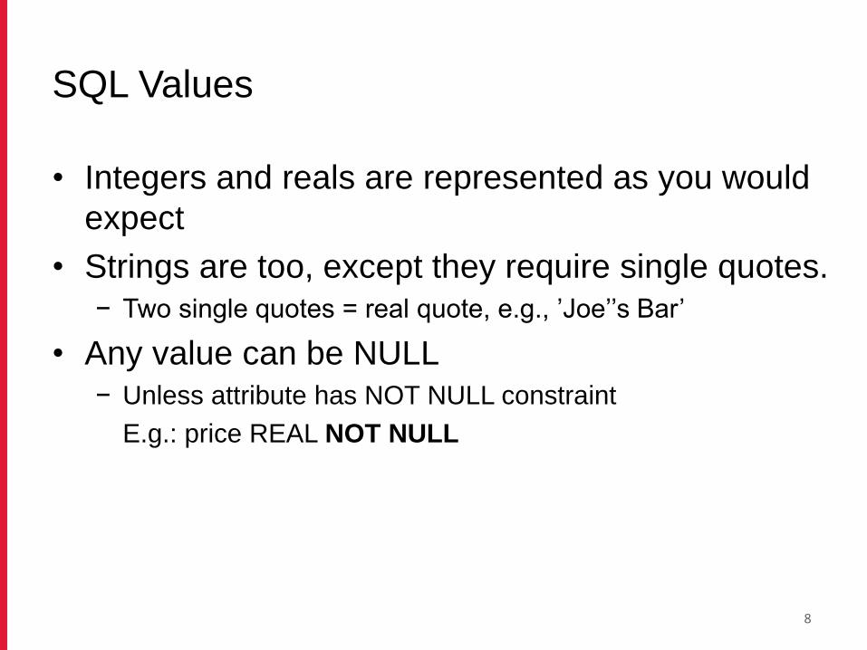
SQL Values

• Integers and reals are represented as you would

expect

• Strings are too, except they require single quotes.

− Two single quotes = real quote, e.g., ’Joe’’s Bar’

• Any value can be NULL

− Unless attribute has NOT NULL constraint

E.g.: price REAL NOT NULL

8

Dates and Times

• DATE and TIME are types in SQL.

− The form of a date value is: DATE ‘yyyy-mm-dd’

Example (for Oct. 19, 2011):

DATE ‘2011-10-19’

− The form of a time value is: TIME ‘hh:mm:ss’ with an optional decimal point and fractions of a second following.

Example (for two and a half seconds after 6:40PM):

TIME ‘18:40:02.5’

9

INTEGRITY CONSTRAINTS

10

Running Example

Beers(name, manf)

Bars(name, addr, license)

Drinkers(name, addr, phone)

Likes(drinker, beer)

Sells(bar, beer, price)

Frequents(drinker, bar)

Underline = key (tuples cannot have the same value in all key attributes)

− Excellent example of a constraint

11

Kinds of Constraints

• Keys

• Foreign-key or referential-integrity constraints

− Inter-relation constraints

• Value-based constraints

− Constrain values of a particular attribute

• Tuple-based constraints

− Relationship among components

• Assertions

12

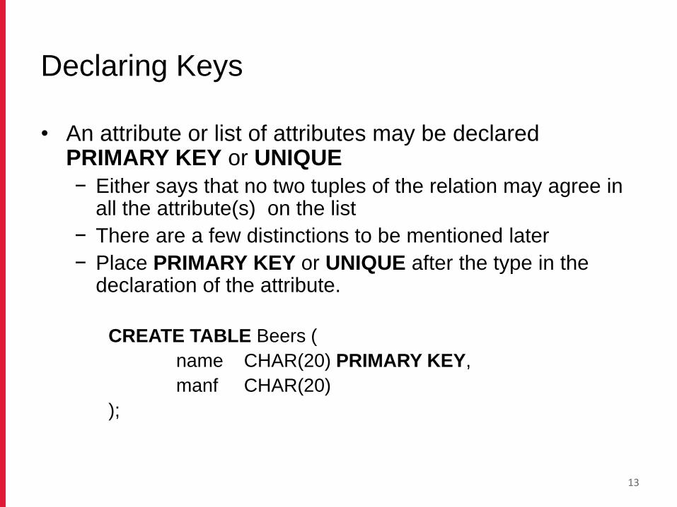
Declaring Keys

• An attribute or list of attributes may be declared PRIMARY KEY or UNIQUE

− Either says that no two tuples of the relation may agree in all the attribute(s) on the list

− There are a few distinctions to be mentioned later

− Place PRIMARY KEY or UNIQUE after the type in the declaration of the attribute.

CREATE TABLE Beers (

name CHAR(20) PRIMARY KEY,

manf CHAR(20)

);

13

Declaring Multi-attribute Keys

• A key declaration can appear as element in the list of elements of a CREATE TABLE statement

• This form is essential if the key consists of more than one attribute

CREATE TABLE Sells (

bar CHAR(20),

beer VARCHAR(20),

price REAL,

PRIMARY KEY (bar, beer));

The bar and beer together are the key for Sells

14

PRIMARY KEY vs. UNIQUE

• There can be only one PRIMARY KEY for a relation, but

several UNIQUE attributes

• No attribute of a PRIMARY KEY can ever be NULL in

any tuple. But attributes declared UNIQUE may have

NULL’s, and there may be several tuples with NULL.

15

Foreign Keys

• Values appearing in attributes of one relation must appear

together in certain attributes of another relation

Example:

We might expect that a value in Sells.beer also appears

as value in Beers.name

Beers(name, manf)


16

Expressing Foreign Keys

• Use keyword REFERENCES, either:

− After an attribute (for one-attribute keys)

REFERENCES <relation> (<attributes>)

− As an element of the schema:

FOREIGN KEY (<list of attributes>)

REFERENCES <relation> (<attributes>)

• Referenced attributes must be declared PRIMARY KEY

or UNIQUE

17

Example: With Attribute



manf CHAR(20) );


bar CHAR(20),

beer CHAR(20) REFERENCES Beers(name),

price REAL );

18

Example: As Schema Element



manf CHAR(20) );


bar CHAR(20),

beer CHAR(20),

price REAL,

FOREIGN KEY(beer) REFERENCES Beers(name));

19

Enforcing Foreign-Key Constraints

• If there is a foreign-key constraint from relation R to relation S,

two violations are possible:

− An insert or update to R introduces values not found in S

− A deletion or update to S causes some tuples of R to “dangle”

Example: suppose R = Sells, S = Beers

• An insert or update to Sells that introduces a non-existent beer

must be rejected

• A deletion or update to Beers that removes a beer value found

in some tuples of Sells can be handled in three ways (next

slide).

20

Actions Taken

• DEFAULT: Reject the modification

− Deleted beer in Beer: reject modifications in Sells tuples

− Updated beer in Beer: reject modifications in Sells tuples

• CASCADE: Make the same changes in Sells

− Deleted beer in Beer: delete Sells tuple

− Updated beer in Beer: change value in Sells

• SET NULL: Change the beer to NULL

− Deleted beer in Beer: set NULL values in Sells tuples

− Updated beer in Beer: set NULL values in Sells tuples

21

Example

• Delete the ‘Bud’ tuple from Beers− DEFAULT: do not change any tuple from Sells that have beer =

‘Bud’

− CASCADE: delete all tuples from Sells that have beer = ’Bud

− SET NULL: Change all tuples of Sells that have beer = ’Bud’ to have beer = NULL

• Update the ‘Bud’ tuple to ’Budweiser’− DEFAULT: do not change any tuple from Sells that have beer =

‘Bud’

− CASCADE: change all Sells tuples with beer = ’Bud’ to beer = ’Budweiser’

− SET NULL: Same change as for deletions

23

Choosing a Policy

• When we declare a foreign key, we may choose policies

SET NULL or CASCADE independently for deletions and

updates

• Follow the foreign-key declaration by:

ON [UPDATE, DELETE][SET NULL, CASCADE]

• Two such clauses may be used, otherwise, the default

(reject) is used.

24

Example: Setting a Policy


bar CHAR(20),

beer CHAR(20),

price REAL,

FOREIGN KEY(beer) REFERENCES Beers(name)

ON DELETE SET NULL

ON UPDATE CASCADE

);

25

Attribute-Based Checks

• Constraints on the value of a particular attribute

• Add CHECK(<condition>) to the declaration for the

attribute

• The condition may use the name of the attribute, but any

other relation or attribute name must be in a subquery

26

Example: Attribute-based Check


bar CHAR(20),

beer CHAR(20) CHECK (beer IN(

SELECT name FROM Beers)),

price REAL CHECK (price <= 5.00 )

);

27

Timing of Checks

• Attribute-based checks are performed only when a value

for that attribute is inserted or updated

• Example:

− CHECK (price <= 5.00)

Checks every new price and rejects the modification (for

that tuple) if the price is more than $5

− CHECK (beer IN (SELECT name FROM Beers))

Not checked if a beer is later deleted from Beers (unlike

foreign-keys)

28

Tuple-Based Checks

• CHECK (<condition>) may be added as a relation-schema element

− The condition may refer to any attribute of the relation, but other attributes or relations require a subquery

− Checked on insert or update only

Example: Only Joe’s Bar can sell beer for more than $5:


bar CHAR(20),

beer CHAR(20),

price REAL,

CHECK (bar = ’Joe’’s Bar’ OR price <= 5.00));

29

Assertions

• Permit the definition of constraints over whole tables, rather

than individual tuples

− useful in many situations -- e.g., to express generic inter-relational

constraints

− An assertion associates a name to a check clause. Syntax:

CREATE ASSERTION AssertName CHECK (Condition)

Example:

"There must always be at least one tuple in table Employee":

CREATE ASSERTION AlwaysOneEmployee

CHECK (1 <= (SELECT count(*) FROM Employee))

30

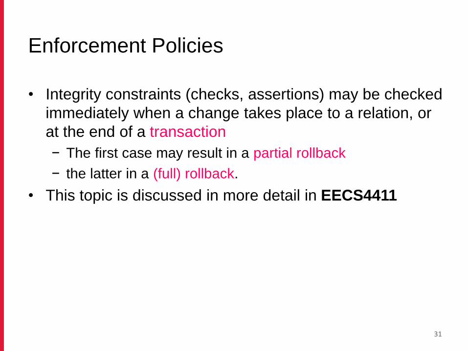
Enforcement Policies

• Integrity constraints (checks, assertions) may be checked

immediately when a change takes place to a relation, or

at the end of a transaction

− The first case may result in a partial rollback

− the latter in a (full) rollback.

• This topic is discussed in more detail in EECS4411

31

DATA MANIPULATION LANGUAGE (DML)

Data Manipulation Language (DML)

• Syntax elements used for inserting, deleting and updating

data in a database

• Modification statements include:

− INSERT - for inserting data in a database

− DELETE - for deleting data in a database

− UPDATE - for updating data in a database

• All modification statements operate on a set of tuples (no

duplicates)

33

Example

Employee(FirstName,Surname,Dept,Office,Salary,City)

Department(DeptName, Address, City)

Product(Code,Name,Description,ProdArea)

LondonProduct(Code,Name,Description)

34

Insertions

Syntax varies:

• Using only values:

INSERT INTO Department

VALUES (‘Production’, ‘Rue du Louvre 23’, ’Toulouse’)

• Using both column names and values:

INSERT INTO Department(DeptName, City)

VALUES (‘Production’, ’Toulouse’)

• Using a subquery:

INSERT INTO LondonProducts

(SELECT Code, Name, Description

FROM Product

WHERE ProdArea = ‘London’)

35

Notes on Insertions

• The ordering of attributes (if present) and of

values is meaningful -- first value for the first

attribute, etc.

• If AttributeList is omitted, all the relation attributes

are considered, in the order they appear in the

table definition

• If AttributeList does not contain all the relation

attributes, left-out attributes are assigned default

values (if defined) or the NULL value

36

Deletions

Syntax:

DELETE FROM TableName [WHERE Condition]

• "Remove the Production department":

DELETE FROM Department

WHERE DeptName = ‘Production’

• "Remove departments with no employees":


WHERE DeptName NOT IN (SELECT Dept FROM Employee)

37

Notes on Deletions

• The DELETE statement removes from a table all tuples

that satisfy a condition

• If the WHERE clause is omitted, DELETE removes all

tuples from the table (keeps the table schema):


• The removal may produce deletions from other tables –

(see referential integrity constraint with cascade policy)

• To remove table Department completely (content and

schema) :

DROP TABLE Department CASCADE

38

Updates

Syntax:

UPDATE TableNameSET Attribute = < Expression | SelectSQL | null | default >{, Attribute = < Expression | SelectSQL | null | default >}[ WHERE Condition ]

• Examples:

UPDATE Employee

SET Salary = Salary + 5

WHERE RegNo = ‘M2047’

UPDATE Employee

SET Salary = Salary * 1.1

WHERE Dept = ‘Administration’

39

Notes on Updates

• The order of updates is important:

UPDATE Employee


WHERE Salary <= 30

UPDATE Employee


WHERE Salary > 30

• In this example, some employees may get a double raise

(e.g., employee with salary 29)! How can we fix this?

40

Views

• A view is a relation defined in terms of stored tables

(called base tables) and other views.

• Two kinds:

− Virtual = not stored in the database; just a query for

constructing the relation

CREATE VIEW <name> AS <query>;

− Materialized = actually constructed and stored

CREATE MATERIALIZED VIEW <name> AS

<query>;

42

Running Example

Beers(name, manf)

Bars(name, addr, license)

Drinkers(name, addr, phone)

Likes(drinker, beer)


Frequents(drinker, bar)

43

Example: View Definition

CanDrink(drinker, beer) is a view “containing” the drinker-

beer pairs such that the drinker frequents at least one bar

that serves the beer:

CREATE VIEW CanDrink AS

SELECT drinker, beer

FROM Frequents, Sells

WHERE Frequents.bar = Sells.bar;

44

Example: Accessing a View

Query a view as if it were a base table:

SELECT beer

FROM CanDrink

WHERE drinker = ’Sally’;

45

Notes on Views

• Data independence (hide schema from apps)

− DB team splits CustomerInfo into Customer and Address

− View accomodates changes with web apps

• Data hiding (access data on need-to-know basis)

− Doctor outsources patient billing to third party

− View restricts access to billing-related patient info

• Code reuse

− Very similar subquery appears multiple times in a query

− View shortens code, improves readability, reduces bugs, …

− Bonus: query optimizer often does a better job!

46

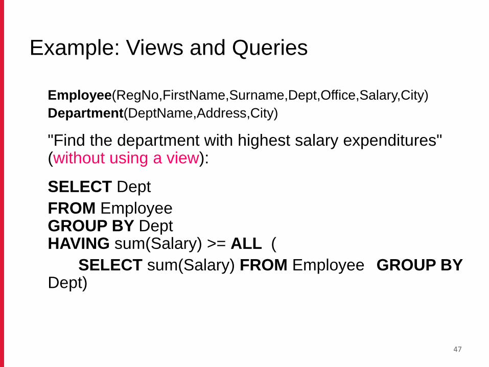
Example: Views and Queries

Employee(RegNo,FirstName,Surname,Dept,Office,Salary,City)

Department(DeptName,Address,City)

"Find the department with highest salary expenditures" (without using a view):

SELECT Dept

FROM EmployeeGROUP BY DeptHAVING sum(Salary) >= ALL (

SELECT sum(Salary) FROM Employee GROUP BY Dept)

47

Example: Views and Queries (cont.)

"Find the department with highest salary expenditures" (using a view):

CREATE VIEW SalBudget (Dept, SalTotal) ASSELECT Dept, sum(Salary)

FROM Employee

GROUP BY Dept

SELECT Dept

FROM SalBudget

WHERE SalTotal = (SELECT max(SalTotal) FROM SalBudget)

48

Updates on Views

• Generally, it is impossible to modify a virtual view because

it doesn’t exist

• Can’t we “translate” updates on views into “equivalent”

updates on base tables?

− Not always (in fact, not often)

− Most systems prohibit most view updates

49

Example:The View

CREATE VIEW Synergy AS

SELECT Likes.drinker, Likes.beer, Sells.bar

FROM Likes, Sells, Frequents

WHERE Likes.drinker = Frequents.drinker

AND Likes.beer = Sells.beer

AND Sells.bar = Frequents.bar;

50

Pick one copy ofeach attribute

Join of Likes, Sells, and Frequents

Interpreting a View Insertion

• We cannot insert into Synergy - it is a virtual view

• Idea: Try to translate a (drinker, beer, bar) triple into three insertions of projected pairs, one for each of Likes, Sells, and Frequents.

− Sells.price will have to be NULL.

− There isn’t always a unique translation

51

Need for SQL Triggers - Not discussed

Materialized Views

• Problem: each time a base table changes, the

materialized view may change

− Cannot afford to recompute the view with each change

• Solution: Periodic reconstruction of the materialized view,

which is otherwise “out of date”

52

Example: A Data Warehouse

• Wal-Mart stores every sale at every store in a database

• Overnight, the sales for the day are used to update a data

warehouse = materialized views of the sales

• The warehouse is used by analysts to predict trends and

move goods to where they are selling best

53

INDEXES (INDICES)

54

Index

• Problem: needle in haystack

− Find all phone numbers with first name ‘Mary’

− Find all phone numbers with last name ‘Li’

• Index: auxiliary database structure which provides random

access to data

− Index a set of attributes. No standard syntax! Typical is:

CREATE INDEX indexName ON TableName(AttributeList);

− Random access to any indexed attribute

(e.g., retrieve a single tuple out of billions in <5 disk accesses)

− Similar to a hash table, but in a DBMS it is a balanced search

tree with giant nodes (a full disk page) called a B-tree

55

Example: Using Index

SELECT fname

FROM people

WHERE lname = ‘Papagelis‘

• Without an index:

The DBMS must look at the lname column on every row in the table (this is known as a full table scan)

• With an index (defined on attribute lname):

The DBMS simply follows the B-tree data structure until the ‘Papagelis’ entry has been found

This is much less computationally expensive than a full table scan

56

Another Example: Using Index

CREATE INDEX BeerInd ON Beers(manf);

CREATE INDEX SellInd ON Sells(bar, beer);

Query: Find the prices of beers manufactured by Pete’s and sold by Joe’s bar

SELECT price FROM Beers, Sells

WHERE manf = ’Pete’’s’ AND Beers.name = Sells.beer

AND bar = ’Joe’’s Bar’;

DBMS uses:

• BeerInd to get all the beers made by Pete’s fast

• SellInd to get prices of those beers, with bar = ’Joe’’s Bar’ fast

57

Database Tuning

• How to make a database run fast?

− Decide which indexes to create

• Pro: An index speeds up queries that can use it

• Con: An index slows down all modifications on its relation

as the index must be modified too

58

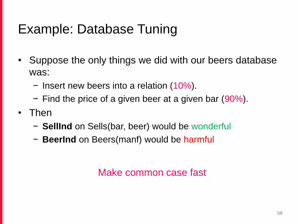
Example: Database Tuning

• Suppose the only things we did with our beers database

was:

− Insert new beers into a relation (10%).

− Find the price of a given beer at a given bar (90%).

• Then

− SellInd on Sells(bar, beer) would be wonderful

− BeerInd on Beers(manf) would be harmful

Make common case fast

59

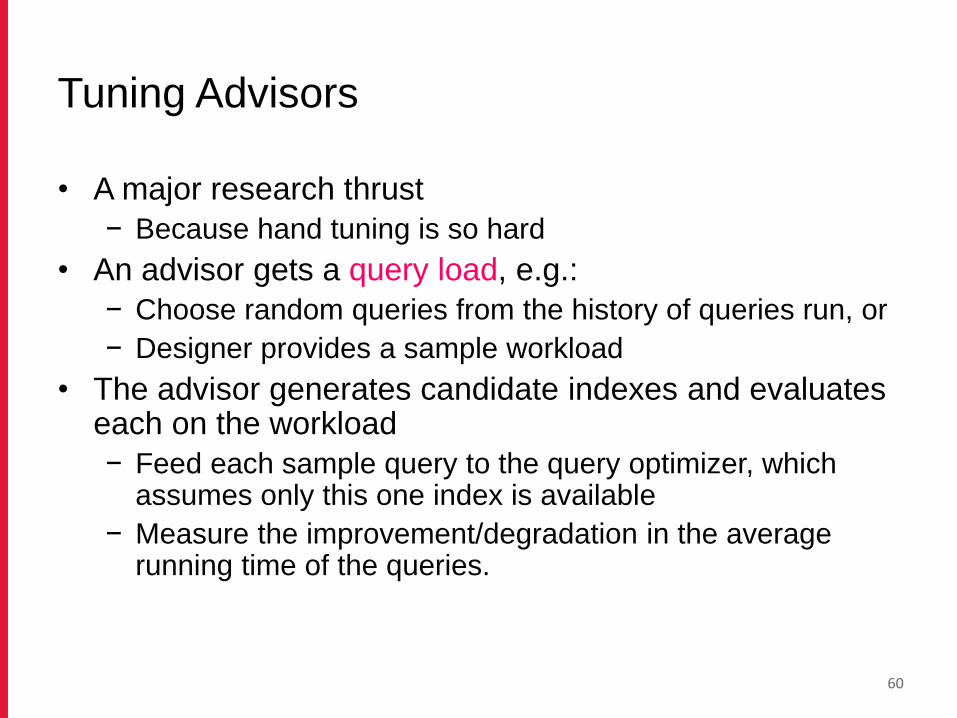
Tuning Advisors

• A major research thrust

− Because hand tuning is so hard

• An advisor gets a query load, e.g.:

− Choose random queries from the history of queries run, or

− Designer provides a sample workload

• The advisor generates candidate indexes and evaluates each on the workload

− Feed each sample query to the query optimizer, which assumes only this one index is available

− Measure the improvement/degradation in the average running time of the queries.

60

What’s Next?

• Embedded SQL

− Part of Assignment 2

• DB Security (moved to last lecture, if time)

− SQL Injection Issues

61

data manipulation language (dml) data definition language ...€¦ · enforcing foreign-key...

Documents