data-driven multi-stage scenario tree generation via...

Data-Driven Multi-Stage Scenario Tree Generation viaStatistical Property and Distribution Matching

Bruno A. Calfa∗, Anshul Agarwal†, Ignacio E. Grossmann∗, John M. Wassick†

October 24, 2013

Abstract

The objective of this paper is to bring systematic methods for scenario tree generationto the attention of the Process Systems Engineering community. In this paper, we fo-cus on a general, data-driven optimization-based method for generating scenario trees,which does not require strict assumptions on the probability distributions of the un-certain parameters. This method is based on the Moment Matching Problem (MMP),originally proposed by Høyland & Wallace (2001). In addition to matching moments,and in order to cope with potentially under-specified MMP, we propose matching (Em-pirical) Cumulative Distribution Function information of the uncertain parameters.The new method gives rise to a Distribution Matching Problem (DMP) that is aidedby predictive analytics. We present two approaches for generating multi-stage scenariotrees by considering time series modeling and forecasting. The aforementioned tech-niques are illustrated with a motivating production planning problem with uncertaintyin production yield and correlated product demands.

Keywords: Process Systems Engineering, Stochastic Programming, Scenario Genera-tion, Distribution Matching Problem, Time Series Forecasting, Analytics

1 IntroductionThe importance of accounting for uncertainty in mathematical optimization was recognizedin its early days in the seminal and influential paper by George B. Dantzig (Dantzig, 1955).Two of the current popular optimization frameworks that incorporate uncertainty in the mod-eling stage are Robust Optimization (Ben-Tal, Ghaoui, & Nemirovski, 2009) and StochasticProgramming (Birge & Louveaux, 2011). In this paper, we focus on Stochastic Programming(SP) and address the issue of scenario generation.

To illustrate the many possible sources of uncertainty in Process Systems Engineering(PSE), consider as an example a production planning problem for a network of chemicalplants. Planning decisions usually span multiple time periods and generally involve, but are∗Department of Chemical Engineering. Carnegie Mellon University. Pittsburgh, PA, 15213, USA.†The Dow Chemical Company. Midland, MI, 48674, USA.

1

1 Introduction

not limited to determining the amount of raw materials to be purchased by each plant, theproduction and inventory levels at each plant, the transportation of intermediate and finishedproducts between different locations, and meeting the forecast demand. It is clear that allthose decisions may be subject to some kind of uncertainty. For instance, the availabilityof a key raw material may be uncertain, i.e. there may be shortage for certain months ina year. Another example is the possibility of mechanical failure of pieces of equipment ina plant or its complete unplanned shutdown, which affects the entire network. Two typesof uncertainty are reported in the literature (Goel & Grossmann, 2006): exogenous (e.g.,market) and endogenous (e.g., decision-dependent). A review on optimization methods withexogenous uncertainties can be found in Sahinidis (2004).

A central aspect of Stochastic Programming is the definition of scenarios, which describepossible values that the uncertain parameters or stochastic processes may take. Applicationsin PSE that make explicit use of scenarios expand multiple areas and time scales. Some repre-sentative examples are: dynamic optimization (Abel & Marquardt, 2000), scheduling (Guil-lén, Espuña, & Puigjaner, 2006; Colvin & Maravelias, 2009; Pinto-Varela, Barbosa-Povoa, &Novais, 2009), planning (Sundaramoorthy, Evans, & Barton, 2012; Li & Ierapetritou, 2011;You, Wassick, & Grossmann, 2009; Gupta & Grossmann, 2012), and synthesis and design(Kim, Realff, & Lee, 2011; Chen, Adams II, & Barton, 2011). The most common assumptionmade in the works listed before is that the scenario tree is given (probabilities and values ofuncertain parameters at every node are known). That is, the “true” probability distributionsare known, and the uncertainty typically is characterized by arbitrary deviations from someaverage value based on minimum and maximum values (for instance: low, medium, and highvalues with probabilities arbitrarily chosen).

Researchers have also developed decomposition algorithms to tackle large-scale and real-world instances that originate from explicitly considering scenarios in optimization problems.We argue that it is equally important to generate scenario trees that satisfactorily capturethe uncertainty in a given problem, as the quality of the solution to the SP problem is directlyinfluenced by the accuracy of the scenarios. Therefore, it is important to apply systematicscenario generation methods instead of making assumptions that may be questionable. King& Wallace (2012) wrote an excellent book on the challenges of optimization modeling underuncertainty. The authors also discuss the importance of generating meaningful scenarios(see Chapter 4), as modeling with SP results in a framework with practical and robustdecision-making capability.

These data-driven approaches to optimization problems have become common in theOperations Research and Management Science communities, and are an example of what iscalled Business Analytics (BA) (Bartlett, 2013). After the data collection and managementphase, BA leverages data analysis to make analytics-based decisions that can be divided intothree general layers: descriptive (querying and reporting, databases), predictive (forecastingand simulation), and prescriptive (deterministic and stochastic optimization) (Davenport &Harris, 2007). The data-driven scenario generation method described in this paper can belinked with the descriptive and predictive layers, and then used for decision-making in theprescriptive layer.

It is worth noting that, even though not usually regarded as a scenario generation method,the Sample Average Approximation (SAA) method (Kleywegt, Shapiro, & Homem-de-Mello,2001; Shapiro, 2006) can be used to approximate the continuous probability distribution

October 24, 2013 2 of 38

2 Two-Stage Scenario Tree Generation

assumed for the uncertain parameters. Specifically, the distributions are sampled, for in-stance via Monte Carlo sampling, and the expected value function is approximated by thecorresponding sample average function, which is repeatedly solved until some convergencecriterion is met. The size of the sample must be such that a degree of confidence on the finalobjective function value is satisfied. In addition, the sampling step becomes more compli-cated in Multi-Stage SP (MSSP), as conditional sampling is required for the SAA methodto produce consistent estimators. Conditioning on previous events also plays a key role inthe moment matching method as discussed later in the paper.

The goal of this paper is to bring systematic methods for scenario tree generation tothe attention of the Process Systems Engineering community, and give an organizationalstructure to the formulations proposed in the literature thus far. We describe in detail themoment matching method for scenario tree generation. Different formulations of the MMPare presented. The main inputs or parameters to the MMP are the statistical moments ofeither time-independent random variables or stochastic processes. For the latter, statisti-cal properties can be obtained through the aid of time series forecasting models as will bedemonstrated. In order to cope with under-specified MMPs, we propose an extension tothe MMP, called Distribution Matching Problem (DMP), in which cumulative distributiondata are also matched. For completeness, we briefly present the ideas of scenario reduction(Dupačová, Gröwe-Kuska, & Römisch, 2003) and remark that moment matching and sce-nario reduction methods are not mutually exclusive. That is, a (dense) scenario tree canbe generated by matching statistical properties of the historical data, and then it can besystematically reduced so that the SP becomes tractable.

This paper is organized as follows. Section 2 introduces the moment matching methodas a systematic method to generate scenario trees. Enhancements to each formulation of theMoment Matching Problem are also proposed. The method is illustrated via a motivatingnumerical example for the optimal production planning of a network of chemical plants.Moreover, approaches for reducing the scenario tree are briefly discussed. Section 3 extendsthe methodology to the multi-stage case; the role of modeling stochastic processes is empha-sized and two approaches are described based on NLP and LP statistical property matchingformulations for generating multi-stage scenario trees. The approaches are illustrated witha numerical example, and conclusions are drawn in Section 4.

2 Two-Stage Scenario Tree GenerationIt is important to recall the role of scenario trees in Stochastic Programming (SP). Scenariotrees are an approximate discretized representation of the uncertainty in the data (Kaut,2003). They are based on discretized probability distributions to model the stochastic pro-cesses. The scenario trees are approximate because they contain a restricted number ofoutcomes in order to avoid the integration of continuous distribution functions. However,the size of the scenario trees directly impacts the computational complexity of SP models.

The concerns raised in the above paragraph have motivated the search for methodologiesthat can be used to systematically generate scenario trees. Two main classes of methodscan be identified: scenario generation and scenario reduction. In this section, we focus onscenario generation methods, in particular, the moment matching method, which was

October 24, 2013 3 of 38

2.1 L2 Moment Matching Problem 2 Two-Stage Scenario Tree Generation

originally proposed by Høyland & Wallace (2001) and is described as follows. Given aninitial structure of the tree, i.e. number of nodes per stage, it determines at each node thevalues for the random variables and their probabilities by solving a nonlinear programming(NLP) problem. The NLP problem minimizes the weighted squared error between statisticalproperties calculated from the outcomes or nodes, and the same properties calculated directlyfrom the data. Thus, it is based on an L2-norm formulation. If the absolute deviationsfrom the target properties are minimized as proposed by Ji et al. (2005), then an L1-normformulation can be employed, which has the advantage that it can be cast as an LP problem.In this paper, we present a new formulation of the MMP based on the L∞-norm. Examplesof statistical properties are the first four moments (expected value, variance, skewness, andkurtosis), covariance or correlation matrix, quantiles, etc.

In this section, we focus on two-stage problems in which the sources of uncertainty do nothave a time-series effect. In Section 3, we present approaches to generating scenario treeswith multiple stages where stochastic processes are the source of uncertainty.

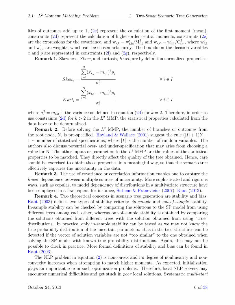
2.1 L2 Moment Matching ProblemIn the Moment Matching Problem (MMP), the uncertain parameters of the SP model be-come variables in a nonlinear optimization formulation as well as the probabilities of theoutcomes. The purpose of the MMP is to find the optimal values for the random variablesand probabilities (see Figure 1) of a pre-specified structure for the scenario tree that minimizethe error between the statistical properties calculated from the tree and the ones calculateddirectly from the data.

x1

p1

x2

p2

. . .xj

pj

. . .xN−1

pN−1

xN

pN

Figure 1: Two-stage scenario tree for one uncertain parameter.

In the L2 formulation, the squared error is employed in the objective function. Hence,the NLP formulation can be generically written as follows:

minx, p

∑s∈S

ws · (fs(x, p)− Svals)2

s.t.N∑j=1

pj = 1(1)

where x is a vector of random variables (uncertain parameters of the SP model), p is avector of probabilities of outcomes, s ∈ S is a statistical property to be matched (target), ws

is the weight for statistical property s, fs(·, ·) is the mathematical expression of statisticalproperty s calculated from the tree, Svals is the value of statistical property s (target value)

October 24, 2013 4 of 38


that characterizes the distribution of the data. Therefore, generating scenario trees via thesolution of the MMP is a data-driven approach in the sense that it does not require assumingspecific parametric probability distributions to model the uncertainty.

Any statistical property that somehow describes the data can be used to measure howwell the scenario tree represents them. Descriptive statistics provides measures that can beused to summarize and inform us about the probability distribution of the data. Four ofthese measures, called moments, (Papoulis, 1991), are the following: mean or expectation,and the central moments variance, skewness, and kurtosis. The mean or expectation tellsus about the average value in a data set, the variance is a measure of the spread of the dataabout the mean, the skewness is a measure of the asymmetry of the data, and the kurtosisis a measure of the thickness of the tails of the shape of the distribution of the data.

A more detailed definition of the L2 MMP is as follows. The uncertain data are indexedby i ∈ I, which denotes the entity of an uncertain parameter (for example, a product).N denotes the number of outcomes per node at the second stage, j ∈ J = {1, 2, . . . , N}denotes the branches (outcomes) from the root node, and k ∈ K = {1, 2, 3, 4} is the index ofthe first four moments. The decision variables are the uncertain parameters of the stochasticprogramming problem, xi,j, with corresponding probabilities of outcomes, pj. The momentscalculated from the tree are denoted by variables mi,k and the ones calculated from the dataare denoted by parameters Mi,k. Finally, the second co-moment, i.e. covariance, calculatedbetween entity i and i′ from the tree and the data are denoted by ci,i′ and Ci,i′ , respectively.The L2 MMP formulation is given as follows (see Gülpınar, Rustem, & Settergren (2004)).The goal is to generate a tree (determine the values of xi,j and pj) whose properties matchthose calculated from the data (Mi,k and, if applicable, Ci,i′).

(L2 MMP)

minx, p

zL2

MMP =∑i∈I

∑k∈K

wi,k(mi,k −Mi,k)2 +∑

(i, i′)∈Ii<i′

wi,i′(ci,i′ − Ci,i′)2 (2a)

s.t.N∑j=1

pj = 1 (2b)

mi,1 =N∑j=1

xi,jpj ∀ i ∈ I (2c)

mi,k =N∑j=1

(xi,j −mi,1)kpj ∀ i ∈ I, k > 1 (2d)

ci,i′ =N∑j=1

(xi,j −mi,1)(xi′,j −mi′,1)pj ∀ (i, i′) ∈ I, i < i′ (2e)

xi,j ∈ [xLBi,j , xUBi,j ] ∀ i ∈ I, j = 1, . . . , N (2f)pj ∈ [0, 1] ∀ j = 1, . . . , N (2g)

where the weighted squared error between the statistical properties calculated from the treeand inferred from the data is minimized in (2a), constraints (2b) ensure that the probabil-

October 24, 2013 5 of 38


ities of outcomes add up to 1, (2c) represent the calculation of the first moment (mean),constraints (2d) represent the calculation of higher-order central moments, constraints (2e)are the expressions for the covariance, and wi,k = w′i,k/M2

i,k and wi,i′ = w′i,i′/C2i,i′ , where w′i,k

and w′i,i′ are weights, which can be chosen arbitrarily. The bounds on the decision variablesx and p are represented in constraints (2f) and (2g), respectively.

Remark 1. Skewness, Skew, and kurtosis,Kurt, are by definition normalized properties:

Skewi =

N∑j=1

(xi,j −mi,1)3pj

σ3i

∀ i ∈ I

Kurti =

N∑j=1

(xi,j −mi,1)4pj

σ4i

∀ i ∈ I

where σ2i = mi,2 is the variance as defined in equation (2d) for k = 2. Therefore, in order to

use constraints (2d) for k > 2 in the L2 MMP, the statistical properties calculated from thedata have to be denormalized.

Remark 2. Before solving the L2 MMP, the number of branches or outcomes fromthe root node, N, is pre-specified. Høyland & Wallace (2001) suggest the rule (|I| + 1)N −1 ∼ number of statistical specifications, where |I| is the number of random variables. Theauthors also discuss potential over- and under-specification that may arise from choosing avalue for N. The other inputs or parameters to the L2 MMP are the values of the statisticalproperties to be matched. They directly affect the quality of the tree obtained. Hence, careshould be exercised to obtain those properties in a meaningful way, so that the scenario treeeffectively captures the uncertainty in the data.

Remark 3. The use of covariance or correlation information enables one to capture thelinear dependence between multiple sources of uncertainty. More sophisticated and rigorousways, such as copulas, to model dependency of distributions in a multivariate structure havebeen employed in a few papers, for instance, Sutiene & Pranevicius (2007); Kaut (2013).

Remark 4. Two theoretical concepts in scenario tree generation are stability and bias.Kaut (2003) defines two types of stability criteria: in-sample and out-of-sample stability.In-sample stability can be checked by comparing the solutions to the SP model from usingdifferent trees among each other, whereas out-of-sample stability is obtained by comparingthe solutions obtained from different trees with the solution obtained from using “true”distributions. In practice, only in-sample stability can be tested as we may not know thetrue probability distribution of the uncertain parameters. Bias in the tree structures can bedetected if the vector of solution variables are not “too similar” to the one obtained whensolving the SP model with known true probability distributions. Again, this may not bepossible to check in practice. More formal definitions of stability and bias can be found inKaut (2003).

The NLP problem in equation (2) is nonconvex and its degree of nonlinearity and non-convexity increases when attempting to match higher moments. As expected, initializationplays an important role in such optimization problems. Therefore, local NLP solvers mayencounter numerical difficulties and get stuck in poor local solutions. Systematic multi-start

October 24, 2013 6 of 38

2.2 L1 and L∞ Moment Matching Problems 2 Two-Stage Scenario Tree Generation

methods can be used with local NLP solvers to help overcome the problems aforementionedby sampling multiple starting points in the feasible region and solving the NLP problemusing each different starting point; however, it must be recognized that multi-start methodsare not a panacea and there is no guarantee of systematically obtaining a global (or nearglobal) solution to the MMP. Finally, deterministic global optimization solvers can also beused although at considerable computational expense.

2.2 L1 and L∞ Moment Matching ProblemsIf the absolute value of the deviations from the target moments and co-moments are min-imized, then the MMP becomes an L1-norm model as proposed by Ji et al. (2005). Awell-known reformulation of the nondifferentiable absolute value function in the definition ofthe objective function consists in splitting the variable in its argument into two non-negativevariables, which correspond to the positive and negative values of the original variable.

The L1 formulation of the MMP is then as follows. Partition the moment and covariancevariables, mi,k and ci,i′ , respectively, into their positive and negative parts m+

i,k, m−i,k, c+i,i′ ,

and c−i,i′ . Thus, the L1 MMP is given by:

(L1 MMP)

minx, p

zL1

MMP =∑i∈I

∑k∈K

wi,k(m+i,k +m−i,k) +

∑(i, i′)∈Ii<i′

wi,i′(c+i,i′ + c−i,i′) (3a)

s.t.N∑j=1

pj = 1 (3b)

N∑j=1

xi,jpj +m+i,1 −m−i,1 = Mi,1 ∀ i ∈ I (3c)

N∑j=1

(xi,j −N∑j′=1

xi,j′pj′)kpj +m+i,k −m−i,k = Mi,k ∀ i ∈ I, k > 1 (3d)

N∑j=1

(xi,j −N∑j′=1

xi,j′pj′)(xi′,j −N∑j′=1

xi′,j′pj′)pj + c+i,i′ − c−i,i′ = Ci,i′ ∀ (i, i′) ∈ I, i < i′

(3e)m+i,k, m

−i,k ≥ 0 ∀ i ∈ I, k ∈ K (3f)

c+i,i′ , c

−i,i′ ≥ 0 ∀ (i, i′) ∈ I, i < i′

(3g)xi,j ∈ [xLBi,j , xUBi,j ] ∀ i ∈ I, j = 1, . . . , N

(3h)pj ∈ [0, 1] ∀ j = 1, . . . , N (3i)

where the weighted absolute deviations between the statistical properties calculated fromthe tree and inferred from the data are minimized in (3a), constraints (3b) ensure that the

October 24, 2013 7 of 38

2.2 L1 and L∞ Moment Matching Problems 2 Two-Stage Scenario Tree Generation

probabilities of outcomes add up to 1, (3c) attempts to match the first moment (mean),constraints (3d) represent the matching of higher-order central moments, constraints (3e)attempt to match the covariance, and wi,k = |w′i,k/Mi,k| and wi,i′ = |w′i,i′/Ci,i′|, where w′i,kand w′i,i′ are weights that can be arbitrarily chosen. The bounds on the variables x, p, m+,m−, c+, and c− are represented by constraints (3f) – (3i).

Another way of formulating the MMP is through the minimization of the L∞-norm ofthe deviations with respect to the targets.

(L∞ MMP)

minx, p

zL∞

MMP = µ+ γ (4a)

s.t.

Constraints (3b) – (3i)µ ≥ wi,km

+i,k ∀ i ∈ I, k ∈ K (4b)

µ ≥ wi,km−i,k ∀ i ∈ I, k ∈ K (4c)

γ ≥ wi,i′c+i,i′ ∀ (i, i′) ∈ I, i < i′ (4d)

γ ≥ wi,i′c−i,i′ ∀ (i, i′) ∈ I, i < i′ (4e)

where µ and γ are scalar variables that account for the maximum deviations in the momentsand covariances, respectively.

2.2.1 Linear Programming L1 and L∞ MMPs

The L2, L1, and L∞ MMPs shown in equations (2), (3), and (4), respectively, are nonlinearand nonconvex due to the mathematical expressions for the moments since both probabil-ities and node values are decision variables. Ji et al. (2005) used ideas from Linear GoalProgramming and proposed an LP formulation for the L1 MMP in which only probabili-ties are decision variables. In this LP formulation, the node values are generally obtainedvia some simulation approach. For time-dependent data, such as asset returns in financialportfolio management applications, a time-series model is used to forecast future expectedvalues and possibly higher moments. Multiple values above and below the forecast expectedvalue can be used as the node values or outcomes in the L1 and L∞ LP MMP formulationsand the probabilities of each outcome are left as the decision variables. In PSE applications,uncertain parameters that typically have a time component are product demand and marketprice.

Let xi,j be a parameter with the value of the uncertain parameter that can be arbitrarilychosen or calculated from some simulation procedure, for example simulation of time-seriesforecasting models. As long as there are at least two values, for example xi,j and xi,j′ , thatare symmetric with respect to the mean, then the expected value can always be matched(see Proposition 1 in Ji et al. (2005)) and the L1 LP MMP is given as follows:

October 24, 2013 8 of 38

2.3 Remarks on the MMP Formulations 2 Two-Stage Scenario Tree Generation

(L1 LP MMP)

minp

zL1

LP MMP =∑i∈I

∑k∈K\{1}

wi,k(m+i,k +m−i,k) +

∑(i, i′)∈Ii<i′

wi,i′(c+i,i′ + c−i,i′) (5a)

s.t.N∑j=1

pj = 1 (5b)

N∑j=1

xi,jpj = Mi,1 ∀ i ∈ I (5c)

N∑j=1

(xi,j −Mi,1)kpj +m+i,k −m−i,k = Mi,k ∀ i ∈ I, k > 1 (5d)

N∑j=1

(xi,j −Mi,1)(xi′,j −Mi′,1)pj + c+i,i′ − c−i,i′ = Ci,i′ ∀ (i, i′) ∈ I, i < i′ (5e)

m+i,k, m

−i,k ≥ 0 ∀ i ∈ I, k ∈ K (5f)

c+i,i′ , c

−i,i′ ≥ 0 ∀ (i, i′) ∈ I, i < i′ (5g)

pj ∈ [0, 1] ∀ j = 1, . . . , N (5h)

Likewise, the L∞ LP MMP can be formulated as follows:

(L∞ LP MMP)

minp

zL∞

LP MMP = µ+ γ (6a)

s.t.

Constraints (5b) – (5h)µ ≥ wi,km

+i,k ∀ i ∈ I, k ∈ K (6b)

µ ≥ wi,km−i,k ∀ i ∈ I, k ∈ K (6c)

γ ≥ wi,i′c+i,i′ ∀ (i, i′) ∈ I, i < i′ (6d)

γ ≥ wi,i′c−i,i′ ∀ (i, i′) ∈ I, i < i′ (6e)

Obviously, it may be more advantageous to solve an LP problem instead of a nonconvexNLP problem. For multi-stage stochastic problems with time-dependent uncertain parame-ters, the solution strategy is much more complex when applying the NLP model instead ofthe LP formulation. Details are given in Sections 3.1 and 3.2.

2.3 Remarks on the MMP FormulationsEach Lp-norm formulation for the MMP produces different solutions, i.e. different valuesof probabilities, and when applicable, outcomes. This can be explained by the properties ofLp-norms of vectors. To illustrate, consider a vector x ∈ R2 where the goal is to approximateit using a point in a one-dimensional affine space A. In other words, we wish to find x ∈ A

October 24, 2013 9 of 38

2.4 Distribution Matching Problem 2 Two-Stage Scenario Tree Generation

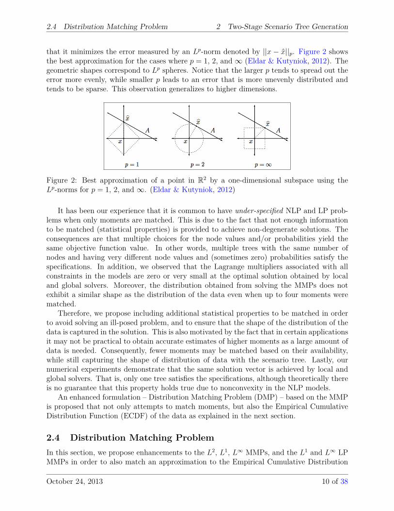
that it minimizes the error measured by an Lp-norm denoted by ||x − x||p. Figure 2 showsthe best approximation for the cases where p = 1, 2, and ∞ (Eldar & Kutyniok, 2012). Thegeometric shapes correspond to Lp spheres. Notice that the larger p tends to spread out theerror more evenly, while smaller p leads to an error that is more unevenly distributed andtends to be sparse. This observation generalizes to higher dimensions.

Figure 2: Best approximation of a point in R2 by a one-dimensional subspace using theLp-norms for p = 1, 2, and ∞. (Eldar & Kutyniok, 2012)

It has been our experience that it is common to have under-specified NLP and LP prob-lems when only moments are matched. This is due to the fact that not enough informationto be matched (statistical properties) is provided to achieve non-degenerate solutions. Theconsequences are that multiple choices for the node values and/or probabilities yield thesame objective function value. In other words, multiple trees with the same number ofnodes and having very different node values and (sometimes zero) probabilities satisfy thespecifications. In addition, we observed that the Lagrange multipliers associated with allconstraints in the models are zero or very small at the optimal solution obtained by localand global solvers. Moreover, the distribution obtained from solving the MMPs does notexhibit a similar shape as the distribution of the data even when up to four moments werematched.

Therefore, we propose including additional statistical properties to be matched in orderto avoid solving an ill-posed problem, and to ensure that the shape of the distribution of thedata is captured in the solution. This is also motivated by the fact that in certain applicationsit may not be practical to obtain accurate estimates of higher moments as a large amount ofdata is needed. Consequently, fewer moments may be matched based on their availability,while still capturing the shape of distribution of data with the scenario tree. Lastly, ournumerical experiments demonstrate that the same solution vector is achieved by local andglobal solvers. That is, only one tree satisfies the specifications, although theoretically thereis no guarantee that this property holds true due to nonconvexity in the NLP models.

An enhanced formulation – Distribution Matching Problem (DMP) – based on the MMPis proposed that not only attempts to match moments, but also the Empirical CumulativeDistribution Function (ECDF) of the data as explained in the next section.

2.4 Distribution Matching ProblemIn this section, we propose enhancements to the L2, L1, L∞ MMPs, and the L1 and L∞ LPMMPs in order to also match an approximation to the Empirical Cumulative Distribution

October 24, 2013 10 of 38


Function (ECDF) of the data. Before describing the steps of the algorithm to incorporatethe ECDF information into the optimization models, some definitions are presented.

For a given random variable (r.v.) Z, the probability of Z to take on a value, say z, lessthan or equal to some value t is given by the Cumulative Distribution Function (CDF), ormathematically CDF (t). A CDF is associated with a specific Probability Density Function(PDF), for continuous r.v.s, or Probability Mass Function (PMF), for discrete r.v.s. In orderto avoid making assumptions about the distribution model, an estimator of the CDF can beused, the Empirical CDF (ECDF), which is defined as follows (van der Vaart, 1998):

ECDF (t) = 1n

N∑i=1

1{zi ≤ t} (7)

where n is the sample size and 1{A} is the indicator function of event A, that takes the valueof one if event A is true, or zero otherwise. Therefore, given a value t, the ECDF returnsthe ratio between the number of elements in the sample that are less than or equal to t andthe sample size.

Every CDF has the following properties:

• It is (not necessarily strictly) monotone non-decreasing;

• It is right-continuous;

• limx→−∞

CDF (x) = 0; and

• limx→+∞

CDF (x) = 1.

We note that most CDFs are sigmoidal. Therefore, the ECDF, as an estimator of the CDF,is also “S-shaped” in most cases. Hence, in order to incorporate the ECDF data in theoptimization models in a smooth way, we propose fitting the Generalized Logistic Function(GLF) (Richards, 1959), also known as Richards’ Curve, or a simplified version (for instance,the Logistic Function is a special case of the GLF). The GLF is defined as follows:

GLF (x) = β0 + β1 − β0

(1 + β2e−β3x)1/β4(8)

where β0, β1, β2, β3, and β4 are parameters to be estimated. When fitting the GLF toECDF data, the GLF can be simplified by setting β0 = 0 and β1 = 1 as these parameterscorrespond to the lower and upper asymptotes, respectively. Analytical expressions for thepartial derivatives of GLF (x) with respect to its parameters can be derived and used to formthe Jacobian matrix for least-squares fitting purposes.

The algorithm for generating a two-stage scenario tree, where the uncertain parametershave no time-series effect, by matching moments and ECDF is described as follows:

Step 1: Collect data for the (independent) uncertain parameters and obtain individualECDF curves for each data set.

Step 2: Approximate each ECDF curve obtained by fitting the Generalized Logistic Func-tion (GLF) or a simplified version.

October 24, 2013 11 of 38


Step 3: Solve a Distribution Matching Problem (DMP) defined in equations (9), (10), or(11).

Remark. We note that if a particular probability distribution family is assumed, i.e. aparametric approach is taken, then CDF information rather than ECDF data can be used inthe DMP. This avoids the extra step of fitting a smooth curve to the ECDF data. However,very few distribution families have closed-form expressions for the CDF. Thus, approximateformulas have to be used in order to avoid evaluating integrals in the DMP.

Extended versions of the three MMP formulations for Step 3 are presented as follows.Note that since ECDF information is taken into account, we must ensure that the values ofthe nodes in the tree are ordered, i.e. order statistics. The convention adopted is the follow-ing: xi,1 ≤ xi,2 ≤ . . . ≤ xi,N, which is ensured via additional inequalities in each extendedNLP model. Because the node values are ordered, the summation ∑j

j′=1 pj′ represents thecumulative probability of the node value xi,j.

(L2 DMP)

minx, p

zL2

DMP = zL2

MMP +∑i∈I

N∑j=1

ωi,jδ2i,j (9a)

s.t.

Constraints (2b) – (2g)

ECDF (xi,j)−j∑

j′=1pj′ = δi,j ∀ i ∈ I, j = 1, . . . , N (9b)

xi,j ≤ xi,j+1 ∀ i ∈ I, j = 1, . . . , N− 1 (9c)

where the variables δi,j represent the deviations with respect to the ECDF data, which in turnare approximated by, for example, the GLF and is represented by the expression ECDF (xi,j).In addition to minimizing the weighted square errors from matching (co-)moments, the sumof squares of the deviations δi,j is also minimized with given weights ωi,j that can be chosenrelative to the weights for the term involving the moments. Thus, the weights represent atrade-off between matching sample (co-)moment data and a smooth representation of the(E)CDF.

October 24, 2013 12 of 38


(L1 DMP)

minx, p

zL1

DMP = zL1

MMP +∑i∈I

N∑j=1

ωi,j(δ+i,j + δ−i,j) (10a)

s.t.

Constraints (3b) – (3i)

ECDF (xi,j)−j∑

j′=1pj′ = δ+

i,j − δ−i,j ∀ i ∈ I, j = 1, . . . , N (10b)

xi,j ≤ xi,j+1 ∀ i ∈ I, j = 1, . . . , N− 1 (10c)

where the variables δ+i,j and δ−i,j represent the positive and negative deviations with respect

to the ECDF data, respectively. The expression ECDF (xi,j) represents the approximationto the ECDF data obtained by, for example, fitting the GLF. The weights to the deviationsare given by ωi,j.

(L1 LP DMP)

minp

zL1

LP DMP = zL1

LP MMP +∑i∈I

N∑j=1

ωi,j(δ+i,j + δ−i,j) (11a)

s.t.

Constraints (5b) – (5h)

ECDF (xi,j)−j∑

j′=1pj′ = δ+

i,j − δ−i,j ∀ i ∈ I, j = 1, . . . , N (11b)

The constant expression ECDF (xi,j) represents the approximation to the ECDF data ob-tained by, for example, fitting the GLF. Note that it is required that the vector of nodevalues is ordered, that is, xi,j ≤ xi,j+1 for j = 1, . . . , N− 1.

October 24, 2013 13 of 38

2.5 Example 1: Uncertain Plant Yield 2 Two-Stage Scenario Tree Generation

(L∞ DMP)

minx, p

zL∞

DMP = zL∞

MMP + ξ (12a)

s.t.

Constraints (3b) – (3i) and (4b) – (4e)

ECDF (xi,j)−j∑

j′=1pj′ = δ+

i,j − δ−i,j ∀ i ∈ I, j = 1, . . . , N (12b)

ξ ≥ ωi,jδ+i,j ∀ i ∈ I, j = 1, . . . , N (12c)

ξ ≥ ωi,jδ−i,j ∀ i ∈ I, j = 1, . . . , N (12d)

xi,j ≤ xi,j+1 ∀ i ∈ I, j = 1, . . . , N− 1 (12e)

(L∞ LP DMP)

minp

zL∞

LP DMP = zL∞

LP MMP + ξ (13a)

s.t.

Constraints (5b) – (5h) and (6b) – (6e)

ECDF (xi,j)−j∑

j′=1pj′ = δ+

i,j − δ−i,j ∀ i ∈ I, j = 1, . . . , N (13b)

ξ ≥ ωi,jδ+i,j ∀ i ∈ I, j = 1, . . . , N (13c)

ξ ≥ ωi,jδ−i,j ∀ i ∈ I, j = 1, . . . , N (13d)

where ξ is a scalar variable that accounts for the maximum deviations in the ECDF infor-mation.

If a parametric approach to the distribution family is taken, then the term ECDF (·) canbe substituted by an exact closed-form expression, represented by CDF (·), or an approxi-mate formula, denoted by CDF (·), and no curve fitting is needed.

The distribution matching method is illustrated in the following motivating example inwhich the objective is to determine the optimal production plan of a network of chemicalfacilities or plants. For simplicity, the only uncertain parameter considered is the productionyield of one facility in the network. The example demonstrates the impact that selecting ascenario tree has on the quality of the solution of the stochastic model.

2.5 Example 1: Uncertain Plant YieldFigure 3 shows the network of the motivating example used throughout the paper. It consistsof a raw material A, an intermediate product B, finished products C and D (only productD can be stored), and facilities (plants) P1, P2, and P3. Product C can also be purchased

October 24, 2013 14 of 38


from a supplier, or in the case of multiple sites, it could be transferred from another sitethat also produces it.

Supply A P1 B

P2

P3

C

D

Purchase

Sales

Sales

Storage

xpurchA,t yrateP1,t wrateP1,t

yrateP2,t

yrateP3,t

wrateP2,t

wrateP3,t

xpurchC,t

xsalesC,t

xsalesD,t

winvD,t

Figure 3: Network structure for the motivating Example 1.

The Linear Programming (LP) formulation has the following main elements: variablescorresponding to the inlet/outlet flow rates to/from facility f in time period t, yratef,t and wrate

f,t

respectively; production yields for each facility, θf ; and demands for each finished productm ∈ FP in time period t, ξm,t. The deterministic multiperiod optimization model is givenas follows:

max wprofit (14a)s.t. wrate

f,t = θfyratef,t ∀ f ∈ F, t ∈ T (14b)

xsalesC,t = wrateP2,t + xpurchC,t ∀ t ∈ T (14c)

winvD,t = winv

D,t−1 + wrateP3,t − xsalesD,t ∀ t ∈ T (14d)

wrateP1,t = yrateP2,t + yrateP3,t ∀ t ∈ T (14e)

xpurchA,t = yrateP1,t ∀ t ∈ T (14f)xsalesm,t + slacksalesm,t = ξm,t ∀ m ∈ FP, t ∈ T (14g)wratef,t ≤ wrate,max

f,t + slackmax,capf,t ∀ f ∈ F, t ∈ T (14h)

wratef,t ≥ wrate,min

f,t − slackmin,capf,t ∀ f ∈ F, t ∈ T (14i)

winvD,t ≤ winv,max

D,t ∀ t ∈ T (14j)xpurchA,t ≤ xpurch,max

A,t ∀ t ∈ T (14k)

where constraints (14b) relate the output flows with the input flows through the yield of eachfacility f , constraints (14c) – (14f) represent material and inventory balances, equations (14g)represent the demand satisfaction and slack variables are employed to account for possibleunmet demand, constraints (14h) – (14k) are limitations in the flows, storage, raw material

October 24, 2013 15 of 38


availability, and capacity violations, respectively, and the profit is calculated as follows:

wprofit =∑t∈T

∑m∈FP

SPm,txsalesm,t −∑f∈F

OPCf,twratef,t −

∑m∈M :MPUR=1

PCm,txpurchm,t −

∑m∈M :MINV=1

ICm,twinvm,t −

∑m∈FP

PENm,tslacksalesm,t −

∑f∈F

PENf,t(slackmax,capf,t + slackmin,cap

f,t )

where SPm,t is the selling price of material m in period t, OPCf,t is the operating cost offacility f in period t, PCm,t is the purchase cost of material m in period t, ICm,t is theinventory cost of material m in period t, and PENm,t denotes the penalty associated withunmet demand.

Consider historical data showing the variability of the production yield of facility P1,θP1, with 120 data points, which represent monthly records of θP1 for a period of ten years.The distribution of θP1 is depicted in a histogram as shown in Figure 4. Only the first twomoments and ECDF data were estimated from the randomly generated production yieldvalues. The simplified GLF (β0 = 0 and β1 = 1) fit to ECDF data and the estimatedparameters are shown in Figure 5. Details of the procedure for generating the historicaldata for θP1, fitting the simplified GLF, and the remaining parameters for the productionplanning model are given in Appendix A.

Figure 4: Distribution of the historical data for the production yield of facility P1.

Figure 5: ECDF data of the production yield of facility P1 fitted by a simplified GLF.

October 24, 2013 16 of 38


To simplify the analysis, we model this multiperiod production planning problem asa Two-Stage Stochastic Programming (TSSP) problem. There are four time periods thatcorrespond to a quarterly production plan problem over the course of one year time horizon.The first stage or here-and-now variables are all the model variables in the model at thefirst time period, t = 1, whereas the second stage or wait-and-see variables are all themodel variables at the remaining time periods, t > 1. All the DMPs and the deterministicequivalent of the TSSP models are implemented in AIMMS 3.13 (Roelofs & Bisschop, 2013).The DMPs were solved with IPOPT 3.10.1 using the Multi-Start Module in AIMMS and theTSSP model was solved with Gurobi 5.1. The model sizes are small; therefore, CPU timesare not reported. In the DMPs, the yield variables were bounded below by the minimumdata point, and above by the maximum data point.

Five scenarios are selected for the two-stage scenario tree. Two approaches are compared:heuristic and DMP, which includes the optimization models described in Subsection 2.4. Theheuristic approach represents an arbitrary way to construct a scenario tree that does notconsider the distribution of the historical data. From minimum and maximum data values(e.g., production yield that can vary between 0 and 1), their arithmetic mean is calculated(center node) and the values of the other nodes are calculated by fixed deviations of ±20%and ±40% from the mean node. Therefore, the tree in this example has five nodes in thesecond stage. Also, the probabilities are arbitrarily chosen. Notice that by not visualizing thedistribution of the uncertain parameter, choice of outcomes and their probabilities may notsatisfactorily characterize the shape of the distribution of the actual data. In other words,the heuristic scenario tree does not represent the actual problem data and the productionplan obtained may not be very meaningful. The DMP approach calculates the probabilities(both LP and NLP formulations) and values of the nodes (only NLP formulations) in order tomatch statistical properties that describe the distribution of the yield data. The targets forthe DMPs include the first two moments and ECDF data. Figure 6 shows the probabilitiesand yield values obtained for the five-scenario tree in each approach.

October 24, 2013 17 of 38


Figure 6: Probability profiles for the heuristic and optimization-based (DMP) approaches inExample 1. For reference, a histogram of the uncertain data is depicted in Figure 4.

Note that despite attempting to match only the first two moments, the additional ECDFinformation allows for the probability profiles obtained by solving the L2 DMP, L1 DMP andL∞ DMP formulations to satisfactorily capture the shape of the distribution of the uncertainparameter. The yield distribution as shown in Figure 4 is skewed to the right, which resultsin higher probabilities assigned to node values that are slightly higher than the mean yield(0.7301). Such characteristic is not captured in the heuristic approach. Thus, it does notsatisfactorily represent the actual data. It was observed that the probabilities obtained withthe L1 LP DMP and L∞ LP DMP formulations were strongly dependent on the node valueschosen and this fact will affect the remaining results shown below. The objective functionvalue of the three DMP formulations are shown in Table 1. Note that the extra degrees offreedom associated with considering the node values as variables (NLP formulations) resultedin smaller deviations in the matching procedure for the choices of weights (see Appendix A).

Table 1: Objective function values of the DMP formulations in Example 1. The valuesrepresent the error of matching the statistical properties.

Model Objective FunctionL2 DMP 0.0081L1 DMP 0.1453

L1 LP DMP 0.5200L∞ DMP 0.0918

L∞ LP DMP 0.2317

Table 2 shows the optimal expected profit of the stochastic production planing modelin equation (14). The relatively low expected profit by using the heuristic approach can

October 24, 2013 18 of 38


be explained due to high probabilities placed on production yields below the mean of theactual yield data. In other words, the scenario tree in the heuristic approach is pessimisticfor the values chosen for the production yield of facility P1. Ultimately, the tree in theheuristic approach is an inaccurate representation of the yield data. However, note thatthe magnitude of the expected profit of the TSSP problem is not an assessment of thequality of each solution with respect to the “true” solution that would be obtained if thetrue distributions were known and were not approximated by finite discrete outcomes. TheLP deterministic equivalent two-stage stochastic program has 273 constraints, 305 variables,832 nonzeros, and was solved in not more than 0.02 seconds for all approaches.

Table 2: Expected profit of the production planning model in Example 1 using the scenariotrees from two approaches.

Approach Expected Profit [$]Heuristic 65.43L2 DMP 73.23L1 DMP 73.70

L1 LP DMP 76.48L∞ DMP 77.05

L∞ LP DMP 76.39

Figures 7 and 8 show the different production plans obtained for each approach. Specif-ically, the solution obtained with the heuristic approach predicted higher overall inventorylevels of product D for the time horizon under consideration. Moreover, using the tree ob-tained with the heuristic approach incurred higher purchase amounts of product C in everyperiod in the time horizon, which can explained by the fact that the scenario tree in thatapproach is constructed around a lower mean than the actual mean estimated from the data.

Figure 7: Optimal inventory levels of product D from using the scenarios obtained fromheuristic and DMP approaches.

October 24, 2013 19 of 38


Figure 8: Optimal purchase amounts of product C from using the scenarios obtained fromheuristic and DMP approaches.

Finally, the quality of the stochastic solutions was assessed using a simulation-basedMonte Carlo sampling scheme that provides statistical bounds on the optimality gap (Bayrak-san & Morton, 2006). The optimality gap is defined as the difference between an approx-imation of the “true” stochastic solution (very large tree to approximate the continuousdistribution of the yield) and the candidate stochastic solution. In this context, a candidatestochastic solution refers to the first-stage decisions of the TSSP when using the scenariotrees from either heuristic or DMP approaches. The Multiple Replications Procedure (MRP)was used with twenty replications, and each replication contains one hundred independentscenarios. In each replication, the gap between the approximate true solution and the candi-date solution is calculated. Table 3 shows the average gap of all replications plus one-sidedconfidence intervals for 95% confidence. The results suggest that the stochastic productionplanning solutions obtained by using the trees generated by the L2 DMP and L1 DMP ap-proaches are closer to the true solution as seen from the small optimality gap. Note thatsince the historical data were artificially generated, i.e. the data-generating mechanism(distribution) is known (see Appendix A), a Monte Carlo sampling strategy can be used.

Table 3: Average value and upper bound of the optimality gap of the stochastic productionplanning model in Example 1.

Approach Avg Gap [$] Upper Bound [$]Heuristic 0.21 0.29L2 DMP 0.04 0.10L1 DMP 0.04 0.11

L1 LP DMP 0.70 0.91L∞ DMP 0.37 0.50

L∞ LP DMP 0.70 0.91

The results in Table 3 clearly show that selecting the scenario tree as an input to thestochastic optimization model is crucial to obtain a meaningful solution of an SP formula-tion. The distribution matching method is a scenario generation method that allows creating

October 24, 2013 20 of 38

2.6 Reducing the Scenario Tree 3 Multi-Stage Scenario Tree Generation

scenario trees that satisfactorily represent the distribution of the data, so that the decisionsmade with the stochastic optimization model are supported by factual probabilistic infor-mation.

2.6 Reducing the Scenario TreeTwo methods have been commonly used in the literature to remove scenarios by aggregatingneighboring nodes in a scenario tree. The scenario reduction method, originally proposedby Dupačová, Gröwe-Kuska, & Römisch (2003), and later improved by Heitsch & Römisch(2009), is a heuristic that attempts to generate a tree with pre-specified number of scenariosthat is the closest to the “original” distribution according to a probability metric. Theintuitive idea is to find a subset of the original set of scenarios of prescribed cardinalitythat has the shortest distance to the remaining scenarios. Feng & Ryan (2013) modifiedthat method to also account for what the authors call “key” first-stage decisions in theaggregation of scenarios in addition to probability metrics.

Another common approach to reduce the number of scenarios comes from clusteringmethods in data mining (Hastie, Tibshirani, & Friedman, 2009). In particular, some authorshave used variants of the k-means clustering algorithm, where the main goal is to group oraggregate paths in the scenario tree that are “near” to each other according to some distancemetric that is minimized. For instance, Xu, Chen, & Yang (2012) proposed a k-meansalgorithm that generates a scenario tree from a fan-like tree that not only groups paths thatare near in a probabilistic sense, but also accounts for inter-stage dependency of the data.

3 Multi-Stage Scenario Tree GenerationThe MMPs in equations (2) – (6) and DMPs in equations (9) – (13) can be applied to bothtwo-stage and multi-stage cases. When generating multi-stage scenario trees, a statisticalproperty matching problem is solved at every node of the tree except at the leaf or terminalnodes. Multi-stage scenario trees can be viewed as a group of two-stage subtrees that areformed by branching out from every node except the leaf nodes. The complication in gener-ating multi-stage scenario trees with interstage dependency lies in the fact that the momentscalculated for each path into future stages are dependent on the previous states or nodespresent in each path. Therefore, prediction of future events (time series forecasting) mustbe combined with property matching optimization as will be described below.

For stochastic processes, such as time-series data of product demands, statistical proper-ties can be estimated through forecasting models that take into account information that isconditional on past events. Appendix ?? contains more details of using time series forecastingmodels to estimate the statistical properties.

Time series forecasting models play an essential role in generating scenario trees whenthere is a time-series effect in the uncertain parameters. Briefly, mathematical models arefit to the historical data and their predictive capabilities provide conditional (co-)momentsof the uncertain parameters at future stages. The moments are conditional on past events.That is, they take into account the serial dependency of the time-stamped observed valuesof the uncertain parameters. Hence, the statistical moments are supplied to the property

October 24, 2013 21 of 38

3.1 NLP Approach 3 Multi-Stage Scenario Tree Generation

matching optimization models at each non-leaf node and the scenario tree is consistentlygenerated. Moreover, simulation of the time series models can be used to generate data ofwhich an ECDF can be constructed and approximated with a smooth function, such as theGLF or a simplified version (see Subsection 2.4).

In the next two sections, we present two sequential solution strategies for generating amulti-stage scenario tree: NLP Approach and LP Approach. We focus on the DMP formu-lations, where L2 DMP, L1 DMP and L∞ DMP are nonlinear (both node values and proba-bilities are variables), whereas L1 LP DMP and L∞ LP DMP are linear (only probabilitiesare variables). Each approach comprises two main steps, forecasting and optimization,which are summarized below:

Forecasting Step: After successfully fitting a time series model to the data, forecast futurevalues.

• Input: observed data represented by the nodes• Output: conditional moments and ECDF information to be matched in the opti-

mization step

Optimization Step: Solve a DMP at a given node in the tree.

• Input: conditional moments estimated by the forecasting step• Output: probabilities of outcomes, and if using the NLP approach, values of the

nodes

Remark 1. Conditional (co-)moments are readily available via forecasting. ECDFinformation can be obtained through simulation of time series models, and a brief overviewis given in ?? in Appendix ??. If a particular family of distribution is assumed for theforecast data, then the CDF or an approximate expression can be used instead as illustratedin Example 2 (Subsection 3.3).

Remark 2. Instead of a forecasting step, some authors have used a simulation step togenerate the targets (conditional moments) to the optimization step and/or the values ofthe nodes in the scenario tree. For example, Høyland, Kaut, & Wallace (2003) proposeda heuristic method to produce a discrete joint distribution of the stochastic process thatis consistent with specified values of the first four marginal moments and correlations. Inaddition, due to the independence of the optimization problems to be solved at each node ofa given stage, there is an opportunity for parallel algorithms to speed up the solution process(Beraldi, De Simone, & Violi, 2010).

3.1 NLP ApproachA general solution strategy for generating a multi-stage scenario tree using the NLP formu-lations of the DMP consists of alternating the two main steps described above in a shrinking-horizon fashion, i.e. marching forward in time, node-by-node and stage-by-stage until theend of the time horizon. Figure 9 depicts the sequence of steps in the approach. The blackdots (past region) in each subfigure correspond to historical data of the uncertain parameterunder consideration, the blue line represents the time series model used to make predictions

October 24, 2013 22 of 38

3.1 NLP Approach 3 Multi-Stage Scenario Tree Generation

of the stochastic process, the red dots (future region) are the possible future states thatthe stochastic process will visit, and the grey shaded area surrounding the red dots denotesthe estimated prediction confidence limits for a given significance level of α, i.e. α = 0.05indicates 95% confidence. Note that by connecting parent nodes to their descendants (fromleft to right), a scenario tree is obtained.

The algorithm can be stated as follows.

Step 0: Start at the root (“present”) node whose value is known. Set it as the current node.

Step 1: If not the last stage in the time horizon, then perform a one-step-ahead forecastfrom the current node to estimate conditional moments.

Step 2: Simulate the time series model including observations up to the current node, con-struct the ECDF curve, and approximate it by a smooth function, such as the GLFor a simplified version.

Step 3: Solve a nonlinear DMP to determine the node values and their probabilities for thenext stage.

Step 4: For each node determined, set it as the current node and go to Step 1.

In Figure 9, the blue curve represents the time series model, the black dots representpast or historical data, the green dot is the current or present state, and the red dots arethe future states. For demonstration purposes, Figure 9(c) only shows the forecasting stepfor the bottom node generated in the first optimization step. Note that some nodes may lieoutside the confidence interval predicted by the forecasting step; this allows more extremeevents to be captured in the scenario tree, which in turn subject the stochastic programmingproblem to riskier scenarios and may lead to more “robust” solutions.

October 24, 2013 23 of 38

3.2 LP Approach 3 Multi-Stage Scenario Tree Generation

(a) First one-step-ahead forecasting step to predict the most likely value of the stochastic processin the next stage as well as possible higher moments and distribution information from simulation.

(b) Optimization step to calculate probabilities and nodes for the next stage. Optionally, the nodecorresponding to the conditional mean may be fixed in the DMP.

(c) One-step-ahead forecasting step from a given node obtained in the optimization step before.Repeat these steps for every node generated in every stage until the end of the time horizonconsidered.

Figure 9: Alternating forecasting and optimization steps in generating multi-stage scenariotrees using the NLP Approach. CI denotes the confidence interval estimated at each forecastand ECDF means Empirical Cumulative Distribution Function.

The complexity in implementing this approach in practice is the communication betweenthe forecasting and the optimization steps at every non-leaf node in the tree. On the otherhand, the approach using the LP formulations of the property matching problems onlyalternates between the forecasting and optimization steps once. The next section containsour proposed approach, and we note that there are variants in the literature that for instanceuse clustering algorithms as discussed in Subsection 2.6.

3.2 LP ApproachThe only decision variables in the LP formulation in equation (11) are the probabilities ofthe outcomes. Therefore, if the node values are known in advance, then a single optimizationproblem can be solved for the entire tree to compute their probabilities. Thus, the approachhas only two steps: (1) the forecasting step generates the nodes plus the statistical propertiesto be matched, and (2) an LP DMP is solved for all non-leaf nodes simultaneously. The

October 24, 2013 24 of 38

3.2 LP Approach 3 Multi-Stage Scenario Tree Generation

optimization step is a straightforward solution of an LP problem, whereas the forecastingstep contains elements that are particular to a specific strategy.

The strategy for the forecasting step proposed in this paper is shown in Figure 10. Asshown in Figure 10(a), after performing a one-step-ahead forecast from the present node tothe base or most likely node in the second stage, additional nodes are created by adding andsubtracting multiples of the standard error of the forecast to the base node. The numberof additional nodes above and below the base node is chosen a priori. In practice, near-future stages may be more finely discretized than far-future stages, since the prediction isless accurate the further into the future it is made. For ease of exposition, Figure 10(b)shows the forecast from the second to the third stage of one of the nodes created in thesecond stage. The process is repeated for every node in every stage, except the last one ofthe time horizon considered.

(a) First one-step-ahead forecasting step to predict the most likely value of the stochastic processin the next stage. Create new nodes by adding and subtracting multiples of the standard error, σe,of the forecast to the base node.

(b) For each node created, perform a one-step-ahead forecast and create new nodes. Repeat theprocess until the end of the time horizon considered.

Figure 10: Proposed forecasting step in generating multi-stage scenario trees using the LPApproach. σe, CI, and ECDF denote the standard error, confidence interval estimated ateach forecast, and the Empirical Cumulative Distribution Function, respectively.

In summary, the main difference between the NLP Approach and the LP Approach isthat, in the latter, the forecasting and optimization steps alternate only once as all the nodesor outcomes of the tree are created in the forecasting step, and then the optimization stepis executed to compute the probabilities.

The next example demonstrates how the two approaches can be used to generate a multi-stage scenario tree when product demand is uncertain.

October 24, 2013 25 of 38

3.3 Example 2: Uncertain Product Demands 3 Multi-Stage Scenario Tree Generation

3.3 Example 2: Uncertain Product DemandsConsider the same network depicted in Figure 3 and the deterministic multiperiod productionplanning model defined in (14). In this case, the product demands of C and D are theuncertain parameters. The planning horizon is one year, which is divided into time periodsof quarters. Quarterly historical demand data are given from the years of 2008 to 2012. Thus,the frequency (number of observations per year) of the time series is four. The objectiveis to obtain the optimal quarterly production plan for the year of 2013. As in Example 1,all optimization models were implemented in AIMMS 3.13. The NLP problems were solvedwith IPOPT 3.10.1 using the multi-start module in AIMMS with 30 sample points and 10selected points in each iteration. All LP models were solved with CPLEX 12.5. In the DMPs,the demand variables were bounded below by half the minimum and above by double themaximum historical demand data points.

A common approach for deciding the structure of multi-stage trees is to select moreoutcomes per node in earlier stages than in later stages, since the uncertainty in the forecastsis much higher in the latter. Thus, it is more reasonable to select a finer discretization inearlier stages. It is then decided that the multi-stage scenario tree has the following structure:1-5-3-1, which means that the second quarter has five outcomes, the third quarter has treeoutcomes for each outcome in the second quarter, and the fourth quarter has only oneoutcome for each outcome of the third quarter, thus, the scenario tree has 15 scenarios asseen in Figure 11. As in Example 1, a heuristic approach is compared with the optimization-based DMPs to obtain scenario trees. We consider uncertainty in the demand of bothproducts C and D. The tree for each individual product demand is obtained as follows. Thecenter or base node at a given quarter is the arithmetic average of the corresponding quarterof previous years, and the remaining nodes above and below the base node are obtained byfixed deviations. Therefore, the node values ignore the serial dependence and time-serieseffects in the data. The individual heuristic trees for products C and D were combined intoa single tree with the same structure (1-5-3-1) by overlapping the outcomes for each stageas shown in Figure 11. Probabilities of outcomes were arbitrarily chosen and are symmetricwith respect to each base node.

October 24, 2013 26 of 38


Figure 11: Heuristic scenario tree for the demand of products C and D. The percentagedeviations are computed based on each base node. The values above and below the arcs arearbitrarily chosen probabilities.

Figure 12 shows the time series demand data for products C and D. The time seriesmodel that best fits the data (see Appendix B for details) is fixed in subsequent forecasts.That is, when executing an approach no refitting is performed prior to forecasting. The rootnode of the tree, which is the node value at the first quarter in 2013 or “Q12013”, is forecastand assumed to have probability of one. The constant variance for the demand of productsC and D are estimated to be 1.65 t2 and 1.14 t2, respectively, and the properties matchedare first two moments, covariance, and CDF information.

Figure 12: Time series data of the demand of products C and D.

Since the demand data are fitted to a linear Gaussian model (ARIMA), the forecastsare expected to follow normal distributions. Therefore, an expression for the CumulativeDistribution Function (CDF) of a normal distribution with mean µ and standard deviation

October 24, 2013 27 of 38


σ can be used in the constraints involving ECDF (·). In particular, the CDF of a normaldistribution can be written in terms of the error function as follows (Abramowitz & Stegun,1965):

CDF (x)Normal := Φ(x− µσ

)= 1

2

[1 + erf

(x− µσ√

2

)]where erf(·) is the error function defined as the following integral:

erf(x) = 2√π

∫ x

0e−t

2dt

Hence, constraints (9b) can be replaced with,

Φxi,j −Mi,1√

Mi,2

− j∑j′=1

pj′ = δi,j ∀ i ∈ I, j = 1, . . . , N

constraints (10b) and (12b) can be substituted by,

Φxi,j −Mi,1√

Mi,2

− j∑j′=1

pj′ = δ+i,j − δ−i,j ∀ i ∈ I, j = 1, . . . , N

and finally constraints (11b) and (13b) are rewritten as,

Φxi,j −Mi,1√

Mi,2

− j∑j′=1

pj′ = δ+i,j − δ−i,j ∀ i ∈ I, j = 1, . . . , N

AIMMS offers a native, numerical approximate implementation of the error function, whichcan be directly used in the implementation of the constraints in the DMPs.

Exclusively for the LP DMPs, it was observed that additional constraints on the probabil-ities were necessary in order to enforce a normal-like profile, i.e. probabilities monotonicallydecrease from the center node outward. The additional constraints are given below and areequivalent to the ones proposed by Ji et al. (2005).

pj ≥ pj′ ∀ j =⌈N2

⌉, . . . , N, j′ > j

pj ≥ pj′ ∀ j = 1, . . . ,⌈N2

⌉, j′ < j

For illustration purposes, the scenario trees obtained with NLP and LP approaches areshown in Figure 13 (L2 DMP) and Figure 14 (L∞ LP DMP), respectively. For the NLPApproach, the node values in the fourth time period correspond to the conditional meansobtained via forecasting, i.e. no optimization was needed as only one outcome was consid-ered. It should be noted that the total time for solving the six NLPs with multi-start forthe tree in Figure 13 was 12.35 seconds, while the LP in Figure 14 took 0.02 seconds.

October 24, 2013 28 of 38


14.3617.36

13.0516.15

12.5816.22

12.7716.70

0.33

13.9317.33

13.9017.14

0.40

15.8818.96

15.5517.78

0.27

0.18

13.9816.92

13.3916.53

13.4416.83

0.34

14.7317.64

14.5817.26

0.40

16.6919.28

16.2417.91

0.26

0.24

14.8117.61

14.1016.81

14.0516.94

0.34

15.4517.93

15.1917.38

0.40

17.4219.56

16.8618.02

0.26

0.25

15.7618.41

14.9217.13

14.7417.06

0.34

16.2718.25

15.8917.50

0.40

18.2419.89

17.5618.15

0.26

0.21

17.3219.70

16.2617.65

15.8817.27

0.35

17.6218.78

17.0317.71

0.40

19.6020.43

18.7018.36

0.25

0.12

Figure 13: Scenario tree obtained with the NLP Approach (L2 DMP) for Example 2. Topand bottom values inside each node are the calculated demands of products C and D,respectively.

14.3617.36

11.7015.02

10.6515.10

11.1316.26

0.32

12.0216.23

12.2916.71

0.36

13.3817.37

13.4417.16

0.32

0.05

12.9816.09

11.8215.59

12.1216.46

0.33

13.1016.65

13.2016.88

0.34

14.3917.72

14.2917.29

0.33

0.29

14.2717.15

12.9416.03

13.0616.63

0.33

14.1917.07

14.1217.04

0.34

15.4418.11

15.1817.45

0.33

0.34

15.5518.22

13.9916.42

13.9616.79

0.33

15.2717.49

15.0417.20

0.34

16.5618.56

16.1317.62

0.33

0.26

16.8319.29

14.9916.77

14.8016.92

0.32

16.3617.91

15.9617.37

0.36

17.7319.05

17.1217.82

0.32

0.06

Figure 14: Scenario tree obtained with the LP Approach (L∞ LP DMP) for Example 2. Thenode values are obtained via forecasting and the probabilities are calculated via optimization.Top and bottom values in each node are the demands of products C and D, respectively.

The optimal expected profit of the production planning model by using the scenario

October 24, 2013 29 of 38


tree of the proposed approach as the input, and by solving the deterministic equivalent ofthe multi-stage stochastic programming model is shown in Table 4. The heuristic approachunderestimates the expected total profit when compared to the NLP DMPs. Again, wenote that the scenario probabilities and the solution obtained with the LP DMPs is greatlyaffected by the node values chosen. The LP deterministic equivalent of the multi-stagestochastic program has 613 constraints, 685 variables, 1,872 nonzeros, and was solved in lessthan 0.02 seconds for all approaches.

Table 4: Expected profit in Example 2 using the scenario trees from heuristic andoptimization-based approaches.

Approach Expected Profit [$]Heuristic 79.95L2 DMP 82.39L1 DMP 82.65

L1 LP DMP 80.04L∞ DMP 82.41

L∞ LP DMP 80.03

Figures 15 and 16 show the different production plans obtained for each approach ateach quarter. Specifically, the solution obtained with the heuristic approach predicted higheroverall inventory levels of product D for the time horizon under consideration. Moreover,the solution using the heuristic tree shows very different average flowrates out of plant P2compared to the ones obtained using the DMP formulations. In real life terms, the productionquota for a plant affects lower-level operability decisions, such as scheduling and control.

Figure 15: Optimal inventory levels of product D from using the scenarios obtained fromheuristic and DMP approaches.

October 24, 2013 30 of 38


Figure 16: Optimal flow rates out of plant P2 from using the scenarios obtained fromheuristic and DMP approaches.

Finally, similarly to Example 1, the quality of the stochastic solutions was assessed usinga simulation-based Monte Carlo sampling scheme that provides statistical bounds on theoptimality gap (Chiralaksanakul & Morton, 2004). The optimality gap is calculated using atree-based estimator of the lower bound (candidate solution, maximization problem) and theapproximate true solution (upper bound estimator, maximization problem). The simulatedtrees have the structure 1-10-10-10, which amounts to one thousand scenarios. All subtreesare generated by simulating ARIMA processes (see ?? in Appendix ??). Ten replicationsof the algorithm (see Procedure P2 in the original paper) were performed to obtain theconfidence interval on the gap. Table 5 shows the one-sided confidence intervals for 95%confidence. Note that by modeling the demand time series as ARIMA processes, the data-generating mechanism is known, and Monte Carlo sampling can be performed by simulatingthe ARIMA models (see ?? in Appendix ??).

Table 5: Average value and upper bond of the optimality gap of the stochastic productionplanning model in Example 2.

Approach Avg Gap [$] Upper Bound [$]Heuristic 2.03 2.16L2 DMP 0.92 1.00L1 DMP 0.93 1.01

L1 LP DMP 1.12 1.35L∞ DMP 0.93 1.01

L∞ LP DMP 1.04 1.22

Note that the confidence interval of the gaps obtained for all the DMP formulations arelower than the one obtained for the heuristic approach, which indicates that the scenariotrees generated via the optimization-based procedure are good approximations of the “true”distribution. In addition, they contain correlation information between the demands of thetwo products, thus improving the characterization of the uncertainty.

October 24, 2013 31 of 38

4 Conclusions

4 ConclusionsIn this paper, we have described a systematic method for scenario tree generation that canbe used in optimization and simulation solution strategies in Process Systems Engineering(PSE) problems. The distribution matching method is based on an optimization model thatcan be used to calculate the probabilities and values of outcomes in a scenario tree. Thisis accomplished by attempting to match statistical properties, such as (co-)moments andEmpirical Cumulative Distribution Function (ECDF) information, calculated from the treeto the ones estimated from the data. The motivation behind this approach is to ensurethat the scenarios considered in a stochastic programming framework correspond to thebehavior observed in historical and forecast data, as opposed to assigning arbitrary valuesand probabilities to the nodes in the scenario tree. Therefore, characterizing the uncertaintyadds value to the solution of the stochastic model used for decision-making.

For multi-stage scenario tree generation, we presented two approaches that can be usedin conjunction with time series forecasting or simulation. The NLP Approach is composed oftwo alternating steps: the forecasting or simulation step computes conditional (co-)momentsand ECDF information to be matched, and the optimization step determines the probabilitiesand values of the outcomes in order to match those properties. The two steps are alternateduntil the prescribed time horizon is completed. The LP Approach also contains the sametwo steps, but each step is performed only once. First, the forecasting or simulation stepgenerates all the nodes in the tree and computes the conditional (co-)moments and ECDFinformation, and then the optimization step calculates the probabilities of outcomes.

The quality of the solution of the stochastic programming problems was assessed viasimulation-based Monte Carlo sampling methods. It was shown that the proposed scenariotree generation methods provide good-quality solutions, and provide a systematic approachfor handling multiple sources of uncertainty, thus generating more compact trees with co-variance or correlation information.

AcknowledgmentThe authors gratefully acknowledge financial support from The Dow Chemical Company.They also are grateful to Alex Kalos for the fruitful discussions regarding the incorporationof (E)CDF information to the moment matching method, and to the Advanced Analyticsteam, especially Joe Czyzyk, with regards to time series modeling and forecasting.

Appendix A Data for Example 1The production yield data were randomly generated using the R programming languageversion 3.0.1 (R Core Team, 2013). In particular, the library PearsonDS (Becker & Klößner,2013) was used to generate 120 random numbers sampled from a Pearson distribution withgiven mean, variance, skewness, and kurtosis. The four moments of the generated data werecalculated using functions of the library e1071 (Meyer et al., 2012). The code in Listing A.1can be used to reproduce the yield data in Example 1.

October 24, 2013 32 of 38

APPENDIX A DATA FOR EXAMPLE 1 4 Conclusions

library ( PearsonDS )library (e1071)moments <- c(mean =0.7 , variance =0.02 , skewness =-1, kurtosis =4)set.seed (1234)v <- rpearson (10*12, moments = moments )data.min <- min(v)data.max <- max(v)data.mean <- mean(v)data.var <- var(v)data.dskew <- skewness (v)* data.var ^1.5 # Denormalized skewnessdata.dkurt <- ( kurtosis (v) + 3)* data.var ^2 # Denormalized kurtosis

Listing A.1: R code to generate production yield data and their moments for Example 1.

Only the first two moments and the ECDF information were considered in the DMPs.The weights for the moments were chosen such that the weight of the mean is the same asthe weight of the variance, that is wi,k = 1.0/M2

i,k and wi,k = 1.0/|Mi,k| for L2 DMP andL1 DMP, respectively. The weights for the deviations from the approximation to the ECDFare equal to one, ωi,j = 1.0. The ECDF data were estimated in MATLAB (The MathWorksInc., 2013) with the function ecdf and a simplified GLF (β0 = 0 and β1 = 1) was fit to theECDF data by using the function lsqcurvefit with the following options: 10,000 maximumfunction evaluations (MaxFunEvals), 10,000 maximum iterations (MaxIter), 10−12 functiontolerance (TolFun), exact Jacobian. Initial guesses for the parameters β2, β3, and β4 were100, 10, and 1, respectively.

The parameters for the production planning LP model are given in the following tables.

Table A.1: First-stage production yield (θf at t = 1) [-]. For facilities P2 and P3, the yieldsremain the same at the second stage.

Facility GroupP1 0.85P2 0.7P3 0.9

Table A.2: Product demand (ξm,t) [t].

Product Time Period1 2 3 4

C 20 10 15 17D 15 7 12 10

October 24, 2013 33 of 38

APPENDIX A DATA FOR EXAMPLE 1 4 Conclusions

Table A.3: Maximum inventory (winv,maxm,t ) [t].


D 6 6 6 6

Table A.4: Maximum (minimum) capacity (wminm,t and wmax

m,t ) [t].

Facility Time Period1 2 3 4

P1 20 (5) 20 (5) 20 (5) 20 (5)P2 18 (0) 18 (0) 18 (0) 18 (0)P3 19 (2) 19 (2) 19 (2) 19 (2)

Table A.5: Selling price (SPm,t) [$/t].


C 1.75 1.75 1.71 1.71D 1.10 1.10 1.18 1.18

Table A.6: Operating cost (OPCf,t) [$/t].

Facility Time Period1 2 3 4

P1 0.26 0.26 0.14 0.14P2 0.16 1.16 0.13 0.13P3 0.32 0.32 0.32 0.32

Table A.7: Purchase cost (PCm,t) [$/t].


A 0.05 0.05 0.05 0.05C 1.00 1.00 1.00 1.00

Table A.8: Inventory cost (ICm,t) [$/t].


D 0.03 0.03 0.03 0.03

October 24, 2013 34 of 38

APPENDIX B DATA FOR EXAMPLE 2 References

Table A.9: Raw material availability (xpurch,maxA,t ) [t].

Raw Material Time Period1 2 3 4

A 30 25 27 23

The penalties for unmet demand (PENm,t), and maximum capacity and minimum ca-pacity violations (PENf,t) are 10 times the selling prices, and proportional to the operatingcosts, respectively.

Appendix B Data for Example 2Time series modeling and forecasting were implemented in the R programming language (RCore Team, 2013). For demonstration purposes, only ARIMAmodels (see Appendix ??) werefit to the time series data. The library used for fitting ARIMA models is called forecast(Hyndman et al., 2013). In particular, the function auto.arima was used to automaticallydetermine the best ARIMA model that fits the data according to the default informationcriterion (Akaike Information Criterion, AIC). Seasonality effects were allowed and no holdout sample was considered in the fitting process. The time series demand data for bothproducts C and D were then modeled as ARIMA(1,0,0) processes with non-zero means.Future values were predicted with 95% level of confidence using the predict function in thestats library, which is part of R.

The constant variance of ARIMA models was estimated by the sigma2 attribute of theARIMA object. For the LP Approach in Subsection 3.2, the standard error of a forecastwas estimated by setting the value of the argument se.fit of the predict function to TRUE.Covariance information was estimated through R’s builtin function ccf, which estimates thecross-covariance function of two time series data at different lags. Since the NLP Approachinvolves alternating one-step-ahead forecasting with optimization, the estimated covariancecorresponds to the lag 1 outcome of function ccf.

The parameters for the production planning LP model are the same as the data given intables Tables A.3 to A.9. In addition, the production yield for all time periods are the sameas those given in Table A.1. The product demand for every stage in each scenario tree isgenerated as described in Subsection 3.3.

ReferencesAbel, O., and Marquardt, W. 2000. Scenario-Integrated Modeling and Optimization ofDynamic Systems. AIChE Journal. 46(4):803–823.

Abramowitz, M., and Stegun, I. A. 1965. Handbook of Mathematical Functions: with For-mulas, Graphs, and Mathematical Tables. Dover Publications.

Bartlett, R. 2013. A Practitioner’s Guide to Business Analytics: Using Data AnalysisTools to Improve Your Organization’s Decision Making and Strategy. The McGraw-HillCompanies.

October 24, 2013 35 of 38

REFERENCES References

Bayraksan, G., and Morton, D. P. 2006. Assessing Solution Quality in Stochastic Programs.Mathematical Programming. 108(2-3):495–514.

Becker, M., and Klößner, S. 2013. PearsonDS: Pearson Distribution System. R packageversion 0.95.

Ben-Tal, A.; Ghaoui, L. E.; and Nemirovski, A. 2009. Robust Optimization. Princeton Seriesin Applied Mathematics.

Beraldi, P.; De Simone, F.; and Violi, A. 2010. Generating Scenario Trees: A ParallelIntegrated Simulation-Optimization Approach. Journal of Computational and AppliedMathematics. 233(9):2322–2331.

Birge, J. R., and Louveaux, F. 2011. Introduction to Stochastic Programming. Springer,second edition.

Chen, Y.; Adams II, T. A.; and Barton, P. I. 2011. Optimal Design and Operation ofFlexible Energy Polygeneration Systems. Industrial & Engineering Chemistry Research.50(8):4553–4566.

Chiralaksanakul, A., and Morton, D. P. 2004. Assessing Policy Quality in Multi-stageStochastic Programming. Stochastic Programming E-Print Series. (12):1–36. Retrievedfrom http://edoc.hu-berlin.de/docviews/abstract.php?id=26770.

Colvin, M., and Maravelias, C. T. 2009. Scheduling of Testing Tasks and Resource Planningin New Product Development using Stochastic Programming. Computers & ChemicalEngineering. 33(5):964–976.

Dantzig, G. B. 1955. Linear Programming under Uncertainty. Management Science. 1(3-4):197–206.

Davenport, T. H., and Harris, J. G. 2007. Competing on Analytics: The New Science ofWinning. Harvard Business School Press.

Dupačová, J.; Gröwe-Kuska, N.; and Römisch, W. 2003. Scenario Reduction in Stochas-tic Programming: An Approach using Probability Metrics. Mathematical Programming:Series A. 95:493–511.

Eldar, Y. C., and Kutyniok, G. 2012. Compressed Sensing: Theory and Applications.Cambridge University Press.

Feng, Y., and Ryan, S. M. 2013. Scenario Construction and Reduction Applied to StochasticPower Generation Expansion Planning. Computers & Operations Research 40(1):9–23.

Goel, V., and Grossmann, I. E. 2006. A Class of Stochastic Programs with Decision Depen-dent. Mathematical Programming. 108(2-3):355–394.

Guillén, G.; Espuña, A.; and Puigjaner, L. 2006. Addressing the Scheduling of ChemicalSupply Chains under Demand Uncertainty. AIChE Journal. 52(11):3864–3881.

October 24, 2013 36 of 38

http://edoc.hu-berlin.de/docviews/abstract.php?id=26770


Gülpınar, N.; Rustem, B.; and Settergren, R. 2004. Simulation and Optimization Approachesto Scenario Tree Generation. Journal of Economic Dynamics and Control. 28(7):1291–1315.

Gupta, V., and Grossmann, I. E. 2012. Modeling and Computational Strategies for OptimalDevelopment Planning of Offshore Oilfields under Complex Fiscal Rules. Industrial &Engineering Chemistry Research. 51(44):14438–14460.

Hastie, T.; Tibshirani, R.; and Friedman, J. 2009. The Elements of Statistical Learning:Data Mining, Inference, and Prediction. Springer Series in Statistics, second edition.

Heitsch, H., and Römisch, W. 2009. Scenario Tree Reduction for Multistage StochasticPrograms. Computational Management Science. 6(2):117–133.

Høyland, K., and Wallace, S. W. 2001. Generating Scenario Trees for Multistage DecisionProblems. Management Science. 46(2):295–307.

Høyland, K.; Kaut, M.; and Wallace, S. W. 2003. A Heuristic for Moment-Matching ScenarioGeneration. Computational Optimization and Applications. 24(2-3):169–185.

Hyndman, R. J.; with contributions from; Athanasopoulos, G.; Razbash, S.; Schmidt, D.;Zhou, Z.; and Khan, Y. 2013. forecast: Forecasting functions for time series and linearmodels. R package version 4.06.

Ji, X.; Zhu, S.; Wang, S.; and Zhang, S. 2005. A Stochastic Linear Goal ProgrammingApproach to Multistage Portfolio Management Based on Scenario Generation via LinearProgramming. IIE Transactions. 37(10):957–969.

Kaut, M. 2003. Scenario Tree Generation for Stochastic Programming: Cases from Fi-nance. Ph.D. Dissertation, Department of Mathematical Sciences. Norwegian Universityof Science and Technology.

Kaut, M. 2013. A Copula-Based Heuristic for Scenario Generation. Computational Man-agement Science. 25. DOI: 10.1007/s10287-013-0184-4.

Kim, J.; Realff, M. J.; and Lee, J. H. 2011. Optimal Design and Global Sensitivity Analysisof Biomass Supply Chain Networks for Biofuels under Uncertainty. Computers & ChemicalEngineering. 35(9):1738–1751.

King, A. J., and Wallace, S. W. 2012. Modeling with Stochastic Programming. Springer Seriesin Operations Research and Financial Engineering. Springer Science+Business Media NewYork.

Kleywegt, A. J.; Shapiro, A.; and Homem-de-Mello, T. 2001. The Sample Average Approx-imation Method for Stochastic Discrete Optimization. SIAM Journal of Optimization.12(2):479–502.

Li, Z., and Ierapetritou, M. G. 2011. Capacity Expansion Planning Through AugmentedLagrangian Optimization and Scenario Decomposition. AIChE Journal. 58(3):871–883.

October 24, 2013 37 of 38


Meyer, D.; Dimitriadou, E.; Hornik, K.; Weingessel, A.; and Leisch, F. 2012. e1071: MiscFunctions of the Department of Statistics (e1071), TU Wien. R package version 1.6-1.

Papoulis, A. 1991. Probability, Random Variables and Stochastic Processes. McGraw-Hill,Inc., third edition.

Pinto-Varela, T.; Barbosa-Povoa, A. P. F. D.; and Novais, A. Q. 2009. Design and Schedul-ing of Periodic Multipurpose Batch Plants under Uncertainty. Industrial & EngineeringChemistry Research. 48(21):9655–9670.

R Core Team. 2013. R: A Language and Environment for Statistical Computing. R Foun-dation for Statistical Computing, Vienna, Austria. http://www.R-project.org/.

Richards, F. J. 1959. A Flexible Growth Function for Empirical Use. Journal of ExperimentalBotany. 10(2):290–301.

Roelofs, M., and Bisschop, J. 2013. Advanced Interactive Multidimensional Modeling System(AIMMS). http://www.aimms.com/.

Sahinidis, N. V. 2004. Optimization Under Uncertainty: State-of-the-Art and Opportunities.Computers & Chemical Engineering. 28(6-7):971–983.

Shapiro, A. 2006. On Complexity of Multistage Stochastic Programs. Operations ResearchLetters. 34(1):1–8.

Sundaramoorthy, A.; Evans, J. M. B.; and Barton, P. I. 2012. Capacity Planning underClinical Trials Uncertainty in Continuous Pharmaceutical Manufacturing, 1: Mathemati-cal Framework. Industrial & Engineering Chemistry Research. 51(42):13692–13702.

Sutiene, K., and Pranevicius, H. 2007. Scenario Generation Employing Copulas. Proceedingsof the World Congress on Engineering. Volume II. 777–784.

The MathWorks Inc. 2013. MATLAB R© R2013a. The MathWorks Inc., Natick, Mas-sachusetts, United States. http://www.mathworks.com/.

van der Vaart, A. W. 1998. Asymptotic Statistics. Cambridge Series in Statistical andProbabilistic Mathematics. Cambridge University Press.

Xu, D.; Chen, Z.; and Yang, L. 2012. Scenario Tree Generation Approaches using K-meansand LP Moment Matching Methods. Journal of Computational and Applied Mathematics.236(17):4561–4579.

You, F.; Wassick, J. M.; and Grossmann, I. E. 2009. Risk Management for a Global SupplyChain Planning under Uncertainty: Models and Algorithms. AIChE Journal. 55(4):931–946.

October 24, 2013 38 of 38

http://www.R-project.org/

http://www.aimms.com/

http://www.mathworks.com/

data-driven multi-stage scenario tree generation via...

Documents