data-driven and machine learning-based load modeling
TRANSCRIPT

Data-Driven and Machine Learning-Based Load
Modeling
Final Project Report
S-84G
Power Systems Engineering Research Center Empowering Minds to Engineer
the Future Electric Energy System

Data-Driven and Machine Learning-Based Load
Modeling
Final Project Report
Project Team
Zhaoyu Wang, Project Leader
Iowa State University
Graduate Students
Fankun Bu
Zixiao Ma
Yingmeng Xiang
Iowa State University
PSERC Publication 21-06
June 2021

For information about this project, contact:
Dr. Zhaoyu Wang
ECpE Department
Iowa State University
Phone: 515-294-6305
Email: [email protected]
Power Systems Engineering Research Center
The Power Systems Engineering Research Center (PSERC) is a multi-university Center
conducting research on challenges facing the electric power industry and educating the next
generation of power engineers. More information about PSERC can be found at the Center’s
website: http://www.pserc.org.
For additional information, contact:
Power Systems Engineering Research Center
Arizona State University
527 Engineering Research Center
Tempe, Arizona 85287-5706
Phone: 480-965-1643
Fax: 480-727-2052
Notice Concerning Copyright Material
PSERC members are given permission to copy without fee all or part of this publication for internal
use if appropriate attribution is given to this document as the source material. This report is
available for downloading from the PSERC website.
© 2021 Iowa State University. All rights reserved.

i
Acknowledgements
We express our appreciation for the support provided by PSERC’s industry members. In particular,
we wish to think industry advisors Yishen Wang (GEIRINA), Di Shi (GEIRINA), Cho Wang
(AEP), Larry E Anderson (AEP), Carol Liu (AEP), and Robert J O'Keefe (AEP).

ii
Executive Summary
Load modeling is of great significance for various power grid studies, such as power system
operation optimization, energy reservation, and stability analysis. The overall purpose of this
project is to develop and apply cutting-edge data-driven and machine learning-based methods to
accurately model power system loads using real utility data.
First, we conducted a comprehensive review of the load models, analyze their advantages and
disadvantages, research trends, and industrial applications, which laid a valid foundation for the
model selection, parameter reduction, and order reduction. There are a variety of load models
available in the power system industry and academia. The commonly used models be classified
into static load models, dynamic load models, and composite load models.
• Static load models: They include the constant impedance-current-power (ZIP) model,
exponential model, and frequency dependent model. Static models express the active and
reactive power at any instant of time as functions of bus voltage magnitudes and frequency,
and the dynamics of load are neglected.
• Dynamic load models: They include induction motor (IM) and exponential recovery load
model. Dynamic models express the active and reactive powers as a function of voltage
and time, and they consider the dynamics of load variations.
• Composite load models: For providing more accurate responses, composite load models
are developed by combining static and dynamic load models. Typical composite load
models are ZIP+IM composite load model, and Western Electricity Coordinating Council
(WECC) model. The WECC model contains a substation transformer, shunt reactance,
feeder equivalent, induction motors, single-phase AC motor, ZIP load, electronic load, and
distributed energy resources (DER). It can effectively capture the commonly-observed
fault-induced delayed voltage recovery (FIDVR) events and has drawn great attention
recently.
The WECC composite load model (WECC CMLD) produces accurate responses; nevertheless, the
large number of parameters and high model complexity raises new challenges for power system
studies. For the parameter identification problem, the large number of parameters brings great
difficulties to search for global optimum when performing parameter identification. The reason is
twofold: firstly, the large number of parameters results in a large search space that reduces the
optimization efficiency; secondly, the insensitive parameters and parameter interdependencies
usually result in a large number of local optima, which increases the difficulty of achieving global
optimum. Although the parameters have physical meanings, some of them only have marginal
impacts on the model response altogether or along certain parameter variation directions.
Moreover, considering the full load model parameter set could significantly increase the
complexity of power system studies. Therefore, it is imperative to develop a method to screen out
the insensitive parameters. Then, only the sensitive parameters are to be determined in the
parameter identification problem, while the others can be kept at their respective default values. In
this way, the dimension of the search space of load model parameters can be significantly reduced.
Thus, lower computational cost (less model runs) and higher accuracy (easier to find the optimum)

iii
can be achieved when conducting power system studies such as parameter identification without
compromising the fidelity of the load model.
Second, we developed multiple data-driven and machine learning based methods for dimension
reduction in parameter space to address the above-mentioned problems. Specifically, three major
methods were proposed and validated, explained as follows.
• A cutting-edge parameter reduction (PR) approach for WECC CMLD based on the active
subspace method (ASM) was proposed, briefly explained as follows. Firstly, the WECC
CMLD is parameterized in a discrete-time manner for the application of the proposed
method. Then, parameter sensitivities are calculated by discovering the active subspace,
which is a lower-dimensional linear subspace of the parameter space of WECC CMLD in
which the dynamic response is most sensitive. The interdependency among parameters can
be taken into consideration by our approach. Finally, the numerical experiments validate
the effectiveness and advantages of the proposed approach for the WECC CMLD model.
• A novel approach inspired by the evolutionary deep reinforcement learning (EDRL) with
an intelligent exploration mechanism was obtained to perform parameter identification for
the composite load model with distributed generation (CMPLDWG). First, to extract
parameters’ contributions to dynamic power, parameter sensitivity analysis is conducted
using a data-driven feature-wise kernelized Lasso (FWKL). Then, the EDRL with
intelligent exploration, which can handle the natural high nonlinearity and nonconvexity
of CMPLDWG, is employed to perform parameter identification. In the parameter
identification process, the extracted parameter sensitivity weights are innovatively
integrated into the EDRL with intelligent exploration to improve discovery efficiency.
Finally, the proposed approach is validated using numerical experiments.
• A Python-PSSE-combined autonomous parameter identification program was developed.
It enables efficient information change between the optimization method sited in the
Python environment and the WECC load module in PSSE software. As the WECC load
module is the available most convincing representation of the WECC load module, this
approach can eliminate the possible errors brought by the inaccurate representation of the
WECC load modeling. As an example of the heuristic optimization methods, the SSA is
adopted to optimize the WECC load parameters using real event data provided by AEP.
The SSA sends the WECC parameters to the PSSE as its inputs. Based on these WECC
parameters provided by SSA, a dynamic simulation is conducted in the PSSE using the
PMU frequency measurements and voltage measurements. After the simulation is
conducted, an active power curve and a reactive power curve are obtained, and they are
provided to the SSA. The SSA then compares the simulated P, Q curves with the real P, Q
measurement curves to update the WECC parameters. The obtained results are very
promising, and they validate the efficiency and accuracy of our proposed Python-PSSE-
combined autonomous parameter identification program.
Third, we developed a large-signal order reduction (LSOR) method using singular perturbation
theory to reduce the order of the WECC composite load model. The WECC composite load model
is a complex high-order nonlinear system with multi-time-scale property, which poses challenges
on power system studies with a heavy computational burden. In order to reduce the model

iv
complexity, an order reduction method was derived based on the singular perturbation theory. In
this method, the fast dynamics are integrated into the slow ones to preserve the transient
characteristics of the former. Then, accuracy assessment conditions are proposed and embedded
into the LSOR to improve and guarantee the accuracy of the reduced-order model. Finally, the
reduced-order WECC composite load model is derived by using the proposed algorithm.
Simulation results show that the reduced-order large-signal model significantly alleviates the
computational burden while maintaining similar dynamic responses as the original composite load
model. The derived reduced-order model has guaranteed high accuracy that can replace the
original load model in high-order system simulation to perform power system studies. This
replacement can significantly reduce the difficulty of stability analysis and computational burden.
The major research outcomes of this project are listed as follows.
• Provided an all-inclusive review of load modeling.
• Developed a general global sensitivity analysis method to reduce the dimension of input
space of any nonlinear model with scalar output.
• Proposed a WECC composite load model parameter identification approach using
evolutionary deep reinforcement learning.
• Developed an autonomous parameter identification approach by calling PSSE dynamic
simulation in python-based optimization algorithms.
• Derived an order reduction technique based on the singular perturbation theory to obtain a
reduced load model.
Some next steps to move the research toward applications are discussed as follows.
• Test and validate the proposed methods using more real event data from the industrial
partners, and finally make some software packages available to the public.
• Develop novel models with reduced complexity and computational requirements to better
represent active distribution networks, distributed generators, and microgrids.
• Research parameter estimation algorithms that are able to process data from existing and
emerging measurement devices with different resolutions, such as smart meters, PMUs,
and SCADA.
Project Publications:
[1] J. Xie, Z. Ma, K. Dehghanpour, Z. Wang, Y. Wang, R. Diao, and D. Shi, "Imitation and
Transfer Q-learning-Based Parameter Identification for Composite Load Modeling," IEEE
Transactions on Smart Grid, vol. 12, no. 2, pp. 1674-1684, March 2021.
[2] Z. Ma, Z. Wang, Y. Wang, R. Diao, and D. Shi, “Mathematical representation of the WECC
composite load model,” Journal of Modern Power System and Clean Energy, vol. 8, no. 5,
pp. 1015-1023, September 2020.
[3] Z. Ma, B. Cui, Z. Wang, and D. Zhao, “Parameter Reduction of Composite Load Model
Using Active Subspace Method”, IEEE Transactions on Power Systems, Accepted.
[4] A. Arif, Z. Wang, J. Wang, B. Mather, H. Bashualdo, and D. Zhao, "Load Modeling - A
Review," IEEE Transactions on Smart Grid, vol. 9, no. 6, pp. 5986-5999, November 2018.

v
[5] C. Wang, Z. Wang, J. Wang, and D. Zhao, "SVM-Based Parameter Identification for
Composite ZIP and Electronic Load Modeling," IEEE Transactions on Power Systems, vol.
34, no. 1, pp. 182-193, 2018.
[6] C. Wang, Z. Wang, J. Wang and D. Zhao, "Robust Time-Varying Parameter Identification
for Composite Load Modeling," IEEE Transactions on Smart Grid, vol. 9, no. 4, pp. 3304-
3312, July 2018.
[7] J. Zhao, Z. Wang, and J. Wang, "Robust Time-Varying Load Modeling for Conservation
Voltage Reduction Assessment," IEEE Transactions on Smart Grid, vol. 9, no. 4, pp. 3304-
3312, July 2018.
[8] F. Bu, Z. Ma, Y. Yuan and Z. Wang, "WECC Composite Load Model Parameter
Identification Using Evolutionary Deep Reinforcement Learning," IEEE Transactions on
Smart Grid, vol. 11, no. 6, pp. 5407–541, July, 2020.
[9] Z. Ma, Z. Wang, D. Zhao, and B. Cui, “High-fidelity large-signal order reduction approach
for composite load model,” IET Generation, Transmission and Distribution, vol. 14, no.
21, pp. 4888–4897, August, 2020.
[10] Z. Ma, Z. Wang, Y. Yuan, Y. Wang, R. Diao, and D. Shi. “Stability and Accuracy
Assessment based Large-Signal Order Reduction of Microgrids”, arXiv preprint.

vi
Table of Contents
1. Introduction ................................................................................................................................1
1.1 Background ........................................................................................................................1
1.2 Overview of the Problem ...................................................................................................1
1.2.1 Main Issues .............................................................................................................1
1.2.2 Secondary Issues ....................................................................................................2
1.3 Report Organization ..........................................................................................................2
2. Load Modeling Review..............................................................................................................4
2.1 Introduction .......................................................................................................................4
2.2 Types of Load Models .......................................................................................................5
2.2.1 Static Load Models .................................................................................................5
2.2.2 Dynamic Load Models ...........................................................................................6
2.2.3 Composite Load Models (CLM) .............................................................................8
2.2.4 Artificial Neural Network-Based Modeling ...........................................................9
2.3 Load Model Parameter Identification ................................................................................9
2.3.1 Component-Based Approach ................................................................................10
2.3.2 Measurement-Based Approach .............................................................................12
2.4 Summary ..........................................................................................................................14
3. Parameter Reduction of Composite Load Model using Active Subspace ...............................16
3.1 Introduction .....................................................................................................................16
3.2 Problem Statement ...........................................................................................................18
3.2.1 Introduction of WECC CMLD .............................................................................18
3.2.2 Motivation for PR .................................................................................................19
3.2.3 Parameterized WECC CMLD ..............................................................................19
3.3 PR Approach for WECC CMLD using ASM .................................................................21

vii
3.3.1 Preliminaries of ASM ...........................................................................................21
3.3.2 PR Algorithm Based on ASM ..............................................................................24
3.3.3 Accuracy Analysis of PR Based on ASM ............................................................26
3.4 Case studies .....................................................................................................................27
3.4.1 Case I: Apply ASM to WECC CMLD and Result Analyses ................................28
3.4.2 Case II: Influence of FIDVR on Reduction Result ...............................................33
3.4.3 Case III: Comparison with Three Classical PR methods ......................................36
3.5 Summary ..........................................................................................................................40
4. WECC Composite Load Model Parameter Identification using Evolutionary Deep
Reinforcement Learning ..........................................................................................................41
4.1 Introduction .....................................................................................................................41
4.2 CMPLDWG Model and Overall Parameter Identification ..............................................43
4.2.1 CMPLDWG Model ...............................................................................................43
4.2.2 Overall Framework of the Proposed Approach ....................................................43
4.3 Parameter Sensitivity Analysis ........................................................................................45
4.4 Parameter Identification using the EDRL with IE ..........................................................47
4.5 Case study ........................................................................................................................50
4.5.1 Parameter Sensitivity Identification ......................................................................51
4.5.2 Parameter Identification ........................................................................................52
4.6 Summary ..........................................................................................................................58
5. Python-PSSE-Combined Autonomous Parameter Identification Program..............................59
5.1 Introduction .....................................................................................................................59
5.2 Python-PSSE Autonomous Parameter Identification Approach .....................................60
5.3 WECC Parameter Identification using AEP Data ...........................................................62
5.4 Summary ..........................................................................................................................67
6. Dynamic Large-Signal Order Reduction of Composite Load Model ......................................68
viii
6.1 Introduction .....................................................................................................................68
6.2 Introduction to Order Reduction Method Based on Singular Perturbation .....................69
6.2.1 LSOR Based on Singular Perturbation Theory .....................................................69
6.2.2 Accuracy Assessment ...........................................................................................70
6.3 Mathematical Representation of WECC Composite Load Model ..................................71
6.3.1 Three-Phase Motor Model ....................................................................................71
6.3.2 DER_A Model ......................................................................................................73
6.4 Order Reduction of WECC Composite Load Model ......................................................75
6.4.1 Reduced-Order Three-Phase Motor Model ..........................................................75
6.4.2 Reduced-Order DER_A model .............................................................................78
6.5 Model Validation via Simulation ....................................................................................81
6.5.1 Validation of Reduced-Order Three-Phase Motors ..............................................81
6.5.2 Validation of DER_A model ................................................................................86
6.6 Summary ..........................................................................................................................88
7. Conclusion and Future Work ...................................................................................................89
References ......................................................................................................................................90

ix
List of Figures
Figure 2.1 Load models currently used in the industry for (a) steady-state analysis and
dynamic studies (b) active power and (c) reactive power ............................................................... 5
Figure 2.2 Schematics of (a) induction motor, (b) ZIP+IM, (c) CLOD, (d) WECC CLM ............ 7
Figure 2.3 (a) component-based modeling approach, (b) measurements-based method
approach ........................................................................................................................................ 10
Figure 2.4 Typical consumption profiles for (a) winter commercial class, (b) winter residential
class, (c) summer commercial class, and (d) summer residential class ........................................ 11
Figure 3.1 A schematic diagram of the WECC CMLD ................................................................ 19
Figure 3.2 The block diagram of the proposed PR algorithm based on ASM .............................. 24
Figure 3.3 The load bus inputs: (a) voltage magnitude; (b) voltage angle; (c) frequency ............ 28
Figure 3.4 The semilog plot of the magnitudes of eigenvalues of matrix C with respect to (a)
real power and (b) reactive power ................................................................................................ 30
Figure 3.5 The normalized eigenvalue separation of the magnitudes of eigenvalues of matrix
C with respect to (a) real power and (b) reactive power ............................................................. 30
Figure 3.6 The magnitudes of first eigenvector denoting the sensitivities of parameters of
WECC CMLD with respect to real power .................................................................................... 31
Figure 3.7 The magnitudes of first eigenvector denoting the sensitivities of parameters of
WECC CMLD with respect to reactive power ............................................................................. 31
Figure 3.8 Sufficient summary plots of (a) real and (b) reactive power using 500 samples ........ 32
Figure 3.9 Typical consumption profiles for (a) winter commercial class, (b) winter residential
class, (c) summer commercial class, and (d) summer residential class ........................................ 32
Figure 3.10 Validation of PR result for reactive power of WECC CMLD, with different
combinations of parameters perturbed by twenty percent ............................................................ 33
Figure 3.11 The load bus input profile of FIDVR case: (a) voltage magnitude; (b) voltage
angle; (c) frequency ...................................................................................................................... 34
Figure 3.12 Parameter sensitivities of WECC CMLD with respect to active power in FIDVR
case ................................................................................................................................................ 34
Figure 3.13 The parameter sensitivities of WECC CMLD with respect to reactive power in
FIDVR case ................................................................................................................................... 35
x
Figure 3.14 Validation of PR result for real power of WECC CMLD, with different
combinations of parameters perturbed by twenty percent ............................................................ 36
Figure 3.15 Validation of PR result for reactive power of WECC CMLD, with different
combinations of parameters perturbed by twenty percent ............................................................ 36
Figure 3.16 Parameter sensitivities calculated by FWKL method. 12 parameters in the red
rectangle are considered as sensitive ones .................................................................................... 37
Figure 3.17 Parameter sensitivities calculated by Sobel method. 9 parameters in the red
rectangle are considered as sensitive ones .................................................................................... 37
Figure 3.18 Parameter sensitivities calculated by Morris method ................................................ 38
Figure 3.19 Comparison of results validation of four methods by adding 20% perturbation on:
(a) sensitive parameters; (b) insensitive parameters ..................................................................... 38
Figure 3.20 Comparison of convergence rates of: (a) ASM; (b) Sobel ........................................ 39
Figure 4.1 Overall structure of the proposed parameter identification approach for
CMPLDWG model ....................................................................................................................... 43
Figure 4.2 Detailed structure of the EDRL with an intelligent exploration mechanism .............. 47
Figure 4.3 Fault-induced voltage-recovery curves at the load bus ............................................... 51
Figure 4.4 Sensitivity weights of WECC composite load model parameters ............................... 52
Figure 4.5 The real power curves and the estimated power curves using the identified
parameters ..................................................................................................................................... 55
Figure 4.6 The best reward and corresponding loss ..................................................................... 55
Figure 4.7 Variation of the time-varying dynamic weight ........................................................... 56
Figure 4.8 The introduction of parameter sensitivity weights into EDRL with IE improves
learning performance .................................................................................................................... 57
Figure 4.9 Performance comparison of EDRL, SSA and DQN ................................................... 57
Figure 5.1 Brief introduction of WECC load model..................................................................... 59
Figure 5.2 Problem description of Python-PSSE autonomous parameter identification
approach ........................................................................................................................................ 60
Figure 5.3 Overview of Python-PSSE autonomous parameter identification approach ............... 60
Figure 5.4 Program flowchart of Python-PSSE autonomous parameter identification approach
....................................................................................................................................................... 61

xi
Figure 5.5 Recorded voltage curve ............................................................................................... 63
Figure 5.6 Recorded frequency deviation curve ........................................................................... 63
Figure 5.7 Convergence of SSA ................................................................................................... 65
Figure 5.8 Comparisons of simulated curves and PMU measurements ....................................... 66
Figure 6.1 A schematic diagram of the WECC CMPLDWG ....................................................... 69
Figure 6.2 The diagram of three-phase motor .............................................................................. 72
Figure 6.3 The diagram of DER_A model.................................................................................... 74
Figure 6.4 Bus voltages of reduced and original model of three-phase motors ........................... 82
Figure 6.5 Parameters of reduced and original model of three-phase motor A ............................ 83
Figure 6.6 Parameters of reduced and original model of three-phase motor B ............................ 83
Figure 6.7 Parameters of reduced and original model of three-phase motor C ............................ 84
Figure 6.8 Real and reactive power of reduced and original model of three-phase motor A ....... 84
Figure 6.9 Real and reactive power of reduced and original model of three-phase motor B ....... 85
Figure 6.10 Real and reactive power of reduced and original model of three-phase motor C ..... 85
Figure 6.11 Filtered input voltages and frequency of original and reduced model of DER_A .... 86
Figure 6.12 Real and reactive power of reduced and original model of DER_A ......................... 87
Figure 6.13 Filtered voltage, filtered generated power, and filtered current of reduced and
original model of DER_A ............................................................................................................. 87

xii
List of Tables
Table 2.1 Comparison of measurement and component based approaches.................................. 11
Table 2.2 Examples of measurement-based techniques ............................................................... 13
Table 3.1 Numerical range of load parameters of WECC CMLD ............................................... 29
Table 3.2 Comparison of key features of the four PR methods .................................................... 39
Table 4.1 Numerical interval of load parameters.......................................................................... 53
Table 4.2 Real and identified CMPLDWG parameters ................................................................ 54
Table 5.1 Initial CMPLDW parameters ........................................................................................ 64
Table 5.2 Selection of parameters for identification ..................................................................... 64
Table 5.3 Identified CMPLDW parameters .................................................................................. 66
Table 6.1 Parameters of three-phase motor model ....................................................................... 76
Table 6.2 Parameters of DER_A model ....................................................................................... 79
Table 6.3 The mean squared errors between original and reduced-order model of three-phase
motor ............................................................................................................................................. 82

1
1. Introduction
1.1 Background
Load modeling is essential to power system analysis, planning, and control [1]-[2]. Although the
need for accurate load models is recognized by power system researchers and engineers, more
research is imperative to update existing load models and understand characteristics of modern
loads with emerging smart grid technologies such as distributed generators (DGs), electric vehicles
(EVs), and demand side management (DSM). The uncertainty and difficulty of load modeling
comes from a large number of diverse load components, time-varying and weather-dependent
compositions, and the lack of measurements and detailed load information. The goal of load
modeling is to develop simple mathematical models to approximate load behaviors.
Load modeling consists of two main steps: 1) selecting a load model structure, and 2) identifying
the load model parameters using component or measurement-based approaches. Component-based
or physically-based modeling has been extensively investigated in the literature, and this method
is based on the knowledge of physical behaviors of loads and mathematical relations that describe
the functioning of load devices. However, obtaining such information is not always possible,
which motivates the research in measurement-based modeling. Measurement-based modeling
collects measurements from data acquisition equipment to derive load characteristics. The main
advantage is that this approach directly obtains the data from the actual network, and can be applied
to any load. However, a developed model at one network location may not be applicable to other
locations. The parameters of load models are estimated by fitting the acquired data to a load model
structure using identification and estimation techniques. Other research suggested the use of
artificial neural networks (ANNs) to model loads by mapping the input data set to the output. This
approach is useful when the model structure is unknown or hard to be mathematically represented.
However, data-driven techniques require a large number of datasets and considerable
computational effort.
1.2 Overview of the Problem
The WECC composite load model is a highly nonlinear and complex load model, and it has a
significant number of parameters, i.e.,133 parameters for the basic WECC composite load model
in PSSE software and more parameters for the WECC model with DG. It is a challenging problem
to using event data to identify the parameters of the WECC composite load model to fit the active
and reactive power measurements.
1.2.1 Main Issues
It would be quite difficult if all the parameters of the WECC model are considered as control
variables in the optimization problem formulation of the load modeling, since the searching space
would be very prohibiting. Also, it is not necessary to identify all the parameters, as not all the
parameters are very sensitive in the curve-fitting. Parameter reduction (PR) is needed to identify
those most sensitive parameters and simplify the problem. PR methods can be classified into local
and global ones. Local PR methods are suitable for known parameters with small uncertainties, in
which partial derivatives of output with respect to the model parameters are computed to evaluate
2
the relative variation of output with respect to each parameter. Nonetheless, the input parameters
are subject to a range in typical load modeling problems. Therefore, a global sensitivity metric is
necessary to measure the sensitivity of output with respect to parameters.
There are many existing global PR approaches. One of the most common and simplest techniques
in engineering is the so-called “One-At-A-Time” (OAT) method that varies one parameter while
fixing the others. However, this method can only provide a rough qualitative approximation of the
parameter sensitivities and cannot fully reveal the nonlinearity and interdependency among the
parameters due to its low exploration of the parameter space. To quantitatively study the
comprehensive parameter sensitivity patterns and their interdependencies, variance-based
approaches such as Sobel indices were proposed for nonlinear and non-monotonic models.
However, to precisely estimate the sensitivity indices with arbitrary order interactions between
parameters, these approaches require a formidably large number of experiments. Thus, it motivates
the recent research on exploring efficient numerical algorithms, including the analysis of variance
(ANOVA) decomposition, Fourier Amplitude Sensitivity Test (FAST), and least absolute
shrinkage and selection operator (LASSO). Despite the relative reduction in computational cost
by these methods, they can result in instability and inaccuracy when the number of parameters
increases. Considering the above-mentioned limitations of existing methods, more advanced
methods should be developed to reduce the dimension of the load modeling problem.
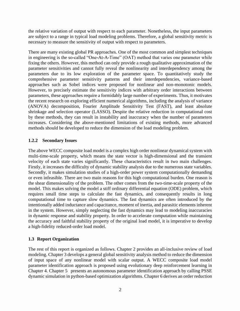
1.2.2 Secondary Issues
The above WECC composite load model is a complex high order nonlinear dynamical system with
multi-time-scale property, which means the state vector is high-dimensional and the transient
velocity of each state varies significantly. These characteristics result in two main challenges.
Firstly, it increases the difficulty of dynamic stability analysis due to the numerous state variables.
Secondly, it makes simulation studies of a high-order power system computationally demanding
or even infeasible. There are two main reasons for this high computational burden. One reason is
the shear dimensionality of the problem. The other comes from the two-time-scale property of the
model. This makes solving the model a stiff ordinary differential equation (ODE) problem, which
requires small time steps to calculate the fast dynamics, and consequently results in long
computational time to capture slow dynamics. The fast dynamics are often introduced by the
intentionally added inductance and capacitance, moment of inertia, and parasitic elements inherent
in the system. However, simply neglecting the fast dynamics may lead to modeling inaccuracies
in dynamic response and stability property. In order to accelerate computation while maintaining
the accuracy and faithful stability property of the original load model, it is imperative to develop
a high-fidelity reduced-order load model.
1.3 Report Organization
The rest of this report is organized as follows. Chapter 2 provides an all-inclusive review of load
modeling. Chapter 3 develops a general global sensitivity analysis method to reduce the dimension
of input space of any nonlinear model with scalar output. A WECC composite load model
parameter identification approach is proposed using evolutionary deep reinforcement learning in
Chapter 4. Chapter 5 presents an autonomous parameter identification approach by calling PSSE
dynamic simulation in python-based optimization algorithms. Chapter 6 derives an order reduction

3
technique based on the singular perturbation theory to obtain a reduced load model. Chapter 7
concludes this report and describes the future research topics.

4
2. Load Modeling Review
2.1 Introduction
Load modeling is essential to power system analysis, planning, and control. For example, studies
have shown the importance of accurate load representations in voltage stability assessment [1].
Although the need for accurate load models is recognized by power system researchers and
engineers [2], more research is imperative to update existing load models and understand
characteristics of modern loads with emerging smart grid technologies such as distributed
generators (DGs), electric vehicles (EVs), and demand side management (DSM). The uncertainty
and difficulty of load modeling comes from the large number of diverse load components, time-
varying and weather-dependent compositions, and the lack of measurements and detailed load
information. The goal of load modeling is to develop simple mathematical models to approximate
load behaviors.
Load modeling consists of two main steps: 1) selecting a load model structure, and 2) identifying
the load model parameters using component or measurement-based approaches. Component-based
or physically-based modeling has been extensively investigated in literature [3]-[9]. The method
is based on the knowledge of physical behaviors of loads and mathematical relations that describe
the functioning of load devices. However, obtaining such information is not always possible,
which motivates the research in measurement-based modeling [10]-[19]. Measurement-based
modeling collects measurements from data acquisition equipment to derive load characteristics.
The main advantage is that this approach directly obtains the data from the actual network, and
can be applied to any load. However, a developed model at one network location may not be
applicable to other locations. The parameters of load models are estimated by fitting the acquired
data to a load model structure using identification and estimation techniques. Other research
suggested the use of Artificial Neural Networks (ANN) to model loads by mapping the input data
set to the output [25]-[30]. This approach is useful when the model structure is unknown or hard
to be mathematically represented. However, data-driven techniques require a large number of
datasets and considerable computational effort. Moreover, ANN-based models can only be applied
to systems for which they were developed.
A review on load modeling was performed in 1990s [31],[32], which included a bibliography [33]
listing papers on load models and typical values of parameters. The International Council on Large
Electric Systems (CIGRE) established a new working group to provide guidance with respect to
load modeling. The working group C4.605: "Modelling and Aggregation of Loads in Flexible
Power Networks" aims to provide an overview of existing load models with a critical analysis on
parameter identification methods. Developing new load models and validation techniques are also
part of the agenda for CIGRE C4.605. The working group conducted a survey on international
industry practice on load modeling in [34]. The paper summarized the key findings from
questionnaires collected from power system operators around the world, and identified the
prevalent types of load models being used. In [35], CIGRE presented a general overview on load
modeling and aggregation. The report included modeling of active distribution networks and a
detailed description of the commercial and residential load sectors. In this paper, we present a
concise and thorough review on load modeling, including DG models. We review the existing
work on load modeling and present the outstanding issues and new research trends. The commonly

5
used load models are summarized and discussed. The ever-increasing integration of demand-side
controls and DGs, particularly distributed PVs, further complicates load characteristics and poses
additional challenges to load modeling. In addition, we introduce the latest advancements in
developing load models, such as the use of real-time data for online modeling [21], modeling
residential loads by considering both electrical characteristics and consumers’ behaviors [36], and
modeling microgrids (MGs) using a combination of component- and measurement-based methods
[37][38].
2.2 Types of Load Models
Load modeling refers to the mathematical representation of the relationship between the power
and voltage in a load bus [2]. Load models can be classified into two main categories: static and
dynamic models. Fig. 2-1 shows the currently used load models in industry for static and dynamic
studies [34].
Fig. 2.1 Load models currently used in the industry for (a) steady-state analysis and dynamic
studies (b) active power and (c) reactive power
2.2.1 Static Load Models
Static models express the active and reactive power at any instant of time as functions of bus
voltage magnitudes and frequency. These models can be used to represent static loads e.g.,
resistive loads, and as an approximation for dynamic loads, e.g., induction motors.
1) ZIP Model
ZIP model is commonly used in both steady-state and dynamic studies [2]. This model represents
the relationship between the voltage magnitude and power in a polynomial equation that combines
constant impedance (Z), current (I), and power (P) components.
2) Exponential Model
The exponential model relates the power and the voltage at a load bus by exponential equations.
This model has fewer parameters and is usually used to represent mixed loads [39]. More

6
components with different exponents can be included in these equations. For example, by using
three exponential components, the exponential model can be converted to a ZIP model.
3) Frequency Dependent Model
This model is derived by multiplying the exponential or ZIP model by a factor that depends on the
bus frequency. The factor can be represented as follows.
( ) 01 ffaFactor f −+= (2.1)
where f is the frequency of the bus voltage, f0 is the nominal frequency, and a, is the frequency
sensitivity parameter. Adding the frequency term to the ZIP model has no physical meaning, since
the component related to the constant impedance becomes dependent on the frequency [32].
4) Electric Power Research Institute (EPRI) LOADSYN Model
This model is used in the EPRI LOADSYN computational program and Extended Transient
Midterm Stability Program (ETMSP) for dynamic studies [40][41]. The model combines ZIP,
exponential, and frequency-dependent models.
( ) ( ) ( )( ) 2
12
1
1 000 /11/ pvpv K
apf
K
aL VVPfKVVPPP −++= (2.2)
( ) ( ) ( )( ) ( )fKVVQPQPfKVVQPQ qf
K
aqf
K
aLqvqv +−++=
2
2
11
1
11//1/ 000000 (2.3)
where P0 and Q0 are the power consumed at the rated voltage V0 of a device, if the model is used
to represent a specific device. If it models the aggregate load at a bus, V0 , P0 and Q0 are initial
operating conditions. The active power is represented by frequency dependent and independent
components. The reactive power is composed of two terms. The first represents the reactive power
consumption of the load, and the second approximates the effect of the reactive consumption minus
compensation, which finds the initial reactive power flow at a bus. Pa1 is the frequency-dependent
fraction of active power, Qa1 is the reactive load coefficient representing the ratio of
uncompensated reactive load to active power, Kpv1 and Kpv2 are voltage exponents for frequency
dependent and independent active power, respectively. Kqv1 and Kqv2 are voltage exponents for the
reactive power without and with compensation, respectively. Kpf1 and Kqf1 are the frequency
sensitivity coefficients for active and uncompensated reactive power load, respectively. Kqf2 is the
frequency sensitivity coefficient for reactive power compensation.
2.2.2 Dynamic Load Models
Studies in voltage stability require the use of dynamic load models for accurate representation [2].
Dynamic models express the active and reactive powers as a function of voltage and time.
Examples of the widely used dynamic models are presented as follows.

7
Fig. 2.2 Schematics of (a) induction motor, (b) ZIP+IM, (c) CLOD, (d) WECC CLM
1) Induction Motor (IM)
In dynamic models, the active and reactive power is represented as a function of the past and
present voltage magnitude and frequency of the load bus. This type of model is commonly derived
from the equivalent circuit of an induction motor [2], shown in Fig. 2.2 (a), where Rs and Rr are
the static and rotor resistances respectively, Xs, Xr and Xm are the static, rotor and magnetizing
reactance, respectively, and s is the rotor slip. The induction motor model is considered as a
physically- based model.
2) Exponential Recovery Load Model (ERL)
The exponential recovery load model [43],[44] represents active and reactive power responses to
step disturbances of the bus voltage. This model is commonly used for representing loads that
slowly recover over a time period, which ranges from several seconds to tens of minutes. ERL is
also used to model on-load tap changers (OLTCs) which restore the nominal supply voltage after
a disturbance. The model is developed as a non-linear first-order equation to represent the load
response, as shown in (4-7).
( ) ( ) ptps NN
p
p
p VVPVVPxdt
dxT 0000 // −+−= (2.4)
where xp and xq are state variables related to active and reactive power dynamics, Tp and Tq are
time constants of the exponential recovery response, Nps and Nqs are exponents related to the
steady-state load response, Npt and Nqt are exponents related to the transient load response.
The ERL is further extended in [45] as an adaptive dynamic model. The model has the same
characteristics as the exponential recovery model, but with the power being a function of the

8
voltage multiplied by the state variable.
( ) ( ) ptps NN
p
p
p VVPVVxdt
dxT 000 // +−= (2.5)
( ) ptN
pd VVxP 0/= (2.6)
( ) ( ) qtqs NN
q
q
q VVQVVxdt
dxT 000 // +−= (2.7)
( ) qtN
pd VVxQ 0/= (2.8)
2.2.3 Composite Load Models (CLM)
Recent studies focus on combining the dynamic and static load models [11],[13],[21],[46][47].
References [46] and [47] compared simulation results of different load models with transient
disturbances, and concluded that composite models can provide more accurate responses. The
widely used composite models are summarized in this subsection.
1) ZIP+IM
According to the study in [34], the composite load model consisting of ZIP and an induction motor
is the most commonly used model in the US industry for dynamic studies. In [13], several
composite load models were considered including ZIP+IM and Exponential+IM. The report
concluded that the ZIP+IM structure is able to model loads with various conditions, locations, and
compositions. The equivalent circuit of the ZIP+IM model is shown in Fig. 2.2 (b).
2) Complex Load Model (CLOD)
This model is adopted by the Siemens PTI PSS/E stability program [31]. CLOD is an aggregate
dynamic model of large and small motors, non-linear models of discharge lighting, transformer
saturation effects, constant MVA, shunt capacitors, and a series impedance and tap ratio to
represent the effect of intervening sub-transmission and distribution elements. Fig. 2.2(c) shows
the schematic of this model.
3) Western Electricity Coordinating Council (WECC) CLM
After the 1996 blackout of the Western Systems Coordinating Council (WSCC) [48], an interim
composite load model containing a static part and a dynamic part was implemented by WSCC
[49]. The model is assumed to have 80% static loads and 20% dynamic ones. The static part is
represented by existing data from WSCC members, and the dynamic part is an induction motor
model. The model was designed to capture the effects of dynamic induction motor loads for highly
stressed conditions in summer peaks. The interim load model was unable to represent delayed
voltage recovery events from transmission faults [5][50],[51]. WECC improved the interim model
[6] by adding the electrical distance between the transmission system and the electrical end-uses,

9
as well as adding special models for residential air- conditioners. By 2012, the WECC CLM was
tested and implemented in major industry-level simulation software including PowerWorld
Simulator and Siemens PTI PSSE [6]. Datasets were developed for four seasons in 12 climatic
zones across the western region with different load sectors (residential, commercial, mixed and
rural)[6]. The model structure is shown in Fig. 2.2 (d), which includes an electrical representation
of a distribution system with a substation transformer, shunt reactance, and a feeder equivalent. At
the consumer side, the load model includes a static load model, one power electronics model, and
four types of motor models. Although CLM provides a detailed modeling, it is hard to implement
as there are 131 parameters to be identified.
2.2.4 Artificial Neural Network-Based Modeling
ANN-based load modeling [25]-[30] matches observed system behaviors without using a physical
form to obtain the output, i.e., it has no physical meaning and purely relies on measurement data.
An ANN is composed by a set of processing units interconnected by weights. The ANNs are
trained using a succession of input and output patterns, resulting in the final values of the
connection weights that determine the load model. Reference [25] presented two ANN-based load
modeling approaches. In [26], an ANN-based composite load model was proposed for stability
studies. The authors used a two-step procedure with the first step to develop a recurrent neural
network with simulation data and the second step to update it using measurement data. Although
ANN is powerful in representing complex nonlinear systems., obtaining enough data over a wide
range of operation conditions is challenging. In addition, ANN-based models must be updated
periodically when new measurement datasets are available.
2.3 Load Model Parameter Identification
Load model identification methods can be classified into two categories: component-based and
measurement-based. The component-based methods aggregate models of individual electrical
components to form an aggregated load model. This approach requires knowledge on the load
composition, i.e., the percentage of load consumed by each type of load components.
Measurement-based approaches leverage data from devices such as PMUs, smart meters, etc. A
model structure is selected and its parameters are derived using computation techniques such as
statistics, artificial intelligence, and pattern recognition. Component-based methods start from the
individual components, while measurement-based ones start from the measurement data as
illustrated in Fig. 2.3. The two methods are summarized in Table I.

10
Fig. 2.3 (a) component-based modeling approach, (b) measurements-based method approach
2.3.1 Component-Based Approach
The component-based method is a bottom-up approach as illustrated in Fig. 8 (a). Load is
commonly divided into industrial, commercial, and residential classes. The approach requires three
datasets: 1) models of individual components, 2) component composition, i.e., the percentage of
load consumed by each load component, and 3) class composition, i.e., the percentage contribution
of each load class to the aggregate load. This approach has been used by WECC to develop their
composite load models [6].
The individual load components can be represented using static or dynamic models. Resistive
components such as electric cooking appliances and water heaters can be modelled as constant-
impedance loads, while other loads such as SMPS are modeled as constant-power loads or the
generic model in Fig. 2.3 [36]. The parameters for individual component models can be obtained
through laboratory experiments [52]-[54].

11
Table 2.1 Comparison of measurement and component based approaches
Determining the load composition is the most challenging task as it is impossible to obtain detailed
consumption information of all electrical components in a power system. In addition, load
composition is affected by geographical locations and weather conditions. For example, Fig. 2.4
show consumption profiles of different appliances in residential and commercial sectors during
different seasons. Recently, the deployment of smart meters enables the two-way communication
between customers and utilities, which provides a new and easy way to obtain accurate load
compositions. To determine the load class composition, the metered demand at load buses can be
used, which is typically available every 15 minutes.
Fig. 2.4 Typical consumption profiles for (a) winter commercial class, (b) winter residential
class, (c) summer commercial class, and (d) summer residential class
Advantages Disadvantages
Mea
sure
men
t-bas
ed
- Based on data from actual systems
- Provide accurate models for
measured locations and time
- A generic method that can be applied
to various models
- No need to have deep
knowledge of loads
- Unable to account for different
operation conditions
- Models are developed using data
measured in certain periods at specific
locations, which lacks generalizability
- Measurements with large
disturbances are hard to obtain
Com
ponen
t-bas
ed - Field measurement is not required
- Physical representation of end-use
devices
- Can be applied to different operation
conditions
- Demand side management is
considered
- Requires characteristics of individual
load components.
- Accurate and comprehensive load
composition information is hard to
obtain
- Low adaptability to the integration
of new loads

12
A different bottom-up approach was proposed in [55] for industrial facilities. Instead of obtaining
the full load model of the system by using composition values of load classes, the paper proposed
to create specific models for industrial loads, then obtain the system model using an aggregation
algorithm developed in [56].
2.3.2 Measurement-Based Approach
Steps of the measurement-based approach are summarized in Fig. 2.3 (b): 1) obtain measurement
data, 2) select a load model structure (e.g. ZIP, exponential, etc), 3) estimate model parameters,
and 4) validate the load model. Measurement-based
load modeling leverages actual field data to capture load characteristics. The measurements should
be obtained under different conditions and disturbances. The model parameters are estimated by
minimizing the difference between the response of the load model and the field measurements.
The problem can be formulated as a curve fitting problem using the following equation:
( ) ( ) =
−+−n
i
e
i
m
i
e
i
m
i QQPPn 1
221min (2.9)
where Pim and Qi
m are the measured active and reactive power, respectively, and Pie and Pi
e are the
modeled active and reactive power, respectively. The parameters are calculated using algorithms
such as least-squares, genetic algorithm (GA), support vector machines (SVM), Kalman Filter
(KF), Levenberg-Marquardt algorithm, and Simulated Annealing. Table II summarizes existing
measurement-based techniques.

13
Table 2.2 Examples of measurement-based techniques
The measurement-based approach has been extensively studied in the literature. In [11], a
multicurve identification technique was used to identify parameters of the ZIP+IM model. Multiple
filed measurement datasets were collected and fitted to the model structure using a hybrid GA and
simplex search algorithm. [21] presented an event-oriented method for online load modeling based
on PMU data from the Illinois Institute of Technology MG. In [22], the authors used the sliding
window technique to reflect the real-time dynamic behaviors of loads during disturbances such as
voltage sags and interruptions. Least-square methods have been widely applied to identify
parameters of various load models including ZIP+IM with frequency. The increasing installation
of PMUs makes the online modeling an attractive approach. Reference [66] applied the unscented
Kalman filter [67] to perform real- time estimation of the ERL model parameters. The developed
approach was tested on both simulated and field measurements with a 3-second resolution. In [65],
a time-varying exponential load model was used to represent the load, and a recursive least square
Ref. Algorithms Load Models Data Sources
[17] GA + Simplex search
method ZIP+IM PMU: NE power grid in
China
[20] GA+LM ZIP+IM Simulation + Field
measurements
[22] Improved particle swarm
optimization Exponential + IM
Simulation + Laboratory
experiments
[42] LM ERL Simulation + Field
measurements
[57] Least Square 1st order IM model Simulation
[58] Gauss-Newton +
Trajectory sensitivity Differential- algebraic
equations Simulation
[59] Instrumental Variable-
based estimation
ZIP and Exponential and
dynamic models Simulation
[60] Gradient-based
parameter estimation Fifth-order single rotor cage
model Laboratory experiments
[61] Simulated Annealing EPRI Loadsyn and IM Simulation + Field
measurements
[62] Kalman Filter ZIP Korea Energy
Management System
[63] SVM ZIP+IM Simulation
[64] Weighted recursive least
squares Exponential and ZIP CPFL Energia, Brazil
[65] Recursive least squares Exponential Field CVR test data

14
algorithm was employed to identify the load model parameters. The paper used the load model to
assess conservation voltage reduction (CVR) effects [68]. The authors in [69] used robust least
squares approach to estimate time-varying parameters of a ZIP model at the substation level. The
proposed method was used to identify the load-to-voltage dependence and analyze CVR.
There are studies using hybrid component- and measurement-based methods. [70] developed load
models at high-voltage buses from load compositions of LV buses. SVM was used to classify the
loads into various classes based on the load responses to large disturbances. The authors in [71]
proposed a variable projection based optimization algorithm to identify the parameters of several
different load models. For small disturbances, only the load component composition in each load
class was identified, and the remaining parameters remained unchanged. The proposed method
was tested on the 243-bus Indian Northern Regional Power Grid system. Reference [72] developed
an approach to aggregate various load component models to obtain the system load model.
Parameter estimation was used to determine the amount each component contributes to the total
power consumption. A Gauss-Newton method based on trajectory sensitivities was used to
determine the parameters of each load model structure. Trajectory sensitivities can quantify effects
of small parameter changes on a dynamic system’s trajectory, which can guide the parameter
updates.
The authors in [14] used trajectory sensitivity for model simplification to reduce the number of
parameters to be estimated. By applying the trajectory sensitivity analysis to measurement data,
load model parameters were classified into two sets based on their sensitivities to the active and
reactive power. Parameters with large sensitivities were grouped together and estimated using the
measurement-based approach, while less sensitive parameters were set to be their default values.
The parameters with low sensitivities are not necessarily unimportant, it means these parameters
are hard to be identified from the current data. Reducing the number of parameters makes it
possible to include more components in the load model. [23] presented an algorithm for estimating
load model parameters based on the analytical similarity of model parameter sensitivities, and
demonstrated its computational efficiency and accuracy. The authors in [73] analyzed model
parameter sensitivities using eigenvalues of Hessian matrix. The paper used the LM algorithm to
solve the optimization problem. The linear dependence between two load model parameters were
then identified by examining the condition number of Jacobian matrix. This dependency analysis
was used to ensure that low-sensitivity parameters were independent of high-sensitivity ones.
Reference [74] presented a computationally efficient technique for estimating the composite load
model (ZIP+IM) parameters based on analytical similarity of parameter sensitivity. The paper used
the partial derivative of each parameter to identify parameters with similar sensitivities. LM
algorithm was used to solve the optimization problem in (17). The presented technique was tested
on real measurements collected from Cheongju and Suwon of South Korea. The computation time
was reduced by three quarters after reducing the number of parameters from 12 to 9.
2.4 Summary
This section reviews the state-of-the-art of load models and parameter identification methods. New
approaches for modeling LV networks and ADNs are also discussed. Load modeling is challenging
due to the large number of diverse load components, the lack of precise load composition
information, and the stochastic, time-varying and weather-dependent load behaviors. Currently,
the ZIP+IM composite model is one of the most widely used models in US power industry [34].

15
WECC and EPRI have been actively investigating load modeling techniques. WECC focused on
the component-based approach while EPRI is developing hybrid approaches that integrate
component- and measurement-based methods. The WECC composite load model is
comprehensive and flexible, however, it is complicated and hard to apply. There are also concerns
about the numerical stability and consistency of the WECC model. ZIP+IM is less complicated,
but it is unable to capture the full system characteristics. Furthermore, ZIP+IM cannot represent
DGs’ behaviors. CIGRE provided several overviews and recommendations on load modeling
which were combined in [75][77].
For parameter identification, measurement-based techniques are prevalent as new devices such as
PMUs and smart meters are installed. However, it is still challenging to identify a large number of
unknown parameters. Sensitivity analysis has been proposed to reduce the number of parameters
and identify the significant ones. Extreme sensitivities could lead to the failure of the load model
with small changes in operating conditions. Further research on sensitivity analysis is needed. The
deployment of smart measurement devices provides an opportunity to design hybrid approaches
that integrate the measurement- and component-based methods. The introduction of new loads and
controls will reshape the load composition. The deployment of smart meters provides an
opportunity to improve the load composition estimation for component-based load modeling [78].
The amount of data collected from the measurement devices is massive, and processing a large
number of data is challenging. Data collection and processing techniques such as data mining and
clustering should be improved. Future research on parameter estimation algorithms should be able
to process data from existing and emerging measurement devices with different resolutions, such
as smart meters, PMUs, and SCADA. Meanwhile, the algorithms should be robust to bad data,
missing measurements, changes in the voltage regulation scheme, and noises [79]-[80].

16
3. Parameter Reduction of Composite Load Model using Active Subspace
3.1 Introduction
Load modeling is significant for power system studies such as parameter identification,
optimization and stability analysis, which has been widely studied [81]. It can be classified into
static and dynamic load models. Constant impedance-current-power (ZIP) model, exponential
model and frequency dependent model are typical static loads models, and traditional dynamic
load models include induction motor (IM) and exponential recovery load model [82]. To provide
more accurate responses, composite load models are developed by combining static and dynamic
load models. Motivated by the 1996 blackout reported by the Western Systems Coordinating
Council (WSCC), the classic ZIP+IM composite load model was developed to model highly
stressed loading conditions in summer peak hours [83]. However, this interim load model was
unable to capture the fault-induced delayed voltage recovery (FIDVR) events [84]. Therefore, a
more comprehensive composite load model was proposed by Western Electricity Coordinating
Council (WECC) that contains substation trans-former, shunt reactance, feeder equivalent,
induction motors, single-phase AC motor, ZIP load, electronic load, and DER [85]. WECC
composite load model (WECC CMLD) produces accurate responses, nevertheless, the large
number of parameters and high model complexity raise new challenges for power system studies.
Name parameter identification as one significant example, where the large number of parameters
brings great difficulties to search for global optimum when performing parameter identification.
The reason is twofold: firstly, the large number of parameters result in a large search space that
reduces the optimization efficiency; secondly, the insensitive parameters and parameter
interdependencies usually result in a large number of local optima, which increases the difficulty
of achieving global optimum [86]. Although the parameters have physical meanings, some of them
only have marginal impacts on the model response altogether or along certain parameter variation
directions [87]. Moreover, considering full load model parameter set could significantly increase
the complexity of power system studies. Therefore, it is imperative to develop a method to screen
out the insensitive parameters. Then, only the sensitive parameters are to be determined in the
parameter identification problem while the others can be kept at their respective default values. In
this way, the dimension of search space of load model parameters can be significantly reduced.
Thus, lower computational cost (less model runs) and higher accuracy (easier to find the optimum)
can be achieved when conducting power system studies such as parameter identification without
compromising fidelity of the load model.
The above problem can be resolved by dimension reduction in parameter space based on sensitivity
analysis of a parameterized model whose inputs are system parameters. As discussed in [88],
parameter reduction (PR) methods can be classified into local and global ones. Local PR methods
are suitable for known parameters with small uncertainties, in which partial derivatives of output
with respect to the model parameters are computed to evaluate the relative variation of output with
respect to each parameter. Nonetheless, the input parameters are subject to a range in typical load
modeling problems. Therefore, a global sensitivity metric is necessary to measure the sensitivity
of output with respect to parameters.
There are many existing global PR approaches. One of the most common and simplest techniques
in engineering is the so-called “One-At-A-Time” (OAT) method that varies one parameter while

17
fixing the others. However, this method can only provide a rough qualitative approximation of the
parameter sensitivities and cannot fully reveal the nonlinearity and interdependency among the
parameters due to its low exploration of the parameter space. In [89], the OAT method was
improved by proposing two sensitivity measures, mean µ and standard deviation σ based on the
elementary effects methods. This method has higher exploration rate of the parameter space and
can qualitatively analyze which parameter may have influence on nonlinear and/or interaction
effects. This method is further extended by supersaturated design [90], screening by groups [91],
sequential bifurcation method [92] and factorial fractional design [93] based on the number of
parameters and experiments in a particular scenario [94].
To quantitatively study the comprehensive parameter sensitivity patterns and their
interdependencies, variance-based approaches such as Sobel indices [95] were proposed for
nonlinear and non-monotonic models. However, to precisely estimate the sensitivity indices with
arbitrary order interactions between parameters, these approaches require a formidably large
number of experiments [96]. In [97], a total-effect index was introduced, which can measure the
contribution to the out-put variance of parameters, including all variance caused by its interactions
of any order with any other parameters, as well as reducing the requirement of the number of
experiments. These indices are usually estimated by Monte Carlo methods [98]. Such methods are
accurate but suffer from high computational cost when large sample size is required. Thus, it
motivates the recent research on exploring efficient numerical algorithms including the analysis of
variance (ANOVA) decomposition [99], Fourier Amplitude Sensitivity Test (FAST) [100] and
least ab-solute shrinkage and selection operator (LASSO) [101]. Despite the relative reduction in
computational cost by these methods, they can result in instability and inaccuracy when the number
of parameters increases (larger than 10) [94], [102]. Some researches delve into the trajectory
sensitivity analysis, e.g., in [103], the time-varying parameter sensitivities of ZIP+IM model are
derived based on perturbation and Taylor expansion method. However, such methods need explicit
mathematical model and require the model output to be differentiable with respect to the
parameters for the Jacobian matrices to exist, which makes it inapplicable for WECC CMLD.
Different from OAT and and variance-based approaches, the active subspace method (ASM) is
based on gradient evaluations for detecting and exploiting the most influential direction in the
parameter space of a given model to construct an approximation on a low-dimensional subspace
of the model’s parameters as well as quantify the interdependencies among parameters [104]. As
a Monte Carlo sampling based method, ASM also requires multiple experiments, but it has better
accuracy and requires relatively lower sample size.
There are limited studies on the PR problem of WECC CMLD. In [81], the parameter sensitivity
and interdependencies among parameters are analyzed using OAT method and clustering
techniques, motivated by observing that different parameter combinations can give the same data
fitting results in measurement-based load modeling. As discussed above, the OAT method suffers
from low accuracy and low exploration rate of the parameter space. Moreover, the interdependency
is simply determined by whether parameters have similar trajectory sensitivities in this work. In
addition, the newly-approved aggregated distributed energy resources (DER A) model in WECC
CMLD has not been considered. PR was conducted by means of data-driven feature-wise
kernelized LASSO (FWKL) in [101], which uses multiple randomly-generated parameter vectors
and corresponding output residuals to compute parameter sensitivities by solving a LASSO
optimization problem. This approach avoids utilizing analytical gradient and can obtain the
optimal sensitivity. In addition, the employment of LASSO ensures parameter interdependency is

18
captured in a feature-wise manner. However, due to high non-convexity of WECC CMLD, the
result is very sensitive to parameter setting of the algorithm and the distribution of the dataset.
Also, the large number of experiments and optimization process greatly increase its computational
cost.
In this chapter, a novel PR approach is proposed by leveraging the ASM. As an alternative PR
technique, ASM is a relatively new dimension reduction tool that has shown its effectiveness in
many fields such as bioengineering [105] and aerospace engineering [106]. The outstanding
advantages of ASM include relatively low computational cost, high accuracy and the ability to
quantify the parameter interdependency.
Motivated by the fact that the WECC CMLD is a differential-algebraic system and ASM can only
deal with algebraic functions, we first cast the WECC CMLD as a discrete-time system for
parameterization. Secondly, a comprehensive PR approach tailored for WECC CMLD based on
ASM is proposed. Thirdly, factors influencing accuracy of PR results are rigorously analyzed.
Finally, statistical and numerical experiments are conducted to validate the effectiveness of the
proposed method. Comparative case studies with three classical PR methods are also conducted
and discussed.
3.2 Problem Statement
In this section, the structure and function of WECC CMLD are introduced, then a parameterized
model of the composite load is established for PR.
3.2.1 Introduction of WECC CMLD
As shown in Fig. 3.1, WECC CMLD consists of three 3-phase motors, one single-phase motor,
one ZIP load, one electronic load and one DER A model. Three 3-phase motors represent three
different types of dynamic components. Motor A represents three-phase induction motors with
low inertia driving constant torque loads, e.g. air conditioning compressor motors and positive
displacement pumps. Motor B represents three-phase induction motors with high inertia driving
variable torque loads such as commercial ventilation fans and air handling systems. Motor C
represents three-phase induction motors with low inertia driving variable torque loads such as the
common centrifugal pumps. Single-phase motor D captures behaviors of single-phase air with
reciprocating compressors. However, it is challenging to model the fault point-on-wave and
voltage ramping effects [85]. Moreover, new A/C motors are mostly equipped with scroll
compressors and/or power electronic drives, making their dynamic characteristics significantly
different than conventional motors. Therefore, WECC uses a performance-based model to
represent single-phase motors. As increasing percentage of end-uses become electronically
connected [83], the WECC CMLD adopts a simplistic representation of power electronic loads as
constant power loads with unity power factor. A ZIP load is used as static one in this model. The
DER model is specified as the newly-approved DER A model presented in [107].

19
Fig. 3.1 A schematic diagram of the WECC CMLD[108]
3.2.2 Motivation for PR
The WECC CMLD contains 183 parameters, which pose significant challenges for power system
studies such as parameter identification, optimization and control. By observing that part of the
parameters can be determined by engineering judgment, we can filter out them according to the
analysis in [101]. In particular, the parameters of transformer, feeder, and the stalling and restarting
of induction motors can be excluded since they have small range of uncertainties and are usually
pre-determined by their default values to meet practical engineering requirements. In this way, 64
parameters are screened out a priori. Nonetheless, the number of parameters that remains is still
too large for power system studies. Therefore, in this chapter, we use ASM to further reduce the
number of parameters. The WECC CMLD is a differential-algebraic system which is usually
represented as a continuous-time state space model [84]. Considering that ASM requires a scalar
function with domain as parameters and range as active or reactive power, in this section, we
parameterize the WECC CMLD in a discretization manner. The parameterized model produces
similar responses as the original one with high-fidelity as long as the Nyquist-Shannon sampling
theorem is satisfied.
3.2.3 Parameterized WECC CMLD
The WECC CMLD is a hybrid model with dynamic and static components. The state vector dn
x ¡ of three-phase motors and DER is governed by the following differential equation
( ) ( ) ( ) ( )( ), , , x t f x t t u t=& (3.1)
where ( ) pnt ¡ denotes the parameter vector; ( ) ( ) ( ) ( ) , ,
T
u t V t t f t = is the input
vector consisting of volt-age magnitude, voltage angle and frequency deviation, respectively; 3: pd d
nn nf →¡ ¡ ¡ ¡ represents the dynamic model of three-phase motors, and DER; dn and
pn are the total number of dynamic states and parameters. The active and reactive power output
of the dynamic components, ( ) ( ) ( ),T
d d dy t P t Q t= is given by

20
( ) ( ) ( ) ( )( ). , , d dy t g x t t u t= (3.2)
In PR using ASM, a mapping between parameters and active/reactive power is required for PR.
Based on the fact that the input of load model u is usually sampled every T seconds, we can
discretize (3.1) as
( ) ( ) ( ) ( )( ) 1 , 1 , , 1x k f x k k u k= − − − (3.3)
where f is the discretized function of f, k = 1, 2, . . . , N, N is the total number of measurements.
Note that the sampling rate should satisfy Nyquist-Shannon sampling theorem to guarantee that
discrete sequence of samples can capture all the information from a continuous-time signal. Then,
( )x k can be calculated from the initial state ( )0x by iteratively evaluating f using past
sequences of parameters and inputs, ( ) ( ) ( ) ( )1 , . . . , 0 , 1 , . . . , 0k u k u − − . Finally, by
substituting (3.3) iteratively into (3.2), we can obtain the desired mapping using some algebraic
function dg :
( ) ( ) ( ) ( ) ( ) ( )( ) , . . . , 0 ., , . . . , 0 , 0d dy k g k u k u x = (3.4)
Regarding x and u as constants, Eq. (3.4) depicts the relation-ship between active/reactive power
of dynamic components and parameters.
As for the static components such as single-phase motor, electronic load, and static ZIP load, the
mapping from parameters to active and reactive power outputs can be represented as
( ) ( ) ( )( ) , .s sy k g k u k= (3.5)
The total power output ( )y k of the WECC CMLD can be calculated by adding the dynamic and
static parameterized model together. For ease of deriving PR approach for the composite load
model, we define the parameterized model as g in the form of
( ) ( ) ( ) ( ) ( ) ( ) ( ) ( )( ) , , 0 , , , 0 , 0 . d sy k y k y k g k u k u x = + = K K (3.6)
If the parameters are considered as time-invariant during a short time period, Eq. (3.6) can be
simplified as
( ) ( ) ( ) ( )( ) , , . .. . , 0 , 0y k g u k u x= (3.7)
where ( ) ( ) ( ),T
y t P t Q t= , and ,T
P Qg g g = .

21
3.3 PR Approach for WECC CMLD using ASM
In this section, we will use ASM to reduce the parameters of the WECC CMLD. Firstly, the
preliminaries of ASM are introduced. Then, the application of ASM to WECC CMLD is
elaborated in steps. Finally, the factors affecting the accuracy of PR is analyzed theoretically.
3.3.1 Preliminaries of ASM
An active subspace is a lower-dimensional linear subspace of the parameter space, along which
input perturbations alter the model’s predictions more than the perturbations along the directions
which are orthogonal to the subspace on average. This subspace allows for a global measurement
of sensitivity of output variables with respect to parameters, and is often used to decrease the
dimension of the parameter space. Con-sider a parameterized function :g → ¡ that maps the
parameters of a system, : | 1 1, 1, ,m
ix x i m = − =¡ K , to a scalar output of interest,
e.g., active power P or reactive power Q, where indicates a normalized set of parameter values.
To discover the active subspace, we define the following C matrix,
( )( ) ( )( ) ( ) . T
g gC d
= (3.8)
where ( ) : +→ ¡ is the joint probability function of parameters satisfying
( ) 1.d = (3.9)
For any smooth function ( )g , the matrix C is called average derivative functional in the context
of dimension reduction, which weights input values according to the density ( ) . Note that a
single normalized parameter is a random variable taking values in [−1, 1], which when
appropriately scaled represents a parameter in the original model (3.7). Since the dimension of the
parameter space in this model is 64, we take m = 64 throughout. The matrix C is the average of the
outer product of the gradient of ( )g with itself and has some useful properties that will allow us
to deduce information about how ( )g is altered by perturbations in its arguments.
Remark 1: From (3.8), each element of C is the average of the product of partial derivatives (which
can be regarded as parameter sensitivity)
, , 1, , ,ij
i j
Cg g
d i j m
= = K (3.10)
where ijC is the (i, j) element of C, and m is the number of parameters. If we consider ( )g
to be a random vector by virtue of 'i s density ρ, then C is the uncentered covariance matrix of

22
the gradient of output with respect to the parameters [104]. This allows us to use the covariance
matrix C to measure the correlation between each pair of parameter gradients. For simplicity,
denote i
g
as is , denote the mean and standard
deviation of gradient of ith parameter as is and
is , respectively. Then, the correlation between
(i, j) parameter gradients is
( )( )
,
cov( , )
i j
i j
i j
i j
i j
i j
i j
s s
s s
i s j s
s s
ij s s
s s
s s
s s
C
=
− − =
−=
(3.11)
Eq. (3.11) shows that the C matrix encodes the correlation information between parameter
gradients, which means the ASM takes into consideration the interdependency of parameters. This
is one of the advantages compared to other PR methods.
The matrix C is symmetric, and thus permitting the spectral eigen-decomposition
TC W W= (3.12)
where W is an orthogonal matrix whose columns ( ), 1, ,i i m = K are the orthonormal eigenvectors
of C. ( )1, , mdiag = K , and 1 , , m K .
Since W is orthogonal, from the definition of eigenvectors and (3.8), the eigenvalues of C can be
calculated as
( )( ) ( )( ) ( )
( )( )( ) ( )2
, 1, ,
T
i i i
TT
i i
T
i
C
g g d
g d i m
=
=
= =
K
(3.13)
From (3.13) we see that the eigenvalues of the C matrix are the mean squared directional
derivatives of ( )g in the direction of the corresponding eigenvector. If an eigenvalue is small,
then (3.13) shows that ( )g is insensitive in the direction of the corresponding eigenvector on
average. On the contrary, a large eigenvalue indicates that ( )g changes significantly in the
direction of the corresponding eigenvector.

23
After determining the eigen-decomposition (3.12), the eigen-values and eigenvectors can be
separated according to the magnitudes of eigenvalues:
1 1
2 2
0 0,
0 0
WW
W
= =
(3.14)
where 1 and 1W contain the first n larger eigenvalues and corresponding eigenvectors, 2 and
2W contain the other m− n smaller ones. To determine such separation, one can find the spectral
gap between the nth and (n+1) th eigenvalues on a log plot in the order of magnitudes. It is worth
noting that the existence of a significant spectral gap directly indicates the existence of active
subspace [24].
Keeping in mind that W is orthogonal, from (3.14), any parameter vector can be represented as
1 1 2 2
1 1 2 2
T
T T
WW
WW W W
W W
=
= +
= +
(3.15)
Then, an output of interest with any parameter vector is
( ) ( )1 1 2 2g Wg W = + (3.16)
From the definition of 1W and 2W , we know that small perturbations on 2 have low impact on
the value of g. Conversely, small perturbations on 1 will alter g significantly. According to this
property, the range of 1W is defined as the active subspace, and on the contrary, the range of 2W
as the corresponding inactive subspace of the model. These subspaces describe the sensitivity of
the output of interest with respect to parameter variations.
It is worth noting that, though both ASM and principal components analysis (PCA) include the
process of eigen-decomposition, they are intrinsically different. The PCA eigen-decomposed the
covariance matrix of the parameter vector , whereas the matrix to be eigen-decomposed in the
active subspace is defined as (3.8).

24
3.3.2 PR Algorithm Based on ASM
The overall algorithm for PR of WECC CMLD using ASM is summarized in Fig. 3.2. The key
idea of the algorithm is elaborated in details as follows:
Fig. 3.2 The block diagram of the proposed PR algorithm based on ASM
Step 1: Construct the parameter set 1,1m
= − , m = 64 as the normalized parameter space for all
the selected parameters of WECC CMLD, and draw M samples , 1, ,j j M = K from
according to some probability density function satisfying (3.9). Usually, uniform distribution is
chosen for simplicity.
Step 2: For each sampled parameter vector j , approximate the gradient ( )j jg g
= using
first order forward finite differences method as follows:
( ) ( )
( ) ( ),
,1 ,1 ,
,,
,
1
1
1
, ,
,
, 1, , ,( )
j j j
j
j m j m j m
j m
j
j
j m
gg
g
g
j M
g g g
+ − = = + −
M M K (3.17)
where j is an arbitrarily small positive vector perturbation from the sampled parameter values.
When g is a practical system, e.g., WECC CMLD, one needs to transform the normalized
parameter vector j to j that is in the standard range of parameters, using the following linear
mapping,
( ) ( )( )1
.2
j upper lower j upper lowerdiag = − + − (3.18)
where upper and lower are upper and lower bounds of the parameter vectors, respectively. Thus,
j in (3.18) denotes the vector of real parameter values of the WECC CMLD.

25
Step 3: Approximate the average derivative functional C using Monte Carlo simulation as
( )( )1
1ˆ .M
T
j
j jC C gM
g
=
= (3.19)
Step 4: Compute the eigen-decomposition of approximate matrix C :
'ˆ ˆ ˆ ˆ ,TC W W (3.20)
which is equivalent to calculating the singular value decom-position of the matrix
1
1 ˆ ˆ ˆ ,, , T
M Wg g VM
= K (3.21)
where the singular values are the square roots of the eigen-values of C and the left singular vectors
are the eigenvectors of C . The singular value decomposition perspective was first used in
[109][29] to determine the active subspace that is related to the principal components of a
collection of gradients.
Step 5: After the decomposition (3.21), one needs to search for the largest spectral gap among
eigenvalues in for subspace separation. The existence of a larger spectral gap indicates a more
accurate determination of active subspace. To automatically find the optimal separation, we can
use the following equation,
1
1
ˆ ˆˆ , 1, , 1,
ˆi i
i i m
+− = = −K (3.22)
Then, the dimension of the active subspace is
( )( )11, , 1
ˆdim arg max ii m
range W = −
= K
(3.23)
From (3.23), we know that the index of the largest value of ˆi indicates the location of the largest
spectral gap. In the dimension reduction context, often only the first value 1 is considered such
that the dimension of the active subspace is limited to one, which makes it more convenient for
visualization of the output as a function of the active subspace [104][24]. Then, the magnitudes of
elements in the first eigenvector describe the weights of parameters.
Remark 1: The active subspace describes the most sensitive direction in the parameter space along
which the output of interest evolves fastest. Thus, from (16) the output of parameterized model
can be approximated by only the active subspace of parameter space, i.e.,
1 1 1 1( ) ( ), .Tg g W W = (3.24)

26
Eq. (3.24) indicates that g is related to 1 which is a linear combination of original parameters .
This linear combination reflects the weight of each parameter and their collective influence on the
output of interest.
The accuracy of the approximation (3.24) depends mainly on two factors which will be further
discussed in the next subsection.
3.3.3 Accuracy Analysis of PR Based on ASM
In this subsection, two main factors affecting the accuracy of PR using ASM introduced above
will be discussed.
1)Sample size M: In the above algorithm, the most costly computation processes are eigen-
decomposition and computing gradient for M times. In our case, the number of parameters is m =
64, so the computational cost of eigen-decomposition is negligible compared to the computation
of gradient. Thus, the selection of M that is large enough for approximating and W while
minimizing the computational cost is of vital importance. To estimate the first n eigenvalues of
matrix C, the sample size M can be chosen as
( )log ,M n m= (3.25)
where β is an oversampling factor, which is usually selected between 70 and 120. In the next
section, we will verify that this range of β is sufficient in the PR of WECC CMLD by experiment.
The logarithm term log(m) follows from the bounds in the theorem proposed in [109].
2)Gradient approximation: The WECC CMLD suffers from high nonlinearity and complexity that
render it difficult to derive a closed-form expression of gradient of output of interest with respect
to the parameters. In view of the simulating g is not too expensive nor too noisy and m is not too
large, we can utilize finite difference method to estimate the gradient. We know that, a smaller δ
produces a more accurate approximation but with increased computational cost and vice versa.
This relationship can be expressed as the following inequality by using (3.17),
( ) ( )( ) , 1, , ,( )
j j j
j j
j
m jg g
g M
+ − =− K (3.26)
where ( )0
lim 0j
j
→
= .
In the following, we will give a criterion for the selection of finite difference perturbation j by
restating Theorem 3.13 from [104].
Theorem 1 (Accuracy criterion of estimated active subspace [Thm. 3.13 in [104]]): Assume that
( )jg L
for 1, . . . , ,j M= and choose small parameter ε and β in (25) satisfying

27
1
1
0 ,5
n n
+−
(3.27)
2
1
2 2
1
1max , .
n
L
n
(3.28)
If the finite difference perturbation is small enough such that
( ) ( )2
' ' 1ˆ ˆ5 10 , 1, , ,j j n nm L m j M ++ − = K (3.29)
then, the distance between real active subspace 1W and the approximated one 1W using Monte
Carlo and finite difference approximation method is bounded by
( ) ( )( )( ) ( )
( ) ( )
2
1 1
1
1
1
4 8ˆ ,
1 1
4
j j
n n
n n
m L mdist range W range W
+
+
+
− − +
+−
(3.30)
for 1, , ,j M= K with high probability.
Proof: The proof follows the similar steps as in [104] by simply combining (3.25) and (3.28).
We choose 61 10j−= , L = 1, m = 64, ε = 0.1, β = 100 and ( )j j = such that (3.27)-(3.29)
hold. Then, based on Theorem 1, the error of active subspace estimate is bounded by 0.8 and the
simulation result is not too far off.
Remark 2: When the two factors are appropriately set, another most influential factor is the
normalized eigenvalue separation 1 1/ n n +− in (3.30), which depends on the system
characteristics only. The existence of significant spectral gap indicates a clear active subspace and
accurate estimation.
3.4 Case studies
In this section, the proposed ASM is applied to analyze the sensitivities of the parameters of WECC
CMLD. Firstly, a basic case study is conducted to show the implementation process and how to
interpret the result. Then, the proposed method is also applied to the FIVDR case to show its
effectiveness on more complicated voltage profile. Finally, three classical PR techniques are
applied to the WECC CMLD for comparison with the proposed method.

28
3.4.1 Case I: Apply ASM to WECC CMLD and Result Analyses
1)Simulation Setup: We first provide the simulation setup for the case studies. The range of
parameters ,upper lower is set by adding plus and minus fifty percent of perturbations on the
standard values given in the guideline of WECC CMLD [108] as shown in Table 3.1. Using (3.25)
with m = 64, n = 1 and β = 120, the sample size is calculated as 500ASMM . In Section 3.4.3, we
will show the convergence of parameter sensitivity with respect to increasing sample size, from
which we can conclude that 500ASMM = is a good balance between accuracy and computational
cost. Then, the samples are drawn uniformly from . When approximating the gradient using
(3.17), the finite difference perturbation δ is chosen as 61 10− , which is small enough to satisfy
(3.29). Since ASM assumes scalar function g, we conduct the simulation by selecting active and
reactive power as output of interest separately. The voltage and power measurements for PR in
this simulation is generated by the Power System Simulator for Engineering (PSS/E) and the
ACTIVSg500 test case with a line-to-ground fault [101] as shown in Fig. 3.3. The case study is
conducted on a standard PC with an Intel(R) Xeon(R) CPU running at 3.70 GHz and with 32.0
GB of RAM using MATLAB.
Fig. 3.3 The load bus inputs: (a) voltage magnitude; (b) voltage angle; (c) frequency

29
Table 3.1 Numerical range of load parameters of WECC CMLD
Parameter LB UB Parameter LB UB Parameter LB UB
Motor A LppC 0.06 0.24 Electronic Load
TpoA 0.046 0.184 LsC 0.9 3.6 Frcel 0 0.38
TppoA 0.001 0.004 RsC 0.015 0.06 Vd1 0.5 1.5
LpA 0.05 0.20 HC 0.1 0.4 Vd2 0.25 1
LppA 0.042 0.168 EtrqC 1.8 2.2 DER_A
LsA 0.9 3.6 DC 0.5 2.0 Trv 0.01 0.04
RsA 0.02 0.08 Motor D Trf 0.02 0.06
HA 0.05 0.20 Kp1 0 1 Kqv 0.5 2
EtrqA 0.5 2.0 Kp2 6 24 Tp 0.01 0.04
DA 0.5 2.0 Kq1 3 12 Tiq 0.01 0.04
Motor B Kq2 5.5 22 Tpord 2.5 10
TpoB 0.05 0.20 Np1 0.5 2 Kpg 50 200
TppoB 0.001 0.005 Np2 1.6 4.8 Kig 5 20
LpB 0.08 0.32 Nq1 1 4 Tg 0.01 0.04
LppB 0.06 0.24 Nq2 1.25 5 Tv 0.01 0.04
LsB 0.9 3.6 CmpKpf 0 2 Xe 0.13 0.5
RsB 0.015 0.06 CmpKqf -6.6 -1.6 Load Fraction
HB 0.5 2.0 Static Load Fma 0 0.5
EtrqB 1 3 P1c 0 0.4 Fmb 0 0.5
DB 0.5 2.0 P2c 0 0.6 Fmc 0 0.5
Motor C Q1c 0 0.4 Fmd 0 0.5
TpoC 0.05 0.20 Q2c 0 0.6 Fel 0 0.5
TppoC 0.001 0.005 Pfreq -0.2 0.2 Fzip 0 0.5
LpC 0.08 0.32 Qfreq -2 -0.5 Fdg -0.5 0
2) Discovering Active Subspace and Parameter Sensitivities: To discover the active subspace, we
can follow the algorithm provided in Section 3.3.2. Given the simulation setup as above, we firstly
approximate the matrix C by Monte Carlo simulation (3.19) for 500ASMM = with the gradient
estimated by finite difference method (3.17). In this case study, the ( )j jg + and ( )jg before
transient are obtained using the mathematical model of WECC composite load developed in [110]
for faster calculation of the gradient. Instead, one can also use other commercial software such as
PSS/E or PSLF with potentially longer simulation time. Once the approximate C is constructed,
the singular value decomposition is applied to abstract the eigenvalues and corresponding
eigenvectors. The eigenvalues of C are shown in Fig. 3.4 in descending order. Recall that a
significant spectral gap indicates the existence of active subspace, so it is important to look into
the gaps of eigenvalues in Fig. 4. Note that the largest spectral gap exists between the first and
second ones even though it seems that the one between the 45th and 46th ones is larger since it is a
semilog plot. To clearly show the largest spectral gap, we conduct the normalized eigenvalue
separation (3.22) and the result in Fig. 3.5 clearly shows the dominance of the gap between the
first and second eigenvalues.

30
Fig. 3.4 The semilog plot of the magnitudes of eigenvalues of matrix C with respect to (a) real
power and (b) reactive power
Fig. 3.5 The normalized eigenvalue separation of the magnitudes of eigenvalues of matrix C
with respect to (a) real power and (b) reactive power
Then, the first eigenvector forms the active subspace of and the magnitude of each element of the
eigenvector describes the sensitivity of each corresponding parameter and their interdependency.
The weights of parameters with respect to the real and reactive power are shown in Fig. 3.6 and
Fig. 3.7, respectively. The parameters in the red rectangles that have the largest weights imply the
reduced parameter space. However, noting that the weights of parameters in the green rectangle
though dominated by those in the red, are still larger than those that are almost zero. Thus, one
may wonder whether these parameters also have significant impacts on the output of the interest
as well. To verify the PR result, we will perform further studies in the following subsections.
3)Sufficient Summary Plot: In this subsection, we utilize sufficient summary plot to empirically
validate the active subspace discovered in the last subsection. Sufficient summary plot was
originally developed as a visualization tool for deter-mining low-dimensional combination of
inputs in regression graphics. In the context of PR, it is often used to verify the active subspace,
because it reveals the relationship between the output of interest P or Q, and the linear combination
of input parameters 1
T
jW . If the relationship presents evidently tight and univariate trend, then
one can conclude that the discovered active subspace is validated.

31
Fig. 3.6 The magnitudes of first eigenvector denoting the sensitivities of parameters of WECC
CMLD with respect to real power
Fig. 3.7 The magnitudes of first eigenvector denoting the sensitivities of parameters of WECC
CMLD with respect to reactive power

32
Fig. 3.8 Sufficient summary plots of (a) real and (b) reactive power using 500 samples
Fig. 3.8 shows the sufficient summary plots of real and reactive power with respect to 1
T
jW . The
obvious linear trends verify the effectiveness of active subspace.
4)PR Result Validation: To finally determine the dimension of reduced parameter space, we
conduct the following simulations on the WECC CMLD. We first add 20% of positive
perturbations to the insensitive parameters outside the red rectangles of Fig. 3.6 and Fig. 3.7. The
results are shown as red lines in Fig. 3.9 and Fig. 3.10, respectively. Then, we add same
perturbations to the parameters outside both rectangles to test whether restricting the PR result will
lead to significant accuracy improvement. The results are shown in green dashed lines in Fig. 3.9
and Fig. 3.10. Finally, we add the same perturbations to the most sensitive parameters in the red
rectangles, and the results are denoted in blue dotted lines.
Fig. 3.9 Typical consumption profiles for (a) winter commercial class, (b) winter residential
class, (c) summer commercial class, and (d) summer residential class

33
Fig. 3.10 Validation of PR result for reactive power of WECC CMLD, with different
combinations of parameters perturbed by twenty percent
From Fig. 3.9 and Fig. 3.10, we find that the real and reactive power are sensitive to the parameters
inside the red rectangles and insensitive to the others. Moreover, including the parameters inside
the green rectangles as sensitive ones does not have a noticeable impact on accuracy. Therefore,
we can conclude that the parameters of the WECC CMLD can be reduced to the ones in the red
rectangles only with almost the same dynamic response, which verifies the effectiveness of ASM.
3.4.2 Case II: Influence of FIDVR on Reduction Result
In this subsection, we will test the performance of the proposed method on FIDVR case which is
obtained from real utility data, as shown in Fig. 3.11. This case contains multi-phase faults,
including phase-to-phase, phase-to-phase-to-ground and three-phase-to-ground faults. The other
simulation setup is the same as that in Case I.
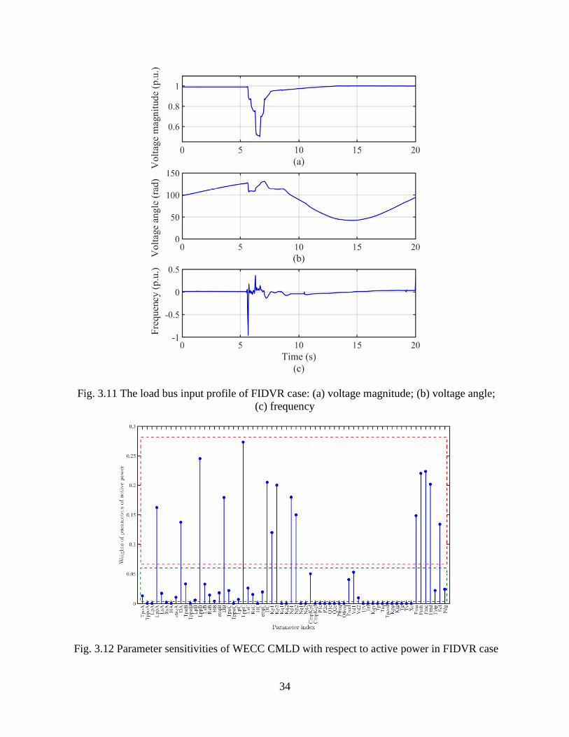
34
Fig. 3.11 The load bus input profile of FIDVR case: (a) voltage magnitude; (b) voltage angle;
(c) frequency
Fig. 3.12 Parameter sensitivities of WECC CMLD with respect to active power in FIDVR case

35
Fig. 3.13 The parameter sensitivities of WECC CMLD with respect to reactive power in FIDVR
case
Comparing the parameter sensitivity results in Fig. 3.12 and Fig. 3.13 with Case I, we can find that
the parameters of single-phase motor become sensitive. This can be attributed to that the single-
phase motor plays an important role in capturing the dynamics during the delayed-recovery stage.
Same as in Case I, 20% of perturbation is added to three parameter sets: parameters with lowest
sensitivities (outside all the rectangles in Fig. 3.12 and Fig. 3.13), parameters with lower
sensitivities (outside the red rectangles), and most sensitive parameters (inside the red rectangles).
The comparison results in Fig. 3.14 and Fig. 3.15 show that the output of interest is altered
significantly in the calculated sensitive direction but is almost not influenced when perturbing the
insensitive parameters. This verifies the effectiveness of our method on FIDVR case.

36
Fig. 3.14 Validation of PR result for real power of WECC CMLD, with different combinations
of parameters perturbed by twenty percent
Fig. 3.15 Validation of PR result for reactive power of WECC CMLD, with different
combinations of parameters perturbed by twenty percent
3.4.3 Case III: Comparison with Three Classical PR methods
In this subsection, the proposed ASM method is compared with three representative and widely-
used methods: FWKL method [101], Sobel method [97] and Morris method in [89]. The
regularization parameter λ of FWKL is chosen as 100. The sample size of Monte Carlo simulation
for Sobel method is selected as 1500SobelM = . The times of repetition for Morris method is selected
as 15MorrisM = . The other simulation setups are the same as in Case I. Since the results of active

37
and reactive power are consistent, for simplicity, only the results of active power are shown here.
Fig. 3.16 Parameter sensitivities calculated by FWKL method. 12 parameters in the red
rectangle are considered as sensitive ones
Fig. 3.17 Parameter sensitivities calculated by Sobel method. 9 parameters in the red rectangle
are considered as sensitive ones

38
Fig. 3.18 Parameter sensitivities calculated by Morris method
Fig. 3.19 Comparison of results validation of four methods by adding 20% perturbation on: (a)
sensitive parameters; (b) insensitive parameters

39
The parameter sensitivities calculated by three methods are shown in Fig. 3.16~3.18, respectively.
In Fig. 3.18, 24 parameters outside the red rectangle are considered as sensitive ones. and
are the mean and standard deviation of the elementary effects, respectively. We can observe that,
Morris method reduces least number of parameters, while Sobel method reduces the most.
Moreover, the identified sensitive parameter indices by Sobel are the most similar to those by
ASM. The result validation is conducted by adding 20% on all sensitive and insensitive parameters
sets, respectively. From Fig. 3.19, we can observe that, the blue line (ASM) deviates farthest away
from the black line (original) in the sensitive direction, and is closest to that in the insensitive one.
This indicates that ASM is the most accurate among the four methods for this case.
Table 3.2 Comparison of key features of the four PR methods
Category Accuracy Interaction Computation
ASM Gradient, Monte
Carlo Accurate Quantitative 2 ASMmM
FWKL Optimization Rough Qualitative Depends
SOBEL Variance, Monte
Carlo Accurate Quantitative ( 2)SobelM m +
Morris OAT Rough Qualitative ( 1)MorrisM m +
Fig. 3.20 Comparison of convergence rates of: (a) ASM; (b) Sobel

40
Some key features of the four methods can be concluded as Table. 3.2. Note that the computational
cost of ASM, Sobel and Morris are considered in terms of the number of experiments. FWKL is
optimization-based, thus its computational cost depends on the numbers of both iterations and
experiments, which makes it take more time than the other three methods. To further compare the
computational cost of ASM and Sobel methods, we sequentially increase the Monte Carlo sample
sizes to observe the converge rate of parameter sensitivities. Fig. 3.20 shows that the sensitivities
obtained by ASM converge after 500 samples, while Sobel needs about 1500 ones. As a
conclusion, the ASM is the most accurate with relatively lower computational cost (than Sobel and
FWKL methods).
3.5 Summary
A novel PR approach for the WECC CMLD is proposed based on ASM. With this approach, the
sensitivities of parameters are computed while the interdependency among the parameters is taken
into consideration. By applying the proposed algorithm to the WECC CMLD, the dimensions of
parameter spaces can be significantly reduced. The PR result is validated by sufficient summary
plot and perturbation tests with different voltage cases. The comparison with other classical
methods has shown the advantages of the proposed method.
Note that the ASM requires scalar function which limits its application to vector-valued
parameterized model whose output is ,T
P Q . Therefore, it cannot be directly used to analyze the
parameter sensitivity for both real and reactive power simultaneously. One may use a scalar to
combine them, however such output of interest may lack the physical meaning. We would like
trying to extend the scalar ASM to deal with vector-valued functions in the future work.

41
4. WECC Composite Load Model Parameter Identification using
Evolutionary Deep Reinforcement Learning
4.1 Introduction
Parameter identification of load models is essential to power systems studies, such as planning,
operation and control [81],[85],[103],[111]. Due to the increasing diversity of load types and the
integration of distributed energy resources (DERs) [112],[113], parameter identification still
remains a challenging problem to academic researchers and industrial practitioners. Measurement-
based approaches are widely employed to perform parameter identification, where voltage and
power measurements in fault-induced delayed-voltage-recovery (FIDVR) events are used to
determine the parameters of given dynamic load models.
Previous works have mainly focused on identifying parameters of a composite load model which
consists of a ZIP and an induction motor, where ZIP model is a combination of a constant-
impedance load, a constant-current load and a constant-power load. In [103], based on trajectory
sensitivities, the induction motor parameter number is reduced and only critical parameters are
identified. The proposed approach is validated using real field measurements, and it is
demonstrated that the approach can decrease identification time without losing the composite load
model’s dynamic characteristics. In [114], a robust time-varying parameter identification approach
is proposed for synthesis load modeling. The synthetic load model includes time-varying ZIP,
induction motor, and equivalent line impedance model. To achieve the goal of robustness
enhancement, dynamic programming is used to detect voltage disturbances, and then a time-
varying parameter identifier with a smaller iteration threshold is designed. In [115], a multi-modal
long short-term memory deep learning method is employed to identify the time-varying parameters
of the composite load model. In [116], a computationally efficient technique is utilized for
identifying the composite load model parameters, by performing a similarity analysis of parameter
sensitivity. The partial derivative of each parameter is employed to identify parameters with
similar sensitivities, and Levenberg-Marquardt algorithm is used to solve the optimization
problem. To improve computational efficiency, in [117], model parameter sensitivities are
analyzed using eigenvalues of Hessian matrix, and the linear dependence between two parameters
are then identified by examining the condition number of the Jacobian matrix. In [82], a robust
time-varying parameter identification approach is developed for the composite load model. A
batch-mode regression form is constructed to guarantee data redundancy, and the down-weighting
coefficient for each measurement is calculated to reduce the impacts of outliers. To sum up, in
previous works, both traditional optimization methods and modern learning-based approaches are
employed to perform parameter identification of the composite load model which consists of a ZIP
model and an induction motor model.
In recent years, as a large number of DERs are integrated into distribution systems, the composition
of loads has changed significantly [118]-[120]. In order to accurately capture the characteristics of
this new type of load in modern power grids, the Western Electricity Coordinating Council
(WECC) has developed a composite load model with distributed generation (CMPLDWG) [121].
Also, researchers have dedicated great efforts into studying this newly-proposed advanced load
model. In [8], an easy-to-use tool is developed to generate dynamic load data to enhance utilities’
planning studies. This tool can be adjusted to accommodate different customer types, various load

42
components and characteristics. In [85], a generic modeling and open-source implementation of
the WECC composite load model are presented, which reduces the gap between the WECC model
and its further implementation. In [81], an approach is proposed for dynamic composite load
modeling, where parameter dependency of the complex dynamic load model is analyzed and
visualized using matrix decomposition and data clustering techniques. Meanwhile, the parameter
identification performance is improved by adding a regularization term to include apriori
parameter information into the objective function. However, the apriori parameter information is
not generally available. In addition, the newly-approved aggregated distributed energy resources
(DER_A) model in CMPLDWG has not been considered in [81]. In [122], the parameter
identification process is divided into two steps: determining load composition and selecting a best-
fit parameter vector candidate from Monte-Carlo simulations. To sum up, the primary
disadvantages of previous WECC model parameter identification approaches are that they rely on
prior knowledge of parameters or a comprehensive library of parameter candidates.
The CMPLDWG model contains 183 parameters, and the order of differential equations reaches
25. Therefore, the traditional optimization methods might not be able to handle the high-
dimensional parameter vector and the severe nonconvexity of model structure. Considering this,
we seek to perform parameter identification for CMPLDWG using an advanced learning-based
approach with an embedded intelligent exploration (IE) mechanism, which is inspired by the
evolutionary deep reinforcement learning (EDRL) technique. The proposed approach can
efficiently avoid deceptive local optima and can handle the high-dimensional parameter vector
[123],[124]. Specifically, first, the parameter sensitivity analysis (PSA) is conducted to obtain
sensitivity weights reflecting contributions of parameters to dynamics, using feature-wise
kernelized Lasso (FWKL), where Lasso denotes the least absolute shrinkage and selection
operator. Then, the extracted parameter sensitivity weights are integrated into EDRL with IE to
perform intelligent CMPLDWG parameter exploration by avoiding purely randomized or
ineffective search. Parallelly, the EDRL with IE performs parameter exploitation using
evolutionary strategy. Finally, the EDRL with IE guides the identifier to balance exploitation and
exploration by designing time-varying dynamic weights assigned to the approximated
performance gradient and novelty gradient.
The main innovations and contributions of the work in this chapter are summarized as follows: (1)
To address the challenges of parameter identification caused by the nonlinearity of CMPLDWG
model, we have designed a mechanism of intelligent exploration for encouraging the parameter
identifier to escape from deceptive local optima. The exploration mechanism is achieved through
time-varying dynamic weights which intelligently balance the exploitation and exploration. Most
importantly, once the parameter identifier is stuck in a local optimum, it is stimulated to
aggressively explore undiscovered parameter space. (2) The extracted CMPLDWG parameter
sensitivity weights are innovatively integrated into the intelligent exploration to achieve directed
and efficient parameter space discovery. By doing this, the parameter identifier can avoid purely
randomized or inefficient exploration.

43
4.2 CMPLDWG Model and Overall Parameter Identification
4.2.1 CMPLDWG Model
This chapter focuses on the comprehensive WECC composite load model, which consists of three
sections: substation, feeder and load, as illustrated in Fig. 3.1. The substation section is com-posed
of a transformer model and a shunt capacitor model. The feeder section is denoted using an
equivalent feeder model. The load section includes three three-phase induction motor models with
different dynamic characteristics, one single-phase A/C performance-based motor model, an
electronic load model, a static load model and a distributed generator model. In this chapter, the
distributed generator model is specified as the newly-approved DER_A model presented in
[107][21]. Table I shows a list of WECC CMPLDWG model parameters of which detailed
definitions can be found in [121],[107]. In addition, the mathematical state-space representations
of CMPLDWG model are presented in [110].
4.2.2 Overall Framework of the Proposed Approach
The process of identifying unknown CMPLDWG parameters comes down to finding optimal
parameters by reducing the following estimation residual [81]:
( ) ( )( )2
2
1min min , .
2 , , Yl Y V f V
= − (4.1)
where, Y denotes active/reactive power measurement vector, represents the vector of
parameters to be identified, V denotes voltage measurement vector, l represents calculating the
estimation residual, 2 is the 2l -norm, and ( )f denotes the mathematical representation of
CMPLDWG model developed in [110]. More detailed variable definitions will be elaborated in
Section 4.3. To determine the optimal parameters for CMPLDWG, the EDRL approach with IE is
developed in this chapter.
Fig. 0.1 Overall structure of the proposed parameter identification approach for CMPLDWG
model

44
The components of parameter identification framework are illustrated in Fig. 4.1: Component I -
Sensitivity Analysis: Sensitivity analysis evaluates the contributions of parameters to dynamic
power measurements, and is based on the observation that the change of some parameters has an
insignificant impact on power measurements. The high-order characteristic of induction motors
and DER_A in CMPLDWG can significantly complicate PSA when using traditional methods. To
address this challenge, an alternative data-driven PSA approach, FWKL, is proposed. The FWKL
utilizes a set of randomly-generated CMPLDWG parameter vectors and corresponding calculated
residuals to extract weights indicating parameter sensitivities. The PSA is formulated as a Lasso
optimization problem given as
2
12min .
1
2d
T
We W W
− +
¡ (4.2)
where, e is the estimation residual vector, denotes the randomly-generated parameter vectors
in a matrix form, 1, ,T
dW W W= K represents the parameter sensitivity weight vector, 1 is the
1l -norm and is the regularization parameter which is determined using grid search with cross-
validation. Note that sensitivity analysis is a one-off work for each fault event. The extracted
parameter sensitivity weight vector, W, is passed to the novelty gradient estimator in each iteration
whose number is denoted by t. Component II - Parameter Vector Perturbator: In each iteration, to
per-form evolution, a perturbator is designed to generate multiple mutated parameter vectors, '
t
’s, using the identified parameter vector in the last iteration, t , and random variance vector, t . '
t ’s and t ’s are then sent to a performance gradient estimator and a novelty gradient estimator to
approximate performance and novelty gradients, respectively. Component III - Performance
Gradient Estimator: This estimator achieves the function of exploitation of EDRL. Specifically,
using '
t ’s and t ’s generated by the parameter vector perturbator, the performance gradient
estimator determines the direction in which t should move to improve expected reward. The
performance gradient, et
t , is then passed to a parameter updater. Component IV - Novelty
Gradient Estimator: This component performs exploration by estimating the novelty gradient, er
t , using the generated '
t ’s and t ’s, and it also intelligently encourages the parameter
identifier to explore unvisited parameter space. er
t is then sent to the parameter updater.
Component V - Parameter Updater: To balance exploitation and exploration, the parameter updater
assigns time-varying dynamic weights to the approximated performance and novelty gradients:
( )1 ,et er
t t t t t = + − (4.3)
where, t denotes a dynamic weight. Then, 1t + is calculated and added into the parameter vector
archive to update the explored parameter space. Component VI - Archive: The archive collects the
previously generated parameter vectors which are passed to the novelty gradient estimator for
novelty evaluation. Component II to V compose the EDRL algorithm with IE. Since the
construction of the parameter vector archive is straightforward, we will focus on elaborating the
modules of sensitivity analysis and EDRL with IE in the next two sections.

45
4.3 Parameter Sensitivity Analysis
PSA examines the sensitivity of dynamic power measurements with respect to load model
parameters. In previous works, partial derivative of dynamic power to each parameter is calculated
to conduct sensitivity analysis of induction motor parameters [116]. However, it becomes
challenging to directly apply analytical approaches to calculate partial derivatives because of the
high order and the complicated structure of mathematical differential equations of the WECC
composite load model. For example, the three-phase induction motor model in CMPLDWG is of
5th order and the DER_A model has ten state variables. Such a complex high-order nonlinear
system can significantly complicate the calculation of partial derivatives. To address this
challenge, we seek to employ a high-dimensional feature selection technique to evaluate the
dependence of dynamic power on the CMPLDWG parameters [125]. Specifically, we use a data-
driven FWKL instead of employing analytical derivatives [116].
Let d
i ¡ be a randomly-generated parameter vector and d be the number of parameters,
therefore, the power residual corresponding to i can be calculated as
( )2
, ,i ie f V Y= − (4.4)
where, KV ¡ is a vector of voltage measurements, K denotes the total number of measurement
points, ,T
T TY P Q = , KP ¡ and KQ ¡ represent the vector of recorded active power and
reactive measurements, respectively. Also, T denotes the transpose. With a large number of
generated i ’s, we can obtain n independent and identically distributed (i.i.d.) sample and residual
pairs:
( ) , , 1, , .i ie i n = K (4.5)
To perform supervised feature selection, first, we represent the original parameter vectors and
corresponding residuals in a matrix format as
1, , ,d n
n = K ¡ (4.6a)
1, , .T n
ne e e= K ¡ (4.6b)
Then, PSA is formulated as a Lasso optimization problem formulated in (4.2) which works well
for linear regression. However, the nonlinear dependency in our specific problem hinders its
application. Therefore, we employ the feature-wise nonlinear Lasso to solve our problem and the
key idea is to apply a nonlinear transformation in a feature-wise manner. Specifically, the generated
parameter matrix, , is represented in a feature-wise manner:
1, , ,T d n
d = K ¡ (4.7)
where, ,1 ,, ,T n
k k k n = K ¡ is a vector denoting the k-th feature for all samples. To capture

46
the nonlinear dependency of e on , dynamic power residual and parameter vector are
transformed by a nonlinear function ( ) : n p →¡ ¡ . Then, the Lasso optimization problem given
in the objective function (4.2) in the transformed space is reformulated as
( ) ( )2
11 2
1min .
2d
d
k kW
k
e W W
=
− +¡
(4.8)
Although the objective function (4.8) can capture nonlinear dependency, there is no constraint for
, 1, ,kW k d= K , and the same transformation function ( ) for e and k limits the flexibility of
capturing nonlinearity. To solve this, we seek to employ a revised FWKL to perform feature
selection [125], and the revised objective function is formulated as
( )2
11
1min ,
2d
dk
kW
k Frob
U W V W
=
− +¡
(4.9a)
1. . , , 0.ds t W W K (4.9b)
where, Frob denotes the Frobenious norm, U U= and
( ) ( )k kV V= are centered Gram
matrices, ( ), ,i j i jU U e e= and ( ) ( ), , ,,k
i j k i k jV V = are Gram matrices, ( ), 'U e e and ( ), 'V e e are
kernel functions, 1
1 1T
n n nIn
= − denotes the centering matrix, nI represents the n-dimensional
identity matrix, and 1n denotes the n-dimensional vector with all ones. For the two kernel functions
( )U and ( )V , we employ the Gaussian kernel which is formulated as
( )( )
2
2
', ' exp ,
2 x
x xK x x
−= −
(4.10)
where, x is the Gaussian kernel width.
In the objective function (4.9a), the decoupling between ( )U and ( )V provides more flexibility
compared with the objective function (4.8). In addition, the non-negativity constraint in (4.9b) fits
the specific application in our problem, since negative sensitivity parameter weights do not have
practical interpretability. Intuitively, problem (4.9) tends to find non-redundant parameters with
significant contributions to power residual, and equivalently, to dynamic power. Also, for two
strongly dependent features, either of their sensitivity weights tends to be eliminated. The
parameter sensitivity weight vector, W, is then integrated into the parameter identification
algorithm to accelerates the learning process, which will be presented in Section 4.4.

47
4.4 Parameter Identification using the EDRL with IE
As stated in previous sections, the severe nonlinearity, high nonconvexity and the large number of
parameters bring significant challenges to perform parameter identification for the CMPLDWG
model when using existing approaches. This motivates us to tackle this challenge utilizing the
EDRL with IE, which is recently demonstrated to be able to perform well on high-dimensional
optimization tasks [123],[126]. The basic idea of performing optimization tasks using evolution
strategy is: During each iteration, a population of parameter vectors is perturbed based on one
selected parameter vector among a meta-population, and then, these mutated vectors are
recombined to update the selected ancestor vector. In this chapter, the EDRL is also hybridized
with IE to improve exploration. Compared with traditional random and blind search strategy, the
IE module achieves efficient and directed exploration, which can efficiently assist EDRL to escape
from local optima. The detailed steps are described as follows:
Fig. 0.2 Detailed structure of the EDRL with an intelligent exploration mechanism

48
Step I - Initialization: The first step is to initialize M random parameter vectors which will be
updated in each iteration. Note that only one vector is probabilistically selected to update in each
iteration. The initialized M vectors are denoted as 1
1 1, , MS = K , where t denotes the number of
iteration. The objective of constructing a meta-population is to enhance additional diversity. M and
the tuning parameters in the remaining sections are determined using grid search with cross-
validation which is a general hyperparameter optimization technique.
Step II - Sampling: In each iteration t, we probabilistically determine which parameter vector
among the M meta-population to be updated based on parameter vectors’ novelties. The novelty is
evaluated in terms of Euclidean distances from a vector to the vectors in the newest archive.
Specifically, first, the originality of each parameter vector in S, k
t , conditioned on current
parameter vector archive, A, is evaluated as
( ) ( )2
1, , . ,k k k
t t t j
j C
O o W A WC
= = − (4.11)
where, 1 ≤ k ≤ M, ( ) 1 ', , ,k
t NC kNN A = = K , kNN denotes k-nearest neighbors algorithm,
and .* denotes the element-wise multiplication operation. The purpose of kNN is to select
representative parameter vectors in A for evaluating the novelty of k
t . Intuitively, a small k can
introduce higher distance variance, while a large k means higher computational cost. We have
conducted numerical experiments to determine the optimal k value which is sufficient for
evaluating the novelty of a newly explored parameter vector while avoiding high computational
time. The intro-duction of W, which is obtained from PSA, aims to revise Euclidean distances
between vectors. This revision is based on the consideration that parameters with different
sensitivity weights have different contributions to vector novelty. Then, for each parameter vector
in S, the novelty score which determines the probability of being selected to be updated is
calculated as
1
.k
k tt M j
tj
OP
O=
=
(4.12)
k
tP tells us that selecting the parameter vectors with high novelty scores can achieve directed or
guided exploration.
Step III - Variation: In this step, variation is performed on the selected parameter vector in Step II, k
t , to generate multiple workers. The function of these workers is explained as follows: First,
EDRL produces parameter vectors in the neighborhood of k
t , and then k
t is updated by
following the direction determined by the population of the produced parameter vector workers.
To obtain N workers, Gaussian noise is applied to k
t as follows
, 1, , ,i k k i
t t t i N = + = K (4.13)

49
where, is a fixed noise standard deviation, ( )0,i
t I : and I is an N-dimensional identity
matrix.
Step IV - Gradient Estimation: In this step, the performance and novelty gradients determined by
the meta-population of generated vectors in Step III are approximated. For each mutated parameter
vector, ,i k
t , its fitness can be evaluated via calculating the difference between the estimated
dynamic power and the real dynamic power. First, the power residual caused by the mismatch
between estimated parameters and real parameters, ,i k
te , is calculated by substituting ,i k
t into
(4.4). Then, the reward is obtained by inversing ,i k
te :
( ), ,
,
1, , 1, , ,i k i k
t t i k
t
R r V Y i Ne
= = = K (4.14)
Equation (4.14) indicates that as the residual decreases the reward increases. Thus, the
performance gradient of k
te is approximated via taking a sum of the sampled parameter vector
perturbations weighted by the reward:
, ,
1
1,
Net k i k i
t t t
i
RN
=
(4.15)
where, is a learning rate. In (4.15), ,et k
t indicates a stochastic reward experienced over a full
iteration of multiple worker interactions, which means the performance gradient relies on multiple
workers and this can effectively avoid the high variance brought by a certain single mutated vector.
Note that the calculated reward, ,i k
tR , is normalized through 1 to N before performing the gradient
approximation in (4.15).
For the novelty gradient, first, the novelty with respect to each perturbed vector, ,i k
tO , is calculated
using (4.11). Then, the novelty gradient of k
t is approximated as
, ,
1
1,
Ner k i k i
t t t
i
ON
=
(4.16)
Similar with ,i k
tR , ,i k
tO , is normalized before computing the novelty gradient. Intuitively, ,er k
t
indicates the direction which the parameter identifier should follow to increase the average
originality of parameter vector distribution.
Step V - Gradient Combination: Using the computed performance and novelty gradients with
respect to k
t , we can balance exploitation and exploration by introducing a time-varying dynamic
weight, t . Thus, the overall gradient based on which k
t should be updated is computed as
follows:
( ), ,1 ,k et k er k
t t t t t = + − (4.17)

50
Intuitively, the algorithm follows the approximated gradient in parameter-space towards directions
that both exhibit novel behaviors and achieve high rewards. A large t tends to encourage k
t to
follow the performance gradient and restrain it to follow the novelty gradient. In comparison, a
small t tends to aggressively guide k
t to mutate to unseen parameter space and hold back
exploitation.
Step VI - Updating: After obtaining k
t , the updating of k
t is expressed as follows:
1 ,k k k
t t t + = + (4.18)
1
k
t + is then added into the archive A for updating the pre-existing vector landscape. As more
learned parameter vectors are saved into A, the base for evaluating future parameter vectors’
novelty changes and stimulates the algorithm to discover unexplored parameter space.
In addition to updating k
t and A in each iteration, the dynamic weight, t , should also be updated
for avoiding local optima. To do this, first, the latest reward, 1
k
tR + , which is brought by 1
k
t + , is
calculated. We also define a “drag hand”, t
bR , to record the best reward among historical rewards.
Then, the dynamic weight in (4.17), t , is updated using Algorithm 1, where, denotes the
weight updating rate, and t
bC counts the number of rewards that are less than t
bR in succession.
setC is a threshold which determines the frequency of updating t when the parameter vector is
stuck in a local optimum. Also, t
bC and t
bR are updated in each iteration, as presented in Algorithm
1. Note that Step II to VI constitute the entire operation in each iteration t.
4.5 Case study
In this section, the proposed parameter sensitivity analysis and parameter identification algorithms
are validated using numerical experiments. Before performing verification, we firstly screen out
the CMPLDWG parameters that are necessary to be identified. This screening is based on the
consideration that CMPLDWG contains multiple types of parameters, of which some parameters
can be determined by field measurements and engineering judgement. Specifically, the transformer
impedance, substation shunt capacitive susceptance, feeder impedance and capacitive susceptance
can be accurately calculated using transformer, capacitor and feeder parameters [127],[128]. For
the stalling and restarting of induction motors, engineering judgement can be lever-aged to
estimate the settings [121],[129]. This is based on the observation that the stalling or restarting of
a large number of induction motors can cause abrupt current, voltage and power changes
[130],[131], which can be further corroborated in [81]. Also, the tripping of a large number of
induction motors can cause sudden current decrease, power decrease and voltage increase.
Excluding the parameters which can be accurately calculated using the electric power grid
modeling technique can significantly reduce the complexity of parameter identification process.
On the other hand, indistinguishably identifying all CMPLDWG parameters can pose an
unnecessary computational burden on the proposed parameter identification algorithm. In our
problem, 61 CMPLDWG parameters are screened out for parameter identification, as shown in
Table III, and the remaining parameters are set with default values.

51
In this case study, the Power System Simulator for Engineering (PSS/E) and the ACTIVSg500 test
case are employed to generate voltage and power measurements for parameter identification [132].
The fault-induced voltage-recovery curves are shown in Fig. 4.3. MATLAB is used to execute the
processes of parameter sensitivity analysis and parameter identification. The case study is
conducted on a standard PC with an Intel Xeon CPU running at 3.70 GHz and with 32.0 GB of
RAM.
Fig. 0.3 Fault-induced voltage-recovery curves at the load bus
4.5.1 Parameter Sensitivity Identification
To fully extract the sensitivity weights hidden in the randomly-generated parameter samples and
corresponding power residuals, first, we have created a comprehensive library containing 40,000
parameter vector and residual pairs which are divided into two sections, training dataset and test
dataset, for cross-validation. Note that the dataset size is determined based on our numerical
experiment result that once the dataset size exceeds 16,000, the FWKL gives us stable extracted
parameter weights for different sets of the randomly selected parameter vector and residual pairs.
Generating each pair of the parameter vector and the corresponding residual takes about 0.3

52
seconds. Then, the tuning parameters of FWKL are determined using grid search with cross-
validation based on the training and test datasets [133]. Finally, the FWKL algorithm is applied to
the entire dataset to conduct parameter sensitivity analysis. Based on our sensitivity analysis result,
the load fraction parameters, the synchronous and sub-transient reactances of three-phase
induction motors, and the exponential load torque coefficients of three-phase induction motors
have a significant effect on the load dynamics in the fault event specified in Fig. 4.3, as shown in
Fig. 4.4. The remaining parameters have small or no effect on the dynamic procedure. It should be
noted that the values of parameter sensitivity weights change according to specific dynamic events
since the weight vector in (4.9) partially depends on the voltage and power measurements, which
are determined by specific fault cases. Therefore, PSA should be conducted on a case-by-case basis
to obtain more accurate parameter sensitivity weights for specific fault events.
Fig. 0.4 Sensitivity weights of WECC composite load model parameters
4.5.2 Parameter Identification
The extracted parameter sensitivity weights are integrated into EDRL algorithm with IE to perform
parameter identification using given voltage and power measurements. There are only a couple of
published technical reports involved with WECC model parameter settings. In this case, the
numerical intervals of parameters for randomly selecting initial values are determined based on
[134],[135], along with our experience on deriving detailed mathematical representation of WECC
composite load model [110]. The numerical intervals are presented in Table 4.1, where, LB
denotes lower bound and UB denotes upper bound. Table 4.2 shows the real and corresponding
identified parameter values of CMPLDWG. As can be observed, the EDRL with IE can give us
satisfying identified parameters. The identification accuracy is further corroborated by Fig. 4.5, in
which, the estimated active and reactive power curves can closely fit the actual curves. While our
approach is not designed for online parameter identification, it is of importance to examine the
computational time. In our case studies, each iteration takes about 2 seconds.

53
Table 0.1 Numerical interval of load parameters
Parameter LB UB Parameter LB UB Parameter LB UB
Motor A LppC 0.06 0.24 Electronic Load
TpoA 0.046 0.184 LsC 0.9 3.6 Frcel 0 0.38
TppoA 0.001 0.004 RsC 0.015 0.06 DER_A
LpA 0.05 0.20 HC 0.1 0.4 Trv 0.01 0.04
LppA 0.042 0.168 EtrqC 1.8 2.2 Trf 0.02 0.06
LsA 0.9 3.6 DC 0.5 2.0 Kqv 0.5 2
RsA 0.02 0.08 Motor D Tp 0.01 0.04
HA 0.05 0.20 Kp1 0 1 Tiq 0.01 0.04
EtrqA 0.5 2.0 Kp2 6 24 Tpord 2.5 10
DA 0.5 2.0 Kq1 3 12 Kpg 50 200
Motor B Kq2 5.5 22 Kig 5 20
TpoB 0.05 0.20 Np1 0.5 2 Tg 0.01 0.04
TppoB 0.001 0.005 Np2 1.6 4.8 Tv 0.01 0.04
LpB 0.08 0.32 Nq1 1 4 Xe 0.13 0.5
LppB 0.06 0.24 Nq2 1.25 5 Load Fraction
LsB 0.9 3.6 CmpKpf 0 2 Fma 0 0.5
RsB 0.015 0.06 CmpKqf -6.6 -1.6 Fmb 0 0.5
HB 0.5 2.0 Static Load Fmc 0 0.5
EtrqB 1 3 P1c 0 0.4 Fmd 0 0.5
DB 0.5 2.0 P2c 0 0.6 Fel 0 0.5
Motor C Q1c 0 0.4 Fdg -0.5 0
TpoC 0.05 0.20 Q2c 0 0.6 Fzip 0 0.5
TppoC 0.001 0.005 Pfreq -0.2 0.2
LpC 0.08 0.32 Qfreq -2 -0.5

54
Table 0.2 Real and identified CMPLDWG parameters
Parameter Real Identified Parameter Real Identified Parameter Real Identified
Motor A LppC 0.12 0.1064 Electronic Load
TpoA 0.092 0.0906 LsC 1.8 1.7535 Frcel 0.25 0.1551
TppoA 0.002 0.0024 RsC 0.03 0.0286 DER_A
LpA 0.1 0.1037 HC 0.2 0.2839 Trv 0.02 0.0262
LppA 0.083 0.0495 EtrqC 2 2.3741 Trf 0.03 0.0221
LsA 1.8 1.8637 DC 1 1.0687 Kqv 1 1.4408
RsA 0.04 0.0275 Motor D Tp 0.02 0.0207
HA 0.1 0.1188 Kp1 0 0.8636 Tiq 0.02 0.0153
EtrqA 1 0.8368 Kp2 12 11.675 Tpord 5 4.0030
DA 1 0.9661 Kq1 6 8.0773 Kpg 100 68.3279
Motor B Kq2 11 10.950 Kig 10 9.9675
TpoB 0.1 0.0883 Np1 1 1.3602 Tg 0.02 0.0156
TppoB 0.0026 0.0034 Np2 3.2 4.4470 Tv 0.02 0.0163
LpB 0.16 0.1094 Nq1 2 1.6632 Xe 0.25 0.2239
LppB 0.12 0.1797 Nq2 2.5 2.5239 Load Fraction
LsB 1.8 2.0663 CmpKpf 1 0.5 Fma 0.2 0.1969
RsB 0.03 0.0302 CmpKqf -3.3 -4.2400 Fmb 0.3 0.4393
HB 1 1.4290 Static Load Fmc 0.3 0.3113
EtrqB 2 2.4816 P1c 0.2 0.1953 Fmd 0.1 0.1300
DB 1 1.2146 P2c 0.3 0.2094 Fel 0.2 0.1804
Motor C Q1c 0.2 0.1588 Fzip 0.1 0.1774
TpoC 0.1 0.0941 Q2c 0.3 0.1727 Fdg -0.2 -0.2053
TppoC 0.0026 0.0034 Pfreq 0 -0.0942
LpC 0.16 0.1268 Qfreq -1 -0.8593
It is also of significance to examine the collected best reward t
bR and dynamic weight t in each
iteration, which are shown in Fig. 4.6 and 4.7, respectively. In Fig. 4.6, the loss corresponding to
the collected best reward, t
be , is also shown for examining parameter identification performance.
It can be seen that during Iteration 1 to 1226, the proposed parameter identification approach
simultaneously performs exploitation and exploration, and the best reward increases continuously,
as shown in Fig. 4.6.

55
Fig. 0.5 The real power curves and the estimated power curves using the identified parameters
Fig. 0.6 The best reward and corresponding loss
The corresponding learning process in this iteration range can be confirmed in Fig. 4.7, in which
t is firstly initialized as 0, once it stays invariant for 10 continuous iterations ( setC ), it is decreased
in a step size of 0.05 ( ) to force the parameter identifier to follow more closely with novelty
gradient. Once an unseen better reward occurs, t gradually increases to 1 to encourage the
identifier to act following the approximated performance gradient. During Iteration 1 to 1226,
although t alternatively decreases and increases, it does not reach 0. From Iteration 1227 to

56
1717, the parameter identifier is stuck in a local optimum and the best reward stays invariant, as
shown in Fig. 4.6. During this iteration range, first, t is designed to gradually decrease to 0,
which means the identifier is stimulated to explore more aggressively in the unseen parameter
space, as presented in Section IV. This is verified by the variation of dynamic weight t , as shown
in Fig. 4.7, where, from Iteration 1227 to 1717, t decreases to 0 and keep unchanged, which
means the identifier completely inhibits the performance gradient. At Iteration 1718, the identifier
discovers a parameter vector which can give higher reward than any of the previous best rewards.
As expected, t immediately jumps to 1 to avoid possible sliding out from the newly explored
optimum with higher reward, due to novelty exploration inertia. From Iteration 1718 to 2342, the
identifier simultaneously performs exploitation and exploration as shown in Fig. 4.6, accordingly,
t varies in the range of a non-zero value to 1, as shown in Fig. 4.7. This is simi-lar to the process
which occurs in the range of Iteration 1 to 1226. Similar with the range of Iteration 1227 to 1717,
in the range of Iteration 2343 to 3324, t decreases to 0 and t
bR stays invariant, as shown in Fig.
4.7 and 4.6, respectively. At Iteration 3325, t jumps to 1 to force the identifier immediately per-
form exploitation, which is similar at Iteration 1718, as shown in Fig. 4.7. Also, the best reward
starts to increase at Iteration 3325, as shown in Fig. 4.6. The aforementioned cyclic process
continues to pursue better rewards as the number of iterations increases, as shown in Fig. 4.6 and
4.7.
Fig. 0.7 Variation of the time-varying dynamic weight
It is interesting to examine the efficaciousness of integrating sensitivity weights into the IE module.
To do this, we perform additional CMPLDWG parameter identification using EDRL with IE
without revising parameter vector novelty scores. Fig. 4.8 shows two best reward collection curves
corresponding to EDRL with IE by integrating W and without integrating W, respectively. As can
be seen, the introduction of W accelerates the exploitation and exploration in reaching the same
best reward.

57
Fig. 0.8 The introduction of parameter sensitivity weights into EDRL with IE improves learning
performance
Fig. 0.9 Performance comparison of EDRL, SSA and DQN
It is also significant to compare the proposed parameter identification approach with the presented
algorithms in previous works. First, we focus on comparing our algorithm with the proposed
parameter identification approach in [81], which also aims to identify a large number of
parameters. The comparison shows that our approach can achieve better parameter identification
accuracy and does not rely on apriori knowledge. And also, our method is easier to implement due
to the utilization of mathematical representation of CMPLDWG model. In addition, the parameter
identification accuracy using the proposed approach in [81] significantly relies on apriori
knowledge about parameter setting. We have also compared the performance of our proposed
approach with that of two other state-of-the-art optimization algorithms, Salp Swarm algorithm
(SSA) and deep Q-networks (DQN). SSA is a newly proposed metaheuristic optimizer inspired by
the process of looking for a food source by salps. SSA has demonstrated satisfying performance
compared with other metaheuristic algorithms [136]. DQN is a cutting-edge reinforcement
learning technique designed for sequential decision-making tasks [137]. The performance of the
three algorithms (EDRL, SSA and DQN) is shown in Fig. 4.9. It can be seen that our proposed

58
approach outperforms the other two methods in terms of the average fitness error, t
be . In
comparison, SSA shows the fastest convergence rate. DQN takes the longest time to converge and
shows the largest average fitness error. It is also important to point out that DQN needs a
significantly longer time to train a stable actor with satisfying identification performance.
4.6 Summary
This chapter presents a parameter identification approach for WECC composite load model. The
proposed method employs a data-driven nonlinear feature selection technique to perform
parameter sensitivity analysis, which avoids solving highly complex analytical derivatives caused
by the high order and nonlinearity of differential equations of WECC composite load model. After
that, the proposed method utilizes a cutting-edge approach inspired by evolutionary reinforcement
learning technique, which is hybridized with an intelligent exploration mechanism to perform
parameter identification. The parameter sensitivity weights are innovatively embedded in the
reinforcement learning process to achieve efficient exploration. The numerical experiments
demonstrate that the proposed approach can achieve promising accuracy. It is also shown that the
proposed identifier can escape from local optima through the assistance of the intelligent
exploration mechanism when stuck in local optima. Finally, it is verified that the integration of
sensitivity weights into the reinforcement learning process accelerates the learning rate.
While our proposed approach can perform parameter identification of WECC composite load
model with satisfying accuracy, the computational cost hinders its online application. Also, the
model complexity stands in the way of widely applying WECC composite load model in the
electric power industry. Considering this, one prospect for research on CMPLDWG is to simplify
the model or develop a surrogate model to significantly reduce the computation cost and/or model
complexity, while keeping the primary characteristics of WECC model.

59
5. Python-PSSE-Combined Autonomous Parameter Identification Program
5.1 Introduction
The WECC composite load model is widely used in power system stability analysis, energy
conservation, and power system operation optimization, etc. A brief description of the WECC
composite load model (CMPLDW) is shown in Fig. 5.1. The CMPLDW consists of a bus, a feeder,
three three-phase motors, a single-phase motor, an electronic load, a static load. The transformer
and feeder contain 18 parameters, the three-phase motors contain 65 parameters, the single-phase
motor contains 34 parameters, the electronic load contains 5 parameters, and the static load
contains 11 parameters. In total, the CMPLDW has 133 parameters.
In some more advanced versions of the WECC model, a distributed generator (DG) is also
included, which forms a WECC composite load model with DG (CMPLDWG). The DG contains
46 parameters, so the CMPLDWG has 179 parameters in total.
A purpose of this project is to identify the parameters of the WECC composite load model to fit
the active and reactive power measurements using event data, and it is a pretty challenging task
considering that the WECC model is a highly nonlinear and complex load model with a huge
number of parameters. In order to identify the parameters, it is essential to have a convincing
representation of the WECC model. It is possible for the researchers/scholars to code the WECC
model in Matlab or other programming languages (e.g., python), but considering the great
complexity of the WECC model, especially those nonlinear equations and the protection actions,
it is very difficult that the WECC model coded in Matlab/python can 100% accurately represent
the characteristics of the WECC model. In such cases, some errors may in incurred by the imperfect
representation of the WECC load model. An alternative is to use the WECC load module in the
PSSE commercial software, which is believed to be the available most accurate representation of
the WECC load model. But it is worth noting that the DG is currently unmodeled in the PSSE
software.
Fig. 0.1 Brief introduction of WECC load model

60
5.2 Python-PSSE Autonomous Parameter Identification Approach
There are various kinds of optimization methods available, such as conventional methods and
heuristic methods. The conventional methods include Lagrangian relaxation, benders
decomposition, branch and bound algorithm, linear programing, and mixed-integer programming.
The heuristic methods include artificial intelligence methods and bio-inspired methods. The deep
Q-learning, asynchronous advantage actor (A3C) algorithm in the category of reinforcement
learning are good examples of artificial intelligence methods. And the particle swarm optimization
(PSO), genetic algorithm (GA), and salp swarm algorithm (SSA) are good examples of bio-
inspired optimization methods.
While the conventional optimization methods are powerful and widely applied, but they could not
be applied to solve the parameter identification problem of the WECC load model. This is because
the WECC load model is highly nonlinear and could not perform the transformation required
during the solution process of the conventional optimization methods. Rather, the heuristic
methods have a much less requirement, and they are good candidates for solving the WECC load
model parameter identification problem.
Fig. 0.2 Problem description of Python-PSSE autonomous parameter identification approach
A lot of the heuristic methods can be coded conveniently in the python environment. And the
CMPLDW model is sited in the PSSE environment. Thus, a practical problem is that how can we
establish a stable connection between the optimization methods sited in the python environment
and the CMPLDW model sited in PSSE, and how can we enable them to exchange information
efficiently for solving the WECC load model validation problem.
G L
PMU Voltage
measurements
PMU frequency
measurements
Playback
generator model
WECC
load model
Line
Salp swarm algorithmP, Q curves
PSSE environment
WECC parameters
Python environment
Fig. 0.3 Overview of Python-PSSE autonomous parameter identification approach

61
An overview of our proposed Python-PSSE autonomous parameter identification approach is
shown in Fig. 5.3. We can flexibly select various optimization methods to efficiently optimize the
CMPLDW parameters. The salp swarm algorithm [136] is used here as an example due to its high
efficiency of searching, and it is coded in python. The salp swarm algorithm mimics the behaviors
of a group of salps searching for food. Based on the current best food positions, the leader salp and
the following salps update their positions. More details about this algorithm can be found at [136].
In the PSSE environment, a dynamic power system simulation model is built, and it consists of a
generator connected to a load via a transmission line. For the generator, the playback generator
model is adopted as it allows us to inject disturbance recorded by real PMU data. For the load, the
WECC load model is adopted. For the line, the typical parameters of a short transmission line are
adopted. The SSA sends the WECC parameters to the PSSE as its inputs. Based on these WECC
parameters provided by SSA, a dynamic simulation is conducted in the PSSE using the PMU
frequency measurements and voltage measurements. After the simulation is conducted, an active
power (P) curve and a reactive power (Q) curve are obtained, and they are provided to the SSA.
The SSA then compares the simulated P, Q curves with the real P, Q measurement curves to update
the WECC parameters. When the convergence of the SSA is reached, the optimal WECC
parameters can be obtained.
Fig. 0.4 Program flowchart of Python-PSSE autonomous parameter identification approach
The program flowchart of the Python-PSSE autonomous parameter identification approach is
depicted in Fig. 5.4 and explained in detail as follows.
Start
Initialize the positions of the salp swarm
Update the WECC parameters based on the
positions of the salp swarm
Call PSSE to perform dynamic simulation
Get the errors between the simulated
curves and PMU measurements
Update food position based on the errors
Update the positions of the salp swarm
Satisfy termination?
End
Yes
No

62
• Step 1: Initialize the positions of the salp swarm. Each salp is a candidate solution of the
WECC parameter identification problem, and the dimension of a salp equals to the number
of WECC parameters to be identified. In order to better explore the searching space, it is
better that the values of the salps are randomly distributed within the allowed range.
• Step 2: As each salp is a candidate solution of the WECC parameter identification problem,
the WECC parameters are updated based on the positions of the salps.
• Step 3: Call PSSE to perform the dynamic simulation. As mentioned before, the dynamic
simulation model has a playback model generator connected to a load modeled by WECC
with a short transmission line.
• Step 4: After obtained by simulated P, Q curves, the error between the simulated curves
and real PMU measurements can be obtained. It should be noted that the objective function
of the SSA is to minimize the root mean square error shown as follows:
mi n√1
2𝑁∑ [(𝑃𝑖
𝑠𝑖𝑚 − 𝑃𝑖𝑃𝑀𝑈)
2+ (𝑄𝑖
𝑠𝑖𝑚 − 𝑄𝑖𝑃𝑀𝑈)
2]𝑁
𝑖=1 (5.1)
where 𝑃𝑖𝑠𝑖𝑚 is the simulated active power curve; 𝑃𝑖
𝑃𝑀𝑈is the active power curve by PMU;
𝑄𝑖𝑠𝑖𝑚 is the simulated reactive power curve; 𝑄𝑖
𝑃𝑀𝑈 is the reactive power curve by PMU; 𝑁
is the number of measurements. As can be seen in (5.1), the reactive power and active
power are treated equally.
• Step 5: Update food position based on the error, i.e., the position of the salp with the
minimal error is the updated food position.
• Step 6: Update the positions of the salp swarm. This step can be conducted based on the
principles of the SSA algorithm.
• Step 7: Check if the termination condition is satisfied or not. In this program, the maximum
number of iterations is used as the termination criterion. If the termination criterion is not
satisfied, the program will go to step 2 and repeat.
5.3 WECC Parameter Identification using AEP Data
Our industrial partner has provided us some real event PMU data. It is about a fault that happened
on a 138 kV line. And the fault event was recorded by PMU at a nearby 12.47 kV substation. The
recorded voltage curve and frequency deviation curves are shown in Figs. 5-5 and 5-6,
respectively. As can be seen in Fig. 5-5, there is a severe frequency drop after the fault, and the
voltage quickly recovered to normal after the fault was cleared. The fault has also resulted in some
frequency deviations concurrent with the voltage fluctuation, and it is observed in Fig. 5-6 that the
frequency deviation is not too severe, but its impact on the load modeling could not be ignored.

63
Fig. 0.5 Recorded voltage curve
Fig. 0.6 Recorded frequency deviation curve
Each of the 133 CMPLDW parameters has a specific physical meaning; thus, their initial values
should be carefully chosen. To the best of our knowledge, there are no well-established
upper/lower bounds and typical values of the 133 CMPLDW parameters in the literature. So, we
carefully check the industrial report and academic paper, including those reports written by NREL
and NERC, and obtain the initial values of the CMPLDW parameters as listed in Table 5-1. All
the parameters are within their ranges of physical meanings. These parameters provide a good
initial estimation and serve as the basis for further optimization.

64
Table 0.1 Initial CMPLDW parameters
J+
index Name Value J+
index Name Value J+
index Name Value J+
index Name Value J+
index Name Value
0 MVA -1 27 P1e 2 54 Ftr2A 0.3 81 LpC 0.19 108 Np1 1
1 SubstB 0 28 P1c 0.3 55 Vrc2A 0.1 82 LppC 0.14 109 Kq1 6
2 Rfdr 0.04 29 P2e 1 56 Trc2A 999 83 TpoC 0.2 110 Nq1 2
3 Xfdr 0.04 30 P2c 0.7 57 MtypB 3 84 TppoC 0.0026 111 Kp2 12
4 Fb 0.75 31 Pfrq 0 58 LFmB 0.75 85 HC 0.1 112 Np2 3.2
5 XXf 0.08 32 Q1e 2 59 RaB 0.03 86 EtrqC 2 113 Kq2 11
6 Tfixhs 1 33 Q1c -0.5 60 LsB 1.8 87 Vtr1C 0 114 Nq2 2.5
7 Tfixls 1 34 Q2e 1 61 LpB 0.19 88 Ttr1C 999 115 Vbrk 0.86
8 LTC 0 35 Q2c 1.5 62 LppB 0.14 89 Ftr1C 0 116 Frst 0.3
9 Tmin 0.9 36 Qfrq -1 63 TpoB 0.2 90 Vrc1C 999 117 Vrst 0.95
10 Tmax 1.1 37 MtypA 3 64 TppoB 0.0026 91 Trc1C 999 118 CmpKpf 1
11 Step 0.00625 38 LFmA 0.75 65 HB 0.5 92 Vtr2C 0 119 CmpKpf -3.3
12 Vmin 1.025 39 RsA 0.04 66 EtrqB 2 93 Ttr2C 999 120 Vc1off 0.5
13 Vmax 1.04 40 LsA 1.8 67 Vtr1B 0 94 Ftr2C 0 121 Vc2off 0.4
14 Tdelay 30 41 LpA 0.12 68 Ttr1B 999 95 Vrc2C 999 122 Vc1on 0.65
15 Tstep 5 42 LppA 0.104 69 Ftr1A 0 96 Trc2C 999 123 Vc2on 0.55
16 Rcmp 0 43 TpoA 0.095 70 Vrc1B 999 97 Tstall 0.0333 124 Tth 7
17 Xcmp 0 44 TppoA 0.0021 71 Trc1B 999 98 Trestart 0.3 125 Th1t 0.4
18 FmA 0.237 45 HA 0.1 72 Vtr2B 0 99 Tv 0.025 126 Th2t 3
19 FmB 0.119 46 EtrqA 0 73 Ttr2B 999 100 Tf 0.1 127 Fuvr 0
20 FmC 0.1 47 Vtr1A 0.65 74 Ftr2B 0 101 CompLF 1 128 UVtr1 0
21 FmD 0.24 48 Ttr1A 0.2 75 Vrc2B 999 102 CompPF 0.98 129 Ttr1 999
22 Fel 0.162 49 Ftr1A 0.3 76 Trc2B 999 103 Vstall 0.45 130 UVtr2 0
23 Pfel 1 50 Vrc1A 0.1 77 MtypC 3 104 Rstall 0.124 131 Ttr2 999
24 Vd1 0.7 51 Trc1A 999 78 LFmC 0.75 105 Xstall 0.114 132 FrstPel 1
25 Vd2 0.5 52 Vtr2A 0.65 79 RaC 0.03 106 Lfadj 0
26 PFs 1 53 Ttr2A 0.33 80 LsC 1.8 107 Kp1 0
Table 0.2 Selection of parameters for identification
J+ Index Name Initial value Range J+ Index Name Initial value Range
18 FmA 0.237 [0.0474, 0.711] 35 Q2c 1.5 [-3, 3]
19 FmB 0.119 [0.0238, 0.357] 38 LFmA 0.75 [0.375, 1.125]
20 FmC 0.1 [0.02, 0.3] 39 RaA 0.04 [0.02, 0.06]
21 FmD 0.24 [0.048, 0.72] 58 LFmB 0.75 [0.375, 1.125]
22 Fel 0.162 [0.0324, 0.486] 59 RaB 0.03 [0.015, 0.045]
23 PFel 1 [0.95, 1] 78 LFmC 0.75 [0.375, 1.125]
24 Vd1 0.7 [0.42, 0.77] 79 RaC 0.03 [0.015, 0.045]
25 Vd2 0.5 [0.3, 0.55] 109 Kq1 6 [4.8, 9]
26 PFs 1 [0.85, 1] 110 Nq1 2 [1.6, 3]
28 P1c 0.3 [0.15, 1.5] 124 Tth 5 [4, 10]
30 P2c 0.7 [0.35, 3.5] 125 Th1t 0.4 [0.32, 0.8]
33 Q1c -0.5 [-1, 1] 126 Th2t 3 [2.4, 6]

65
Ideally, our approach is able to optimize all the parameters within any range. However, it would
be very challenging if we want to identify all the parameters. Also, after some sensitivity analysis,
like using the active subspace method described in chapter 3, it is found that not all the parameters
have a significant influence on the performance of the WECC load model. So, 24 most critical
parameters are selected for identification, as marked in blue in Table 5-1, and their ranges are
chosen as shown in Table 5-2. In addition, in practice, we found that the random selection of some
parameters (such as LsA, LpA, LppA, TpoA, TppoA, HA, EtrqA, Vtr1A, Ttr1A, Ftr1A, Vrc1A)
may collapse the PSSE software during the simuation. Considering all those factors, the parameters
and their ranges shown in Table 5-2 are adopted for optimization in the Python-PSSE-combined
autonomous parameter identification program. All other 109 parameters are kept unchanged based
on their values in Table 5-1. It is worth noting that since it is very convenient to adjust the
parameters to be optimized and their ranges, we can quickly update our program and re-run the
simulation if needed.
Using the SSA method in python and dynamic simulation in PSSE, simulations are carried out
based on the real PMU event data. Specifically, 30 salps are adopted in the simulation, and the
optimization is conducted for 50 iterations for each salp, i.e., in total, 1500 dynamic simulations
with different WECC parameters are performed. The convergence curve of the SSA is shown in
Fig. 5-7. It can be seen that the root mean square error between the simulated curves and real PMU
measurement curves drops rapidly with the iterations.
The simulation takes 39 minutes in total. The main computation time is spent on the PSSE dynamic
simulation and output data processing, which is inevitable. And the time spent on the SSA itself is
negligible. All those demonstrate the efficiency of our proposed Python-PSSE-combined
autonomous parameter identification approach.
Fig. 0.7 Convergence of SSA
The finally obtained CMPLDW parameters are shown in Table 5-3. It is important to clarify that
according to the rules encoded in the WECC load model of PSSE software, if the sum of load
fractions FmA, FmB, FmC, FmD, Fel is less than 1, the remainder is static load; if sum of fractions
FmA, FmB, FmC, FmD, Fel is greater than 1, fractions are normalized to 1, and there will be no
static load.

66
Table 0.3 Identified CMPLDW parameters
J+
index Name Value J+
index Name Value J+
index Name Value J+
index Name Value J+
index Name Value
0 MVA -1 27 P1e 2 54 Ftr2A 0.3 81 LpC 0.19 108 Np1 1
1 SubstB 0 28 P1c 0.679 55 Vrc2A 0.1 82 LppC 0.14 109 Kq1 6.091
2 Rfdr 0.04 29 P2e 1 56 Trc2A 999 83 TpoC 0.2 110 Nq1 2.965
3 Xfdr 0.04 30 P2c 0.352 57 MtypB 3 84 TppoC 0.0026 111 Kp2 12
4 Fb 0.75 31 Pfrq 0 58 LFmB 0.44 85 HC 0.1 112 Np2 3.2
5 XXf 0.08 32 Q1e 2 59 RaB 0.015 86 EtrqC 2 113 Kq2 11
6 Tfixhs 1 33 Q1c 0.234 60 LsB 1.8 87 Vtr1C 0 114 Nq2 2.5
7 Tfixls 1 34 Q2e 1 61 LpB 0.19 88 Ttr1C 999 115 Vbrk 0.86
8 LTC 0 35 Q2c -1.841 62 LppB 0.14 89 Ftr1C 0 116 Frst 0.3
9 Tmin 0.9 36 Qfrq -1 63 TpoB 0.2 90 Vrc1C 999 117 Vrst 0.95
10 Tmax 1.1 37 MtypA 3 64 TppoB 0.0026 91 Trc1C 999 118 CmpKpf 1
11 Step 0.00625 38 LFmA 0.837 65 HB 0.5 92 Vtr2C 0 119 CmpKpf -3.3
12 Vmin 1.025 39 RsA 0.023 66 EtrqB 2 93 Ttr2C 999 120 Vc1off 0.5
13 Vmax 1.04 40 LsA 1.8 67 Vtr1B 0 94 Ftr2C 0 121 Vc2off 0.4
14 Tdelay 30 41 LpA 0.12 68 Ttr1B 999 95 Vrc2C 999 122 Vc1on 0.65
15 Tstep 5 42 LppA 0.104 69 Ftr1A 0 96 Trc2C 999 123 Vc2on 0.55
16 Rcmp 0 43 TpoA 0.095 70 Vrc1B 999 97 Tstall 0.0333 124 Tth 5.663
17 Xcmp 0 44 TppoA 0.0021 71 Trc1B 999 98 Trestart 0.3 125 Th1t 0.422
18 FmA 0.233 45 HA 0.1 72 Vtr2B 0 99 Tv 0.025 126 Th2t 2.80
19 FmB 0.141 46 EtrqA 0 73 Ttr2B 999 100 Tf 0.1 127 Fuvr 0
20 FmC 0.026 47 Vtr1A 0.65 74 Ftr2B 0 101 CompLF 1 128 UVtr1 0
21 FmD 0.197 48 Ttr1A 0.2 75 Vrc2B 999 102 CompPF 0.98 129 Ttr1 999
22 Fel 0.224 49 Ftr1A 0.3 76 Trc2B 999 103 Vstall 0.45 130 UVtr2 0
23 Pfel 1 50 Vrc1A 0.1 77 MtypC 3 104 Rstall 0.124 131 Ttr2 999
24 Vd1 0.743 51 Trc1A 999 78 LFmC 0.686 105 Xstall 0.114 132 FrstPel 1
25 Vd2 0.314 52 Vtr2A 0.65 79 RaC 0.037 106 Lfadj 0
26 PFs 1 53 Ttr2A 0.33 80 LsC 1.8 107 Kp1 0
Fig. 0.8 Comparisons of simulated curves and PMU measurements

67
Using the identified CMPLDW parameters shown in Table 5-3 and the WECC load module in
PSSE, the obtained active power and reactive power curves are shown in Fig. 5-8. They are
compared with the real PMU measurements, and it can be observed that the simulated curves match
pretty well with the PMU measurements, which validates the accuracy of our proposed Python-
PSSE-combined autonomous parameter identification approach. Specifically, it is calculated that
the root mean square error is 0.46 MW (or 0.46 MAV as we treat active power and reactive
equally), which is pretty small and acceptable.
5.4 Summary
This chapter presents a Python-PSSE-combined autonomous parameter identification program. It
enables efficient information change between the optimization method sited in Python
environment and the WECC load module in PSSE software. As the WECC load module is the
available most convincing representation of the WECC load module, this approach can eliminate
the possible errors brought by the inaccurate representation of the WECC load modeling. As an
example of the heuristic optimization methods, the SSA is adopted to optimize the WECC load
parameters using real event data provided by AEP. The obtained results are promising, and they
validate the efficiency and accuracy of our proposed Python-PSSE-combined autonomous
parameter identification program.

68
6. Dynamic Large-Signal Order Reduction of Composite Load Model
6.1 Introduction
Load modeling is important to stability analysis, optimization, and controller design [1]. However,
due to the diversity of load components and lack of detailed load information and measurements,
modeling load is still challenging.
Load models can be classified as static and dynamic models. Static load models such as static
constant impedance-current power (ZIP) model and exponential model have simple model
structures, nevertheless, they cannot capture the dynamic load behaviors [82],[80]. Motivated by
the 1996 blackout of the Western Systems Coordinating Council (WSCC), a widely-used dynamic
composite load model was developed [5]. The model consists of a ZIP and a dynamic induction
motor (IM). It was designed to represent highly stressed conditions in summer peaks. However,
this interim load model was unable to approximate the fault-induced delayed voltage recovery
(FIDVR) events [81]. A preliminary WECC composite load model (WECC CLM) was proposed
by adding an impedance representing the electrical distance between substation and end users, an
electronic load and a single-phase motor [83],[85]. After a series of improvements, the latest
WECC composite load model (CMPLDWG) is developed, as shown in Fig. 6.1. The electrical
distance between the substation and end-users is represented by a substation transformer, a shunt
reactance, and a feeder equivalent. The model consists of three three-phase motors, one AC single-
phase motor, one static load, one power electronics component, and a distributed energy resource
(DER). The DER in CMPLDWG is currently represented by the PVD1 model [107]. However,
PVD1 has 5 modules, 121 parameters and 16 states, which is as complex as the CMPLDW itself.
Therefore, the Electric Power Research Institute (EPRI) has developed a simpler yet more
comprehensive model to replace PVD1, which is named as DER A model [107].
The above WECC CMPLDW + DER_A model is a complex high-order system, which makes the
studies that need numerical solutions time consuming and even computationally infeasible. There
are two main reasons for this high computational burden. One is the high-order characteristic
increases the computational dimension. The other is the two-time-scale property makes the
computation a stiff problem, which requires small time steps to calculate the fast dynamics and
results in a long computational time to capture slow dynamics. The fast dynamics are often
introduced by the intentionally added inductance and capacitance, moment of inertia, and parasitic
elements inherent in the system. However, simply neglecting the fast dynamics does not guarantee
stability and accuracy of the model. In order to accelerate computation while maintaining the
accuracy and stability of the load model, it is imperative to develop an accurate and easy-to-use
reduced-order load model.
The existing model reduction methods usually project the higher dimensional counterpart into a
lower dimensional subspace where dynamic features of the original model dominate. The singular
perturbation is such kind of method that considers the fast dynamics as boundary layers and
includes their solutions into slow dynamics. Singular perturbation method is suitable for analyzing
two-time-scale problems and is widely used in power systems analyses. Previous applications of
singular perturbation in power systems include reduced-order model of synchronous machines and
induction motors, modeling the utility distribution grid-tied systems with wind turbines, and

69
reduced-order microgrid model [84]. This chapter will develop a reduced-order large-signal model
of WECC CMPLDW + DER A model using singular perturbation method.
Fig. 0.1 A schematic diagram of the WECC CMPLDWG
6.2 Introduction to Order Reduction Method Based on Singular Perturbation
Singular perturbation method was originally developed to analyze a problem with a small
parameter that cannot be approximated by simply setting the parameter value to be zero. It avoids
the discontinuity of solution by analyzing the problem in separate time scales. Consider a standard
singular perturbation model as follows.
6.2.1 LSOR Based on Singular Perturbation Theory
Consider a standard singular perturbation model as follows,
( ), , , ,x f t x z =& (6.1)
( ), , , ,z g t x z =& (6.2)
where nx ¡ , mz ¡ , 1[0, ]t t , and 0[0, ] ; f and g are Lipshitz continuous functions.
Selecting the perturbation coefficient for real physical systems is challenging. In most cases,
we pick it based on our knowledge of the real system. In cases where it is unclear which parameter
is small, we can locally linearize the system around the equilibrium point and use modal
decomposition to identify the slow and fast dynamics.
When is small, the fast transient velocity /z g =& can be much larger than that of the slow
transient x&. To solve this two-time-scale problem, we can set 0 = , then equation (6.2)
degenerates to the following algebraic equation,

70
( )0 , , ,0 .g t x z= (6.3)
Assuming that equation (6.3) has at least one isolated real root, and satisfies the implicit function
theorem, then for each argument, we can obtain the quasi-steady-state (QSS) solution in a local
vicinity around the isolated root,
( ), .z h t x= (6.4)
Substituting equation (6.4) into equation (6.1) and setting 0 = , we obtain the QSS model,
( )( ), , , ,0 .x f t x h t x=& (6.5)
We call the QSS system (6.5) the reduced-order model since its order drops from n m+ to n . The
slow states can be obtained by solving the reduced-order model (6.5), whereas the fast states are
represented by equation (6.4). However, (6.4) only gives approximate solution unless is zero.
To quantify the error between approximate and actual fast states, we denote the error as
( , )y z h x u= − . Then in the fast-time-scale /t = , the dynamics of y are governed as follows,
d( , , , ) ( , , ( , ) , ) ( , , ( , ) , ).
d
y h hG t x y g t x h t x y f t x h t x y
t x
= = + − − +
(6.6)
Let 0 = , we obtain the boundary-layer model:
( )( )d
, , , ,0 .d
yg t x y h t x
= + (6.7)
Note that the exact fast states are ( , )z y h t x= + , but we do not know ( , )x y . Therefore, if we can
guarantee the accuracy of reduced-order model and boundary-layer model, then we can use their
solutions ( )ˆ ˆ,x y instead of ( , )x y . However, these models are exact only when is exactly zero,
which is obviously not the case for the studied system. Thus, we need to quantitatively assess the
accuracy of reduced-order model when is small yet nonzero. This motivates the next subsection.
6.2.2 Accuracy Assessment
Before deriving the performance guarantee of the proposed high-fidelity order reduction approach,
we first introduce a few technical definitions and assumptions:
Assumption 1: On a compact subset of x y , the functions f and g are 1C and has bounded
first partial derivative with respect to x, z and ; g has bounded and continuous first partial
derivative with respect to t ; h and the Jacobian /g z have bounded first partial derivatives;
/f x is Lipschitz in x uniformly in t ;
Assumption 2: the origin of the reduced model (6.5) is a uniformly exponentially stable
equilibrium and there is a Lyapunov function ( , )V t x satisfying

71
1 2( ) ( , ) ( )W x V t x W x„ „
3( , ) ( )V V
f t x W xt x
+ −
„ (6.8)
where iW are continuous positive definite functions on x and 1| ( )x W x c„ is a compact subset
of x ;
Assumption 3: the origin of the boundary-layer model (6.7) is a uniformly exponentially stable
equilibrium;
By Tikhonov's theorem on the infinite time interval [138], there are compact sets x , y and
positive constant * , and ik , such that for all 0 0t … , 0( ) xx t , 0( ) yy t and
*0 , the
original system (6.1) and (6.2) has unique solutions ( , )x t and ( , )z t uniformly satisfying
1( , ) ( )x t x t k −‖ ‖„ (6.9)
2ˆ( , ) ( , ( )) ( / )z t h t x t y t k − −‖ ‖„ (6.10)
where ( )x t and ˆ( )y are solutions of the reduced model (6.5) and boundary-layer model (6.7),
respectively. Moreover, for any given 0T t , there exists a positive constant ** * „ such that for
),t T and ** , it follows uniformly that
3( , ) ( , ( ))z t h t x t k −‖ ‖„ (6.11)
We can consider the reduced model as an approximation of the original model. To guarantee its
accuracy, the solutions of both slow and fast dynamics of the reduced model should converge to
those of the original model exponentially fast and the errors between them should be bounded and
small enough (as shown in (6.9) and (6.10)). Note that equation (6.11) means that for small enough
, the solution of fast transient can be estimated by only quasi-steady-state solution ( , ( ))h t x t
after 0T t . This plausible result can significantly simplify the original problem.
6.3 Mathematical Representation of WECC Composite Load Model
To apply the singular perturbation theory, we need the mathematical representation of WECC
composite load model, which can be found in our previous work [110]. This section will only
introduce the dynamic components.
6.3.1 Three-Phase Motor Model
WECC composite load model uses three three-phase motors, A, B and C to represent different
types of dynamic components. These three-phase motors have the same structure but different

72
parameter settings. The block diagram of the fifth-order induction motor model is shown in Fig.
6.2. There are four dynamic equations with respect to qE , dE , ''qE and ''dE . We can represent
the complete fifth-order model as follows,
Fig. 0.2 The diagram of three-phase motor
( )0
' ''
0 0
1q d sq
p
p d PE i L L E SLIP TET
− − − −
=& (6.12)
( ) '
0
'
0
'
0
1d q s pd
p
q PE i L L E SLIPT
TE = − + − + & (6.13)
( ) ( )0 00 0'' ' '' ''
0
0 0 0 0 0
1pp s p p p ppp pp
d d q d q
p pp p pp pp
T L L T L LT TE E i E SLIP E
T T T T T
− + −−= + − + & (6.14)
( ) ( )0 00 0'' ' '' ''
0
0 0 0 0 0
1pp s p p p ppp pp
q q d q d
p pp p pp pp
T L L T L LT TE E i E SLIP E
T T T T T
− + −−= − − − & (6.15)
'' ''
2
d d q qp E i q E i TLSLIP
Hw
+ −= −& (6.16)

73
( )2
0 0
E
mTL T Aw Bw C Dw= + + + (6.17)
'' ''
0m d d q qT pE i qE i= + (6.18)
1w SLIP= − (6.19)
The algebraic equations are:
'' ''
2 2 2 2( ) ( )
ppsd d d q q
s pp s pp
Lri V E V E
r L r L= + + +
+ + (6.20)
'' ''
2 2 2 2( ) ( )
ppsq q q d d
s pp s pp
Lri V E V E
r L r L= + − +
+ + (6.21)
,d d q qP V i V i= + (6.22)
,d q q dQ V i V i= − (6.23)
where the five state variables are qE , dE , ''qE , ''dE and SLIP ; sL , pL and ppL are synchronous
reactance, transient and subtransient reactance, respectively; 0pT and 0ppT are transient and
subtransient rotor time constants, respectively; and 0 is the synchronous frequency.
6.3.2 DER_A Model
Recently, EPRI developed a new model to represent aggregate renewable energy resources which
is called DER_A. The DER_A model has fewer states and parameters than the previous PVD1
model. Fig. 6.3 shows the diagram of DER_A model. Here we only summarize the dynamic
equations that will be used in the order reduction. The complete detailed mathematical model can
be found in [149].
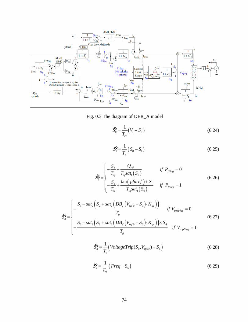
74
Fig. 0.3 The diagram of DER_A model
( )0 0
1t
rv
S V ST
= −& (6.24)
( )1 8 1
1
p
S S ST
= −& (6.25)
( )
( )
( )
2
1 0
2
12
1 0
0
tan1
ref
fFlag
iq iq
fFlag
iq iq
QSif P
T T sat SS
pfaref SSif P
T T sat S
− + =
= +− + =
& (6.26)
( )( )( )
( )( )( )
3 2 2 2 0 0
3
3 2 2 2 0 0 4
0
1
V ref qv
tripFlag
g
V ref qv
tripFlag
g
S sat S sat DB V S Kif V
TS
S sat S sat DB V S K Sif V
T
− + − − =
= − + − − =
& (6.27)
( )4 0 4
1( , )rfrac
v
S VoltageTrip S V ST
= −& (6.28)
( )5 5
1
rf
S Freq ST
= −& (6.29)

75
( ) ( )
6 4 1 5 5 6 5
81 5 5
( ( ) ( ) )ig ref dn F ref up F ref
pg
dn up
p p
S K sat P S sat D DB Freq S sat D DB Freq S
K SS G Freq S G Freq S
T T
= − + − + −
+ + − + − −
&
(6.30)
( )( )7
8 7 6
0 0
1
flag
flag
if FreqS
sat sat S if Freq
==
=
&&
(6.31)
( )8 7 8
1
pord
S S ST
= −& (6.32)
( )
( )
7 89 4 9
1 0
9
7 89 9
1 0
( )11
( )10
tripflag
g
tripflag
g
sat Ssat S S if V
T sat SS
sat Ssat S if V
T sat S
− =
=
− =
& (6.33)
6.4 Order Reduction of WECC Composite Load Model
In this section, we will derive the reduced-order large-signal model of WECC composite load
model using singular perturbation method. For the purpose of order-reduction, we only focus on
the dynamic components. These components are connected in parallel and we will reduce each
individual component's order.
6.4.1 Reduced-Order Three-Phase Motor Model
Each three-phase motor model has five states, , , , , .M q d q dx E E E E SLIP = % When applying the
singular perturbation method, the first step is to identify the slow and fast dynamics. Since the fast
dynamics are characterized by the small perturbation coefficient , we rewrite the left-hand-side
of the dynamic equations as
0 0 0 0, , , , .T
p q p d pp q pp dT E T E T E T E H SLIP
& & & & & (6.34)
Given one set of parameters setting in Table 6.1, equation (6.34) becomes
0.1 ,0.1 ,0.0026 ,0.0026 ,0.1 .T
q d q dE E E E SLIP
& & & & & (6.35)

76
Table 0.1 Parameters of three-phase motor model
Motor A Motor B Motor C
sAr 0.04 sBr 0.03 sCr 0.03
sAL 1.8 sBL 1.8 sCL 1.8
pAL 0.1 pBL 0.16 pCL 0.16
ppAL 0.083 ppBL 0.12 ppCL 0.12
poAT 0.092 poBT 0.1 poCT 0.1
ppoAT 0.002 ppoBT 0.0026 ppoCT 0.0026
AH 0.05 BH 1 CH 0.1
AA 0 BA 0 CA 0
AB 0 BB 0 CB 0
AC 0 BC 0 CC 0
AD 1 BD 1 CD 1
trqAE 0 trqBE 2 trqCE 2
Ap -1 Bp -1 Cp -1
Aq -1 Bq -1 Cq -1
0 A 120π 0B 120π 0C 120π
The smaller perturbation coefficients in equation (6.35) suggest that dynamic response velocities
of , ,q dE E SLIP are much slower than the rest of the states. This difference is also an evidence
of the two-time-scale property of this model. Then the slow and fast dynamics are divided as
follows

77
M
M
M
xx
z
=
& (6.36)
where , ,M q dx E E SLIP = , ,M q dz E E
= . For consistence, define the input voltages ,q dV V
as MU . Following the singular perturbation method (6.1)-(6.5), we can obtain the reduced-order
large-signal model of three-phase motor as
( )1 1 0 0 2 3
0
1M M d s p P M M
p
x x i L L T x xT
= − − − −
& (6.37)
( )2 2 0 0 1 3
0
1M M q s p P M M
p
x x i L L T x xT
= − + − +
& (6.38)
( ) ( )2 1
32
M d M q
M
TL p h x i q h x ix
H
− − =& (6.39)
where the quasi-steady-state solutions are
( ) ( ) ( ) ( ) ( )2
1 1 2 1 22 2
1M p pp s M p pp s M p pp p p pp s
s p
h x L L r x L L r x L L L U L L rUr L
= + − − − − − − +
(6.40)
( ) ( ) ( ) ( ) ( )2
2 1 2 1 22 2
1M p pp s M p pp s M p pp s p pp p
s p
h x L L r x L L r x L L rU L L L Ur L
= − − + + − − − +
(6.41)
the other algebraic equations are derived as
( ) ( ) ( )2
0 3 3 0 31 1 1Etrq
m M M MTL T A x B x C D x = − + − + + −
(6.42)
( ) ( )0 2 1m M d M qT p h x i q h x i= + (6.43)
( ) ( )1 1 2 22 2 2 2
psq M M M M
s p s p
Lri U x U x
r L r L= + − +
+ + (6.44)
( ) ( )1 1 2 22 2 2 2
p sd M M M M
s p s p
L ri U x U x
r L r L= + + +
+ + (6.45)
After obtaining the quasi-steady-state model, we should also derive the boundary-layer model and
check whether the Assumptions 1-3 are satisfied. If satisfied, then we can proceed to approximate
slow and fast states in terms of the solutions of the reduced model and boundary-layer model. If
not, we should make some modification like coordinate transformation or redefining the states,
then reselect the slow and fast states. In this case, it can be verified that the assumptions are

78
satisfied under such parameter setting. Moreover, the small perturbation coefficient satisfies the
condition of equation (6.11). Therefore, the fast states can be approximated by the quasi-steady
state ( )i Mh x only. This approximation significantly simplifies the reduced model.
6.4.2 Reduced-Order DER_A model
The DER_A model has 10 states in total, 0 1 9, , , .Dx S S S= % Different from the three-phase
motor model, due to the existence of switches such as FlagPf and FlagPQ , the DER_A model is
actually a switching system consisting of 62 subsystems. Each subsystem is determined when the
switches are fixed. Since these switches are preset, we only need to derive the reduced-order model
for each subsystem. For brevity, we give the reduced-order model for one of the subsystems to
illustrate the reducing procedure. The reduced models for other subsystems can be obtained using
the same method.
To find the small perturbation coefficient , we rewrite the dynamics a
0 1 2 3 4 5 6 7 8 9, , , , , , , , , .T
rv p iq g v rf p rf pord gT S T S T S T S T S T S T T S S T S T S & & & & & & & & & & (6.46)
Given the parameter setting in Table 6.2, equation (6.46) becomes
0 1 2 3 4 5 6 7 8 90.01 , 0.01 , 0.005 , 0.005 , 0.005 ,0.01 , 0.01 0.01 , , 0.005 , 0.005 .T
S S S S S S S S S S & & & & & & & & & &
The smaller perturbation coefficients in equation (6.47) suggest that dynamic response velocities
of 0 1 5 7, , ,S S S S are much slower than the rest of the states. This difference is also an evidence
of the two-time-scale property of this model. Then the slow and fast dynamics are divided as
follows
.D
D
D
xx
z
=
& (6.47)
where 0 1 5 7, , ,Dx S S S S= , 2 3 4 6 8 9, , , , ,Dz S S S S S S= . Defining the input voltages ,tV Freq as
DU , following the same procedure as above (6.1)-(6.5), we can derive the reduced-order large-
signal model of DER_A as
( )1 1 1
1D D D
rv
x U xT
= −& (6.48)
( )2 4 2
1D D D
p
x x xT
= −& (6.49)

79
( )3 2 3
1D D D
rf
x U xT
= −& (6.50)
4 0Dx =& . (6.51)
Table 0.2 Parameters of DER_A model
Parameters Values Parameters Values
rvT 0.02 s Tpord 0.02 s
pT 0.02 s mindP -0.5 pu/s
iqT 0.02 s maxdP 0.5 pu/s
0refV 0 pu tripflagV 1
qvK 5 pu/pu 1qlI -1 pu
gT 0.02 s 1qhI 1 pu
FlagPf 1 eX 0.25 pu
maxI 1.2 tripflagF 1
dbd1 -99 flagPQ 0
dbd2 99 typeflag 1
vT 0.02 s prV 0.8 pu
loV 0.44 pu upD 0
1lV 0.49 pu emaxf 99 pu
0hV 1.2 pu eminf -99 pu
1hV 1.15 pu 1dbdf -0.0006
0vlt 0.16 s 2dbdf 0.0006

80
1vlt 0.16 s flagFreq 0
0vht 0.16 s minP 0 pu
1vht 0.16 s maxP 1.1 pu
rfracV 0.7 pgK 0.1 pu
rfT 0.02 s igK 10 pu
dnD 20 c 1 s
a 0.8 pu d 0.9 pu
b 5 Base: 12.47 kV and 15.0 MVA
The d - q axis currents di and qi are states 3S ( 2Dz ) and 9S ( 6Dz ), respectively. Their equations
are
( )2 1 2ˆ( ) ,q D D rfrac Di sat x VP x V y= + (6.52)
( )( )7 4
9 1 6
1 1
( )ˆ,D
d D rfrac D
D
sat xi sat VP x V y
sat x
= +
(6.53)
( )
( )( )2
3 0 1
1 1
tan( )
D
D qv V ref D
D
pfaref xx K sat DB V x
sat x = + −
(6.54)
where 2ˆ
Dy and 6ˆ
Dy are the solutions of boundary-layer model:
1 1D Dy y= −& (6.55)
( ) 2 3 2 1 2 2 1, ( ) ( )D D D D rfrac D D Dy y y VP x V sat x sat y x = − − + +& (6.56)
3 3D Dy y= −& (6.57)
4 5D rf Dy T y= −& (6.58)
5 5D Dy y= −& (6.59)
( )( )
( )( )7 4 7 5 4
6 6 9 1 9 3 1
1 1 1 1
( ) ( ), ,D D D
D D D rfrac D D rfrac
D D
sat x sat y xy y sat VP x V sat y VP x V
sat x sat x
+ = − − + +
& (6.60)

81
As mentioned above, only if the assumptions are satisfied, we can use the reduced model to
estimate the original model. It can be verified that the assumptions 1-3 are satisfied in this case.
However, the condition of equation (6.11) is not guaranteed. Therefore, we should add a
complementary term ˆ( / )y t which is the solution of boundary-layer model.
The two-time-scale property makes the load model a stiff ordinary differential equation problem.
A problem is stiff if the solution being searched varies slowly, however there are nearby solutions
varying rapidly. Therefore, the numerical method must take small steps to obtain satisfactory
results. The stiffness can increase the computational time. The application of singular perturbation
method reduces the order as well as convert the load model from a stiff problem to a non-stiff one,
thus reducing the computational time from both sides and allowing the use of non-stiff solver.
6.5 Model Validation via Simulation
In this section, the reduced-order model derived in this chapter is verified through simulation. The
reduced-order models of three-phase motor and DER_A are tested on Matlab using different
solvers. We compare the performance of the reduced model with the original model to verify the
effectiveness of the reduced model. Moreover, we compare the computational time between the
two models and different solvers to show the efficiency of reducing computational burden.
6.5.1 Validation of Reduced-Order Three-Phase Motors
To verify the proposed reduced-order model of three-phase motor, we simulated the reduced and
original model in Matlab with the same input voltage. Consequently, we can compare their output
power and other states. Refer to [107], the bus voltage input is generated by (6.61). The parameters
are set as shown in Table 6.2.
( )
( )
( )
1 1 / 60
(1 )( 1 )1 1 / 60 1
/ 60
1
a if t b
d c tV t if b t c
b c
otherwise
+
− + −= + + +
−
„
„ (6.61)
Fig. 6.4 shows the generated input voltage. As shown in Fig. 6.5, 6.6 and 6.7 are the state response
qE and dE of motor A, motor B and motor C, respectively. The blue solid line denotes the qE
and dE of original model, while the red dashed line represents that of reduced-order model. Fig.
6.8, 6.9 and 6.10 shows the output real and reactive power. The blue solid line denotes the real and
reactive power of original model, while the red dashed line represents that of reduced-order model.
The mean squared errors of real and reactive power between the original and reduced model are
shown in Table. 6.3. The small errors show the accuracy of the proposed reduced-order three-
phase model. Moreover, if using ODE45, which is a non-stiff ODE solver, the computational time
of the original and reduced model are 8.8120 s and 0.1926 s, respectively. If using ODE15s, which
is a stiff ODE solver, the computational time of the original and reduced model are 1.0975 s and
0.1785 s, respectively. This comparison shows that the singular perturbation method converts the
original high-order stiff problem to a reduced-order non-stiff problem while reducing the

82
computational time remarkably. This reduction will be more significant in large-scale system with
multiple composite loads.
Table 0.3 The mean squared errors between original and reduced-order model of three-phase
motor
Motor
Power
Mean square error (MSE)
Motor A Motor B Motor C
Real power 41.0509 10− 41.1295 10−
58.0264 10−
Reactive power 51.1422 10− 51.4294 10−
52.1112 10−
Fig. 0.4 Bus voltages of reduced and original model of three-phase motors

83
Fig. 0.5 Parameters of reduced and original model of three-phase motor A
Fig. 0.6 Parameters of reduced and original model of three-phase motor B

84
Fig. 0.7 Parameters of reduced and original model of three-phase motor C
Fig. 0.8 Real and reactive power of reduced and original model of three-phase motor A

85
Fig. 0.9 Real and reactive power of reduced and original model of three-phase motor B
Fig. 0.10 Real and reactive power of reduced and original model of three-phase motor C

86
6.5.2 Validation of DER_A model
Similar to the verification process of three-phase motor, we simulated the reduced and original
model of DER_A in Matlab. The voltage input is the same as (6.61). The frequency input is set to
be 60 Hz. The parameters are set as shown in Table 6.2.
Fig. 6.11 shows the filtered voltage and frequency inputs of DER_A. Fig. 6.12 shows the dynamic
power responses of DER_A. The blue solid line denotes the power output of original model, while
the red dashed line represents that of reduced one. Fig. 6.13 shows filtered voltage tfiltV , filtered
generated power genfiltP , and filtered current qi and di of reduced and original model of DER_A.
The mean square errors (MSE) of real and reactive power are 47.1363 10− and
51.3045 10− ,
respectively. Furthermore, the computational time of the original and reduced model using ODE45
are 11.205 s and 0.2074 s, respectively; the computational time of the original and reduced model
using ODE15s are 2.0012 s and 0.1598 s, respectively.
Fig. 0.11 Filtered input voltages and frequency of original and reduced model of DER_A

87
Fig. 0.12 Real and reactive power of reduced and original model of DER_A
Fig. 0.13 Filtered voltage, filtered generated power, and filtered current of reduced and original
model of DER_A

88
6.6 Summary
This work developed the reduced-order large-signal model of WECC CMPLDW + DER_A model.
Several simulations are conducted in Matlab. The comparison analysis shows the accuracy of the
proposed reduced model. It also shows that the computational time is reduced significantly using
reduced model.

89
7. Conclusion and Future Work
In this report, we first reviewed the state-of-the-art of load models and parameter identification
methods. Second, a cutting-edge parameter reduction approach based on active subspace is
proposed to deal with the high dimensional parameter space of the WECC composite load model,
which is more comprehensive but with large number of parameters. Third, we proposed a novel
deep reinforcement learning based parameter identification for the WECC composite load model.
Then, we also test the real PMU data from utility on Python and PSSE using the salp swarm
algorithm. Finally, we also proposed the large-signal order reduction method for WECC composite
load model which is able to reduce the computational time of each call of the WECC composite
load model.
The future research directions are suggested in terms of modeling and identification technologies:
For load model structure development, more sophisticated models that balance flexibility and
complexity are needed. Load consumption is time varying due to human behaviors and weather
conditions; thus, different load models may be found in different time periods. Conventional load
modeling methods using measurement data in a certain period may not be able to capture time-
varying load behaviors, and lack generalizability. More research is needed to develop advanced
algorithms to perform online load modeling using the real-time data. After developing new load
models, they should be integrated in power system analysis programs. How to model and represent
seasonal and geographical variations in load models and load composition is also an ongoing
research topic. Capturing the time-varying nature of load behaviors is useful to voltage control,
state estimation, and energy management. The increasing penetration of DGs and the
implementation of demand-side management poses additional challenges to load modeling.
WECC identified DGs as one of the main priorities in their further efforts to update CLM. DGs
and power electronic loads may have complex control systems, which need to be taken into account
in the model development. Customer behavior-driven and DR-enabled load models need to be
built to facilitate DR studies. Distribution system models were not well studied in the past. There
is a need to develop novel models with reduced complexity and computational requirements to
represent ADNs and MGs. Modeling and aggregating DGs, controllable loads, and other
technologies in ADNs and MGs is a major research topic. New loads such as electric vehicles and
storage devices should be modeled to accurately represent the system. Moreover, modeling the
interface and control logics of power electronics and testing their impact on stability and dynamic
studies is an important research topic.
Future research on parameter estimation algorithms should be able to process data from existing
and emerging measurement devices with different resolutions, such as smart meters, PMUs, and
SCADA. Meanwhile, the algorithms should be robust to bad data, missing measurements, changes
in the voltage regulation scheme, and noises.

90
References
[1] C. W. Taylor, Power system voltage stability, McGraw-Hill, 1994.
[2] P. Kundur, Power system stability and control, EPRI series, New York: McGraw-Hill,
1994.
[3] K. E. Wong, M. E. Haque and M. Davies, “Component-based dynamic load modeling of
a paper mill,” in Proc. 2012 22nd Australasian Universities Power Eng. Conf., Bali, 2012,
pp. 1-6.
[4] I. Dzafic, M. Glavic and S. Tesnjak, “A component-based power system model-driven
architecture,” IEEE Trans. Power Syst., vol. 19, no. 4, pp. 2109-2110, Nov. 2004.
[5] D. Kosterev, A. Meklin, J. Undrill, B. Lesieutre, W. Price, D. Chassin, R. Bravo and S.
Yang, “Load modeling in power system studies: WECC progress update,” in Proc. IEEE
PES General Meeting, Pittsbugh, PA, 2008,pp. 1-8.
[6] WECC MVWG Load Model Report ver. 1.0 (June 2012). [Online]
Available:https://www.wecc.biz/Reliability/WECC%20MVWG%20Load%20Model%2
0Reprt%20ver%201%200.pdf
[7] Electrical Power Research Institute (EPRI), “Advanced load modeling,” Tech. Rep.
1007318, Sept. 2002.
[8] A. Gaikwad, P. Markham and P. Pourbeik, “Implementation of the WECC Composite
Load Model for utilities using the component-based modeling approach,’’ in Proc
IEEE/PES Transmission and Distribution Conf. and Expo., Dallas, TX, 2016, pp. 1-5.
[9] L. Zhu, X. Li, H. Ouyang, Y. Wang, W. Liu and K. Shao, “Research on component-based
approach load modeling based on energy management system and load control system,”
in Proc. IEEE PES Innovative Smart Grid Technologies, Tianjin, 2012, pp. 1-6.
[10] S. -H. Lee, S. -E. Son, S. -M. Lee, “Kalman-filter based static load modeling of real power
system using K-EMS data,” J. Elect. Eng. Technol, vol. 7, no. 3, pp. 304-311, June 2012.
[11] H. Renmu, Ma Jin and D. J. Hill, “Composite load modeling via measurement approach,”
IEEE Trans. Power Syst., vol. 21, no. 2, pp. 663¬672, May 2006.
[12] Byoung-Kon Choi et al., “Measurement-based dynamic load models: derivation,
comparison, and validation,” IEEE Trans. Power Syst., vol. 21, no. 3, pp. 1273-1283,
Aug. 2006.
[13] Electrical Power Research Institute (EPRI), “Measurement-Based Load Modeling,”
Tech. Rep. 1014402, Sept. 2006.
[14] J. Ma, D. Han, R. M. He, Z. Y. Dong and D. J. Hill, “Reducing identified parameters of
measurement-based composite load model,” IEEE Trans. Power Syst., vol. 23, no. 1, pp.
73-83, Feb. 2008.
[15] Ma Jin, H. Renmu and D. J. Hill, “Load modeling by finding support vectors of load data
from field measurements,” IEEE Trans. Power Syst., vol. 21, no. 2, pp. 723-735, May
2006.

91
[16] I. F. Visconti, D. A. Lima, J. M. C. d. S. Costa and N. Sobrinho, “Measurement-based
load modeling using transfer functions for dynamic simulations,” IEEE Trans. Power
Syst., vol. 29, no. 1, pp. 111-120, Jan. 2014.
[17] D. Han, J. Ma, R. m. He and Z. Y. Dong, “A real application of measurement-based load
modeling in large-scale power grids and its validation,” IEEE Trans. Power Syst., vol.
24, no. 4, pp. 1753-1764, Nov.2009.
[18] B. K. Choi and H. D. Chiang, “Multiple solutions and plateau phenomenon in
measurement-based load model development: issues and suggestions,” IEEE Trans.
Power Syst., vol. 24, no. 2, pp. 824-831, May 2009.
[19] F. Hu, K. Sun, A. Del Rosso, E. Farantatos and N. Bhatt, “Measurement based real-time
voltage stability monitoring for load areas, ^ IEEE Trans. Power Syst., vol. 31, no. 4, pp.
2787-2798, July 2016.
[20] H. Bai, P. Zhang and V. Ajjarapu, “A novel parameter identification approach via hybrid
learning for aggregate load modeling,” IEEE Trans. Power Syst., vol. 24, no. 3, pp. 1145-
1154, Aug. 2009.
[21] Y. Ge, A. J. Flueck, D. K. Kim, J. B. Ahn, J. D. Lee and D. Y. Kwon, “An event-oriented
method for online load modeling based on synchrophasor data,” IEEE Trans. Smart Grid,
vol. 6, no. 4, pp. 2060-2068, July 2015.
[22] P. Regulski, D. S. Vilchis-Rodriguez, S. Djurovic and V. Terzija, “Estimation of
composite load model parameters using an improved particle swarm optimization
method,” IEEE Trans. Power Del., vol. 30, no. 2, pp. 553-560, April 2015.
[23] J. K. Kim et al., “Fast and reliable estimation of composite load model parameters using
analytical similarity of parameter sensitivity,” IEEE Trans. Power Syst., vol. 31, no. 1,
pp. 663-671, Jan. 2016.
[24] X. Zhang, S. Grijalva and M. J. Reno, “A time-variant load model based on smart meter
data mining,” in Proc. IEEE PES General Meeting Conf. and Expo., National Harbor,
MD, 2014, pp. 1-5.
[25] B. Y. Ku, R.J. Thomas, C.-Y. Chiou, C.-J. Lin, “Power system dynamic load modeling
using artificial neural networks,” IEEE Trans. Power Syst., vol. 9, no. 4, pp. 1868-1874,
Nov. 1994.
[26] A. Keyhani, W. Lu, G.T. Heydt, “Composite neural network load models for power
system stability analysis,” in Proc. IEEE PES Power Syst. Conf. and Expo., 2004, pp.
1159-1163.
[27] M. Bostanci, J. Koplowitz, C.W. Taylor, “Identification of power system load dynamics
using artificial neural networks, IEEE Trans. Power Syst., vol.12, no.4, pp.1468-1473,
Nov. 1997.
[28] G. W. Chang, C. I. Chen and Y. J. Liu, “A neural-network-based method of modeling
electric arc furnace load for power engineering study,” IEEE Trans. Power Syst., vol. 25,
no. 1, pp. 138-146, Feb. 2010.

92
[29] Dingguo Chen and R. R. Mohler, “Neural-network-based load modeling and its use in
voltage stability analysis,” IEEE Trans. on Control Syst. Tech., vol. 11, no. 4, pp. 460-
470, July 2003.
[30] T. Hiyama, M. Tokieda, W. Hubbi and H. Andou, “Artificial neural network based
dynamic load modeling,^ IEEE Trans. Power Syst., vol. 12, no. 4, pp. 1573-1583, Nov.
1997.
[31] IEEE Task Force on Load Representation for Dynamic Performance, “Load
representation for dynamic performance analysis (of power systems),” IEEE Trans.
Power Syst., vol. 8, no. 2, pp. 472-482, May 1993.
[32] IEEE Task Force on Load Representation for Dynamic Performance, “Standard load
models for power flow and dynamic performance simulation,” IEEE Trans. Power Syst.,
vol. 10, pp. 1302-1313, 1995.
[33] IEEE Task Force on Load Representation for Dynamic Performance, “Bibliography on
load models for power flow and dynamic performance simulation,” IEEE Trans. Power
Syst., vol. 10, no. 1, pp. 523-538, Feb. 1995.
[34] J. V. Milanovic, K. Yamashita, S. Villanueva, S. Djokic and L. M. Korunovic,
“International industry practice on power system load for modeling,” IEEE Trans. Power
Syst., vol. 28, no. 3, pp. 3038-3046, Aug. 2013.
[35] J. V. Milanovic, et al., “CIGRE WG C4.605: Modelling and aggregation of loads in
flexible power networks,” 2014.
[36] A. J. Collin, G. Tsagarakis, A. E. Kiprakis and S. McLaughlin, “Development of low-
voltage load models for the residential load sector,” IEEE Trans. Power Syst., vol. 29,
no. 5, pp. 2180-2188, Sept. 2014.
[37] S. M. Zali and J. V. Milanovic, “Generic model of active distribution network for large
power system stability studies,” IEEE Trans. Power Syst., vol. 28, no. 3, pp. 3123-3133,
Aug. 2013.
[38] J. V. Milanovic and S. Mat Zali, “Validation of equivalent dynamic model of active
distribution network cell,” IEEE Trans. Power Syst., vol. 28, no.3,pp. 2101-2110, Aug.
2013.
[39] Kuo-Hsiung Tseng, Wen-Shiow Kao and Jia-Renn Lin, “Load model effects on distance
relay settings,” IEEE Trans. Po'wer Del., vol. 18, no.4, pp. 1140-1146, Oct. 2003.
[40] W.W. Price, K.A. Wirgau, A. Murdoch, F. Nozari, “Load modeling for power flow and
transient stability studies,” EPRI Report EL-5003, Project 849-7, 1987.
[41] EPRI, “Extended transient-midterm stability program package FACTS version user’s
manual,” EPRI Project 1208-9, September 1990.
[42] P. Jazayeri, W. Rosehart and D. T. Westwick, “A multistage algorithm for identification
of nonlinear aggregate power system loads,” IEEE Trans. Power Syst., vol. 22, no. 3, pp.
1072-1079, Aug. 2007.
[43] D. Hill, “Nonlinear dynamic load models with recovery for voltage stability studies,”
IEEE Trans. Power Syst., vol. 8, no. 1, pp. 163-176, Feb.1993.

93
[44] D. Karlsson, D.J. Hill, “Modeling and identification of nonlinear dynamic loads in power
systems,” IEEE Trans. Power Syst., vol.9, no.1, pp.157¬166, Feb 1994.
[45] W. Xu and Y. Mansour, “Voltage stability analysis using generic dynamic load models,”
IEEE Trans. Power Syst., vol. 9, no. 1, pp. 479-493, Feb. 1994.
[46] W. S. Kao, C. J. Lin, C. T. Huang, Y. T. Chen, and C. Y. Chiou, “Comparison of
simulated power system dynamics applying various load models with actual recorded
data,” IEEE Trans. Power Syst., vol. 9, no. 1, pp. 248-254, Feb. 1994.
[47] W. S. Kao, “The effect of load models on unstable low-frequency oscillation damping in
Taipower system experience w/wo power system stabilizers,” IEEE Trans. Power Syst.,
vol. 16, no. 3, pp. 463-472, Aug. 2001.
[48] D. N. Kosterev, C. W. Taylor and W. A. Mittelstadt, “Model validation for the August
10 1996 WSCC system outage,” IEEE Trans. Power Syst., vol. 14, pp. 967-979, Aug.
1999.
[49] L. Pereira, D. Kosterev, P. Mackin, D. Davies, J. Undrill and W. Zhu, “An interim
dynamic induction motor model for stability studies in the WSCC,” IEEE Trans. Power
Syst., vol. 17, no. 4, pp. 1108-1115, Nov. 2002.
[50] B. Williams, W. Schmus, D. Dawson, “Transmission voltage recovery delayed by stalled
air conditioner compressors,” IEEE Trans. Power Syst., vol.7, no.3, pp.1173-1181, Aug.
1992.
[51] J. Shaffer, “Air conditioner response to transmission faults,” IEEE Trans. Power Syst.,
vol.12, no.2, pp.614-621, May 1997.
[52] A. Bokhari, et al., “Experimental determination of ZIP coefficients for modern
residential, commercial and industrial loads,” IEEE Trans. Power Del., vol. 29, no. 3, pp.
1372-1381, Oct. 2013.
[53] L. M. Hajagos and B. Danai, “Laboratory measurements and models of modern loads and
their effect on voltage stability studies,” IEEE Trans. Power Syst., vol. 13, no. 2, pp. 584-
592, May 1998.
[54] N. Lu, Y. Xie, Z. Huang, F. Puyleart, and S. Yang, “Load component database of
household appliances and small office equipment,” in Proc. IEEEPES Gen. Meeting,
Pittsburgh, PA, 2008, pp. 1-5.
[55] X. Liang, “A new composite load model structure for industrial facilities,” IEEE Trans.
on Ind. Appl., to be published.
[56] X. Liang, and W. Xu, “Aggregation method for motor drive systems,” Electric Power
Systems Research (Elsevier), vol. 117, pp. 27 - 35, Dec. 2014.
[57] Q. S. Liu, Y. P. Chen, D. F. Duan, “The load modeling and parameter identification for
voltage stability analysis,” in Proc. Int. Conf. Power Syst. Technol., 2002, pp. 2030-2033.
[58] I. Hiskens, “Nonlinear dynamic model evaluation from disturbance measurements,”
IEEE Trans. Power Syst., vol. 16, no. 4, pp. 702-710, Nov. 2001.

94
[59] S. Z. Zhu, J. H. Zheng, S. D. Shen, G. M. Luo, “Effect of load modeling on voltage
stability,” in Proc. IEEE Power Eng. Soc. Summer Meeting, Seattle, WA, 2000, pp. 395
- 400.
[60] S. Kamoun and R. P. Malham6, “Convergence characteristics of a maximum likelihood
load model identification scheme,” Automatica, vol. 28, no. 5, pp. 885-896, Sept. 1992.
[61] V. Knyazkin, C. Caizares, and L. Sder, “On the parameter estimation and modeling of
aggregate power system loads,” IEEE Trans. Power Syst., vol. 19, no. 2, pp. 1023-1031,
May 2004.
[62] S.-H. Lee, S.-E. Son, S.-M. Lee, J.-M. Cho, K.-B. Song, and J.-W. Park, “Kalman-filter
based static load modeling of real power system using K EMS data,” J. Elect. Eng.
Technol., vol. 7, no. 3, pp. 742-750, May 2012.
[63] J. Ma, Z.Y. Dong, P. Zhang, “Using a support vector machine (SVM) to improve
generalization ability of load model parameters,” in Proc. IEEE PES Power Syst. Con/
and Expo., Seattle, WA, 2009, pp. 1-8.
[64] L. T. M. Mota, A. A. Mota, “Load modeling at electric power distribution substations
using dynamic load parameters estimation,” Int. J. Elect. Power Energy Syst., vol. 26, no.
10, pp. 805-811, 2004.
[65] Z. Wang and J. Wang, "Time-Varying Stochastic Assessment of Conservation Voltage
Reduction Based on Load Modeling," IEEE Trans. On Power Syst., vol. 29, no. 5, pp.
2321-2328, Sep. 2014
[66] A. Rouhani and A. Abur, “Real-time dynamic parameter estimation for an exponential
dynamic load model,” IEEE Trans. Smart Grid, vol. 7, no. 3, pp. 1530-1536, May 2016.
[67] E. A. Wan and R. Van der Merwe, “The unscented Kalman filter,” Kalman Filtering and
Neural Networks, Wiley, 2001.
[68] Z. Wang and J. Wang, "Review on implementation and assessment of conservation
voltage reduction," IEEE Trans. Power Syst., vol. 29, no. 3, pp. 1303-1315, May 2014.
[69] J. Zhao, Z. Wang, and J. Wang, "Robust time-varying load modeling for conservation
voltage reduction assessment," IEEE Trans. Smart Grid, accepted for publication.
[70] Vignesh V, S. Chakrabarti and S. C. Srivastava, “Classification and modelling of loads
in power systems using SVM and optimization approach,” in Proc. IEEE PES General
Meeting, Denver, CO, 2015, pp. 1-5.
[71] G. Golub and V. Pereyra, “Separable nonlinear least squares: the variable projection
method and its applications,” Inverse Problems, vol. 19, no. 2, Feb. 2003.
[72] A. Patel, K. Wedeward, and M. Smith, “Parameter estimation for inventory of load
models in electric power systems,” in Proc. The World Congress on Eng. and Comp. Sci.,
San Francisco, USA, 2014, pp. 233¬238.
[73] S. Sonet al., “Improvement of composite load modeling based on parameter sensitivity
and dependency analyses,” IEEE Trans. Power Syst., vol. 29, no. 1, pp. 242-250, Jan.
2014.

95
[74] J. K. Kim et al., “Fast and reliable estimation of composite load model parameters using
analytical similarity of parameter sensitivity,” IEEE Trans. Power Syst., vol. 31, no. 1,
pp. 663-671, Jan. 2016.
[75] Z. Wang and J. Wang, "Analysis of performance and efficiency of conservation voltage
optimization considering load model uncertainty," J. of Energy Eng.,
10.1061/(ASCE)EY.1943-7897.0000190, 2014.
[76] Z. Wang, J. Wang, B. Chen, M. Begovic, and Y. He, "MPC-based voltage/var
optimization for distribution circuits with distributed generators and exponential load
models," IEEE Trans. Smart Grid, vol. 5, no. 5, pp. 2412-2420, Sep. 2014.
[77] Z. Wang and Y. He, "Two-stage optimal demand response with battery energy storage
systems," IET Generation, Transmission & Distribution, vol. 10, no. 5, pp. 1283-1293,
Apr. 2016.
[78] Electrical Power Research Institute (EPRI), “End-use load composition estimation using
smart meter data,” Tech. Rep. 1020060, Dec. 2010.
[79] J. Zhao, G. Zhang, M. La Scala, and Z. Wang, “Enhanced robustness of state estimator
to bad data processing through multi-innovation analysis,” IEEE Trans. on Ind.
Informatics, accepted for publication.
[80] J. Zhao, Z. Wang, C. Chen, and G. Zhang, "Robust voltage instability predictor," IEEE
Trans. Power Syst., vol. 11, no. 2, pp. 401-408, Jan. 2017
[81] K. Zhang, H. Zhu, and S. Guo, “Dependency analysis and improved parameter estimation
for dynamic composite load modeling,” IEEE Trans. Power Syst., vol. 32, no. 4, pp.
3287–3297, Jul. 2017.
[82] C. Wang, Z. Wang, J. Wang, and D. Zhao, “Robust Time-Varying Parameter
Identification for Composite Load Modeling,” IEEE Trans. Smart Grid, vol. 10, no. 1,
pp. 967–979, Jan. 2019.
[83] A. Arif, Z. Wang, J. Wang, B. Mather, H. Bashualdo, and D. Zhao,“Load Modeling-A
Review,” IEEE Trans. Smart Grid, vol. 9, no. 6, pp. 5986–5999, Nov. 2018.
[84] Z. Ma, Z. Wang, D. Zhao, and B. Cui, “High-fidelity large-signal order reduction
approach for composite load model,” IET Gener. Transm. Distrib., vol. 14, no. 21, pp.
4888–4897, Aug. 2020.
[85] Q. Huang, R. Huang, B. J. Palmer, Y. Liu, S. Jin, R. Diao, Y. Chen, and Y. Zhang, “A
generic modeling and development approach for WECC composite load model,” Electr.
Power Syst. Res., vol. 172, pp. 1–10, Jul. 2019.
[86] A. Saltelli, “Sensitivity analysis for importance assessment,” Risk Anal., vol. 22, no. 3,
pp. 579–590, Jun. 2002.
[87] T. Homma and A. Saltelli, “Importance measures in global sensitivity analysis of
nonlinear models,” Reliab. Eng. Syst. Saf., vol. 52, no. 1, pp. 1–17, Apr. 1996.
[88] S. Marino, I. B. Hogue, C. J. Ray, and D. E. Kirschner, “A methodology for performing
global uncertainty and sensitivity analysis in systems biology,” J. Theor. Biol., vol. 254,
no. 1, pp. 178 – 196, Sep. 2008.

96
[89] M. D. Morris, “Factorial sampling plans for preliminary computational experiments,”
Technometrics, vol. 33, no. 2, pp. 161–174, May 1991.
[90] D. K. Lin, “A new class of supersaturated designs,” Technometrics, vol. 35, no. 1, pp.
28–31, Feb. 1993.
[91] A. Dean and S. Lewis, Screening: methods for experimentation in industry, drug
discovery, and genetics. Springer Science & Business Media, 2006.
[92] B. Bettonvil and J. P. Kleijnen, “Searching for important factors in simulation models
with many factors: Sequential bifurcation,” Eur. J. Oper. Res., vol. 96, no. 1, pp. 180–
194, Jan. 1997.
[93] K. Hinkelmann and O. Kempthorne, Design and analysis of experiments. Wiley Online
Library, 1994, vol. 1.
[94] B. Iooss and P. Lemaıtre, “A review on global sensitivity analysis methods,” in
Uncertainty management in simulation-optimization of complex systems. Springer,
2015, pp. 101–122.
[95] I. M. Sobol, “Global sensitivity indices for nonlinear mathematical models and their
monte carlo estimates,” Math. Comput. Simul., vol. 55, no. 1-3, pp. 271–280, Feb. 2001.
[96] A. Saltelli, P. Annoni, I. Azzini, F. Campolongo, M. Ratto, and S. Tarantola,“Variance
based sensitivity analysis of model output. design and estimator for the total sensitivity
index,” Comput. Phys. Commun., vol. 181, no. 2, pp. 259–270, Feb. 2010.
[97] A. Saltelli, M. Ratto, T. Andres, F. Campolongo, J. Cariboni, D. Gatelli, M. Saisana, and
S. Tarantola, Global sensitivity analysis: the primer. John Wiley & Sons, 2008.
[98] A. Saltelli and P. Annoni, “How to avoid a perfunctory sensitivity analysis,” Environ.
Model. Softw., vol. 25, no. 12, pp. 1508–1517, Dec. 2010.
[99] H. Scheffe, The analysis of variance. John Wiley & Sons, 1999.
[100] A. Saltelli and R. Bolado, “An alternative way to compute fourier amplitude sensitivity
test (FAST),” Compu. Stat. Data An., vol. 26, no. 4, pp. 445 – 460, Feb. 1998.
[101] F. Bu, Z. Ma, Y. Yuan, and Z. Wang, “WECC composite load model parameter
identification using evolutionary deep reinforcement learning,” IEEE Trans. Smart Grid,
vol. 11, no. 6, pp. 5407–5417, Jul. 2020.
[102] J.-Y. Tissot and C. Prieur, “Bias correction for the estimation of sensitivity indices based
on random balance designs,” Reliab. Eng. Syst. Safe., vol. 107, pp. 205 – 213, Nov. 2012.
[103] J. Ma, D. Han, R.-M. He, Z.-Y. Dong, and D. J. Hill, “Reducing identified parameters of
measurement-based composite load model,” IEEE Trans. Power Syst., vol. 23, no. 1, pp.
76–83, Jan. 2008.
[104] P. G. Constantine, Active subspaces: Emerging ideas for dimension reduction in
parameter studies. SIAM-Society for Industrial and Applied Mathematics, 2015.
[105] T. Loudon and S. Pankavich, “Mathematical analysis and dynamic active subspaces for
a long term model of HIV,” Math Biosci Eng, vol. 14, no. 3, pp. 709–733, Jun. 2016.

97
[106] P. Constantine, M. Emory, J. Larsson, and G. Iaccarino, “Exploiting active subspaces to
quantify uncertainty in the numerical simulation of the hyshot ii scramjet,” J. Comput.
Phys., vol. 302, pp. 1 – 20, Dec. 2015.
[107] “The new aggregated distributed energy resources (DER A) model for transmission
planning studies: 2019 update,” Electrical Power Research Institute (EPRI), Tech. Rep.,
2019.
[108] “Technical reference document: dynamic load modeling,” North American Reliability
Cooperation, Tech. Rep., 2016.
[109] T. M. Russi, “Uncertainty quantification with experimental data and complex system
models,” Ph.D. dissertation, UC Berkeley, 2010.
[110] Z. Ma, Z. Wang, Y. Wang, R. Diao, and D. Shi, “Mathematical representation of the
WECC composite load model,” J. Modern Power Syst. Clean Energy, vol. 8, no. 5, pp.
1015–1023, Aug. 2019.
[111] R. Huang et al., “Calibrating parameters of power system stability models using advanced
ensemble Kalman filter,” IEEE Trans. Power Syst., vol. 33, no. 3, pp. 2895–2905, Oct.
2017.
[112] Y. Zhang, J. Wang, and Z. Li, “Uncertainty modeling of distributed energy resources:
Techniques and challenges,” Curr. Sustain. Energy Rep., vol. 6, no. 2, pp. 42–51, Jun.
2019.
[113] M. Cui, J. Wang, and B. Chen, “Flexible machine learning-based cyberattack detection
using spatiotemporal patterns for distribution systems,” IEEE Trans. Smart Grid, vol. 11,
no. 2, pp. 1805–1808, Mar. 2020.
[114] M. Cui, J. Wang, Y. Wang, R. Diao, and D. Shi, “Robust time-varying synthesis load
modeling in distribution networks considering voltage disturbances,” IEEE Trans. Power
Syst., vol. 34, no. 6, pp. 4438–4450, Nov. 2019.
[115] M. Cui, M. Khodayar, C. Chen, X.Wang, Y. Zhang, and M. E. Khodayar,“Deep learning
based time varying parameter identification for systemwide load modeling,” IEEE Trans.
Smart Grid, vol. 10, no. 6, pp. 6102–6114, Nov. 2018.
[116] J.-K. Kim, K. An, and J. Ma, “Fast and reliable estimation of composite load model
parameters using analytical similarity of parameter sensitivity,” IEEE Trans. Power Syst.,
vol. 31, no. 1, pp. 663–671, Jan. 2016.
[117] S. Son et al., “Improvement of composite load modeling based on parameter sensitivity
and dependency analyses,” IEEE Trans. Power Syst., vol. 29, no. 1, pp. 242–250, Jan.
2014.
[118] U.S. Energy Information Administration. (2011). Share of Energy Used by Appliances
and Consumer Electronics Increases in U.S. Homes. [Online]. Available:
https://www.eia.gov/consumption/residential/reports/2009/electronics.php
[119] U.S. Energy Information Administration. (2018). EIA Electricity Data Now Include
Estimated Small-Scale Solar PV Capacity and Generation. [Online]. Available:
https://www.eia.gov/todayinenergy/detail.php?id=23972

98
[120] J. Zhang, M. Cui, and Y. He, “Robustness and adaptability analysis for equivalent model
of doubly fed induction generator wind farm using measured data,” Appl. Energy, vol.
261, pp. 1–12, Mar. 2020.
[121] WECC Composite Load Model Specifications. Accessed: Jan. 27, 2015. [Online].
Available: http://home.engineering.iastate.edu/∼jdm/ee554/
WECC%20Composite%20Load%20Model%20Specifications%2001-27-2015.pdf
[122] X. Wang, Y. Wang, D. Shi, J. Wang, and Z. Wang, “Two-stage WECC composite load
modeling: A double deep Q-learning networks approach,” IEEE Trans. Smart Grid, early
access, Apr. 15, 2020, doi: 10.1109/TSG.2020.2988171.
[123] E. Conti, V. Madhavan, F. P. Such, J. Lehman, K. Stanley, and J. Clune, “Improving
exploration in evolution strategies for deep reinforcement learning via a population of
novelty-seeking agents,” in Proc. Adv. Neural Inf. Process. Syst., Dec. 2018, pp. 5032–
5043
[124] D. Wierstra, T. Schaul, T. Glasmachers, Y. Sun, J. Peters, and J. Schmidhuber, “Natural
evolution strategies,” J. Mach. Learn. Res., vol. 15, no. 1, pp. 949–980, Mar. 2014.
[125] M. Yamada, W. Jitkrittum, L. Sigal, E. P. Xing, and M. Sugiyama. (2019). High-
Dimensional Feature Selection by Feature-Wise Kernelized Lasso. [Online]. Available:
https://arxiv.org/abs/1202.0515.
[126] S. Wang et al., “A data-driven multi-agent autonomous voltage control framework using
deep reinforcement learning,” IEEE Trans. Power Syst., early access, Apr. 23, 2020, doi:
10.1109/TPWRS.2020.2990179.
[127] W. Kersting, Distribution System Modeling and Analysis. New York, NY, USA: CRC
Press, 2011.
[128] J. D. Glover, M. S. Sarma, and T. J. Overbye, Power System Analysis and Design, 5th
ed. Stamford, CT, USA: Cengage Learn., 2011.
[129] A. Hughes and B. Drury, Electric Motors and Drives, 4th ed. Amsterdam, The
Netherlands: Elsevier, 2013.
[130] H. Wu and I. Dobson, “Analysis of induction motor cascading stall in a simple system
based on the cascade model,” IEEE Trans. Power Syst., vol. 28, no. 3, pp. 3184–3193,
Aug. 2013.
[131] D. C. Yu, H. Liu, H. Sun, S. Lu, and C. Mccarthy, “Protective device coordination
enhancement for motor starting programs,” IEEE Trans Power Del., vol. 20, no. 1, pp.
535–537, Jan. 2005.
[132] A. B. Birchfield, T. Xu, K. M. Gegner, K. S. Shetye, and T. J. Overbye, “Grid structural
characteristics as validation criteria for synthetic networks,” IEEE Trans. Power Syst.,
vol. 32, no. 4, pp. 3258–3265, Jul. 2017.
[133] C. M. Bishop, Pattern Recognition and Machine Learning. New York, NY, USA:
Springer, 2009.
[134] R. D. Quint. (2015). A Look Into Load Modeling: The Composite Load Model. [Online].
Available: https://gig.lbl.gov/sites/all/files/6bquint-composite-load-model-data.pdf

99
[135] “Reliability guide: Parameterization of the DER_A model,” North Amer. Elect. Rel.
Corporat., Atlanta, GA, USA, Rep., 2019.
[136] R. Abbassi, A. Abbassi, A. A. Heidari, and S. Mirjalili, “An efficient SALP swarm-
inspired algorithm for parameters identification of photovoltaic cell models,” Energy
Convers. Manag., vol. 179, pp. 362–372, Jan. 2019.
[137] V. François-Lavet, P. Henderson, R. Islam, M. G. Bellemare, and J. Pineau, “An
introduction to deep reinforcement learning,” Found. Trends Mach. Learn., vol. 11, nos.
3–4, pp. 219–354, 2018.
[138] H. K. Khalil: ’Nonlinear Systems’. New Jersey: Prentice Hall, 2000