data collection period and food demand system estimation...

1

Data Collection Period and Food Demand System Estimation using

Cross Sectional Data

Tullaya Boonsaeng

Research Assistant Professor, Department of Agricultural and Applied Economics, Texas

Tech University, Lubbock, TX79409-2132, [email protected]

Carlos E. Carpio

Associate Professor, Department of Agricultural and Applied Economics, Texas Tech

University, Lubbock, TX79409-2132, [email protected]

mailto:[email protected]

mailto:[email protected]

hassl020

Typewritten Text

hassl020

Typewritten Text

Selected Paper prepared for presentation at the Southern Agricultural Economics Association’s 2016 Annual Meeting, San Antonio, Texas, February 6-9, 2016

hassl020

Typewritten Text

hassl020

Typewritten Text

hassl020

Typewritten Text

hassl020

Typewritten Text

2

Data Collection Period and Food Demand System Estimation

using Cross Sectional Data*

Abstract

This study analyzes U.S. consumers' demand for eight food commodity groups: Cereal

and Bakery goods, Meat and Eggs, Dairy, Fruits and Vegetables, Nonalcoholic Beverages,

Fats and Oils, Sugar and Sweets, and Miscellaneous goods. The data used in this study is

Nielsen Homescan data for the period 2002-2006. Three different levels of temporal

aggregation, biweekly, monthly and yearly were considered. We conclude that the data

collection period does affect the value of elasticities obtained from estimated food demand

models. Moreover, larger biases in the estimated elasticities are likely to be present even

when using econometric methods currently recommended to account for this problem.

Keywords: Censored demand models, EASI demand model.

*Support for this research was provided by a grant from the USDA AFRI Foundational Program

3

Data Collection Period and Food Demand System Estimation

using Cross Sectional Data

Previous literature suggests that biased elasticity estimates are not uncommon in the food

demand field, in part due to the quality of empirical data available (Park et al. 1996;

Raper, Wanazala and Nayga, 2002; Andreyeva, Long and Brownell, 2010). Accurate

elasticity measures for food products are key elements in food policy discussion and

analysis. Hence, the use of biased elasticities may lead to adoption of suboptimal food

policies with far-reaching impacts on the target population. A potential source of biases

in elasticity estimates is the data used in the analysis. For example, some datasets

correspond to household surveys with very short reference periods which in turn give

raise to problems with reports of zero expenditure. These zeros may come from two

sources: 1) genuine non-consumption, and 2) infrequency of purchases. Econometricians

have developed models that attempt to account for both problems; however, as argued by

Gibson and Kim (2011), there are very few studies that have evaluated the performance

and identifying assumptions of these models, in part because of lack of suitable data.

Gibson and Kim (2011) showed that infrequency of purchase models (IPMs),

prominent in the analysis of consumer expenditure data, perform better over longer

periods of observation, despite their application to data with shorter reference periods.

However, over all time horizons (8-25 days), the IPMs provided biased estimates of

income elasticities when compared to models estimated using measured consumption

from food stocks instead of self-reported expenditure data. Okrent and Alston (2010) also

showed that elasticity calculations using an annual data set provided more accurate

estimates than a monthly data set, though the data sets were from different sources. We

4

improve upon this work by comparing three data collection periods from the same data

set. Moreover, since our dataset contains price as well as income information, in contrast

to Gibson and Kim (2011), we compare estimates of price and income elasticities. By

working with Nielsen Homescan data, this study attempts to overcome the limitations of

previous studies.

The main objectives of this study are: 1) to analyze the impact of data collection

periods in the estimation of food demand models using cross sectional data (biweekly,

monthly and yearly data), and 2) to provide improved comprehensive elasticity measures

of US consumers demand for food at home products.

Censoring in Food Expenditures

One of the barriers to accurate consumer demand estimation using cross-sectional survey

data, in particular as it relates to food products, is how to interpret a zero expenditure value.

Over the survey period, it is possible for households to consume from “stocks” of previous

purchases and not record purchases in the survey period. In these cases, zero food

expenditures are present due to infrequency of purchases. A zero expenditure can also

represent a true corner solution, due to the household selection of only one or several but

not all brands or types of a food product. Zero corner solutions at higher levels of product

aggregation can also occur if the price of the product is too high, or if consumers abstain

for religious, moral, or preference reasons (Gibson and Kim 2011).

Econometricians have developed models that attempt to account for both

problems: infrequency of purchases and corner solutions. Infrequency of purchase models

(IPMs), introduced in the 1980’s by Deaton and Irish (1984) and later Keen (1986) are a

statistical “fix” to the infrequency of purchases problem. However, treating zero

5

observations that truly represent corner solutions as infrequent purchases can lead to biased

estimates of income elasticities (Gibson and Kim, 2011; Raper, Wanazala and Nayga,

2002).

An alternative means to overcome the zero observations problem is to use a longer

time horizon where remaining zeros are truly corner solutions. Econometricians have

turned to infrequency of purchase models rather than longer time horizons due to data

availability. Much of the disaggregate data needed for detailed food demand analysis are

from diary surveys with short durations. Changing survey time frames would involve a

long, complex and costly process and has thus far been rejected in favor of the econometric

models.

By using Homescan data, which tracks a household’s consumption over an

extended period of time, and also at a level of aggregation commonly used for policy

analysis, the corner solution problem is practically eliminated.1 The results of the analysis

using the entire period can then be used to benchmark the performance of econometric

models proposed to account for infrequency of purchases using data from a randomly

selected sample of expenditures for each household for a lower time period (e.g., a month).

Data

The Nielsen Homescan program provides households from across the continental United

States with a handheld scanner to record all food purchases made from all outlets as they

occur. Each record in the data set refers to a food purchase and contains detailed product

information down to the Universal Product Code (UPC) level including price, weight,

6

product characteristics (such as container type, brand, and flavor), and store location. A

number of household self-identified demographic variables are also captured and matched

to the purchases. We restrict this analysis to only the subset of households that also

recorded non-UPC items such as fresh fruits or vegetables and in-store packaged breads

and meats, the “Fresh Foods Panel.” Failure to account for additional non-UPC purchases

would bias the total expenditure of a household downwards. Since there is a sizeable time

burden on participating households, the retention rate for households within the Homescan

panel varies.2 Thus, data are treated as cross-sectional rather than panel due to participation

differences in the dataset across time from 2002 to 2006.

Food Commodity Groups

Using established USDA nutrition-based guidelines from the Quarterly Food At Home

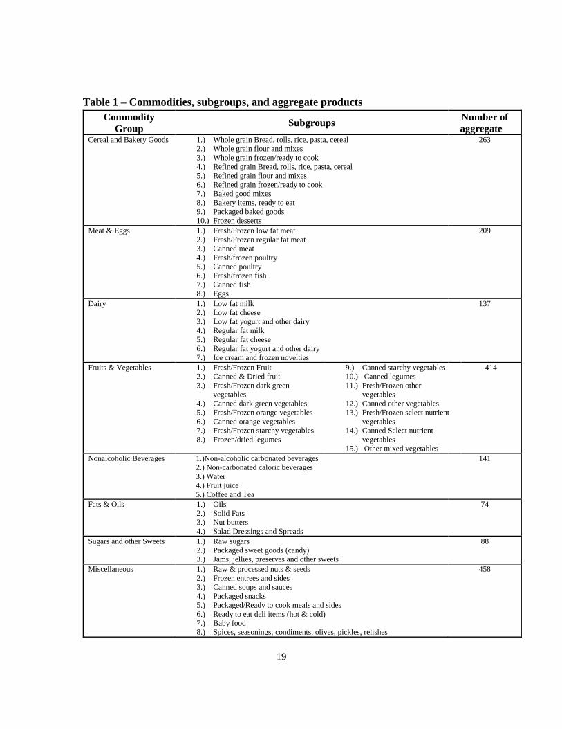
Price Database (QFAHPD) we consider eight commodity groups: 1) Cereal and Bakery

products, 2) Meats and Eggs, 3) Dairy, 4) Fruits and Vegetables, 5) Nonalcoholic

Beverages, 6) Fats and Oils, 7) Sugar and Other Sweets, and 8) Miscellaneous foods. Each

commodity group is itself composed of subgroups, identified in table 1.

To make data comparable across product sizes (e.g., ounces, pounds, etc.) all

product sizes were converted to grams following the method used by the QFAHPD and

price per 100g of product reported (Todd et al., 2010). Products with similar descriptions

and characteristics were aggregated using unit values into “aggregate products” following

the nutritional guideline-based methods of the QFAHPD. We further distinguished

“aggregate products” by brand type as a control for quality.3 The aggregate products were

identified as belonging to subgroups and then to one of the eight commodity groups. A list

7

of the commodity groups and subgroups is provided in table 1 along with the number of

aggregate products identified within that group. Using yogurt as an example: Dannon fat

free blueberry individual size yogurt and Dannon reduced fat strawberry quart-size yogurt

are treated as the same aggregate product: “Dannon-branded reduced fat yogurt,” within

the subgroup “Low fat yogurt and other dairy”, within the “Dairy” group.

Prices

To approximate a representative composite commodity price, researchers have adopted a

number of indexing methods. The index number represents the deviation of the price paid

by a household relative to the average household. Construction of a single price index to

represent a composite commodity is a multi-stage process involving: 1) Determination of

the price per unit for the aggregate food products, and 2) Construction of price indices for

the commodity groups.

The first stage involves the determination of a single price for a relatively

homogeneous-in-quality product. Following Diewert (1997) we use the unit value as the

elementary price at the aggregate food product level. The unit value for aggregate product

g in food commodity group j for household i (UV igj) is calculated as:

𝑈𝑉𝑔𝑗𝑖 =

∑ 𝑝𝑚𝑔𝑗𝑖 𝑞𝑚𝑔𝑗

𝑖𝑀𝑚=1

∑ 𝑞𝑚𝑔𝑗𝑖𝑀

𝑚=1 (1)

Where pimgj is household i’s price of the m brand in aggregate product g within the

commodity group j, and qimgj is household i’s quantity purchased of the m brand in

aggregate product g within the commodity group j. For some of the brand product

categories where prices pimgj are missing, prices were predicted following the methods

proposed by Meghir and Robin (1992) and Zhen et al. (2011) (see Leffler, 2012 for more

8

details). This required one regression over all households for each of the aggregate

commodities (1,784 regressions).

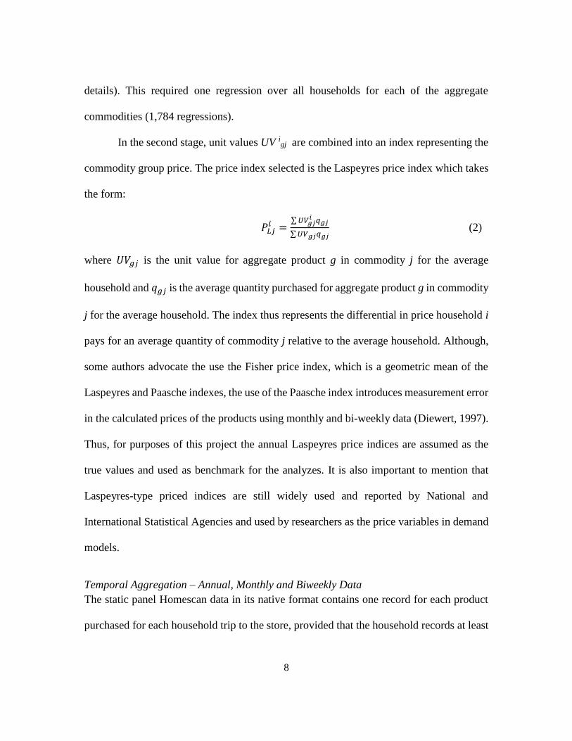
In the second stage, unit values UV igj are combined into an index representing the

commodity group price. The price index selected is the Laspeyres price index which takes

the form:

𝑃𝐿𝑗𝑖 =

∑ 𝑈𝑉𝑔𝑗𝑖 𝑞𝑔𝑗

∑ 𝑈𝑉𝑔𝑗𝑞𝑔𝑗 (2)

where 𝑈𝑉𝑔𝑗 is the unit value for aggregate product g in commodity j for the average

household and 𝑞𝑔𝑗 is the average quantity purchased for aggregate product g in commodity

j for the average household. The index thus represents the differential in price household i

pays for an average quantity of commodity j relative to the average household. Although,

some authors advocate the use the Fisher price index, which is a geometric mean of the

Laspeyres and Paasche indexes, the use of the Paasche index introduces measurement error

in the calculated prices of the products using monthly and bi-weekly data (Diewert, 1997).

Thus, for purposes of this project the annual Laspeyres price indices are assumed as the

true values and used as benchmark for the analyzes. It is also important to mention that

Laspeyres-type priced indices are still widely used and reported by National and

International Statistical Agencies and used by researchers as the price variables in demand

models.

Temporal Aggregation – Annual, Monthly and Biweekly Data

The static panel Homescan data in its native format contains one record for each product

purchased for each household trip to the store, provided that the household records at least

9

one trip per week for ten consecutive months. To provide a more manageable data set, we

aggregate household purchases to biweekly and monthly level. We only consider those

households in the “Fresh Foods Panel” and focused only on households in urban and

suburban locations with purchases in at least one commodity group.

We also aggregated household purchases to an annual level. Aggregating to an

annual level leaves a data set with 35,421 year-specific average monthly household

observations. The annual data is taken as a true measure of the demand for the food

commodities, owing to the longer period of observation. One month and 2-weeks data from

each household-specific year are randomly selected to comprise the monthly and biweekly

data set, respectively. This resulted in three data sets: 1) one with a record of a household’s

consumption for a year, 2) one with a record of a randomly selected month of consumption

for the same household in the same year, and 3) one with a record of a randomly selected

2-weeks of consumption for the same household in the same year. To make data

comparable between households with the biweekly and monthly data, the annual data was

transformed to average monthly data.4

Model Specification and Estimation

Preferences are assumed to be weakly separable, allowing models of household food at

home to be constructed independently of households’ other consumption choices (Meghir

and Robin 1992; Alfonso and Peterson 2006). Expenditures on the eight food commodity

groups identified previously are conditional on the broad food-at-home allocation (Gorman

1959). The demand systems are estimated using the Exact Affine Stone Index (EASI)

10

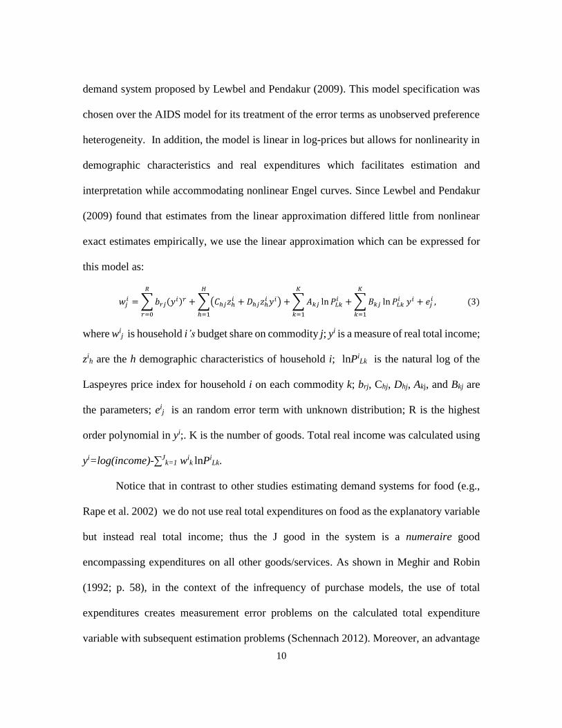
demand system proposed by Lewbel and Pendakur (2009). This model specification was

chosen over the AIDS model for its treatment of the error terms as unobserved preference

heterogeneity. In addition, the model is linear in log-prices but allows for nonlinearity in

demographic characteristics and real expenditures which facilitates estimation and

interpretation while accommodating nonlinear Engel curves. Since Lewbel and Pendakur

(2009) found that estimates from the linear approximation differed little from nonlinear

exact estimates empirically, we use the linear approximation which can be expressed for

this model as:

𝑤𝑗𝑖 = ∑ 𝑏𝑟𝑗(𝑦𝑖)𝑟 + ∑(𝐶ℎ𝑗𝑧ℎ

𝑖 + 𝐷ℎ𝑗𝑧ℎ𝑖 𝑦𝑖)

𝐻

ℎ=1

𝑅

𝑟=0

+ ∑ 𝐴𝑘𝑗 ln 𝑃𝐿𝑘𝑖 + ∑ 𝐵𝑘𝑗 ln 𝑃𝐿𝑘

𝑖 𝑦𝑖 + 𝑒𝑗𝑖

𝐾

𝑘=1

𝐾

𝑘=1

, (3)

where wij is household i’s budget share on commodity j; yi is a measure of real total income;

zih are the h demographic characteristics of household i; lnPi

Lk is the natural log of the

Laspeyres price index for household i on each commodity k; brj, Chj, Dhj, Akj, and Bkj are

the parameters; eij is an random error term with unknown distribution; R is the highest

order polynomial in yi;. K is the number of goods. Total real income was calculated using

yi=log(income)-∑Jk=1 w

ik lnPi

Lk.

Notice that in contrast to other studies estimating demand systems for food (e.g.,

Rape et al. 2002) we do not use real total expenditures on food as the explanatory variable

but instead real total income; thus the J good in the system is a numeraire good

encompassing expenditures on all other goods/services. As shown in Meghir and Robin

(1992; p. 58), in the context of the infrequency of purchase models, the use of total

expenditures creates measurement error problems on the calculated total expenditure

variable with subsequent estimation problems (Schennach 2012). Moreover, an advantage

11

of this approach relative to a conditional modeling approach is the estimation of

unconditional income and price elasticities which are more useful for policy analysis.

Estimation of the Annual Model

Since the annual data contains few zero observations on the dependent variables, the linear

approximation of the EASI demand system in equation (3) is estimated using Seemingly

Unrelated Regression (SUR). We impose the symmetry (Akj=Ajk, Bkj=Bjk ∀k,j) and

homogeneity (∑Kk=1 Akj = ∑

Kk=1 Bkj = 0 ∀j) restrictions. Following convention, the last

equation is dropped from the system and its parameters are recovered from the adding up

constraint. (Barten 1969 as cited in Barnett and Serletis 2008 p. 219; Lewbel and Pendakur

2009; and Zhen et al. 2011)

Estimation of Monthly and Bi-weekly Models

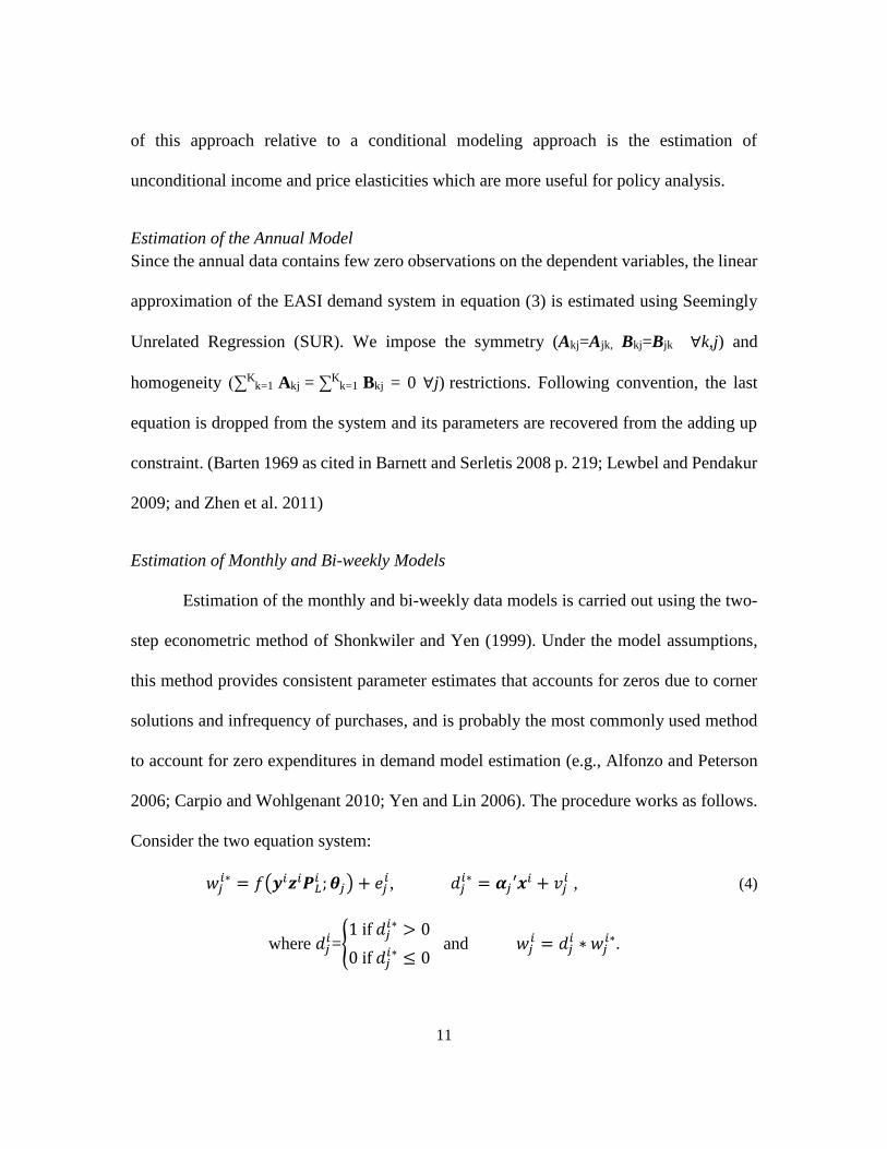
Estimation of the monthly and bi-weekly data models is carried out using the two-

step econometric method of Shonkwiler and Yen (1999). Under the model assumptions,

this method provides consistent parameter estimates that accounts for zeros due to corner

solutions and infrequency of purchases, and is probably the most commonly used method

to account for zero expenditures in demand model estimation (e.g., Alfonzo and Peterson

2006; Carpio and Wohlgenant 2010; Yen and Lin 2006). The procedure works as follows.

Consider the two equation system:

𝑤𝑗𝑖∗ = 𝑓(𝒚𝑖𝒛𝑖𝑷𝐿

𝑖 ; 𝜽𝑗) + 𝑒𝑗𝑖, 𝑑𝑗

𝑖∗ = 𝜶𝑗′𝒙𝑖 + 𝑣𝑗𝑖 , (4)

where 𝑑𝑗𝑖={

1 if 𝑑𝑗𝑖∗ > 0

0 if 𝑑𝑗𝑖∗ ≤ 0

and 𝑤𝑗𝑖 = 𝑑𝑗

𝑖 ∗ 𝑤𝑗𝑖∗.

12

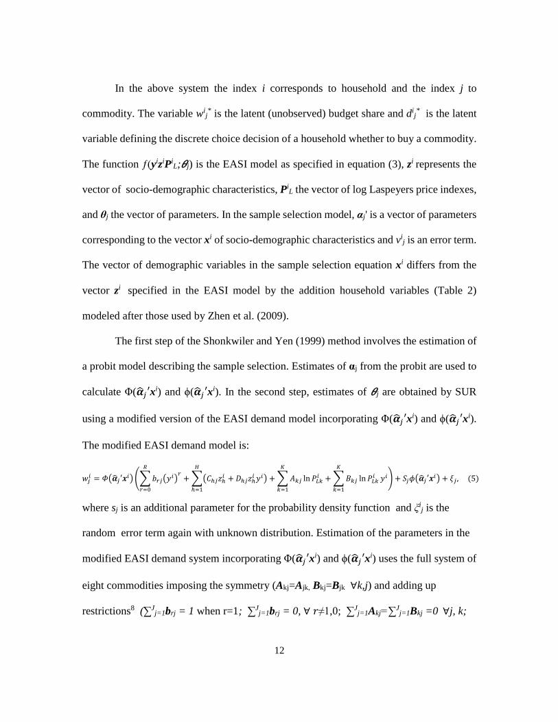
In the above system the index i corresponds to household and the index j to

commodity. The variable wij* is the latent (unobserved) budget share and di

j* is the latent

variable defining the discrete choice decision of a household whether to buy a commodity.

The function ƒ(yiziPiL;𝜃j) is the EASI model as specified in equation (3), zi represents the

vector of socio-demographic characteristics, PiL the vector of log Laspeyers price indexes,

and θj the vector of parameters. In the sample selection model, αj' is a vector of parameters

corresponding to the vector xi of socio-demographic characteristics and vij is an error term.

The vector of demographic variables in the sample selection equation xi differs from the

vector zi specified in the EASI model by the addition household variables (Table 2)

modeled after those used by Zhen et al. (2009).

The first step of the Shonkwiler and Yen (1999) method involves the estimation of

a probit model describing the sample selection. Estimates of αj from the probit are used to

calculate Φ(�̂�𝑗′xi) and ϕ(�̂�𝑗′xi). In the second step, estimates of 𝜃j are obtained by SUR

using a modified version of the EASI demand model incorporating Φ(�̂�𝑗′xi) and ϕ(�̂�𝑗′xi).

The modified EASI demand model is:

𝑤𝑗𝑖 = 𝛷(�̂�𝑗′𝒙𝑖) (∑ 𝑏𝑟𝑗(𝑦𝑖)

𝑟+ ∑(𝐶ℎ𝑗𝑧ℎ

𝑖 + 𝐷ℎ𝑗𝑧ℎ𝑖 𝑦𝑖)

𝐻

ℎ=1

𝑅

𝑟=0

+ ∑ 𝐴𝑘𝑗 ln 𝑃𝐿𝑘𝑖 + ∑ 𝐵𝑘𝑗 ln 𝑃𝐿𝑘

𝑖 𝑦𝑖

𝐾

𝑘=1

𝐾

𝑘=1

) + 𝑆𝑗𝜙(�̂�𝑗′𝒙𝑖) + 𝜉𝑗 , (5)

where sj is an additional parameter for the probability density function and ξij is the

random error term again with unknown distribution. Estimation of the parameters in the

modified EASI demand system incorporating Φ(�̂�𝑗′xi) and ϕ(�̂�𝑗′xi) uses the full system of

eight commodities imposing the symmetry (Akj=Ajk, Bkj=Bjk ∀k,j) and adding up

restrictions8 (∑Jj=1brj = 1 when r=1; ∑J

j=1brj = 0, ∀ 𝑟≠1,0; ∑Jj=1Akj=∑J

j=1Bkj =0 ∀j, k;

13

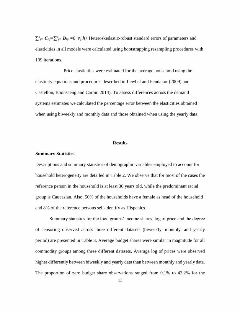
∑Jj=1Chj=∑J

j=1Dhj =0 ∀j,h). Heteroskedastic-robust standard errors of parameters and

elasticities in all models were calculated using bootstrapping resampling procedures with

199 iterations.

Price elasticities were estimated for the average household using the

elasticity equations and procedures described in Lewbel and Pendakur (2009) and

Castellon, Boonsaeng and Carpio 2014). To assess differences across the demand

systems estimates we calculated the percentage error between the elasticities obtained

when using biweekly and monthly data and those obtained when using the yearly data.

Results

Summary Statistics

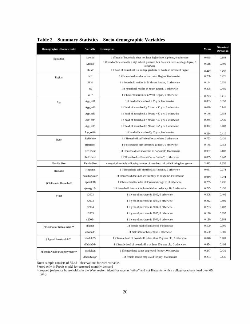
Descriptions and summary statistics of demographic variables employed to account for

household heterogeneity are detailed in Table 2. We observe that for most of the cases the

reference person in the household is at least 30 years old, while the predominant racial

group is Caucasian. Also, 50% of the households have a female as head of the household

and 8% of the reference persons self-identify as Hispanics.

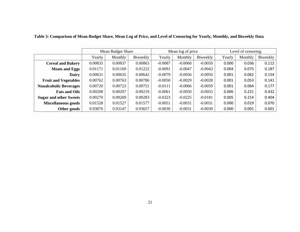
Summary statistics for the food groups’ income shares, log of price and the degree

of censoring observed across three different datasets (biweekly, monthly, and yearly

period) are presented in Table 3. Average budget shares were similar in magnitude for all

commodity groups among three different datasets. Average log of prices were observed

higher differently between biweekly and yearly data than between monthly and yearly data.

The proportion of zero budget share observations ranged from 0.1% to 43.2% for the

14

biweekly data and from 0.1% to 22.1% for the monthly data. The comparable percentages

for the yearly dataset ranged from 0% to 0.6%.

Comparison of Yearly Model vs. Monthly and Biweekly Models

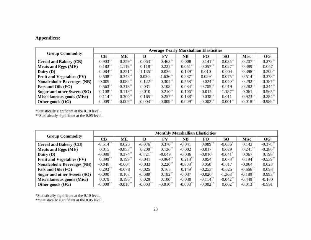
Estimation results for the demand systems for all datasets show the expected signs

for the income and own-price elasticities (see Appendices): all own price elasticities are

negative and all income elasticities are positive. To make our results comparable to those

of Gibson and Kim (2011) we first compare the estimated income elasticity values (Table

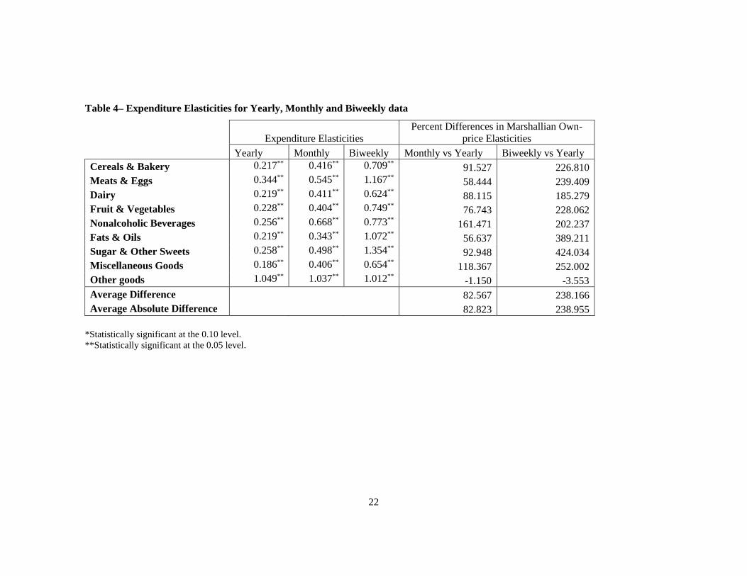
4). First, results in table 4 suggest that, except for the numeraire good, the demand model

using biweekly or monthly data provide substantially different food products income

elasticity estimates, compared to the demand model using yearly data. For example, in the

case of the biweekly elasticities, meats & eggs, fats & oils, and sugar & other sweets are

all luxuries according to the demand model using biweekly data, while the income

elasticities estimated by using yearly data are only all below 0.35. The differences between

biweekly and yearly food elasticities ranged from -3.5% to 425% difference, with an

average percent difference of 238%. Moreover, all the food products income elasticities

estimated using biweekly data were higher in order of magnitude.

Although the differences between monthly and yearly estimates are smaller, the

percentage error differences are still substantial ranging from a -1.1% difference to a 161%

percent difference, with an average difference of 82%. As in the case of the biweekly

elasticities, all the food products income elasticities estimated using monthly data were

higher in term of magnitude, except for the income elasticity of the numeraire good which

was slightly lower. It is also important to mention that the degree of linear correlation

15

between biweekly and yearly income elasticities and between monthly and yearly

elasticities were very different: 0.25 and 0.95, respectively.

It is important to mention the fact that the both the magnitude and the direction of

the income elasticity biases estimated in this study differ from the results of Gibson and

Kim (2007) study. First, they found that relative to the income elasticities estimated using

total consumption, elasticities estimated using an infrequency of purchase model and

shorter periods of time resulted in smaller income elasticity estimates. Our results find the

opposite, the use of shorter periods of time and a model to account for infrequency of

purchases tend to result in higher income elasticity estimates. However, the results are not

directly comparable since the baseline for comparison, the products analyzed, and the

econometric methods used for the estimation differ across studies. Regarding the baseline

for comparison, Gibson and Kim (2007) assumes that the “true” elasticities are those

estimated using total consumption which includes both change in stocks and acquisitions

during the period of observations (8 to 25 days). In contrast, our baseline for comparison

are the elasticities estimated using annual data. Regarding the products used for the

analysis, whereas Gibson and Kim (2007) tended to focused on specific goods, we used

aggregate food goods. Finally, whereas Gibson and Kim (2007) used univariate type of

analyses in the context of Engel equations with only income and socio-demographic

characteristics as explanatory variables in the equations, we used system demand

estimation approaches with income, prices and sociodemographic characteristics as

explanatory variables.

16

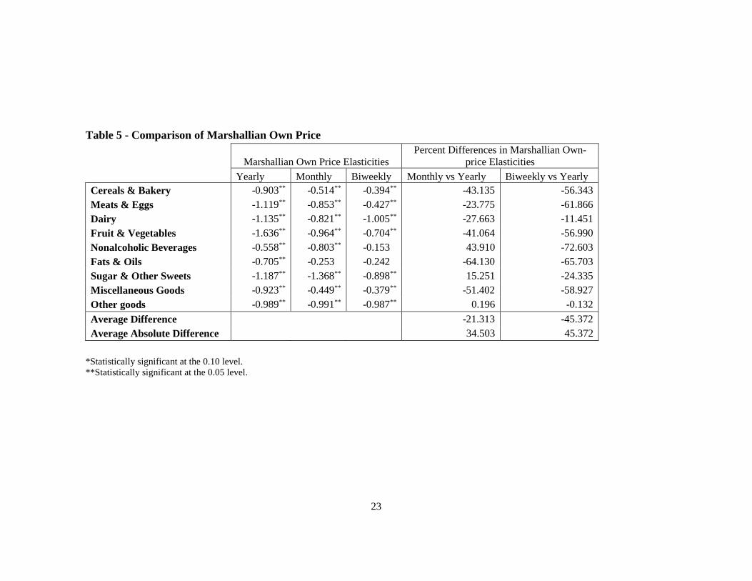
Regarding the comparison of own price elasticities obtained across the three

datasets, we found that, on average, the differences in terms of percentage errors were

smaller compared to the differences found with the income elasticities. The average

difference in terms of percentage errors between the yearly and biweekly own price

elasticities was 45%, whereas the difference between yearly and monthly own price

elasticities was 21%. Thus, in both cases, own price elasticities estimated using shorter

observation periods resulted, on average, in more inelastic own price elasticities (higher

values but lower absolute values). In addition, in the case of the biweekly model, all the

estimated own price elasticity values were more inelastic than the elasticities estimated

using the yearly model. In the case of the monthly model, although most (6 out of 9) of the

estimated own price elasticities were more inelastic, some (3 out of 8) were found to be

more elastic. Finally, we found similar linear correlation coefficients between yearly and

biweekly own price elasticities (0.61) and between yearly and monthly own price

elasticities (0.53).

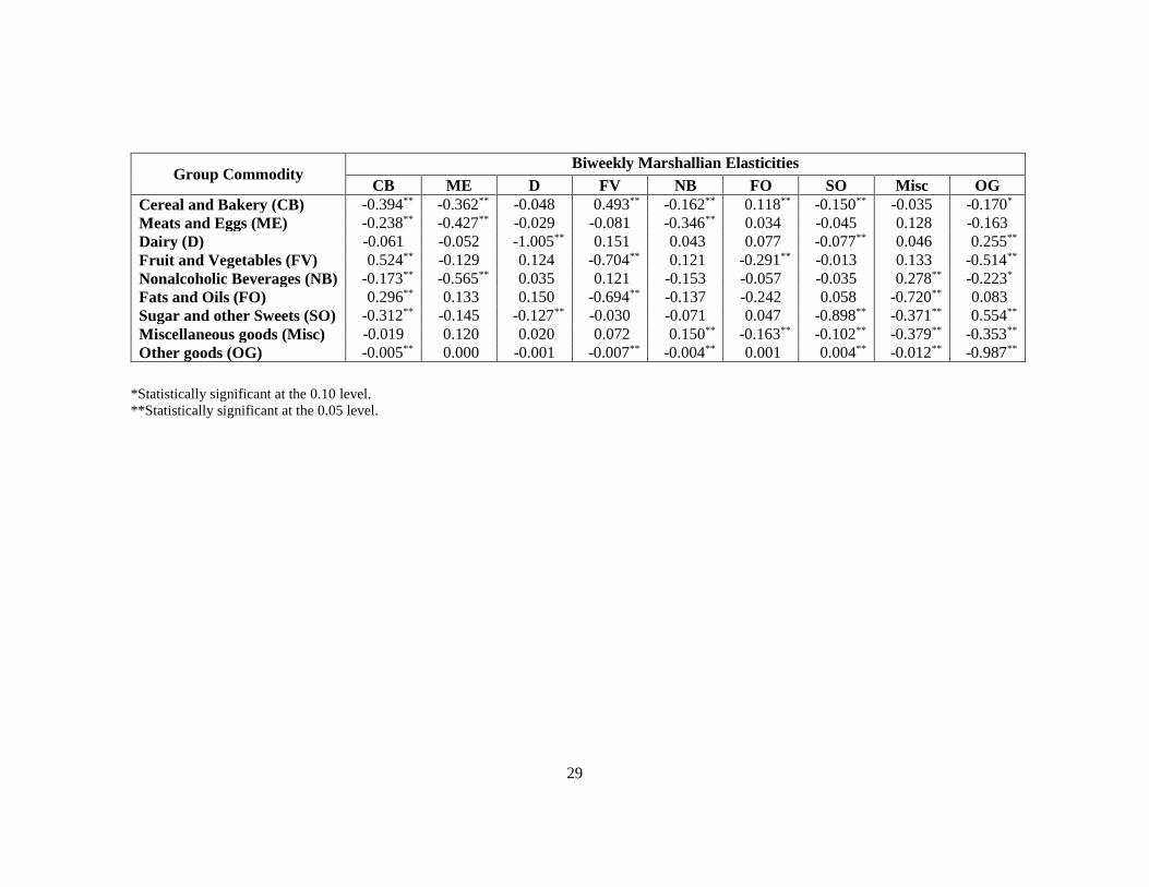
The differences between biweekly and yearly cross-price elasticities ranged from

-1089.83% to 1964.74%, with an average percent difference of 25.92%. The differences

between monthly and yearly cross-price elasticities are but still highly variable and range

from -477.13% to 870.31%, with an average difference of 9.35%. Mean absolute average

percent error for cross-price elasticities between biweekly and yearly data was 293.82%,

and 124.12% in the case of the difference between the monthly and yearly models.

With respect to the statistical significance of the elasticities (10% level), all the food

income elasticities using three different data periods were statistically significant. All eight

17

own-price elasticities from the model using yearly data were significant, and this number

decrease to seven and six own-price elasticities in the case of the monthly and biweekly

models, respectively. For cross price elasticities, 59 of 72 were statistically significant in

the yearly model, 40 in the monthly model and 31 in the biweekly model. Thus, in addition

to differences in the values of the elasticity estimates, the use of data at different levels of

temporal aggregations also seems to affect the ability of the models to detect statistical

significant differences from zero, especially in the case of price elasticities.

Summary and Conclusions

This article used an incomplete demand system for eight food commodity groups and five

years of data (2002-2006) from the Nielsen Homescan program. Three different levels of

temporal aggregation, biweekly, monthly and the average month within a year were

considered. Given the fact that the levels of censoring in the annual data are very small, we

conclude that the zero consumption values observed in the biweekly and monthly datasets

are due to the infrequency of purchase problem. Using elasticities obtained from the annual

dataset as the benchmark, we evaluate the performance of demand models estimated with

datasets from the shorter observation periods and an estimation procedures recommended

to account for the infrequency of purchases problem. Estimation results for the demand

systems for all datasets show the expected signs for the income and own-price elasticities.

All own price elasticities are negative and all income elasticities are positive. Biweekly

own price elasticities tended to be less elastic than annual elasticities and furthermore

biweekly income elasticities are more elastic than yearly elasticities.

18

Regarding the comparison of own price elasticities obtained across the three

datasets, we found that, on average, the differences in terms of percentage errors were

smaller compared to the differences found with the income elasticities. Furthermore, the

differences between monthly and yearly estimates for income, own-price, and cross-price

elasticities are smaller than the differences between biweekly and yearly for income, own-

price, and cross –price elasticities. We conclude that the monthly data more closely

approximates the underlying annual elasticities than the biweekly data.

In addition to differences in the values of the elasticity estimates, the use of data at

different levels of temporal aggregations also seems to affect the ability of the models to

detect statistical significant differences from zero, especially in the case of price

elasticities. We conclude that the data collection period does affect the value of elasticities

obtained from estimated food demand models. Moreover, larger biases in the estimated

elasticities are likely to be present even when using econometric methods currently

recommended to account for this problem.

19

Table 1 – Commodities, subgroups, and aggregate products

Commodity

Group Subgroups

Number of

aggregatets Cereal and Bakery Goods 1.) Whole grain Bread, rolls, rice, pasta, cereal

2.) Whole grain flour and mixes

3.) Whole grain frozen/ready to cook

4.) Refined grain Bread, rolls, rice, pasta, cereal

5.) Refined grain flour and mixes

6.) Refined grain frozen/ready to cook

7.) Baked good mixes

8.) Bakery items, ready to eat

9.) Packaged baked goods

10.) Frozen desserts

263

Meat & Eggs 1.) Fresh/Frozen low fat meat

2.) Fresh/Frozen regular fat meat

3.) Canned meat

4.) Fresh/frozen poultry

5.) Canned poultry

6.) Fresh/frozen fish

7.) Canned fish

8.) Eggs

209

Dairy 1.) Low fat milk

2.) Low fat cheese

3.) Low fat yogurt and other dairy

4.) Regular fat milk

5.) Regular fat cheese

6.) Regular fat yogurt and other dairy

7.) Ice cream and frozen novelties

137

Fruits & Vegetables 1.) Fresh/Frozen Fruit

2.) Canned & Dried fruit

3.) Fresh/Frozen dark green

vegetables

4.) Canned dark green vegetables

5.) Fresh/Frozen orange vegetables

6.) Canned orange vegetables

7.) Fresh/Frozen starchy vegetables

8.) Frozen/dried legumes

9.) Canned starchy vegetables

10.) Canned legumes

11.) Fresh/Frozen other

vegetables

12.) Canned other vegetables

13.) Fresh/Frozen select nutrient

vegetables

14.) Canned Select nutrient

vegetables

15.) Other mixed vegetables

414

Nonalcoholic Beverages 1.)Non-alcoholic carbonated beverages

2.) Non-carbonated caloric beverages

3.) Water

4.) Fruit juice

5.) Coffee and Tea

141

Fats & Oils 1.) Oils

2.) Solid Fats

3.) Nut butters

4.) Salad Dressings and Spreads

74

Sugars and other Sweets 1.) Raw sugars

2.) Packaged sweet goods (candy)

3.) Jams, jellies, preserves and other sweets

88

Miscellaneous 1.) Raw & processed nuts & seeds

2.) Frozen entrees and sides

3.) Canned soups and sauces

4.) Packaged snacks

5.) Packaged/Ready to cook meals and sides

6.) Ready to eat deli items (hot & cold)

7.) Baby food

8.) Spices, seasonings, condiments, olives, pickles, relishes

458

20

Table 2 – Summary Statistics – Socio-demographic Variables

Note: sample consists of 35,421 observations for each variable.

† used only in Probit model for censored monthly demand

ᵃ dropped (reference household is in the West region, identifies race as “other” and not Hispanic, with a college-graduate head over 65 yrs.)

Demographic Characteristic Variable Description MeanStandard

Deviation

Education LowEd 1 if head of household does not have high school diploma, 0 otherwise 0.035 0.184

MidEd1 if head of household is a high school graduate, but does not have a college degree, 0

otherwise0.518 0.500

HiEd ͣ 1 if head of household is a college graduate or holds an advanced degree 0.447 0.497

Region NE 1 if household resides in Northeast Region, 0 otherwise 0.238 0.426

MW 1 if household resides in Midwest Region, 0 otherwise 0.144 0.351

SO 1 if household resides in South Region, 0 otherwise 0.395 0.489

WT ͣ 1 if household resides in West Region, 0 otherwise 0.223 0.416

Age Age_ref1 1 if head of household < 25 yrs, 0 otherwise 0.003 0.050

Age_ref2 1 if head of household ≥ 25 and <30 yrs, 0 otherwise 0.020 0.141




Age_ref6 ͣ 1 if head of household ≥ 65 yrs, 0 otherwise 0.214 0.410

Race RefWhite 1 if Household self-identifies as white, 0 otherwise 0.753 0.431

RefBlack 1 if Household self-identifies as black, 0 otherwise 0.145 0.352

RefOrient 1 if Household self-identifies as “oriental”, 0 otherwise 0.037 0.188

RefOther ͣ 1 if Household self-identifies as “other”, 0 otherwise 0.065 0.247

Family Size FamilySize categorical variable indicating number of members 1-9 with 9 being 9 or greater. 2.412 1.356

Hispanic Hispanic 1 if Household self-identifies as Hispanic, 0 otherwise 0.081 0.274

nonHispanic ͣ 1 if Household does not self-identify as Hispanic, 0 otherwise 0.919 0.274

†Children in Household dperslt18 1 if household includes children under age 18, 0 otherwise 0.255 0.436

dpersgt18 ͣ 1 if household does not include children under age 18, 0 otherwise 0.745 0.436

†Year d2002 1 if year of purchase is 2002, 0 otherwise 0.208 0.406

d2003 1 if year of purchase is 2003, 0 otherwise 0.212 0.409



d2006 ͣ 1 if year of purchase is 2006, 0 otherwise 0.180 0.384

†Presence of female adult** dfadult 1 if female head of household, 0 otherwise 0.500 0.500

dmadult ͣ 1 if male head of household, 0 otherwise 0.500 0.500

†Age of female adult** dfadult35 1 if female head of household is less than 35 years old, 0 otherwise 0.046 0.209

dfadult36 ͣ 1 if female head of household is at least 35 years old, 0 otherwise 0.454 0.498

†Female Adult unemployment** dfadultun 1 if female head is not employed for pay, 0 otherwise 0.247 0.431

dfadultemp ͣ 1 if female head is employed for pay, 0 otherwise 0.253 0.435

21

Table 3: Comparison of Mean Budget Share, Mean Log of Price, and Level of Censoring for Yearly, Monthly, and Biweekly Data

Mean Budget Share Mean log of price Level of censoring

Yearly Monthly Biweekly Yearly Monthly Biweekly Yearly Monthly Biweekly

Cereal and Bakery 0.00835 0.00837 0.00863 -0.0087 -0.0060 -0.0050 0.000 0.036 0.112

Meats and Eggs 0.01171 0.01169 0.01222 -0.0091 -0.0047 -0.0043 0.004 0.075 0.187

Dairy 0.00631 0.00635 0.00642 -0.0079 -0.0056 -0.0050 0.001 0.062 0.154

Fruit and Vegetables 0.00762 0.00763 0.00786 -0.0050 -0.0029 -0.0028 0.001 0.053 0.141

Nonalcoholic Beverages 0.00720 0.00723 0.00751 -0.0111 -0.0066 -0.0059 0.001 0.064 0.177

Fats and Oils 0.00208 0.00207 0.00219 -0.0061 -0.0050 -0.0055 0.006 0.221 0.432

Sugar and other Sweets 0.00270 0.00269 0.00283 -0.0323 -0.0225 -0.0181 0.005 0.214 0.404

Miscellaneous goods 0.01528 0.01527 0.01577 -0.0051 -0.0031 -0.0031 0.000 0.019 0.070

Other goods 0.93876 0.93147 0.93657 -0.0030 -0.0031 -0.0030 0.000 0.001 0.001

22

Table 4– Expenditure Elasticities for Yearly, Monthly and Biweekly data

Expenditure Elasticities

Percent Differences in Marshallian Own-

price Elasticities

Yearly Monthly Biweekly Monthly vs Yearly Biweekly vs Yearly

Cereals & Bakery 0.217** 0.416** 0.709** 91.527 226.810

Meats & Eggs 0.344** 0.545** 1.167** 58.444 239.409

Dairy 0.219** 0.411** 0.624** 88.115 185.279

Fruit & Vegetables 0.228** 0.404** 0.749** 76.743 228.062

Nonalcoholic Beverages 0.256** 0.668** 0.773** 161.471 202.237

Fats & Oils 0.219** 0.343** 1.072** 56.637 389.211

Sugar & Other Sweets 0.258** 0.498** 1.354** 92.948 424.034

Miscellaneous Goods 0.186** 0.406** 0.654** 118.367 252.002

Other goods 1.049** 1.037** 1.012** -1.150 -3.553

Average Difference 82.567 238.166

Average Absolute Difference 82.823 238.955

*Statistically significant at the 0.10 level.

**Statistically significant at the 0.05 level.

23

Table 5 - Comparison of Marshallian Own Price

Marshallian Own Price Elasticities

Percent Differences in Marshallian Own-

price Elasticities

Yearly Monthly Biweekly Monthly vs Yearly Biweekly vs Yearly

Cereals & Bakery -0.903** -0.514** -0.394** -43.135 -56.343

Meats & Eggs -1.119** -0.853** -0.427** -23.775 -61.866

Dairy -1.135** -0.821** -1.005** -27.663 -11.451

Fruit & Vegetables -1.636** -0.964** -0.704** -41.064 -56.990

Nonalcoholic Beverages -0.558** -0.803** -0.153 43.910 -72.603

Fats & Oils -0.705** -0.253 -0.242 -64.130 -65.703

Sugar & Other Sweets -1.187** -1.368** -0.898** 15.251 -24.335

Miscellaneous Goods -0.923** -0.449** -0.379** -51.402 -58.927

Other goods -0.989** -0.991** -0.987** 0.196 -0.132

Average Difference -21.313 -45.372

Average Absolute Difference 34.503 45.372



24

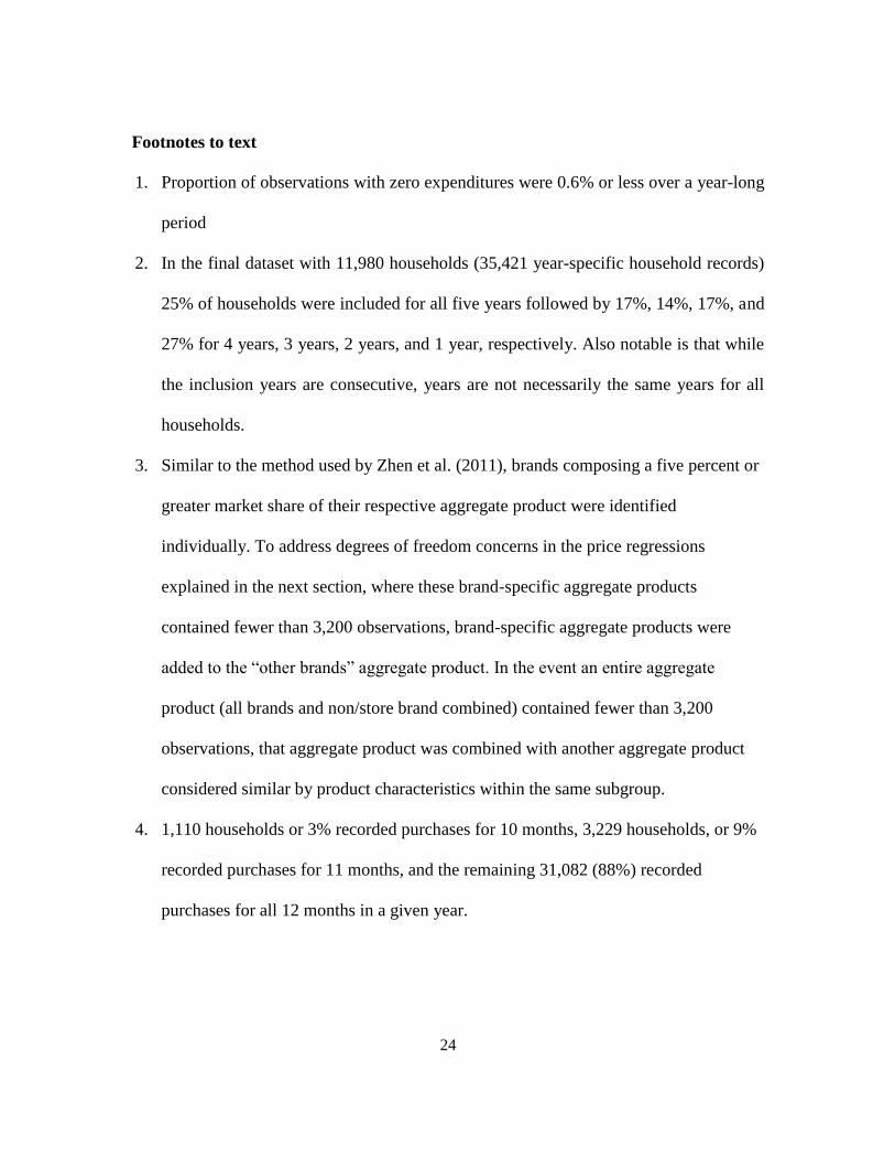
Footnotes to text

1. Proportion of observations with zero expenditures were 0.6% or less over a year-long

period

2. In the final dataset with 11,980 households (35,421 year-specific household records)

25% of households were included for all five years followed by 17%, 14%, 17%, and

27% for 4 years, 3 years, 2 years, and 1 year, respectively. Also notable is that while

the inclusion years are consecutive, years are not necessarily the same years for all

households.

3. Similar to the method used by Zhen et al. (2011), brands composing a five percent or

greater market share of their respective aggregate product were identified

individually. To address degrees of freedom concerns in the price regressions

explained in the next section, where these brand-specific aggregate products

contained fewer than 3,200 observations, brand-specific aggregate products were

added to the “other brands” aggregate product. In the event an entire aggregate

product (all brands and non/store brand combined) contained fewer than 3,200

observations, that aggregate product was combined with another aggregate product

considered similar by product characteristics within the same subgroup.

4. 1,110 households or 3% recorded purchases for 10 months, 3,229 households, or 9%

recorded purchases for 11 months, and the remaining 31,082 (88%) recorded

purchases for all 12 months in a given year.

25

References

Alfonzo, L., and H.H. Peterson. 2006. “Estimating Food Demand in Paraguay from

Household Survey Data.” Agricultural Economics, 34: 243-257.

Andreyeva, T, M.W. Long, and K.D. Brownell. 2010. “The Impact of Food Prices on

Consumption: A Systematic Review of Research on the Price Elasticity of

Demand for Food.” American Journal of Public Health, 100(2): 216-222.

Barnett, W.A., and A. Serletis. 2008. “Consumer Preferences and Demand Systems.”

Journal of Econometrics 147: 210-224.

Carpio, C.E., and M.K. Wohlgenant, 2010. “A General Two-Constraint Model of

Consumer Demand.” European Review of Agricultural Economics 37(4): 433–

452.

Castellon, C.E., Boonsaeng, T., and C.E., Carpio 2014. “Demand System Estimation in

the Absence of Price Data: An Application of Stone-Lewbel Price Indices.”

Applied Economics 47(6): 553-568.

Deaton, A. 1997. The Analysis of Household Surveys: A Microeconometric Approach to

Development Policy. Washington, DC: Johns Hopkins University Press.

Deaton, A., and M. Irish. 1984. “Statistical Models for Zero Expenditures in Budget

Shares.” Journal of Public Economics 23: 59-80.

Gibson, J., and B. Kim. 2012. “Testing the Infrequent Purchase Model Using Direct

Measurement of Hidden Consumption from Food Stocks.” American Journal of

Agricultural Economics 94(1):257-270.

Gorman, W.M. 1959. “Separable Utility and Aggregation.” Econometrica 21:63-80.

26

Keen, M. 1986. “Zero Expenditures and the Estimation of Engel Curves.” Journal of

Applied Econometrics 1(3):277-286.

Kinsey, J. and B. Senauer. 1996. “Consumer Trends and Changing Food Retailing

Formats.” American Journal of Agricultural Economics 78(5):1187-1191.

Leffler, K.K. 2012. “Temporal Aggregation and Treatment of Zero Dependent Variables in

the Estimation of Food Demand using Cross-Sectional Data.” Unpublished M.S.

thesis. The John E. Walker Department of Economics, Clemson University.

Lewbel, A., and K. Pendakur. 2009. “Tricks with Hicks: The EASI Demand System.”

American Economic Review 99:827-863.

Meghir, C., and J.M. Robin. 1992. “Frequency of Purchase and the Estimation of

Demand Systems.” Journal of Econometrics 53:53-85.

Okrent, A., and J.M. Alston. 2010. “The Demand for Food in the United States: A

Review of the Literature, Evaluation of Previous Estimates, and Presentation of

New Estimates of Demand.” Paper presented at AAEA annual meeting, Denver

CO, 25-27 July.

Park, J.L., R.B. Holcomb, K.C. Raper, and O. Capps. 1996. “A Demand Systems

Analysis of Food Commodities by U.S. Households Segmented by Income.”

American Journal of Agricultural Economics 78(2):290-300.

Raper, K.C., M.N. Wanazala, and R.M. Nayga. 2002. “Food Expenditures and Household

Demographic Composition in the US: A Demand Systems Approach.” Applied

Economics 34:981-992.

27

Schennach, S. M. (2012). Measurement error in nonlinear models: A review (No.

CWP41/12). cemmap working paper, Centre for Microdata Methods and Practice

Shonkwiler, J.S., and S.T. Yen. 1999. “Two-step Estimation of a Censored System of

Equations.” American Journal of Agricultural Economics 81:972-982.

Todd, J.E., L. Mancino, E. Leibtag, and C. Tripodo. 2010. Methodology behind the

Quarterly Food-At-Home Price Database. Washington DC: U.S. Department of

Agriculture, ERS for Technical Bulletin 1926, April.

Yen, S.T., and B.H. Lin. 2006. “A Sample Selection Approach to Censored Demand

Systems.” American Journal of Agricultural Economics 88:742-749.

Zhen, C., J.L. Taylor, M.K. Muth, and E. Leibtag. 2009. “Understanding Differences in

Self-Reported Expenditures Between Household Scanner Data and Diary Survey

Data: A Comparison of Homescan and Consumer Expenditure Survey.” Review of

Agricultural Economics 31(3):470-492.

Zhen, C., M.K. Wohlgenant, S. Karns, and P. Kaufman. 2011. “Habit Formation and

Demand for Sugar-sweetened Beverages.” American Journal of Agricultural

Economics 93(1):175-193.

28

Appendices:

Group Commodity Average Yearly Marshallian Elasticities

CB ME D FV NB FO SO Misc OG

Cereal and Bakery (CB) -0.903** 0.259** -0.063** 0.463** -0.008 0.141** -0.035** 0.207** -0.278**

Meats and Eggs (ME) 0.183** -1.119** 0.118** 0.222** -0.051** -0.057** 0.027** 0.389** -0.057

Dairy (D) -0.084** 0.221** -1.135** 0.036 0.139** 0.010 -0.004 0.398** 0.200**

Fruit and Vegetables (FV) 0.508** 0.343** 0.030 -1.636** 0.287** 0.029* 0.075** 0.514** -0.378**

Nonalcoholic Beverages (NB) -0.009 -0.082** 0.122** 0.304** -0.558** 0.024** 0.040** 0.292** -0.387**

Fats and Oils (FO) 0.563** -0.318** 0.031 0.108* 0.084** -0.705** -0.019 0.282** -0.244**

Sugar and other Sweets (SO) -0.108** 0.118** -0.010 0.210** 0.106** -0.015 -1.187** 0.061 0.565**

Miscellaneous goods (Misc) 0.114** 0.300** 0.165** 0.257** 0.138** 0.038** 0.011 -0.923** -0.284**

Other goods (OG) -0.009** -0.009** -0.004** -0.009** -0.009** -0.002** -0.001** -0.018** -0.989**



Group Commodity Monthly Marshallian Elasticities


Cereal and Bakery (CB) -0.514** 0.023 -0.076* 0.370** -0.041 0.089** -0.036* 0.142 -0.378**

Meats and Eggs (ME) 0.015 -0.853** 0.200** 0.126** -0.002 -0.017 0.029 0.241** -0.286**

Dairy (D) -0.098* 0.374** -0.821** -0.049 -0.036 -0.010 -0.041* 0.067 0.198*

Fruit and Vegetables (FV) 0.399** 0.199** -0.041 -0.964** 0.213** 0.054 0.078** 0.194* -0.539**

Nonalcoholic Beverages (NB) -0.048 -0.004 -0.033 0.220** -0.803** 0.050* -0.017 -0.064 0.028

Fats and Oils (FO) 0.293** -0.078 -0.025 0.165 0.149* -0.253 -0.025 -0.666** 0.093

Sugar and other Sweets (SO) -0.090* 0.107 -0.080* 0.182** -0.037 -0.020 -1.368** -0.189** 0.993**

Miscellaneous goods (Misc) 0.079 0.196** 0.029 0.100* -0.030 -0.114** -0.042** -0.449** -0.180

Other goods (OG) -0.009** -0.010** -0.003** -0.010** -0.003** -0.002** 0.002** -0.013** -0.991



29

Group Commodity Biweekly Marshallian Elasticities


Cereal and Bakery (CB) -0.394** -0.362** -0.048 0.493** -0.162** 0.118** -0.150** -0.035 -0.170*

Meats and Eggs (ME) -0.238** -0.427** -0.029 -0.081 -0.346** 0.034 -0.045 0.128 -0.163

Dairy (D) -0.061 -0.052 -1.005** 0.151 0.043 0.077 -0.077** 0.046 0.255**

Fruit and Vegetables (FV) 0.524** -0.129 0.124 -0.704** 0.121 -0.291** -0.013 0.133 -0.514**

Nonalcoholic Beverages (NB) -0.173** -0.565** 0.035 0.121 -0.153 -0.057 -0.035 0.278** -0.223*

Fats and Oils (FO) 0.296** 0.133 0.150 -0.694** -0.137 -0.242 0.058 -0.720** 0.083

Sugar and other Sweets (SO) -0.312** -0.145 -0.127** -0.030 -0.071 0.047 -0.898** -0.371** 0.554**

Miscellaneous goods (Misc) -0.019 0.120 0.020 0.072 0.150** -0.163** -0.102** -0.379** -0.353**

Other goods (OG) -0.005** 0.000 -0.001 -0.007** -0.004** 0.001 0.004** -0.012** -0.987**



data collection period and food demand system estimation...

Documents