Phase change, surface tension and turbulence inreal fluids

by

Daniel Albernaz

April 2016Technical Report

Royal Institute of TechnologyDepartment of Mechanics

SE-100 44 Stockholm, Sweden

Akademisk avhandling som med tillstand av Kungliga Tekniska Hogskolan iStockholm framlagges till offentlig granskning for avlaggande av teknologie dok-torsexamen fredagen den 7 April 2016 kl 10.15 i Kollegiesalen, Brinellvagen 8,Kungliga Tekniska Hogskolan, Stockholm.

©Daniel Albernaz 2016

Phase change, surface tension and turbulence in real fluids

Daniel L. AlbernazLinne FLOW Centre, KTH Mechanics, The Royal Institute of TechnologySE-100 44 Stockholm, Sweden

AbstractSprays are extensively used in industry, especially for fuels in internal combus-tion and gas turbine engines. An optimal fuel/air mixture prior to combustionis desired for these applications, leading to greater efficiency and minimal lev-els of emissions. The optimization depends on details regarding the differentbreakups, evaporation and mixing processes. Besides, one should take into con-sideration that these different steps depend on physical properties of the gasand fuel, such as density, viscosity, heat conductivity and surface tension.

In this thesis the phase change and surface tension of a droplet for differentflow conditions are studied by means of numerical simulations. This work ispart of a larger effort aiming to developing models for sprays in turbulent flows.We are especially interested in the atomization regime, where the liquid breakupcauses the formation of droplet sizes much smaller than the jet diameter. Thebehavior of these small droplets is important to shed more light on how toachieve the homogeneity of the gas-fuel mixture as well as that it directlycontributes to the development of large-eddy simulation (LES) models.

The numerical approach is a challenging process as one must take into ac-count the transport of heat, mass and momentum for a multiphase flow. Wechoose a lattice Boltzmann method (LBM) due to its convenient mesoscopicnature to simulate interfacial flows. A non-ideal equation of state is used tocontrol the phase change according to local thermodynamic properties. Weanalyze the droplet and surrounding vapor for a hydrocarbon fuel close to thecritical point. Under forced convection, the droplet evaporation rate is seen todepend on the vapor temperature and Reynolds number, where oscillatory flowscan be observed. Marangoni forces are also present and drive the droplet inter-nal circulation once the temperature difference at the droplet surface becomessignificant. In isotropic turbulence, the vapor phase shows increasing fluctu-ations of the thermodynamic variables once the fluid approaches the criticalpoint. The droplet dynamics is also investigated under turbulent conditions,where the presence of coherent structures with strong shear layers affects themass transfer between the liquid-vapor flow, showing also a correlation with thedroplet deformation. Here, the surface tension and droplet size play a majorrole and are analyzed in detail.

Descriptors: Evaporation, equation of state, hydrocarbon fuel, lattice Boltz-mann, deformation, droplet heating, critical point, Marangoni forces

iii

iv

Fasovergang, ytspanning och turbulens i icke-ideala fluider

Daniel L. AlbernazLinne FLOW Centre, KTH Mekanik, Kungliga Tekniska HogskolanSE-100 44 Stockholm, Sverige

SammanfattningSprayer anvands i stor utstrackning inom industri, sarskilt for branslen i for-brannings- och gasturbinmotorer. En optimal bransle/luft blandning fore for-branning ar onskvard for dessa tillampningar, vilket leder till stor effektivitetoch minimala nivaer av utslapp. Optimeringen beror pa detaljer angaende olikauppbrott, avdunstning och blandningsprocesser. Dessutom bor man beaktasatt dessa olika stegen ar beroende av fysikaliska egenskaper hos gas och bransle,sasom densitet, viskositet, varmeledningsformaga och ytspanning.

I den har avhandlingen kommer fasovergang och ytspanning hos en droppei olika flodestillstand att studeras genom numeriska simuleringar. Detta arbetear en del av ett storre projekt som siktar till att utveckla modeller for sprayeri turbulenta floden, vilket har betydelse for energiomvandling av branslen. Viar sarskilt intresserade av atomiseringsregimen, dar vatskan vid uppbrottetbildar droppstorlekar mycket mindre an straldiametern. Beteendet hos dessasma droppar ar viktigt for att tillfora ytterligare klarhet over hur man kanuppna homogenitet i gas-bransleblandningen, saval som den bidrar direkt tillutvecklingen av large-eddy simulation (LES) modeller.

Den numeriska metoden ar en utmanande process dar man maste beaktatransport av varme, massa och rorelsemangd for en flerfasstromning. Vi valjeren Lattice Boltzmann Method (LBM) pa grund av dess mesoskopiska naturatt simulera stromning med fria gransytor. En icke-ideal tillstandsekvationanvands for att styra fasomvandling baserat pa lokala termodynamiska egen-skaper. Vi undersoker droppen och kringliggande anga for ett kolvatebranslenara den kritiska punkten. Under patvingad konvektion synes en droppesforangningshastighet bero pa angtemperaturen och Reynolds tal, och os-cillerande floden kan observeras. Marangoni-krafter ar ocksa narvarande ochdriver pa droppens inre cirkulation nar temperaturskillnaden vid droppytan blirbetydande. I isotrop turbulens visar angfasen okande fluktuationer i de termo-dynamiska variablerna nar fluiden narmar sig den kritiska punkten. Dropp-dynamik undersoks ocksa i turbulens, dar forekomsten av sammanhangandestrukturer med starka skjuvskikt paverkar massoverforingen mellan vatske ochanga, som ocksa visar en korrelation med droppens deformation. Ytspanningoch droppstorlek har stort inflytande och analyseras i detalj.

Nyckelord: Avdunstning, tillstandsekvation, kolvatebransle, lattice Boltz-mann, deformation, droppe uppvarmning, kritisk punkt, Marangoni-krafter

v

vi

Preface

This thesis contains numerical investigations of phase change and surfacetension of a droplet for different flow conditions. Turbulent effects in singleand multiphase cases are also considered. The thesis is divided in two parts,where the first one presents an overview of the work and the main results. Thesecond part consists of five journal articles. The layout of these papers hasbeen adjusted to fit the format of this thesis, but their content has not beenchanged with respect to the original versions.

Paper 1.Albernaz, D. L., Do-Quang, M. & Amberg, G., 2013 Lattice BoltzmannMethod for the evaporation of a suspended droplet. Interfac. Phenom. HeatTransfer 1, 245-258

Paper 2.Albernaz, D. L., Do-Quang, M. & Amberg, G., 2015 Multirelaxation-time lattice Boltzmann model for droplet heating and evaporation under forcedconvection. Phys. Rev. E 91, 043012

Paper 3.Albernaz, D. L., Amberg, G. & Do-Quang, M., 2016 Simulation of asuspended droplet under evaporation with Marangoni effects. Accepted forpublication in Int. J. Heat Mass Transfer

Paper 4.Albernaz, D. L., Do-Quang, M., Hermanson, J. C. & Amberg, G.,2016 Real fluids near the critical point in isotropic turbulence. Under revisionfor publication in Phys. Fluids

Paper 5.Albernaz, D. L., Do-Quang, M., Hermanson, J. C. & Amberg, G.,2016 Droplet deformation and heat transfer in isotropic turbulence. Submittedto J. Fluid Mech.

vii

Division of work between authorsThe main advisor of the project is Prof. Gustav Amberg (GA) and the co-advisor is Dr. Minh Do-Quang (MDQ).

Paper 1The code was developed and implemented by Daniel Albernaz (DA). Simula-tions and analysis were carried out by DA. The paper was written by DA withfeedback from GA and MDQ.

Paper 2Implementations amd modifications were done by DA and MDQ, where thecode Palabos was used. DA performed the computations and analyzed thedata. The paper was written by DA with feedback from GA and MDQ.

Paper 3Implementations on the code, simulations and analysis were carried out by DA.The paper was written by DA with feedback from GA and MDQ.

Paper 4Modifications on the code were carried out by DA with help of MDQ. Thecomputations and analysis were performed by DA. The paper was written byDA with feedback from GA and MDQ. Prof. Jim Hermanson (JH) was alsoinvolved in discussions and provided feedback on the paper.

Paper 5Modifications on the code were carried out by DA. Simulations and analysiswere done by DA. The paper was written by DA with feedback from GA, MDQand JH.

viii

Part of the work has been presented at the following international conferences:

Albernaz, D. L., Do-Quang, M. & Amberg, G.Convective effects on evaporating droplet with the lattice Boltzmann method.11th International Conference for Mesoscopic Methods in Engineering and Sci-ence (ICMMES) – New York, USA, 2014

Albernaz, D. L., Do-Quang, M. & Amberg, G.Droplet dynamics in homogeneous isotropic turbulence. 68th Annual Meetingof the APS Division of Fluid Dynamics – Boston, USA, 2015

ix

x

If you’re not failing every now and again, it’s a sign you’renot doing anything very innovative.

Woody Allen, 1935–

xii

Contents

Abstract iii

Sammanfattning v

Preface vii

Part I - Overview & Summary

Chapter 1. Introduction 3

1.1. Fuel sprays: state of the art 4

1.2. Scope of the thesis 7

Chapter 2. Phase change 9

2.1. Equations of state 10

2.2. Clausius-Clapeyron relation 12

2.3. The D2 law 12

Chapter 3. Surface tension 15

3.1. The Young-Laplace law 15

3.2. Marangoni effect 16

Chapter 4. Turbulence 19

4.1. Homogeneous isotropic turbulence 21

Chapter 5. Numerical method 24

5.1. The lattice Boltzmann method 25

5.2. Energy equation 29

5.3. Validations and tests 31

Chapter 6. Summary of results 35

6.1. Forced convection 35

6.2. Turbulence with a single phase fluid 39

6.3. Droplet in isotropic turbulence 41

xiii

Chapter 7. Concluding remarks 46

Acknowledgements 49

Bibliography 50

Part II - Papers

Paper 1. Lattice Boltzmann Method for the evaporation of asuspended droplet 57

Paper 2. Multirelaxation-time lattice Boltzmann model fordroplet heating and evaporation underforced convection 77

Paper 3. Simulation of a suspended droplet under evaporationwith Marangoni effects 105

Paper 4. Real fluids near the critical point in isotropicturbulence 127

Paper 5. Droplet dynamics and heat transfer inisotropic turbulence 147

xiv

Part I

Overview & Summary

CHAPTER 1

Introduction

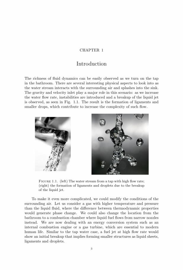
The richness of fluid dynamics can be easily observed as we turn on the tapin the bathroom. There are several interesting physical aspects to look into asthe water stream interacts with the surrounding air and splashes into the sink.The gravity and velocity inlet play a major role in this scenario: as we increasethe water flow rate, instabilities are introduced and a breakup of the liquid jetis observed, as seen in Fig. 1.1. The result is the formation of ligaments andsmaller drops, which contribute to increase the complexity of such flow.

Figure 1.1. (left) The water stream from a tap with high flow rate;(right) the formation of ligaments and droplets due to the breakupof the liquid jet.

To make it even more complicated, we could modify the conditions of thesurrounding air. Let us consider a gas with higher temperature and pressurethan the liquid fluid, where the difference between thermodynamic propertieswould generate phase change. We could also change the location from thebathroom to a combustion chamber where liquid fuel flows from narrow nozzlesinstead. We are now dealing with an energy conversion system such as aninternal combustion engine or a gas turbine, which are essential to modernhuman life. Similar to the tap water case, a fuel jet at high flow rate wouldshow an initial breakup that implies forming smaller structures as liquid sheets,ligaments and droplets.

3

4 1. INTRODUCTION

1.1. Fuel sprays: state of the art

The conventional understanding of spray formation when liquid leaves the noz-zle is based on the separation of the following stages (Lefebvre (1989)): develop-ment of a jet, conversion of a jet into liquid sheets and ligaments, disintegrationof ligaments into relatively large droplets (primary breakup) and breakup oflarge droplets into smaller ones (secondary breakup). The liquid jet may breakup into drops of widely different diameters, with sizes varying from the nozzlediameter down to droplets of diameters several orders of magnitude smaller.The size distribution is in general not uniform and depends on local flow con-ditions and properties of the fuel and gas.

Different dimensionless numbers can help describing the flow and breakupprocesses, among them the Reynolds number Re, which gives the ratio betweenthe inertial and viscous forces, and Weber number We that consists of theratio of inertia to surface tension force. Figure 1.2 shows a classical breakupregime given by a phase diagram between Re and We. The instability of aheavy fluid layer supported by a light one is known as Rayleigh instability andoccurs under an acceleration of the fluid system in the direction toward thedenser fluid (Rayleigh (1883)). This kind of instability is mainly observed inthe phase diagram when Re < 103 and We < 1. By increasing Re and/orWe by one order of magnitude, the jet becomes wavy due to aerodynamiceffects, known as the non-axisymmetric Rayleigh breakup. When Re is furtherincreased, the shear stresses at the gas/liquid interface strip off droplets. Fora given combination of Re and We a regime known as membrane breakup canbe obtained, where the whole round jet forms a thin sheet (membrane) beforebreaking into drops. When even larger Reynolds numbers are used, Re ∼ 105,short-wavelength shear instability takes place, known as atomization regime.Here, the disintegration process begins at the jet surface and gradually erodesthe jet until it is completely broken up, as seen in Fig. 1.31. Droplet sizesmuch smaller than the jet diameter can be observed. Atomization is achievedbeyond the upper bound of membrane breakup as seen in Fig. 1.2, and thefarther away from the bound, the finer the spray.

Experiments dealing with breakup of liquid jets are difficult due to the largenumber of droplets. When non-intrusive methods are used, the light is scatteredby the presence of these particles, making the spray opaque. Therefore, most ofthe available data is related to the average temporal development of the sprayby high-speed imaging or shadowgraphs (Dec (1997)). Regarding turbulentmixing, which can be measured by Laser Induced Fluorescence (LIF) as seenin Guillard et al. (1998), its combination with Particle Image Velocimetry (PIV)allows the simultaneous measurement of concentration and velocity field.

1Lasheras, J. C., Villermaux, E. & Hopfinger, E. J. 1998 Break-up and atomization of around water jet by a high-speed annular air jet. J. Fluid. Mech. 357, 351–379, Fig. 2 (g)

©Cambridge University Press.

1.1. FUEL SPRAYS: STATE OF THE ART 5

10-2

100

102

We

101

102

103

104

105

Re

Rayleigh

instability

wave-like

atomization

non-axisym.

Rayleigh

breakup

membrane

breakup

Figure 1.2. Breakup regimes of a jet given for a Re−We diagram.

Figure 1.3. Representation of a fuel liquid jet atomization for highRe number (left), where the formation of ligaments and dropletsmuch smaller than the jet diameter (right) are observed.

By combining these methods one is able to directly measure the turbulentfluxes of the fluid under consideration (Borg et al. (2001)). The recent intro-duction of high speed shutters (Sedarsky et al. (2007)) allows the capturing ofindividual droplets and filaments in the spray cloud. However, this method isstill under development and requires special equipment. Much still has to bedone in order to obtain experimental data for the wide range of scales thatcharacterize a spray with high Re number.

6 1. INTRODUCTION

When simulating atomization of liquid jets, the dominant method in in-dustrial applications consists of the Reynolds-averaged Navier-Stokes (RANS).In this method, drastic simplifications are made, where physical modelling ofatomization and sprays is an essential part of the two-phase flow computa-tion (Gorokhovski & Herrmann (2007)). Parameter tuning is usually necessarywith reference experimental data, and this should be done every time when theflow conditions are changed. In more advanced cases such as direct numericalsimulation (DNS) and large-eddy simulation (LES), physical modelling of at-omization and jets is still inevitable (Jiang et al. (2010)). For multiphase flows,there is no model-free DNS since the interactions between different phases needto be described. Even though detailed DNS with high resolution simulationshave been performed (e.g. Shinjo & Umemura (2010) and Shinjo & Umemura(2011)), there are also assumptions regarding surface tension forces and/ortemperature for droplets in the smallest scales.

Overall, fuel sprays are extensively applied in industry, where an opti-mal fuel/air mixture prior to combustion is desired, leading to best efficiencyand minimal levels of emissions (Shi et al. (2011)). In order to optimize fuelsprays, details regarding the different breakups, evaporation and mixing pro-cesses should be scrutinized and well understood. Besides, one should take intoaccount that these processes depend on physical properties of the gas and fuel,e.g. density, viscosity, heat conductivity and surface tension.

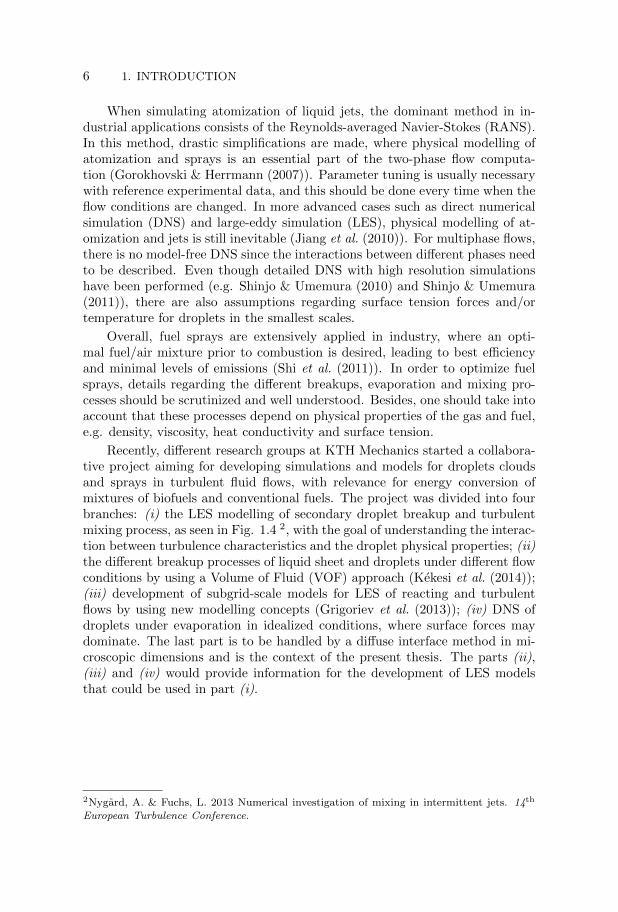
Recently, different research groups at KTH Mechanics started a collabora-tive project aiming for developing simulations and models for droplets cloudsand sprays in turbulent fluid flows, with relevance for energy conversion ofmixtures of biofuels and conventional fuels. The project was divided into fourbranches: (i) the LES modelling of secondary droplet breakup and turbulentmixing process, as seen in Fig. 1.4 2, with the goal of understanding the interac-tion between turbulence characteristics and the droplet physical properties; (ii)the different breakup processes of liquid sheet and droplets under different flowconditions by using a Volume of Fluid (VOF) approach (Kekesi et al. (2014));(iii) development of subgrid-scale models for LES of reacting and turbulentflows by using new modelling concepts (Grigoriev et al. (2013)); (iv) DNS ofdroplets under evaporation in idealized conditions, where surface forces maydominate. The last part is to be handled by a diffuse interface method in mi-croscopic dimensions and is the context of the present thesis. The parts (ii),(iii) and (iv) would provide information for the development of LES modelsthat could be used in part (i).

2Nygard, A. & Fuchs, L. 2013 Numerical investigation of mixing in intermittent jets. 14th

European Turbulence Conference.

1.2. SCOPE OF THE THESIS 7

Figure 1.4. Illustration of a LES simulation for an incompressibleliquid turbulent jet break-up.

1.2. Scope of the thesis

As we draw attention to the smaller scales in a fuel spray under an atomiza-tion regime, droplets between ≈ 0.2mm to nanoscales can be observed. Thesesmall droplets are more sensitive to local temperatures as they have largersurface area to volume ratio in comparison to larger ones. In other words,smaller droplets are heated up more quickly, which makes the evaporation pro-cess faster. The evaporation rate would depend on the flow condition andlocal thermodynamic properties. These droplets are also responsive to a turbu-lent environment: it is expected that the presence of coherent structures withstrong shear layers should affect the mass transfer between the liquid-vaporflows, where surface tension might also play an important role under certainconditions. The droplet behavior may shed more light on how to achieve thehomogeneity of the mixture of the fuel and the surrounding air.

The primary focus of this work is to numerically investigate the dynamics ofa single droplet in different flow conditions, where surface tension, phase changeand turbulent effects are analyzed in detail. This is an important step to gainin-depth insight into the different physical phenomena taking place inside a fueljet. Moreover, it contributes directly for modelling the smaller scales presentin fuel sprays, which consists in one of the goals from the collaborative projectbetween different research groups at KTH Mechanics. Although the studyof a single droplet dynamics may sound simple, the numerical approach is achallenging process as one must take into account the transport of heat, mass

8 1. INTRODUCTION

and momentum for a multiphase flow. We make use of a lattice Boltzmannmethod, shown as a promising method for dealing with interfacial flows as itcan address macro- and microscales. A non-ideal equation of state is used tocontrol the phase change according to local thermodynamic properties, where ahydrocarbon fuel is taken into consideration. In order to obtain a density ratioas observed in Diesel engines under operational conditions (between 20 and 65,as seen in Taylor (1985)), we analyze the droplet and surrounding vapor closeto the critical point.

The following chapters present the relevant theoretical and physical as-pects contained in this thesis. Chapter 2 describes the phase change, wherethe latent heat and different equations of state are discussed. The theoreticaldroplet heating and evaporation is also derived for a static condition. Chapter3 introduces the surface tension and the Marangoni effect. Chapter 4 gives abrief description of turbulence. Chapter 5 provides an overview of the numer-ical method used. We summarize the main results in Chapter 6 and presentconcluding remarks in Chapter 7.

CHAPTER 2

Phase change

A transition from one state of matter (solid or liquid or gas) to another withouta change in chemical composition is defined as phase change. During thistransition, a system either absorbs or releases a fixed amount of energy pervolume, changing the arrangement of the molecules as seen in Fig. 2.1. Thetemperature of the system stays constant as heat is added or taken from theprocess. The amount of heat q can be expressed as the product of the mass mand the specific latent heat L of the material, following

q = mL . (2.1)

The specific latent heat measures the change in enthalpy during the phasechange taken at constant temperature. In the case of phase transition fromliquid to vapor, the difference between the vapor and liquid enthalpies givesthe latent heat of vaporization Lhv, written as

Lhv = ∆h = hv − h` , (2.2)

where h is enthalpy and the subscripts v and ` denote the vapor and liquid,respectively. In evaporation, the energy added is used to break the bondsbetween the molecules. For a pure substance, liquid-vapor phase change alwaysoccurs at the saturation temperature. Since the phase change in our numericalmodel is controlled by an equation of state, some basic concepts are describedbelow.

Figure 2.1. Phase change between the states of matter, wheredifferent arrangement of molecules are obtained.

9

10 2. PHASE CHANGE

2.1. Equations of state

The expression equation of state (EOS) refers to equilibrium relationships in-volving pressure p, temperature T and specific volume υ (which can also bewritten in terms of density ρ, where υ = 1/ρ). If the vapor or gas can beapproximated as an ideal gas, the EOS is given as

pυ = RT , (2.3)

where R is the gas constant. It is known that an ideal EOS is inaccurate indescribing the behavior of many fluids, especially as critical point or saturationconditions are approached. In addition, an ideal gas EOS is of course incapableof modelling the liquid phase. A non-linear cubic EOS includes the interactionbetween molecules and takes into account a finite molecule volume. Theseconsiderations deviate from ideality and allow a non-ideal EOS to describeseveral fluids with good agreement, especially their liquid-vapor properties closeto the critical point. The van der Waals (vdW) EOS is the simplest and mostwell-known cubic EOS, given by

p =RT

υ − b− a

υ2, (2.4)

where a = 27(RTc)2/(64pc) is the attraction parameter and b = RTc/(8pc)

represents the volume occupied by the molecules of the substance, i.e. therepulsion parameter. The subscript c denotes the variable value at the criticalpoint. Different non-ideal EOS have been proposed in an effort to improve theEOS accuracy. Kaplun & Meshalkin (2003) proposed the M-K EOS which hasthe following form

p =RT

υ

(1 +

c′

υ − b′

)− a′

υ2, (2.5)

where a′, b′ and c′ are parameters used to fit the desired experimental data.Note that for b′ = c′, the vdW EOS is obtained. Another renowned EOS is thePeng-Robinson P-R EOS, given by

p =RT

υ − b− aα′(T )

υ2 + 2bυ − b2, (2.6)

with a = 0.45724R2T 2c /pc and b = 0.0778RTc/pc. The parameter α′(T ) =

[1 + (0.37464 + 1.54226w − 0.26992w2)(1 −√T/Tc)]

2 is defined according tothe acentric factor w and is a function of the actual temperature T . An EOSis useful for predicting the p − υ − T behavior of a fluid in a desired range ofvalues. A T −υ diagram can be used for finding the coexisting specific volumesof the liquid and vapor phases as a function of temperature. A curve in thisdiagram represents the saturated liquid and vapor lines.

In order to find the specific volumes analytically, a Maxwell constructioncould be used (Faghri & Zhang (2006)). The Maxwell construction, also known

2.1. EQUATIONS OF STATE 11

as the “equal area rule”, is derived from the condition that the free energies ofthe gas and the liquid must be equal when they coexist. The T − υ diagramof the fluid chosen for performing numerical simulations can be obtained byexperimental data. The comparison of the data to the Maxwell constructionfor a specific EOS is a way to evaluate if such EOS is suitable for represent-ing the desired fluid. Hydrocarbon fluids are common fuels when one has inmind the application of evaporating fuel in different engines. Throughout thisthesis we make use of a hexane fluid (C6H14), where the respective real val-ues are obtained from Lemmon et al. (2013). The acentric factor of hexane isw = 0.30075.

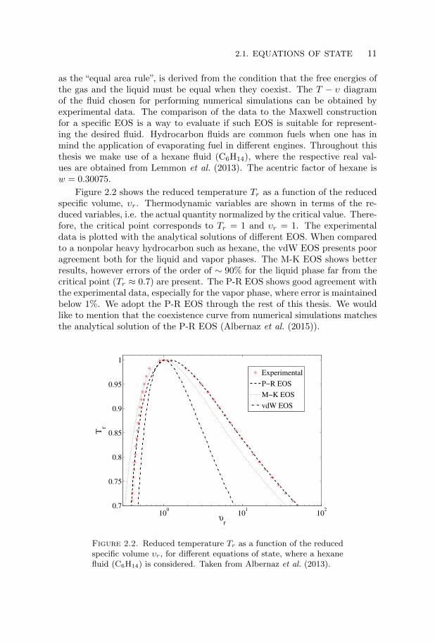
Figure 2.2 shows the reduced temperature Tr as a function of the reducedspecific volume, υr. Thermodynamic variables are shown in terms of the re-duced variables, i.e. the actual quantity normalized by the critical value. There-fore, the critical point corresponds to Tr = 1 and υr = 1. The experimentaldata is plotted with the analytical solutions of different EOS. When comparedto a nonpolar heavy hydrocarbon such as hexane, the vdW EOS presents pooragreement both for the liquid and vapor phases. The M-K EOS shows betterresults, however errors of the order of ∼ 90% for the liquid phase far from thecritical point (Tr ≈ 0.7) are present. The P-R EOS shows good agreement withthe experimental data, especially for the vapor phase, where error is maintainedbelow 1%. We adopt the P-R EOS through the rest of this thesis. We wouldlike to mention that the coexistence curve from numerical simulations matchesthe analytical solution of the P-R EOS (Albernaz et al. (2015)).

100

101

102

0.7

0.75

0.8

0.85

0.9

0.95

1

υr

Tr

Experimental

P−R EOS

M−K EOS

vdW EOS

Figure 2.2. Reduced temperature Tr as a function of the reducedspecific volume υr, for different equations of state, where a hexanefluid (C6H14) is considered. Taken from Albernaz et al. (2013).

12 2. PHASE CHANGE

2.2. Clausius-Clapeyron relation

An equilibrium state for two phases of a pure substance (single component) isgiven when both have the same temperature and pressure. If the temperatureof a two-phase system in equilibrium is changed slightly, the pressure of thesystem will be affected; this relationship is described by the Clausius-Clapeyronrelation (Faghri & Zhang (2006)). On a pressure-temperature P − T diagramone can also obtain the coexistence condition, which is characterized by a curvethat separates one phase from the other. The Clausius-Clapeyron relation givesthe slope of the tangents to this curve, and is written as

dP

dT=

∆s

∆υ, (2.7)

where dP/dT is the slope of the tangent to the coexistence curve at any point,∆s and ∆υ are the change in specific entropy and specific volume, respectively.The entropy change can be defined as the enthalpy variation divided by thethermodynamic temperature ∆s = ∆h/T . By using Eq. (2.2), entropy changeis rewritten as

∆s =LhvT

. (2.8)

The latent heat of vaporization can be explicitly expressed by combining thedefinition in Eq. (2.8) with Eq. (2.7), obtaining

Lhv = TdP

dT(υv − υ`) . (2.9)

Using the P-R EOS in Eq. (2.6) and for a certain temperature, the latent heatof vaporization in our model can be evaluated through the RHS of Eq. (2.9).The latent heat data obtained from Lemmon et al. (2013) matches with theone obtained in the model used.

2.3. The D2 law

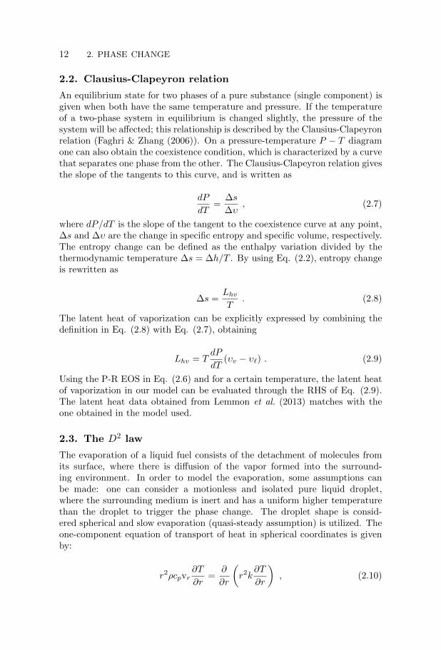
The evaporation of a liquid fuel consists of the detachment of molecules fromits surface, where there is diffusion of the vapor formed into the surround-ing environment. In order to model the evaporation, some assumptions canbe made: one can consider a motionless and isolated pure liquid droplet,where the surrounding medium is inert and has a uniform higher temperaturethan the droplet to trigger the phase change. The droplet shape is consid-ered spherical and slow evaporation (quasi-steady assumption) is utilized. Theone-component equation of transport of heat in spherical coordinates is givenby:

r2ρcpvr∂T

∂r=

∂

∂r

(r2k

∂T

∂r

), (2.10)

2.3. THE D2 LAW 13

where r is the radial distance from the droplet center, vr is the velocity in theradial direction and k is the thermal conductivity. The term cp represents thespecific volume at constant pressure, which is assumed constant as the slowevaporation has the implication of considering a limited temperature differencebetween the phases. It is important to note that in one-component evapora-tion the equation of transport of heat is sufficient due to the presence of onlyself-diffusion, i.e. the vapor is diffused into the surrounding vapor (Holyst et al.(2013)). The mass balance at the interface requires that the steady state va-por flux equals the evaporation rate at the droplet. Therefore, the continuityequation is given as

r2ρvr = r2i ρivi . (2.11)

By using Eq. (2.11) we integrate Eq. (2.10) with respect to r, which gives

r2i ρivicp

∂T

∂r= r2k

dT

dr+ constant , (2.12)

where the integration constant is determined from algebraic manipulations,according to the boundary condition given from the energy balance at theinterface, which assumes (Sirignano (2010))

R2kvdT

dr

∣∣∣i,v

= R2k`dT

dr

∣∣∣i,`

+R2ρiviLhv = R2ρiviLeff , (2.13)

where Leff denotes the effective latent heat of vaporization, R is the dropletradius and subscript i refers to quantities evaluated at the interface. The tem-perature of the entire droplet is generally considered constant, as the transportof heat inside the droplet is negligible, i.e. Leff = Lhv, which is also assumedin order to obtain an analytical solution. Using the boundary condition in Eq.(2.13), Eq. (2.12) becomes

r2i ρivicp

(T − Ti +

Lhvcp

)= r2k

dT

dr. (2.14)

After separating the variables we integrate Eq. (2.14) within the intervals[ri, r∞] and [Ti, T∞], obtaining

r2i ρivicpr

= ki ln

(T∞ − Ti + Lhv/cpT − Ti + Lhv/cp

), (2.15)

setting r equal to ri at the surface, we have

riviρicp = ki ln(1 +B) , (2.16)

where the nondimensional Spalding number B is given as

B =cp(T∞ − Ti)

Lhv. (2.17)

14 2. PHASE CHANGE

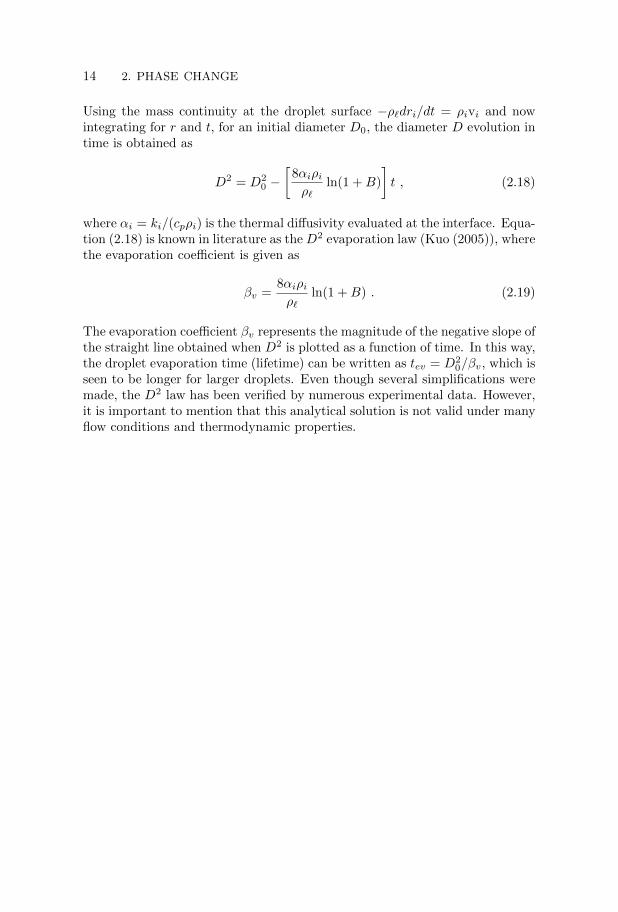
Using the mass continuity at the droplet surface −ρ`dri/dt = ρivi and nowintegrating for r and t, for an initial diameter D0, the diameter D evolution intime is obtained as

D2 = D20 −

[8αiρiρ`

ln(1 +B)

]t , (2.18)

where αi = ki/(cpρi) is the thermal diffusivity evaluated at the interface. Equa-tion (2.18) is known in literature as the D2 evaporation law (Kuo (2005)), wherethe evaporation coefficient is given as

βv =8αiρiρ`

ln(1 +B) . (2.19)

The evaporation coefficient βv represents the magnitude of the negative slope ofthe straight line obtained when D2 is plotted as a function of time. In this way,the droplet evaporation time (lifetime) can be written as tev = D2

0/βv, which isseen to be longer for larger droplets. Even though several simplifications weremade, the D2 law has been verified by numerous experimental data. However,it is important to mention that this analytical solution is not valid under manyflow conditions and thermodynamic properties.

CHAPTER 3

Surface tension

In a liquid there is an attractive force between molecules that is absent in gases.The surface tension is produced due to this difference between intermolecularforces at the liquid-vapor interface. Even though the interface is often treatedas a sharp discontinuity on the macroscale, the change of properties betweendifferent phases has a microscopic origin (Faghri & Zhang (2006)).

Near the interphase boundary, the density varies in space, and the interfa-cial energy can be computed as an excess energy of this inhomogeneous layer.If deformation occurs, both the shape and the area of the surface will affectthe internal energy of the interface. Therefore, surface tension is responsiblefor the shape of liquid droplets.

3.1. The Young-Laplace law

For a liquid droplet suspended in the vapor phase as illustrated in Fig. 3.1(left), the pressure inside is related to the vapor pressure by the Young-Laplaceequation

∆p = σ

(1

R1+

1

R2

), (3.1)

where R1 and R2 are the droplet radii of curvature in each of the axes thatare parallel to the surface and ∆p = p` − pv is the pressure difference betweenthe droplet interior and the vapor. The surface tension is denoted as σ. Fora spherical droplet, R1 = R2 = R. The Young-Laplace law can be obtainedfrom the force balance. In a half-sphere droplet, the surface tension force actsparallel to the surface, given as the surface tension times the circumference,σ2πR. In order to have a droplet in equilibrium, the opposite force due topressure difference times the area ∆pπR2 has to be of the same magnitude,where the equality becomes Eq. (3.1).

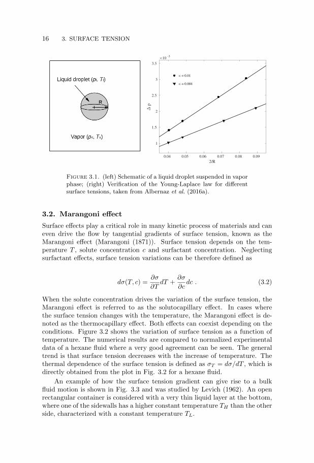
Figure 3.1 (right) shows the verification of the Young-Laplace law donefor our numerical model (in lattice units). Different values for the surfacetension can be achieved in the model by changing the interface thickness, whichis controlled by a dimensionless parameter κ (Markus & Hazi (2011)). Thesymbols indicate the numerical results whereas solid lines correspond to thetheoretical values, i.e. linear fit. It is observed that the linear dependence of∆p with 2/R is retrieved.

15

16 3. SURFACE TENSION

2/R

0.04 0.05 0.06 0.07 0.08 0.09

∆ p

×10-3

1

1.5

2

2.5

3

3.5

κ = 0.01

κ = 0.004

Figure 3.1. (left) Schematic of a liquid droplet suspended in vaporphase; (right) Verification of the Young-Laplace law for differentsurface tensions, taken from Albernaz et al. (2016a).

3.2. Marangoni effect

Surface effects play a critical role in many kinetic process of materials and caneven drive the flow by tangential gradients of surface tension, known as theMarangoni effect (Marangoni (1871)). Surface tension depends on the tem-perature T , solute concentration c and surfactant concentration. Neglectingsurfactant effects, surface tension variations can be therefore defined as

dσ(T, c) =∂σ

∂TdT +

∂σ

∂cdc . (3.2)

When the solute concentration drives the variation of the surface tension, theMarangoni effect is referred to as the solutocapillary effect. In cases wherethe surface tension changes with the temperature, the Marangoni effect is de-noted as the thermocapillary effect. Both effects can coexist depending on theconditions. Figure 3.2 shows the variation of surface tension as a function oftemperature. The numerical results are compared to normalized experimentaldata of a hexane fluid where a very good agreement can be seen. The generaltrend is that surface tension decreases with the increase of temperature. Thethermal dependence of the surface tension is defined as σT = dσ/dT , which isdirectly obtained from the plot in Fig. 3.2 for a hexane fluid.

An example of how the surface tension gradient can give rise to a bulkfluid motion is shown in Fig. 3.3 and was studied by Levich (1962). An openrectangular container is considered with a very thin liquid layer at the bottom,where one of the sidewalls has a higher constant temperature TH than the otherside, characterized with a constant temperature TL.

3.2. MARANGONI EFFECT 17

T

0.78 0.8 0.82 0.84 0.86 0.88 0.9

σ

0.02

0.03

0.04

0.05

0.06

LB simulations

Experimental

Figure 3.2. The surface tension is plotted as a function of thereduced temperature. Comparison between numerical results andexperimental data for a hexane fluid taken from Albernaz et al.

(2016a).

Figure 3.3. Thermocapillary motion in a shallow water.

The difference in side wall temperatures results in a temperature gradientalong the surface and a corresponding surface temperature gradient in the xdirection. The variation of surface tension is maintained and a thermocapillarymotion is generated at the interface, where the fluid height h is a function ofthe distance, i.e. h(x). To illustrate this, we assume a low Re number andneglect inertial terms, as well as lateral velocity gradients. For a steady two-dimensional incompressible flow, with constant liquid viscosity, the momentumequation in the x direction reduces to the Couette form

∂p

∂x= µ

∂2u

∂z2, (3.3)

and the z momentum equation without surface curvature effects is given as

∂p

∂z= −ρg . (3.4)

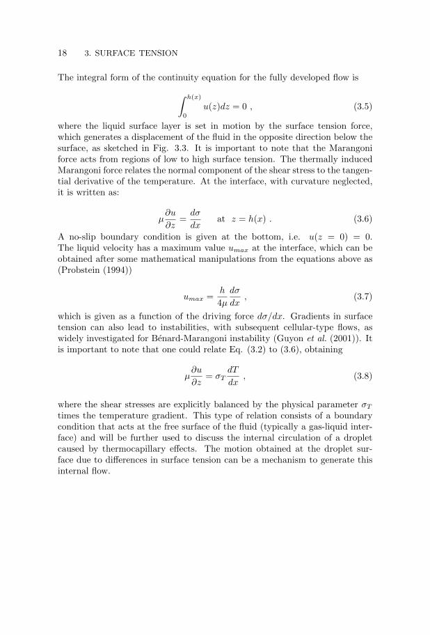
18 3. SURFACE TENSION

The integral form of the continuity equation for the fully developed flow is∫ h(x)

0

u(z)dz = 0 , (3.5)

where the liquid surface layer is set in motion by the surface tension force,which generates a displacement of the fluid in the opposite direction below thesurface, as sketched in Fig. 3.3. It is important to note that the Marangoniforce acts from regions of low to high surface tension. The thermally inducedMarangoni force relates the normal component of the shear stress to the tangen-tial derivative of the temperature. At the interface, with curvature neglected,it is written as:

µ∂u

∂z=dσ

dxat z = h(x) . (3.6)

A no-slip boundary condition is given at the bottom, i.e. u(z = 0) = 0.The liquid velocity has a maximum value umax at the interface, which can beobtained after some mathematical manipulations from the equations above as(Probstein (1994))

umax =h

4µ

dσ

dx, (3.7)

which is given as a function of the driving force dσ/dx. Gradients in surfacetension can also lead to instabilities, with subsequent cellular-type flows, aswidely investigated for Benard-Marangoni instability (Guyon et al. (2001)). Itis important to note that one could relate Eq. (3.2) to (3.6), obtaining

µ∂u

∂z= σT

dT

dx, (3.8)

where the shear stresses are explicitly balanced by the physical parameter σTtimes the temperature gradient. This type of relation consists of a boundarycondition that acts at the free surface of the fluid (typically a gas-liquid inter-face) and will be further used to discuss the internal circulation of a dropletcaused by thermocapillary effects. The motion obtained at the droplet sur-face due to differences in surface tension can be a mechanism to generate thisinternal flow.

CHAPTER 4

Turbulence

Turbulence appears much more often than we realize. Its presence may bedesirable, e.g. for applications as the mixing of different reactants in combustiondevices, where mixing has to occur as rapidly as possible, or undesirable, e.g.when drag is increased. An essential feature of turbulent flows is that the fluidvelocity field varies significantly and irregularly in both position and time. Inthis type of flow, unsteady vortices appear on many scales and interact witheach other, where the transport and mixing are much more effective than inthe laminar regime. For a laminar case, the fluid flows in parallel layers.

Richardson (1922) was the first to realize that turbulence is composed byeddies of different sizes. Large eddies are unstable and break down into smallerones that undergo a similar breakup process, so that energy is transferred to-ward smaller scales, until kinetic energy is converted into heat at the smallestscales of motion, where viscosity dominates. This is the concept of an energycascade, with energy transfer across several scales until molecular viscosity iseffective in dissipating the kinetic energy into internal energy. Kolmogorov(1941a) proposed hypotheses that led to the most important contribution toquantitative statistical description of turbulent flows. In the first hypothesis,he postulated that for high Reynolds numbers, the small-scale turbulent mo-tions are statistically isotropic. In general, large eddies are anisotropic andare affected by the boundary conditions of the flow (Pope 2000). Kolmogorovargued that the smaller eddies lose any preferred orientation, obtaining a localisotropy that is independent of the large-scale motions. The statistics of smallscales are universally dependent on the kinematic viscosity ν and the rate ofenergy dissipation ε. With only these two parameters, a length scale can beobtained by dimensional analysis as

η =

(ν3

ε

)1/4

, (4.1)

where η is known as the Kolmogorov length scale. The respective Kolmogorovvelocity and time scales are uη = (εν)1/4 and tη = (ν/ε)1/2. These scalescharacterize the smallest, dissipative eddies. The Reynolds number based onthese scales is unity, i.e. Reη = ηuη/ν = 1, indicating that viscous stresses andinertial forces balance at this level.

19

20 4. TURBULENCE

A turbulent flow can also be viewed as a superposition of a spectrum ofvelocity fluctuations and eddies upon a mean flow. A convenient way to dealmathematically with turbulent quantitites is to separate between the averageand fluctuating parts. This splitting is known as a Reynolds decomposition,which assumes e.g. for velocity ui

ui = ui + u′i , (4.2)

where ui denotes the time average and u′i the fluctuation part. In order toobtain the equation of motion for turbulent flows, we assume an incompressibleNavier-Stokes equation with a total instantaneous velocity given by

∂ui∂t

+ uj∂ui∂xj

= −1

ρ

∂p

∂xi+ ν

∂2ui∂xj∂xj

, (4.3)

where density ρ is considered constant. Introducing the Reynolds decomposi-tion for the velocity and pressure quantities, and taking the average gives

∂ui∂t

+ (uj + u′j)∂(ui + u′i)

∂xj= −1

ρ

∂p

∂xi+ ν

∂2ui∂xj∂xj

. (4.4)

The average of the fluctuating part and its derivatives are zero. For the incom-pressible condition ∂ui/∂xi = 0, Eq. (4.4) can be rewritten as

∂ui∂t

+ +uj∂ui∂xj

= −1

ρ

∂p

∂xi+

∂

∂xj

(ν∂ui∂xj− u′iu′j

). (4.5)

Equation (4.5) is known as the Reynolds-averaged Navier-Stokes (RANS) equa-tion, first proposed by Reynolds (1895). The change in mean momentum due tothe unsteadiness and convection of the mean flow is represented in the left handside of Eq. (4.5). The right hand side gives, respectively, the isotropic stressowing to the mean pressure field, the viscous stresses, and apparent stress owingto the fluctuating velocity field. This last term is referred to as the Reynoldsstress. It consists of a nonlinear tensor with symmetric properties, which hasled to the creation of many different turbulence models. By isolating the traceof this tensor one obtains the kinetic energy (per unit mass) of the turbulentfluctuations, defined as

E =1

2u′iu′i =

1

2

(u′21 + u′22 + u′23

). (4.6)

The turbulent kinetic energy can also be expressed in terms of the integral overwavenumber space, giving

E =

∫ ∞0

E(k)dk , (4.7)

where k denotes the wavenumber.

4.1. HOMOGENEOUS ISOTROPIC TURBULENCE 21

4.1. Homogeneous isotropic turbulence

Isotropic turbulence by direct numerical simulation has been extensively stud-ied (Ishihara et al. 2009). Homogeneity ensures that there are no gradientsin the mean turbulence statistics (invariance in translation) whereas isotropyleads to absence of anisotropy, i.e. no mean shear or buoyancy effects (invari-ance in rotation). Stationary turbulence is created by inserting energy intothe flow field through the low wavenumber modes so that a turbulent cascadedevelops as statistical equilibrium is reached.

In a DNS of homogeneous isotropic turbulence, the solution domain isa cube of side L with periodic boundary conditions. The lowest non-zerowavenumber in magnitude is k0 = 2π/L. The scalar wavenumber is givenas k = (k · k)1/2. For a high Reynolds number, the span of lengthscales willalso be large and it is possible to find a range of wavelengths that satisfy

η 2π

k L , or

1

L k 1

η. (4.8)

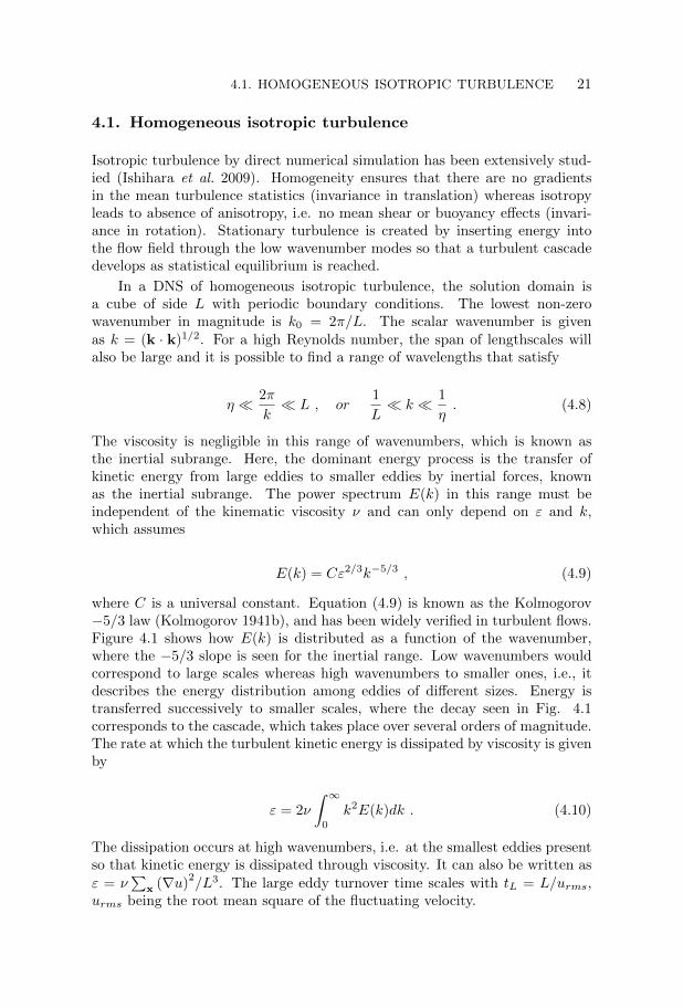
The viscosity is negligible in this range of wavenumbers, which is known asthe inertial subrange. Here, the dominant energy process is the transfer ofkinetic energy from large eddies to smaller eddies by inertial forces, knownas the inertial subrange. The power spectrum E(k) in this range must beindependent of the kinematic viscosity ν and can only depend on ε and k,which assumes

E(k) = Cε2/3k−5/3 , (4.9)

where C is a universal constant. Equation (4.9) is known as the Kolmogorov−5/3 law (Kolmogorov 1941b), and has been widely verified in turbulent flows.Figure 4.1 shows how E(k) is distributed as a function of the wavenumber,where the −5/3 slope is seen for the inertial range. Low wavenumbers wouldcorrespond to large scales whereas high wavenumbers to smaller ones, i.e., itdescribes the energy distribution among eddies of different sizes. Energy istransferred successively to smaller scales, where the decay seen in Fig. 4.1corresponds to the cascade, which takes place over several orders of magnitude.The rate at which the turbulent kinetic energy is dissipated by viscosity is givenby

ε = 2ν

∫ ∞0

k2E(k)dk . (4.10)

The dissipation occurs at high wavenumbers, i.e. at the smallest eddies presentso that kinetic energy is dissipated through viscosity. It can also be written asε = ν

∑x (∇u)

2/L3. The large eddy turnover time scales with tL = L/urms,

urms being the root mean square of the fluctuating velocity.

22 4. TURBULENCE

10-2

10-1

100

wavenumber

10-20

10-15

10-10

10-5

E(k

)

-5/3

Energy flow

Inertial rangeViscous

dissipation

Figure 4.1. Energy spectrum as a function of the wavenumber.

Another important length scale is the Taylor microscale, defined in termsof the square root of the ratio between variances of the velocity and velocitygradient, following

λ =

[15νu2

rms

ε

]1/2

. (4.11)

The Taylor microscale signifies an intermediate length scale at which fluid vis-cosity still affects the dynamics of turbulent eddies in the flow, however it isnot a dissipative scale. The Taylor microscale is traditionally applied to a tur-bulent flow, which can be characterized by a Kolmogorov spectrum of velocityfluctuations, as in isotropic turbulence. A Taylor Reynolds number is obtainedwhen considering this microscale, which becomes

Reλ =urmsλ

ν. (4.12)

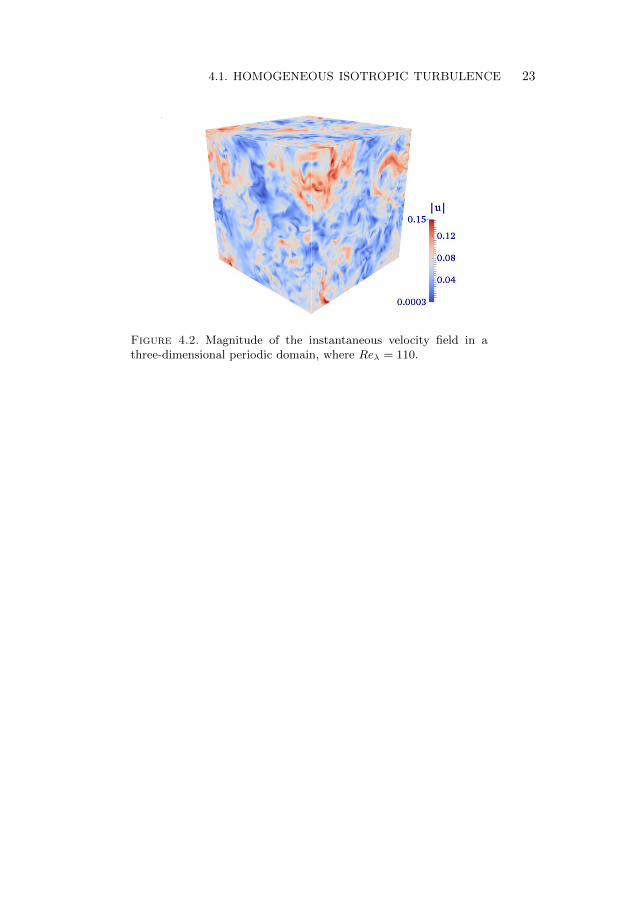
Developed isotropic turbulence is illustrated in Figure 4.2 by showing the in-stantaneous magnitude of the velocity field. The Taylor Reynolds number usedin this simulation is Reλ = 110.

4.1. HOMOGENEOUS ISOTROPIC TURBULENCE 23

Figure 4.2. Magnitude of the instantaneous velocity field in athree-dimensional periodic domain, where Reλ = 110.

CHAPTER 5

Numerical method

The numerical simulation of flows with phase change is challenging due tothe evolving nature of the fluid-fluid interface. It is essential to couple theinterfacial mass transfer, latent heat and surface tension in accordance withthe relevant conservation of mass, momentum and energy. There are variousnumerical schemes which can be used for the direct numerical simulation ofgas-liquid flows. For Navier-Stokes solvers, i.e. based on the discretizationof macroscopic governing equations, the volume of fluid method (Scardovelli &Zaleski (1999)), level set method (Sethian & Smereka (2003)) and front trackingmethod (Tryggvason et al. (2001)) are the most common methods used.

Different methods have been applied to investigate droplet evaporation.Tanguy et al. (2007) developed a level set method associated with the ghostfluid method to enable higher order discretization schemes at the interface.Zhang (2003) and Balaji et al. (2011) used a finite volume method where thedroplet maintains a spherical shape. A volume of fluid method (VOF) was usedby Hase & Weigand (2004) where strong deformations are captured. Schlottke& Weigand (2008) improved the same VOF code to perform direct numeri-cal simulations of droplet evaporation. VOF was also used by Strotos et al.(2011) and Banerjee (2013) where a multicomponent droplet was considered.Although each method has a different approach, in order to satisfy conserva-tion conditions, a local vaporizing mass flow rate has to be set explicitly, whichis usually done by means of a reference experimental data. An evaporationmodel often introduces different simplifications, e.g. non deformable droplet(axisymmetric evaporation) or the assumption of constant gas physical proper-ties (quasi-steady). The available evaporation models can be found in reviewsby Sazhin (2006) and Erbil (2012).

Unlike the conventional numerical methods previously mentioned, Molec-ular Dynamics (MD) and lattice Boltzmann method (LBM) are two methodswhere no tracking method is needed for generating an interface. The phasesegregation can emerge naturally as a result of particle interactions. MD isused for simulating the physical movements of atoms and molecules, wheremany degrees of freedom are present. A common method in this category isthe Monte Carlo molecular method, which is based on states according to ap-propriate Boltzmann probabilities. The drawback of MD is due to the largeamount of molecules needed for simulating macroscopic flows and the simulatedtime, which at present is in the order of nanoseconds.

24

5.1. THE LATTICE BOLTZMANN METHOD 25

The LBM is becoming an increasingly important method for simulatingmultiphase flows (Sukop & Thorne (2006)). It is in the category of diffuseinterface methods and is based on a mesoscopic kinetic equation for particledistribution functions (Chen & Doolen (1998)). The mesoscopic approach is asimplification of MD, where instead of simulating every molecule one takes intoconsideration a group of molecules which are confined at nodes and move in adiscrete number of directions, as illustrated in Fig. 5.1. By averaging the kineticequations one reproduces the Navier-Stokes equations at the macroscopic level.

Figure 5.1. Macro-, meso- and microscale for the numerical modelling.

The mesoscopic nature of LBM includes only a minimal amount of mi-croscopic details in order to reproduce interfacial physics and macroscopic flowhydrodynamics in a consistent manner (Safari et al. (2013)). Its nature is there-fore responsible for avoiding the need for tracking the interface as it bridgesmicroscopic phenomena and the macroscopic scale. It also presents a convenientframework to incorporate thermodynamic effects, which naturally generate thephase separation. The kinetic equation provides also the advantages of easyimplementation of boundary conditions and fully parallel algorithms. Becauseof the current availability of fast and massively parallel machines, there is atrend to use codes that can exploit the intrinsic features of parallelism, whichis the case of the LBM.

5.1. The lattice Boltzmann method

The lattice Boltzmann model is constructed as a simplified, fictitious moleculardynamics method in which space, time, and particle velocities are all discrete.In other words, the LBM vastly simplifies Boltzmann’s original conceptual viewby reducing both the number of possible particle spatial positions and thecontinuum microscopic momenta. Particle positions are confined to the nodesof the lattice, which is characterized as a regular grid. The lattice Boltzmannequation is given by

fi(x + ciδt, t+ δt)− f(x, t) = δtΩi + δtF′i , (5.1)

where fi is the density distribution function, t is time and δt is the time step.The lattice velocity is given by ci, x is the spatial position and F ′ is an external

26 5. NUMERICAL METHOD

forcing term, which can include e.g. gravity forces or interparticle interactions.The change of fi due to collisions is represented by Ωi. The notation i is givenas i = 0, . . . , N , where N denotes the number of directions of the particlevelocities at each node. For two-dimensional simulations a lattice with nine-velocity directions is recommended (D2Q9), while a nineteen-velocity lattice isusually applied for three-dimensional calculations (D3Q19).

Starting from an initial state, the configuration of particles at each timestep evolves in two sequential sub-steps, described as (i) streaming, which isgiven by the LHS of Eq. (5.1), where each particle moves to the nearest nodein the direction of its velocity; and (ii) collision, which occurs when particlesarriving at a node interact and change their velocity directions according toscattering rules. It is important to note that the streaming process of the LBMis linear. This feature comes directly from the kinetic theory and contrastswith the nonlinear convection terms in other numerical approaches that usea macroscopic representation. Simple convection combined with a collisionoperator allows the recovery of the nonlinear macroscopic advection throughmulti-scale expansions, which turns out to be one big advantage when dealingwith LBM. The macroscopic fluid quantities, such as density and velocity, arecalculated by

ρ =

N∑i=0

fi , u =1

ρ

N∑i=0

cifi . (5.2)

The macroscopic velocity u is an average of the discretized microscopic veloc-ities ci weighted by the directional densities fi. Different collision operatorshave been proposed. A simple linearized version of the collision operator makesuse of a relaxation time towards the local equilibrium using a single time re-laxation. This collision model is known as the Bhatnagar-Gross-Krook (BGK),which was proposed by Bhatnagar et al. (1954) and is written as

Ωi = −fi − feqi

τf, (5.3)

where feq is a local equilibrium distribution, which has to be formulated sothat the Navier-Stokes equations are recovered in the macroscopic scale. Inorder to do so, the equilibrium function has to be defined as

feqi = ωiρ

[1 +

ci · uc2s

+(ci · u)2

2c4s− u · u

2c2s

], (5.4)

where cs is the sound speed and ωi are the weights according to the latticechosen. By using the BGK collision operator, the kinematic viscosity ν isdenoted as

ν = c2s(τf − 1/2) . (5.5)

5.1. THE LATTICE BOLTZMANN METHOD 27

We would like to mention that although the BGK model is widely used dueto its simplicity, it is numerically unstable under certain conditions, e.g. forhigh Reynolds numbers where lower values of the fluid viscosity are necessary.This can be solved by using a more robust collision operator. The multiple-relaxation-time model (MRT) proposed by Lallemand & Luo (2000) allowsfor different physical quantities to be adjusted independently and has shownsignificant improvement in the numerical stability. If body forces acting on afluid are absent, i.e. F ′i = 0 in Eq. (5.1), the equation of state for this modelassumes the form as for an ideal gas, where

p = ρc2s . (5.6)

However, with the idea of simulating a vapor-liquid flow, F ′i should be used.In LBM, the phase segregation can be modelled by an interaction force, i.e. aspecial mesoscospic force which acts between every pair of neighboring nodes.Shan & Chen (1993) proposed the pseudopotential model, where this interac-tion force is calculated from an interaction potential ψ. For single-componentmultiphase flows, the force is given by

F = ψ(ρ(x))G

N∑i=1

ψ(ρ(x + ci))ci , (5.7)

where G is the interaction strength. We note that the potential is dependenton the local fluid density. For this force, the equation of state (EOS) has theform (He & Doolen (2002))

p = ρc2s −Gc2

2Ψ2 , (5.8)

where c is a lattice constant. Many discussions have been made on how tochoose the potential ψ. The only way to satisfy both the mechanical sta-bility solution (Maxwell construction) and the thermodynamic theory is ifψ ∝ exp(−1/ρ), as shown by Shan & Chen (1994). If one wants to include anarbitrary EOS, a different approach is recommended. We adopted a methodproposed by Kupershtokh et al. (2009), where the force is given as

F = 2Φ∇Φ, (5.9)

where Φ is a special function written as

Φ =√ρc2s − κp(ρ, T ) , (5.10)

here p(ρ, T ) can be based on an arbitrary EOS. The term κ denotes a dimen-sionless parameter that controls the interface thickness in lattice units. Ku-pershtokh et al. (2009) also proposed a numerical approximation for the local

28 5. NUMERICAL METHOD

force based on a linear combination of the local and the mean value gradientapproximations, calculated by

F =A

c2s

N∑i=1

λiΦ2(x + ci)ci +

(1− 2A)

c2sΦ(x)

N∑i=1

λiΦ(x + ci)ci , (5.11)

where A is a correlative fitting parameter that allows a better fit with thecoexistence curve for the desired fluid, satisfying the Maxwell construction.The value of A changes according to the EOS adopted. Equation (5.11) is anumerical approximation for the local force based on a linear combination of thelocal and the mean value gradient and improves the numerical stability, wherethe spurious currents around the interface are significantly reduced. Thesecurrents are a common problem in simulations with free boundaries. The useof Eq. (5.11) is followed by the definition of F ′i in Eq. (5.1) as

F ′i = feqi (ρ,u + ∆u)− feqi (ρ,u) , (5.12)

where ∆u = F/ρ. Equation (5.12) describes the exact difference method(EDM) and was proposed by Kupershtokh & Medvedev (2006). It can alsobe rewritten as (Shan et al. (2006))

F ′i = ωi

[ci · Fc2s

+(ci · v)(ci · F)

c4s− v · F

c2s

]. (5.13)

Due to the presence of the body force F ′i , the actual fluid velocity v should betaken at half time step, i.e. averaging the momentum before and after collision,giving

v = u +F

2ρ. (5.14)

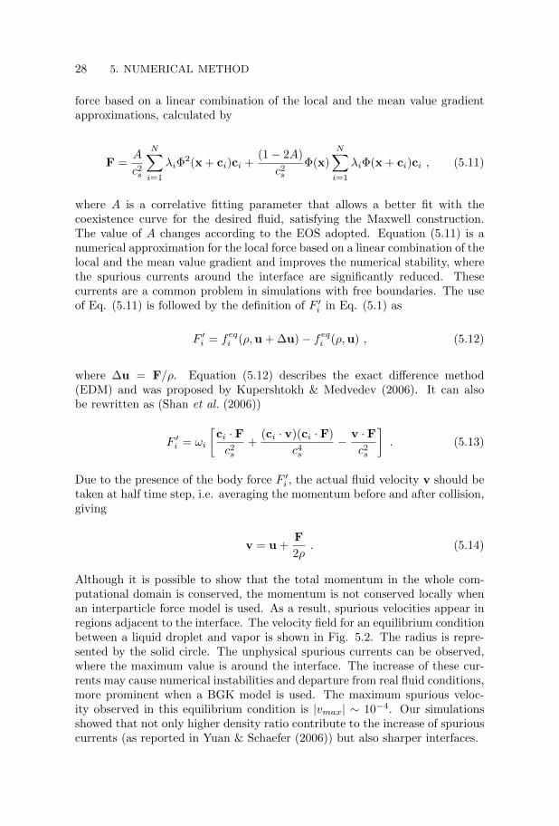
Although it is possible to show that the total momentum in the whole com-putational domain is conserved, the momentum is not conserved locally whenan interparticle force model is used. As a result, spurious velocities appear inregions adjacent to the interface. The velocity field for an equilibrium conditionbetween a liquid droplet and vapor is shown in Fig. 5.2. The radius is repre-sented by the solid circle. The unphysical spurious currents can be observed,where the maximum value is around the interface. The increase of these cur-rents may cause numerical instabilities and departure from real fluid conditions,more prominent when a BGK model is used. The maximum spurious veloc-ity observed in this equilibrium condition is |vmax| ∼ 10−4. Our simulationsshowed that not only higher density ratio contribute to the increase of spuriouscurrents (as reported in Yuan & Schaefer (2006)) but also sharper interfaces.

5.2. ENERGY EQUATION 29

0 20 40 60 80 1000

20

40

60

80

100

Figure 5.2. Velocity field for an equilibrium condition, whereTr = 0.85. The maximum velocity is |vmax| ∼ 10−4. Taken fromAlbernaz et al. (2013).

Through a Chapman-Enskog (C-E) analysis, the mass and momentum con-servation equations are obtained at the macroscopic scale, given respectivelyas (Chin (2001))

∂ρ

∂t+∇ · (ρv) = 0 , (5.15)

∂

∂t(ρv) +∇ · (ρvv) = −∇p+∇ · (2µS) + F′ , (5.16)

where µ is the dynamic viscosity and S = (∇v+(∇v)T )/2 the deviatoric stress.The pressure of the LBM is therefore calculated using an equation of state. Incontrast, in the direct numerical simulation of incompressible Navier-Stokesequations, the pressure satisfies a Poisson equation with velocity gradients act-ing as sources. Solving this equation for the pressure often produces numericaldifficulties that require special treatment. This has shown to be another ad-vantage of using LBM instead of conventional macroscopic methods.

5.2. Energy equation

The energy equation can be given in terms of the fluid temperature T . For aNewtonian fluid, this equation is given as (Bird (1960))

ρcvDT

Dt= ∇ · (k∇T )− T

(∂p

∂T

)ρ

∇ · u + µΦv , (5.17)

here cv is the specific heat at constant volume and k is the thermal conductivity.

30 5. NUMERICAL METHOD

The quantity Φv is known as the dissipation function and assumes, for athree-dimensional case,

Φv = 2

[(∂ux∂x

)2

+

(∂uy∂y

)2

+

(∂uz∂z

)2]

+

(∂uy∂x

+∂ux∂y

)2

+

(∂uz∂y

+∂uy∂z

)2

+

(∂ux∂z

+∂uz∂x

)2

− 2

3

(∂ux∂x

+∂uy∂y

+∂uz∂z

)2

(5.18)

Multiphase LBM have been used widely in isothermal flow simulations (e.g.Sbragaglia et al. (2009); Wagner & Yeomas (1999)). Recently, thermodynamiceffects with phase change have been considered in the LBM perspective bydifferent schemes (Gan et al. (2012)). Among the thermal LB models for mul-tiphase flows proposed, the multispeed (Gonnella et al. (2007)) and passivescalar (Zhang & Chen (2003)) approaches stand out. The multispeed approachassures energy conservation at a mesoscopic level, introducing the energy as amoment of distribution functions and enlarging the number of discrete speedsof the distribution functions in order to achieve the proper symmetries for theinternal energy flux. This approach comes with a higher computational cost.Throughout this work we use the passive scalar approach, where the tempera-ture field is advected passively by the fluid flow, so the coupling between energyand momentum is done at the macroscopic level. Moreover, this approach isnumerically more stable than the multispeed one.

By solving the temperature as a passive scalar, one can use the hybridscheme, where Eq. (5.17) is solved by finite difference scheme. In order to doso, Eq. (5.17) is rewritten with a forward Euler scheme as (Albernaz et al.(2016b))

T (x, t+ 1) = T (x, t)− v · ∇+T +1

ρcv∇+k∇+T + α∆+T

− T

ρcv

(∂p

∂T

)ρ

∇+ · v +ν

cvΦv , (5.19)

where α = k/(ρcv) denotes the thermal diffusivity and the superscript + corre-sponds to the finite difference operators. Equation (5.19) was used for solvingproblems where turbulence is considered (Papers 4 and 5). One could also solveEq. (5.17) by employing a double distribution function (DDF) scheme (Markus& Hazi (2011)) where a second distribution function is used for monitoring thetemperature field. This distribution can be given as

gi(x + ciδt, t+ δt) = gi(x, t)−1

τg(gi − geqi ) + Ci , (5.20)

5.3. VALIDATIONS AND TESTS 31

where Ci is a correction term and geqi denotes the equilibrium distributionfunction. The temperature is evaluated by

T =∑i

gi . (5.21)

The equilibrium function is written as

geqi = ωiT (1 + 3ci · v) . (5.22)

In order to obtain Eq. (5.17), the correction term Ci needs to assume

Ci = ωi

[∇ · (k∇T )

ρcv− αLB∇2T +

ν

cvΦv

]+ ωiT

[1− 1

ρcv

(∂p

∂T

)ρ

]∇ · v ,

(5.23)

where αLB = (τg − 1/2)/3 is the lattice thermal diffusivity.

5.3. Validations and tests

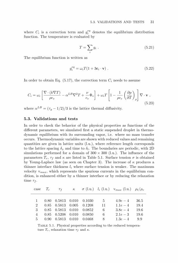
In order to check the behavior of the physical properties as functions of thedifferent parameters, we simulated first a static suspended droplet in thermo-dynamic equilibrium with its surrounding vapor, i.e. where no mass transferoccurs. Thermodynamic variables are shown with reduced values and remainingquantities are given in lattice units (l.u.), where reference length correspondsto the lattice spacing δx and time to δt. The boundaries are periodic, with 2Dsimulations performed for a domain of 300 × 300 (l.u.). The influence of theparameters Tr, τf and κ are listed in Table 5.1. Surface tension σ is obtainedby Young-Laplace law (as seen on Chapter 3). The increase of κ produces athinner interface thickness li where surface tension is weaker. The maximumvelocity vmax, which represents the spurious currents in the equilibrium con-dition, is enhanced either by a thinner interface or by reducing the relaxationtime τf .

case Tr τf κ σ (l.u.) li (l.u.) vmax (l.u.) ρ`/ρv

1 0.80 0.5813 0.010 0.1030 5 4.9e− 4 36.52 0.85 0.5813 0.005 0.1208 11 1.1e− 4 19.43 0.85 0.5813 0.010 0.0852 6 3.8e− 4 19.64 0.85 0.5208 0.010 0.0850 6 2.1e− 3 19.65 0.90 0.5813 0.010 0.0468 8 1.3e− 4 9.9

Table 5.1. Physical properties according to the reduced tempera-ture Tr, relaxation time τf and κ.

32 5. NUMERICAL METHOD

We observe that the density ratio ρ`/ρv is independent of τf , for the sameTr and κ. Furthermore, for lower values of τf the computational time needed toachieve equilibrium is raised. When Tr increases, for the same κ, the interface isthicker, which is expected as it gets closer to the critical point. It is importantto mention that these results were performed using a MRT collision operator.If a BGK model is employed to simulate the same static droplet with therelaxation times used in Table 5.1, the computations become unstable. Thedynamics of phase change had also to be validated, which is done by meansof a static radial droplet evaporation only due to diffusion. The analyticalsolution for the droplet evaporation rate obtained in section 2.3 is compared tothe numerical results.

In order to simulate a static droplet evaporation, the droplet is first equili-brated with the vapor at the saturated temperature in a periodic domain. Then,outflow boundaries are used, where Neumann boundary condition is applied tothe velocity. The temperature is then gently raised at the boundaries, set bya Dirichlet boundary condition. To keep the pressure p(ρ, T ) constant, densityis also set as DBC, calculated by the P-R EOS for a given initial pressure andcurrent temperature. The heat-up of the surrounding vapor, i.e. the conduc-tion of heat through the boundaries to the vapor phase toward the dropletinterface takes t ∼ 5×104. After this heat-up phase, the droplet evaporation isanalyzed. We observe that a symmetric radial flow is obtained, where no artifi-cial heating occurs. Consistent droplet evaporation was seen even for relativelyhigh density ratio, ρ`/ρv ∼= 130, for Tr = 0.7.

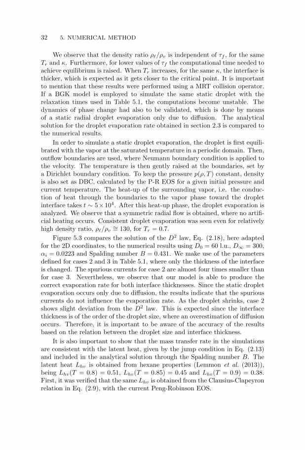
Figure 5.3 compares the solution of the D2 law, Eq. (2.18), here adaptedfor the 2D coordinates, to the numerical results using D0 = 60 l.u., D∞ = 300,αi = 0.0223 and Spalding number B = 0.431. We make use of the parametersdefined for cases 2 and 3 in Table 5.1, where only the thickness of the interfaceis changed. The spurious currents for case 2 are almost four times smaller thanfor case 3. Nevertheless, we observe that our model is able to produce thecorrect evaporation rate for both interface thicknesses. Since the static dropletevaporation occurs only due to diffusion, the results indicate that the spuriouscurrents do not influence the evaporation rate. As the droplet shrinks, case 2shows slight deviation from the D2 law. This is expected since the interfacethickness is of the order of the droplet size, where an overestimation of diffusionoccurs. Therefore, it is important to be aware of the accuracy of the resultsbased on the relation between the droplet size and interface thickness.

It is also important to show that the mass transfer rate in the simulationsare consistent with the latent heat, given by the jump condition in Eq. (2.13)and included in the analytical solution through the Spalding number B. Thelatent heat Lhv is obtained from hexane properties (Lemmon et al. (2013)),being Lhv(T = 0.8) = 0.51, Lhv(T = 0.85) = 0.45 and Lhv(T = 0.9) = 0.38.First, it was verified that the same Lhv is obtained from the Clausius-Clapeyronrelation in Eq. (2.9), with the current Peng-Robinson EOS.

5.3. VALIDATIONS AND TESTS 33

0 2 4 6 8 10

x 104

0.5

0.6

0.7

0.8

0.9

1

1.1

t

D2(t

)/D

02

κ=0.01 (case 3)

κ=0.005 (case 2)

D2 law

Figure 5.3. Normalized square diameter evolution in time, wherethe D2 law solution (Eq. (2.18)) and simulation results are shown,for two different interface thicknesses. Taken from Albernaz et al.

(2015).

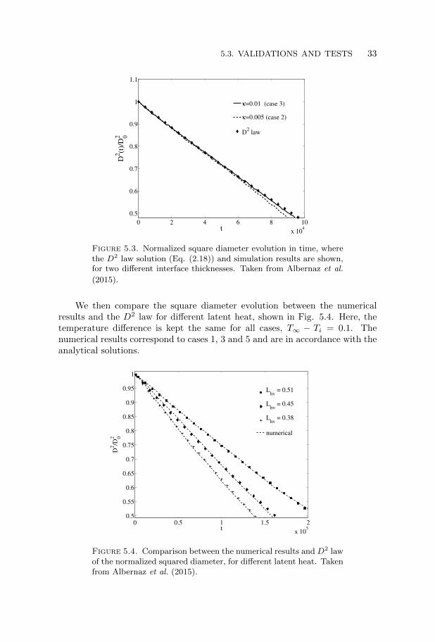
We then compare the square diameter evolution between the numericalresults and the D2 law for different latent heat, shown in Fig. 5.4. Here, thetemperature difference is kept the same for all cases, T∞ − Ti = 0.1. Thenumerical results correspond to cases 1, 3 and 5 and are in accordance with theanalytical solutions.

0 0.5 1 1.5 2

x 105

0.5

0.55

0.6

0.65

0.7

0.75

0.8

0.85

0.9

0.95

1

t

D2/D

02

Lhv

= 0.51

Lhv

= 0.45

Lhv

= 0.38

numerical

Figure 5.4. Comparison between the numerical results and D2 lawof the normalized squared diameter, for different latent heat. Takenfrom Albernaz et al. (2015).

34 5. NUMERICAL METHOD

It is seen that an increase of Lhv is responsible for a slower evaporation.Such behavior is expected, as more energy is needed to generate the phasechange. Figure 5.5 shows the relative error ε between the D2 law and nu-merical results as a function of the normalized square diameter. The error isevaluated at the same time-step. Different droplet sizes are tested, where theparameters used correspond to case 3 in Table 5.1. We note that good agree-ment with the D2 law is obtained, where the smaller droplet D0 = 50 givesε ∼= 1% when D2/D2

0 = 0.5.

0.50.60.70.80.910

0.2

0.4

0.6

0.8

1

ε (

%)

D2/D

0

2

D0 = 80

D0 = 60

D0 = 50

Figure 5.5. Error between D2 law and simulation results, for dif-ferent droplet sizes. Taken from Albernaz et al. (2015).

CHAPTER 6

Summary of results

We cover in this chapter the main results presented in Part II. Throughout thiswork we make use of a LBM method that incorporates phase change througha non-ideal equation of state, where a hexane fluid (C6H14) is considered.

6.1. Forced convection

Results from two-dimensional numerical simulations are reported in Albernazet al. (2013) and Albernaz et al. (2015), included as Paper 1 and Paper 2,respectively. Paper 1 deals mostly with model validation, where different equa-tions of state are considered. We observe that the Peng-Robinson EOS suitswell for describing a hexane fluid (as seen in Fig. 2.2). Static evaporationis analyzed, without imposing standard evaporation models (Sazhin (2006)),along with gravitational effects. In Paper 2 we have mainly focused on theanalysis of a convective flow around a droplet in a Lagrangian frame. We firsthave validated the latent heat and evaporation rate in our model by comparingit to the D2 law. The Reynolds number is based on the inlet velocity U anddroplet diameter D, assuming Re = UD/ν. We observe the droplet swellingcaused by the pressure wave due to the flow initialization. The saturated pres-sure in the whole domain is shifted by changing the inlet temperature untilan equilibrium condition is achieved, where no evaporation or condensationoccurs. The evaporation rate is then examined only by means of temperaturedifference between the incoming vapor and droplet, denoted as ∆T . Raisingthe superheated vapor temperature decreases the droplet lifetime, as expected.

The increase in Reynolds number can generate an oscillatory behavior inthe droplet. We analyze the droplet deformation based on a relation betweenthe droplet width and breadth. Due to the wake-droplet interactions, vorticesat the droplet bottom are periodically created and blown away, as shown inFig. 6.1. The solid circle denotes the droplet interface. First, (a) two symmet-ric eddies are formed at the droplet bottom region due to the flow separation,where the droplet deformation is maximum. The blowing along the droplet sur-face induces the detachment of these vortices (b), which are convected alongwith the vapor flow. The vortices develop and grow in size (c), and dropletdeformation reaches a minimum. A backflow is generated by these vortices(d), which assist the formation of new eddies close to the droplet bottom re-gion, completing an oscillatory cycle. Internal circulation is observed insidethe droplet. The evaporation rate is seen to increase also when convection is

35

36 6. SUMMARY OF RESULTS

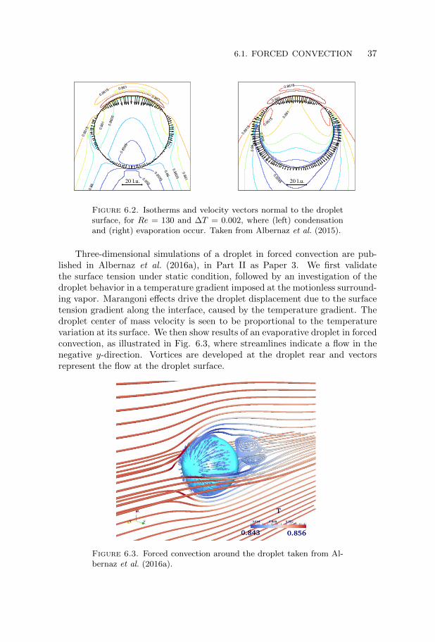
stronger, as the internal circulation enhances heat transfer. Figure 6.2 showsthe isotherms along with velocity vectors normal to the droplet surface at theonset of an evaporation case with ∆T = 0.002, where (left) condensation and(right) evaporation take place. A velocity vector pointing outwards means theoccurrence of local evaporation whereas if pointing inwards gives an indicationof local condensation. While Fig. 6.2 (left) shows condensation at the top andbottom regions, in (right) condensation happens only at the top, with strongerevaporation at the droplet sides. We show that a wider boundary layer (BL) isobtained due to this blowing as shear stresses around the droplet are decreased.We have also computed the velocity in tangential direction along the dropletsurface, which supports the effect of local blowing coupled to the BL thickness.

200 300

100

200

300

x

y

(a) (b)

(c) (d)

Figure 6.1. Streamlines for Re = 130 and ∆T = 0, taken fromAlbernaz et al. (2015).

6.1. FORCED CONVECTION 37

0.8

59

0.8

595

0.8

595

0.8

6

0.8

6

0.8

605

0.8

605

0.8

61

0.8

61

0.861

0.8

615

0.8615

0.862

20 l.u.

0.8

59

0.8

595

0.8

6

0.8

61

0.8

615

0.8

615

0.8615

0.862

20 l.u.

Figure 6.2. Isotherms and velocity vectors normal to the dropletsurface, for Re = 130 and ∆T = 0.002, where (left) condensationand (right) evaporation occur. Taken from Albernaz et al. (2015).

Three-dimensional simulations of a droplet in forced convection are pub-lished in Albernaz et al. (2016a), in Part II as Paper 3. We first validatethe surface tension under static condition, followed by an investigation of thedroplet behavior in a temperature gradient imposed at the motionless surround-ing vapor. Marangoni effects drive the droplet displacement due to the surfacetension gradient along the interface, caused by the temperature gradient. Thedroplet center of mass velocity is seen to be proportional to the temperaturevariation at its surface. We then show results of an evaporative droplet in forcedconvection, as illustrated in Fig. 6.3, where streamlines indicate a flow in thenegative y-direction. Vortices are developed at the droplet rear and vectorsrepresent the flow at the droplet surface.

Figure 6.3. Forced convection around the droplet taken from Al-bernaz et al. (2016a).

38 6. SUMMARY OF RESULTS

time ×105

0 0.5 1 1.5 2 2.5

D2

/D02

0.4

0.5

0.6

0.7

0.8

0.9

1

∆ T = 0.01

∆ T = 0.005

∆ T = 0.002

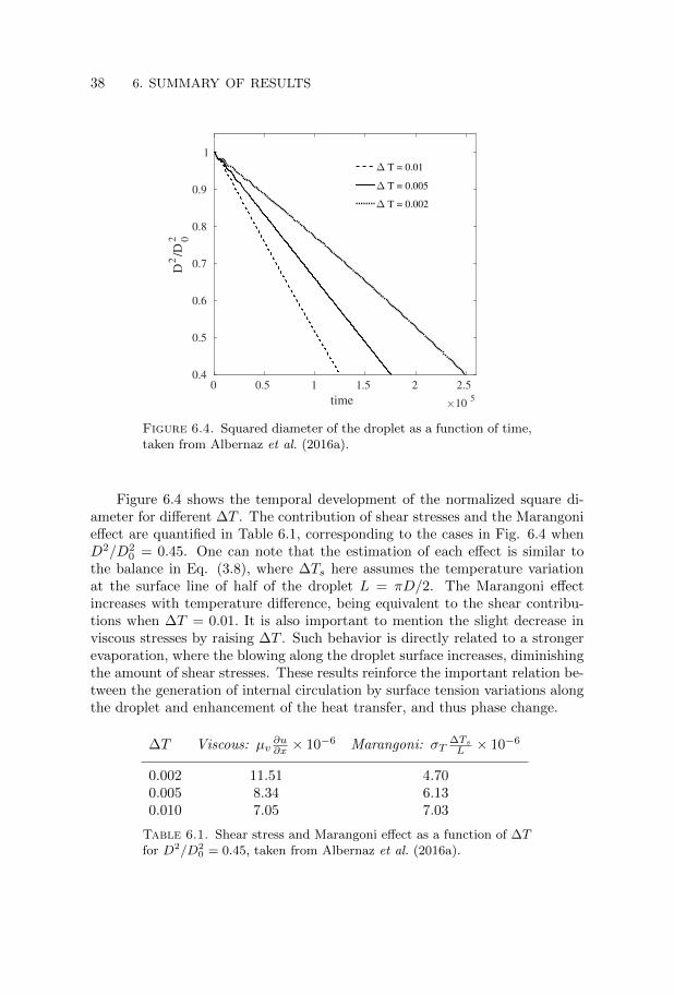
Figure 6.4. Squared diameter of the droplet as a function of time,taken from Albernaz et al. (2016a).

Figure 6.4 shows the temporal development of the normalized square di-ameter for different ∆T . The contribution of shear stresses and the Marangonieffect are quantified in Table 6.1, corresponding to the cases in Fig. 6.4 whenD2/D2

0 = 0.45. One can note that the estimation of each effect is similar tothe balance in Eq. (3.8), where ∆Ts here assumes the temperature variationat the surface line of half of the droplet L = πD/2. The Marangoni effectincreases with temperature difference, being equivalent to the shear contribu-tions when ∆T = 0.01. It is also important to mention the slight decrease inviscous stresses by raising ∆T . Such behavior is directly related to a strongerevaporation, where the blowing along the droplet surface increases, diminishingthe amount of shear stresses. These results reinforce the important relation be-tween the generation of internal circulation by surface tension variations alongthe droplet and enhancement of the heat transfer, and thus phase change.

∆T Viscous: µv∂u∂x × 10−6 Marangoni: σT

∆Ts

L × 10−6

0.002 11.51 4.700.005 8.34 6.130.010 7.05 7.03

Table 6.1. Shear stress and Marangoni effect as a function of ∆Tfor D2/D2

0 = 0.45, taken from Albernaz et al. (2016a).

6.2. TURBULENCE WITH A SINGLE PHASE FLUID 39

6.2. Turbulence with a single phase fluid

Extensive works for turbulent flows with an ideal EOS can be found for bothincompressible (Pumir 1994) and compressible cases (Kida & Orzag 1990). Ourcuriosity was raised when trying to answer the following question: what hap-pens for a real fluid in a turbulent flow when it assumes a temperature andpressure closer to the critical point? In order to answer this, we have analyzedin Albernaz et al. (2016b) (Paper 4) a single phase fluid in three-dimensionalisotropic turbulence. The fluid is described by a non-ideal EOS allowing usto scrutinize the difference of thermodynamic variables as conditions approachcriticality. Figure 6.5 shows the time evolution of temperature fluctuations forthe ideal EOS and different temperatures using the PR EOS. The fluctuationsare seen to increase with temperature. We have calculated and averaged anormalized pressure fluctuation based on the Reynolds decomposition, and ob-served fluctuations when T = 0.98 to be two orders of magnitude higher thanthe ones found for the ideal case.

t / tL

0 10 20 30 40

T′/T

×10-5

-10

-5

0

5

Ideal

T = 0.80

T = 0.90

T = 0.95

Figure 6.5. Turnover time evolution of the temperature fluctua-tions for Reλ ≈ 110, taken from Albernaz et al. (2016b).

The pressure PDF is shown in Fig. 6.6 for different temperatures. Theideal EOS result is also plotted and compared to data by Donzis & Jagan-nathan (2013), where good agreement is obtained. We have averaged the wholecomputational domain over multiple datasets, so that statistically robust infor-mation is ensured. For a PR EOS, the behavior for T = 0.8 resembles the idealcase. The enhancement of the temperature causes a decrease in the negativepressure fluctuations. While the negative tail narrows, the positive fluctuationseems to be insensitive to the temperature and follows a Gaussian distribu-tion (plotted as dotted lines). The PDFs for density and temperature are seen

40 6. SUMMARY OF RESULTS

to follow the same behavior. We have also analyzed the spectra of thermody-namic variables, where a Kolmogorov −5/3 scaling is obtained. A −7/3 scalingis observed for the pressure spectra in a narrow region of the inertial range,as reported both experimentally (Tsuji & Ishihara 2003) and numerically (Go-toh & Fukayama 2001). The kinetic energy spectra also shows a −5/3 scaling,where the spectrum is independent of the EOS or temperature considered.

p′/

√

p′2

-10 -5 0 5

log

10

PD

F

10-6

10-4

10-2

100

T = 0.98

T = 0.95

T = 0.90

T = 0.85

T = 0.80

Ideal

Figure 6.6. Semi-log pressure PDF for different temperatures.The dotted curve represents a Gaussian distribution, while datafor an Ideal EOS from Donzis & Jagannathan (2013) (circles) isalso plotted for comparison. Taken from Albernaz et al. (2016b).

We have also examined the effect of the Taylor Reynolds number on thethermodynamic fluctuations, as shown in Fig. 6.7. While the pressure fluc-tuations for the ideal case are insensitive to Reλ, the PR EOS shows a differ-ent scenario, where fluctuations increase significantly with Reλ for a conditionclose to the critical point. This unreported phenomena is more pronouncedwhen analyzing the skewness and flatness factors as a function of Reλ. Forall thermodynamic variables, the skewness (Fig. 6.8 (a)) is seen to increasewith Reλ, whereas flatness (Fig. 6.8 (b)) decreases with Reλ. This is a clearindication that the PDF of the thermodynamic fluctuations assume a behaviorcloser to a Gaussian distribution, where a narrower range of fluctuation is ob-tained. Therefore, we have found that the long negative tails seen for an idealfluid are not present with a non-ideal EOS when high temperature and Reλare considered.

6.3. DROPLET IN ISOTROPIC TURBULENCE 41

Reλ

50 100 150 200

1+p∗

0.998

0.9985

0.999

0.9995

1

Ideal

T = 0.80

T = 0.95

Figure 6.7. Pressure fluctuation for different Reλ, shown for theideal EOS and PR EOS. Taken from Albernaz et al. (2016b).

Reλ

80 120 160 200-1.3

-1.1

-0.9

-0.7

-0.5

Sp

Sρ

ST

(a)

Reλ

80 120 160 2003

4

5

6

7

Fp

Fρ

FT

(b)

Figure 6.8. (a) Skewness and (b) flatness factors for pressure, den-sity and temperature as a function of Reλ, with T = 0.95. Takenfrom Albernaz et al. (2016b).

6.3. Droplet in isotropic turbulence

We have also investigated in Albernaz et al. (2016c) (Paper 5) the dropletdynamics in a turbulent environment. The heat and mass transfer betweenphases are taken into consideration. This study is relevant to fuel sprays inenergy conversion systems as well as in nature, e.g. in the rain formation. Theprimary focus has been to analyze the coupling between turbulence parameters,

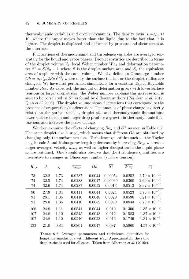
42 6. SUMMARY OF RESULTS

thermodynamic variables and droplet dynamics. The density ratio is ρ`/ρv ≈10, where the vapor moves faster than the liquid due to the fact that it islighter. The droplet is displaced and deformed by pressure and shear stress atthe interface.

Fluctuations of thermodynamic and turbulence variables are averaged sep-arately for the liquid and vapor phases. Droplet statistics are described in termsof the droplet volume Vd, local Weber number Wed and deformation parame-ter S∗ = S/S0 − 1, where S is the droplet surface area and S0 the equivalentarea of a sphere with the same volume. We also define an Ohnesorge numberOh = µ`/(ρ`2Rσ)1/2, where only the surface tension or the droplet radius arechanged. We have first performed simulations for a constant Taylor Reynoldsnumber Reλ. As expected, the amount of deformation grows with lower surfacetensions or larger droplet size: the Weber number explains this increase and isseen to be correlated to S∗ as found by different authors (Perlekar et al. 2012;Qian et al. 2006). The droplet volume shows fluctuations that correspond to thepresence of evaporation/condensation. The amount of phase change is directlyrelated to the surface tension, droplet size and thermodynamic fluctuations:lower surface tension and larger drop produce a growth in thermodynamic fluc-tuations and increase the phase change.

We then examine the effects of changing Reλ and Oh as seen in Table 6.2.The same droplet size is used, which means that different Oh are obtained bychanging only the surface tension. Turbulence quantities such as the Taylorlength scale λ and Kolmogorov length η decrease by increasing Reλ, whereas alarger averaged velocity urms as well as higher dissipation in the liquid phaseε` are obtained. One should also observe that the turbulence quantities areinsensitive to changes in Ohnesorge number (surface tension).

Reλ λ η urms Oh S∗ Wed ε`

73 32.2 1.73 0.0287 0.0044 0.00054 0.0252 2.79× 10−10

74 32.5 1.74 0.0288 0.0047 0.00069 0.0300 2.69× 10−10

74 32.6 1.74 0.0287 0.0052 0.0013 0.0512 3.32× 10−10

90 27.9 1.34 0.0411 0.0044 0.0024 0.0523 5.76× 10−10

91 28.1 1.35 0.0410 0.0048 0.0029 0.0596 5.21× 10−10

91 28.0 1.35 0.0410 0.0052 0.0049 0.0843 5.79× 10−10

106 24.8 1.11 0.0541 0.0044 0.010 0.1306 1.35× 10−9

107 24.8 1.10 0.0545 0.0048 0.012 0.1583 1.37× 10−9

107 24.8 1.10 0.0546 0.0053 0.016 0.1749 1.31× 10−9

133 21.0 0.84 0.0801 0.0047 0.087 0.5960 4.57× 10−9

Table 6.2. Averaged parameters and turbulence quantities forlong-time simulations with different Reλ. Approximately the samedroplet size is used for all cases. Taken from Albernaz et al. (2016c).

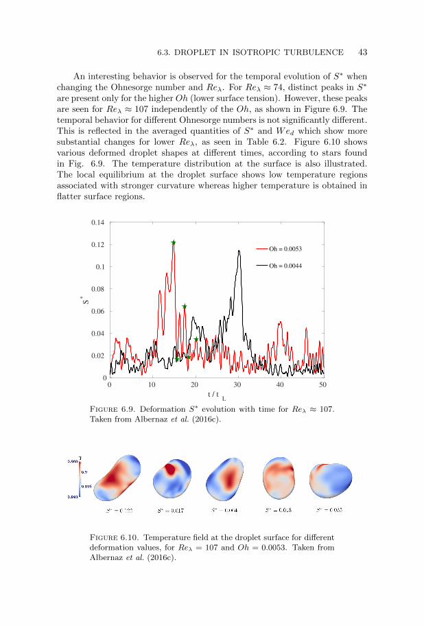
6.3. DROPLET IN ISOTROPIC TURBULENCE 43

An interesting behavior is observed for the temporal evolution of S∗ whenchanging the Ohnesorge number and Reλ. For Reλ ≈ 74, distinct peaks in S∗

are present only for the higher Oh (lower surface tension). However, these peaksare seen for Reλ ≈ 107 independently of the Oh, as shown in Figure 6.9. Thetemporal behavior for different Ohnesorge numbers is not significantly different.This is reflected in the averaged quantities of S∗ and Wed which show moresubstantial changes for lower Reλ, as seen in Table 6.2. Figure 6.10 showsvarious deformed droplet shapes at different times, according to stars foundin Fig. 6.9. The temperature distribution at the surface is also illustrated.The local equilibrium at the droplet surface shows low temperature regionsassociated with stronger curvature whereas higher temperature is obtained inflatter surface regions.

0 10 20 30 40 50

t / tL

0

0.02

0.04

0.06

0.08

0.1

0.12

0.14

S*

Oh = 0.0053

Oh = 0.0044

Figure 6.9. Deformation S∗ evolution with time for Reλ ≈ 107.Taken from Albernaz et al. (2016c).

Figure 6.10. Temperature field at the droplet surface for differentdeformation values, for Reλ = 107 and Oh = 0.0053. Taken fromAlbernaz et al. (2016c).

44 6. SUMMARY OF RESULTS

The oscillation frequency of the droplet has been investigated and comparedto classical predictions by Rayleigh (1879). The basic modes of oscillation n = 2and n = 3 could be identified for Reλ = 74 (Fig. 6.11). However, for Reλ = 107as shown in Fig. 6.12, these modes are not distinct. Instead, they are replacedby a continuous spectrum, showing a decrease that scales as ∼ f−3.

10-1

100

101

f

10-8

10-7

10-6

10-5

10-4

10-3

|S∗−

S∗|

Oh = 0.0052

Oh = 0.0044

Figure 6.11. Power spectrum of the deformation parameter as afunction of frequency for Reλ = 74. The theoretical basic modes ofoscillation are represented by solid lines (Oh = 0.0052) and dashedlines (Oh = 0.0044). Taken from Albernaz et al. (2016c).

10-1

100

101

f

10-8

10-7

10-6

10-5

10-4

10-3

|S∗−

S∗|

Oh = 0.0053

Oh = 0.0044

f-3

Figure 6.12. Power of the deformation parameter for Reλ = 107,taken from Albernaz et al. (2016c).

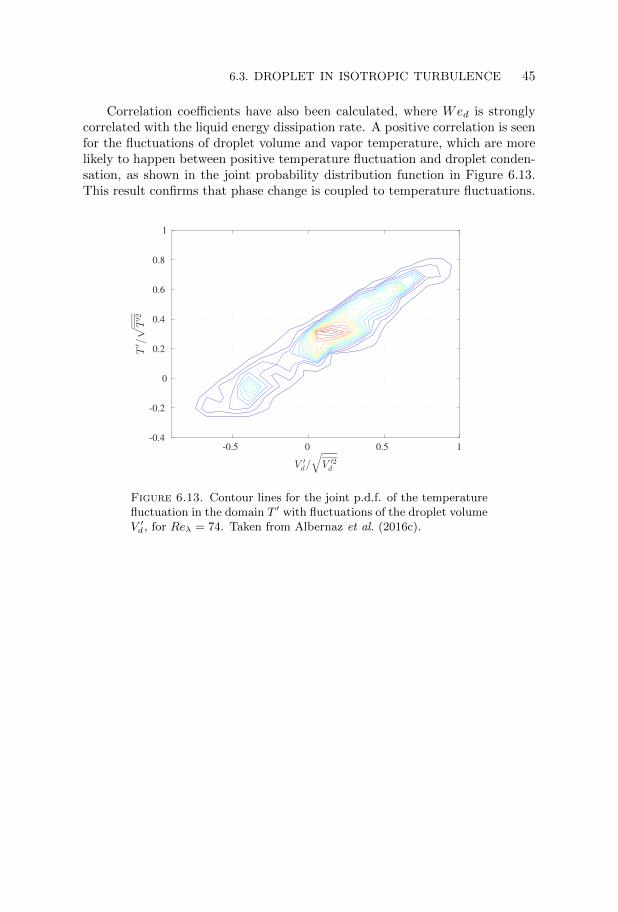
6.3. DROPLET IN ISOTROPIC TURBULENCE 45

Correlation coefficients have also been calculated, where Wed is stronglycorrelated with the liquid energy dissipation rate. A positive correlation is seenfor the fluctuations of droplet volume and vapor temperature, which are morelikely to happen between positive temperature fluctuation and droplet conden-sation, as shown in the joint probability distribution function in Figure 6.13.This result confirms that phase change is coupled to temperature fluctuations.

-0.5 0 0.5 1

V ′

d/

√

V ′2

d

-0.4

-0.2

0

0.2

0.4

0.6

0.8

1

T′/√

T′2

Figure 6.13. Contour lines for the joint p.d.f. of the temperaturefluctuation in the domain T ′ with fluctuations of the droplet volumeV ′d , for Reλ = 74. Taken from Albernaz et al. (2016c).

CHAPTER 7

Concluding remarks

We have investigated the dynamics of an evaporative droplet under static con-ditions and forced convection. Unlike standard numerical approaches, wherethe interactions between different phases need to be described with appro-priate jump conditions, we control the phase change directly by a non-idealequation of state. This is possible by using a mesoscopic lattice Boltzmannmethod. We have first validated the evaporation rate and latent heat with atheoretical evaporation prediction, known as the D2 law. An advantage of theabsence of assumptions, such as constant surface tension forces and droplettemperature, resides in highlighting phenomena that are usually neglected,such as Marangoni forces. Under certain conditions, we have observed thatthe Marangoni effect plays a major role.

We have also used this model to study flows in isotropic turbulence. Thenovelty in using a non-ideal equation of state to establish local thermodynamicproperties has led us to examine a single phase fluid approaching the criticalpoint. Unreported phenomena have been revealed based on detailed analyses ofthermodynamic variables behavior and different turbulent intensities. Lastly,we have investigated the dynamics of a droplet in turbulence. The heat andmass transfer, as well as the density contrast are considered. To the best of theauthors’ knowledge, such conditions have not been previously treated. Strongcorrelations between droplet deformation, volume fluctuations due to phasechange occurrence and temperature fluctuations have been reported. We havealso looked into the temporal spectra of droplet deformations coupled to thedroplet oscillatory modes.

The main contribution of this work lies in the possibility of studying realfluids in both evaporative and turbulent environments. A spontaneous continu-ation of this work would be the inclusion of a multicomponent model. Instead ofanalyzing the droplet surrounded by its own vapor, the insertion of a gas wouldallow the study of other parameters such as the diffusion coefficient and massfraction of different species. This improvement would bring the model closerto available experimental data, allowing its validation by a direct comparison.

Another suggestion for future work would be the investigation of dropletcollisions surrounded by a gas with higher temperature. The primary focuswould be on how phase change can affect droplet interactions. It would beinteresting to consider a wide range of surface tension variation, which rightnow is a limitation to the present model: surface tension is not an independent

46

7. CONCLUDING REMARKS 47

variable. Publications using lattice Boltzmann methods applied to multiphaseflows have increased substantially over the last five years, where new modelsand approaches are opening doors to broaden applicability. A remedy to thesurface tension might be found in a recent work by Xu et al. (2015), wheresurface tension can be tuned in order to assume a desirable value.

Further on, a similar model could also be used for simulating the breakup ofa jet injected in a hot gas flow. As breakup is spontaneously included based onlocal thermal properties, several scales could be studied in detail without the useof modelling, as currently done by standard computational fluid dynamics. Thiswould shed more light on how to optimize conditions for achieving homogeneityof the mixture of the fuel and the surrounding air. One would aim for aparameter investigation by changing properties such as surface tension anddensity ratio. The use of multicomponent models would allow investigations ofthe effect of additives in the fuel, with direct application to biodiesel fuels.

Acknowledgements

First of all I would like to express my gratitude to my supervisor Prof. GustavAmberg. I am thankful for the opportunity of coming to Sweden, a country Ilearned to love, and for being his PhD student. It has been a pleasure workingwith Gustav, he always has something to contribute, either by insights or simplyby motivation and positive attitude. Gustav is a kind person with a deepphysical knowledge that spreads good energy independently of how well orbad things are. A big thanks to my co-supervisor Minh Do-Quang for hispatience and for many fruitful discussions. Without his amazing knowledge inprogramming, this thesis would not have been possible.

I am grateful to my academic father and friend Prof. Francisco Ricardo(University of Brasilia) for his endless help and for sharing his passion forscience. Thanks for introducing me to Fluid dynamics and all its differentnuances. I would also like to acknowledge contributions to this work from Prof.Jim Hermanson (University of Washington).

Special thanks to my everyday office mates, former and actual ones: Yuli,Andreas, Zeinab, Amer, Timea and Abdul-Malik. I have to thank los cabronesfor the good times we had and will surely keep having, Ricardo, Ramin, Pau,George, Werner, Sasan, Maffioli, Freddy, Walter, Jacopo, Prabal and Luis.Jag tackar ocksa all personal fran avdelningen: ni har varit sa hjalpsamma,sarskilt Heide, Carolina, Malin och Bubba.

Along this journey I am glad to have met so many people which madeMechanics such a nice environment, I would like to thank you all: Enrico,Stevin, Bernard, Karl, Lailai, Sohrab, Ferro, Azad, Lukas, Matteo, Alex, Yuki,Alexandra, Ashwin, Geert, Elektra, Tomas, Shervin, Ugis, Nima, Iman, Armin,Erik, Priti, Ekaterina, Jiewei, Mehdi, Mireia, Igor, Emanuele, Mattias, Nicolas,Taras, Brandt, Biancofore, Gaetano, Picano and others which I might haveforgotten to include. That’s what happens when you leave this part to bewritten last.

And talking about last, but not least, my deepest gratitude to my family.Mamadinha and Vanessa, you have always been there, encouraging and sup-porting me. Sou eternamente grato! I have so much luck in my life for havingyou and for having my sambo Fannie: tack alskling for ditt stod och for allkarlek som du ger mig: du ar min gladje!

49

Bibliography

Albernaz, D. L., Do-Quang, M. & Amberg, G. 2013 Lattice boltzmann methodfor the evaporation of a suspended droplet. Interfac. Phenom. Heat Transfer 1,245–258.

Albernaz, D. L., Do-Quang, M. & Amberg, G. 2015 Multirelaxation-time latticeboltzmann model for droplet heating and evaporation under forced convection.Phys. Rev. E 91, 043012.

Albernaz, D. L., Amberg, G. & Do-Quang, M. 2016a Simulation of a suspendeddroplet under evaporation with Marangoni effects. accepted for publication inInt. J. Heat Mass Transf .

Albernaz, D. L., Do-Quang, M., Hermanson, J. C. & Amberg, G. 2016b Realfluids near the critical point in isotropic turbulence. under revision in Phys.Fluids.

Albernaz, D. L., Do-Quang, M., Hermanson, J. C. & Amberg, G. 2016cDroplet deformation and heat transfer in isotropic turbulence. submitted to J.Fluid Mech..

Balaji, B. Raghavan, V., Ramamurthi, & Gogos, K.G. 2011 A numerical studyof evaporation characteristics of spherical n-dodecane droplets in high pressurenitrogen environment. Phys. Fluids 23, 063601.

Banerjee,R. 2013 Numerical investigation of evaporation of a single ethanol/iso-octane droplet. Fuel 107, 724–739.

Bird, R. B. 1960 Transport Phenomena. John Wiley & Sons, New York.

Bhatnagar, P. L., Gross, E. P. & Krook, M. 1954 Model for collision processesin gases. Phys. Rev. 94, 511–525.

Borg, A., Bolinder J. & Fuchs, L. 2001 Simultaneous velocity and concentrationmeasurements in the near-field of a turbulent low-pressure jet by DPIV-PLIFregion of a turbulent jet flow. Exp. in Fluids 31, 140–152.

Chen, S. & Doolen, G. D. 1998 Lattice boltzmann method for fluid flows. Annu.Rev. Fluid Mech. 30, 329–364.

Chin, J. 2001 Mesoscale modelling with the Lattice Boltzmann Method. University ofLondon.

Dec, J. E. 1997 A conceptual model of DI diesel combustion based on laser-sheetimaging. SAE Paper , 970873.

Donzis, D. A. & Jagannathan, S. 2013 Fluctuations of thermodynamic variablesin stationary compressible turbulence. J. Fluid Mech. 733, 221–244.

50

BIBLIOGRAPHY 51

Erbil, H. Y. 2012 Evaporation of pure liquid sessile and spherical suspended drops:A review. Adv. Colloid Interface Sci. 170, 67–86.

Faghri, A. & Zhang, Y. 2006 Transport phenomena in multiphase systems. Elsevier,Oxford.

Gan, Y., Xu, A., Zhang, G., Zhang, P. & Li, Y. 2012 Lattice boltzmann studyof thermal phase separation: Effects of heat conduction, viscosity and prandtlnumber. EPL 97, 44002.

Gonnella, G., Lamura, A. & Sofonea, V. 2007 Lattice boltzmann simulation ofthermal nonideal fluids. Phys. Rev. E 76, 036703.

Gorokhovski, M. & Herrmann, M. 2007 Modelling Primary Atomization. Annu.Rev. Fluid Mech. 40, 343–366.

Gotoh, T. & Fukayama, D. 2001 Pressure spectrum in homogeneous turbulence.Phys. Rev. Lett. 86, 1775–3778.

Grigoriev, I. G., Wallin, S. W., Brethouwer, G. B. & Johansson, A. V. J.2013 A realizable explicit algebraic Reynolds stress model for compressible tur-bulent flow with significant mean dilatation. Phys. Fluids 25, 105112.

Guillard, F., Fritzon, R., Revstedt, J., Tragardh, C., Alden, M. & Fuchs,L. 1998 Mixing in a confined turbulent impinging jet using planar laser inducedfluorescence. Exp. in Fluids 25, 143–150.

Guyon, E., Hulin, J.-P., Petit, L. & Mitescu, C. D. 2001 Physical hydrodynam-ics. University Press, Oxford.

Hase, M. & Weigand, B. 2004 Transient heat transfer of deforming droplets at highreynolds numbers. Int. J. Numer. Methods Heat Fluid Flow 14, 85–97.

He, X. & Doolen, G. D. 2002 Thermodynamic foundations of kinetic theory andlat- tice Boltzmann models for multiphase flows. J. Stat. Phys. 107, 309–328.

Holyst, R., Litniewski, M., Jakubczyk, D., Kolwas, K. & Kolwas, M. 2013Evaporation of freely suspended single droplets: experimental, theoretical andcomputational simulations. Rep. Prog. Phys. 76, 034601.

Ishihara, T., Gotoh, T. & Kaneda, Y. 2009 Study of high–reynolds numberisotropic turbulence by direct numerical simulation. Annu. Rev. Fluid Mech. 41,165–180.

Jiang, S., Siamas, G. A., Jagus, K. & Karayiannis, T. G. 2010 Physical mod-elling and advanced simulations of gas-liquid two-phase jet flows in atomizationand sprays. Progress in Energy and Combustion Science 36, 131–167.

Kaplun, A.B. & Meshalkin, A.B. 2003 Thermodynamic validation of the form ofunified equation of state for liquid and gas, High Temperature 41, 319-326.

Kekesi, T., Gustav, A. & Wittberg, L. P. 2014 Drop deformation and breakup.Int. J. Multiphase Flow 66, 1–10.

Kida, S. &Orzag, S. A. 1990 Energy and spectral dynamics in forced compressibleturbulence. J. Sci. Comput. 5, 85–125.

Kolmogorov, A. N. 1994a The local structure of turbulence in incompressible vis-cous fluid for very large Reynolds numbers [In Russian]. Dokl. Akad. Nauk SSSR30, 299–301.

Kolmogorov, A. N. 1994b Dissipation of energy in locally isotropic turbulence [InRussian]. Dokl. Akad. Nauk SSSR 32, 19–21.

52 BIBLIOGRAPHY

Kuo, K. K. Y. 2005 Principles of Combustion. John Wiley & Sons, New York.

Kupershtokh, A. L. & Medvedev, D. A. 2006 Lattice boltzmann equation methodin electrohydrodynamic problems. J. Electrostat. 64, 581–585.

Kupershtokh, A. L., Medvedev, D. A. & Karpov, D. I. 2009 On equations ofstate in a lattice boltzmann method. Comput. Math. Appl. 58, 965–974.

Lallemand, P. & Luo, L. S. 2000 Theory of the lattice boltzmann method: Dis-persion, dissipation, isotropy, galilean invariance, and stability. Phys. Rev. E 61,6546.

Lasheras, J. C., Villermaux, E. & Hopfinger, E. J. 1998 Break-up and atom-ization of a round water jet by a high-speed annular air jet. J. Fluid. Mech. 357,351–379.

Lefebvre, A. H. 1989 Atomization and sprays. Taylor & Francis, Bristol.

Levich, V. G. 1962 Physicochemical hydrodynamics. Englewood Cliffs, N.J.:Prentice-Hall.

Marangoni, C. G. M. 1871 Ueber die ausbreitung der tropfen einer flussigkeit aufder oberflache einer anderen. Ann. Phys. Chem. 143, 337–354.

Markus, A. & Hazi, G. 2011 Simulation of evaporation by an extension of thepseudopotential lattice boltzmann method: A quantitative analysis. Phys. Rev.E 83, 046705.

Lemmon, E.W., McLinden, M.O. & Friend, D.G. 2013 Thermophysical Proper-ties of Fluid Systems. In NIST Chemistry WebBook, NIST Standard ReferenceDatabase Number (ed. Linstrom P.J. & Mallard W.G.), vol. 69. National Instituteof Standards and Technology, Gaithersburg MD.

Perlekar, P., Biferale, L., Sbragaglia, M., Srivstava, S. & Toschi, F. 2012Droplet size distribution in homogeneous isotropic turbulence. Phys. Fluids 24,065101.

Pope, S. B. 2000 Turbulent flows. Cambridge University Press, Cambridge.

Probstein, R. F. 1994 Physicochemical hydrodynamics: an introduction. John Wiley& Sons, New York.

Pumir, A. 1994 A numerical study of pressure fluctuations in three-dimensional,incompressible, homogeneous, isotropic turbulence. Phys. Fluids 6, 2071–2083.

Qian, D., McLaughlin, J. B., Sankaranarayanan, K., Sundaresan, S. & Kon-tomaris, K. 2006 Simulation of bubble breakup dynamics in homogeneous tur-bulence. Chem. Eng. Comm. 193, 1038–1063.

Reynolds, O. 1895 On the dynamical theory of incompressible viscous fluids and thedetermination of the criterion. Philos. Trans. Roy. Soc. London 186, 123–164.

Rayleigh, Lord 1879 On the capillary phenomena of jets. Proc. R. Soc. London 29,71–97.

Rayleigh, Lord 1883 Investigation of the character of the equilibrium of an incom-pressible heavy fluid of variable density. Proc. London Math. Soc. 14, 170–177.

Richardson, L. F. 1922 Weather Prediction by Numerical Process. Dover Publica-tions, Inc., New York.

Safari, H., Rahimian, M. H. & Krafczyk, M. 2013 Extended lattice boltzmannmethod for numerical simulation of thermal phase change in two-phase fluid flow.Phys. Rev. E 88, 013304.

BIBLIOGRAPHY 53

Sazhin, S. S. 2006 Advanced models of fuel droplet heating and evaporation. Prog.Energy Combust. Sci. 32, 162–214.

Sbragaglia, M., Benzi, R., Biferale, L., Chen, H., Shan, X. & Succi, S. 2009Lattice boltzmann method with self-consistent thermo-hydrodynamic equilibria.J. Fluid Mech. 628, 299–309.

Scardovelli, R. & Zaleski, S. 1999 Direct numerical simulation of free-surfaceand interfacial flow. Annu. Rev. Fluid Mech. 31, 567–603.

Schlottke, J. & Weigand, B. 2008 Direct numerical simulation of evaporatingdroplets. J. Comput. Phys. 227, 5215–5237.

Sedarsky, D., Berrocal, E. & Linne, M. 2008 Ballistic imaging for measurementof flow structures in dense multiphase media. 14th International Symposium onApplications of Laser Techniques to Fluid Mechanics.

Sethian, J. A. & Smereka, P. 2003 Level set methods for fluid interfaces. Annu.Rev. Fluid Mech. 35, 341–372.

Shan, X. & Chen, H. 1993 Lattice boltzmann model for simulating flows withmultiple phases and components. Phys. Rev. E 47, 1815.

Shan, X. & Chen, H. 1994 Simulation of nonideal gases and liquid-gas phasetransitions by the lattice Boltzmann equation. Phys. Rev. E 49, 2941.

Shan, X., Yuan, X. F. & Chen, H. 2006 Kinetic theory representation of hydrody-namics: a way beyond navier-stokes equation. J. Fluid Mech. 550, 413–441.

Shi, Y., Ge, H.-W. & Reitz, R. D. 2011 Computational Optimization of InternalCombustion Engines. Springer-Verlag, London.

Shinjo, J. & Umemura, A. 2010 Simulation of liquid jet primary breakup: Dynamicsof ligament and droplet formation. Int. J. Multiphase Flow 36, 513–532.

Shinjo, J. & Umemura, A. 2011 Detailed simulation of primary atomization mech-anisms in Diesel jet sprays (isolated identification of liquid jet tip effects) Proc.Combust. Inst. 33, 2089–2097.

Sirignano, W. A. 2010 Fluid Dynamics and Transport of Droplets and Sprays. Cam-bridge University Press, Cambridge.

Strotos, G., Gavaises, M., Theodorakakos, A. & Bergeles, G. 2011 Nu-merical investigation of the evaporation of two-component droplets. Fuel 90,1492–1507.

Sukop, M.C. & Thorne, D.T. 2006 Lattice Boltzmann modelling: an introductionfor geoscientists and engineers. Berlin: Springer.

Taylor, C. F. 1985 The internal-combustion engine in theory and practice. MITPress, Cambridge.

Tanguy, S., Menard, T. & Berlemont, A. 2007 A level set method for vapor-izing two-phase flows. J. Comput. Phys. 221, 837–853.

Tryggvason, G., Brunner, B., Esmaeeli, A., Juric, D., Al-Rawahi, N.,Tauber, W., Han, J., Nas, S. & Jan, Y.-J. 2001 A front-tracking methodfor the computations of multiphase flow. J. Comput. Phys. 169, 708–759.

Tsuji, Y. & Ishihara, T. 2003 Similarity scaling of pressure fluctuation in turbu-lence. Phys. Rev. E 68, 026309.

Wagner, A. J. & Yeomas, J. M. 1999 Phase separation under shear in two-dimensional binary fluids. Phys. Rev. E 59, 4366–4373.

Xu, A., Tao, T. S., An, L. & Shi, L. 2015 A three-dimensional pseudo-potential-based lattice Boltzmann model for multiphase flows with large density ratio andvariable surface tension. Int. J. Heat Fluid Flow 56, 261–271.

P. Yuan, & Schaefer, L. 2006 Equations of state in a lattice Boltzmann model,Phys. Fluids 18, 042101.

Zhang, H. 2003 Evaporation of a suspended droplet in forced convective high-pressure environments. Combust Sci. and Tech. 175, 2237–2268.

Zhang, R. & Chen, H. 2003 Lattice boltzmann method for simulations of liquid-vapor thermal flows. Phys. Rev. E 67, 066711.