damage diagnosis of algorithms for wireless structural
TRANSCRIPT

Department of Civil and Environmental Engineering
Stanford University
Report No. 165 November 2007
Damage Diagnosis of Algorithms for Wireless Structural Health Monitoring
By
Krishnan Nair Kesavanand Anne S. Kiremidjian

The John A. Blume Earthquake Engineering Center was established to promote research and education in earthquake engineering. Through its activities our understanding of earthquakes and their effects on mankind’s facilities and structures is improving. The Center conducts research, provides instruction, publishes reports and articles, conducts seminar and conferences, and provides financial support for students. The Center is named for Dr. John A. Blume, a well-known consulting engineer and Stanford alumnus.
Address:
The John A. Blume Earthquake Engineering Center Department of Civil and Environmental Engineering Stanford University Stanford CA 94305-4020
(650) 723-4150 (650) 725-9755 (fax) [email protected] http://blume.stanford.edu
©2007 The John A. Blume Earthquake Engineering Center

ii
Abstract
Recent research efforts in wireless structural health monitoring have resulted in an
explosion in the development of new sensors. Little attention, however, has been focused
on the efficient and effective use of the data collected by these sensors. While these
wireless sensor networks enable dense instrumentation, the amount of data that needs to
be transmitted can prove to be prohibitive. The main difficulty arises from the low data
rates associated with low power ad-hoc wireless sensor networks. Thus, data transmission
over the wireless network is demanding, time consuming and can significantly reduce
power source life. Typically these data are required because current damage detection
algorithms perform global system level analysis rather than local sensor level analysis. In
this dissertation, three local sensor based damage diagnosis algorithms using statistical
signal processing and pattern classification techniques have been developed. The main
features of these algorithms are that they are simple, robust and computationally efficient.
The first algorithm uses time series to model the vibration signal and defines a damage
sensitive feature DSF using the first three autoregressive (AR) coefficients. A t-test on
the DSF’s is used to discriminate between an undamaged state and a damaged state. This
algorithm is valid for linear and stationary signals.
The second algorithm utilizes the first three AR coefficients as the feature vector.
Damage detection is performed using the Gaussian Mixture Models (GMM’s) and the
gap statistic. This algorithm, like the first algorithm described above, is valid for linear,

iii
stationary signals. This algorithm is shown to be more effective in detecting minor
damage patterns in comparison to the first algorithm. A damage measure has been
developed using the Mahalanobis distance between the means of the damaged and
undamaged datasets.
The third algorithm uses the wavelet energies at the fifth, sixth and seventh dyadic scales
as feature vectors. This algorithm allows the use of non-stationary signals. This algorithm
requires a creation of a database of baseline signals. The first part of this algorithm
requires finding that signal in the database closest to the new signal. The second part of
this algorithm is to obtain the feature vectors. Both of these steps are performed using
principal components analysis. Damage detection is performed using the k-means
algorithm in conjunction with the gap statistic. A damage measure has been developed
using the Euclidean distance between the means of the damaged and undamaged feature
vector.
The performance of the developed algorithms is validated using the datasets of the ASCE
Benchmark Structure. It is observed that the damage patterns as defined in the ASCE
Benchmark Structure are consistently identified using these algorithms. The damage
measures are also shown to correlate well with the extent of damage.

iv
Acknowledgments
This research was supported in part by the John A. Blume Research Fellowship, the
National Science Foundation Grant No. CMS-0121841, the National Science Foundation
- George E. Brown, Jr. Network for Earthquake Engineering Simulation Research Grant
No. 15BBK16379 and by the John A. Blume Earthquake Engineering Research Center.

v
Table of Contents
Abstract ii
Acknowledgments iv
List of Tables viii
List of Figures ix
1 Introduction 1
1.1 Motivation .........................................................................................................1
1.2 Objectives..........................................................................................................6
1.3 Organization of the Thesis ................................................................................6
2 A Time Series Based Damage Detection Algorithm with Hypothesis Testing 8
2.1 Description of the Damage Detection Algorithm .............................................9
2.1.1 Modeling of the Vibration Signals ........................................................10
2.1.2 Development of Damage Sensitive Feature (DSF) ...............................17
2.1.3 Correlation of the AR Coefficients to the Structural System ................18
2.2 Damage Detection Algorithm Synthesis .........................................................24
2.3 Application Results .........................................................................................25
2.3.1 Damage Detection .................................................................................28
2.4 Summary .........................................................................................................33
3 A Time Series Based Structural Damage Detection Algorithm Using
Gaussian Mixture Modeling 37
3.1 Overview of the Damage Diagnosis Algorithm ..............................................38

vi
3.2 Modeling of Vibration Signals ........................................................................40
3.3 Gaussian Mixture Modeling ...........................................................................41
3.4 Damage Diagnosis using Gaussian Mixture Models ......................................45
3.4.1 Damage Identification using the Gap Statistic ......................................45
3.5 Damage Extent using the Mahalanobis Metric ...............................................47
3.6 Application ......................................................................................................48
3.6.1 Damage Detection .................................................................................48
3.6.2 Damage Extent ......................................................................................56
3.6.3 Effect of Noise on the Damage Diagnosis.............................................58
3.7 Summary .........................................................................................................60
3.8 Appendix: The EM Algorithm ........................................................................61
4 Damage Feature Extraction from Wavelet Transform of Vibration Signals 65
4.1 Properties of the Continuous Wavelet Transform...........................................66
4.1.1 Haar Wavelet .........................................................................................69
4.1.2 Morlet Wavelet ......................................................................................70
4.2 Derivation of the Damage Sensitive Feature using Wavelet Coefficients
of Acceleration Signals for a SDOF System ...................................................71
4.2.1 Wavelet Transform of Acceleration Signals .........................................74
4.2.1.1 Haar Wavelet Coefficients of Acceleration Signals ................74
4.2.1.2 Morlet Wavelet Coefficients of Acceleration Signals .............75
4.2.2 Damage Sensitive Feature .....................................................................77
4.2.2.1 Haar Basis ................................................................................77
4.2.2.2 Morlet Basis ............................................................................79
4.3 Derivation of the Damage Sensitive Feature using Wavelet Coefficients
of Acceleration Signals for a MDOF System .................................................81
4.3.1 Wavelet Coefficients of Acceleration Signals .......................................82
4.4 Application ......................................................................................................85
4.4.1 Damage Detection .................................................................................85
4.4.1.1 Sensor 2 ...................................................................................86

vii
4.4.1.2 Sensor 3 ...................................................................................86
4.4.1.3 Sensor 9 ...................................................................................86
4.4.1.4 Effect of Noise .........................................................................96
4.5 Summary .........................................................................................................98
4.6 Appendix: Derivation of the Integral IH ..........................................................99
5 A Wavelet Based Damage Detection Algorithm 103
5.1 Overview of Algorithm .................................................................................104
5.2 Application of Principal Components Analysis in Optimal Selection of
Baseline Signal and Feature Extraction ........................................................107
5.2.1 Principal Components Analysis ..........................................................107
5.2.2 Selection of the Closest Baseline Signal .............................................108
5.2.3 Feature Extraction ...............................................................................112
5.3 Damage Diagnosis ........................................................................................115
5.3.1 Damage Detection using the k-means Algorithm and the Gap
Statistic ................................................................................................115
5.3.2 Damage Extent Measure ......................................................................120
5.4 Summary .......................................................................................................121
6 Summary, Conclusions and Future Work 123
6.1 Summary .......................................................................................................124
6.2 Conclusions ...................................................................................................126
6.3 Future Work and Research Needs .................................................................127
6.3.1 Damage Diagnosis ...............................................................................127
6.3.2 Damage Prognosis ...............................................................................128

viii
List of Tables
Number Page
Table 2.1: Sensitivity of AR coefficients to the number of data points .............................17
Table 2.2: Results of damage decision for damage pattern 1 ............................................30
Table 2.3: Results of damage decision for damage pattern 2 ............................................30
Table 2.4: Results of damage decision for damage pattern 3 ............................................31
Table 2.5: Results of damage decision for damage pattern 4 and 5 ..................................31
Table 2.6: Results of damage decision for damage pattern 6 ............................................32
Table 3.1: Results from the EM Algorithm for various damage patterns (DP) .................55
Table 3.2: Variation of DM for various sensors and different damage patterns ................57
Table 3.3: Variation of the means of the undamaged and the damaged data obtained
from sensor 2 with different noise to signal ratios (NSR) ...............................58
Table 3.4: Variation of the damage metric DM with noise to signal ratio (NSR) .............59
Table 4.1: Variation of DM for the Morlet wavelet based damage sensitive feature for
various sensors and different damage patterns ................................................96
Table 4.2: Variation of DM for sensor 2 with different noise to signal ratios (NSR) for
damage patterns DP 1-6 ...................................................................................97
Table 5.1: Variation of DM for the DB4 Wavelet based damage sensitive feature for
all sensors and different damage patterns ......................................................120
Table 6.1: Summary of damage detection algorithms developed in this dissertation .....125

ix
List of Figures
Number Page
Figure 2.1: Plot of a typical raw acceleration time history from an undamaged case
serving as the reference signal for subsequent damage detection (Sensor 2) ..10
Figure 2.2: Autocorrelation Function of the Normalized Signal .......................................12
Figure 2.3: Determination of Optimal AR model order (a) Variation of AIC with AR
model order for MA orders varying from 0 to 3 and (b) Variation of Cross
Validation Error with AR model order ............................................................14
Figure 2.4: Verification of the i.i.d characteristics and normality of residuals: (a)
Variation of residuals with time. (b) Normal probability plot of the
residuals. (c) Variation of the autocorrelation function of the residuals
with lag.............................................................................................................16
Figure 2.5: Variation of DSF with record number for different damage patterns for
Sensor 2: (a) Damage Pattern 1, (b) Damage Pattern 2, (c) Damage Pattern
3, (d) Damage Pattern 4, (e) Damage Pattern 5 and (f) Damage Pattern 6. .....20
Figure 2.6: ASCE Benchmark Structure (Johnson et al., 2004) ........................................26
Figure 2.7: Placement of sensors and direction of acceleration in the ASCE
Benchmark Structure (http:// wusceel.cive.wustl.edu/ asce.shm/
benchmarks.htm) ..............................................................................................27
Figure 2.8: Dispersion of Values of DSF’s for Damage Pattern 6 sensors along (a)
Face 1 and (b) Face 2 .......................................................................................34

x
Figure 2.9: Dispersion of values of DSF’s for Damage pattern 2 sensors along (a)
Face 1 and (b) Face 2 .......................................................................................35
Figure 3.1: Migration of feature vectors (defined by the first three AR coefficients)
from an undamaged state to damage patterns 1 and 2 as defined by the
ASCE Benchmark Structure ............................................................................39
Figure 3.2: Variation of log-likelihood with number of mixtures in the dataset ...............44
Figure 3.3: Illustration of within cluster distance ..............................................................46
Figure 3.4: Migration of the feature vectors with damage for minor patterns (a)
Damage pattern 6 and (b) Damage Pattern 3 ...................................................49
Figure 3.5: Migration of the feature vectors with damage for moderate patterns (a)
Damage pattern 4 and (b) Damage Pattern 5 ...................................................50
Figure 3.6: Migration of the feature vectors with damage for major patterns (a)
Damage pattern 1 and (b) Damage Pattern 2 ...................................................51
Figure 3.7: Illustration of the gap statistic for a damaged case (a) Distribution of AR
coefficients (b) Variation of the observed and expected value of log(Wk)
with number of mixtures (c) Variation of the gap statistic with number of
mixtures............................................................................................................53
Figure 3.8: Illustration of the gap statistic for an undamaged case (a) Distribution of
AR coefficients (b) Variation of the observed and expected value of
log(Wk) with number of mixtures (b) Variation of the gap statistic with
number of mixtures ..........................................................................................54
Figure 3.9: Variation of the damage metric DM with damage pattern for sensor 2 ..........56
Figure 4.1: Haar Wavelet (a) Haar Basis Function and (b) its Fourier Transform ............72
Figure 4.2: Morlet Wavelet (a) Morlet Basis Function and (b) its Fourier Transform ......73
Figure 4.3: Migration of the Morlet wavelet based damage sensitive feature E7 for
sensor 2 with damage for minor patterns (a) Damage pattern 6 and (b)
Damage Pattern 3 .............................................................................................88

xi
Figure 4.4: Migration of Morlet wavelet based damage sensitive feature E7 for sensor
2 with damage for major patterns (a) Damage pattern 1 and (b) Damage
Pattern 2 ...........................................................................................................89
Figure 4.5: Migration of Morlet wavelet based damage sensitive feature E7 for sensor
3 with damage for (a) Damage pattern 4 and (b) Damage Pattern 5
(Undamaged ; Damaged +) ............................................................................90
Figure 4.6: Migration of Morlet wavelet based damage sensitive feature E7 for sensor
9 with damage for (a) Damage pattern 3 and (b) Damage Pattern 4
(Undamaged ; Damaged +) ............................................................................91
Figure 4.7: Migration of the Haar wavelet based damage sensitive feature E6 for
sensor 2 with damage for minor patterns (a) Damage pattern 6 and (b)
Damage Pattern 3 .............................................................................................92
Figure 4.8: Migration of the Haar wavelet based damage sensitive feature E6 for
sensor 2 with damage for major patterns (a) Damage pattern 1 and (b)
Damage Pattern 2 .............................................................................................93
Figure 4.9: Migration of the Haar wavelet based damage sensitive feature E6 for
sensor 3 with damage for (a) Damage pattern 4 and (b) Damage Pattern 5
(Undamaged ; Damaged +) ............................................................................94
Figure 4.10: Migration of the Haar wavelet based damage sensitive feature E6 for
sensor 9 with damage for (a) Damage pattern 3 and (b) Damage Pattern 4
(Undamaged ; Damaged +) ............................................................................95
Figure 4.11: Illustration of the Proof of the Contour Integration Formula ........................99
Figure 5.1: Illustration of a similar and dissimilar cloud by comparing E1,baseline and
E1,new ...............................................................................................................109
Figure 5.2: Histogram of for sensor 2 for (a) similar loading condition with DP2 and
(b) dissimilar loading conditions for undamaged cases .................................111
Figure 5.3: Variation of 0 for similar loading conditions comparing undamaged case
and damage pattern 2 .....................................................................................112

xii
Figure 5.4: Illustration of damaged and undamaged cloud using principal components
analysis ...........................................................................................................113
Figure 5.5: Variation of the damage sensitive feature vectors for damage patterns
(DP) 0, 1 and 6 as defined in the ASCE Benchmark Experiment .................114
Figure 5.6: Migration of the feature vectors κ with damage for minor patterns (a)
Damage pattern 6 and (b) a zoom in of the undamaged cloud (Undamaged
; Damaged +) ...............................................................................................117
Figure 5.7: Migration of the feature vectors with damage for damage patterns (a)
Damage pattern 3 and (b) Damage Pattern 4 (Undamaged ; Damaged +) ..118
Figure 5.8: Migration of the feature vectors with damage for major patterns (a)
Damage pattern 1 and (b) Damage Pattern 2 (Undamaged ; Damaged +) ..119

CHAPTER 1. Introduction
1
Chapter 1
Introduction
1.1 Motivation
In the civil engineering community, it is accepted that there exists a clear need to
efficiently monitor the health of civil engineering structures over their operational lives.
Aging, corrosion, scour and fatigue reduce the life span of the structure, by gradually
deteriorating structural integrity. Moreover, extreme events such as earthquakes,
hurricanes and blasts can severely damage civil infrastructure. Structural health
monitoring (SHM) has received considerable attention from the civil engineering
community and research activities can be found in the conference proceedings edited by
Chang (1999, 2001, 2003 and 2005).
A structural health monitoring system involves the development and implementation of
damage diagnosis and prognosis methodologies for a civil / mechanical infrastructure
(Rytter, 1993). In the context of SHM, damage is defined as changes in the parameters of
the system. These parameters include material properties such as stiffness, damping and
mass; and geometric properties such as boundary conditions such as bolt connectivity

CHAPTER 1. Introduction
2
(Doebling et al., 1996). Damage diagnosis involves three key aspects: damage detection,
damage localization and damage extent. Damage prognosis involves the calculation of
the structure's residual capacity and residual life forecasting. To this end, data have to be
collected from an array of sensors deployed in the structure. Data collected can include
accelerations, strains, temperature and humidity. These would be the inputs to the SHM
system, where an inverse problem has to be solved. The outputs obtained from the
solution of the inverse problem are the system parameters, viz., the mass, damping and
stiffness matrices.
One common approach to the above problem is vibration based damage detection
algorithms (Doebling et al., 1994). Vibration based methods are divided into model based
and non-model based methods (Doebling et al., 1994). Model based methods give a
quantitative assessment of damage. However, these are computationally expensive and
require a finite element model, which has to be suitably updated at each stage of damage.
Non-model based methods are less computationally intensive, but require extensive
calibration to provide a quantitative damage assessment.
Most currently available damage detection methods are global in nature, i.e., the dynamic
properties (natural frequencies and mode shapes) are obtained for the entire structure
from the input-output data using a global structural analysis. However, global damage
measures are not sensitive to minor damage and local damage. Also these damage
detection methods require that all the data be transmitted to the host data acquisition
system, be it a server or a desktop. Then the data are analyzed using finite element
modeling and system identification techniques to track changes in the global dynamic
properties of the structure (Doebling et al., 1994). More importantly, these methods are
computationally expensive and thus do not lend themselves to be embedded at the
sensing nodes.
Recent research has demonstrated that wireless sensing networks can be successfully
used for structural health monitoring (Straser and Kiremidjian, 1998; Lynch et al., 2003).

CHAPTER 1. Introduction
3
Low cost microeletromechanical (MEMS) sensors and wireless solutions have been
fabricated for structural measurement and this allows for a dense network of sensors to be
deployed in structures. As a result, data collected by these sensors will be voluminous
and data transmission over the wireless network will be demanding since sensor radios
are designed with small transmission rates in mind. In order to reduce the amount of data
transmission yet provide the information on the state of the structure, it is highly
desirable that data processing and information extraction be performed at the sensing
nodes. Thus, results of the data analysis are only transmitted resulting in significant data
compression. For this purpose, digital signal processing techniques coupled with
statistical pattern classification methods can be used. The main advantage of these
methods is that they rely on the comparison of a base signal and its characteristics
obtained at a sensor location, to a signal arising from a fault or a change in the system, at
the same sensor location. Thus, these methods can be embedded at the sensing nodes.
In this dissertation, the focus is on the development of pattern classification based
damage detection algorithms for SHM that can be embedded at the sensor level. The
main premise of these algorithms is as follows: structural damage will alter the dynamic
properties of a structure, which will in turn, change the dynamic response of the structure.
Thus, structural damage can be detected based on the time domain or spectral analysis of
the vibration signals measured from the pre-damaged and post damaged states of the
structure.
Statistical pattern classification methods have been developed over past couple of
decades for applications in engineering, biology and finance. In the past decade,
developments in the engineering field have been fueled by the need for image
reconstruction for medical and computer visualization applications, automated speech
recognition, finger print identification, and much more (Duda et al., 2001). Classification
schemes are broadly classified into supervised learning and unsupervised learning
schemes (Hastie et al., 2001). In supervised learning schemes, the algorithm is trained on
a dataset whose outcome variables are observed and predictions are made with respect to

CHAPTER 1. Introduction
4
the training dataset. On the other hand, unsupervised learning schemes are algorithms
where no outcome variables are observed and thus, the main aim is to classify or cluster
the data.
In the context of structural health monitoring, a pattern classification framework was first
proposed by Sohn and Farrar, 2001. Such methods rely on the signatures obtained from
the recorded vibration, strain or other data to extract features that change with the onset
of damage. A pattern classification algorithm in the context of SHM involves the
following steps: (i) the acquisition of structural response measurements and data
preprocessing, (ii) the extraction of features that are sensitive to damage, and (iii) the
development of statistical models for feature discrimination.
Although pattern classification techniques have been applied to identifying faults in
machinery or discrimination of vibrations arising from different rotating components
(Farrar and Duffey, 1999), there are many challenges in extending this paradigm to civil
engineering structures. Civil structures generally have a complicated geometry. Also, a
number of different materials such as steel, reinforced concrete and composites are used.
Civil structures are interconnected systems of substructures, where damage to one
substructure would lead to force redistribution, a phenomenon not generally observed in
mechanical systems. Also, boundary conditions such soil conditions can have a major
impact on the structural response. Environmental effects such as temperature, humidity
can affect the damage diagnosis process (Sohn et al., 1999). Similarly, loading conditions
can affect the damage diagnosis process. Strong motion and ambient vibration datasets
are available for some structures that can be used to investigate the effectiveness of the
pattern classification based methods. Strong motion accelerations are non-stationary, but
excite higher modes of vibration in the structure. Ambient vibration datasets are more
practical since these are obtained under normal operating conditions. Thus, one strategy
is to compare the ambient vibration datasets before and after an extreme event. However,
a disadvantage with ambient vibration datasets is that these do not excite higher modes.
Ideally, it is desirable to develop algorithms that can be used for both types of vibration

CHAPTER 1. Introduction
5
signals. However, if this is not possible, algorithms should be developed for each type of
vibration dataset. In this thesis, the main focus is on dealing with ambient vibration
signals before and after damage. The basic steps involved in a pattern classification based
damage detection algorithm are outlined below:
Populate a database with signals obtained from the undamaged structure under
different operational conditions
Process the measurement signal by using standard denoising techniques and suitably
normalize (or standardize) the signal
Extract damage sensitive features from the preprocessed measurement signal that can
be correlated to physical system characteristics
For new signals that are extracted from the same sensor location at a later time,
perform the above three steps and
o Use a statistical pattern classification algorithm to discriminate between a
damaged and undamaged state
o Obtain the most probable location of damage
o Calculate the extent of damage by using an appropriate measure of the
difference between the extracted feature vectors
Report the damage decision, the location of damage and the extent of damage

CHAPTER 1. Introduction
6
1.2 Objectives
This study deals with the development of pattern classification based damage detection
algorithms that are proposed primarily for ambient vibration signals. For that purpose,
three algorithms are proposed. Thus, the objectives of this study are as follows:
Develop damage sensitive feature vectors defining various characteristics of the
measurement signal using statistical signal processing methods. Here, damage
sensitive features are extracted from the modeling of the measurement signals, which
correlates to a physical feature of the structure.
Develop statistical pattern classification schemes to detect damage by identifying
changes in signals that result from changes in the parameters of the system.
Quantify the amount of damage using differences in measured changes.
The main emphasis is in developing algorithms that are computationally efficient and
provide robust damage detection. Finally these algorithms are tested on the ASCE
Benchmark Structure Phase I datasets (Johnson et al., 2004).
1.3 Organization of the Thesis
The dissertation is organized as follows:
Chapter 2 discusses the development of a time series based damage detection
algorithm using autoregressive (AR) and autoregressive moving average (ARMA)
time series models. A damage sensitive feature is developed and a t-test is used as the
classification algorithm.

CHAPTER 1. Introduction
7
Chapter 3 presents a similar algorithm as discussed in the previous chapter. Here, AR
/ ARMA models are used for extracting feature vectors. The feature vectors are fitted
using the Gaussian mixture model (GMM) and the gap statistic is used as the
classification algorithm. A damage extent measure based on the Mahalanobis metric
is developed and tested.
Chapter 4 introduces the use of wavelet decomposition to take into account the non-
stationarities of the measurement signal. The feature vectors, based on the wavelet
energies at higher dyadic scales are formulated. Closed form expressions for the
feature vectors connecting them to the physical parameters of the structure are also
established for the Haar and Morlet wavelets.
Chapter 5 introduces a new normalization scheme for distinguishing between
different loading conditions using wavelet decomposition of the vibration signal and
principal components analysis. The features extracted are also based on the wavelet
decomposition of the vibration signals at higher dyadic scales. Following this, the k-
means algorithm is used in conjunction with the gap statistic for damage
identification. A damage extent measure based on the Euclidean distance is also
presented.
Chapter 6 provides a summary of the dissertation and also the future extensions of the
research undertaken.
Chapters 2-5 end with the results obtained from applying the developed algorithm on the
datasets of the ASCE Benchmark Structure. The effect of noise on the damage decision
and extent is also reported.

CHAPTER 2. A Time Series Based Damage Detection Algorithm Using Hypothesis Testing
8
Chapter 2
A Time Series Based Damage Detection Algorithm with Hypothesis Testing
This chapter describes a damage detection algorithm based on time series modeling of the
vibration signal. The vibration signals obtained from sensors are modeled as both
autoregressive (AR) and autoregressive moving average (ARMA) time series. A new
damage sensitive feature (DSF) based on the autoregressive (AR) coefficients is
formulated. The relationship between the AR coefficients used in the DSF and the
physical parameters of the system are investigated. It is shown that the AR coefficients
are related to poles of the structural system and as expected, changes in stiffness are
manifested as changes in the AR coefficients. It will be shown that there is a difference in
the mean values of the DSF of the signals obtained from the damaged and undamaged
cases. From t-tests, it will be demonstrated that the difference in the means of the DSF's
of the damaged and undamaged signals is statistically significant. The algorithm is tested
on several data sets from the ASCE Benchmark Structure (Johnson et al., 2004). This
damage detection algorithm is valid for stationary signals obtained from linear systems.
In contrast to prior pattern classification and statistical signal processing algorithms that

CHAPTER 2. A Time Series Based Damage Detection Algorithm Using Hypothesis Testing
9
have been able to identify primarily severe damage, the proposed algorithm is able to
identify minor to severe damage as defined for the Benchmark Structure.
In the context of vibration based structural health monitoring, time series modeling of
vibration signals has been investigated by Farrar and his colleagues (Sohn et al., 2001;
Sohn and Farrar, 2001). Sohn et al, 2001 propose a two-tier approach in which the
vibration signal is first fitted as an AR model. This is followed by fitting an
autoregressive model with exogenous inputs (ARX) with the output fitted to the same
vibration signal. The residuals extracted from the AR model are used as the exogenous
input. The main premise of this approach is that the residual error associated with the
AR-ARX model obtained from modeling a vibration signal from an undamaged structure
will be lower than that obtained from a damaged structure.
This chapter first summarizes the time series modeling aspects of the vibration signals.
Then, closed form expressions for the AR coefficients are formulated correlating them to
the parameters of the physical system. The variation of the damage sensitive feature
(DSF) for each damage pattern, as specified in the ASCE Benchmark Structure, is
discussed next. Hypothesis testing using the t-test is explained and then the results of the
applications of the algorithm on the ASCE Benchmark Structure are presented.
2.1 Description of the Damage Detection
Algorithm
Structural damage affects the dynamic properties of a structure, resulting in a change in
the statistical characteristics of the measured acceleration time histories. Thus, damage
detection can be performed using time series analysis of vibration signals measured from
a structure before and after damage. In this study, both AR and ARMA time series are
used to model the vibration data obtained from the sensor. The analysis is limited to
CHAPTER 2. A Time Series Based Damage Detection Algorithm Using Hypothesis Testing
10
linear vibration data (before and after the event) and the assumption is made that after
damage has taken place, the structure still behaves linearly under normal every day loads
even though its properties may have changed. Thus, the present study is limited to linear
stationary signals.
2.1.1 Modeling of the Vibration Signals
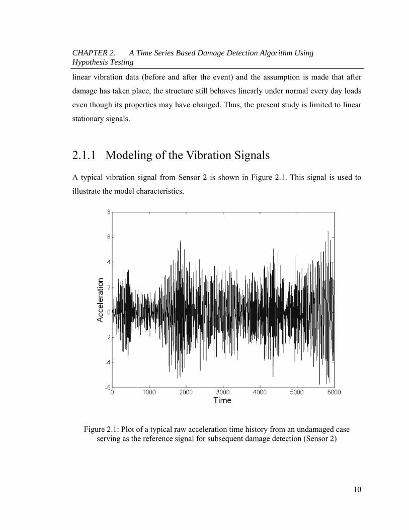
A typical vibration signal from Sensor 2 is shown in Figure 2.1. This signal is used to
illustrate the model characteristics.
Figure 2.1: Plot of a typical raw acceleration time history from an undamaged case serving as the reference signal for subsequent damage detection (Sensor 2)

CHAPTER 2. A Time Series Based Damage Detection Algorithm Using Hypothesis Testing
11
Before fitting a time series model to the sensor data, it is important to perform
standardization (or normalization) in order to compare acceleration time histories (at a
sensor location) that may have occurred due to different loading conditions (i.e., different
magnitudes and directions of loads) and/or different environmental conditions. After
normalization the features extracted from the signals from undamaged cases would have
similar statistical characteristics and can be compared.
Let xi(t) (i = 1,…,N) be the acceleration signal from sensor i, where N is the number of
sensors. This sensor signal is then partitioned into different streams xij(t) (i = 1,…,N and j
= 1,…,M), where i denotes the sensor number, j denotes the jth stream of data from the
sensor i and M is the number of streams. Then, the normalized signal txij~ is obtained as
follows:
ij
ijijij
txtx
~ (2.1)
where, ij and ij are the mean and standard deviation of the jth stream of sensor i
respectively. For notational convenience, xij(t) will be used instead of txij~ in the
subsequent development.
The next step is to check for trends and stationarity in the data (Brockwell and Davis,
2002), which can be achieved by observing the autocorrelation function (ACF). Figure
2.2 shows that the autocorrelation function of the normalized data has a cyclical trend
that will need to be removed. For detrending the data, three methods are used: (i)
harmonic regression, (ii) simple average window and (iii) moving average window
(Brockwell and Davis, 2002). It is found that harmonic regression could not remove the
trends and thus a combination of the simple average window and the moving average
window is used. The window sizes are chosen so that the residuals obtained from this
process are stationary. A review of the autocorrelation plot or the Ljung-Box statistic
provides further test that this condition is met. A more detailed explanation of the Ljung
Box statistic is provided later.

CHAPTER 2. A Time Series Based Damage Detection Algorithm Using Hypothesis Testing
12
Once the initial data pre-processing is complete, the optimal ARMA model order and its
coefficients are estimated (Brockwell and Davis, 2002). The ARMA model is given by:
p
k
q
kijijkijkij tktktxtx
1 1
(2.2)
where, xij(t) is the normalized acceleration signal, k and k are the kth AR and MA
coefficient respectively; p and q are the model orders of the AR and MA processes
respectively and ij(t) is the residual term. Also, note that the AR model is an ARMA
model when the order of the MA terms is zero. The AR model is given by
p
kijijkij tktxtx
1
(2.3)
Figure 2.2: Autocorrelation function of the normalized signal

CHAPTER 2. A Time Series Based Damage Detection Algorithm Using Hypothesis Testing
13
The Burg and Innovations algorithms are used for estimating the coefficients of the AR
and ARMA processes, respectively (Brockwell and Davis, 2002). The optimal model
order is obtained using the Akaike Information Criteria (AIC) (Brockwell and Davis,
2002). The AIC consists of two terms, one of which is a log-likelihood function and the
other term, which penalizes the number of terms in the time series model. AIC is defined
as:
12log2 qpMLAIC (2.4)
where, ML is the value of the maximum likelihood obtained.
Figure 2.3a shows the variation of the AIC values with the AR model order for different
MA orders. It is observed that, for as the MA model orders vary from q = 0 to 3, there is
very little difference in the AIC values of the AR and ARMA models at each model order
p. Since the AR process is the simpler model, it is chosen as the optimal time series
model that captures the characteristics of the signal. From the variation of the values of
AIC, it is observed that an AR model order of 5-8 is appropriate for the analysis. In
addition, a cross validation analysis is carried out to check the accuracy of the results.
This is performed as follows: for a particular data stream, the data set is split in two, one
is used for the analysis and the other is used for forecasting. In the analysis part, the
coefficients of the AR / ARMA model are calculated. Using these coefficients, the values
of the acceleration data are predicted. The residual error between the predicted values and
actual values are obtained. The root mean square (rms) value of the residual error is
plotted in Figure 2.3b. As expected, the rms value of the error decreases with the model
order and it is seen that model orders of 5-8 are appropriate for further analysis.
In order to obtain the AR coefficients, the Burg Algorithm is applied. Then the residuals
are tested to determine if they are normal, independent and identically distributed (i.i.d).
These tests are illustrated in Figure 2.4.

CHAPTER 2. A Time Series Based Damage Detection Algorithm Using Hypothesis Testing
14
(a)
(b)
Figure 2.3: Determination of Optimal AR model order (a) Variation of AIC with AR model order for MA orders varying from 0 to 3 and (b) Variation of cross validation error
with AR model order
Figure 2.4a shows the normal probability plot of the residuals. The straight line variation
indicates a normal distribution of the data, which is violated only at the tails. Figure 2.4b
CHAPTER 2. A Time Series Based Damage Detection Algorithm Using Hypothesis Testing
15
shows the variation of the residuals with time. It is seen that there is no trend, therefore,
indicating homoskedasticity. Figure 2.4c shows the autocorrelation function of the
residuals, from which it is observed that the values of the ACF at lags greater than one
are not statistically significant. The Ljung-Box statistic is also used to test the i.i.d
assumption of the AR residuals. The Ljung-Box statistic is defined as follows:
h
jLB jn
jnnQ
1
2
2 (2.5)
where n is the sample size, (j) is the autocorrelation function at lag j, and h is the
number of lags being tested. The null hypothesis of randomness is rejected if QLB>21-,h,
where is the level of significance of the hypothesis test and 21-,h is the (1-)th
percentile of the 2 distribution with h degrees of freedom. For this particular dataset, the
null hypothesis is not rejected. Thus, the assumptions made on the residuals are satisfied.
The total duration of the record xi(t) is 480 seconds. The record is divided into 80
segments, denoted by xij(t), j=1,2…80, each having 6 seconds duration sampled at 1000
Hz resulting in 6000 data points per segment. The AR coefficients are computed for each
six second segment of the acceleration data and the first three AR coefficients are used
for the calculation of the DSF. To determine the sensitivity of the coefficients to the
number of data points in the signal, analyses were performed in the range of 1000 to 6000
points in increments of 1000. The AR coefficients were found to reach stable values at
about 3000 points; however, 6000 points were used in the analysis presented in this
study. The stability of the first AR coefficients with the number of data points is
presented in Table 2.1. Both the mean and standard deviation of the coefficients are listed
in this table.

CHAPTER 2. A Time Series Based Damage Detection Algorithm Using Hypothesis Testing
16
(a) (b)
(c)
Figure 2.4: Verification of the i.i.d characteristics and normality of residuals: (a) Variation of residuals with time. (b) Normal probability plot of the residuals. (c)
Variation of the autocorrelation function of the residuals with lag.

CHAPTER 2. A Time Series Based Damage Detection Algorithm Using Hypothesis Testing
17
Table 2.1: Sensitivity of AR coefficients to the number of data points
Value of AR Coefficients
Number of Data Points 1000 2000 3000 4000 5000 6000
Mean of 1
(Std. Deviation of 1) 1.0441
(0.1947)1.0587
(0.1369)1.0566
(0.1088)1.0453
(0.0981) 1.0359
(0.0831) 1.0301
(0.0788)Mean of 2
(Std. Deviation of 2) 1.0359
(0.1966)1.0502
(0.1373)1.0517
(0.1002)1.0459
(0.0840) 1.0403
(0.0710) 1.0358
(0.0582)Mean of 3
(Std. Deviation of 3) 1.2204
(0.1366)1.2644
(0.0861)1.2772
(0.0608)1.2762
(0.0451) 1.2761
(0.0360) 1.2712
(0.0338)
2.1.2 Development of Damage Sensitive Feature (DSF)
In this section, the autoregressive coefficients are used to develop features that
discriminate between damaged and non-damaged states of a structure. Several damage
sensitive features (DSF) were investigated. Of the various DSFs considered, those
depending on the first three AR coefficients appeared to be most promising because these
coefficients are statistically the most significant among all the coefficients of the model.
After testing several different combinations with the first three coefficients (as is shown
in Section 2.1.3), it was found that the first AR coefficient normalized by the square root
of the sum of the squares of the first three AR coefficients provides the most robust
damage sensitive feature. Thus, the proposed damage sensitive feature (DSF) is defined
as follows:
23
22
21
1
DSF (2.6)
where 1, 2 and 3 are the first three AR coefficients. Variations of the DSF with the
record number for different damage patterns are illustrated in Figure 2.5. From these
figures it can be seen that for all damage patterns there is a significant difference in the

CHAPTER 2. A Time Series Based Damage Detection Algorithm Using Hypothesis Testing
18
mean levels of the DSF’s of the damaged and the undamaged states. Thus, to test
statistical difference between the means of two groups of data, the standard t-test is used
(Rice, 1999).
2.1.3 Correlation of the AR Coefficients to the Structural
System
The AR coefficients generally contain information about the modal natural frequencies
and the damping ratios (Maia and Silva, 1998; Lynch, 2004). The ARMA model in the
context of the linear input vibration (assuming to be white noise) may then be treated as
an autoregressive model with exogenous input (ARX) time series, where the input is a
white noise excitation. This model can be examined in the complex z-domain by applying
the time-shifting property of the z-transform (Oppenheim and Schafer, 1986). The z-
transform of a function f(t), denoted by F(z), is defined as follows (Oppenheim and
Schafer, 1986):
k
kzkfzF (2.7)
For a signal shifted by a time units, f(t-a), the z-transform of f(t-a) is given as follows:
zF z atfZ -a (2.8)
This is known as the time shifting property of the z-transform.
Applying the z-transform to both sides of Equation (2.2) and ignoring the effect of the
error term, we get
p
k
q
kij
kkij
kkij zzzXzzX
1 1
(2.9)

CHAPTER 2. A Time Series Based Damage Detection Algorithm Using Hypothesis Testing
19
where, Xij(z) and ij(z) are the z-transforms of the xij(t) and ij(t) respectively. Then, the
transfer function H(z) is derived as
p
p
ij
ij
zzz
zzz
z
zXzH
...1
...2
21
1
22
11
(2.10)
The denominator of the transfer function [H(z)] is a polynomial equation of order p
known as the characteristic equation. The roots of the characteristic equation, known as
the poles of the system, are expressed as follows:
0...22
11
pppp zzz (2.11)
The poles, zpole, of the characteristic equation are a good indicator of the modal natural
frequencies and the damping ratios given by (Maia and Silva, 1998):
tjt
pole
nn
ez21
(2.12)
where, and n are the damping ratio and natural frequency of the particular mode and
t is the sampling time of the signal. Equation (2.12) may be rewritten as jpole rez ,
where the amplitude r and phase angle are expressed as
;tner (2.13)
tn 21 (2.14)
Using simple theory of polynomial roots, it can be shown that
1, i
ipolez (2.15)
2,
,, ji
jpoleipole zz (2.16)
3,,,
,, kpolekji
jpoleipole zzz (2.17)

CHAPTER 2. A Time Series Based Damage Detection Algorithm Using Hypothesis Testing
20
(a)
(b)
(c)
(d)
(e)
(f)
Figure 2.5: Variation of DSF with record number for different damage patterns for Sensor 2: (a) Damage Pattern 1, (b) Damage Pattern 2, (c) Damage Pattern 3, (d) Damage Pattern
4, (e) Damage Pattern 5 and (f) Damage Pattern 6.

CHAPTER 2. A Time Series Based Damage Detection Algorithm Using Hypothesis Testing
21
Without loss of generality, p is assumed to be even and all the poles to be imaginary.
Thus, Equation (2.15) can be rewritten as follows:
2
11,1 cos2
p
iii
p
iipole rz (2.18)
Differentiating with respect to a parameter i, say an element of the stiffness matrix, we
get
2
1
11
p
j i
j
ji
k
k (2.19)
where, ki is the ith modal stiffness. Differentiating with respect to ki and assuming that the
damping ratio is a constant in each mode, we get the following
iiii
ii
i
i
iiii
i
i
i
km
tr
kr
k
r
k
sin1cos
sin2cos2
2
1
(2.20)
where n,i is the ith natural frequency, ti
inier , and tinii ,21 . Taking the
absolute value of the sensitivity ik
1 and since the sampling interval is generally small
and in the range of 0.005-0.02 seconds, we get
iiii
i
i km
t
km
tr
k
1 (2.21)
To obtain an approximation for i
ik
, the sensitivities of eigenvalues and eigenvectors
are used. These are discussed below.

CHAPTER 2. A Time Series Based Damage Detection Algorithm Using Hypothesis Testing
22
The eigenvalues and eigenvectors of a N degree of freedom system is obtained by solving
the following eigenvalue problem
Nrrrr ,..,1 allfor 02 MvKv (2.22)
where vr is the rth eigenvector corresponding to the eigenvalue ωr
2, and K and M are the
mass and stiffness matrices respectively. Differentiating Equation (2.22) with respect to
parameter θi (say an element of the stiffness matrix), to get
i
rrr
i
rr
i
rr
i
v
MvMv
KvK 22 (2.23)
Pre-multiplying with the transpose of vs and simplifying to get
i
rTsrsr
i
Tsr
Ts
i
rr
v
MvvK
vvMv 222 (2.24)
Using the orthogonality property and r = s, we get
ri
Tr
rTrri
r vK
vvMv
2
1 (2.25)
It is also shown in (Fox and Kapoor, 1968; Nelson, 1976) that the eigenvector sensitivity
is a linear combination of the eigenvectors, i.e.,
N
jr
irj
i
r
1
vv
(2.26)
where irj can be derived as (Nelson, 1976)
jr
jr
ri
Tj
jr
ri
ri
Tj
irj
for 2
1
for 22
2
vM
v
vMK
v
(2.27)
Since θi is one of the coefficients of the stiffness matrix, we get

CHAPTER 2. A Time Series Based Damage Detection Algorithm Using Hypothesis Testing
23
jr
jrjr
ri
Tj
irj
for 0
for 22
vK
v
(2.28)
To obtain the derivative of the rth modal stiffness with respect to θi, i
rk
, differentiate
the equation kr = ωr2 mr, we get
ri
Tr
ri
rrr
i
r mk
Mvv
222 (2.29)
Using Equations (2.25) and (2.28), Equation (2.29) can be expressed as
ri
Tr
N
rjj
jjr
ri
Tj
rri
Tr
i
rkMv
vv
vK
v
vK
v
1
2222 (2.30)
This can be further simplified by using the orthogonality principle
ri
Tr
i
rkv
Kv
(2.31)
Since vr is normalized, it can be concluded that
1
i
rk (2.32)
Thus we can conclude that
2
1
1
p
i iii km
t (2.33)

CHAPTER 2. A Time Series Based Damage Detection Algorithm Using Hypothesis Testing
24
Similar equations can be derived for i
2 and i
3 . Thus, it can be concluded that as the
stiffness decreases due to damage, the response of the structure will change resulting in
changes of the AR coefficients. Consequently, the damage sensitive feature based on the
AR coefficients can capture this change in measurements from an undamaged to
damaged structural state.
2.2 Damage Detection Algorithm Synthesis
The damage detection algorithm is summarized in the following steps:
Obtain signals from an undamaged structure, from sensor i, denoted by xi(t) (i = 1,…,
N), where N is the number of sensors. Segment the signal xi into chunks, xij(t) (j =
1,…, M), where M is the number of chunks. Populate a database with these baseline
signals.
Standardize the signal xij(t) to remove all trends and environmental conditions to
obtain txij~ .
Obtain signals from a potentially damaged structure for the same sensor, denoted by
zi(t), (i = 1,…, N). As in the previous steps, zi(t) is segmented into zij(t) (j = 1,…, M)
and is standardize to obtain tzij~ .
Fit an AR model to the signals txij~ and tzij
~ for all i and j.
For each sensor i, define and compute the statistics of damage sensitive feature, DSF,
for each chunk in the pre- and post-event signals. Compute the mean and pooled
variance of the DSF for the pre- and post-event signals.

CHAPTER 2. A Time Series Based Damage Detection Algorithm Using Hypothesis Testing
25
Determine the statistical significance in the differences of mean values of the pre- and
post- event data using the t-test to report the damage decision at sensor i. Report the
p-value and the confidence intervals of the differences in the mean of the DSF for the
pre- and post-event signals.
Report the damage decision.
The advantage of the damage detection algorithm presented in this section is that it
depends on signals obtained at a specified location on of a structure. With current smart
sensing capabilities that provide computational power at the sensor location, the
algorithm can be embedded and executed at the data collection site. Because of its
simplicity, the algorithm also can be executed rapidly and efficiently providing critical
information in a timely manner.
2.3 Application Results
In order to test the validity of the algorithm, vibration signals obtained from the
numerical simulation study of the ASCE Benchmark Structure are used. The structure is a
four story, two-bay by two-bay steel braced frame, illustrated in Figure 2.6 (Johnson et
al., 2004). There are 16 sensors (measuring acceleration) in the building, and their
placement and direction of the measured acceleration are shown in Figure 2.7 (Johnson et
al., 2004). Damage is simulated by removing braces in various combinations, resulting in
a loss of stiffness. Damage patterns include
Damage pattern 1: Removal of all braces on the first floor (near sensors 1-4)
Damage pattern 2: Removal of all braces on the first and third floors (near sensors 1-4
and 9-12)
Damage pattern 3: Removal of one brace on the first floor (near sensor 2)

CHAPTER 2. A Time Series Based Damage Detection Algorithm Using Hypothesis Testing
26
Damage pattern 4: Removal of one brace on the first (near sensor 2) and third floors
(near sensor 9)
Damage pattern 5: Damage pattern 4 + loosening of bolts near sensor 3
Damage pattern 6: Partial reduction of stiffness of one brace on the first floor (near
sensor 2)
Damage patterns 1 and 2 are major damage patterns, whereas damage patterns 4 and 5 are
moderate damage patterns; and damage patterns 3 and 6 are minor damage patterns.
Figure 2.6: ASCE Benchmark Structure (Johnson et al., 2004)
In the numerical simulation study of the benchmark structure, two finite element models
were used to generate the simulated response data: a 12 degree of freedom (DOF) shear-
building model that constrains all motion except two horizontal translations and one
rotation per floor and the second is a 120-DOF model that requires that floor nodes have

CHAPTER 2. A Time Series Based Damage Detection Algorithm Using Hypothesis Testing
27
the same horizontal translation and in-plane rotation. The columns and floor beams are
modeled as Euler–Bernoulli beams and the braces have no flexural stiffness. There are
two loading conditions on the ASCE Benchmark. The first excitation is a series of
independent filtered Gaussian white noise loads generated using a sixth - order low-pass
Butterworth filter with a 100 Hz cutoff and applied at each story of the structure. This
load is intended to model wind or ambient vibration forces. The second loading is a
random excitation generated by a shaker on the roof-top of the center column.
x y
Face 1
Face 2
Face 3
Face 4
Figure 2.7: Placement of sensors and direction of acceleration in the ASCE Benchmark Structure (http:// wusceel.cive.wustl.edu/ asce.shm/ benchmarks.htm)
CHAPTER 2. A Time Series Based Damage Detection Algorithm Using Hypothesis Testing
28
2.3.1 Damage Detection
Figure 2.5 shows the results from the application of the proposed damage algorithm to
the numerically simulated datasets of the ASCE Benchmark structure. From Figure 2.5
(a) – (f), it can be observed that there is a significant difference between the mean values
of the DSF’s obtained from the damaged and undamaged cases. To test the significance
of the difference in means of the DSF’s, a t-test is used (Rice, 1999).
If DSF, damaged and DSF, undamaged are defined as the mean values of the DSF’s obtained
from the damaged and undamaged case, respectively, then a hypothesis test may be set up
as follows to determine if their differences are significant:
damagedDSFundamagedDSF
damagedDSFundamagedDSF
H
H
,,1
,,0
:
:
(2.34)
where H0 and H1 are the null and alternate hypothesis respectively. H0 represents the
undamaged condition and H1 represents the damaged condition. The significance level of
the test is set at 0.05. The hypothesis used in Equation (2.34) is called a two-sided
alternative. For testing the above hypothesis, the t-statistic is used (Rice, 1999). The t-
statistic is defined as follows:
mns
t damagedDSFundamagedDSF
11
,,
(2.35)
where, m and n are the number of samples obtained from DSF of the damaged and
undamaged signals respectively; and s is the pooled sample variance, given as
2
11 2,
2,2
nm
SmSns damagedDSFundamagedDSF
(2.36)
where S2
() is the sample variance of (). For H1, the rejection region is defined as
CHAPTER 2. A Time Series Based Damage Detection Algorithm Using Hypothesis Testing
29
22mntt (2.37)
where tn+m-2(/2) is the value of the t-distribution with n+m-2 degrees of freedom
obtained at /2. Also, the confidence interval of the difference between DSF, undamaged -
DSF, damaged is given as:
mn
stCI nmdamagedDSFundamagedDSF
11
2ˆˆ 2,,
(2.38)
Tables 2.2 -2.6 show the results of the damage decision results for damage patterns 1-6
for the numerical simulation study. The p-value, the point estimate and confidence
intervals of the differences in the means of the undamaged and damaged signals are
presented. The p-value is the probability that the DSF does not predict damage, given in
fact that there is damage in the structure. The p-value is a preliminary indicator of
damage. However, the difference in the means, DSF, undamaged - DSF, damaged, also needs to
be high compared to other values obtained at other sensor locations. These are indicated
by its point estimate and the confidence intervals.

CHAPTER 2. A Time Series Based Damage Detection Algorithm Using Hypothesis Testing
30
Table 2.2: Results of damage decision for damage pattern 1
Sensor No.
Damage Decision
p-value Point Estimate of DSF, undamaged - DSF, damaged
CI of DSF, undamaged - DSF, damaged
1 H1 0.0 -0.2656 [-0.2956, -0.2357] 2 H1 0.0 0.3628 [0.3131, 0.4126] 3 H1 1.376710-13 -0.1290 [-0.1577, -0.1003] 4 H1 0.0 0.4495 [0.4082, 0.4909] 5 H1 5.3951e-007 0.0795 [0.0506, 0.1085] 6 H1 0.0 0.5623 [0.5179, 0.6068] 7 H1 0.0097 0.0391 [0.0098, 0.0685] 8 H1 0.0 0.4816 [0.4318, 0.5314] 9 H1 0.0 -0.1769 [-0.2057, -0.1481]
10 H1 0.0 0.2139 [0.1768, 0.2510] 11 H1 0.0 -0.1708 [-0.2011, -0.1405] 12 H1 2.6302e-011 0.1325 [0.0985, 0.1664] 13 H1 8.8818e-016 -0.1539 [-0.1843, -0.1235] 14 H1 0.0389 0.0395 [0.0021, 0.0768] 15 H1 0.0 -0.2320 [-0.2660, -0.1980] 16 H0 0.8026 0.0039 [-0.0267, 0.0344]
Table 2.3: Results of damage decision for damage pattern 2
Sensor No.
Damage Decision
p-value Point Estimate of DSF, undamaged - DSF, damaged
CI of DSF, undamaged - DSF, damaged
1 H1 0.0 0.3999 [0.3457, 0.4540] 2 H1 0.0 0.9858 [0.9357, 1.0359] 3 H1 0.0 0.2592 [0.2080, 0.3104] 4 H1 0.0 0.8598 [0.8125, 0.9071] 5 H1 0.0 0.2958 [0.2503, 0.3414] 6 H1 0.0 0.4600 [0.4054, 0.5147] 7 H1 0.0 0.2736 [0.2295, 0.3176] 8 H1 0.0 0.5553 [0.5006, 0.6100] 9 H1 0.0 0.4339 [0.4071, 0.4607]
10 H1 0.0 0.2412 [0.2046, 0.2777] 11 H1 0.0 0.3826 [0.3544, 0.4108] 12 H1 0.0 0.2721 [0.2368, 0.3075] 13 H1 0.0 0.2698 [0.2346, 0.3049] 14 H1 0.0 0.3488 [0.2321, 0.4656] 15 H1 0.0 0.2689 [0.2321, 0.3058] 16 H1 0.0 0.2793 [0.2280, 0.3305]

CHAPTER 2. A Time Series Based Damage Detection Algorithm Using Hypothesis Testing
31
Table 2.4: Results of damage decision for damage pattern 3
Sensor No.
Damage Decision
p-value Point Estimate of DSF, undamaged - DSF, damaged
CI of DSF, undamaged - DSF, damaged
1 H0 0.2732 0.0212 [-0.0533, 0.0152] 2 H1 1.174010-10 0.1455 [0.1065, 0.1845] 3 H0 0.2886 0.0182 [-0.0156, 0.0520] 4 H1 8.989510-4 0.0669 [0.0283, 0.1055] 5 H0 0.2478 -0.0163 [-0.0441, 0.0116] 6 H1 0.0 0.1784 [0.1477, 0.2091] 7 H1 0.0305 -0.0298 [-0.0567, -0.0029] 8 H1 0.0337 0.0356 [0.0028, 0.0685] 9 H1 0.0 -0.1817 [-0.2129, -0.1505]
10 H1 1.801310-7 0.0814 [0.0531, 0.1097] 11 H1 6.064710-9 -0.1122 [-0.1464, -0.0780] 12 H1 0.0115 0.0406 [0.0094, 0.0719] 13 H1 1.444810-12 -0.1595 [-0.1972, -0.1218] 14 H1 7.755310-4 -0.0528 [-0.0829, -0.0228] 15 H1 4.624610-8 -0.1242 [-0.1651, -0.0834] 16 H1 1.401810-8 0.0971 [0.0666, 0.1277]
Table 2.5: Results of damage decision for damage pattern 4 and 5
Sensor No.
Damage Decision
p-value Point Estimate of DSF, undamaged - DSF, damaged
CI of DSF, undamaged - DSF, damaged
1 H1 0.0031 0.0475 [0.0166, 0.0785] 2 H1 1.032410-11 0.1528 [0.1147, 0.1909] 3 H1 4.440910-16 0.1567 [0.1262, 0.1871] 4 H1 6.390510-6 0.0902 [0.0531, 0.1273] 5 H1 6.149410-5 0.0556 [0.0295, 0.0818] 6 H1 1.974010-13 0.1360 [0.1055, 0.1666] 7 H1 2.961410-8 0.0855 [0.0578, 0.1131] 8 H0 0.6574 0.0074 [-0.0259, 0.0407] 9 H1 6.685610-7 0.0865 [0.0547, 0.1183]
10 H1 2.793710-9 0.0949 [0.0667, 0.1231] 11 H1 1.508210-10 0.1329 [0.0970, 0.1688] 12 H1 0.0023 0.0487 [0.0179, 0.0794] 13 H1 6.924210-7 -0.0841 [-0.1151, -0.0531] 14 H0 0.2571 -0.0170 [0.0467, 0.0127] 15 H1 8.215510-4 -0.0628 [-0.0987, -0.0269] 16 H1 2.723810-9 0.1002 [0.0705, 0.1299]

CHAPTER 2. A Time Series Based Damage Detection Algorithm Using Hypothesis Testing
32
Table 2.6: Results of damage decision for damage pattern 6
Sensor No.
Damage Decision
p-value Point Estimate of DSF, undamaged - DSF,
damaged
CI of DSF, undamaged - DSF, damaged
1 H0 0.6826 -0.0048 [-0.0280, 0.0184] 2 H1 2.853310-8 0.0942 [0.0674, 0.1211] 3 H0 0.1799 0.0221 [-0.0104, 0.0545] 4 H1 1.981010-5 0.0772 [0.0434, 0.1110] 5 H0 0.8578 -0.0024 [-0.0294, 0.0245] 6 H1 8.368810-9 0.0949 [0.0656, 0.1241] 7 H0 0.7112 -0.0051 [-0.0322, 0.0221] 8 H1 3.427410-4 0.0533 [0.0250, 0.0816] 9 H1 0.0295 0.0157 [0.0016, 0.0298] 10 H1 0.0010 0.0501 [0.0208, 0.0794] 11 H0 0.3203 -0.0166 [-0.0495, 0.0164] 12 H1 0.0163 0.0376 [0.0071, 0.0680] 13 H0 0.0967 -0.0291 [-0.0636, 0.0054] 14 H1 0.0085 0.0382 [0.0100, 0.0663] 15 H0 0.2768 -0.0211 [-0.0595, 0.0173] 16 H1 1.720510-9 0.0940 [0.0666, 0.1214]
The conclusions drawn from the damage detection results are as follows:
In the case of major damage patterns 1 and 2, it is observed that the difference in the
means of the damaged and undamaged signals is statistically significant. However, in
the case of damage pattern 1, the t-test indicates that there is no damage at sensor 16.
For sensors 5, 7 and 14, it is observed that the difference in the means is small as
compared to other sensors. For damage pattern 2, all sensors show a statistical
significant difference in the means, thus indicating damage.
Bolt loosening (near sensor 3) was not detected in damage pattern 5. The maximum
difference in the means is obtained at sensors 2, 3 and 6. Again note that sensors 8
and 14 do not indicate damage, whereas sensors 1 and 12 have a very minor
difference in the means. Here again, damage has been consistently detected for
moderate damage patterns 4 and 5.
CHAPTER 2. A Time Series Based Damage Detection Algorithm Using Hypothesis Testing
33
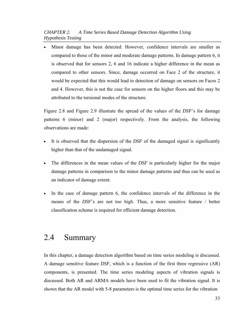
Minor damage has been detected. However, confidence intervals are smaller as
compared to those of the minor and moderate damage patterns. In damage pattern 6, it
is observed that for sensors 2, 6 and 16 indicate a higher difference in the mean as
compared to other sensors. Since, damage occurred on Face 2 of the structure, it
would be expected that this would lead to detection of damage on sensors on Faces 2
and 4. However, this is not the case for sensors on the higher floors and this may be
attributed to the torsional modes of the structure.
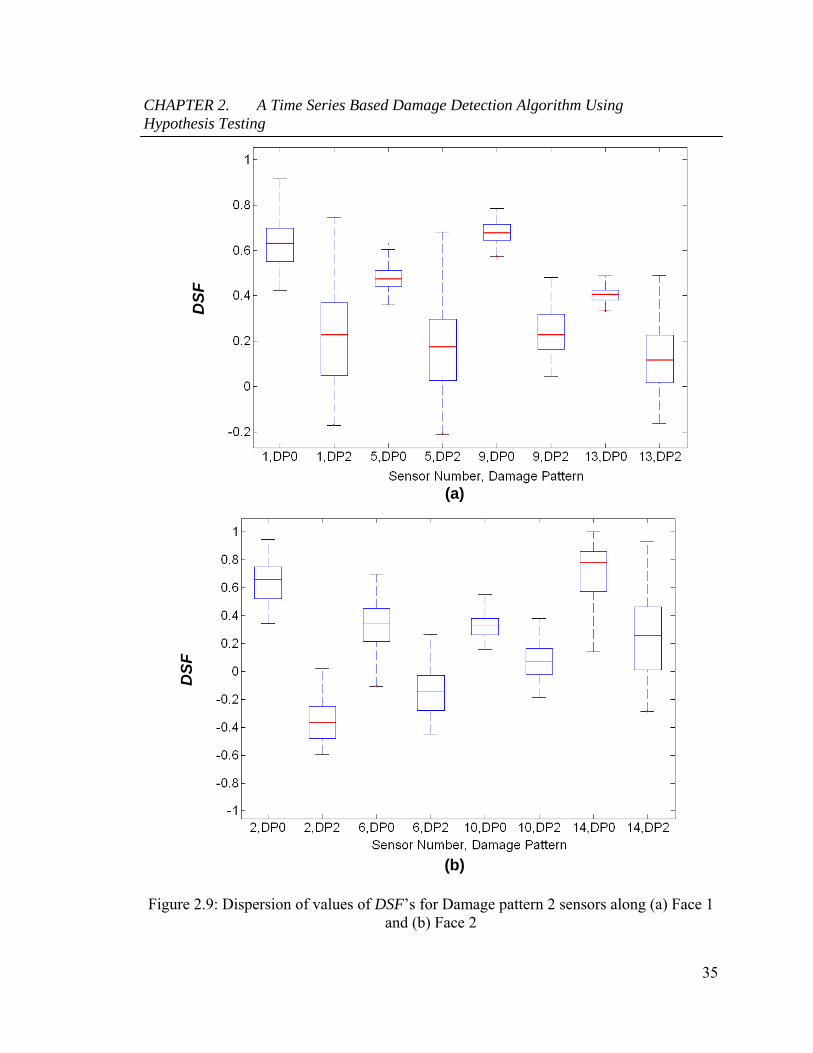
Figure 2.8 and Figure 2.9 illustrate the spread of the values of the DSF’s for damage
patterns 6 (minor) and 2 (major) respectively. From the analysis, the following
observations are made:
It is observed that the dispersion of the DSF of the damaged signal is significantly
higher than that of the undamaged signal.
The differences in the mean values of the DSF is particularly higher for the major
damage patterns in comparison to the minor damage patterns and thus can be used as
an indicator of damage extent.
In the case of damage pattern 6, the confidence intervals of the difference in the
means of the DSF’s are not too high. Thus, a more sensitive feature / better
classification scheme is required for efficient damage detection.
2.4 Summary
In this chapter, a damage detection algorithm based on time series modeling is discussed.
A damage sensitive feature DSF, which is a function of the first three regressive (AR)
components, is presented. The time series modeling aspects of vibration signals is
discussed. Both AR and ARMA models have been used to fit the vibration signal. It is
shown that the AR model with 5-8 parameters is the optimal time series for the vibration

CHAPTER 2. A Time Series Based Damage Detection Algorithm Using Hypothesis Testing
34
(a)
(b)
DS
F
DS
F
Figure 2.8: Dispersion of Values of DSF’s for Damage Pattern 6 sensors along (a) Face 1 and (b) Face 2
CHAPTER 2. A Time Series Based Damage Detection Algorithm Using Hypothesis Testing
35
(a)
(b)
DS
F
DS
F
DS
F
DS
F
Figure 2.9: Dispersion of values of DSF’s for Damage pattern 2 sensors along (a) Face 1 and (b) Face 2

CHAPTER 2. A Time Series Based Damage Detection Algorithm Using Hypothesis Testing
36
signals considered in the study. Subsequently, a closed form equation relating the AR
coefficients with the parameters of the physical system is derived.
Next, a hypothesis test involving the t-test is used to obtain a damage decision. The
damage detection methodology is tested on the analytical results of the ASCE Benchmark
Structure. The results of the application of this damage detection algorithm indicates that
the algorithm is able to detect the existence of all damage patterns in the ASCE
Benchmark simulation experiment where minor, moderate and severe damage
corresponds to removal of single brace in a storey, removal of a brace on two storeys and
removal of all braces in two storeys, respectively. These results are very encouraging, but
represent initial testing of the algorithm and further investigations will be needed to test
the validity of the damage detection method. More testing is needed to investigate various
scenarios and conditions that introduce other damage patterns, such as cracking at joints
or loosening of bolts. While it may be difficult to simulate such conditions numerically,
they can be reproduced in the laboratory. Thus, additional testing will be performed as
such data become available. Ultimately, these algorithms will need to be tested with field
data.
The advantage of the statistical signal processing approach combined with the pattern
classification framework is that it does not require any elaborate finite element modeling.
Such an approach is particularly suited for wireless sensor analysis, which is able to
process data at the sensor unit location through embedded algorithms. Such data can then
be transmitted to a global master for additional damage analysis using system
identification methods.
37
Chapter 3
A Time Series Based Structural Damage Detection Algorithm Using Gaussian Mixture Modeling
In Chapter 2, it was shown that the damage sensitive feature (DSF) was able to detect
minor damage for the ASCE Benchmark Structure. However, it was also observed that
the confidence intervals for minor damage patterns were relatively smaller in comparison
to major damage patterns. Thus, a more robust classification scheme is needed to identify
minor damage patterns. To this end, a time series based detection algorithm utilizing the
Gaussian Mixture Models (GMM’s) is presented in Chapter 3.
Two critical aspects of damage diagnosis, detection and extent, are investigated. As in the
previous chapter, the vibration signals obtained from the structure are modeled as auto-
regressive (AR) processes. The feature vector used consists of the first three
autoregressive coefficients obtained from the modeling of the vibration signals. It is
observed that there is a migration of the extracted AR coefficients with increasing levels
of damage. To detect these changes in the AR coefficients, a clustering scheme called the
Gaussian Mixture Model (GMM) is used. Damage is detected if there is more than one
CHAPTER 3. A Time Series Based Structural Damage Detection Algorithm using Gaussian Mixture Modeling
38
cluster‡ in a particular dataset. This is achieved using the gap statistic, which determines
the optimal number of mixtures in that dataset. The Mahalanobis distance between the
mixture in question and the baseline (undamaged) mixture is investigated as a candidate
for quantifying damage extent. Application cases from the ASCE Benchmark Structure
simulated data are used to test the efficacy of the algorithm.
3.1 Overview of the Damage Diagnosis Algorithm
As discussed in Chapter 2, structural damage is detected using time series analysis of the
vibration signals measured from the pre-damaged and post-damaged states of the
structure. Figure 3.1 illustrates the effect of damage on the first three AR coefficients 1,
2 and 3. It is seen that the clouds of AR coefficients obtained by modeling vibration
signals before damage would migrate with the onset of damage. AR coefficients
corresponding to damage patterns 1 and 2 are plotted in this figure. Thus, the main
premise in the proposed algorithm is that there is a migration of clusters of the feature
vectors (AR coefficients) with damage.
The proposed algorithm is as follows:
1 Obtain signals (vibration and strain if available) from an undamaged structure,
from sensor i, denoted by xi(t) (i = 1,…,P), where P is the number of sensors.
Segment the signal xi(t) into chunks of finite duration xij(t) (j = 1,…,Q ), where Q
is the number of chunks. Populate the database with these baseline signals.
2 Model the chunks of time series data from each sensor as described in Chapter 2.
Extract the damage sensitive features from the signals that define them as feature
vectors. In this algorithm, the first three AR coefficients of the signals are used to
define the feature vectors. Denote the feature vectors as αi,baseline which is of
‡ In this dissertation, the words ‘cluster’ and ‘mixture’ and used interchangeably.

CHAPTER 3. A Time Series Based Structural Damage Detection Algorithm using Gaussian Mixture Modeling
39
dimension Q3. It should be noted that we use the signals obtained at each sensor
and local signal processing is performed at that sensor before and after damage.
Figure 3.1: Migration of feature vectors (defined by the first three AR coefficients) from an undamaged state to damage patterns 1 and 2 as defined by the ASCE Benchmark
Structure
3 Obtain signals from a potentially damaged structure for the same sensor, denoted
by zi(t), (i = 1,…, P). As in the previous steps, zi(t) is segmented into zij(t) (j =
1,…, Q). Again the first three AR coefficients are used to define feature vectors
for damage detection. Denote the new feature vectors as αi,new which is of
dimension Q3.
4 Define the feature vector Yi (i = 1,…, P), of dimension 2Q3, as follows
CHAPTER 3. A Time Series Based Structural Damage Detection Algorithm using Gaussian Mixture Modeling
40
newi
baselineii
,
,
α
αY (3.1)
5 Fix the number of clusters as k. For a fixed value of k, fit the feature vectors Yi,
defined in Equation (3.1), using a Gaussian mixture model (GMM) and obtain the
parameters of the GMM using the Expectation-Maximization (EM) algorithm.
Using the parameters of the GMM, calculate the gap statistic (Tibshirani et al.,
2001).
6 Use the gap statistic to determine the optimal number of clusters. If the number of
clusters is greater than one, then it is hypothesized that some degree of damage
has taken place. If, however, the clusters are very close based on the gap statistic,
then it is concluded that there is no damage. Such signals would be stored in the
baseline database.
7 If damage has occurred, using the covariance matrices obtained by using the EM
algorithm, calculate the Mahalanobis distance for the new mixture and the
baseline mixture.
8 Repeat steps 2-7 with the baseline data and the subsequent signals identifying
damage and quantifying damage according to steps 5, 6 and 7.
3.2 Modeling of Vibration Signals
In this subsection, the time series modeling of vibration signals is summarized. Details of
the various steps discussed below are available in Chapter 2. The main steps in the
modeling of vibration signals are listed below:
Standardize the vibration signal as described by Equation (2.1).
CHAPTER 3. A Time Series Based Structural Damage Detection Algorithm using Gaussian Mixture Modeling
41
Fit the autoregressive (AR) or the autoregressive moving average (ARMA)
models to the vibration signal.
Use the Akaike Information Criteria (AIC) to ascertain the optimal model orders
of the AR and MA coefficients. Figure 2.3(a) illustrates this step.
Check the assumption of the time series models fitted. These include the
homoskedasticity, the normality condition and the i.i.d assumptions of the
residuals. This is illustrated in Figure 2.4
With respect to the vibration signals obtained from the ASCE Benchmark Structure, it is
found that the AR model is the optimal time series with the AR model order being
between 5 and 8.
For the baseline and new signals, the total duration of each record is 480 seconds. Each
record is divided into 80 segments (i.e., Q = 80), denoted by xij(t), j=1,2…80, each having
6 seconds duration sampled at 1000 Hz resulting in 6000 data points per segment. The
AR coefficients are computed for each six second segment of the acceleration data and
the first three AR coefficients are used in a feature vector Yi, as given in Equation (3.1),
that has a size of 160 by 3.
3.3 Gaussian Mixture Modeling
Figure 3.1 illustrates the migration of the feature vectors at sensor 2 from its undamaged
state (2,undamaged) to damage patterns 1 (2,DP1) and 2 (2,DP2), resulting in the formation
of three unique clusters. It is recalled that damage pattern 1 represents braces removed
from the first floor and damage pattern 2 represents the removal of braces from the first
and third floor. Thus, an algorithm is required to ascertain the number of clusters in a
dataset. To this end, Gaussian mixture models are used. Gaussian mixture models
(GMM’s) are frequently used as clustering algorithms in pattern classification (Hastie et

CHAPTER 3. A Time Series Based Structural Damage Detection Algorithm using Gaussian Mixture Modeling
42
al., 2002). A Gaussian mixture model with M classes (or mixtures or clusters) has the
following form:
M
iiiiNf
1:1 ;Yy (3.2)
where, Y is the collection of N feature vectors (in this study N = 160), iii N ,~ is a
Gaussian vector with mean vector i and covariance matrix i and i is the non-negative
mixture weight for each class. The unknown parameters of the GMM = {i, i, i i =
1,2,…M} can be estimated using the maximum likelihood principle. The direct
maximization of the likelihood function is quite difficult and analytically intractable. For
this purpose, the expectation maximization (EM) algorithm is used. The derivation of the
EM algorithm is given in the Section 3.8. Define a random variable Ii (i = 1,..,N) whose
realization is an M dimensional indicator row vector, whose (i, j) component is 1 (i.e., Iij
= 1) if yi corresponds to the jth mixture. The EM algorithm in the context of the GMM is
as follows:
Step 1: Initialize the values of E(Iij) (i=1,…,N and j = 1,…,M), the mixture weights, the
means and covariance matrices of the classes of the GMM.
Step 2: The update equations are as follows:
N
kkj
N
kkkj
j
IE
IE
1
1
y (3.3)
N
kkj
N
k
Tjkjkkj
j
IE
IE
1
1
μyμyΣ (3.4)
N
IEN
kkj
j
1
(3.5)

CHAPTER 3. A Time Series Based Structural Damage Detection Algorithm using Gaussian Mixture Modeling
43
N
kkiki
jijiij
Ip
IpIE
1
;1|
;1|
y
y
(3.6)
Equations (3.3) - (3.5) constitute the maximization (M-step) and Equation (3.6)
constitutes the expectation (E-step) of the algorithm. It should be noted that
jijT
jijdiji Ip μyΣμyΣy 12
1
2/ 2
1exp
2
1;1| (3.7)
where d is the dimension of the feature vector xi.
Step 3 : Calculate the log-likelihood function given by Equation (3.17) at the tth and
(t+1)th time steps. The definition of the log-likelihood function is given in Section
3.8. At the end of each step, test for convergence using:
1
111
log
loglog
t
tt
L
LL (3.8)
where is assumed to be 0.001.
As discussed above, in Step 1 of the EM algorithm, some initial guesses of the
parameters has to be made. The k-means algorithm (Hastie et al., 2002) is frequently used
to obtain a first estimate of the means of the clusters and is described below:
Initialize the cluster means to M randomly chosen points (since there are M
clusters)
For each cluster mean, j, find the points in the dataset closest to j. Denote
these set of points as Mj and the number of points as nj.
Compute the new mean

CHAPTER 3. A Time Series Based Structural Damage Detection Algorithm using Gaussian Mixture Modeling
44
ji M
ij
j n y
yμ1
(3.9)
Iterate the above two steps until convergence is obtained.
Figure 3.2: Variation of log-likelihood with number of mixtures in the dataset
Figure 3.2 illustrates the variation of the log-likelihood with the number of mixtures. As
expected, as the number of mixtures increase, the log-likelihood increases.

CHAPTER 3. A Time Series Based Structural Damage Detection Algorithm using Gaussian Mixture Modeling
45
3.4 Damage Diagnosis using Gaussian Mixture
Models
As stated earlier, the main premise in the proposed algorithm is that there is a migration
of clouds of feature vectors obtained from sequential measurements as damage is
incurred to the structure. Damage is identified by determining that there is more than one
mixture in a particular dataset given by Equation (3.1). Damage extent is obtained using
the Mahalanobis distance between the centroid of the mixture distribution under question
with respect to the baseline mixture. The formulations required for estimating the number
of mixtures and the Mahalanobis distance between mixtures is described in the following
sections.
3.4.1 Damage Identification using the Gap Statistic
Figure 3.1 illustrates the migration of the feature vector clouds for the damage patterns
considered in the ASCE Benchmark structure. In order to discriminate between damage
and no damage in a given feature vector, the number of clusters or mixtures has to be
determined. The number of mixtures for a particular dataset is determined by using the
gap statistic (Tibshirani et al., 2001).
As before, we consider M clusters, C1, C2,…, CM. Let the number of observations in the
rth cluster be denoted by nr. Then the within cluster sum of squared distance of cluster r,
denoted as Dr is given as
22
,,
2
rrr Ci
irCji
jiCji
ijr ndD yyyy (3.10)
where dij is the sum of squared distance between the ith and jth observation. In most
situations, the Euclidean distance between observations is used. This is illustrated in
Figure 3.3. The dispersion measure is denoted as Wk and is defined by

CHAPTER 3. A Time Series Based Structural Damage Detection Algorithm using Gaussian Mixture Modeling
46
MkDn
Wk
rr
rk ,...1
2
1
1
(3.11)
Cluster r
Figure 3.3: Illustration of within cluster distance
The gap statistic is then given as follows (Tibshirani et al., 2001):
kknn WWEkGap loglog (3.12)
where En denotes the expectation with respect to some reference distribution. In this
study, the uniform distribution for the range of the observed values for that feature is
used, as proposed by Tibshirani et al., 2001. The estimate of k which maximizes the
Gapn(k) is the number of clusters in the dataset. Thus, for the computation of the gap
statistic, the following algorithm is used (Tibshirani et al., 2001):
Fix the number of clusters and then use the GMM’s to cluster the observed
data. For each of these cases, calculate Wk : k = 1,.., M.
Generate B reference datasets according to the uniform distribution and
calculate the dispersion measure Wkb for all b = 1,…,B, and k=1,…,M.
Compute the mean and the standard deviation as follows

CHAPTER 3. A Time Series Based Structural Damage Detection Algorithm using Gaussian Mixture Modeling
47
B
sdks
WB
ksd
WB
bckb
bkbc
11
log1
log1
2
1
2
(3.13)
Choose the number of clusters by using the rule given below
k
B
bkb
k
WWB
kGap
skGapkGapthatsuchksmallestk
loglog1
)1( ˆ
1
1
(3.14)
From the application of this algorithm, if the number of clusters k, is found to be greater
than one, it is hypothesized that the signals come from different states of the structure and
this change of state is most likely due to damage.
3.5 Damage Extent using the Mahalanobis Metric
The Mahalanobis distance is a metric frequently used in multivariate analysis to
determine the separation of two distributions (Mardia et al., 2003). The Mahalanobis
distance between two vectors a and b with a covariance matrix is defined as follows:
baΣbaΣba 1,, T (3.15)
In the present study, the Mahalanobis distance is used to define a measure of the damage
extent. More specifically, the damage metric DM used is defined as (undamaged, damaged;
undamaged) where undamaged is the covariance matrix of the undamaged dataset, undamaged
and damaged, are the means of the undamaged and damaged dataset respectively. These
values are obtained after modeling the feature vectors as a GMM. Mathematically, the
metric DM may be defined as:

CHAPTER 3. A Time Series Based Structural Damage Detection Algorithm using Gaussian Mixture Modeling
48
damagedundamagedundamaged
Tdamagedundamaged
undamageddamagedundamagedDM
μμΣμμ
Σμμ
1
;, (3.16)
The above formulation is valid for a two mixture dataset. However if the number of
mixtures is greater than two, the value of DM is chosen as the maximum of the values of
this measure computed between the undamaged mixture and the other mixtures.
3.6 Application
In order to test the validity of the algorithm, results from the numerical simulation of the
ASCE Benchmark Structure are used (Johnson et al., 2004). Details on the ASCE
Benchmark Structure are discussed in Chapter 2.
3.6.1 Damage Detection
Figures 3.4, 3.5 and 3.6 illustrate the migration of the clouds of feature vectors composed
of the first three AR coefficients with minor, moderate and major amounts of damage
respectively. Thus, the migration of the mixtures for each pair of data would give an
indication of damage. The gap statistic provides a means for tracking the number and
migration of mixtures. If two or more mixtures are identified through this statistic, then
there is high likelihood of damage occurrence.
Damage pattern 0 (DP0) represents the undamaged state and data from that feature vector
is taken as the baseline state. Feature vectors from progressively increasing damage are
compared to the baseline in order to identify the onset and increase in damage. The first
damage pattern considered for the comparison is damage pattern 6 because it is the
smallest damage imposed on the structure. Using the gap statistic, the number of mixtures
obtained is 2. This is illustrated in Figure 3.4a. Applying the algorithm, all damage
patterns 1-6 have been identified.

CHAPTER 3. A Time Series Based Structural Damage Detection Algorithm using Gaussian Mixture Modeling
49
(a)
(b)
Figure 3.4: Migration of the feature vectors with damage for minor patterns (a) Damage pattern 6 and (b) Damage Pattern 3

CHAPTER 3. A Time Series Based Structural Damage Detection Algorithm using Gaussian Mixture Modeling
50
(a)
(b)
Figure 3.5: Migration of the feature vectors with damage for moderate patterns (a) Damage pattern 4 and (b) Damage Pattern 5

CHAPTER 3. A Time Series Based Structural Damage Detection Algorithm using Gaussian Mixture Modeling
51
(a)
(b)
Figure 3.6: Migration of the feature vectors with damage for major patterns (a) Damage pattern 1 and (b) Damage Pattern 2

CHAPTER 3. A Time Series Based Structural Damage Detection Algorithm using Gaussian Mixture Modeling
52
Figure 3.7 illustrates the variation of the gap statistic with number of mixtures for a
damaged case. The feature vectors are plotted in Figure 3.7(a). Note that there is a clear
separation of clusters in this dataset, plotted in Figure 3.7(a). Figure 3.7(b) shows the
variation of the observed and expected value of log(Wk) with number of mixtures. The
variation of the gap statistic is plotted in Figure 3.7(c). It shows that the gap statistic
yields the highest value at the second mixture, thus showing that there are two mixtures,
indicating damage in the structure. Since the gap statistic gives an indication of the
dispersion of the dataset with respect to a uniformly distributed dataset, the optimal
number of mixtures is obtained at where the gap statistic is maximized. A similar
illustration of the gap statistic for an undamaged case is given in Figure 3.8, where there
is no clear separation of clusters in the dataset. The number of mixtures identified by the
gap statistic is one, indicating no damage. It is also noted that the value of the gap
statistic is very small implying that there is very little difference between the generated
uniform distribution and the feature vector.

CHAPTER 3. A Time Series Based Structural Damage Detection Algorithm using Gaussian Mixture Modeling
53
0.40.6
0.81
1.21.4
-1
0
1
20
0.5
1
1.5
1
2
3
Undamaged
Damaged
1 2 3 4 52.5
3
3.5
4
4.5
5
5.5
Number of Mixtures
Log-L
ikelih
ood
ObservedExpected
1 2 3 4 50
0.5
1
1.5
2
Number of Mixtures
Gap
(a)
(b)
(c)
Figure 3.7: Illustration of the gap statistic for a damaged case (a) Distribution of AR coefficients (b) Variation of the observed and expected value of log(Wk) with number of
mixtures (c) Variation of the gap statistic with number of mixtures

CHAPTER 3. A Time Series Based Structural Damage Detection Algorithm using Gaussian Mixture Modeling
54
0.7 0.8 0.9 1 1.1 1.2 1.3
0.81
1.21.4
1.61.1
1.2
1.3
1.4
1.5
1
2
3
Undamaged Set 1
Undamaged Set 2
1 2 3 4 51.5
2
2.5
3
Number of Mixtures
Log-
Like
lihoo
d
ObservedExpected
1 2 3 4 5-0.15
-0.1
-0.05
0
0.05
0.1
Number of Mixtures
Gap
(a)
(b)
(c)
Figure 3.8: Illustration of the gap statistic for an undamaged case (a) Distribution of AR coefficients (b) Variation of the observed and expected value of log(Wk) with number of
mixtures (b) Variation of the gap statistic with number of mixtures

CHAPTER 3. A Time Series Based Structural Damage Detection Algorithm using Gaussian Mixture Modeling
55
Table 3.1 shows the results of the EM algorithm, which yields the weights, means and
autocorrelation matrices of the feature vectors obtained from sensor 2 from its pre and
post damage states. It is observed that the weight associated with each mixture is between
0.4-0.5 for the presence of two mixtures and can be used as a simple rule of thumb for the
existence of more than one mixture.
Table 3.1: Results from the EM Algorithm for various damage patterns (DP)
DP Means Autocorrelation Matrices Weights
1
3282.0
1758.0
6709.0
2758.1
0407.1
0323.1
0000.18040.07866.0
8040.00000.18327.0
7866.08327.00000.1
0000.18730.07466.0
8730.00000.17130.0
7466.07130.00000.1
5000.0
5000.0
2
1347.0
6519.0
2057.0
2758.1
0407.1
0323.1
0000.11589.08849.0
1589.00000.14517.0
8849.04517.00000.1
0000.18730.07466.0
8730.00000.17130.0
7466.07130.00000.1
5000.0
5000.0
3
1317.1
8931.0
8861.0
2753.1
0403.1
0322.1
0000.16636.07072.0
6636.00000.14682.0
7072.04682.00000.1
0000.18700.07382.0
8700.00000.17123.0
7382.07123.00000.1
5032.0
4968.0
4
1145.1
8525.0
8795.0
2757.1
0406.1
0323.1
0000.15082.06312.0
5082.00000.13898.0
6312.03898.00000.1
0000.18731.07445.0
8731.00000.17124.0
7445.07124.00000.1
5005.0
4995.0
5
1145.1
8525.0
8795.0
2757.1
0406.1
0323.1
0000.15082.06312.0
5082.00000.13898.0
6312.03898.00000.1
0000.18731.07445.0
8731.00000.17124.0
7445.07124.00000.1
5005.0
4995.0
6
2419.1
9924.0
9369.0
2647.1
0494.1
0358.1
0000.17495.08832.0
7495.00000.16295.0
8832.06295.00000.1
0000.18611.08173.0
8611.00000.16760.0
8173.06760.00000.1
4642.0
5358.0

CHAPTER 3. A Time Series Based Structural Damage Detection Algorithm using Gaussian Mixture Modeling
56
3.6.2 Damage Extent
The damage extent is calculated using Equation (3.16) and the results of the DM
calculated for sensor 2 are shown in the semi-log plot in Figure 3.9. As can be observed
from this figure, the damage metric DM increases for damage patterns 6, 3, 4, 5, 1 and 2,
which corresponds to a progressive increase in damage. Also, DM varies from 2.95
(corresponding to damage pattern 6) to 4591.56 (corresponding to damage pattern 2).
Figure 3.9: Variation of the damage metric DM with damage pattern for sensor 2
The variation of the damage metric (DM) for various sensors and different damage
patterns is given in Table 3.2.

CHAPTER 3. A Time Series Based Structural Damage Detection Algorithm using Gaussian Mixture Modeling
57
Table 3.2: Variation of DM for various sensors and different damage patterns
DP1 DP2 DP3 DP4 DP5 DP6
1 431.38 1415.53 NA 50.90 50.90 NA 2 1374.21 4591.56 22.54 25.85 25.85 2.95 3 454.63 1673.77 NA 34.46 34.46 NA 4 1096.92 5993.50 32.33 48.73 48.73 2.78 5 295.61 826.69 NA 25.67 25.67 NA 6 1350.03 4306.10 21.79 24.04 24.04 2.64 7 265.79 703.07 NA 20.73 20.73 NA 8 858.93 3224.43 9.52 10.75 10.75 1.59 9 263.74 1068.42 14.25 46.43 46.43 NA
10 822.55 727.49 4.08 6.74 6.743 NA 11 340.21 1360.80 11.97 48.51 48.51 NA 12 506.16 344.10 4.79 4.73 4.73 NA 13 1444.02 4485.12 15.33 12.21 12.21 NA 14 463.91 1282.90 2.82 3.15 3.15 2.389 15 694.23 2632.63 3.69 49.29 49.29 2.09 16 756.74 2691.54 10.31 9.50 9.50 2.32
In Table 3.2, NA is used in cases where only one mixture is identified, indicating no
damage. From the analysis of vibration signals obtained from the ASCE Benchmark
Structure, the following observations are made:
Damage patterns 1 and 2 are detected consistently at all sensor locations.
These damage patterns are characterized by large values of DM indicating that
the baseline and new mixtures are significantly apart.
Since damage patterns 4 and 5 have braces removed on Faces 1 and 2 (Figure
2.7), it is seen that damage is consistently detected at all sensor locations.
Although bolt loosening takes place near sensor 3, damage patterns 4 and 5
show no difference, thus indicating that bolt loosening has not been detected.
Damage patterns 3 and 6 have the reduction of a brace stiffness on Face 2
(Figure 2.7). Thus, on the first two floors of the structure, it is observed that
damage has not been detected at sensors that are located on Faces 1 and 3. On

CHAPTER 3. A Time Series Based Structural Damage Detection Algorithm using Gaussian Mixture Modeling
58
the higher floors, damage has been detected at all sensors. Examination of the
structure and its vibration characteristics would point to potential torsional
motion that could result from the removal of braces. Such torsional motion
would particularly be severe at the higher stories resulting in larger
differences in vibration responses at these sensor locations.
3.6.3 Effect of Noise on the Damage Diagnosis
In this section, the effect of mean zero additive Gaussian white noise on the damage
detection algorithm is studied. The ratio of the root mean square (rms) value of the noise
to the rms value of the signal is defined as the noise to signal ratio, and is denoted as
NSR. The NSR is varied from 0.05-0.15 and the means of the damaged and undamaged
data sets for various damage patterns are given in Table 3.3.
Table 3.3: Variation of the means of the undamaged and the damaged data obtained from sensor 2 with different noise to signal ratios (NSR)
DP NSR Mean of undamaged dataset Mean of damaged dataset
1 0.05 (1.0158, 1.0162, 1.2565) (0.6701, 0.1750, 0.3270) 0.10 (0.9687, 0.9482, 1.2033) (0.6672, 0.1727, 0.3250) 0.15 (0.9074, 0.8570, 1.1319) (0.6598, 0.1639, 0.3242)
2
0.05 (1.0146, 1.0136, 1.2553) (0.2051, 0.6514, -0.1344) 0.10 (0.9683, 0.9456, 1.2021) (0.2042, 0.6503, -0.1341) 0.15 (0.9132, 0.8652, 1.1393) (0.2013, 0.6440, -0.1311)
3
0.05 (1.0158, 1.0150, 1.2547) (0.8748, 0.8781, 1.1201) 0.10 (0.9728, 0.9539, 1.2084) (0.8581, 0.8467, 1.0971) 0.15 (0.9128, 0.8562, 1.1197) (0.7820,0.7813, 1.0561)
4
0.05 (1.0143, 1.0130, 1.2546) (0.8705, 0.8404, 1.1055) 0.10 (0.9710, 0.9517, 1.2062) (0.8459, 0.8049, 1.0777) 0.15 (0.9054, 0.8375, 1.1109) (0.7764,0.7463, 1.0419)
5
0.05 (1.0180, 1.0180, 1.2576) (0.8717, 0.8410, 1.1058) 0.10 (0.9518, 0.9093, 1.1669) (0.8005, 0.7866, 1.0703) 0.15 (0.8908, 0.8242, 1.1003) (0.7474, 0.7372, 1.0350)
6
0.05 (1.0150, 1.0211, 1.2420) (0.9215, 0.9750, 1.2297) 0.10 (0.9274, 0.9388, 1.1907) NA 0.15 (0.8684, 0.8532, 1.1251) NA

CHAPTER 3. A Time Series Based Structural Damage Detection Algorithm using Gaussian Mixture Modeling
59
A similar comparison of the damage extent metric DM with noise is shown in Table 3.4.
Table 3.4: Variation of the damage metric DM with noise to signal ratio (NSR)
Damage Pattern Damage Metric DM
NSR = 0.0 NSR = 0.05 NSR = 0.10 NSR = 0.15
1 1374.21 1264.12 929.19 269.81 2 4591.56 4162.47 3020.61 1520.04 3 22.54 17.57 9.57 4.16 4 25.85 23.23 18.79 3.72 5 25.85 23.23 18.79 3.72 6 2.95 2.59 NA NA
Some of the observations that can be made from Table 3.3 and Table 3.4 are as follows:
For noise levels of 0.10 or larger, minor damage patterns, particularly damage
pattern 6, do not appear to be discriminated since the gap statistic estimates
that there is only one mixture because there is a large overlap of the two
mixtures.
For all noise levels, major and moderate damage patterns are detected since
there is a large separation between the damaged and undamaged feature vector
clouds.
DM’s are directly affected by the mean distances of the clusters. The DM’s
obtained for all the NSR values indicate a similar pattern of increasing
damage for each progressively increasing damage pattern (from 6, 3, 4, 5, 1
and 2).

CHAPTER 3. A Time Series Based Structural Damage Detection Algorithm using Gaussian Mixture Modeling
60
3.7 Summary
In this chapter, the Gaussian Mixture Model is used with the previously developed time
series model to provide a more robust damage detection. Two critical aspects of damage
diagnosis that are investigated are detection and extent. The vibration signals obtained
from the structure are modeled as auto-regressive (AR) processes. The feature vector
used consists of the first three autoregressive coefficients obtained from the modeling of
the vibration signals. It is observed that the AR coefficients migrate apart from each other
with damage. A Gaussian Mixture Model (GMM) is used to model the feature vector.
Damage is detected using the gap statistic, which determines the optimal number of
mixtures in a dataset, containing the damaged and undamaged feature vectors. The
Mahalanobis distance between the two clusters of data is shown to be a good indicator of
damage extent. Simulated data from the ASCE Benchmark Structure have been used to
test the efficacy of the algorithm. This algorithm has also been tested for various noise
levels that are introduced to the simulated data.
The proposed GMM-based algorithm is shown to be very effective in detecting damage.
Application of the algorithm to the ASCE Benchmark simulation experiment demonstrate
that the algorithm is able to consistently detect minor, moderate and major damage
patterns respectively corresponding to removal of two-thirds of the cross sectional area of
a brace, removal of a brace on two floors and removal of all the braces on two floors.
However, loosening of bolts cannot be distinguished when it occurs in conjunction with
damage pattern 4. No data were available for bolt loosening by itself, thus such a damage
pattern could not be tested.
The magnitude of the damage metric DM based on the Mahalanobis distance appears to
be highly correlated to the damage extent even under the presence of noise. It is
demonstrated that the magnitude of the DM metric increases with increasing damage.

CHAPTER 3. A Time Series Based Structural Damage Detection Algorithm using Gaussian Mixture Modeling
61
The limitations of the algorithm are identified as follows: this algorithm is valid for linear
stationary signals; the initial measurement is assumed to be the undamaged state and
changes are identified relative to that state. Thus, if measurements commence after
damage has occurred, then only additional damage would be identified unless a method
for determining the current state of the structure is also implemented. Also, damage to the
structure is assumed to be related primarily with decrease in stiffness. Thus, knowledge
of the material properties of the structure and its behavior under dynamic loading
conditions is absolutely necessary before the method can be used reliably.
In comparison to the algorithm developed in Chapter 2, the present algorithm is more
consistent in detecting and quantifying damage. These results are encouraging, but
represent initial testing of the algorithm and further investigations will be needed to test
the validity of the damage detection method with other data and feature vectors.
3.8 Appendix: The EM Algorithm
This appendix shows how the EM algorithm is used to obtain the parameters of the
Gaussian mixture model (Bilmes, 1998). Instead of maximizing the log-likelihood
function of the observed data L(Y; ), the log-likelihood function of Y and I = { Ii; i =
1,..,M}, L(X, I; ), is maximized. It is recalled that Y is the collection of N feature
vectors and Θ are the parameters of the GMM to be determined.
jiji
N
i
M
jij
N
i
M
j
Iijiji
IpI
IpIpL ij
log;1|log
1;1|log;,
1 1
1 1
θy
θyΘIY
(3.17)
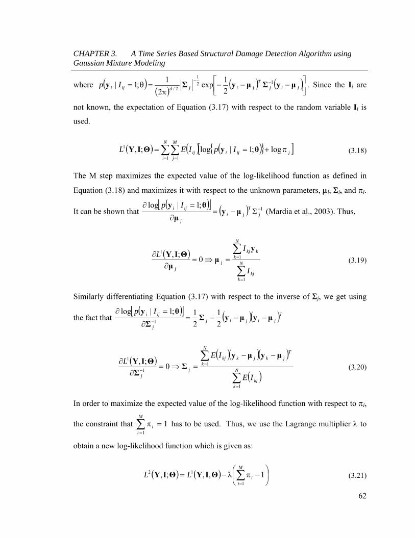
CHAPTER 3. A Time Series Based Structural Damage Detection Algorithm using Gaussian Mixture Modeling
62
where
jijT
jijdiji Ip μyΣμyΣy 12
1
2/ 2
1exp
2
1;1| . Since the Ii are
not known, the expectation of Equation (3.17) with respect to the random variable Ii is
used.
jiji
N
i
M
jij IpIEL
log;1|log;,1 1
1 θyΘIY (3.18)
The M step maximizes the expected value of the log-likelihood function as defined in
Equation (3.18) and maximizes it with respect to the unknown parameters, i, i, and i.
It can be shown that 1
;1|log
j
Tji
j
iji Ipμy
μ
θy (Mardia et al., 2003). Thus,
N
kkj
N
kkkj
jj I
IL
1
11
0;,
yμ
μ
ΘIY (3.19)
Similarly differentiating Equation (3.17) with respect to the inverse of j, we get using
the fact that Tjijij
j
iji IpμyμyΣ
Σ
θy
2
1
2
1;1|log1
N
kkj
N
k
Tjkjkkj
jj IE
IEL
1
11
1
0;,
μyμyΣ
Σ
ΘIY (3.20)
In order to maximize the expected value of the log-likelihood function with respect to i,
the constraint that
M
ii
1
1 has to be used. Thus, we use the Lagrange multiplier to
obtain a new log-likelihood function which is given as:
1,,;,1
12M
iiLL ΘIYΘIY (3.21)

CHAPTER 3. A Time Series Based Structural Damage Detection Algorithm using Gaussian Mixture Modeling
63
Differentiate (3.21) with respect to i, we get the following
NIEIE
MjIE
MjYLL
M
j
N
kkj
M
j
M
jj
N
kkj
j
N
kkj
jj
1 11 11
1
12
0
,...,1 0
,...,1 0;,;, ΘIΘIY
(3.22)
N
IEN
kkj
j
1
(3.23)
The E-step is now explained. It should be checked whether maximizing the log-
likelihood function L1(Y, I; ) is equivalent to maximizing the log-likelihood function of
the observed data, L(Y; ). This can be achieved by taking the expectation of Iij with
respect to the posterior probability density function of I, p(I| Y; ) (Bilmes, 1998).
M
kkiki
jiji
iijiijij
Ip
Ip
IpIpIE
1
;1
;1
;00;11
θy
θy
θyθy
(3.24)
The proof of the above is given as follows.
IIIIX
II
II
I
I
I
ΘIY
II
ΘIYIIΘIYΘY
II
dffL
df
Ypf
f
YpE
f
pE
df
pfdpp
ff
log;,
;,
log
Inequality sJensen' ;,
log;,
log
;,log;,log;log
1
(3.25)

CHAPTER 3. A Time Series Based Structural Damage Detection Algorithm using Gaussian Mixture Modeling
64
where Ef(I) is the expectation with respect to f(I). The second term in Equation (3.25) does
not depend on , and thus it suffices to maximizing L1(Y, I; ), which is what is done in
the M-step. As in the E-step, use f(I) = p(I| Y; ),
ΘYIΘYΘYI
IΘYI
ΘIYΘYII
I
ΘIYI
;log;log;
;
;,log;
;,log
pdpp
dp
ppd
f
pf
(3.26)
Thus, the lower bound in Equation (3.25) becomes an equality and thus validates both the
E and M steps.

65
Chapter 4
Damage Feature Extraction from Wavelet Transform of Vibration Signals
Chapters 2 and 3 presented damage detection algorithms that utilized autoregressive (AR)
coefficients as feature vectors. These algorithms are valid for stationary signals obtained
from linear systems. In order to enable damage detection with non-stationary signals, the
wavelet transform is used in this chapter to formulate a feature vector.
In the context of SHM, earlier work was carried out in wavelet based system
identification of non-linear structures by Staszewski (1998), Ghanem and Romeo (2000)
and Kijewski and Kareem (2003). From a signal processing viewpoint, initial work done
was by Hou et al. (2000), where the discrete wavelet transform is used to study the
transient phenomenon when the stiffness of the structure is abruptly changed. Sun and
Chang (2002) have used the wavelet packet transform for decomposition of the signals,
where the wavelet packet component energies are utilized to detect damage and are
inputs to a neural network for damage assessment.
CHAPTER 4. Damage Feature Extraction from Wavelet Transform of Vibration Signals
66
In this chapter, a damage sensitive feature based on the energies of the Haar and Morlet
wavelet transforms of the vibration signal is derived. The reason these wavelet bases are
selected is because these bases have closed form expressions and aid in the ease of
mathematical derivation. However any appropriate wavelet basis can be used. For
example, in the next chapter, the Daubechies wavelet with four filter coefficients (DB4)
wavelet coefficients is used for feature extraction.
In the first part of this chapter, the theoretical aspects of wavelet decomposition of
vibration signals are discussed. The continuous wavelet transform of a signal is written in
terms of the Fourier transform of the signal and the wavelet basis. In the second part, this
framework is used to derive a closed form expression for the energies of the Haar and
Morlet wavelet for a single degree and multiple degree of freedom systems. The
relationship of the damage sensitive feature to physical parameters of the structure such
as mode shapes, stiffnesses and damping ratios is demonstrated. In order to illustrate this
wavelet based method for damage detection, it is applied to the ASCE Benchmark
Structure. The effect of noise on these datasets is also studied.
4.1 Properties of the Continuous Wavelet
Transform
A wavelet is a function (t)L2() (the space of square integrable functions) with the
following properties (Mallat, 1999):
1
0
dtt (4.1)
The mother wavelet function (t)L2() that is dilated/scaled by a and translated by b,
denoted by a,b(t) and is given as
CHAPTER 4. Damage Feature Extraction from Wavelet Transform of Vibration Signals
67
a
bt
atba
1, (4.2)
where 1, ba . Then the continuous wavelet transform (CWT) of a function f(t)L2()
is given as:
dta
bt
atfbaWf
*
1, (4.3)
where * represents the complex conjugate. It should be noted that Equation (4.3) is a
convolution integral.
The main advantage of wavelet analysis over conventional spectral methods such as
Fourier methods is that data are localized in both time and scale domains (Mallat, 1999).
At lower scales, the wavelet basis function has a smaller support and thus is better able to
localize transient phenomena such as discontinuities in the dataset. Similarly, at higher
scales, the wavelet basis function has a wider support which helps in identifying long
range phenomena.
In the context of this study, it is useful to develop the wavelet transform in terms of the
Fourier Transform (FT) of a function rather than the function itself. Thus we define the
Fourier Transform of f(x) L2() as (Bracewell, 2000):
dtjtsxpetfsF
(4.4)
where, j is the square root of -1. The Inverse Fourier Transform (IFT) of F(s) is obtained
from
dsjtsxpesFtf
2
1 (4.5)
The Power Theorem is applied to obtain: (Bracewell, 2000)

CHAPTER 4. Damage Feature Extraction from Wavelet Transform of Vibration Signals
68
dsssFdtttf baba
,, 2
1 (4.6)
where (s) is the FT of (t).
By substituting Equation (4.6) in Equation (4.3), it follows that
dsssFbaWf ba
,2
1, (4.7)
The Fourier Transform a,b(s) of the wavelet function a,b(t), is obtained as follows
asjsbadtjtsa
bt
a
dtjtsts baba
expexp1
exp,,
(4.8)
Thus, substituting Equation (4.8) in Equation (4.7), Equation (4.7) is rewritten as:
dsasjsbasFbaWf
exp
2
1, (4.9)
In this study, the Haar wavelet and the Morlet wavelet bases are considered. Close
investigation of these wavelets will provide a physical understanding of wavelet
coefficients of an acceleration signal and will provide a basis for correlating these
coefficients to damage sensitive features in a pattern classification scheme. The reason
why the Haar and Morlet bases are chosen is because these wavelets have a closed form
expression and are thus more convenient for mathematical derivations.
For the purposes of applying a statistical pattern classification method for damage
detection, we define the energy of the wavelet coefficients at appropriate scales as the
damage sensitive feature. Thus, the energy of the wavelet coefficients at scale a, Ea, is
defined as follows:
K
ba baxWE
1
2, (4.10)
CHAPTER 4. Damage Feature Extraction from Wavelet Transform of Vibration Signals
69
where, baxW , is the wavelet coefficient of the acceleration signal at the ath scale and bth
time step, K is the number of data points in the signal and || is the absolute value of the
quantity.
In this study, damage detection is carried out by using the energy of the coefficients of
the sixth dyadic scale for the Haar wavelet, and the seventh dyadic scale for the Morlet
wavelet basis. Selection of these scales has to do with the support of the scaled wavelet
basis. The higher scales have larger support of wavelet basis, thus increasing the
likelihood of detecting long term changes. This implies that the wavelet coefficients at
higher scales would contain information about vibration modes at lower natural
frequencies. Since damage generally affects lower modes of vibration, these wavelet
coefficients at higher scales would be useful in damage detection. Also, at higher scales,
the wavelet coefficients do not pick up transient phenomenon such as spikes and jumps,
thus eliminating problems with noisy data.
In the following subsections we use the Fourier Transform of the Haar and Morlet
wavelets bases to derive the wavelet coefficients of a function f(t).
4.1.1 Haar Wavelet
The Haar wavelet is defined as follows:
0.15.0for 1
5.00for 1
t
tt (4.11)
The FT of the Haar wavelet can be shown to be equal to:
2
2exp1
1
js
jss (4.12)

CHAPTER 4. Damage Feature Extraction from Wavelet Transform of Vibration Signals
70
Thus, from Equations (4.9) and (4.12), the wavelet coefficients using the Haar basis is
given as:
dsjas
jsbs
sF
a
jbafWH
2
2exp1exp
2,
(4.13)
The Haar wavelet and its Fourier transform are shown in Figure 4.1.
4.1.2 Morlet Wavelet
The Morlet wavelet is defined as follows:
2expexp
2
0
ttjt (4.14)
The FT of the Morlet wavelet can be shown to be equal to:
2
02
1exp2 ss (4.15)
In general, the value of 0 is chosen to be 5, which satisfies the admissibility condition
(Mallat, 1999). Thus, from Equations (4.9) and (4.15), the wavelet coefficients using the
Morlet basis are given as:
dsasjsbasFbafWM
252
1expexp
2
1, (4.16)
The Morlet wavelet and its Fourier transform are shown in Figure 4.2.

CHAPTER 4. Damage Feature Extraction from Wavelet Transform of Vibration Signals
71
4.2 Derivation of the Damage Sensitive Feature
using Wavelet Coefficients of Acceleration
Signals for a SDOF System
Consider a single degree of freedom (SDOF) system, with mass m, damping coefficient c
and undamaged stiffness coefficient k, subject to a forcing function g(t) whose equation
of motion is given as:
tgkxxcxm (4.17)
Taking the Fourier transform of Equation (4.17) and applying the derivative rule
sFjsdt
tfdF n
n
n
the following expression is obtained:
sGsXkjcsms 2 (4.18)
where X(s) and G(s) are the FT’s of the displacement and forcing function respectively.
Here, we have made the assumption that the system is linear and the forcing function is
stationary. The first assumption is valid, since when we compare the damage with
undamaged system we are looking at an equivalent linear system with reduced stiffness.
The second assumption is not always valid in practice; however we can segment the
signal so that each signal is quasi-stationary.
With these assumptions, we can estimate the FT of the acceleration as:
kjcsms
sGssXstxFTsX
2
22 (4.19)
Using the framework developed in Sections 4.1.1, 4.1.2 and Equation (4.19), expressions
for the wavelet transform of acceleration signals is derived next.

CHAPTER 4. Damage Feature Extraction from Wavelet Transform of Vibration Signals
72
t
ψ(t
)
(a)
(b)
Figure 4.1: Haar Wavelet (a) Haar Basis Function and (b) its Fourier Transform
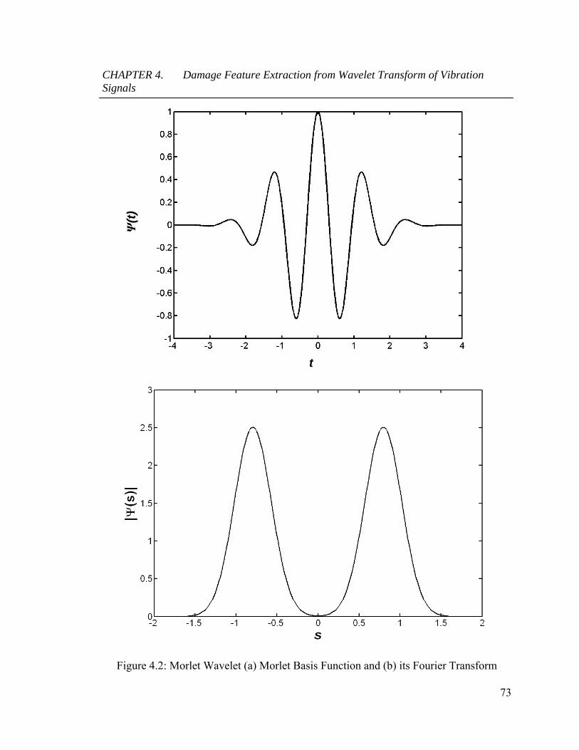
CHAPTER 4. Damage Feature Extraction from Wavelet Transform of Vibration Signals
73
t
Ψ(t
)
Figure 4.2: Morlet Wavelet (a) Morlet Basis Function and (b) its Fourier Transform
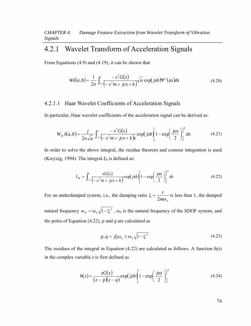
CHAPTER 4. Damage Feature Extraction from Wavelet Transform of Vibration Signals
74
4.2.1 Wavelet Transform of Acceleration Signals
From Equations (4.9) and (4.19), it can be shown that
dsasjsba
kjcsms
sGsbaxW
exp
2
1,
2
2
(4.20)
4.2.1.1 Haar Wavelet Coefficients of Acceleration Signals
In particular, Haar wavelet coefficients of the acceleration signal can be derived as:
2exp1exp
2,
2
2
2
dsjas
jsbskjcsms
sGs
a
jbaxWH
(4.21)
In order to solve the above integral, the residue theorem and contour integration is used
(Kreyzig, 1994). The integral IH is defined as:
ds
jasjsb
kjcsms
ssGI H
2
2 2exp1exp
(4.22)
For an underdamped system, i.e., the damping ratio nm
c
2is less than 1, the damped
natural frequency 21 nd , n is the natural frequency of the SDOF system, and
the poles of Equation (4.22), p and q are calculated as
21, nnjqp (4.23)
The residues of the integral in Equation (4.22) are calculated as follows. A function h(z)
in the complex variable z is first defined as
2
2exp1exp
jazjzb
qzpz
zzGzh (4.24)

CHAPTER 4. Damage Feature Extraction from Wavelet Transform of Vibration Signals
75
It can be proved that h(z) is analytic everywhere in the complex plane except at z = p and
z = q. Note that h(z) is analytic at z =0, since
2exp1
jaz is analytic at z =0. Using the
residue theorem, it can be shown that
qpH RRjI 2 (4.25)
where Rp and Rq are the residues of h(z) evaluated at p and q respectively. This proof of
Equation (4.25) is included in Section 4.6. Rp is given as:
;2
exp1exp
lim
2
qp
japjpbppG
zhpzR pzp
(4.26)
Similarly Rq is derived as
pq
jaqjqbqqG
Rq
2
2exp1exp
(4.27)
Here we assume that the G(s) is defined on the complex plane. Using the residue
theorem, it can be shown that
qpH RRa
baxW 1
, (4.28)
It is noted the residues Rp and Rq are related to the physical parameters of the system n
and ξ; and also on the loading on the SDOF system.
4.2.1.2 Morlet Wavelet Coefficients of Acceleration Signals
Using Equations (4.16) and (4.20), the Morlet wavelet transform of acceleration signals
may be derived as:

CHAPTER 4. Damage Feature Extraction from Wavelet Transform of Vibration Signals
76
2
1expexp
2, 2
02
2
dsasjsbkjcsms
sGsabaxWM
(4.29)
In a similar fashion to the previous subsection, the integral IM is defined as follows:
dsasjsb
kjcsms
sGsI M
202
2
2
1expexp (4.30)
The residues of the integral IM are given in Equation (4.23). A function h(z) in the
complex variable z is first defined as
2
0
2
2
1expexp azjzb
qzpz
zGzzh (4.31)
It can be proved that h(z) is analytic everywhere in the complex plane except at z = p and
z = q. Using the residue theorem, it can be shown that IM = 2j(Rp+Rq), where Rp and Rq
are the residues of h(z) evaluated at p and q respectively. Rp is given as:
;2
1expexp
lim
20
2
qp
apjpbpGpzhpzR pzp
(4.32)
Similarly Rq is derived as
pq
aqjqbqGqRq
20
2
2
1expexp
(4.33)
Here we assume that the G(s) is defined on the complex plane. Using the residue
theorem, it can be shown that
qpM RRjabaxW 2, (4.34)
With Equation (4.34), it is demonstrated that the wavelet coefficients of the acceleration
contain information about the physical parameters of the system. From Equations (4.28)

CHAPTER 4. Damage Feature Extraction from Wavelet Transform of Vibration Signals
77
and (4.34), we can derive the energy of the wavelet coefficients as defined by Equation
(4.10).
4.2.2 Damage Sensitive Feature
In this section, the damage sensitive feature is derived for a SDOF system using the Haar
and Morlet bases.
4.2.2.1 Haar Basis
Using the relationship
*22*2Re2
11, qpqpqpqpH RRRR
aRRRR
abaxW (4.35)
where Re() is the real part of the complex quantity, we can conclude that
*2222
1, qpqpH RRRR
abaxW (4.36)
It is noted that |p| = |q| = n. Also, we observe that
n
nnd
bjqb
bbjbjpb
expexp
expexpexpexp (4.37)
and
2
1
2
22
2exp1
2exp
2exp1
2exp1
2exp1
dnd jac
aja
japjap
(4.38)
Similarly, it is observed that

CHAPTER 4. Damage Feature Extraction from Wavelet Transform of Vibration Signals
78
2
2
22
2exp1
2exp
2exp1
2exp1
dnd ja
cajajaq
(4.39)
where
2
exp1
21
na
cc .
The coefficient c1 is a decreasing term in a, whereas c2 is an increasing term in a. Since
we consider higher scales to compute the energies, Equations (4.38) and (4.39) can be
approximated as follows:
22
2
2
1121
2
1
12
exp1
2cos21
2cos21
2exp1
cja
c
ac
acc
jac
d
ddd
(4.40)
Thus, using Equations (4.37) and (4.40) we can conclude that
2
222
22
1
2
22
14
12
cos212exp
cqGa
cpGb
RR
dn
qp (4.41)
In a similar fashion, we can show that
2
2
22
*
*
14
1
cqGpGRR qp (4.42)
The expression in Equation (4.42) is a constant (i.e., not a function of b) and thus is not
included in Equation (4.43).
2
222
22
1
2
2
14
12
cos212exp
,
a
cqGa
cpGb
baxW
dn
H (4.43)

CHAPTER 4. Damage Feature Extraction from Wavelet Transform of Vibration Signals
79
where
2
exp1
21
na
cc . For an acceleration signal sampled at 1/t Hz with K data
points, the energy at scale a for the Haar basis, EaHaar, is derived using Equation (4.43)
t
tKta
ba
cqGa
cpG
E
n
nnHaar
K
bn
d
Haara
2exp1
2exp12exp
2exp14
12
cos21
12
222
22
1
2
(4.44)
where
2
222
22
1
2
14
12
cos21
a
cqGa
cpG
a
d
Haar .
Equation (4.44) consists of Haar, which is a function of c1 and c2. Since the damage
sensitive feature is obtained at higher scales (i.e., the value of a increases) the value of c1
is not significant. As the extent of damage increases, the values of c1 increases and c2
decreases. In such cases, c2 will dominate, thus EaHaar is sensitive to damage at higher
scales.
4.2.2.2 Morlet Basis
Using similar principles as given in Equations (4.34) and (4.35),
*222
22, qpqpM RRRRabaxW (4.45)
It is noted that |p| = |q| = n. Also, we observe that
22222 21
2
1exp
2
1exp napa
dapa 00 expexp
(4.46)

CHAPTER 4. Damage Feature Extraction from Wavelet Transform of Vibration Signals
80
From Equation (4.46), we obtain
dn aa
papaap
020
222
020
2220
exp2
1exp21
2
1exp
exp2
1exp
2
1exp
2
1exp
(4.47)
Similarly, it is observed that
22222 21
2
1exp
2
1exp naqa
daqa 00 expexp
(4.48)
From Equation (4.48), we obtain
dn aa
qaqaaq
020
222
020
2220
exp2
1exp21
2
1exp
exp2
1exp
2
1exp
2
1exp
(4.49)
Thus, using Equations (4.32), (4.33), (4.47) and (4.49) and we can conclude that
2
1
2
122
02222
22
14
21exp2exp
d
qGdpGab
RR
nnn
qp (4.50)
where, d1 = exp(2a0d). In a similar fashion, it is shown that
2
20
2222*
*
14
21exp
nn
qp
aqGpGRR (4.51)
Since Equation (4.51) is not a function of b,

CHAPTER 4. Damage Feature Extraction from Wavelet Transform of Vibration Signals
81
2
1
2
122
02222
2
12
21exp2exp
,
d
qGdpGab
abaxW
nnn
M (4.52)
Thus, the energy of the Morlet based wavelet coefficients of the acceleration signal at
scale a, EaMorlet, is derived in a similar fashion and is given as follows:
t
tKtaE
n
nnMorl
Morleta
2exp1
2exp12exp (4.53)
where, 0 = 5,
2
1
2
122
02222
12
21exp
d
qGdpGa
aa
nn
Morl and d1=
exp(2a0d).
Assuming a constant value of (say, = 0.1), it is observed that d1 increases with
increases in the value of a. Also d1, which is a function of the damped natural frequency,
decreases with increase in the extent of damage. Since EaMorlet is a function of d1 and n,
both of which decrease with an increase in damage extent, EaMorlet is a good indicator of
damage. It should be noted that Ea is also a function of the loading.
4.3 Derivation of the Damage Sensitive Feature
using Wavelet Coefficients of Acceleration
Signals for a MDOF System
We next consider a structural system with N degrees of freedom (dof) with M, C and K
defined as the mass, damping and stiffness matrices (of size NN), respectively. The
forcing function is denoted by g(t). For a proportionally damped system and assuming
that the damping ratio in each mode is equal to , the transfer function of the

CHAPTER 4. Damage Feature Extraction from Wavelet Transform of Vibration Signals
82
displacement at the kth dof xk(t) and the forcing function at the lth dof, Hkl(s), can be
derived as (Maia and Silva, 1998):
N
r rr
lrkr
l
kkl sjssG
sXsH
122 2
(4.54)
where Xk(s) and Gl(s) is the Fourier transform of the displacement at the kth dof xk(t) and
the forcing function at the lth dof gl(t). Thus, the FT of the acceleration txk is given as:
N
r rr
llrkrk sjs
sGssX
122
2
2 (4.55)
where r is the rth modal natural frequency, kr and lr are the kth and lth elements of the
mass normalized rth mode shape vector r. Using similar principles utilized in Section
4.2, the wavelet coefficients of a MDOF system are derived in the next subsection.
4.3.1 Wavelet Coefficients of Acceleration Signals
With respect to the Haar wavelet, the wavelet coefficient of the acceleration txk is
derived as:
ds
jasjsb
sjs
sGs
a
jbaxW
N
r rr
llrkrkH
2
122 2
exp1exp22
,
(4.56)
In order to calculate the above integral, we will use principles of contour integration as is
done for SDOF systems presented in the previous section. Again, the integral Ir for the rth
vibration mode, is defined as:
dsjas
jsbsjs
sGsI
rr
llrkrr
2
22 2exp1exp
2 (4.57)
The poles of Equation (4.57), p1,r and p2,r are calculated as

CHAPTER 4. Damage Feature Extraction from Wavelet Transform of Vibration Signals
83
2
,2
,1 1
rr
r
r jp (4.58)
The function t(z) in the complex variable z defined as
2
21 2exp1exp
jaz
jzbpzpz
zzGzt llrkr (4.59)
It can be proven that t(z) is analytic everywhere in the complex plane except at z = p1,r
and z = p2,r. Using the residue theorem, it can be shown that Ir = 2j(R1,r+R2,r), where R1,r
and R2,r are the residues of t(z) evaluated at p1,r and p2,r respectively. R1,r and R2,r are
evaluated as:
;2
exp1exp
lim,2,1
2
,1,1,1,1
,1,1 ,1
rr
rrrlrlrkr
rpzr pp
japbjppGp
ztpzRr
(4.60)
Similarly R2,r can be derived as
rr
rrrllrkr
r pp
japbjppGp
R,1,2
2
,2,2,22
,2
2exp1exp
(4.61)
Using the residue theorem, it can be shown that
N
rrrH RR
abaxW
1,2,1
1, (4.62)
Again, we approximate the energy of the Haar wavelet coefficients of acceleration txk
at scale a as
N
rrr
Haarka RR
aE
1
2
,2
2
,1,
1. The rth damped natural frequency d,r is
given as: 2, 1 rrd . We define
2
exp1
,2,1
r
rr
a
cc .

CHAPTER 4. Damage Feature Extraction from Wavelet Transform of Vibration Signals
84
Using similar approximations as in the previous section, we obtain the following
expression for HaarkaE , as:
K
b
N
r
rlrd
rlrlrkr
Haara a
cpGa
cpGb
E1 1
2
222
2
,2
2
,1
2
,122
14
12
cos212exp
(4.63)
Interchanging the summations, we can derive that
N
r r
rrlrkrHaar
Haara t
tKtraE
1
22
2exp1
2exp12exp, (4.64)
where
2
22,2
2
,2
2
,,1
2
,1
14
12
cos21
,
a
cpGa
cpG
ra
rrlrd
rrl
Haar .
The energy of the Morlet based wavelet coefficients of acceleration txk at scale a,
EaMorlet, is derived in a similar fashion and is given as follows:
N
r r
rrlrkrMorl
Morleta t
tKtraE
1
22
2exp1
2exp12exp, (4.65)
where 0 = 5,
2
,1
2
,122
02222
12
21exp
,
r
rrr
Morl
d
qGdpGa
ara and d1,r =
exp(2a0d,r).
It is again observed that the energies of the wavelet coefficients for both the Haar and
Morlet wavelet basis contain information of the physical system. Ea contains modal
information of the system through the kth and lth mass normalized eigen vectors k and
l. In the case of EaHaar, as the extent of damage increases and which mode is excited due
to the increase in damage, c1,r increases and c2,r decreases. As the value of a increases, the
CHAPTER 4. Damage Feature Extraction from Wavelet Transform of Vibration Signals
85
value of c1,r is not significant. In such cases, c2,r will dominate. In the case of EaMorlet,
assuming a constant value of the damping ratio = 0.1, it is observed that d1,r increases
with an increase in the value of a. Also d1,r reduces with increase in the extent of damage
depending on which mode is excited due to the damage. Thus Ea can be used as an
indicator of damage.
Thus, it can be concluded that as the stiffness decreases due to damage, the response of
the structure will change resulting in changes of energies of the wavelet coefficients.
Consequently, the damage sensitive feature based on the wavelet coefficients can capture
this change in measurements from an undamaged to damaged structural state.
4.4 Application
In order to test the validity of the above derived damage sensitive feature, numerically
simulated datasets from the ASCE Benchmark Structure have been used. The description
of the ASCE Benchmark Structure was provided in Chapter 2. Damage detection analysis
is performed with both the Haar and Morlet wavelet bases.
4.4.1 Damage Detection
Damage detection is performed under the premise that the damage sensitive feature will
migrate with the onset of damage. In this study, the damage sensitive feature is defined as
the energy of the wavelet coefficients at the seventh dyadic scale for the Morlet wavelet
(denoted by E7) and the sixth dyadic scale for the Haar wavelet (denoted by E6). The
reason for choosing the seventh dyadic scale for the Morlet wavelet is because this scale
is optimal for capturing important characteristics of the signal which are sensitive to
damage. It is noted that similar results are obtained for the fifth and sixth dyadic scales.

CHAPTER 4. Damage Feature Extraction from Wavelet Transform of Vibration Signals
86
The results of the studies for sensors 2, 3, and 9 are presented. First, results using the
Morlet wavelet basis are presented, followed by the Haar basis.
4.4.1.1 Sensor 2
Figure 4.3 show the migration of the features extracted from signals from sensor 2, from
an undamaged state to the damaged state for damage patterns 6 and 3. In the case of
damage pattern 6 (Figure 4.3(a)), where the stiffness of a brace is partially reduced on the
first floor, it is observed that there is a small separation between the means of E7.
However, this separation is larger for damage pattern 3 (Figure 4.3(b)), where a brace is
removed on the first floor. This difference in the means is significantly larger in the case
of major damage patterns 1 and 2 (Figure 4.4). It is also noted that the variance of the
clouds increase with increase in damage.
4.4.1.2 Sensor 3
Figure 4.5 illustrates the migration of E7, extracted from sensor 3 for damage patterns 4
and 5. The means of the damage sensitive feature E7 for the damaged clouds of damage
patterns 4 and 5 are 21.39 and 21.45 respectively. These results indicate that the change
due to bolt loosening was not detected.
4.4.1.3 Sensor 9
Figure 4.6 illustrates the feature clouds, extracted from sensor 9, for damage patterns 3
and 4. For damage pattern 3, it is observed that there is very little separation between the
clouds because the brace has been removed in the x direction and sensor 9 measures the
acceleration in the y direction (Figure 2.7). For damage pattern 4, there are two distinct
clouds of feature vectors with damage since a brace has been removed from the third
storey in the y direction near sensor 9.

CHAPTER 4. Damage Feature Extraction from Wavelet Transform of Vibration Signals
87
Similar results are obtained with the Haar wavelet for major damage patterns, but the
clouds do not show separation for minor damage patterns. The reason for this is that the
Haar wavelet is a simple wavelet (Figure 4.1) and thus may not be able to capture
important details of the vibration signal. Figure 4.7 - 4.10 illustrates the effectiveness of
the Haar wavelet in damage detection. It is noted that similar trends were observed for the
Haar wavelet at the fifth dyadic scale.
In the previous chapter, a damage extent measure was derived using the Mahalanobis
distance. The same measure DM is used in damage extent calculations and is defined as:
damagedundamagedundamagedT
damagedundamagedDM μμΣμμ 1 (4.66)
where undamaged is the covariance matrix of the undamaged dataset, undamaged and damaged,
are the means of the undamaged and damaged dataset respectively. Table 4.1 shows the
variation of DM (for the Morlet wavelet) for all sensors and various damage patterns.

CHAPTER 4. Damage Feature Extraction from Wavelet Transform of Vibration Signals
88
(a)
(b)
Figure 4.3: Migration of the Morlet wavelet based damage sensitive feature E7 for sensor 2 with damage for minor patterns (a) Damage pattern 6 and (b) Damage Pattern 3

CHAPTER 4. Damage Feature Extraction from Wavelet Transform of Vibration Signals
89
(a)
(b)
Figure 4.4: Migration of Morlet wavelet based damage sensitive feature E7 for sensor 2 with damage for major patterns (a) Damage pattern 1 and (b) Damage Pattern 2

CHAPTER 4. Damage Feature Extraction from Wavelet Transform of Vibration Signals
90
(a)
(b)
Figure 4.5: Migration of Morlet wavelet based damage sensitive feature E7 for sensor 3 with damage for (a) Damage pattern 4 and (b) Damage Pattern 5 (Undamaged ;
Damaged +)

CHAPTER 4. Damage Feature Extraction from Wavelet Transform of Vibration Signals
91
(a)
(b)
Figure 4.6: Migration of Morlet wavelet based damage sensitive feature E7 for sensor 9 with damage for (a) Damage pattern 3 and (b) Damage Pattern 4 (Undamaged ;
Damaged +)

CHAPTER 4. Damage Feature Extraction from Wavelet Transform of Vibration Signals
92
(a)
(b)
Figure 4.7: Migration of the Haar wavelet based damage sensitive feature E6 for sensor 2 with damage for minor patterns (a) Damage pattern 6 and (b) Damage Pattern 3

CHAPTER 4. Damage Feature Extraction from Wavelet Transform of Vibration Signals
93
(a)
(b)
Figure 4.8: Migration of the Haar wavelet based damage sensitive feature E6 for sensor 2 with damage for major patterns (a) Damage pattern 1 and (b) Damage Pattern 2

CHAPTER 4. Damage Feature Extraction from Wavelet Transform of Vibration Signals
94
(a)
(b)
Figure 4.9: Migration of the Haar wavelet based damage sensitive feature E6 for sensor 3 with damage for (a) Damage pattern 4 and (b) Damage Pattern 5 (Undamaged ;
Damaged +)

CHAPTER 4. Damage Feature Extraction from Wavelet Transform of Vibration Signals
95
(a)
(b)
Figure 4.10: Migration of the Haar wavelet based damage sensitive feature E6 for sensor 9 with damage for (a) Damage pattern 3 and (b) Damage Pattern 4 (Undamaged ;
Damaged +)

CHAPTER 4. Damage Feature Extraction from Wavelet Transform of Vibration Signals
96
Table 4.1: Variation of DM for the Morlet wavelet based damage sensitive feature for various sensors and different damage patterns
Sensor Damage Metric DM
DP1 DP2 DP3 DP4 DP5 DP6
1 9.68 21.52 0.85 0.95 0.95 0.33 2 99.63 146.00 7.71 7.49 7.49 1.63 3 9.12 18.43 0.98 2.57 2.57 0.35 4 97.10 123.32 5.89 5.58 5.58 1.33 5 5.85 10.96 1.27 1.49 1.49 0.39 6 62.01 72.05 6.70 6.60 6.60 1.46 7 7.13 12.65 1.87 2.13 2.13 0.39 8 63.94 80.00 4.66 4.55 4.55 1.08 9 6.18 11.35 0.95 6.65 6.65 0.25
10 50.89 43.29 5.46 5.49 5.49 1.52 11 5.54 9.51 1.22 5.49 5.49 0.25 12 53.05 43.02 5.02 5.06 5.06 1.11 13 3.12 8.12 0.97 1.60 1.60 0.27 14 48.64 43.83 5.74 5.52 5.52 1.29 15 4.53 10.89 1.06 1.48 1.48 0.24 16 40.76 41.20 3.87 3.90 3.90 0.88
From the analysis, the following observations are made
The values of DM are correlated to the amount of damage. As can be observed
from Table 4.1, the general trend for the damage metric DM is that it increases
for damage patterns 6, 3, 4, 5, 1 and 2, which corresponds to a progressive
increase in damage.
With regard to DP4 and DP5, there is no change in the values of the damage
measure, thus indicating that bolt loosening could not be detected.
4.4.1.4 Effect of Noise
The effect of zero mean additive Gaussian white noise on the damage detection algorithm
is studied. The ratio of the root mean square (rms) value of the noise to the rms value of

CHAPTER 4. Damage Feature Extraction from Wavelet Transform of Vibration Signals
97
the signal is defined as the noise to signal ratio, and is denoted as NSR. The NSR is
varied from 0.05 to 0.15. The values of DM with these noise levels for sensor 2 are
presented in Table 4.2.
Table 4.2: Variation of DM for sensor 2 with different noise to signal ratios (NSR) for damage patterns DP 1-6
NSR Damage Metric DM
DP1 DP2 DP3 DP4 DP5 DP6
0.0 103.26 151.25 7.87 7.66 7.66 1.68 0.5 57.00 78.17 2.11 1.84 1.84 0.36
0.10 20.11 35.16 0.88 0.53 0.53 0.00 0.15 10.49 17.13 0.22 0.46 0.46 0.00
From the analysis, the following observations are made:
The values of DM are correlated to the amount of damage. For damage
patterns 3 and 4, there is very slight difference between these values since at
sensor 2, DP 4 is DP 3 + removal of a brace in a direction perpendicular to the
direction of acceleration measured at sensor 2. Similar conclusions can be
made for DP 4 and DP 5.
The values of DM are sensitive to noise and only major damage patterns 1 and
2 can be detected at high ranges of noise levels
As expected, the separation of the clouds decreases with noise.

CHAPTER 4. Damage Feature Extraction from Wavelet Transform of Vibration Signals
98
4.5 Summary
In this chapter, a damage sensitive feature based on the wavelet transform of the vibration
signal is derived. The damage sensitive feature is defined as the energy of the wavelet
coefficients at higher scales. Theoretical aspects of wavelet decomposition of vibration
signals are presented. Expressions for the energies of wavelet coefficients using the Haar
and Morlet wavelet bases are derived for a single degree and multi-degree of freedom
system. The derived damage sensitive feature is applied to various datasets for the ASCE
Benchmark Structure using the Haar and Morlet wavelets. The effect of noise on these
datasets is also studied.
It is observed that the Haar wavelet is able to detect only major damage patterns. The
reason for this is that the Haar wavelet is a simple wavelet (Figure 4.1) and thus may not
be able to capture important details of the vibration signal. In comparison, the Morlet
wavelet performs much better and is able to detect minor damage patterns. Thus for
applications, it would be advisable to use energies of the Morlet wavelet coefficients at
higher scales.
The Morlet wavelet based energies at the seventh dyadic scale were able to detect
damage for major damage patterns at relatively high levels of noise. However, at higher
noise levels, minor damage patterns are not detected. The reason for this might be
because that the sensitivity of the loading at these scales might have dominated the
sensitivity of the damage on the damage sensitive feature. Thus, it would be critical to
perform normalization step of the damage diagnosis algorithm. This is discussed in
Chapter 5.
The proposed damage sensitive feature is shown to be effective in detecting damage for
numerically simulated datasets obtained from the ASCE Benchmark Structure.
Application of the damage sensitive feature to the ASCE Benchmark simulation
experiment demonstrates that the algorithm is able to detect minor, moderate and major

CHAPTER 4. Damage Feature Extraction from Wavelet Transform of Vibration Signals
99
damage patterns. However, loosening of bolts cannot be distinguished when it occurs in
conjunction with damage pattern 4. In general it would be difficult to detect bolt
loosening, unless a signal is obtained at the bolt itself and is used to identify damage.
With the acceleration measurements presented in the simulation experiment, highly
localized damage would be difficult to capture. It is also shown that the damage decision
for minor damage patterns is effected by high levels of noise.
4.6 Appendix: Derivation of the Integral IH
In this appendix, the derivation for the computation of Equation (4.22) is given.
p q
(R,0) A
B
C
(-R,0)
1R
2,R
Figure 4.11: Illustration of the Proof of the Contour Integration Formula

CHAPTER 4. Damage Feature Extraction from Wavelet Transform of Vibration Signals
100
Let the path R = 1,R + 2,R, where Figure 4.11 shows that 1,R is the arc ABC and 2,R is
the arc CA. If R is sufficiently large, the both poles p and q are within R. By the residue
theorem,
qp RRjdzzhR
2 (4.67)
where Rp and Rq are poles of the function h(z) and are given by Equation (4.26) and
Equation (4.27) respectively. In this section, we will show that 0lim,2
R
dzzhR
. For this
purpose, we prove the following Lemma.
Lemma: Let d > 0. Then, 0sinexplim0
ddRR
.
Proof:
2/
2/
00
sinexpsinexpsinexp ddRddRddR (4.68)
To compute the second integral, make the substitution = – . Thus,
2/
02/
sinexpsinexp
ddRddR (4.69)
Thus,
2/
00
sinexp2sinexp
ddRddR (4.70)
Now, choose an arbitrarily small > 0
2/
0
2/
0
sinexpsinexpsinexp
ddRddRddR (4.71)

CHAPTER 4. Damage Feature Extraction from Wavelet Transform of Vibration Signals
101
Since the function sinexp dR is decreasing in in [0,/2] and
sinexpsinexp dRdR in [ε,/2], we obtain
sinexp2
sinexp2/
dRddR (4.72)
If R is sufficiently large enough, i.e.,
2log
sin
1
dR , then
2/
sinexp ddR .
Thus, for any > 0, there exists R, such that if R > R,
2sinexp2/
0
ddR . Hence,
0sinexplim2sinexplim2/
00
ddRddRRR
(4.73)
Now on 2,R, z = Rexp(j), and [0,] and for any real valued a,
sinexpsinexpcosexpexp aRaRiRjaz (4.74)
Furthermore,
sinexpsin2
exp21
exp2
exp212
exp12
aRRa
jazjazjaz
(4.75)
Using the fact that dz = jRexp(j)d, we obtain
expexp
sinexpsin2
exp21sinexp
0,2
dqRjpRj
aRRa
bRzG
RdzzhR
(4.76)
Here again, we can approximate

CHAPTER 4. Damage Feature Extraction from Wavelet Transform of Vibration Signals
102
R
qRqRj
R
pRpRj 1exp;1exp (4.77)
Thus, for sufficiently large R, and say for some fixed constant , e.g., = 0.5, we get
4expexp
2
qRjpRj
R
(4.78)
Thus, Equation (4.76) maybe rewritten as
0
00
sinexp
sin2
exp2sinexp
exp4
,2 dRba
dRba
dbR
RjGR
dzzhR
(4.79)
By the Lemma, each of these integrals on the RHS of Equation (4.79) has to converge to
zero.
Thus, 0lim,2
R
dzzhR
Then,
R
R
HRR
IdzzhdzzhR
limlim
(4.80)
Thus, IH = 2j(Rp + Rq).

103
Chapter 5
A Wavelet Based Damage Detection Algorithm
In Chapter 4, a damage sensitive feature based on the energies of the wavelet transform
of the vibration signal was derived. In this chapter, a damage detection algorithm based
on this feature is presented. This algorithm requires the creation of a database of
normalized baseline signals. A methodology is developed for obtaining the best signal in
the database, closest to the new signal, using the lower singular values of the energies of
the wavelet coefficients at the first dyadic scale. To obtain the damage sensitive feature
vector, the energies of the wavelet coefficients at the fifth, sixth and seventh dyadic
scales are used. Principal components are used in this regard. Damage detection is
performed by using the k-means algorithm and the gap statistic. The k-means algorithm
estimates the cluster centers in a dataset and the gap statistic is used to determine the
optimal number of clusters in the dataset. It is hypothesized that more than one cluster is
an indication of change and this change is most likely due to damage. Finally, this
algorithm is tested using datasets from the ASCE Benchmark Structure.

CHAPTER 5. A Wavelet Based Damage Detection Algorithm
104
5.1 Overview of Algorithm
This algorithm requires creating a database of baseline measurements (which can include
accelerations and strains) and computing the coefficients of the continuous Daubechies
wavelet of order four (DB4) at appropriate scales. The DB4 wavelet is chosen because it
is similar to the Morlet wavelet and has a discrete wavelet counterpart which can be used
when embedding the algorithm at the sensor level. Following this, principal components
analysis is performed on the energies of the DB4 wavelet coefficients at the first dyadic
scale. This step helps in obtaining the closest signal in the database, which describes the
loading condition of the new signal. Once the closest baseline signal in the database is
chosen, feature vectors are calculated using the DB4 wavelet coefficients at the fifth,
sixth and seventh dyadic scales. Finally the k-means algorithm and the gap statistic are
used to discriminate between damaged and undamaged states in the structure. Damage is
detected when the algorithm predicts more than one cluster in the feature vectors under
question. The proposed detection algorithm is as follows:
i Obtain signals from an undamaged structure, from sensor i, denoted by xi(t) (i
= 1,…,P), where P is the number of sensors. Segment the signal xi(t) into
chunks of finite duration xij(t) (j = 1,…,Q ), where Q is the number of chunks.
Normalize these signals to obtain a mean zero and standard deviation one
signal as described in Equation (2.1). Populate the database with these
normalized baseline signals.
ii Compute the DB4 wavelet coefficients of the baseline signals at the first, fifth,
sixth and seventh dyadic scales. Calculate the norm of the wavelet coefficients
within a window size of size d = 20 data points. These are represented by
Qjjbaselinejbaselinejbaselinejbaselinejbaseline ,...,1 ,,7,,6,,5,,1, EEEEE (5.1)
where Ei,baseline,j is the energy vector of the wavelet coefficients of the jth
baseline signal at the ith dyadic scale. It is noted that Ei,baseline,j (i = 1, 5, 6, 7; j
CHAPTER 5. A Wavelet Based Damage Detection Algorithm
105
= 1,…,Q) is a vector of dimension K/d 1, where each baseline signal is of
length K.
iii Obtain the new signal at a later time, say t. This new signal could be obtained
from a potentially damaged location.
iv Compute the DB4 wavelet coefficients of the new signals at the first, fourth,
fifth and sixth dyadic scales. Energies of these coefficients are calculated in a
similar fashion as performed in step ii. These are represented by
Qjjnewjnewjnewjnewnew ,...,1 ,,7,,6,,5,,1 EEEEE (5.2)
where Ei,new,j is the energy of the wavelet coefficients of the jth chunk of the new
signal at the ith dyadic scale.
v Selection of closest baseline signal step: Search for the best baseline signal
(obtained in Step i) with similar environmental and loading conditions. This is
performed as follows:
For each baseline signal, form a matrix Z0,j = [E1,baseline,j E1,new,j] (j =
1,…,Q) of dimension K/d 2.
Perform a principal components (PC) analysis on Z0, j.
Obtain the principal direction, v1j (j = 1,…,Q). Also, obtain the minimum
variance (square of the lowest singular value) and denote it as 0j.
Choose the signal closest to the new signal as that signal with the value of
1,21
,11 j
jj v
v and the lowest value of 0j, where v11,j and v21,j are the
values of the components of vector v1j.

CHAPTER 5. A Wavelet Based Damage Detection Algorithm
106
vi Feature extraction step: Extract features by comparing the energies of the new
signal with that of best signal. This is performed as follows:
Form a matrix Zj,k = [Ei,best,j Ei,new,j] (i = 5,6,7; j = 1,…,Q; k = 1,2,3), where
Ei,best,j is the energy of the wavelet coefficients of the jth chunk of the best
signal in the database at the ith dyadic scale.
Perform a principal component analysis on Zj,k (j = 1,…,Q; k = 1,2,3).
Obtain the minimum variance (square of the lowest singular value) and
denote it as j,k (j = 1,…,Q; k = 1,2,3).
Choose the damage sensitive feature vector as = [1 2 3] where 1 is
the vector whose jth component is j,1.
vii Classification step: Use the k-means clustering algorithm with the gap statistic
to discriminate between a damaged state and an undamaged state.
Fix the number of clusters as k. For a fixed value of k, obtain the cluster
centers of the grouped feature vectors X defined in Equation (5.3), using
the k-means algorithm.
new
undamaged
κ
κX (5.3)
where undamaged and new are the feature vectors obtained from an undamaged
and new signal respectively. Calculate the gap statistic (Tibshirani et al.,
2001).
Use the gap statistic to determine the optimal number of clusters. If the
number of clusters is greater than one, then it is hypothesized that some
degree of damage has taken place. If, however, the clusters are very close

CHAPTER 5. A Wavelet Based Damage Detection Algorithm
107
based on the gap statistic, then it is concluded that there is no damage.
Such signals would be stored in the baseline database.
viii If there is damage, calculate the extent of damage by using the Euclidean
distance between the means of the damaged and undamaged clusters.
ix Go to step iii.
5.2 Application of Principal Components Analysis
in Optimal Selection of Baseline Signal and
Feature Extraction
In order to perform steps (v) and (vi), principal components analysis will be used. The
theory of principal components analysis is explained below.
5.2.1 Principal Components Analysis
Principal components analysis is a linear transformation used in multivariate statistical
analysis, generally used to reduce the dimension of the dataset and to find patterns (or
feature extraction) in the dataset (Mardia et al., 2001). The mathematical principle behind
PCA is explained as follows: Consider a mean centered matrix Y of dimension, say Np.
The sample covariance matrix is given by S = YTY/N-1. Then the eigen decomposition of
YTY is given as
p
p
TT
ddddiag ,...,,
...
21
21
2
D
vvvV
VVDYY
(5.4)

CHAPTER 5. A Wavelet Based Damage Detection Algorithm
108
where, V is a set of eigenvectors vi (i =1,..,p) and D is the singular value matrix. The
eigenvectors vj are called the principal components directions of Y. The first principal
component z1 = Yv1 has the largest sample variance amongst all the linear combinations
of the columns of Y (Mardia et al., 2001). In this study, principal components (PC’s) are
not used to reduce dimensionality but are used for feature extraction.
5.2.2 Selection of the Closest Baseline Signal
In practice, vibration data are collected under different operational conditions (loading
amplitude and direction; and environmental conditions such as temperature and
humidity). In order to compare ambient (or linear) vibration signals under various
operational conditions, we will use the energies of the wavelet coefficients at the 1st
dyadic scales to determine whether there is any difference in the loading conditions of the
signal or not. The reason why lower scales are chosen is that the wavelet coefficients at
these scales will be able to take into account the transient phenomenon such as jumps and
spikes and thus describe the loading conditions better.
Figure 5.1 illustrates the plot of the energies of the wavelet coefficients at the first dyadic
scale, for a similar and dissimilar vibration signal. The vector v1 is plotted at 45o to the x
axis. In the case when we obtain acceleration datasets from similar loading conditions, it
is noticed that the clouds cluster along the direction of v1. The reason for this is that these
values of E1,baseline,j and E1,new,j should be similar and thus cluster around v1, implying a
low variance in the direction of v2. The best signal in the database closest to the new
signal is selected using the following procedure:
Form the matrix Z0,j = [E1,baseline,j E1,new,j] (j = 1,…,Q). Perform a principal
component analysis on Z0,j.

CHAPTER 5. A Wavelet Based Damage Detection Algorithm
109
jj
j
jjj
Tjjjj
Tj
dddiag
Qj
21
21
2,0,0
,
,...,1
D
vvV
VDVZZ
(5.5)
where, Vj is a set of eigenvectors and Dj is the singular value matrix, obtained from
the decomposition of Z0,j.
Obtain the principal directions v1j to calculate the ratio j
jj v
v
,21
,11 and 22,0j
j d
(j=1,…,Q). Among all the signals in the database, find that signal in the database
with the values of the ratio j approximately equal to one and having the lowest
value of 0,j.
E 1, baseline,1
Similar signal
Dissimilar signal
E 1 , new,1
v 1
v 1 ’
v 2
v2 ’
Figure 5.1: Illustration of a similar and dissimilar cloud by comparing E1,baseline and E1,new

CHAPTER 5. A Wavelet Based Damage Detection Algorithm
110
In the case when the signals are not similar, the value of E1,new,1 and E1,baseline,1 would be
different and thus deviate away from the vector v1. Also, the variance (spread) in the
direction v2 would give an indication of similarity. To this end, the principal directions
will be used to obtain the directions of highest variances. The variance in the direction of
the second principal direction is used to show how dissimilar the signals are. This is
denoted as 0, whose jth component is 0,j. Thus, the lower the value of 0,j, more similar
the signals are. The reason why the first scale is chosen is because the coefficients at the
first scale will be able to detect transient phenomenon, which is a good descriptor of
loading conditions. This assumes that damage does not the affect the higher frequency
modes of vibration.
Figure 5.2 illustrates the comparison of two loading conditions as defined in the ASCE
Benchmark Structure Experiment. The first excitation is a series of independent filtered
Gaussian white noise loads generated using a sixth - order low-pass Butterworth filter
with a 100 Hz cutoff and applied at each story of the structure. The second loading is a
random excitation generated by a shaker on the roof-top of the center column.
Figure 5.2(a) shows the histogram of when comparing an acceleration signal from
sensor 2 for damage pattern 2 to baseline signals recorded for the same loading
conditions. The values of are in the range of 0.8-1.6, indicating that loading conditions
are similar. Also it is noted that even though damage pattern 2 is the most severe of the
damage patterns, it does not affect the values of .
Similarly, Figure 5.2(b) shows the histogram of when comparing an acceleration signal
from sensor 2 for an undamaged signal with baseline signals recorded for different
loading conditions. The values of are much higher than one and are in the range of 4.0-
6.0, indicating that loading conditions are not similar.

CHAPTER 5. A Wavelet Based Damage Detection Algorithm
111
(b)
(a)
Figure 5.2: Histogram of for sensor 2 for (a) similar loading condition with DP2 and (b) dissimilar loading conditions for undamaged cases

CHAPTER 5. A Wavelet Based Damage Detection Algorithm
112
Number of records
κ 0
Figure 5.3: Variation of 0 for similar loading conditions comparing undamaged case and damage pattern 2
Figure 5.3 shows the variation of 0 for similar loading conditions while comparing a
signal from sensor 2 and damage pattern 2 to a database of eighty similar baseline
signals. The lowest value of 0 is chosen as the best signal in the database, closest to the
new signal.
5.2.3 Feature Extraction
Figure 5.4 illustrates the feature extraction procedure. Values of the energies of the
wavelet coefficients at the fifth dyadic scale of the best baseline signal E5,best and the new
signal E5,new are compared. Principal components analysis (PCA) is performed on this
dataset and the variance in the second principal direction v2, denoted as 1, is chosen as

CHAPTER 5. A Wavelet Based Damage Detection Algorithm
113
the first element of the feature vector . Similarly 2 and 3 (second and third elements of
the feature vector) are derived using the energies at the sixth and seventh dyadic scales
respectively. Intuitively, it can be understood a large value of is a good indicator of
damage.
E5, best
Undamaged cloud
Damaged cloud
v3
v2
v4
E 5 , damaged
v 1
Figure 5.4: Illustration of damaged and undamaged cloud using principal components analysis
It should be noted that the fifth, sixth and seventh dyadic scales are chosen by trial and
error. Thus, when using this algorithm with a real structure, a finite element model of the
structure under question should be developed. Damage should then be induced on the
finite element model and the most sensitive scales can be chosen from a similar analysis
as stated in this section.

CHAPTER 5. A Wavelet Based Damage Detection Algorithm
114
Figure 5.5: Variation of the damage sensitive feature vectors for damage patterns (DP) 0, 1 and 6 as defined in the ASCE Benchmark Experiment
Figure 5.5 illustrates the variation of the damage sensitive feature for an undamaged case,
major damage pattern 1 and minor damage pattern 6. It is noted that the values of the
damage sensitive feature for an undamaged case are close to zero. However, for damage
patterns 1 and 6, the values of the feature vector are significantly greater than zero and
form separate clouds with respect to the undamaged cloud, thus indicating damage. From
Figure 5.5, it is also observed that as the level of damage increases the distance of the
cloud from the origin increases. In the next section, a classification methodology for
damage detection using the k-means algorithm and the gap statistic is explained. Also, a
damage measure DM using the Euclidean distance between the means of the undamaged
and damaged feature vectors is developed.

CHAPTER 5. A Wavelet Based Damage Detection Algorithm
115
5.3 Damage Diagnosis
The k-means algorithm is a commonly used hard clustering scheme. In this particular
study, the k-means algorithm is used instead of the Gaussian mixtures modeling, since
there is a larger separation of clouds while using wavelet based feature vectors (Figure
5.5) as in comparison to the same study with the AR coefficients as feature vectors
(Figure 3.4a). A damage measure DM using the Euclidean distance between the means of
the undamaged and damaged feature vectors is developed.
5.3.1 Damage Detection using the k-means Algorithm and
the Gap Statistic
Figure 5.5 shows the results from the application of the proposed damage algorithm to
the numerically simulated datasets of the ASCE Benchmark structure. From Figure 5.5, it
can be observed that there is a distinct separation in the clouds of damage sensitive
feature vector for damage patterns 1 and 6 with the respect to the undamaged case. The
dataset used for damage detection is given by the grouped feature vector X as defined in
Equation (5.3). The damage detection using the k-means algorithm and the gap statistic is
performed as follows:
For k = 1 to M (where M is the number of clusters)
o Initialize the means of the dataset to k randomly chosen points
o For each cluster mean, j, (j= 1,…,k), find the points in the dataset
closest to j. Denote these set of points as Cj and the number of points
as nj.
o Compute the new mean

CHAPTER 5. A Wavelet Based Damage Detection Algorithm
116
ji C
ij
j n x
xμ1
(5.6)
where, xi is a vector belonging to cluster j, Cj.
o Iterate the above two steps until convergence is obtained.
o After computing the means of the dataset, the gap statistic is computed
by using Equation (3.13).
Using the rules in Equation (3.14), find the optimal number of clusters in the
dataset.
Figure 5.6 illustrates the migration of clusters for an undamaged feature vector and
damage pattern (DP) 6. It is observed that even though DP 6 is a minor damage pattern,
there is a large separation between the feature vectors before and after damage. The k-
means algorithm is used to obtain the cluster centers in the dataset. The gap statistic
predicts that there are 2 clusters in the dataset, indicating that there is damage.
Figure 5.7 and Figure 5.8 illustrates a similar trend in the migration of the feature vectors.
In all these cases, the gap statistic predicts that there are two clusters in the dataset, thus
indicating damage. The results for all sensors in the ASCE Benchmark Experiment are
given in the next subsection, where the damage extent measure is developed. It should be
noted that results presented in Section 5.3 would have similar trends if the Morlet wavelet
were used.

CHAPTER 5. A Wavelet Based Damage Detection Algorithm
117
(a)
(b)
Figure 5.6: Migration of the feature vectors κ with damage for minor patterns (a) Damage pattern 6 and (b) a zoom in of the undamaged cloud (Undamaged ; Damaged +)

CHAPTER 5. A Wavelet Based Damage Detection Algorithm
118
(a)
(b)
Figure 5.7: Migration of the feature vectors with damage for damage patterns (a) Damage pattern 3 and (b) Damage Pattern 4 (Undamaged ; Damaged +)
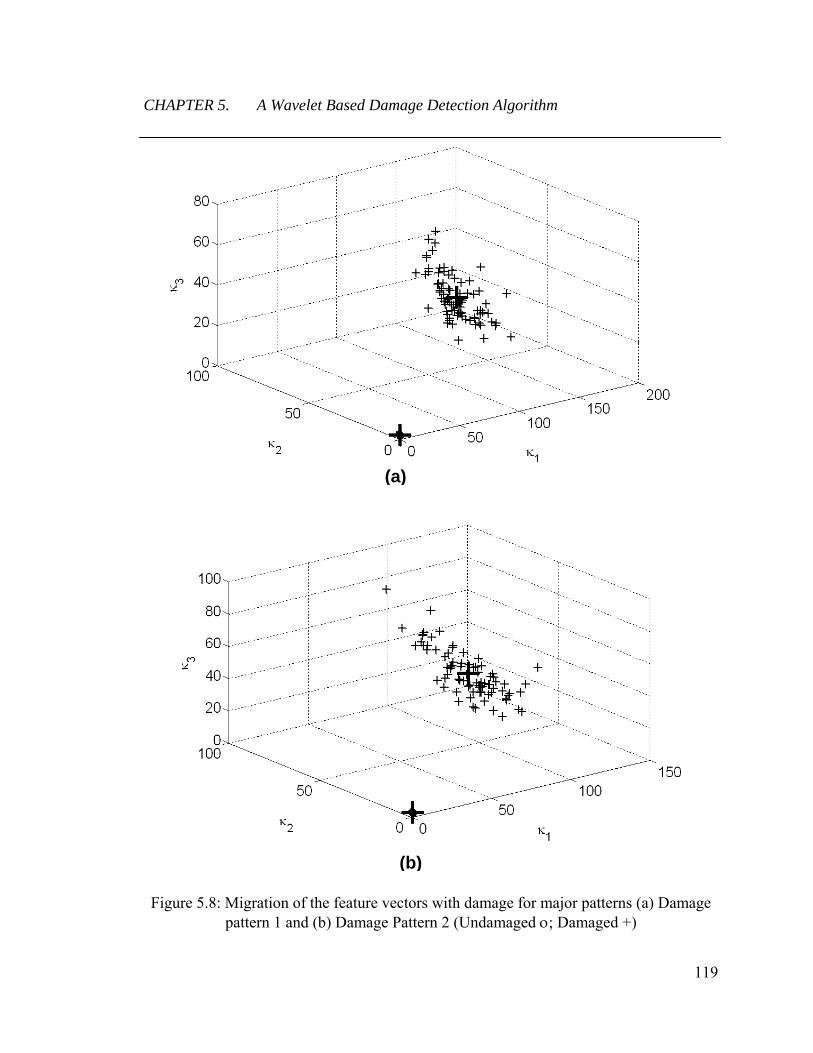
CHAPTER 5. A Wavelet Based Damage Detection Algorithm
119
(a)
(b)
Figure 5.8: Migration of the feature vectors with damage for major patterns (a) Damage pattern 1 and (b) Damage Pattern 2 (Undamaged ; Damaged +)

CHAPTER 5. A Wavelet Based Damage Detection Algorithm
120
5.3.2 Damage Extent Measure
The damage sensitive feature is defined as follows:
undamagednewT
undamagednewDM ,,,, ˆˆˆˆ μμμμ (5.7)
where, new,ˆ μ and undamaged,ˆ μ are the sample means of new and undamaged respectively.
Table 5.1 shows the variation of DM for all sensors and damage patterns as defined in the
ASCE Benchmark Experiment.
Table 5.1: Variation of DM for the DB4 wavelet based damage sensitive feature for all sensors and different damage patterns
Sensor DP1 DP2 DP3 DP4 DP5 DP6
1 98.07 100.35 11.20 72.14 72.14 NA 2 129.31 119.52 109.27 108.54 108.54 63.36 3 105.89 105.51 13.62 76.74 76.74 NA 4 144.37 127.67 123.77 123.16 123.16 71.53 5 91.81 96.54 14.31 71.37 71.37 NA 6 109.14 136.85 118.73 118.81 118.81 79.37 7 83.77 88.08 14.53 63.39 63.39 NA 8 106.05 128.91 105.65 105.22 105.22 71.21 9 102.21 99.38 19.18 68.82 68.82 NA
10 122.73 123.77 139.95 139.75 139.75 98.04 11 108.8023 103.50 22.41 72.94 72.94 NA 12 111.39 112.44 122.09 122.07 122.07 88.20 13 110.60 108.19 19.33 82.20 82.20 NA 14 123.01 108.23 126.89 126.21 126.21 83.69 15 98.18 97.01 17.89 71.56 71.56 NA 16 126.27 113.72 124.56 124.42 124.42 88.26
From Table 5.1, the following observations are made
The values of DM are correlated to the amount of damage. For damage
patterns 1 and 2, the values of DM are similar. A similar observation is made

CHAPTER 5. A Wavelet Based Damage Detection Algorithm
121
for damage patterns 3 and 4 for sensors placed on Faces 2 and 4 of the
structure (Figure 2.7).
For minor damage patterns 3 and 6, where the stiffness of brace is reduced on
Face 2 of the ASCE Benchmark Structure (Figure 2.7), the values of DM are
high for sensors on Faces 2 and 4 in comparison to Faces 1 and 3. It is also
observed that no damage is detected at sensors on Faces 1 and 3 for damage
pattern 6. These are denoted as NA in Table 5.1.
For sensors instrumented on Faces 1 and 3 of the ASCE Benchmark Structure
(Figure 2.7), the values of DM are significantly higher for damage pattern 4 in
comparison to damage pattern 3. For example, in the case of sensor 1, the
value of DM increases from 11.20 for DP 3 to 72.14 for DP 4. The reason for
this trend is because DP 3 involves the removal of a brace on Face 2, whereas
DP 4 is achieved by removing a brace on Face 1 and Face 2 of the structure.
All damage patterns are detected consistently using the wavelet based feature
vector.
For all damage patterns, the values of DM are higher for sensors on Faces 2
and 4. The reason for this behavior may be attributed to the fact that this is the
weak direction of the structure.
5.4 Summary
This chapter describes the development of a wavelet based damage detection algorithm.
The feature vector is based on the energies of wavelet coefficients, where the theoretical
formulation was developed in Chapter 4. This algorithm requires the creation of a
database of baseline measurements and computing the continuous Daubechies wavelet of
order four (DB4) wavelet coefficients at appropriate scales. Following this, principal

CHAPTER 5. A Wavelet Based Damage Detection Algorithm
122
components analyses are performed on the energies of the DB4 wavelet coefficients at
the first dyadic scale for comparing the new signal to the closest one in the database.
Once the optimal baseline signal in the database is chosen, feature vectors are calculated
using the energies of the DB4 wavelet coefficients at the fifth, sixth and seventh dyadic
scales. The k-means algorithm is used to obtain the means of the clusters and is used for
damage detection along with the gap statistic. A damage measure based on the Euclidean
distance between the means of the damaged and undamaged datasets is also described.
The k-means algorithm and Gap statistic works consistently well for detecting damage
patterns as defined for the ASCE Benchmark Structure. The values of DM also correlate
well with the extent of damage.
Although this algorithm show promise in identifying and quantifying damage, the
algorithm has to be validated using experimental and field data. These should be for
varying degrees of damage, loading conditions, environmental conditions such as
temperature and humidity, as well as different sequences of damage occurrences.
Different damage locations on the structure should be considered and damage sequences
should also be investigated. It is only after extensive experimentation and field testing
with calibration that these models can be widely applied. Never-the-less, the results
presented here are encouraging and represent a good initial step towards achieving this
goal.

123
Chapter 6
Summary, Conclusions and Future Work
Recent research efforts in wireless structural health monitoring have resulted in an
explosion in the development of new sensors. Little attention, however, has been focused
on the efficient and effective use of the data collected by these sensors. While these
wireless sensor networks enable dense instrumentation, the amount of data that needs to
be transmitted can prove to be prohibitive. The main difficulty arises from the low data
rates associated with low power ad-hoc wireless sensor networks. Thus, data transmission
over the wireless network is demanding, time consuming and can significantly reduce
power source life. Typically these data are required because current damage detection
algorithms perform global system level analysis rather than local sensor level analysis. In
this dissertation, three local sensor based damage diagnosis algorithms using statistical
signal processing and pattern classification techniques have been developed. The main
features of these algorithms are that they are simple, robust and computationally efficient.
The main contributions of this dissertation are as follows:
Demonstrated the use of statistical signal processing techniques to model the
vibration signal and extracting damage sensitive features for classification.

CHAPTER 6. Summary, Conclusions and Future Work
124
Derived closed form equations between the autoregressive and wavelet based
feature vectors and the physical characteristics of the structure. This provides a
quantitative insight into the working of these algorithms.
Used pattern classification schemes to discriminate features obtained from signals
of an undamaged structure and a damaged structure.
Derived damage metrics using the feature vectors to model damage extent.
6.1 Summary
The main premise in the algorithms developed is that the vibration signals are affected by
damage and these changes can be tracked to detect damage. Three damage detection
algorithms have been developed and are summarized in Table 6.1. In addition, a damage
extent measure has been formulated using an appropriate metric.
The first algorithm developed in Chapter 2 uses time series to model the vibration signal
and defines a damage sensitive feature DSF using the first three AR coefficients. A t-test
on the DSF’s is used to discriminate between an undamaged state and a damaged state.
This algorithm is valid for linear and stationary signals. The validation of the algorithm
with datasets obtained from the ASCE Benchmark Structure shows that all damage
patterns were identified. However, for minor damage patterns, it is noted that the
difference between the means of the damage sensitive features was lower in comparison
to that of major patterns.
The second algorithm, developed in Chapter 3, uses the first three AR coefficients as the
feature vector. Damage detection is performed using the Gaussian Mixture Models
(GMM’s) and the gap statistic. This algorithm is more robust than the algorithm 1 and is
again valid for linear, stationary signals. The damage measure has been developed using
the Mahalanobis distance between the means of the damaged and undamaged datasets.
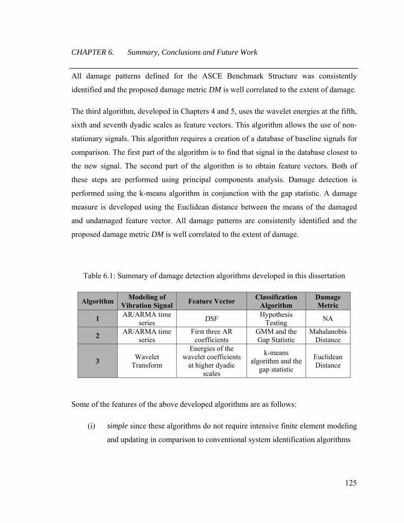
CHAPTER 6. Summary, Conclusions and Future Work
125
All damage patterns defined for the ASCE Benchmark Structure was consistently
identified and the proposed damage metric DM is well correlated to the extent of damage.
The third algorithm, developed in Chapters 4 and 5, uses the wavelet energies at the fifth,
sixth and seventh dyadic scales as feature vectors. This algorithm allows the use of non-
stationary signals. This algorithm requires a creation of a database of baseline signals for
comparison. The first part of the algorithm is to find that signal in the database closest to
the new signal. The second part of the algorithm is to obtain feature vectors. Both of
these steps are performed using principal components analysis. Damage detection is
performed using the k-means algorithm in conjunction with the gap statistic. A damage
measure is developed using the Euclidean distance between the means of the damaged
and undamaged feature vector. All damage patterns are consistently identified and the
proposed damage metric DM is well correlated to the extent of damage.
Table 6.1: Summary of damage detection algorithms developed in this dissertation
Algorithm Modeling of
Vibration Signal Feature Vector
Classification Algorithm
Damage Metric
1 AR/ARMA time
series DSF
Hypothesis Testing
NA
2 AR/ARMA time
series First three AR
coefficients GMM and the Gap Statistic
Mahalanobis Distance
3 Wavelet
Transform
Energies of the wavelet coefficients
at higher dyadic scales
k-means algorithm and the
gap statistic
Euclidean Distance
Some of the features of the above developed algorithms are as follows:
(i) simple since these algorithms do not require intensive finite element modeling
and updating in comparison to conventional system identification algorithms
CHAPTER 6. Summary, Conclusions and Future Work
126
(ii) robust since these algorithms are able to detect and quantify minor damage
patterns
(iii) computationally efficient since these algorithms use only processing of signals
at the sensor level and lead to significant saving in computation time.
6.2 Conclusions
The results of the application of the damage detection algorithm to vibration signals from
the ASCE Benchmark Structure lead to the following main conclusions:
All three algorithms are able to detect the existence of minor, moderate and severe
damage patterns in the ASCE Benchmark simulation experiment where minor,
moderate and severe damage corresponds to removal of single brace in a storey,
removal of a brace on two storeys and removal of all braces in two storeys,
respectively. It is also observed that the damage extent metric is well correlated to
the level of damage.
In Algorithm 1, it is shown that the AR model with 5-8 parameters is the optimal
time series for the vibration signals considered in the study. The differences in the
mean values of the damage sensitive feature DSF, as defined in Equation (2.6), is
higher for the major damage patterns in comparison to the minor damage patterns
and thus can be used as an indicator of damage extent. In the case of the minor
damage pattern (DP6), the confidence intervals of the difference in the means of
the DSF’s are not too high. Thus, a more sensitive feature / better classification
scheme is required for efficient damage detection.
Using Algorithm 2, it is seen that minor damage patterns are more consistently
identified using a more robust classification scheme. For all noise levels, major
and moderate damage patterns are detected since there is a large separation
CHAPTER 6. Summary, Conclusions and Future Work
127
between the damaged and undamaged feature vector clouds. However for large
noise levels, minor damage patterns, particularly damage pattern 6, do not appear
to be discriminated. The magnitude of the damage metric DM based on the
Mahalanobis distance appears to be highly correlated to the damage extent even
under the presence of noise. It is demonstrated that the magnitude of the DM
metric increases with increasing damage.
It is observed that the Haar wavelet is able to detect only major damage patterns.
In comparison, the Morlet wavelet performs much better and is able to detect
minor damage patterns. Thus for applications, it would be advisable to use
energies of the Morlet wavelet coefficients at higher scales. Algorithm 3 is more
sensitive to damage since the separation between the clouds of the Morlet wavelet
energies of the undamaged and damaged structure is much higher in comparison
to Algorithms 1 and 2.
6.3 Future Work and Research Needs
Although damage detection methodologies are getting more robust, no algorithm predicts
the location of damage accurately. Once damage diagnosis is complete, it is important to
perform damage prognosis. Almost no progress has been made in the field of damage
prognosis.
6.3.1 Damage Diagnosis
Damage detection is performed under various operational conditions, such as
environmental conditions such as temperature and humidity and loading conditions which
include the direction and magnitude of loading. Thus, algorithms are required to compare
feature vectors obtained from various loading conditions. Most of the currently developed

CHAPTER 6. Summary, Conclusions and Future Work
128
algorithms have not been tested on field data. Although field data are not readily
available, some of the currently available experimental data obtained are from a four
story steel frame used by the National Taiwan University (Lynch et al., 2006) and field
data obtained from a bridge in Switzerland (Wenzel, 2006). To gain wide adoption,
damage detection algorithms need to be tested with field data.
Damage localization is still an open problem in structural health monitoring. The damage
extent metric (DM) developed in this dissertation does not show any spatial pattern
(Figure 2.9). Thus, damage localization could not be achieved. One of the main reasons
for this is because acceleration measurements are global in nature and thus cannot capture
local effects. Thus, using strain data, which is a local measurement, could help in
localization of damage (Noh et al., 2007). Measurement data near cracks is also lacking
and simple experiments need to be generated on small samples simulating the initiation
and propagation of cracks. Measurements (vibration and strain) need to be obtained at
various stages of the crack propagation and at different distances from the crack. Such
measurements will also aid in the localization of the damage.
Furthermore, more research needs to be carried out in the field of data fusion, where
information from various sensors is statistically combined to obtain a more robust
decision (Wald, 1998). In addition, it would be ideal to fuse results from model based
methodologies (using physical models) and non model based algorithms (as presented in
this dissertation) to obtain more robust and meaningful results.
6.3.2 Damage Prognosis
The area of damage prognosis is still in its infancy. Damage prognosis deals with the
calculation of residual strength of the structure and the prediction of the residual life
capacity of the structure (Rytter, 1993). To this end, algorithms for local and global
damage prognosis have to be developed. These algorithms would involve the use of
modeling and simulation. These include physics based models, surrogate models, coupled

CHAPTER 6. Summary, Conclusions and Future Work
129
models and knowledge-based models (Farrar et al., 2003). Physics based models
generally involve finite element modeling where the model has to be updated at each
stage of progressive damage. These models are computationally very expensive and thus
require surrogate models to reduce the computational complexity of the problem.
Surrogate models generally include machine learning algorithms such as neural networks,
self organizing maps etc. Also calibration and validation of these models are required.
Uncertainty quantification becomes an important issue in these models. Modeling,
loading and measurement uncertainties have to be evaluated. For prediction of the
residual life of the structure, time variant reliability based methods can be used. The
challenges of these tasks are explained by Farrar et al., 2003.

130
Bibliography
J. A. Bilmes. A Gentle Tutorial of the EM Algorithm and its Application to Parameter
Estimation for Gaussian Mixture and Hidden Markov Models, Technical Report 97-021,
International Computer Science Institute, University of California. Berkeley, 1998.
R. N. Bracewell. The Fourier Transform and its Applications, McGraw Hill, Third
Edition, New York, 1999.
P. J. Brockwell and R. A. Davis. Introduction to Time Series and Forecasting, Springer-
Verlag, Second Edition, New York, 2002.
F- K. Chang. Proceedings of the 1st, 2nd and 3rd International Workshops on Structural
Health Monitoring, Stanford University, Stanford, CA. CRC Press, New York, 1999,
2001, 2003 and 2005.
S. W. Doebling, C. R. Farrar, M. B. Prime and D. W. Shevitz. Damage Identification and
Health Monitoring of Structural and Mechanical Systems from Changes in Their
Vibration Characteristics: A Literature Review, Los Alamos National Laboratory Report
LA-13070-MS, Los Alamos National Laboratory, Los Alamos, NM, 1996.
R. O. Duda, P. E. Hart and D. G. Stork. Pattern Classification, Wiley-Interscience
Publications, New York, 2001.
C. R. Farrar and T. A. Duffey. “Vibration based Damage Detection in Rotating
Machinery and Comparison to Civil Engineering Applications,” Proceedings of Damage
Assessment of Structures, Dublin, Ireland, 1999.

Bibliography
131
C. R. Farrar, H. Sohn, F. M. Hemez, M. C. Anderson, M. T. Bement, P. J. Cornwell, S.
W. Doebling, J. F. Schultze, N. Lieven and A. N. Robertson. Damage Prognosis: Current
Status and Future Needs, Los Alamos National Laboratory Report LA-14501-MS, Los
Alamos National Laboratory, Los Alamos, NM, 2003
R. Fox and M. Kapoor. “Rate of Change of Eigenvalues and Eigenvectors,” AIAA
Journal 6:2426-2429, 1968.
R. Ghanem and F. Romeo. “A Wavelet Based Approach for Identification of Linear Time
Varying Dynamical Systems,” Journal of Sound and Vibration, 234(5): 555-576.
T. Hastie, R. Tibshirani and J. Freidman. Elements of Statistical Learning: Data Mining,
Inference and Prediction, Springer Verlag, First edition, New York, 2001.
Z. K. Hou, M. Noori and R. St. Amand. “Wavelet-based Approach for Structural Damage
Detection,” ASCE Journal of Engineering Mechanics, 126(7): 677-683, 2000.
E. A. Johnson, H. F. Lam, L. S. Katafygiotis and J. L. Beck. “A Benchmark Problem for
Structural Health Monitoring and Damage Detection,” Proceedings of 14th Engineering
Mechanics Conference, Austin, TX, USA, 2000.
E. A. Johnson, H. F. Lam, L. S. Katafygiotis and J. L. Beck. “Phase I IASC-ASCE
Structural Health Monitoring Benchmark Problem Using Simulated Data,” Journal of
Engineering Mechanics, 130(1):3-15, 2004.
T. Kijewski and A. Kareem. “Wavelet Transforms for System Identification:
Considerations for Civil Engineering Applications,” Journal of Computer-Aided Civil
and Infrastructure Engineering, 18: 341-357, 2003.
E. Kreyzig. Advanced Engineering Mathematics, John Wiley and Sons, Eighth Edition,
New York, 1998.

Bibliography
132
J. P. Lynch. “Linear Classification of System Poles for Structural Damage Detection
Using Piezoelectric Active Sensors,” Proceedings of SPIE 11th Annual International
Symposium on Smart Structures and Materials, San Diego, CA, USA, 2004.
J. P. Lynch, Y. Wang, K-C. Lu, T-C. Hou and C-H. Loh. “Post-Seismic Damage
Assessment of Steel Structures Instrumented with Self-Interrogating Wireless Sensors,”
Proceedings of the 8th National Conference on Earthquake Engineering (8NCEE), San
Francisco, CA, 2006.
J. P. Lynch, A. Sundararajan, K. H. Law and A. S. Kiremidjian. “Embedding Algorithms
in a Wireless Structural Monitoring System,” Proceedings of the International
Conference on Advances and New Challenges in Earthquake Engineering Research
(ICANCEER02), Hong Kong, China, 2002.
J. P. Lynch, A. Sundararajan, K. H. Law, A. S. Kiremidjian and E. Carryer. “Embedding
Damage Detection Algorithms in a Wireless Sensing Unit for Attainment of Operational
Power Efficiency,” Smart Materials and Structures, 13(4):800-810, 2004.
N. M. M Maia and J. M. M Silva. Theoretical and Experimental Modal Analysis,
Research Studies Press, Hertfordshire, England, 1998.
S. Mallat. A Wavelet Tour of Signal Processing, Academic Press, New York, 1999.
K. V. Mardia, J. T Kent and J. M. Bibby. Multivariate Analysis, Academic Press,
London, 2003.
K. K. Nair and A. S. Kiremidjian. “Time Series Based Structural Damage Detection
Algorithm Using Gaussian Mixtures Modeling,” ASME Journal of Dynamic Systems,
Measurement and Control, 129(3): 285-293, 2007.
K. K. Nair, A. S. Kiremidjian and K. H. Law. “Time Series Based Damage Detection and
Localization Algorithm with Application to the ASCE benchmark Structure,” Journal of
Sound and Vibration, 291 (2): 349-368, 2006.

Bibliography
133
R. B. Nelson. “Simplified Calculations of Eigenvector Derivatives for Large Dynamic
Systems,” AIAA Journal, 14: 1201-1205, 1976.
H. Noh, K. K. Nair, A. S. Kiremidjian and C-H. Loh. “Application of a Time Series
Based Damage Detection Algorithm to the Taiwanese Benchmark Experiment,”
Proceedings of the 10th International Conference on Application of Statistics and
Probability in Civil Engineering (ICASP10), University of Tokyo, Tokyo, 2007.
A. V. Oppenheim and R. W. Schafer. Digital Signal Processing, First Edition, Pearson
Higher Education, 1986.
J. A. Rice. Mathematical Statistics and Data Analysis, Second Edition, Duxbury Press,
Second Edition, 1999.
A. Rytter. Vibrational Based Inspection of Civil Engineering Structures, PhD
Dissertation, Department of Building Technology and Structure Engineering, Aalborg
University, Denmark, 1993.
H. Sohn, M. Dzwonczyk, E. G. Straser, A. S. Kiremidjian, K. H. Law and T. Meng. “An
Experimental Study of Temperature Effect on Modal Parameters of the Alamosa Canyon
Bridge,” Earthquake Engineering and Structural Dynamics, John Wiley & Sons, 28(9):
879-897, 1999.
H. Sohn and C. R. Farrar. “Damage Diagnosis Using Time Series Analysis of Vibration
Signals,” Smart Materials and Structures, 10(3): 446-451, 2001.
H. Sohn, C. R. Farrar, H. F. Hunter and K. Worden. Applying the LANL Statistical
Pattern Recognition Paradigm for Structural Health Monitoring to Data from a Surface-
Effect Fast Patrol Boat, Los Alamos National Laboratory Report LA-13761-MS, Los
Alamos National Laboratory, Los Alamos, NM, 2001.

Bibliography
134
W. J. Staszewski. “Identification of Non-Linear Systems Using Multi-Scale Ridges and
Skeletons of the Wavelet Transform,” Journal of Sound and Vibration, 214(4): 639-658,
2000.
E. G. Straser and A. S. Kiremidjian. Modular Wireless Damage Monitoring System for
Structures, Technical Report No. 128, John A. Blume Earthquake Engineering Center,
Department of Civil and Environmental Engineering, Stanford University, Stanford, CA,
1998.
Z. Sun, and C. C. Chang. “Statistical Wavelet Based Method for Structural Health
Monitoring,” ASCE Journal of Structural Engineering, 130(7): 1055-1062, 2004.
R. Tibshirani, G. Walther and T. Hastie. “Estimating the Number of Clusters in a Dataset
via the Gap Statistic,” Journal of the Royal Statistical Society: Series B, 63(2): 411-423,
2001.
The ASCE Benchmark Group Webpage, http:// wusceel.cive.wustl.edu/ asce.shm/
benchmarks.htm, 2000.
L. Wald. “Data Fusion: A Conceptual Approach for an Efficient Exploitation of Remote
Sensing Images,” Proceedings of EARSeL Conference on Fusion of Earth Data, 17-23,
1998.
H. Wenzel, Personal Communication, 2006.