damage models and algorithms for assessment of structures under operating conditions
TRANSCRIPT

Damage Models and Algorithmsfor Assessment of Structuresunder Operating Conditions
© 2009 Taylor & Francis Group, London, UK
Structures and Infrastructures Series
ISSN 1747-7735
Book Series Editor:
Dan M. FrangopolProfessor of Civil Engineering andFazlur R. Khan Endowed Chair of Structural Engineering and ArchitectureDepartment of Civil and Environmental EngineeringCenter for Advanced Technology for Large Structural Systems (ATLSS Center)Lehigh UniversityBethlehem, PA, USA
Volume 5
© 2009 Taylor & Francis Group, London, UK
Damage Models andAlgorithmsforAssessment of Structuresunder Operating Conditions
Siu-Seong Law1 and Xin-Qun Zhu2
1Civil and Structural Engineering Department, Hong Kong PolytechnicUniversity, Kowloon, Hong Kong2School of Engineering, University of Western Sydney, Australia
© 2009 Taylor & Francis Group, London, UK
Colophon
Book Series Editor :Dan M. Frangopol
Volume Authors:Siu-Seong Law & Xin-Qun Zhu
Cover illustration:Spatial mathematical model of the Tsing Ma Suspension Bridge Deck.
Taylor & Francis is an imprint of the Taylor & Francis Group,an informa business
© 2009 Taylor & Francis Group, London, UK
Typeset by Charon Tec Ltd (A Macmillan company), Chennai, IndiaPrinted and bound in Great Britain by Antony Rowe (a CPI Group company),Chippenham, Wiltshire
All rights reserved. No part of this publication or the informationcontained herein may be reproduced, stored in a retrieval system,or transmitted in any form or by any means, electronic, mechanical,by photocopying, recording or otherwise, without written priorpermission from the publishers.
Although all care is taken to ensure integrity and the quality of thispublication and the information herein, no responsibility isassumed by the publishers nor the author for any damage to theproperty or persons as a result of operation or use of thispublication and/or the information contained herein.
British Library Cataloguing in Publication DataA catalogue record for this book is available from the British Library
Library of Congress Cataloging-in-Publication Data
Law, S. S.Damage models and algorithms for assessment of structures under
operating conditions / S.S. Law and X.Q. Zhu.p. cm. — (Structures and infrastructures series, ISSN 1747-7735 ; v. 5)
Includes bibliographical references.ISBN 978-0-415-42195-9 (hardcover : alk. paper) — ISBN 978-0-203-87087-7
(e-book : alk. paper) 1. Structural failures—Mathematical models. 2. Buildings—Evaluation—Mathematics. I. Zhu, X. Q. II. Title. III. Series.TA656.L39 2009624.1′71015118—dc22
2009017893
Published by: CRC Press/BalkemaP.O. Box 447, 2300 AK Leiden,The Netherlandse-mail: [email protected] – www.taylorandfrancis.co.uk – www.balkema.nl
ISBN13 978-0-415-42195-9(Hbk)ISBN13 978-0-203-87087-7(eBook)Structures and Infrastructures Series: ISSN 1747-7735Volume 5
© 2009 Taylor & Francis Group, London, UK

Table of Contents
Editorial XIIIAbout the Book Series Editor XVPreface XVIIDedication XXIAcknowledgements XXIIIAbout the Authors XXV
Chapter 1 Introduction 1
1.1 Condition monitoring of civil infrastructures 11.1.1 Background to the book 11.1.2 What information should be obtained from the structural health
monitoring system? 11.2 General requirements of a structural condition assessment algorithm 31.3 Special requirements for concrete structures 31.4 Other considerations 4
1.4.1 Sensor requirements 41.4.2 The problem of a structure with a large number of
degrees-of-freedom 41.4.3 Dynamic approach versus static approach 51.4.4 Time-domain approach versus frequency-domain approach 51.4.5 The operation loading and the environmental effects 51.4.6 The uncertainties 6
1.5 The ideal algorithm/strategy of condition assessment 6
Chapter 2 Mathematical concepts for discrete inverse problems 9
2.1 Introduction 92.2 Discrete inverse problems 9
2.2.1 Mathematical concepts 92.2.2 The ill-posedness of the inverse problem 10
© 2009 Taylor & Francis Group, London, UK
VI Tab le o f Contents
2.3 General inversion by singular value decomposition 112.3.1 Singular value decomposition 112.3.2 The generalized singular value decomposition 122.3.3 The discrete Picard condition and filter factors 13
2.4 Solution by optimization 152.4.1 Gradient-based approach 152.4.2 Genetic algorithm 172.4.3 Simulated annealing 19
2.5 Tikhonov regularization 192.5.1 Truncated singular value decomposition 202.5.2 Generalized cross-validation 212.5.3 The L-curve 23
2.6 General optimization procedure for the inverse problem 252.7 The criteria of convergence 252.8 Summary 25
Chapter 3 Damage description and modelling 27
3.1 Introduction 273.1.1 Damage models 273.1.2 Model on pre-stress 27
3.2 Damage-detection-oriented model 283.2.1 Beam element with end flexibilities 28
3.2.1.1 Hybrid beam with shear flexibility 293.2.1.2 Hybrid beam with both shear and flexural
flexibilities 423.2.2 Decomposition of system matrices 46
3.2.2.1 The generic element 473.2.2.2 The eigen-decomposition 52
3.2.3 Super-element 693.2.3.1 Beam element with semi-rigid joints 703.2.3.2 The Tsing Ma bridge deck 73
3.2.4 Concrete beam with flexural crack and debonding at the steeland concrete interface 78
3.2.5 Beam with unbonded pre-stress tendon 863.2.6 Pre-stressed concrete box-girder with bonded tendon 923.2.7 Models with thin plate 97
3.2.7.1 Anisotropic model of elliptical crack with strainenergy equivalence 97
3.2.7.2 Thin plates with anisotropic crack from dynamiccharacteristic equivalence 100
3.2.8 Model with thick plate 1073.2.8.1 Thick plate with anisotropic crack model 107
3.2.9 Model of thick plate reinforced with Fibre-Reinforced-Plastic 1133.2.9.1 Damage-detection-oriented model of delamination
of fibre-reinforced plastic and thick plate 1163.3 Conclusions 128
© 2009 Taylor & Francis Group, London, UK
Tab le o f Contents VII
Chapter 4 Model reduction 131
4.1 Introduction 1314.2 Static condensation 1314.3 Dynamic condensation 1324.4 Iterative condensation 1354.5 Moving force identification using the improved reduced system 135
4.5.1 Theory of moving force identification 1354.5.2 Numerical example 137
4.6 Structural damage detection using incomplete modal data 1394.6.1 Mode shape expansion 1394.6.2 Application 140
4.7 Remarks on more recent developments 144
Chapter 5 Damage detection from static measurement 145
5.1 Introduction 1455.2 Constrained minimization 145
5.2.1 Output error function 1465.2.1.1 Displacement output error function 1465.2.1.2 Strain output error function 147
5.2.2 Damage detection from the static response changes 1485.2.3 Damage detection from combined static and dynamic
measurements 1505.3 Variation of static deflection profile with damage 152
5.3.1 The static deflection profile 1525.3.2 Spatial wavelet transform 154
5.4 Application 1545.4.1 Damage assessment of concrete beams 154
5.4.1.1 Effect of measurement noise 1545.4.1.2 Damage identification 1565.4.1.3 Damage evolution under load 1585.4.1.4 Damage identification – Simulating practical
assessment 1595.4.2 Assessment of bonding condition in reinforced concrete beams 160
5.4.2.1 Local beam damage identification 1605.4.2.2 Identification of local bonding 1615.4.2.3 Simultaneous identification of local bonding and
beam damages 1635.5 Limitations with static measurements 1645.6 Conclusions 165
Chapter 6 Damage detection in the frequency domain 167
6.1 Introduction 1676.2 Spatial distributed system 167
© 2009 Taylor & Francis Group, London, UK
VIII Tab le o f Contents
6.3 The eigenvalue problem 1686.3.1 Sensitivity of eigenvalues and eigenvectors 1686.3.2 System with close or repeated eigenvalues 170
6.4 Localization and quantification of damage 1726.5 Finite element model updating 1726.6 Higher order modal parameters and their sensitivity 173
6.6.1 Elemental modal strain energy 1736.6.1.1 Model strain energy change sensitivity 174
6.6.2 Modal flexibility 1766.6.2.1 Model flexibility sensitivity 177
6.6.3 Unit load surface 1806.7 The curvatures 180
6.7.1 Mode shape curvature 1816.7.2 Modal flexibility curvature 1816.7.3 Unit load surface curvature 1816.7.4 Chebyshev polynomial approximation 1826.7.5 The gap-smoothing technique 184
6.7.5.1 The uniform load surface curvature sensitivity 1856.7.6 Numerical examples of damage localization 188
6.7.6.1 Simply supported plate 1896.7.6.2 Study on truncation effect 1896.7.6.3 Comparison of curvature methods 1916.7.6.4 Resolution of damage localization 1926.7.6.5 Cantilever plate 1926.7.6.6 Effect of sensor sparsity 1926.7.6.7 Effect of measurement noise 1956.7.6.8 When the damage changes the boundary condition
of the structure 1966.8 Conclusions 197
Chapter 7 System identification based on response sensitivity 199
7.1 Time-domain methods 1997.2 The response sensitivity 199
7.2.1 The computational approach 1997.2.2 The analytical formulation 2007.2.3 Main features of the response sensitivity 201
7.3 Applications in system identification 2057.3.1 Excitation force identification 205
7.3.1.1 The response sensitivity 2077.3.1.2 Experimental verification 207
7.3.2 Condition assessment from output only 2097.3.2.1 Algorithm of iteration 2097.3.2.2 Experimental verification 211
7.3.3 Removal of the temperature effect 2127.3.4 Identification with coupled system parameters 2157.3.5 Condition assessment of structural parameters having
a wide range of sensitivities 216
© 2009 Taylor & Francis Group, London, UK
Tab le o f Contents IX
7.4 Condition assessment of load resistance of isotropic structuralcomponents 216
7.4.1 Dynamic test for model updating 2187.4.2 Damage scenarios 2197.4.3 Dynamic test for damage detection 219
Damage scenario E1 219Damage scenario E2 221Damage scenario E3 221The false positives in the identified results 222
7.5 System identification under operational loads 2237.5.1 Existing approaches 223
7.5.1.1 The equation of motion 2237.5.1.2 Damage detection from displacement measurement 224
7.5.2 The generalized orthogonal function expansion 2267.5.3 Application to a bridge-vehicle system 227
7.5.3.1 The vehicle and bridge system 2277.5.3.2 The residual pre-stress identification 229
7.6 Conclusions 230
Chapter 8 System identification with wavelet 231
8.1 Introduction 2318.1.1 The wavelets 2318.1.2 The wavelet packets 233
8.2 Identification of crack in beam under operating load 2358.2.1 Dynamic behaviour of the cracked beam subject to moving load 2368.2.2 The crack model 2378.2.3 Crack identification using continuous wavelet transform 2398.2.4 Numerical study 2408.2.5 Experimental verification 243
8.3 The sensitivity approach 2458.3.1 The wavelet packet component energy sensitivity and the
solution algorithm 246The solution algorithm 247
8.3.2 The wavelet sensitivity and the solution algorithm 247Analytical approach 248Computational approach 249The solution algorithm 250
8.3.3 The wavelet packet transform sensitivity 2518.3.4 Damage information from different wavelet bandwidths 252
Damage scenarios and their detection 255Effect of measurement noise and model error 256
8.3.5 Damage information from different wavelet coefficients 2578.3.6 Frequency and energy content of wavelet coefficients 258
Comparison with response sensitivity 258Damage identification 259Effect of model error 260
8.3.7 Noise effect 263
© 2009 Taylor & Francis Group, London, UK
X Tab le o f Contents
8.4 Approaches that are independent of input excitation 2648.4.1 The unit impulse response function sensitivity 264
8.4.1.1 Wavelet-based unit impulse response 2658.4.1.2 Impulse response function via discrete wavelet
transform 2678.4.1.3 Solution algorithm 2688.4.1.4 Simulation study 269
Damage identification with model error andnoise effect 269
8.4.1.5 Discussions 2708.4.2 The covariance sensitivity 271
8.4.2.1 Covariance of measured responses 2718.4.2.2 When under single random excitation 2728.4.2.3 When under multiple random excitations 2738.4.2.4 Sensitivity of the cross-correlation function 275
8.5 Condition assessment including the load environment 2758.5.1 Sources of external excitation 2758.5.2 Under earthquake loading or ground-borne excitation 275
8.5.2.1 Simulation studies 2758.5.2.2 The sensitivities 2768.5.2.3 Damage identification from WPT sensitivity and
response sensitivity 277Effect of model error and noise 279Performance from a subset of the measured response 280
8.5.3 Under normal random support excitation 2808.5.3.1 Damage localization based on mode shape changes 2818.5.3.2 Laboratory experiment 282
Modelling of the structure 282Ambient vibration test for damage detection 283Damage scenarios 284Model improvement for damage detection 285
8.6 Conclusions 286
Chapter 9 Uncertainty analysis 287
9.1 Introduction 2879.2 System uncertainties 288
9.2.1 Modelling uncertainty 2889.2.2 Parameter uncertainty 2899.2.3 Measurement and environmental uncertainty 289
9.3 System identification with parameter uncertainty 2909.3.1 Monte Carlo simulation 2919.3.2 Integrated perturbed and Bayesian method 291
9.4 Modelling the uncertainty 2949.5 Propagation of uncertainties in the condition assessment process 295
9.5.1 Theoretical formulation 2959.5.1.1 Uncertainties of the system 295
© 2009 Taylor & Francis Group, London, UK

Tab le o f Contents XI
9.5.1.2 Derivatives of local damage with respect to theuncertainties 296
9.5.1.3 Uncertainty in the system parameter 2969.5.1.4 Uncertainty in the exciting force 2979.5.1.5 Uncertainty in the structural response 2989.5.1.6 Statistical characteristics of the damage vector 2999.5.1.7 Statistical analysis in damage identification 301
9.5.2 Numerical example 3019.5.2.1 The structure 3019.5.2.2 Uncertainty with the mass density 3029.5.2.3 Uncertainty with the elastic modulus of material 3049.5.2.4 Uncertainty with the excitation force and measured
response 3059.5.3 Discussions 306
9.6 Integration of system uncertainties with the reliability analysis ofa box-section bridge deck structure 3069.6.1 Numerical example 3079.6.2 Condition assessment 3089.6.3 Reliability analysis 310
9.7 Conclusions 313
References 315Subject Index 329Structures and Infrastructures Series 333
© 2009 Taylor & Francis Group, London, UK

Editorial
Welcome to the Book Series Structures and Infrastructures.Our knowledge to model, analyze, design, maintain, manage and predict the life-
cycle performance of structures and infrastructures is continually growing. However,the complexity of these systems continues to increase and an integrated approachis necessary to understand the effect of technological, environmental, economical,social and political interactions on the life-cycle performance of engineering structuresand infrastructures. In order to accomplish this, methods have to be developed tosystematically analyze structure and infrastructure systems, and models have to beformulated for evaluating and comparing the risks and benefits associated with variousalternatives. We must maximize the life-cycle benefits of these systems to serve the needsof our society by selecting the best balance of the safety, economy and sustainabilityrequirements despite imperfect information and knowledge.
In recognition of the need for such methods and models, the aim of this Book Seriesis to present research, developments, and applications written by experts on the mostadvanced technologies for analyzing, predicting and optimizing the performance ofstructures and infrastructures such as buildings, bridges, dams, underground con-struction, offshore platforms, pipelines, naval vessels, ocean structures, nuclear powerplants, and also airplanes, aerospace and automotive structures.
The scope of this Book Series covers the entire spectrum of structures and infrastruc-tures. Thus it includes, but is not restricted to, mathematical modeling, computer andexperimental methods, practical applications in the areas of assessment and evalua-tion, construction and design for durability, decision making, deterioration modelingand aging, failure analysis, field testing, structural health monitoring, financial plan-ning, inspection and diagnostics, life-cycle analysis and prediction, loads, maintenancestrategies, management systems, nondestructive testing, optimization of maintenanceand management, specifications and codes, structural safety and reliability, systemanalysis, time-dependent performance, rehabilitation, repair, replacement, reliabilityand risk management, service life prediction, strengthening and whole life costing.
This Book Series is intended for an audience of researchers, practitioners, andstudents world-wide with a background in civil, aerospace, mechanical, marine andautomotive engineering, as well as people working in infrastructure maintenance,monitoring, management and cost analysis of structures and infrastructures. Some vol-umes are monographs defining the current state of the art and/or practice in the field,and some are textbooks to be used in undergraduate (mostly seniors), graduate and
© 2009 Taylor & Francis Group, London, UK

XIV Ed i tor ia l
postgraduate courses. This Book Series is affiliated to Structure and InfrastructureEngineering (http://www.informaworld.com/sie), an international peer-reviewed jour-nal which is included in the Science Citation Index.
It is now up to you, authors, editors, and readers, to make Structures andInfrastructures a success.
Dan M. FrangopolBook Series Editor
© 2009 Taylor & Francis Group, London, UK
About the Book Series Editor
Dr. Dan M. Frangopol is the first holder of the FazlurR. Khan Endowed Chair of Structural Engineering andArchitecture at Lehigh University, Bethlehem, Pennsylvania,USA, and a Professor in the Department of Civil andEnvironmental Engineering at Lehigh University. He is alsoan Emeritus Professor of Civil Engineering at the Universityof Colorado at Boulder, USA, where he taught for more thantwo decades (1983–2006). Before joining the University ofColorado, he worked for four years (1979–1983) in struc-tural design with A. Lipski Consulting Engineers in Brussels,Belgium. In 1976, he received his doctorate in Applied Sci-
ences from the University of Liège, Belgium, and holds two honorary doctorates(Doctor Honoris Causa) from the Technical University of Civil Engineering inBucharest, Romania, and the University of Liège, Belgium. He is a Fellow of theAmerican Society of Civil Engineers (ASCE), American Concrete Institute (ACI), andInternational Association for Bridge and Structural Engineering (IABSE). He is alsoan Honorary Member of both the Romanian Academy of Technical Sciences and thePortuguese Association for Bridge Maintenance and Safety. He is the initiator andorganizer of the Fazlur R. Khan Lecture Series (www.lehigh.edu/frkseries) at LehighUniversity.
Dan Frangopol is an experienced researcher and consultant to industry and govern-ment agencies, both nationally and abroad. His main areas of expertise are structuralreliability, structural optimization, bridge engineering, and life-cycle analysis, design,maintenance, monitoring, and management of structures and infrastructures. He isthe Founding President of the International Association for Bridge Maintenance andSafety (IABMAS, www.iabmas.org) and of the International Association for Life-CycleCivil Engineering (IALCCE, www.ialcce.org), and Past Director of the Consortium onAdvanced Life-Cycle Engineering for Sustainable Civil Environments (COALESCE).He is also the Chair of the Executive Board of the International Association forStructural Safety and Reliability (IASSAR, www.columbia.edu/cu/civileng/iassar) andthe Vice-President of the International Society for Health Monitoring of IntelligentInfrastructures (ISHMII, www.ishmii.org). Dan Frangopol is the recipient of severalprestigious awards including the 2008 IALCCE Senior Award, the 2007 ASCE ErnestHoward Award, the 2006 IABSE OPAC Award, the 2006 Elsevier Munro Prize, the2006 T. Y. Lin Medal, the 2005 ASCE Nathan M. Newmark Medal, the 2004 Kajima
© 2009 Taylor & Francis Group, London, UK

XVI About the Book Ser ies Ed i tor
Research Award, the 2003 ASCE Moisseiff Award, the 2002 JSPS Fellowship Awardfor Research in Japan, the 2001 ASCE J. James R. Croes Medal, the 2001 IASSARResearch Prize, the 1998 and 2004 ASCE State-of-the-Art of Civil Engineering Award,and the 1996 Distinguished Probabilistic Methods Educator Award of the Society ofAutomotive Engineers (SAE).
Dan Frangopol is the Founding Editor-in-Chief of Structure and InfrastructureEngineering (Taylor & Francis, www.informaworld.com/sie) an international peer-reviewed journal, which is included in the Science Citation Index. This journal isdedicated to recent advances in maintenance, management, and life-cycle performanceof a wide range of structures and infrastructures. He is the author or co-author of over400 refereed publications, and co-author, editor or co-editor of more than 20 bookspublished by ASCE, Balkema, CIMNE, CRC Press, Elsevier, McGraw-Hill, Taylor &Francis, and Thomas Telford and an editorial board member of several internationaljournals. Additionally, he has chaired and organized several national and internationalstructural engineering conferences and workshops. Dan Frangopol has supervised over70 Ph.D. and M.Sc. students. Many of his former students are professors at majoruniversities in the United States, Asia, Europe, and South America, and several areprominent in professional practice and research laboratories.
For additional information on Dan M. Frangopol’s activities, please visitwww.lehigh.edu/∼dmf206/
© 2009 Taylor & Francis Group, London, UK
Preface
The economy of the world has undergone a significant leap in the last few decades.Many major infrastructures were constructed to meet the growing demand of rapidand heavy inter-city passages and freight transportation. These structures are impor-tant to the economy, and significant losses will be incurred if they are out of service.Some sort of health monitoring system has been included in some of these infrastruc-tures as part of the management system to ensure the smooth operation of these civilstructures. Operational data has been collected over many years and yet there is noanalysis algorithm which can give the exact working state of the structure on-line. Themaintenance engineer would like to know the exact location and damage state of thestructural components involved in a damage scenario after an earthquake, a majorintentional attack or an unintentional accident to the structure. This knowledge isrequired in a matter of hours for life saving or any necessary military action. Also, theclient would like to have a rapid diagnosis of the structure to make a decision on anynecessary remedial work.
Existing methods that use the modal parameters for a diagnosis of the structure arenot feasible, as they demand a large number of measurement stations and full or partialclosure of the structure. Also, measurement with operation loads on top would notgive an accurate estimate of the modal parameters. Other existing methods that usetime-response histories do not include the operating load in the analysis. This book isdevoted to the condition assessment problem with the structure under operating loads,with many illustrations related to a bridge deck under a group of moving vehicularloads. The loading environment under which the structure is exposed serves as theexcitation. It may be a group of vehicular loads, earthquake excitation or ambientrandom excitation at the supports. It may be the wind loads acting at the deck level ina flexible cable-supported bridge deck. Different algorithms based on these excitationsare discussed. These excitation forces are used directly in the equation of motion of thestructure for the estimation of local changes in the structure, and different time-domainapproaches, including those developed by the authors, are discussed in detail.
These algorithms enable real-time identification with deterministic results on thestate of the structure. This meets the needs of maintenance engineers, who wouldlike to know the damage state of the structural components, so that they can judgethe suitability of remedial measures and estimate the effect on the performance ofthe structure. This also matches the current practice of deterministic design of the
© 2009 Taylor & Francis Group, London, UK
XVIII Pre face
infrastructure, thus giving the maintenance engineer a good feeling about the safety ofthe structure.
A description of the type of damage is an essential component of structural conditionassessment. However, damage models are scare and are mostly limited to crack(s) in abeam. This book covers a group of Damage-Detection-Oriented Models, including anew decomposition of the elemental matrices of the beam element and plate elementthat automatically differentiates changes in the different load resisting stiffnesses ofthe structural component. These models give a more precise description of the dam-age component than ordinary models, which usually treat the damage as an averagereduction in the elastic modulus of the material, and hence they are more suitable fordetecting damage.
The owner of the infrastructure is also concerned with the safety and reliability ofthe structure in the form of a statistical estimate of its remaining life. A method thatcan extend the deterministic condition assessment to provide statistical information isalso included in this book.
The group of methods and algorithms described in this book can be implemented foron-line condition assessment of a structure through model updating during the courseof an earthquake, when under normal ambient excitation or operation excitation frompassing vehicles. These capabilities are demonstrated with examples of the conditionassessment of different structures supplemented with major references.
Chapter 1 gives the background to structural condition assessment and its main com-ponents. The requirements of an ideal and practical structural condition assessmentalgorithm are discussed. Chapter 2 gives a summary of the mathematical techniquesthat are needed to solve the inverse problem with the condition assessment algorithmspresented in this book. The Tikhonov regularization and other optimization methodsare noted to be frequently used with the algorithms.
Chapter 3 summarizes the more recently developed models on damage in frameand plate elements. These include, the crack size and orientation in a thin and thickplate; the delamination of Fibre Reinforced Plastic from a concrete plate; the super-element model of the Tsing Ma Bridge deck; a general-purpose joint model with bothrotational and transverse flexibility; and the pre-stressing effect of a concrete member.The stiffness matrix of a rectangular shell element can be decomposed analytically intoits macro-stiffnesses and the corresponding natural modes. This pair of parameters hasbeen shown to be associated with the axial, bending, shear and torsional capacitiesof the element. The pattern of the decomposed parameters in a structure has beenshown to be capable of indicating the load path and possible failure associated with thedifferent load-carrying capabilities of the structural element. The modelling of dampingin the concrete–steel interface of a concrete beam is also included. It is known that theaccuracy of the condition assessment result depends on the correctness of the damagemodel in the model-based approach. These models are different from existing models,which were originally developed for the study of the static and dynamic behaviourunder load. These models are grouped under the name of Damage-Detection-OrientedModels, with parameters representing the damage state of the structural element.
Chapter 4 summarizes the formulation of model reduction methods and mode-shapeexpansion methods, which may be appropriate for the solution of the inverse problemwith small- and medium-size structures. Remarks are given on their limitations, and anew direction is discussed whereby a large-scale structure is considered as an assembly
© 2009 Taylor & Francis Group, London, UK
Pre face XIX
of ‘sub-structures’ and the interface forces between sub-structures are treated as inputto the sub-structures in the condition assessment.
Examples of condition assessment using static measurement are given in Chapter5. Although it is not a popular approach, the examples illustrate the essential fea-tures of the inverse identification problem, including the fact that the identified localdamage is a function of the load level. Chapter 6 gives the more recently developedhigh-order sensitive dynamic parameters in the frequency domain. The analytical rela-tionship between the different modal parameters and the parameters of the structureare presented. The modal flexibility and unit load surface curvatures are applied in theassessment of cracks in thin and thick plates.
Chapter 7 deals with the more recent developments in the time-domain with thestructure under operation load. The measured response is used directly in a sensitivityapproach for both the localization and quantification of local damages. This time-domain approach provides a virtually unlimited supply of measured information fromas few as one sensor. Features of these approaches are discussed, including the identi-fication from output response only; the treatment with coupled structural parameters;the problem with a wide range of sensitivity in the inverse analysis; and whether theoperation load and system parameters can be identified separately or simultaneously.The temperature effect in the different measurements can also be accounted for withthese techniques. Chapter 8 further develops the time-domain sensitivity approachwith wavelet and wavelet packet representations, where the information from differentbandwidths of the measured responses for the condition assessment can be explored.The unit-impulse response function sensitivity and covariance sensitivity are formu-lated to remove the dependence of the problem on input excitation. The different typesof load environments, such as, earthquake excitation, vehicular excitation and randomwhite noise support excitation, are included in the condition assessment.
Chapter 9 summarizes the different uncertainties involved in the structural con-dition assessment and the more common methods for the reliability analysis of astructure. An example is given on how the system uncertainties in the inverse problemare integrated into the condition assessment process, resulting in propagation of theseuncertainties from the system model into the final identified results. The statistics ofthe basic variables of the system are altered, resulting in an updated set of reliabilityindices for the structure. A box-section bridge deck is taken as an example to explainthe integration of these uncertainties in the condition assessment and the subsequentreliability analysis.
Xin-Qun ZhuSiu-Seong Law
July 2009
© 2009 Taylor & Francis Group, London, UK

Dedication
This book is dedicated to our wives Connie Lam and Yan Wang and our families fortheir support and patience during the preparation of this book, and also to all of ourstudents and colleagues who over the years have contributed to our knowledge ofstructural damage detection and health monitoring.
© 2009 Taylor & Francis Group, London, UK
Acknowledgements
A special acknowledgement to the American Society of Mechanical Engineers and theAmerican Institute of Aeronautics and Astronautics for their permission to use someof the materials which were originally published in the following journal articles:
• Wu. D. and Law, S.S. (2005) Sensitivity of uniform load surface curvature for dam-age identification in plate structures. Journal of Vibration and Acoustics, ASME,127(1): 84–92.
• Wu, D. and Law, S.S. (2005) Crack identification in thin plates with anisotropicdamage model and vibration measurements. Journal of Applied Mechanics,ASME. 72(6): 852–861.
• Wu, D. and Law, S.S. (2007) Delamination detection oriented finite element modelfor a FRP bonded concrete plate and its application with vibration measurements.Journal of Applied Mechanics, ASME. 74(2): 240–248.
• Law, S.S. and Li, X.Y. (2007) Wavelet-based sensitivity analysis of the impulseresponse function for damage detection. Journal of Applied Mechanics, ASME.74(2): 375–377.
• Li, X.Y. and Law, S.S. (2008) Damage identification of structures including sys-tem uncertainties and measurement noise. American Institute of Aeronautics andAstronautics Journal. 46(1): 263–276.
© 2009 Taylor & Francis Group, London, UK

About the Authors
Xin-Qun Zhu – Dr. Zhu, who received his Ph.D. in civilengineering from the Hong Kong Polytechnic University(2001), is currently a lecturer in Structural Engineeringat the University of Western Sydney. His research inter-ests are primarily in structural dynamics, with emphasison structural health monitoring and condition assessment,vehicle-bridge/road/track interaction analysis, moving loadidentification, damage mechanism of concrete structures andsmart sensor technology. He has published over 100 refereedpapers in journals and international conferences.
Siu-Seong Law – Dr. Law, is currently an Associate Professorof the Civil and Structural Engineering Department of theHong Kong Polytechnic University. He received his doctor-ate in civil engineering from the University of Bristol, UnitedKingdom (1991). His main area of research is in the inverseanalysis of force identification and condition assessment ofstructures with special application in bridge engineering.He has published extensively in the area of damage mod-els and time domain approach for the inverse analysis ofstructure.
© 2009 Taylor & Francis Group, London, UK

Chapter 1
Introduction
1.1 Condition monitoring of civil infrastructures
1.1.1 Background to the book
The world economy has undergone a significant leap in the last few decades with theconstruction of many large-scale infrastructures. The construction of many long spanbridges is usually accompanied by the installation of a structural health monitoringsystem. Some of these structures have been monitored on their performances for over adecade, and yet there is no condition assessment method that can use the collected datato yield useful information for the bridge owner towards the maintenance schedulingand on the evolution of the structural conditions of the bridge. Also, many of thehighways and bridges constructed in the fifties and sixties in the United States andEurope are aging with the wear from usage and poor maintenance. The failure ofthese highways and bridges would be disastrous for the economy of the area and forthe whole country. The collapse of two major bridges in JiuJiang, in China and inMinneapolis in the United States in 2007, highlighted the urgent need for a simpleand realistic approach for condition assessment integrated with the reliability ratingof the bridge structure. However, the limited resources of short-term structural healthmonitoring of the stock of infrastructures in any country is noted.
The existing practice of condition assessment of highway bridges is based on visualinspections or theoretical/numerical models and is typically oriented towards the detec-tion of local anomalies, localization and identification. Other technical approaches thatuse low load level static and dynamic tests, underestimate the local anomalies whichare often functions of the load level.
1.1.2 What information should be obtained from the structuralhealth monitoring system?
The most important information required by the owner of the infrastructure is thatwhich helps the engineer to decide on the maintenance schedule and to prepare anemergency plan in case of an accident. The basic requirements are: Is there any dam-age to the structure? Where is the damage? How bad is the damage scenario? and,how will the damage affect the remaining useful life of the structure? They are gener-ally referred to as the Level 1, Level 2, Level 3 and Level 4 problems. Answers to the
© 2009 Taylor & Francis Group, London, UK
2 Damage mode ls and a lgor i thms
first three problems are usually provided by the Structural Health Monitoring (SHM)system, which involves the observation of a structure over time using periodicallysampled response measurements from an array of sensors, the extraction of damagefeatures from these measurements and their analysis to determine the current state ofthe structure. For long-term structural health monitoring, this process is periodicallyrepeated with updated information on the performance of the structure. This processis usually referred to as Condition Monitoring. The answer to the Level 4 problemis usually provided through the process of Damage Prognosis, which is the estima-tion of the performance of the structure via predictive models, including the past andpresent condition of the structure; the environmental influence; and the original designassumptions regarding the loading and operational environments. This question is dif-ficult to answer and the problem will not readily be solved in the next few years. Whilethere are many methods, particularly non-model-based methods, that can handle theLevel 1 problem, and, to a certain extent, the Level 2 problem, the answer to the Level3 problem needs a correlation of the damage features with the load resisting model ofthe structure, which in turn requires a damage model to represent the extent of dam-age. However, only a few damage models can be found in the literature. This bookaims to provide the answer mainly to the Level 3 problem with information providedby either short-term or long-term structural health monitoring.
Maintenance engineers would like to know the exact location and damage state ofthe structural components involved with a damage scenario, so that they can judgethe suitability of remedial measures and estimate the effect on the performance of thestructure. These requirements are consistent with the existing practice of deterministicdesign of the infrastructures.
The interpretation of the assessment results must be related to some basic parametersof the structure to have physical meaning. In a discretized model of a structure, suchparameters are usually averaged over the entire element with no details on the stateof damage in the element and its relation to the state in adjacent elements. Damagemodels are scarce and the types are limited. The identification of equivalent changes inthe stiffnesses of a large number of discretized finite elements of a structure to defineits performance in the limit and serviceability states would be meaningful only to thestructure of isotropic homogeneous materials and is constrained by the capability ofoptimization algorithms with many unknowns. There is unfortunately no direct linkbetween the stiffness change and the load-carrying capacity of a structure.
Promising types of vibration-based methods (Doebling et al., 1998b) for structuralhealth monitoring include primarily model-based and non-model-based statistical pat-tern recognition methods. The first group of methods updates the required structuralparameters of the damaged structure with respect to the model of the intact structure,and the parameters can be interpreted to locate and evaluate the damage, as has beendone by Abdel Wahab et al. (1999) with their reinforced concrete beams. The keyis to find and use features that are sensitive to damage. Most commonly used fea-tures in vibration-based damage identification are model-based linear features, suchas modal frequencies, mode shapes, mode shape derivatives, modal macro-strain vec-tors, modal flexibility/stiffness and load-dependent Ritz vectors. These features can beapplied to either linear or nonlinear response data, but are based on linear concepts.The parameters of linear (physics-based) finite element models of structures are alsoused as features for damage identification purposes. The use of these parameters needs
© 2009 Taylor & Francis Group, London, UK
In troduct ion 3
‘data-mining’ through flexible software to manipulate the basic measured data, and itis not discussed in this book.
1.2 General requirements of a structural conditionassessment algorithm
An effective structural condition assessment method should consist of the followingcomponents: a strategy of measurement; a selection of parameters to be updated; theupdating algorithm; and a library of damage models plus on-line assessment from shortduration measurements. The set of measured information should be sensitive to thephysical parameters to be identified, and the measured locations should be determinedusing different criteria (Kammer, 1997). The set of parameters to be updated should beconsidered from an engineering perspective, and they, as a whole, should be able to givea full description of the condition of the structure. These parameters, when linked withthe measured location, should enable an optimum selection of the parameters with suf-ficient sensitivity. Existing damage models are not universal and therefore it is necessaryto repeat the identification for a best match with different damage models of the struc-ture. Some of these models are discussed in Chapter 3. The updating algorithm shouldbe iterative to take account of nonlinearities in the anomaly. The uniqueness of thesolution is not guaranteed in all existing updating algorithms, but this is constrainedby the capability of the minimization algorithm not falling into local minima. Theill-conditioned solution will need to be improved with regularization (Law et al.,2001b). This is discussed further in Chapter 2. It is clear from the above discussions thatthe assessment method depends on the target structure. Also, with the uncertaintiesinvolved and the difficulty of fully eliminating these errors in the assessment process,probabilistic estimation methods have also been developed (Farrar et al., 1999). Theassessment result usually contains some statistical characteristics.
While there are numerous problems associated with the condition assessment of astructure, the following are the major problems that need to be solved for any practicalapplication:
• How to minimize the required measured information? Which are the best sensorlocations?
• How to incorporate the operational loading into the algorithm?• How to assess a structure with many structural components?• How to include or exclude the effect of environmental parameters?• How to set up the threshold value that triggers an alarm?
1.3 Special requirements for concrete structures
The problem of condition assessment for a pre-stressed concrete bridge deck lies in thefact that, the definition of the damage state of the structure in terms of the EI, GJ, etc.with an isotropic homogeneous material, does not have the same physical interpreta-tion as the non-homogeneous reinforced concrete member. The damage zone in a beamhas been assessed using a three-parameter model with dynamic loads (Maeck et al.,2000; Law and Zhu, 2004). The load-carrying capacity of a pre-stressed concretestructural component is largely determined by the pre-stressing force in the cables, andin most cases, the cracks are closed under the pre-stress. Therefore, a damage model on
© 2009 Taylor & Francis Group, London, UK
4 Damage mode ls and a lgor i thms
the bonding effect (Limkatanyu and Spacone, 2002; Zhu and Law, 2007b) is requiredwith the pre-stress as an identifiable parameter. The damage model may be incorpo-rated into a finite element model or a finite strip model of the structure. The finite stripapproach has been developed with fewer unknowns in the system identification thanthe former, to take account of the continuous structure with a non-uniform profileunder the action of point loads. The pre-stress force is modelled as equivalent forcesat the strip nodal points (Choi et al., 2002), and at the nodal points (Figueiras andPóvoas, 1994) in the case of modelling using the finite element.
1.4 Other considerations
1.4.1 Sensor requirements
Different types of sensors, ranging from strain gauges, linear displacement transduc-ers and accelerometers to GPS and laser vibrometers, can be used to collect an arrayof deformations and stresses of the structure under load. Their locations should beoptimized before the sensor installation, so that the effectiveness and sensitivity ofthe measured information are maximized. Kammer (1991) proposed the sensor place-ment to maximize the Fisher information and to provide linearly independent modeshapes. Hemez and Farhat (1994) modified Kammer’s Effective Independence methodaccording to the strain energy distribution of the structure with the sensors placednear the load paths, so that any structural change becomes more observable. Shiet al. (2000c) developed the sensor placement method for structural damage detec-tion, whereby sensors are placed at locations most sensitive to structural changes ofthe structure. Chapters 7 and 8 also show that different types of measured informationhave different sensitivities with respect to the local damages under study. While othersensors are collecting information on the temperature, wind conditions, humidity, etc.,they calibrate the health monitoring system with respect to the different variables ofthe system. The data ‘fusion’ (Jiang et al., 2005; Guo, 2006; Smyth and Wu, 2007),created by combining groups of sensor information into new virtual sensors to producehybrid information taking advantage of their spatial relationship, can also be achievedthrough flexible, enabling software for dynamically establishing and managing thesensor groups with commercially available software packages.
1.4.2 The problem of a structure with a large numberof degrees-of-freedom
Existing condition assessment techniques based on measurement make use of the globalresponse of the structure for the assessment of local anomalies, which are subject tomeasurement error and errors in the analytical model in a model-based approach.These errors distribute throughout the set of results masking those identified for thelocal anomalies. As a result of this deficiency, the identification of a large structure withmany structural components does not give the correct estimation on the condition ofthe structure.
Many attempts have made to reduce the structure into sub-structures with fewerdegrees-of-freedom (DOFs) or to expand the measured information into the full setof DOFs of the structural system, and they are subject to the error distribution inthe final set of identified results. However, these methods are very useful for solving
© 2009 Taylor & Francis Group, London, UK
In troduct ion 5
medium- and small-size problems, and more details of the different formulations arepresented in Chapter 4.
1.4.3 Dynamic approach versus static approach
The static approach uses the responses from the operational, or close to the operational,load for the assessment. This is important as most types of damages do not show upunder a small load level and they are difficult to detect. These damages affect thegradient of the load-deformation curve when under operational load, and hence areclosely associated with the reserve load-carrying capacity of the structure. However,the information obtained from static tests is limited and it is expensive to repeat the testto get more sets of data for the condition assessment. The dynamic approach, however,can provide a large amount of dynamic data in both the frequency and time domainsbut with the limitation of measuring at a low load level, so some of the local damagesmay not be detected with this approach. This book discusses one way to overcome thislimitation, by including the effect of the operational load in the condition assessmentof the structure as shown in Chapters 5, 7 and 8.
1.4.4 Time-domain approach versus frequency-domain approach
The dynamic approach in the frequency domain, though more flexible than the staticapproach in terms of data collection, still has the disadvantage of a limitation ofthe measured data in terms of the number of modal frequencies of the structure andthe number of measured points to define the mode shapes. The investment in thenumber of sensors and the data collection system would be limited. Also, the Fouriertransformation that converts the measured time series into a spectrum, suffers froma loss of information which is of the same order of the information from the localdamages, while the time-domain approach makes direct use of the measured timeseries in the condition assessment. The time measurement can be collected continuouslywith time and the experiment can be repeated easily with only a limited number ofsensors. When the measured time series is decomposed into wavelets, the damagedetection can further be performed with damage information contained in differentfrequency bandwidths of the response. Also, the wavelet decomposition does not havethe data corruption as the Fourier transform. It retains all the information from thelocal damages in the decomposition. These two groups of methods are discussed withexamples in Chapters 7 and 8.
1.4.5 The operation loading and the environmental effects
A structure is subjected to different types of loading during its life span. They maybe the operational load, seismic load, wind load and ground tremor. All these loadsgenerate sufficient vibrational response in the structure to reveal some of the hiddendamages which would otherwise be impossible to detect with the lack of sufficientlylarge energy for the artificial excitation. The inclusion of all these loads would be anadvantage for a practical damage detection algorithm. Chapters 7 and 8 show someof the works towards this end, including one algorithm using white noise randomexcitation for the condition assessment. The environmental effects in terms of thetemperature, humidity and wind conditions should be treated as random variables of
© 2009 Taylor & Francis Group, London, UK
6 Damage mode ls and a lgor i thms
the measured system and they will be handled as random processes in the identificationin Chapter 9. A rudimentary treatment of the temperature effect on the identificationis also presented in Chapter 7.
1.4.6 The uncertainties
Each of the system parameters is treated as a random variable with a mean and a vari-ance. When they go through the condition assessment process, their statistics changeand affect the statistics of the identified results. This fact has not been considered inexisting condition assessment procedures, leading to incorrect indices in the subsequentreliability analysis. This is elaborated further in Chapter 9, with remarks on how theserandom variables could be integrated into the structural condition assessment resultingin an updated reliability index of the structure.
1.5 The ideal algorithm/strategy of condition assessment
This book includes analysis methods for evaluating, calibrating and applying deter-ministic approaches for detecting structural changes or anomalies in a structureand quantifying their effects in a form for the engineer to make a decision. Otherapproaches, e.g. the non-parametric methods, such as neural networks; statistical pat-tern recognition; integration of non-destructive damage identification method withreliability and risk analysis (Stubbs et al., 1998); and the use of probabilistic networksand computational decision theory (Pearl, 1988), to integrate system uncertainties andderive rational decision policies are not discussed in this book.
A promising model-based condition assessment method consists of updating theparameters of a physics-based nonlinear finite element model of the bridge deck usingresponse measurement (Lu and Law, 2007a) or its wavelet decomposition (Law et al.,2005; Law et al., 2006) with possibly the input data. The solution is based on theresponse or wavelet sensitivity with respect to the different system parameters. Theenvironmental temperature, the pre-stress force (Law and Lu, 2005; Lu and Law,2006b) and load environment (Lu and Law, 2005; Zhu and Law, 2007) of the operatingstructure can be considered, while the effect of the modelling error can be alleviated,particularly with the wavelet approach (Law et al., 2005; Law et al., 2006) wherethe parameter identification can be conducted in different bandwidths of the responsemeasurement. The response and wavelet sensitivity approaches are linear, but whenused iteratively with regularization of the solution, they give accurate estimates ofthe nonlinear anomalies. A study of the distribution of the model error effect in thebandwidth of the measured response is also required, so that the error can be avoidedby not using that particular bandwidth of wavelet coefficients (Law et al., 2006).The best sensor location and the best wavelet coefficients/packets with respect to theconfiguration of the structural system are studied with experiences gained in previousstudies (Law et al., 2005; Law et al., 2006). A research challenge in performing theparameter updating is the propagation of uncertainties from the data and the modelinto the identified parameters of a nonlinear finite element model. This is included,taking advantage of the recent formulation of the uncertainty sensitivities (Xia et al.,2002; Li and Law, 2008). The local anomalies in the bridge deck modelled explicitlywith an existing damage model can be identified in the structural condition assessmentusing the moving vehicle technique (Law and Zhu, 2004).
© 2009 Taylor & Francis Group, London, UK
In troduct ion 7
A new sub-structuring method will be developed taking the local dynamic forcesat the interfacing DOFs between the sub-structure as the criteria of acceptance of theaccuracy of the reduced model. This is different from the existing practice of takingthe modal parameters of the structure as the criteria, which are global responses. Theadjacent sub-structures can be replaced by a substitute set of known forces (Devriendtand Fontul, 2005; Law et al., 2008) at the same coupling coordinates. Thus, thesub-structural analysis technique can be integrated with visual inspection where partof the structure, which has been checked to contain minimal model errors and localanomalies, can be represented by the set of interfacing forces of the sub-structure, whileother parts, which are prone to local anomalies and model errors or contain criticalcomponents, are monitored closely.
The finite element model of the sub-structure consists of a fraction of the num-ber of DOFs of the whole structure, and the system identification is more effectiveand accurate compared with existing methods with measurement from a few selectedaccelerometers on the structure (Kammer, 1991; Hemez and Farhat, 1994; Shi et al.,2000).
© 2009 Taylor & Francis Group, London, UK
Chapter 2
Mathematical concepts for discreteinverse problems
2.1 Introduction
Inverse problems can be found in many areas of engineering mechanics (Tanaka andBui, 1992; Bui, 1994; Zabaras et al., 1993; Friswell and Mottershead, 1996; Trujilloand Busby, 1997; Tanaka and Dulikravich, 1998; Friswell et al., 1999; Tanaka andDulikravich, 2000). A successful solution of the inverse problems covers damagedetection (Ge and Soong, 1998), model updating (Fregolent et al., 1996; Ahmadianet al., 1998), load identification (Lee and Park, 1995), image or signal reconstruction(Mammone, 1992) and inverse heat conduction problems (Trujillo and Busby, 1997).Generally, the inverse problem is concerned with the determination of the input andthe characteristics of a system given certain information on its output. Mathemati-cally, such problems are ill-posed and have to be overcome through the developmentof new computational schemes, regularization techniques, objective functions andexperimental procedures.
This chapter gives a brief description of the basic knowledge of ill-conditioned matri-ces. Discussions on the Singular Value Decomposition (SVD) and the discrete Picardcondition give insight into the discrete ill-posed problem. Section 2.4 gives three opti-mization algorithms for the solution of the inverse problem. Section 2.5 describes someof the techniques to obtain a regularized solution. Finally, criteria for convergence ofthe solution are discussed in Section 2.7.
Information in this chapter forms the basis for understanding the solution processof system identification in the following chapters, apart from Chapter three that dealswith damage models of a structure.
2.2 Discrete inverse problems
2.2.1 Mathematical concepts
In general, the inverse problem centres on the equation
Ax = b (2.1)
where A ∈ �m×n, b ∈ �m×1, x ∈ �n×1, and x is the vector of required parameters or theinput. In the inverse problem, vector b is measured with the aim of estimating the
© 2009 Taylor & Francis Group, London, UK
10 Damage mode ls and a lgor i thms
unknown vector, x. This is a linear least-squares problem, as
minx
‖Ax − b‖2 (2.2)
It is well known that the least-squares solution is unique and unbiased when m> nprovided that rank (A) = n. Matrix A becomes unstable or ill-conditioned when A isclose to being rank deficient. The inverse problem is a discrete ill-posed problem if itsatisfies the following criteria (Hansen, 1994):
(1) the singular values of A decay gradually to zero;(2) the ratio between the largest and the smallest nonzero singular values is large.
Criterion (1) implies that there is no nearby problem with a well-conditioned coefficientmatrix and with a well-determined numerical rank. Criterion (2) implies that the matrixA is ill-conditioned, i.e. the solution is potentially very sensitive to perturbations.Singular values are discussed in detail in Section 2.3.1.
2.2.2 The i l l -posedness of the inverse problem
There is an interesting and important feature of the discrete ill-posed problem. Theill-conditioning of the problem does not mean that a meaningful approximate solutioncannot be computed. Rather, the ill-conditioning implies that standard methods innumerical linear algebra for solving Equations (2.1) and (2.2), cannot be used directlyto compute such a solution. More sophisticated methods must be applied instead toensure the computation of a meaningful solution. The regularization methods havebeen developed with the aim of achieving this goal.
The primary difficulty with the discrete ill-posed problem is that it is essentiallyunder-determined due to the existence of the group of small singular values of A.Hence, it is necessary to incorporate further information about the desired solution inorder to stabilize the problem and to single out a useful and stable solution. This ishow the regularization works.
Among the various types of available methods, the more popular approach to reg-ulate the ill-posed problem is to have the second-norm or an appropriate semi-normof the solution to be small. An estimate, x∗, of the solution may also be included in aside constraint. The most common and well-known form of regularization is the oneknown as Tikhonov Regularization (Tikhonov, 1963; Morozov, 1984). The idea isto define the regularized solution, xλ, as the optimal solution of the following weightcombination of the residual norm and the smoothing norm
xλ = arg min{‖Ax − b‖22 + λ‖L(x − x∗)‖2
2} (2.3)
where the regularization parameter, λ, controls the weight given to minimize the sideconstraint relative to the minimization of the residual norm. The matrix L ∈ �m×n
is typically either the identity matrix In or a (p × n) discrete approximation of the(n − p)th derivative operator, in which case L is a banded matrix with full row rank. Theoptimal solution is sought that provides a balance between minimizing the smoothingnorm and the residual norm. The basic idea behind Equation (2.3) is that a regularizedsolution with a small semi-norm and a suitable small residual norm is not too far
© 2009 Taylor & Francis Group, London, UK
Mathemat ica l concepts for d i screte inverse prob lems 11
from the desired and unknown solution of the unperturbed problem underlying thegiven problem. Clearly, a large λ favours a small smoothed semi-norm at the cost of alarge residual norm, while a small λ has the opposite effect. If λ= 0, we return to theleast-squares problem and the unregularized solution is computed. The regularizationparameter, λ, controls the degree with which the sought regularized solution shouldfit to the data in b.
The use of Equation (2.3) in regularizing an ill-posed problem has the assumptionthat the errors on the right-hand-side of the equation are unbiased and that theircovariance matrix is proportional to the identity matrix. If the second condition is notsatisfied, then the problem should be scaled as suggested by Hansen (1994). BesidesTikhonov regularization, there are many other regularization methods with propertiesthat make them better suited to specific types of problems (Hansen, 1994).
2.3 General inversion by singular value decomposition
2.3.1 Singular value decomposit ion
Let A ∈ �m×n be a rectangular matrix with m ≥ n. The singular value decomposition(SVD) of A is a decomposition of the form (Golub, 1996)
A = U�VT =n∑
i=1
uiσivTi (2.4)
where U = (u1, u2, · · · , um) and V = (v1, v2, · · · , vn) are matrices with orthonormalcolumns, with UTU = Im, V TV = In and � = diag(σ1, σ2, · · · , σn) has non-negativediagonal elements appearing in descending order such that
σ1 ≥ σ2 ≥ · · · ≥ σn ≥ 0 (2.5)
The terms σi are the singular values of A, while the vectors ui and vi are the left andright singular vectors of A, respectively.
It is noted from the relationships ATA = V�2V T and AAT = U�2UT that the SVDof A is strongly linked to the eigenvalue decompositions of the symmetric positivesemi-definite matrices ATA and AAT . This shows that the SVD is unique for a givenmatrix A, except for singular vectors associated with multiple singular values.
Two characteristic features of the SVD of A are very often found in connection witha discrete ill-posed problem.
• The singular values, σi, decay gradually to zero with no zero value and with noparticular gap in the spectrum. An increase in the dimensions of A increase thenumber of small singular values.
• The left and right singular vectors, ui and vi, tend to have more sign changes intheir elements as the index i increases, i.e. the vectors become more oscillatorywhen σi decreases.
Although these features are found in many discrete ill-posed problems arising in prac-tical applications, they are unfortunately very difficult or perhaps impossible to provein general.
© 2009 Taylor & Francis Group, London, UK
12 Damage mode ls and a lgor i thms
To have more understanding on the ill-conditioning of matrix A, the followingrelations, which follow directly from Equation (2.4), are studied:{
Avi = σiui i = 1, 2, · · · , n‖Avi‖2 = σi(2.6)
It is noted that a small singular value, σi, compared to ‖Av1‖2 = σ1, means that thereexists a certain linear combination of the columns of A, characterized by the elements ofthe right singular vector, vi, such that ‖Avi‖2 = σi is small. In other words, one or moresmall σi implies that A is nearly rank deficient (with near zero singular values), andthe vector, vi, associated with the small σi are numerical null-vectors of A. From thischaracteristic feature of A, it can be concluded that the matrix in a discrete ill-posedproblem is always highly ill-conditioned and its numerical null-space is spanned byvectors with many sign changes. The null-space is the subset of matrix A correspondingto the unknowns, x, that are mapped onto b = 0.
The SVD also gives an important insight into another aspect of the discrete ill-posedproblems, namely the smoothing effect typically associated with a square integrablekernel. Notice that as σi decreases, the singular vectors ui and vi become increasinglyoscillatory. With the mapping Ax of an arbitrary vector x using the SVD,
x =n∑
i=1
(vTi x)vi and Ax =
n∑i=1
σi(vTi x)ui (2.7)
This clearly shows that, due to the multiplication with σi, the high-frequency compo-nents of x are more damped in Ax than the low-frequency components. Moreover, theinverse problem, namely that of computing x from Ax = b or min‖Ax − b‖2, must havethe opposite effect, i.e. it amplifies the high-frequency oscillations in the right-hand-sideof vector b.
2.3.2 The general ized singular value decomposit ion
The generalized singular value decomposition (GSVD) of the matrix pair (A, L) is ageneralization of the SVD of A in the sense that the generalized singular values of (A,L) are the square roots of the generalized eigenvalues of the matrix pair (ATA, LTL).The dimensions of A ∈ �m×n and L ∈ �p×n are assumed to satisfy m ≥ n ≥ p, which isalways the case with a discrete ill-posed problem. Then the GSVD is a decompositionof A and L in the form (Hansen, 1994)
A = U(
� 00 In−p
)X−1, L = V (M, 0)X−1 (2.8)
where the columns of U ∈ �m×n and V ∈ �p×p are orthonormal; X ∈ �n×n is non-singular; and � and M are (p × p) diagonal matrices, i.e. � = diag(σ1, · · · , σp),M = diag(u1, · · · , up). Moreover, the diagonal entries of � and M are non-negativeand ordered such that
0 ≤ σ1 ≤ σ2 ≤ · · · ≤ σp ≤ 1, 1 ≥ u1 ≥ · · · ≥ up > 0
© 2009 Taylor & Francis Group, London, UK
Mathemat ica l concepts for d i screte inverse prob lems 13
and they are normalized such that
σ2i + u2
i = 1, i = 1, · · · , p
Then the generalized singular values γi of (A, L) are defined as the ratios
γi = σi/ui i = 1, · · · , p (2.9)
and they obviously appear in ascending order, which is opposite to the ordering of theordinary singular values of A.
For p< n the matrix L ∈ �p×n always has a non-trivial null-space N(L). For exam-ple, if L is an approximation to the second derivative operator on a regular mesh,i.e. L = tridiag(1, −2, 1), then N(L) is spanned by the two vectors (1, 1, · · · , 1)T and(1, 2, · · · , n)T . In the GSVD, the last (n − p) columns, xi, of the non-singular matrix Xsatisfy
Lxi = 0, i = p + 1, · · · , n. (2.10)
and they are therefore basis vectors for the null-space N(L).There is a slight notational problem here because the matrices U , � and V in the
GSVD of (A, L) are different from the matrices with the same symbols in the SVD of A.However, in this chapter it will always be clear from the context which decompositionis used. When L is the identity matrix, In, then the U and V of the GSVD are identicalto the U and V of the SVD, and the generalized singular values of (A, In) are identicalto the singular values of A, except for the ordering of the singular values and vectors.
2.3.3 The discrete Picard condit ion and fi lter factors
There is, strictly speaking, no Picard condition for a discrete ill-posed problem becausethe norm of the solution is always bounded. Nevertheless, a discrete Picard conditioncould be implemented in a real-world application. The measurement vector b is usuallycontaminated with various types of error, such as measurement error, approximationerror and rounding error. Hence, b can be written as
b = b + e (2.11)
where e is a vector of the errors and b is the unperturbed right-hand-side. Both b andthe corresponding unperturbed solution, x, represent the underlying unperturbed andunknown problem. Now, to compute a regularized solution, xreg, from the given vectorb, such that xreg approximates the exact solution x, the corresponding right-hand-sidevector b must satisfy the following criterion.
The unperturbed vector b in a discrete ill-posed problem with regularization matrix Lsatisfies the discrete Picard condition if the Fourier coefficients |uT
i b| on average decayto zero faster than the generalized singular values, γi (Hansen, 1990). The fulfilmentof this condition implies that the exact, unknown solution can be approximated by aregularized solution.
© 2009 Taylor & Francis Group, London, UK
14 Damage mode ls and a lgor i thms
Consider Equations (2.1) and (2.2), and assume for simplicity that A has no exactzero singular values. It is easy to show with SVD that the solutions to both systemsare given by the same equation:
xLSQ =n∑
i=1
uTi bσi
vi (2.12)
Since the Fourier coefficients, |uTi b|, corresponding to the small singular values, σi, do
not decay as fast as the singular values, but rather tend to level off due to contamination.The solution, xLSQ, is dominated by the terms in the sum corresponding to the small σi.Consequently, the solution xLSQ has many sign changes and thus appears completelyrandom.
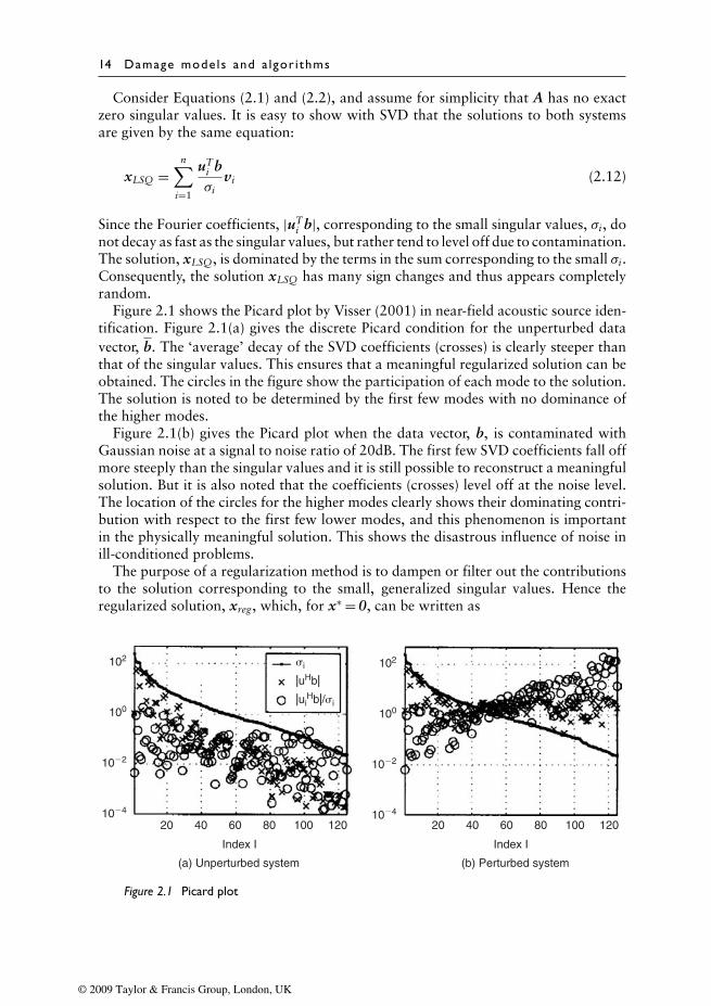
Figure 2.1 shows the Picard plot by Visser (2001) in near-field acoustic source iden-tification. Figure 2.1(a) gives the discrete Picard condition for the unperturbed datavector, b. The ‘average’ decay of the SVD coefficients (crosses) is clearly steeper thanthat of the singular values. This ensures that a meaningful regularized solution can beobtained. The circles in the figure show the participation of each mode to the solution.The solution is noted to be determined by the first few modes with no dominance ofthe higher modes.
Figure 2.1(b) gives the Picard plot when the data vector, b, is contaminated withGaussian noise at a signal to noise ratio of 20dB. The first few SVD coefficients fall offmore steeply than the singular values and it is still possible to reconstruct a meaningfulsolution. But it is also noted that the coefficients (crosses) level off at the noise level.The location of the circles for the higher modes clearly shows their dominating contri-bution with respect to the first few lower modes, and this phenomenon is importantin the physically meaningful solution. This shows the disastrous influence of noise inill-conditioned problems.
The purpose of a regularization method is to dampen or filter out the contributionsto the solution corresponding to the small, generalized singular values. Hence theregularized solution, xreg, which, for x∗ = 0, can be written as
102
100
10�2
10�4
102
100
�i
�uHb�
�uiHb�/�i
10�2
10�4
20 40 60
Index I
(a) Unperturbed system (b) Perturbed system
80 100 120 20 40 60
Index I
80 100 120
Figure 2.1 Picard plot
© 2009 Taylor & Francis Group, London, UK
Mathemat ica l concepts for d i screte inverse prob lems 15
xreg =n∑
i=1
fiuT
i bσi
vi if L = In (2.13)
xreg =p∑
i=1
fiuT
i bσi
xi +n∑
i=p+1
(uTi b)xi if L = In (2.14)
Here, the terms fi are the filter factors for the particular regularization method. Thefilter factors have the important property that as σi decreases, the corresponding fi
tends to zero in such a way that the contributions (uTi b/σi)xi to the solution from the
smaller σi are effectively filtered out. The difference between the various regulariza-tion methods lies essentially in the way these filter factors, fi, are defined. Hence, thefilter factors play an important role in regularization theory, and it is worthwhile char-acterizing the filter factors for the various regularization methods that are presentedbelow.
For Tikhonov regularization, which plays a central role in regularization theory, thefilter factors are either fi = σ2
i /(σ2i + λ2) (for L = In) or fi = γ2
i /(γ2i + λ2) (for L = In)
and the filtering effectively sets in for σi <λ and γi <λ, respectively. This shows thatthe discrete ill-posed problems are essentially un-regularized by Tikhonov’s methodfor λ<σn and λ<γp, respectively.
2.4 Solution by optimization
The detection and identification of structural damage is formulated as an optimiza-tion problem. The mathematical model of a physical structural system is establishedto fit the behaviour of a real system through minimizing the discrepancy betweenthe computed and measured responses. Many methods have been developed to solvethe optimization problem. Three of these methods are discussed here: gradient-basedapproach, genetic algorithm (GA) and simulated annealing.
2.4.1 Gradient-based approach
Many excellent and comprehensive texts on mathematical optimization have beenwritten, particularly in gradient-based algorithms (Snyman, 2005). Gradient-basedoptimization strategies iteratively search a minimum of an n-dimensional objectivefunction f (x). For the function f (x) ∈ C2, a vector of first-order partial derivatives, ora gradient vector can be computed at any point x, such that
∇f (x) =
∂f (x)∂x1
∂f (x)∂x2...
∂f (x)∂xn
= g(x) (2.15)
© 2009 Taylor & Francis Group, London, UK
16 Damage mode ls and a lgor i thms
where x = [x1, x2, · · · , xn]T ∈ �n. The actual optimization can be performed iteratively,and details of the iteration of the optimization problem by a gradient search techniqueare given below (Snyman, 2005):
(1) Given starting points x0 and positive tolerances ε1, ε2 and ε3, set i = 1.(2) Select a descent direction, pi.(3) Perform a linear search in direction pi to give the step size, λi.(4) Set xi = xi−1 + λi · pi and compute the objective function, f (xi).(5) Check the convergence criterion of f (xi). The algorithm is terminated if a conver-
gence criterion is satisfied. Termination is usually enforced at iteration i if one,or a combination, of the following criteria is met:
a) ‖xi − xi−1‖ < ε1; b) ‖∇f (xi)‖ < ε2; c) ‖f (xi) − f (xi−1)‖ < ε3.
(6) Set i = i + 1 and go back to Step 2.
To compute the step direction, pi, a linear (first-order) approximation of the objectivefunction can be used:
f (xi + λipi) ≈ f (xi) + (∇f (xi))Tpi (2.16)
which results in the step direction:
pi = −∇f (xi) (2.17)
This is called the steepest descent method. A second-order approach uses a quadraticapproximation:
∇f (xi) + ∇2f (xi)pi = 0 (2.18)
and this is referred to as the Newton’s direction method.For an analytical objective function, the first and second derivatives can be directly
transferred to a computer program. However if no explicit formula can be defined, theobjective function is computed numerically by means of a simulation where approxi-mations for the derivatives are necessary. The finite difference approximation can beapplied for each dimension for a multivariate objective function. The gradient vectorcan be approximated by the forward finite differences as
∂f (x)∂xj
∼= �f (x)δj
= f (x + δj) − f (x)δj
(2.19)
where δj = {0, 0, · · · , δj, 0, · · · , 0}T , δj > 0 at the j-th position. Better approximationsmay be obtained using central finite differences.
The performance of a gradient-based method strongly depends on the availableinitial values. Several optimization runs with different initial values might be necessaryif no a priori knowledge (e.g. the result of a process simulation) on the function to beoptimized is available.
© 2009 Taylor & Francis Group, London, UK
Mathemat ica l concepts for d i screte inverse prob lems 17
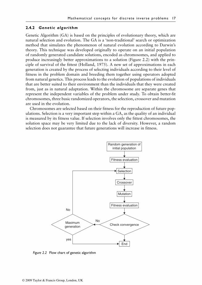
2.4.2 Genetic algorithm
Genetic Algorithm (GA) is based on the principles of evolutionary theory, which arenatural selection and evolution. The GA is a ‘non-traditional’ search or optimizationmethod that simulates the phenomenon of natural evolution according to Darwin’stheory. This technique was developed originally to operate on an initial populationof randomly generated candidate solutions, encoded as chromosomes, and applied toproduce increasingly better approximations to a solution (Figure 2.2) with the prin-ciple of survival of the fittest (Holland, 1975). A new set of approximations in eachgeneration is created by the process of selecting individuals according to their level offitness in the problem domain and breeding them together using operators adoptedfrom natural genetics. This process leads to the evolution of populations of individualsthat are better suited to their environment than the individuals that they were createdfrom, just as in natural adaptation. Within the chromosome are separate genes thatrepresent the independent variables of the problem under study. To obtain better-fitchromosomes, three basic randomized operators, the selection, crossover and mutationare used in the evolution.
Chromosomes are selected based on their fitness for the reproduction of future pop-ulations. Selection is a very important step within a GA, as the quality of an individualis measured by its fitness value. If selection involves only the fittest chromosomes, thesolution space may be very limited due to the lack of diversity. However, a randomselection does not guarantee that future generations will increase in fitness.
Random generation ofinitial population
Fitness evaluation
Selection
Crossover
Mutation
Fitness evaluation
Check convergence
End
NoMaximumgeneration
No
yes
Figure 2.2 Flow chart of genetic algorithm
© 2009 Taylor & Francis Group, London, UK
18 Damage mode ls and a lgor i thms
Crossover is the most important operator in a GA. This operator takes thechromosomes of two parents which are randomly selected, and then exchanges part oftheir genes resulting in two new chromosomes for the child generation. Therefore, thecrossover does not create new material within the population; it simply inter-mixes theexisting population. The usual schemes to generate new chromosomes are the single-point crossover, the multipoint crossover and the uniform crossover. The probabilityof crossover defines the ratio of the number of offspring produced in each generationto the population size.
The mutation operator introduces a change in one or more of the chromosome’sgenes. New material is introduced in the population with this operator and its maingoal is to prevent the population from converging to a local minimum. The probabilityof mutation is defined as the ratio of the number of mutated genes to the total numberof genes in the population and its value is usually low, typically in the range 0.01 and0.001. However, in some cases it can take higher values with the purpose of increasingthe diversity of the population.
From the above discussion, it can be seen that GAs differ substantially from tradi-tional gradient-based search techniques. In fact, they have several advantages that makethem suitable for dealing with complex problems where traditional search techniquesfail. The major advantages are:
• GAs work on a population of points in parallel in the search space, while tradi-tional search techniques work only on a single point at a time. Because of this,the guess of the initial point has a large effect in traditional methods, since thereis a possibility of converging to a local optimal point rather than the global opti-mal point. Therefore, GAs are more advantageous in complex, nonlinear andmultimodal optimization problems.
• GAs, unlike traditional optimization techniques, do not require the evaluationof gradients or higher-order derivatives. Only the objective function and thecorresponding fitness levels influence the directions of search. Therefore, GAsare applicable in problems where the objective function is not differentiable.
• GAs use probabilistic search rules, not deterministic ones like gradient-basedoptimization.
• GAs work on an encoding of the parameter set rather than the parameter itself(except for where real-valued individuals are used).
Due to all these advantages, GAs, although slow in execution, are best applied toproblems where traditional optimization techniques do not work well, as in the case ofcomplex problems with many local optima and where the global optimum is required.However, the main disadvantage of GAs, compared to traditional methods, is their highcomputational cost. However, this drawback can be overcome with faster computersor by using simple objective functions that can be quickly computed. In addition, GAsare not suitable for problems with too many variables, since the search space becomesmuch larger with an increase in the number of variables. In these cases, GAs appearto be relatively imprecise in performance near to the global optimum when comparedwith conventional optimization techniques.
© 2009 Taylor & Francis Group, London, UK
Mathemat ica l concepts for d i screte inverse prob lems 19
2.4.3 Simulated anneal ing
Another important computational intelligence approach, simulated annealing (SA), is apopular stochastic method based on the physical process of annealing (Van Laarhovenand Aarts, 1987). SA is the simulation of the annealing of a physical multi-particlesystem for finding the global optimum solution of a large combinatorial optimizationproblem. If a system is in a configuration q at time t, then a new configuration r of thesystem at time t + 1 is generated randomly. The configuration r is accepted accordingto the acceptance probability Pro(r).
Pr o(r) = e−(
Er−EqKBT
)(2.20)
where KB is the Boltzmann constant and T is referred to as control parameter (ortemperature in the original SA). The energy of the original configuration q and thenew configuration r is represented as Eq and Er, respectively. In addition, an annealingprocess is needed to obtain a lower energy configuration. The well-known coolingschedule that provides the necessary and sufficient conditions for convergence is
C(t) = C0
log t∀t > 0 (2.21)
where C(t) is a sequence of control parameters, C0 is a constant and t is the time. It isnoted that C(t) approaches zero when t goes to infinity.
When the simulated annealing schedule is applied to an optimization problem, theenergy function becomes the objective function, and the configuration becomes thesolution configuration of the parameters. Also Equations (2.20) and (2.21) can befurther transformed as
Pr o(r) = e−(
Er−EqT(l)
)(2.22)
T(l) = Tlog l
(2.23)
where l denotes an integer step sequence, T0 is the initial constant control parameterand T(l) is a sequence of control parameter. Equations (2.22) and (2.23) then give
Pr o(l) = l−(
Er−EqT0
)(2.24)
It is noted that Pro(l) equals 1.0 when l = 1.0.
2.5 Tikhonov regularization
Regularization techniques include direct regularization methods and iterative regular-ization methods. A brief review of the regularization methods for numerical treatmentof discrete ill-posed problems is found in Hansen (1994). Equation. (2.3) shows thatthe zeroth-order regularization when L = I (the identify matrix). It becomes the first-order regularization when L is a gradient operator and a second-order regularization
© 2009 Taylor & Francis Group, London, UK
20 Damage mode ls and a lgor i thms
when L is a surface Laplacian operator. Only one of the three orders of regularizationis employed under most circumstances. The zeroth-order regularization biases theestimates towards zero but also greatly reduces large-magnitude oscillations in theparameter values, whereas first-order regularization biases the estimates towards aconstant and reduces the tendency to fluctuate from one value to the next. Threeregularization methods (truncated SVD, generalized cross-validation and L-curve) arediscussed in the following sections.
2.5.1 Truncated singular value decomposit ion
The SVD allows the solution of singular systems by separating the components ofoperators belonging to its range from those belonging to its null-space (correspondingto the null singular values). If the whole set of n singular values in Equation (2.4) isnonzero, the solution becomes:
x =n∑
i=1
σ−1i (uT
i b)vi (2.25)
The small singular values may cause solution instability as discussed in Section 2.3.1,and the terms corresponding to the smallest singular values are affected. It wouldbe useful to consider these terms as belonging to the null-space and neglecting thecorresponding singular values. In this way, the solution is deprived of some informationcontent but becomes more regular without solution instability due to the small singularvalues. This is one way to treat the ill-conditioning of A to generate a new problemwith a well-conditioned rank deficient coefficient matrix. The rank deficient matrix,which is the closest rank-k approximation Ak to A, is measured in the 2-norm and isobtained by truncating the SVD expansion in Equation (2.4) at k, to give
Ak =k∑
i=1
uiσivTi , k ≤ n (2.26)
and the solution is given by
xk =k∑
i=1
uTi bσi
vi (2.27)
The number of neglected singular values should be neither too high to preserve theinformation content, nor too low to obtain a more stable solution. If an estimate,‖δb‖, of the amount of noise in the data is available, the summation in Equation (2.25)can be truncated when the following condition is not satisfied:
σk ≥ ‖δb‖ σ1 (2.28)
This means that the first k singular values can be retained when error in the data canbe removed by filtering.
An alternative method to treat the problem is to use the discrete Picard conditionto determine the number of terms in the summation in Equation. (2.12). Since the
© 2009 Taylor & Francis Group, London, UK
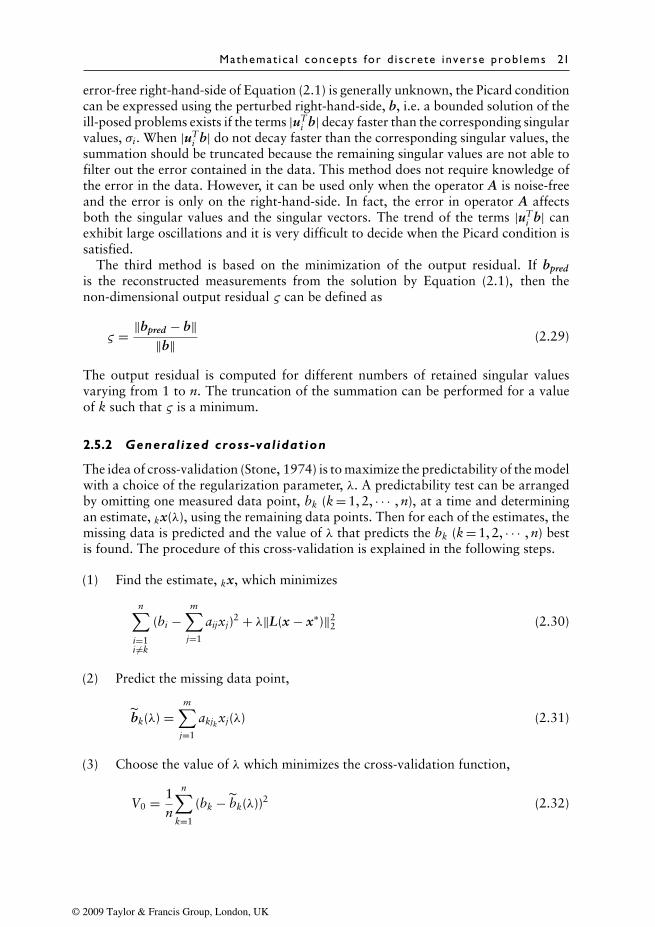
Mathemat ica l concepts for d i screte inverse prob lems 21
error-free right-hand-side of Equation (2.1) is generally unknown, the Picard conditioncan be expressed using the perturbed right-hand-side, b, i.e. a bounded solution of theill-posed problems exists if the terms |uT
i b| decay faster than the corresponding singularvalues, σi. When |uT
i b| do not decay faster than the corresponding singular values, thesummation should be truncated because the remaining singular values are not able tofilter out the error contained in the data. This method does not require knowledge ofthe error in the data. However, it can be used only when the operator A is noise-freeand the error is only on the right-hand-side. In fact, the error in operator A affectsboth the singular values and the singular vectors. The trend of the terms |uT
i b| canexhibit large oscillations and it is very difficult to decide when the Picard condition issatisfied.
The third method is based on the minimization of the output residual. If bpredis the reconstructed measurements from the solution by Equation (2.1), then thenon-dimensional output residual ς can be defined as
ς = ‖bpred − b‖‖b‖ (2.29)
The output residual is computed for different numbers of retained singular valuesvarying from 1 to n. The truncation of the summation can be performed for a valueof k such that ς is a minimum.
2.5.2 General ized cross-val idation
The idea of cross-validation (Stone, 1974) is to maximize the predictability of the modelwith a choice of the regularization parameter, λ. A predictability test can be arrangedby omitting one measured data point, bk (k = 1, 2, · · · , n), at a time and determiningan estimate, kx(λ), using the remaining data points. Then for each of the estimates, themissing data is predicted and the value of λ that predicts the bk (k = 1, 2, · · · , n) bestis found. The procedure of this cross-validation is explained in the following steps.
(1) Find the estimate, kx, which minimizes
n∑i=1i =k
(bi −m∑
j=1
aijxj)2 + λ‖L(x − x∗)‖22 (2.30)
(2) Predict the missing data point,
bk(λ) =m∑
j=1
akjkxj(λ) (2.31)
(3) Choose the value of λ which minimizes the cross-validation function,
V0 = 1n
n∑k=1
(bk − bk(λ))2 (2.32)
© 2009 Taylor & Francis Group, London, UK
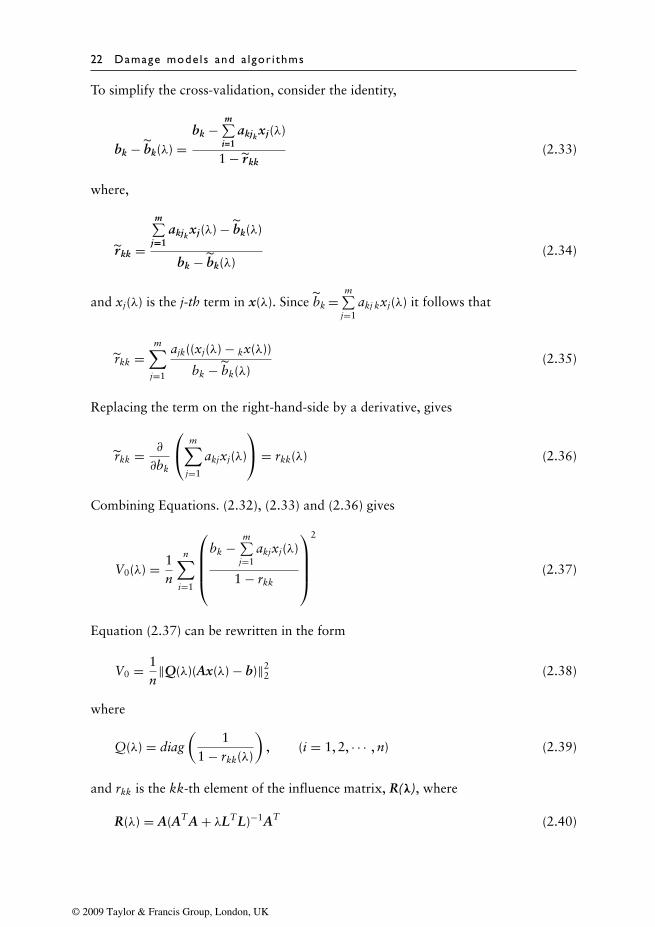
22 Damage mode ls and a lgor i thms
To simplify the cross-validation, consider the identity,
bk − bk(λ) =bk −
m∑i=1
akjkxj(λ)
1 − r kk(2.33)
where,
r kk =
m∑j=1
akjkxj(λ) − bk(λ)
bk − bk(λ)(2.34)
and xj(λ) is the j-th term in x(λ). Since bk =m∑
j=1akj kxj(λ) it follows that
rkk =m∑
j=1
ajk((xj(λ) − kx(λ))
bk − bk(λ)(2.35)
Replacing the term on the right-hand-side by a derivative, gives
rkk = ∂
∂bk
m∑j=1
akjxj(λ)
= rkk(λ) (2.36)
Combining Equations. (2.32), (2.33) and (2.36) gives
V0(λ) = 1n
n∑i=1
bk −
m∑j=1
akjxj(λ)
1 − rkk
2
(2.37)
Equation (2.37) can be rewritten in the form
V0 = 1n
‖Q(λ)(Ax(λ) − b)‖22 (2.38)
where
Q(λ) = diag(
11 − rkk(λ)
), (i = 1, 2, · · · , n) (2.39)
and rkk is the kk-th element of the influence matrix, R(λ), where
R(λ) = A(ATA + λLTL)−1AT (2.40)
© 2009 Taylor & Francis Group, London, UK
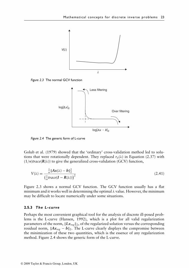
Mathemat ica l concepts for d i screte inverse prob lems 23
V(λ)
λ
Figure 2.3 The normal GCV function
log�Lx�2
Less filtering
Over filtering
log�Ax � b�2
Figure 2.4 The generic form of L-curve
Golub et al. (1979) showed that the ‘ordinary’ cross-validation method led to solu-tions that were rotationally dependent. They replaced rii(λ) in Equation (2.37) with(1/n)trace(R(λ)) to give the generalized cross-validation (GCV) function,
V(λ) =1n‖Ax(λ) − b‖2
2( 1n trace(I − R(λ))
)2 (2.41)
Figure 2.3 shows a normal GCV function. The GCV function usually has a flatminimum and it works well in determining the optimal λ value. However, the minimummay be difficult to locate numerically under some situations.
2.5.3 The L-curve
Perhaps the most convenient graphical tool for the analysis of discrete ill-posed prob-lems is the L-curve (Hansen, 1992), which is a plot for all valid regularizationparameters of the norm, ‖Lxreg‖2, of the regularized solution versus the correspondingresidual norm, ‖Axreg − b‖2. The L-curve clearly displays the compromise betweenthe minimization of these two quantities, which is the essence of any regularizationmethod. Figure 2.4 shows the generic form of the L-curve.
© 2009 Taylor & Francis Group, London, UK
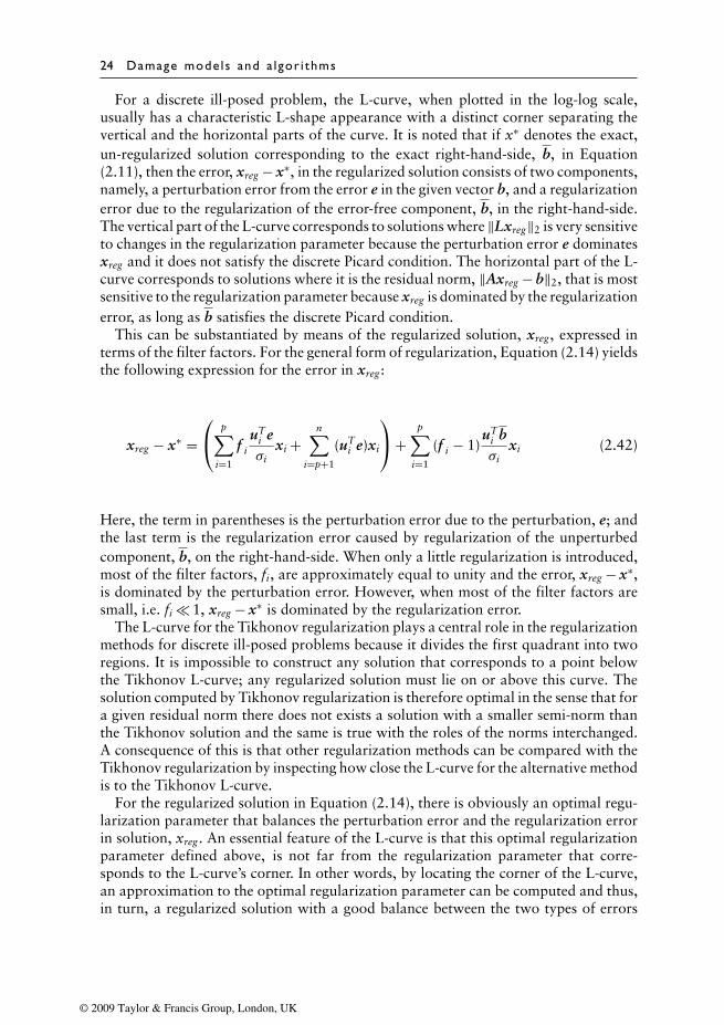
24 Damage mode ls and a lgor i thms
For a discrete ill-posed problem, the L-curve, when plotted in the log-log scale,usually has a characteristic L-shape appearance with a distinct corner separating thevertical and the horizontal parts of the curve. It is noted that if x∗ denotes the exact,un-regularized solution corresponding to the exact right-hand-side, b, in Equation(2.11), then the error, xreg − x∗, in the regularized solution consists of two components,namely, a perturbation error from the error e in the given vector b, and a regularizationerror due to the regularization of the error-free component, b, in the right-hand-side.The vertical part of the L-curve corresponds to solutions where ‖Lxreg‖2 is very sensitiveto changes in the regularization parameter because the perturbation error e dominatesxreg and it does not satisfy the discrete Picard condition. The horizontal part of the L-curve corresponds to solutions where it is the residual norm, ‖Axreg − b‖2, that is mostsensitive to the regularization parameter because xreg is dominated by the regularizationerror, as long as b satisfies the discrete Picard condition.
This can be substantiated by means of the regularized solution, xreg, expressed interms of the filter factors. For the general form of regularization, Equation (2.14) yieldsthe following expression for the error in xreg:
xreg − x∗ = p∑
i=1
f iuT
i eσi
xi +n∑
i=p+1
(uTi e)xi
+p∑
i=1
(f i − 1)uT
i bσi
xi (2.42)
Here, the term in parentheses is the perturbation error due to the perturbation, e; andthe last term is the regularization error caused by regularization of the unperturbedcomponent, b, on the right-hand-side. When only a little regularization is introduced,most of the filter factors, fi, are approximately equal to unity and the error, xreg − x∗,is dominated by the perturbation error. However, when most of the filter factors aresmall, i.e. fi 1, xreg − x∗ is dominated by the regularization error.
The L-curve for the Tikhonov regularization plays a central role in the regularizationmethods for discrete ill-posed problems because it divides the first quadrant into tworegions. It is impossible to construct any solution that corresponds to a point belowthe Tikhonov L-curve; any regularized solution must lie on or above this curve. Thesolution computed by Tikhonov regularization is therefore optimal in the sense that fora given residual norm there does not exists a solution with a smaller semi-norm thanthe Tikhonov solution and the same is true with the roles of the norms interchanged.A consequence of this is that other regularization methods can be compared with theTikhonov regularization by inspecting how close the L-curve for the alternative methodis to the Tikhonov L-curve.
For the regularized solution in Equation (2.14), there is obviously an optimal regu-larization parameter that balances the perturbation error and the regularization errorin solution, xreg. An essential feature of the L-curve is that this optimal regularizationparameter defined above, is not far from the regularization parameter that corre-sponds to the L-curve’s corner. In other words, by locating the corner of the L-curve,an approximation to the optimal regularization parameter can be computed and thus,in turn, a regularized solution with a good balance between the two types of errors
© 2009 Taylor & Francis Group, London, UK

Mathemat ica l concepts for d i screte inverse prob lems 25
can be computed. For continuous L-curves, a computationally convenient definitionof the L-curve’s corner is the point with maximum curvature in the log-log scale.
max(log‖Axλ − b‖2, log‖Lxλ‖2) (2.43)
When the regularization parameter is discrete, the discrete L-curve in the log-log scalecan be approximated by a two-dimensional spline curve. The point on the spline curvewith maximum curvature was computed and the corner of the discrete L-curve at thatpoint, which is closest to the corner of the spline curve, was defined.
2.6 General optimization procedure for theinverse problem
The procedure of a general iterative algorithm used to solve the nonlinear optimizationproblem is as follows:
1) Initially assume x0.2) Since the measurements of the baseline model are not available, they are calculated
using the theoretical model instead of the measured information.3) Solve the inverse problem using one of the optimization procedures.4) Reconstruct the responses using the identified results.5) Calculate the criteria of convergence in Equation (2.44). Convergence is achieved
when the errors are less than the predefined tolerance values.6) When the computed error does not converge, repeat Steps 3 to 5 until convergence
is reached.
2.7 The criteria of convergence
The usual criteria of convergence are
Error1 = ‖b − bPr edicted‖
‖U s‖ × 100%
Error2 = ‖xj+1 − xj‖‖xj‖ × 100%
(2.44)
The first criterion is based on the output residual between the measurements and thereconstructed responses. The second criterion is based on the difference between theidentified results of two adjacent steps.
2.8 Summary
This chapter gives a brief description of the basic knowledge of ill-posed inverse prob-lems and three optimization algorithms for the solution of inverse problems. Thetechniques to obtain the regularization solution are discussed and these techniquesare used in the following chapters for the condition assessment of structures.
© 2009 Taylor & Francis Group, London, UK
Chapter 3
Damage description and modelling
3.1 Introduction
3.1.1 Damage models
The following two questions are often asked: Where does the damage occur? And whatis its magnitude? In fact, there may be many types of damage due to various reasonsover the lifetime of the structure, and they affect the structural dynamic characteristicsdifferently. The error in modelling the damage itself plays a significant role in thedamage detection process. A more satisfactory set of question would be: Where doesthe damage occur? What kind of damage it is? And what is its magnitude? Manydamage detection methods take the local damage as an overall reduction in the localstiffness of an element. Efforts have been made to build damage models but most ofthem are related to cracks in a beam. More comprehensive damage models with cracksin a plate have also been formulated based on the constitutive relations. If the initialmodel is not provided with the description of a particular type of damage, then thesubsequent model improvement cannot yield the correct description of the damage inthe finite element. A good example is the model error of a Timoshenko beam, where theinitial model is based on that of an Euler–Bernoulli beam. Condition assessment basedon an incorrect description of the damage yields system errors that spread throughoutthe identified results, and they account for a significant portion of the total error inthe result.
3.1.2 Model on pre-stress
The load-carrying capacity of a pre-stressed structure depends mainly on the levelof pre-stress in the structure. A significant reduction in the pre-stress jeopardizes thesafety level of the structure. The modelling of pre-stress at the design stage is basedon an equilibrating force system from which the internal stresses are calculated. Sucha model is useful when static measured data are used for the system identification of thestructure. But when dynamic data are used, the restoring forces from the equilibratingforce system always tend to zero with no indication of the level of pre-stress. Twomodels of the pre-stress in a structure are given in this chapter with the pre-stressingeffect modelled as physical parameters in the structural system, and they are speciallydeveloped for structural damage detection.
© 2009 Taylor & Francis Group, London, UK
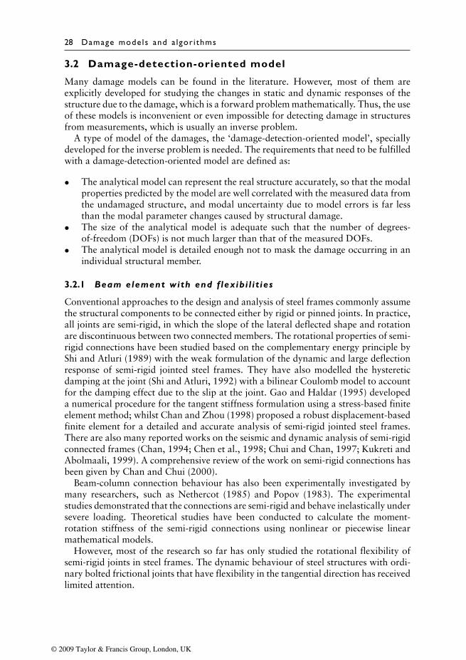
28 Damage mode ls and a lgor i thms
3.2 Damage-detection-oriented model
Many damage models can be found in the literature. However, most of them areexplicitly developed for studying the changes in static and dynamic responses of thestructure due to the damage, which is a forward problem mathematically. Thus, the useof these models is inconvenient or even impossible for detecting damage in structuresfrom measurements, which is usually an inverse problem.
A type of model of the damages, the ‘damage-detection-oriented model’, speciallydeveloped for the inverse problem is needed. The requirements that need to be fulfilledwith a damage-detection-oriented model are defined as:
• The analytical model can represent the real structure accurately, so that the modalproperties predicted by the model are well correlated with the measured data fromthe undamaged structure, and modal uncertainty due to model errors is far lessthan the modal parameter changes caused by structural damage.
• The size of the analytical model is adequate such that the number of degrees-of-freedom (DOFs) is not much larger than that of the measured DOFs.
• The analytical model is detailed enough not to mask the damage occurring in anindividual structural member.
3.2.1 Beam element with end flexibi l i t ies
Conventional approaches to the design and analysis of steel frames commonly assumethe structural components to be connected either by rigid or pinned joints. In practice,all joints are semi-rigid, in which the slope of the lateral deflected shape and rotationare discontinuous between two connected members. The rotational properties of semi-rigid connections have been studied based on the complementary energy principle byShi and Atluri (1989) with the weak formulation of the dynamic and large deflectionresponse of semi-rigid jointed steel frames. They have also modelled the hystereticdamping at the joint (Shi and Atluri, 1992) with a bilinear Coulomb model to accountfor the damping effect due to the slip at the joint. Gao and Haldar (1995) developeda numerical procedure for the tangent stiffness formulation using a stress-based finiteelement method; whilst Chan and Zhou (1998) proposed a robust displacement-basedfinite element for a detailed and accurate analysis of semi-rigid jointed steel frames.There are also many reported works on the seismic and dynamic analysis of semi-rigidconnected frames (Chan, 1994; Chen et al., 1998; Chui and Chan, 1997; Kukreti andAbolmaali, 1999). A comprehensive review of the work on semi-rigid connections hasbeen given by Chan and Chui (2000).
Beam-column connection behaviour has also been experimentally investigated bymany researchers, such as Nethercot (1985) and Popov (1983). The experimentalstudies demonstrated that the connections are semi-rigid and behave inelastically undersevere loading. Theoretical studies have been conducted to calculate the moment-rotation stiffness of the semi-rigid connections using nonlinear or piecewise linearmathematical models.
However, most of the research so far has only studied the rotational flexibility ofsemi-rigid joints in steel frames. The dynamic behaviour of steel structures with ordi-nary bolted frictional joints that have flexibility in the tangential direction has receivedlimited attention.
© 2009 Taylor & Francis Group, London, UK
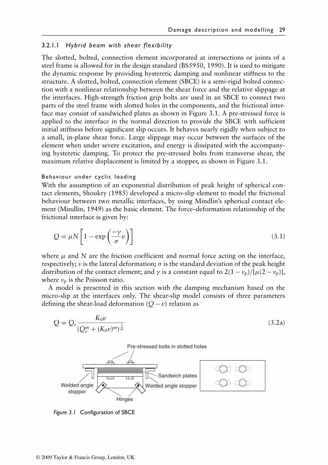
Damage descr ipt ion and mode l l ing 29
3.2.1.1 Hybr id beam with shear f lex ib i l i t y
The slotted, bolted, connection element incorporated at intersections or joints of asteel frame is allowed for in the design standard (BS5950, 1990). It is used to mitigatethe dynamic response by providing hysteretic damping and nonlinear stiffness to thestructure. A slotted, bolted, connection element (SBCE) is a semi-rigid bolted connec-tion with a nonlinear relationship between the shear force and the relative slippage atthe interfaces. High-strength friction grip bolts are used in an SBCE to connect twoparts of the steel frame with slotted holes in the components, and the frictional inter-face may consist of sandwiched plates as shown in Figure 3.1. A pre-stressed force isapplied to the interface in the normal direction to provide the SBCE with sufficientinitial stiffness before significant slip occurs. It behaves nearly rigidly when subject toa small, in-plane shear force. Large slippage may occur between the surfaces of theelement when under severe excitation, and energy is dissipated with the accompany-ing hysteretic damping. To protect the pre-stressed bolts from transverse shear, themaximum relative displacement is limited by a stopper, as shown in Figure 3.1.
Behav iour under cyc l i c load ingWith the assumption of an exponential distribution of peak height of spherical con-tact elements, Shoukry (1985) developed a micro-slip element to model the frictionalbehaviour between two metallic interfaces, by using Mindlin’s spherical contact ele-ment (Mindlin, 1949) as the basic element. The force–deformation relationship of thefrictional interface is given by:
Q = µN[1 − exp
(−γσ
v)]
(3.1)
where µ and N are the friction coefficient and normal force acting on the interface,respectively; ν is the lateral deformation; σ is the standard deviation of the peak heightdistribution of the contact element; and γ is a constant equal to 2(1 − νp)/[µ(2 − νp)],where νp is the Poisson ratio.
A model is presented in this section with the damping mechanism based on themicro-slip at the interfaces only. The shear-slip model consists of three parametersdefining the shear-load deformation (Q − v) relation as
Q = QsK0v
(Qms + (K0v)m)
1m
(3.2a)
Sandwich plates
Pre-stressed bolts in slotted holes
Hinges
Welded anglestopper
Welded angle stopper
Figure 3.1 Configuration of SBCE
© 2009 Taylor & Francis Group, London, UK
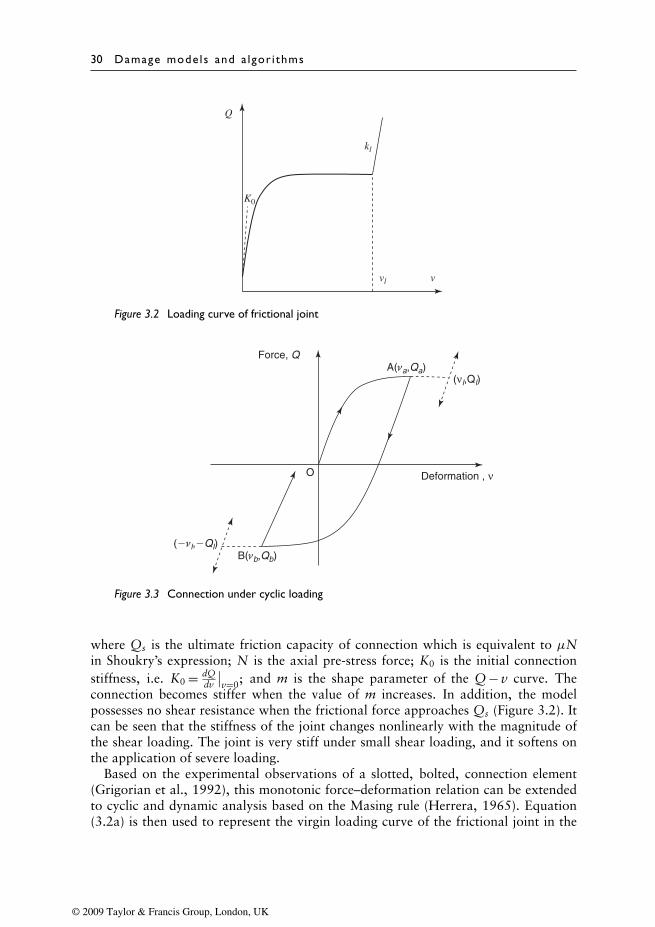
30 Damage mode ls and a lgor i thms
Q
K0
kl
vl v
Figure 3.2 Loading curve of frictional joint
Force, Q
O
B(νb,Qb)
A(νa,Qa)(νl,Ql)
(�νl,�Ql)
Deformation , ν
Figure 3.3 Connection under cyclic loading
where Qs is the ultimate friction capacity of connection which is equivalent to µNin Shoukry’s expression; N is the axial pre-stress force; K0 is the initial connectionstiffness, i.e. K0 = dQ
dv
∣∣v=0; and m is the shape parameter of the Q − v curve. The
connection becomes stiffer when the value of m increases. In addition, the modelpossesses no shear resistance when the frictional force approaches Qs (Figure 3.2). Itcan be seen that the stiffness of the joint changes nonlinearly with the magnitude ofthe shear loading. The joint is very stiff under small shear loading, and it softens onthe application of severe loading.
Based on the experimental observations of a slotted, bolted, connection element(Grigorian et al., 1992), this monotonic force–deformation relation can be extendedto cyclic and dynamic analysis based on the Masing rule (Herrera, 1965). Equation(3.2a) is then used to represent the virgin loading curve of the frictional joint in the
© 2009 Taylor & Francis Group, London, UK

Damage descr ipt ion and mode l l ing 31
tangential direction. The corresponding instantaneous connection stiffness in the virgincurve is given by
rv = dQdvc
= K0
[1 − Qm
Qms
]m+1m
= K0
[1 − (K0v)m
(K0v)m + Qms
]m+1m
(3.2b)
Equation (3.2a) can also be generalized for both the unloading and reloading curves,based on the Masing rule as∣∣∣∣Q − Q∗
2
∣∣∣∣ = QsK0
∣∣ v − v∗2
∣∣(Qm
s + (K0
∣∣ v − v∗2
∣∣)m) 1m
(3.3a)
where (v∗, Q∗) is the point at which the load reversal occurs at point A in Figure 3.3.Therefore, the corresponding instantaneous connection stiffness of both the unloadingand reloading curves can be expressed as
rv = dQdv
= K0
1 −∣∣∣Q − Q∗
2
∣∣∣mQm
s
m+1
m
= K0
[1 −
(K0
∣∣ v − v∗2
∣∣)m(K0
∣∣ v − v∗2
∣∣)m + Qms
]m+1m
(3.3b)
in which, v∗ = v∗a when the slippage deformation happens at the reversal point A in
Figure 3.3. If point B is the next reversal point, the reloading stiffness is obtained byreplacing v∗
a with v∗b in Equation (3.3b).
Equations (3.2a and 3.2b) are physically important because the joint parameters inthe loading curve, such as the initial stiffness and the frictional resistance force, arerelated to other physical parameters, such as the normal pressure and friction coeffi-cient. Accordingly, the joint properties can be predicted from other physical parame-ters, and direct testing for the force–deformation characteristics may not be necessary.
In the following formulation, Equation (3.2b) is used to represent the virginloading curve of the frictional joint in the tangential direction. The correspondinginstantaneous connection stiffness in the virgin curve is given by
rv = dQdvc
= K0 exp[−K0
Qsvc
], if |vc| ≤ vcl;
rv = dQdvc
= kl, if |vc| > vcl;
(3.4)
Equation (3.2a) can also be generalized for both the unloading and reloading curves,based on the Masing rule as
∣∣∣∣Q − Q∗
2
∣∣∣∣ = Qs
[1 − exp
(−K0
Qs
∣∣∣∣vc − v∗c
2
∣∣∣∣)] , if |vc| ≤ vcl;
Q = Q∗ + kl(vc − v∗c ), if |vc| > vcl;
(3.5)
© 2009 Taylor & Francis Group, London, UK
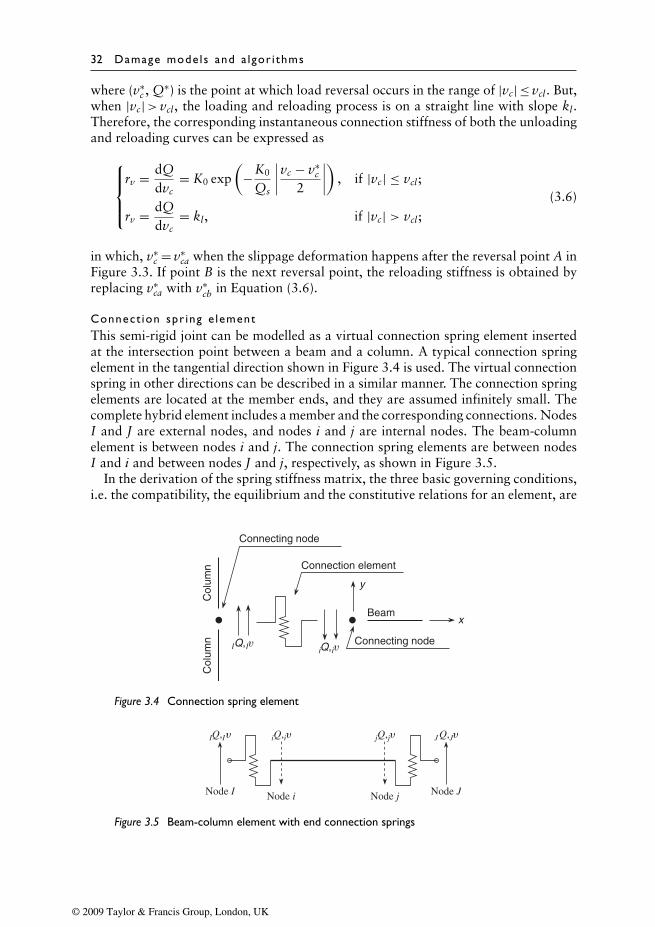
32 Damage mode ls and a lgor i thms
where (v∗c , Q∗) is the point at which load reversal occurs in the range of |vc| ≤ vcl. But,
when |vc|> vcl, the loading and reloading process is on a straight line with slope kl.Therefore, the corresponding instantaneous connection stiffness of both the unloadingand reloading curves can be expressed as
rv = dQdvc
= K0 exp(
−K0
Qs
∣∣∣∣vc − v∗c
2
∣∣∣∣) , if |vc| ≤ vcl;
rv = dQdvc
= kl, if |vc| > vcl;
(3.6)
in which, v∗c = v∗
ca when the slippage deformation happens after the reversal point A inFigure 3.3. If point B is the next reversal point, the reloading stiffness is obtained byreplacing v∗
ca with v∗cb in Equation (3.6).
Connect ion spr ing e lementThis semi-rigid joint can be modelled as a virtual connection spring element insertedat the intersection point between a beam and a column. A typical connection springelement in the tangential direction shown in Figure 3.4 is used. The virtual connectionspring in other directions can be described in a similar manner. The connection springelements are located at the member ends, and they are assumed infinitely small. Thecomplete hybrid element includes a member and the corresponding connections. NodesI and J are external nodes, and nodes i and j are internal nodes. The beam-columnelement is between nodes i and j. The connection spring elements are between nodesI and i and between nodes J and j, respectively, as shown in Figure 3.5.
In the derivation of the spring stiffness matrix, the three basic governing conditions,i.e. the compatibility, the equilibrium and the constitutive relations for an element, are
Connection element
Connecting node
Beam
Connecting node
Col
umn
Col
umn
x
y
IQ,Iυ iQ,iυ
Figure 3.4 Connection spring element
IQ,Iy iQ,iy jQ,jy J Q,Jy
Node I Node JNode i Node j
Figure 3.5 Beam-column element with end connection springs
© 2009 Taylor & Francis Group, London, UK
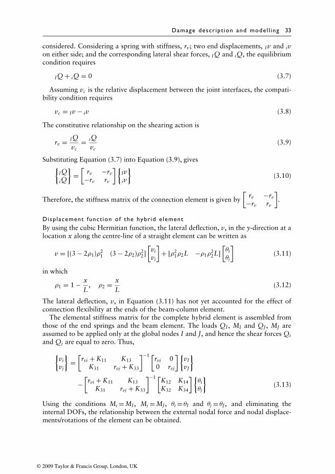
Damage descr ipt ion and mode l l ing 33
considered. Considering a spring with stiffness, rv; two end displacements, Iv and ivon either side; and the corresponding lateral shear forces, IQ and iQ, the equilibriumcondition requires
IQ + iQ = 0 (3.7)
Assuming vc is the relative displacement between the joint interfaces, the compati-bility condition requires
vc = Iv − iv (3.8)
The constitutive relationship on the shearing action is
rv = IQvc
= iQvc
(3.9)
Substituting Equation (3.7) into Equation (3.9), gives{IQiQ
}=[
rv −rv
−rv rv
]{Iviv
}(3.10)
Therefore, the stiffness matrix of the connection element is given by[
rv −rv
−rv rv
].
Disp lacement funct ion of the hybr id e lementBy using the cubic Hermitian function, the lateral deflection, v, in the y-direction at alocation x along the centre-line of a straight element can be written as
v = [(3 − 2ρ1)ρ21 (3 − 2ρ2)ρ2
2][vi
vj
]+ [ρ2
1ρ2L −ρ1ρ22L]
[θiθj
](3.11)
in which
ρ1 = 1 − xL
, ρ2 = xL
(3.12)
The lateral deflection, v, in Equation (3.11) has not yet accounted for the effect ofconnection flexibility at the ends of the beam-column element.
The elemental stiffness matrix for the complete hybrid element is assembled fromthose of the end springs and the beam element. The loads QI, MI and QJ, MJ areassumed to be applied only at the global nodes I and J, and hence the shear forces Qi
and Qj are equal to zero. Thus,{vi
vj
}=[rvi + K11 K13
K31 rvj + K33
]−1 [rvi 00 rvj
]{vI
vJ
}−[rvi + K11 K13
K31 rvj + K33
]−1 [K12 K14
K32 K34
]{θiθj
}(3.13)
Using the conditions Mi = MI, Mj = MJ, θi = θI and θj = θJ, and eliminating theinternal DOFs, the relationship between the external nodal force and nodal displace-ments/rotations of the element can be obtained.
© 2009 Taylor & Francis Group, London, UK
34 Damage mode ls and a lgor i thms
In assembling the elemental stiffness matrices of a structure, the element stiffnessmatrix is rewritten in the global coordinate system for geometrical compatibility. Sub-stituting Equation (3.13) into Equation (3.11) and transforming the external nodalrotations, θI and θJ, about the local axis at the ends of the element to the global nodalrotations θi and θj, the displacement function v can finally be written as
v = [(3 − 2ρ1)ρ21 (3 − 2ρ2)ρ2
2][rvi + K11 K13
K31 rvj + K33
]−1 [rvi 00 rvj
]{vI
vJ
}− [(3 − 2ρ1)ρ2
1 (3 − 2ρ2)ρ22][rvi + K11 K13
K31 rvj + K33
]−1 [K12 K14
K32 K34
]{θIθJ
}+ [ρ2
1ρ2L −ρ1ρ22L]
{θIθJ
}= [(3 − 2ρ1)ρ2
1 (3 − 2ρ2)ρ22][rvi + K11 K13
K31 rvj + K33
]−1 [rvi 00 rvj
]{vi
vj
}
+(
[ρ21ρ2L −ρ1ρ
22L] − [(3 − 2ρ1)ρ2
1 (3 − 2ρ2)ρ22]
×[rvi + K11 K13
K31 rvj + K33
]−1 [K12 K14
K32 K34
])[1/L 1 −1/L 01/L 0 −1/L 1
]vi
θi
vj
θj
(3.14)
in which vi, vj, θi and θj are the nodal displacements and rotations of the elementreferring to the global axis.
The displacement function, w, in the z-direction can also be expressed similar toEquation (3.14) when under the shear load and bending moments at the global DOFsat the ends of the member.
L inear e lementa l s t i f fness matr ixThe linear stiffness matrix, [KL], for a beam-column element in the x- and y-planescan be obtained based on the variational principle and the energy theorem,
[KL] =∫ L
0
(∂2v∂x2
)T
EI(∂2v∂x2
)dx (3.15)
The nonzero terms of the upper triangle of the linear stiffness matrix (in localcoordinates) of the three-dimensional element are
KL1,1 = EA/L, KL1,7 = −EA/L,
KL2,2 = 48EIzξ−1y (ry
vi)2(ry
vj)2, KL2,6 = 12EIzLξ−1
y (ryvi)
2(ryvj)
2,
KL2,8 = −48EIzξ−1y (ry
vi)2(ry
vj)2, KL2,12 = 12EIzLξ−1
y (ryvi)
2(ryvj)
2,
KL3,3 = 48EIyξ−1z (rz
vi)2(rz
vj)2, KL3,5 = 12EIyLξ−1
z (rzvi)
2(rzvj)
2,
© 2009 Taylor & Francis Group, London, UK
Damage descr ipt ion and mode l l ing 35
KL3,9 = −48EIyξ−1z (rz
vi)2(rz
vj)2, KL3,11 = 12EIyLξ−1
z (rzvi)
2(rzvj)
2,
KL4,4 = GJ/L, KL4,10 = −GJ/L,
KL5,5 = L2EIyξ−1z {(Kz
11)2(rzvi)
2 + 2(Kz11)2rz
virzvj + 2Kz
11(rzvi)
2rzvj
+ (Kz11)2(rz
vj)2 + 2Kz
11rzvi(r
zvj)
2 + 4(rzvi)
2(rzvj)
2},
KL5,9 = −12EIyLξ−1z (rz
vi)2(rz
vj)2,
KL5,11 = −L2EIyξ−1z {(Kz
11)2(rzvi)
2 + 2(Kz11)2rz
virzvj + 2Kz
11(rzvi)
2rzvj
+ (Kz11)2(rz
vj)2 + 2Kz
11rzvi(r
zvj)
2 − 2(rzvi)
2(rzvj)
2},
KL6,6 = L2EIzξ−1y {(Ky
11)2(ryvi)
2 + 2(Ky11)2ry
viryvj
+ 2Ky11(ry
vi)2ry
vj + (Ky11)2(ry
vj)2 + 2Ky
11ryvi(r
yvj)
2 + 4(ryvi)
2(ryvj)
2},
KL6,8 = −12EIzLξ−1y (ry
vi)2(ry
vj)2,
KL6,12 = −L2EIzξ−1y {(Ky
11)2(ryvi)
2 + 2(Ky11)2ry
viryvj
+ 2Ky11(ry
vi)2ry
vj + (Ky11)2(ry
vj)2 + 2Ky
11ryvi(r
yvj)
2 − 2(ryvi)
2(ryvj)
2},
KL7,7 = EA/L, KL8,8 = 48EIzξ−1y (ry
vi)2(ry
vj)2,
KL8,12 = −12EIzLξ−1y (ry
vi)2(ry
vj)2, KL9,9 = 48EIyξ
−1z (rz
vi)2(rz
vj)2,
KL9,11 = −12EIyLξ−1z (rz
vi)2(rz
vj)2, KL10,10 = GJ/L
KL11,11 = L2EIyξ−1z {(Kz
11)2(rzvi)
2 + 2(Kz11)2rz
virzvj
+ 2Kz11(rz
vi)2rz
vj + (Kz11)2(rz
vj)2 + 2Kz
11rzvi(r
zvj)
2 + 4(rzvi)
2(rzvj)
2},
KL12,12 = L2EIzξ−1y {(Ky
11)2(ryvi)
2 + 2(Ky11)2ry
viryvj
+ 2Ky11(ry
vi)2ry
vj + (Ky11)2(ry
vj)2 + 2Ky
11ryvi(r
yvj)
2 + 4(ryvi)
2(ryvj)
2}(3.16)
where
Kz11 = 12EIy/L3, Ky
11 = 12EIz/L3,
ξz = L3(Kz11rz
vi + Kz11rz
vj + rzvir
zvj)
2, ξy = L3(Ky11ry
vi + Ky11ry
vj + ryvir
yvj)
2.
E lementa l geometr ic s t i f fness matr ixTo consider the instability effect due to axial load [P] in the element, the geometric stiff-ness matrix, [KG], for a beam-column element in the x- and y-planes is obtained from
[KG] = P2
∫ L
0
(∂v∂x
)T (∂v∂x
)dx (3.17)
© 2009 Taylor & Francis Group, London, UK
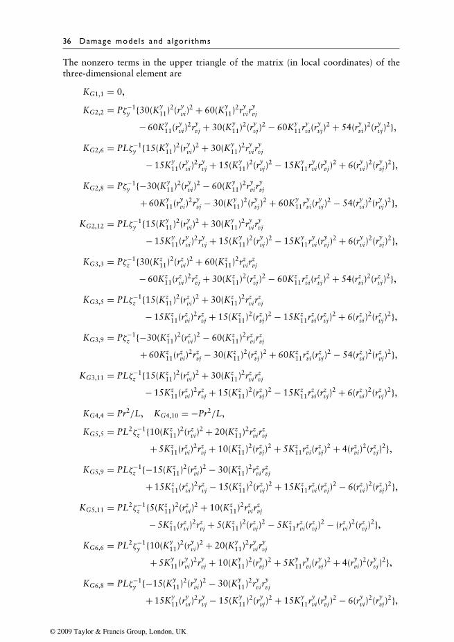
36 Damage mode ls and a lgor i thms
The nonzero terms in the upper triangle of the matrix (in local coordinates) of thethree-dimensional element are
KG1,1 = 0,
KG2,2 = Pζ−1y {30(Ky
11)2(ryvi)
2 + 60(Ky11)2ry
viryvj
− 60Ky11(ry
vi)2ry
vj + 30(Ky11)2(ry
vj)2 − 60Ky
11ryvi(r
yvj)
2 + 54(ryvi)
2(ryvj)
2},KG2,6 = PLζ−1
y {15(Ky11)2(ry
vi)2 + 30(Ky
11)2ryvir
yvj
− 15Ky11(ry
vi)2ry
vj + 15(Ky11)2(ry
vj)2 − 15Ky
11ryvi(r
yvj)
2 + 6(ryvi)
2(ryvj)
2},KG2,8 = Pζ−1
y {−30(Ky11)2(ry
vi)2 − 60(Ky
11)2ryvir
yvj
+ 60Ky11(ry
vi)2ry
vj − 30(Ky11)2(ry
vj)2 + 60Ky
11ryvi(r
yvj)
2 − 54(ryvi)
2(ryvj)
2},KG2,12 = PLζ−1
y {15(Ky11)2(ry
vi)2 + 30(Ky
11)2ryvir
yvj
− 15Ky11(ry
vi)2ry
vj + 15(Ky11)2(ry
vj)2 − 15Ky
11ryvi(r
yvj)
2 + 6(ryvi)
2(ryvj)
2},KG3,3 = Pζ−1
z {30(Kz11)2(rz
vi)2 + 60(Kz
11)2rzvir
zvj
− 60Kz11(rz
vi)2rz
vj + 30(Kz11)2(rz
vj)2 − 60Kz
11rzvi(r
zvj)
2 + 54(rzvi)
2(rzvj)
2},KG3,5 = PLζ−1
z {15(Kz11)2(rz
vi)2 + 30(Kz
11)2rzvir
zvj
− 15Kz11(rz
vi)2rz
vj + 15(Kz11)2(rz
vj)2 − 15Kz
11rzvi(r
zvj)
2 + 6(rzvi)
2(rzvj)
2},KG3,9 = Pζ−1
z {−30(Kz11)2(rz
vi)2 − 60(Kz
11)2rzvir
zvj
+ 60Kz11(rz
vi)2rz
vj − 30(Kz11)2(rz
vj)2 + 60Kz
11rzvi(r
zvj)
2 − 54(rzvi)
2(rzvj)
2},KG3,11 = PLζ−1
z {15(Kz11)2(rz
vi)2 + 30(Kz
11)2rzvir
zvj
− 15Kz11(rz
vi)2rz
vj + 15(Kz11)2(rz
vj)2 − 15Kz
11rzvi(r
zvj)
2 + 6(rzvi)
2(rzvj)
2},KG4,4 = Pr2/L, KG4,10 = −Pr2/L,
KG5,5 = PL2ζ−1z {10(Kz
11)2(rzvi)
2 + 20(Kz11)2rz
virzvj
+ 5Kz11(rz
vi)2rz
vj + 10(Kz11)2(rz
vj)2 + 5Kz
11rzvi(r
zvj)
2 + 4(rzvi)
2(rzvj)
2},KG5,9 = PLζ−1
z {−15(Kz11)2(rz
vi)2 − 30(Kz
11)2rzvir
zvj
+ 15Kz11(rz
vi)2rz
vj − 15(Kz11)2(rz
vj)2 + 15Kz
11rzvi(r
zvj)
2 − 6(rzvi)
2(rzvj)
2},KG5,11 = PL2ζ−1
z {5(Kz11)2(rz
vi)2 + 10(Kz
11)2rzvir
zvj
− 5Kz11(rz
vi)2rz
vj + 5(Kz11)2(rz
vj)2 − 5Kz
11rzvi(r
zvj)
2 − (rzvi)
2(rzvj)
2},KG6,6 = PL2ζ−1
y {10(Ky11)2(ry
vi)2 + 20(Ky
11)2ryvir
yvj
+ 5Ky11(ry
vi)2ry
vj + 10(Ky11)2(ry
vj)2 + 5Ky
11ryvi(r
yvj)
2 + 4(ryvi)
2(ryvj)
2},KG6,8 = PLζ−1
y {−15(Ky11)2(ry
vi)2 − 30(Ky
11)2ryvir
yvj
+ 15Ky11(ry
vi)2ry
vj − 15(Ky11)2(ry
vj)2 + 15Ky
11ryvi(r
yvj)
2 − 6(ryvi)
2(ryvj)
2},
© 2009 Taylor & Francis Group, London, UK
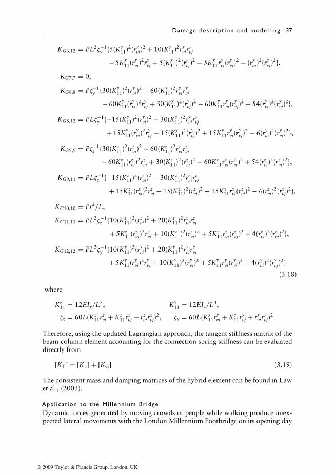
Damage descr ipt ion and mode l l ing 37
KG6,12 = PL2ζ−1y {5(Ky
11)2(ryvi)
2 + 10(Ky11)2ry
viryvj
− 5Ky11(ry
vi)2ry
vj + 5(Ky11)2(ry
vj)2 − 5Ky
11ryvi(r
yvj)
2 − (ryvi)
2(ryvj)
2},KG7,7 = 0,
KG8,8 = Pζ−1y {30(Ky
11)2(ryvi)
2 + 60(Ky11)2ry
viryvj
− 60Ky11(ry
vi)2ry
vj + 30(Ky11)2(ry
vj)2 − 60Ky
11ryvi(r
yvj)
2 + 54(ryvi)
2(ryvj)
2},KG8,12 = PLζ−1
y {−15(Ky11)2(ry
vi)2 − 30(Ky
11)2ryvir
yvj
+ 15Ky11(ry
vi)2ry
vj − 15(Ky11)2(ry
vj)2 + 15Ky
11ryvi(r
yvj)
2 − 6(ryvi)
2(ryvj)
2},KG9,9 = Pζ−1
z {30(Kz11)2(rz
vi)2 + 60(Kz
11)2rzvir
zvj
− 60Kz11(rz
vi)2rz
vj + 30(Kz11)2(rz
vj)2 − 60Kz
11rzvi(r
zvj)
2 + 54(rzvi)
2(rzvj)
2},KG9,11 = PLζ−1
z {−15(Kz11)2(rz
vi)2 − 30(Kz
11)2rzvir
zvj
+ 15Kz11(rz
vi)2rz
vj − 15(Kz11)2(rz
vj)2 + 15Kz
11rzvi(r
zvj)
2 − 6(rzvi)
2(rzvj)
2},KG10,10 = Pr2/L,
KG11,11 = PL2ζ−1z {10(Kz
11)2(rzvi)
2 + 20(Kz11)2rz
virzvj
+ 5Kz11(rz
vi)2rz
vj + 10(Kz11)2(rz
vj)2 + 5Kz
11rzvi(r
zvj)
2 + 4(rzvi)
2(rzvj)
2},KG12,12 = PL2ζ−1
y {10(Ky11)2(ry
vi)2 + 20(Ky
11)2ryvir
yvj
+ 5Ky11(ry
vi)2ry
vj + 10(Ky11)2(ry
vj)2 + 5Ky
11ryvi(r
yvj)
2 + 4(ryvi)
2(ryvj)
2}(3.18)
where
Kz11 = 12EIy/L3, Ky
11 = 12EIz/L3,
ζz = 60L(Kz11rz
vi + Kz11rz
vj + rzvir
zvj)
2, ζy = 60L(Ky11ry
vi + Ky11ry
vj + ryvir
yvj)
2.
Therefore, using the updated Lagrangian approach, the tangent stiffness matrix of thebeam-column element accounting for the connection spring stiffness can be evaluateddirectly from
[KT] = [KL] + [KG] (3.19)
The consistent mass and damping matrices of the hybrid element can be found in Lawet al., (2003).
Appl i ca t ion to the Mi l lenn ium Br idgeDynamic forces generated by moving crowds of people while walking produce unex-pected lateral movements with the London Millennium Footbridge on its opening day
© 2009 Taylor & Francis Group, London, UK

38 Damage mode ls and a lgor i thms
South span
Central span
North span
Edge cable
Figure 3.6 Elevation view of the bridge
Figure 3.7 Deck with 38 hybrid members
(Dallard et al., 2001). The movements took place mainly on the south and centralspans at frequencies corresponding to their first and second lateral modes, which arevery low and between 0.5 and 1.0 Hz. This section presents a vibration mitigationstudy on the footbridge using a bracing member which includes two connecting rodsand a frictional damper, i.e. a slotted, bolted connection element (SBCE).
The bridge structure has three suspended spans. The finite element model is con-structed from the published data of the Millennium Footbridge with a central span of144 m, a south span of 100 m and a north span of 81 m (Dallard et al., 2001). The 4 mwide deck is in segments that are each 16 m long and the steel box sections of the deckare linked together via a tongue and groove movement joint. The segments span over4 m between the edge steel tubes on each side of the bridge. Transverse arms extendingfrom the deck sections clamp onto a 200 mm diameter steel cable at each side of thebridge at 8 m intervals. The cables provide the bridge with both vertical and lateralstiffnesses with a horizontal dead load tension force of approximately 22.5 MN. Thereis only a small sag of cable of 2.3 m over the central span in the tension cable. Thecables are in turn supported by two V-shape steel piers found on a reinforced concretepier foundation. The arrangement of the structure is shown in Figure 3.6.
The hybr id e lementThe finite element model of the structure is referred to by Law et al. (2004b). Thedynamic response of the structure is mitigated by a friction damper installed insidea hybrid-bracing member between corresponding nodal points underneath the bridgedeck as shown in Figure 3.7. The SBCE is modelled as a virtual shear spring betweentwo rod members, and its physical size is assumed infinitely small. Nodes I and J areexternal nodes, and nodes i and j are internal nodes. The SBCE is between nodes iand j. Rods 1 and 2 are between nodes I and i, and between nodes J and j, respectivelyas shown in Figure 3.8.
© 2009 Taylor & Francis Group, London, UK
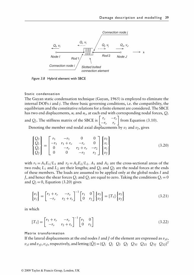
Damage descr ipt ion and mode l l ing 39
x
Slotted boltedconnection element
Connection node i
Connection node j
Node J
QJ, vJQj, vj
Qi, viQI, vI
Node IRod 1
Rod 2
Figure 3.8 Hybrid element with SBCE
Stat i c condensat ionThe Guyan static condensation technique (Guyan, 1965) is employed to eliminate theinternal DOFs i and j. The three basic governing conditions, i.e. the compatibility, theequilibrium and the constitutive relations for a finite element are considered. The SBCEhas two end displacements, ui and uj, at each end with corresponding nodal forces, Qi
and Qj. The stiffness matrix of the SBCE is[
rv −rv
−rv rv
]from Equation (3.10).
Denoting the member end nodal axial displacements by vI and vJ, gives
QI
Qi
Qj
QJ
=
r1 −r1 0 0
−r1 r1 + rv −rv 00 −rv r2 + rv −r2
0 0 −r2 r2
vI
vi
vj
vJ
(3.20)
with r1 = A1E1/L1 and r2 = A2E2/L2. A1 and A2 are the cross-sectional areas of thetwo rods; L1 and L2 are their lengths; and QI and QJ are the nodal forces at the endsof these members. The loads are assumed to be applied only at the global nodes I andJ, and hence the shear forces Qi and Qj are equal to zero. Taking the conditions Qi = 0and Qj = 0, Equation (3.20) gives
{vi
vj
}=[r1 + rv −rv
−rv r2 + rv
]−1 [r1 00 r2
]{vI
vJ
}= [T1]
{vI
vJ
}(3.21)
in which
[T1] =[r1 + rv −rv
−rv r2 + rv
]−1 [r1 00 r2
](3.22)
Matr ix trans format ionIf the lateral displacements at the end nodes I and J of the element are expressed as vyI,vzI and vyJ, vzJ, respectively, and letting {Q} = {Qi Qj QI QJ QYI QZI QYJ QZJ}T
© 2009 Taylor & Francis Group, London, UK
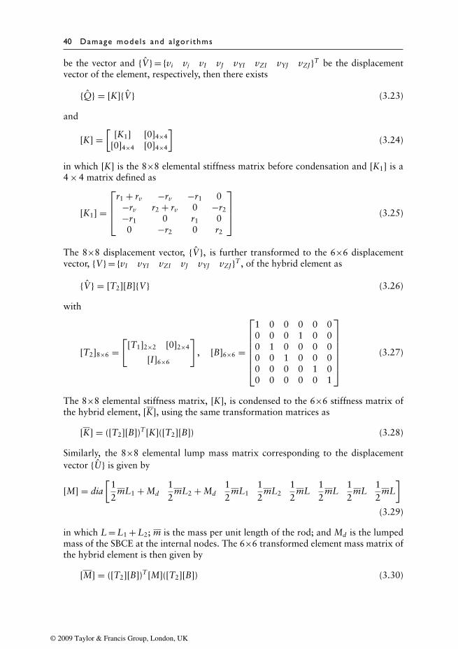
40 Damage mode ls and a lgor i thms
be the vector and {V} = {vi vj vI vJ vYI vZI vYJ vZJ}T be the displacementvector of the element, respectively, then there exists
{Q} = [K]{V} (3.23)
and
[K] =[
[K1] [0]4×4
[0]4×4 [0]4×4
](3.24)
in which [K] is the 8×8 elemental stiffness matrix before condensation and [K1] is a4 × 4 matrix defined as
[K1] =
r1 + rv −rv −r1 0−rv r2 + rv 0 −r2
−r1 0 r1 00 −r2 0 r2
(3.25)
The 8×8 displacement vector, {V}, is further transformed to the 6×6 displacementvector, {V} = {vI vYI vZI vJ vYJ vZJ}T , of the hybrid element as
{V} = [T2][B]{V} (3.26)
with
[T2]8×6 =[
[T1]2×2 [0]2×4
[I]6×6
], [B]6×6 =
1 0 0 0 0 00 0 0 1 0 00 1 0 0 0 00 0 1 0 0 00 0 0 0 1 00 0 0 0 0 1
(3.27)
The 8×8 elemental stiffness matrix, [K], is condensed to the 6×6 stiffness matrix ofthe hybrid element, [K], using the same transformation matrices as
[K] = ([T2][B])T [K]([T2][B]) (3.28)
Similarly, the 8×8 elemental lump mass matrix corresponding to the displacementvector {U} is given by
[M] = dia[
12
mL1 + Md12
mL2 + Md12
mL112
mL212
mL12
mL12
mL12
mL]
(3.29)
in which L = L1 + L2; m is the mass per unit length of the rod; and Md is the lumpedmass of the SBCE at the internal nodes. The 6×6 transformed element mass matrix ofthe hybrid element is then given by
[M] = ([T2][B])T [M]([T2][B]) (3.30)
© 2009 Taylor & Francis Group, London, UK
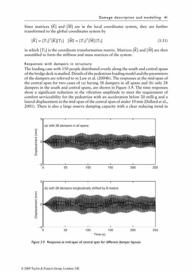
Damage descr ipt ion and mode l l ing 41
Since matrices [K] and [M] are in the local coordinates system, they are furthertransformed to the global coordinates system by
[K] = [T3]T [K][T3] [M] = [T3]T [M] [T3] (3.31)
in which [T3] is the coordinate transformation matrix. Matrices [K] and [M] are thenassembled to form the stiffness and mass matrices of the system.
Responses wi th dampers in s tructureThe loading case with 150 people distributed evenly along the south and central spansof the bridge deck is studied. Details of the pedestrian loading model and the parametersof the dampers are referred to in Law et al. (2004b). The responses at the mid-span ofthe central span for two cases of (a) having 38 dampers in all spans and (b) only 28dampers in the south and central spans, are shown in Figure 3.9. The time responsesshow a significant reduction in the vibration amplitude to meet the requirement ofcomfort serviceability for the pedestrian with an acceleration below 20 milli-g and alateral displacement at the mid-span of the central span of under 10 mm (Dallard et al.,2001). There is also a large reserve damping capacity with a clear reducing trend in
(a) with 38 dampers in all spans
5
0
0 50 100 150 200 250�5
Dis
plac
emen
t (m
m)
(b) with 28 dampers longitudinally shifted by 8 meters
5
0
0 50 100 150Time (s)
200 250�5
Dis
plac
emen
t (m
m)
Figure 3.9 Response at mid-span of central span for different damper layouts
© 2009 Taylor & Francis Group, London, UK
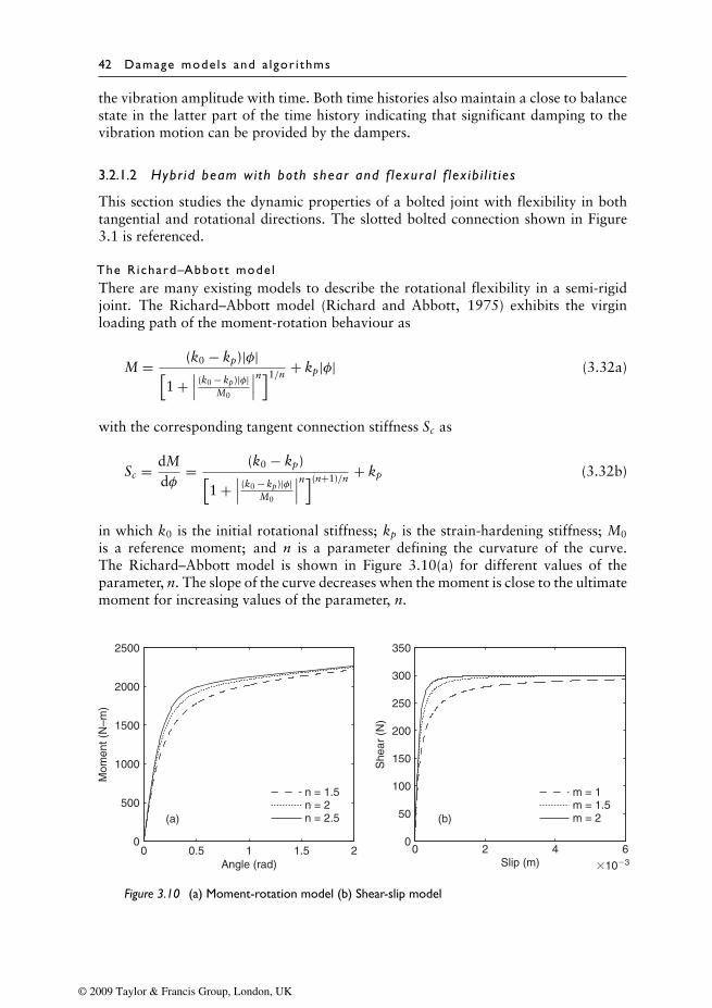
42 Damage mode ls and a lgor i thms
the vibration amplitude with time. Both time histories also maintain a close to balancestate in the latter part of the time history indicating that significant damping to thevibration motion can be provided by the dampers.
3.2.1.2 Hybr id beam with both shear and f lexura l f lex ib i l i t i es
This section studies the dynamic properties of a bolted joint with flexibility in bothtangential and rotational directions. The slotted bolted connection shown in Figure3.1 is referenced.
The Richard–Abbott mode lThere are many existing models to describe the rotational flexibility in a semi-rigidjoint. The Richard–Abbott model (Richard and Abbott, 1975) exhibits the virginloading path of the moment-rotation behaviour as
M = (k0 − kp)|φ|[1 +
∣∣∣ (k0 − kp)|φ|M0
∣∣∣n]1/n + kp|φ| (3.32a)
with the corresponding tangent connection stiffness Sc as
Sc = dMdφ
= (k0 − kp)[1 +
∣∣∣ (k0 − kp)|φ|M0
∣∣∣n](n+1)/n + kp (3.32b)
in which k0 is the initial rotational stiffness; kp is the strain-hardening stiffness; M0
is a reference moment; and n is a parameter defining the curvature of the curve.The Richard–Abbott model is shown in Figure 3.10(a) for different values of theparameter, n. The slope of the curve decreases when the moment is close to the ultimatemoment for increasing values of the parameter, n.
0 2 4 6
�10�3
0
50
100
150
200
250
300
350
Slip (m)
She
ar (
N)
m = 1m = 1.5m = 2
0 0.5 1 1.5 20
500
1000
1500
2000
2500
Angle (rad)
Mom
ent (
N–m
)
n = 1.5n = 2n = 2.5 (b)(a)
Figure 3.10 (a) Moment-rotation model (b) Shear-slip model
© 2009 Taylor & Francis Group, London, UK
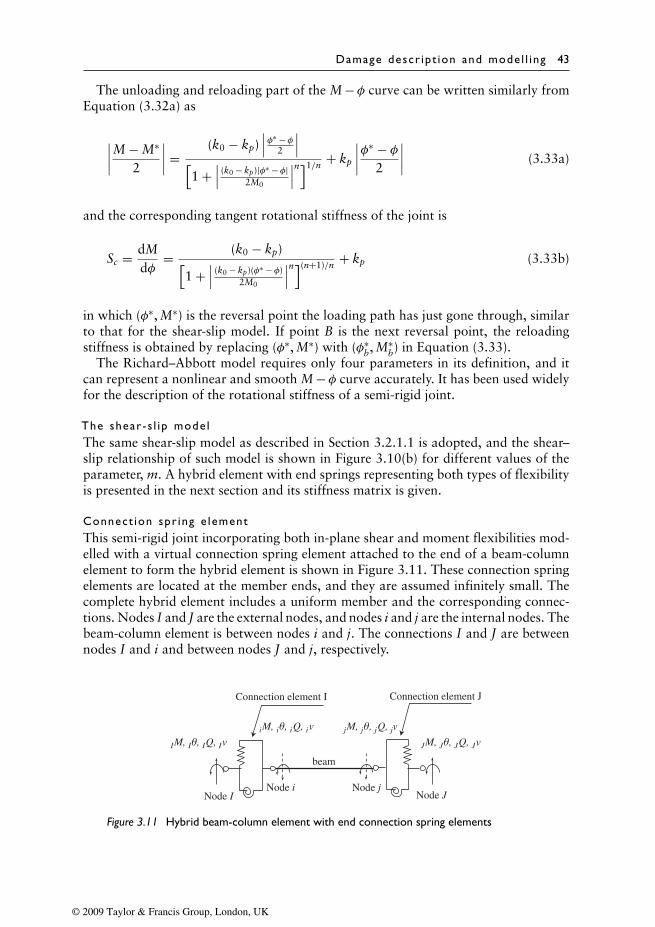
Damage descr ipt ion and mode l l ing 43
The unloading and reloading part of the M −φ curve can be written similarly fromEquation (3.32a) as
∣∣∣∣M − M∗
2
∣∣∣∣ =(k0 − kp)
∣∣∣φ∗ −φ2
∣∣∣[1 +
∣∣∣ (k0 − kp)|φ∗ −φ|2M0
∣∣∣n]1/n + kp
∣∣∣∣φ∗ − φ2
∣∣∣∣ (3.33a)
and the corresponding tangent rotational stiffness of the joint is
Sc = dMdφ
= (k0 − kp)[1 +
∣∣∣ (k0 − kp)(φ∗ −φ)2M0
∣∣∣n](n+1)/n + kp (3.33b)
in which (φ∗, M∗) is the reversal point the loading path has just gone through, similarto that for the shear-slip model. If point B is the next reversal point, the reloadingstiffness is obtained by replacing (φ∗, M∗) with (φ∗
b, M∗b) in Equation (3.33).
The Richard–Abbott model requires only four parameters in its definition, and itcan represent a nonlinear and smooth M − φ curve accurately. It has been used widelyfor the description of the rotational stiffness of a semi-rigid joint.
The shear-s l ip mode lThe same shear-slip model as described in Section 3.2.1.1 is adopted, and the shear–slip relationship of such model is shown in Figure 3.10(b) for different values of theparameter, m. A hybrid element with end springs representing both types of flexibilityis presented in the next section and its stiffness matrix is given.
Connect ion spr ing e lementThis semi-rigid joint incorporating both in-plane shear and moment flexibilities mod-elled with a virtual connection spring element attached to the end of a beam-columnelement to form the hybrid element is shown in Figure 3.11. These connection springelements are located at the member ends, and they are assumed infinitely small. Thecomplete hybrid element includes a uniform member and the corresponding connec-tions. Nodes I and J are the external nodes, and nodes i and j are the internal nodes. Thebeam-column element is between nodes i and j. The connections I and J are betweennodes I and i and between nodes J and j, respectively.
beam
Node INode i Node j
Node J
Connection element JConnection element I
IM, Iθ, IQ, Iv JM, Jθ, JQ, JvjM, jθ, jQ, jviM, iθ, iQ, iv
Figure 3.11 Hybrid beam-column element with end connection spring elements
© 2009 Taylor & Francis Group, London, UK
44 Damage mode ls and a lgor i thms
In the derivation of the spring stiffness matrix, the three basic governing conditions,i.e. the compatibility, the equilibrium and the constitutive relations for an element, areconsidered. Considering a spring with stiffnesses Sc and rv; two end displacements, Ivand iv; and two rotations, Iθ and iθ, on either side of the spring, the corresponding lat-eral shear forces, IQ and iQ, and corresponding moments IM and iM, the equilibriumconditions require
IQ + iQ = 0, IM + iM = 0 (3.34)
Assuming that v is the relative shear displacement between the joint interfaces, andθ is the connection rotation angle, the compatibility conditions require
v = Iv − iv, θ = Iθ − iθ (3.35)
The constitutive relationships of the shearing and rotational actions are
rv = IQv
= iQv
, Sc = IMθ
= iMθ
(3.36)
Substituting Equation (3.34) into Equation (3.36), gives{IQiQ
}=[
rv −rv
−rv rv
]{Iviv
},
{IMiM
}=[
Sc −Sc
−Sc Sc
]{Iθ
iθ
}(3.37)
Therefore, the in-plane stiffness matrix of the connection element is given by:rv 0 −rv 00 Sc 0 −Sc
−rv 0 −rv 00 Sc 0 Sc
(3.38)
The shape funct ionBy using the cubic Hermitian function, the lateral deflection, v, in the y-direction at alocation x along the centre-line of a straight element can be written as
v = a0 + a1x + a2x2 + a3x3 (3.39)
in which (aj, j = 0, 1, 2, 3) are coefficients. Denoting the beam end rotations by θi andθj, and the beam end lateral deflections by vi and vj at the end nodes i and j of theelement respectively, gives the following boundary conditions
v = vi,dvdx
= θi, at x = 0,
v = vj,dvdx
= θj, at x = L, (3.40)
in which L is the length of the element.
© 2009 Taylor & Francis Group, London, UK
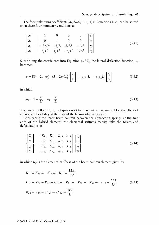
Damage descr ipt ion and mode l l ing 45
The four unknowns coefficients (aj, j = 0, 1, 2, 3) in Equation (3.39) can be solvedfrom these four boundary conditions as
a0
a1
a2
a3
=
1 0 0 0
0 1 0 0
−3/L2 −2/L 3/L2 −1/L
2/L3 1/L2 −2/L3 1/L2
vi
θi
vj
θj
(3.41)
Substituting the coefficients into Equation (3.39), the lateral deflection function, v,becomes
v = [(3 − 2ρ1)ρ21 (3 − 2ρ2)ρ2
2]
[vi
vj
]+ [ρ2
1ρ2L −ρ1ρ22L]
[θi
θj
](3.42)
in which
ρ1 = 1 − xL
, ρ2 = xL. (3.43)
The lateral deflection, v, in Equation (3.42) has not yet accounted for the effect ofconnection flexibility at the ends of the beam-column element.
Considering the inner beam-column between the connection springs at the twoends of the hybrid element, the elemental stiffness matrix links the forces anddeformations as
Qi
Mi
Qj
Mj
=
K11 K12 K13 K14
K21 K22 K23 K24
K31 K32 K33 K34
K41 K42 K43 K44
vi
θi
vj
θj
(3.44)
in which Kij is the elemental stiffness of the beam-column element given by
K11 = K33 = −K13 = −K31 = 12EIL3
K12 = K21 = K14 = K41 = −K23 = −K32 = −K34 = −K43 = 6EIL2
(3.45)
K22 = K44 = 2K24 = 2K42 = 4EIL
© 2009 Taylor & Francis Group, London, UK

46 Damage mode ls and a lgor i thms
The elemental stiffness matrix for the complete hybrid element, with the connectionsprings at two ends of the beam-column element, can be written as
Qi
Mi
Qj
Mj
QI
MI
QJ
MJ
=
rvi + K11 K12 K13 K14 −rvi 0 0 0K21 Sci + K22 K23 K24 0 −Sci 0 0K31 K32 rvj + K33 K34 0 0 −rvj 0K41 K42 K43 Scj + K44 0 0 0 −Scj
−rvi 0 0 0 rvi 0 0 00 −Sci 0 0 0 Sci 0 00 0 −rvj 0 0 0 rvj 00 0 0 −Scj 0 0 0 Scj
vi
θivj
θjvI
θIvJ
θJ
(3.46)
The loads are assumed to be applied only at the global nodes I and J, and hence theshear forces, Qi and Qj, and moments, Mi and Mj, are equal to zero. Thus,
vi
θivj
θj
=
rvi + K11 K12 K13 K14
K21 Sci + K22 K23 K24
K31 K32 rvj + K33 K34
K41 K42 K43 Scj + K44
−1
rvi 0 0 00 Sci 0 00 0 rvj 00 0 0 Scj
vI
θIvJ
θJ
(3.47)
The internal DOFs are eliminated by substituting Equation (3.47) into Equation(3.46), thus the relationship between the external nodal force and nodal displace-ments/rotations of the element can be obtained.
In the assembling of the elemental stiffness matrix of a structure, the above matrixis rewritten in the global coordinate system for geometrical compatibility. SubstitutingEquation (3.47) into Equation (3.42) and transforming the external nodal deforma-tions, vI, θI and vJ, θJ, about the local axis at the ends of the element to the global nodaldeformations vi, θi and vj, θj, the displacement function v can finally be written as
v = [(3 − 2ρ1)ρ21 ρ2
1ρ2L (3 − 2ρ2)ρ22 −ρ1ρ
22L]
×
rvi + K11 K12 K13 K14
K21 Sci + K22 K23 K24
K31 K32 rvj + K33 K34
K41 K42 K43 Scj + K44
−1
rvi 0 0 00 Sci 0 00 0 rvj 00 0 0 Scj
× [T]
vi
θivj
θj
(3.48)
in which [T] is the coordinate transformation matrix.
3.2.2 Decomposit ion of system matrices
A number of new finite element model updating methodologies have been proposed andapplied to structural engineering for solving the inverse problem of model updatingor damage assessment (Mottershead and Friswell, 1993). There are two importantissues in the use of the model updating methods: (a) the selection strategy for the
© 2009 Taylor & Francis Group, London, UK
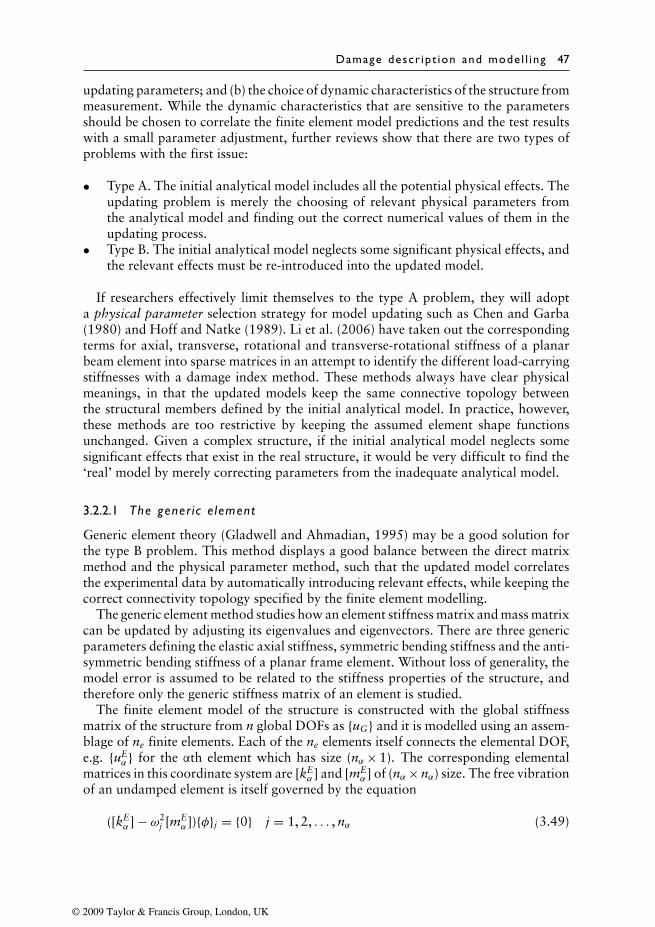
Damage descr ipt ion and mode l l ing 47
updating parameters; and (b) the choice of dynamic characteristics of the structure frommeasurement. While the dynamic characteristics that are sensitive to the parametersshould be chosen to correlate the finite element model predictions and the test resultswith a small parameter adjustment, further reviews show that there are two types ofproblems with the first issue:
• Type A. The initial analytical model includes all the potential physical effects. Theupdating problem is merely the choosing of relevant physical parameters fromthe analytical model and finding out the correct numerical values of them in theupdating process.
• Type B. The initial analytical model neglects some significant physical effects, andthe relevant effects must be re-introduced into the updated model.
If researchers effectively limit themselves to the type A problem, they will adopta physical parameter selection strategy for model updating such as Chen and Garba(1980) and Hoff and Natke (1989). Li et al. (2006) have taken out the correspondingterms for axial, transverse, rotational and transverse-rotational stiffness of a planarbeam element into sparse matrices in an attempt to identify the different load-carryingstiffnesses with a damage index method. These methods always have clear physicalmeanings, in that the updated models keep the same connective topology betweenthe structural members defined by the initial analytical model. In practice, however,these methods are too restrictive by keeping the assumed element shape functionsunchanged. Given a complex structure, if the initial analytical model neglects somesignificant effects that exist in the real structure, it would be very difficult to find the‘real’ model by merely correcting parameters from the inadequate analytical model.
3.2.2.1 The gener ic e lement
Generic element theory (Gladwell and Ahmadian, 1995) may be a good solution forthe type B problem. This method displays a good balance between the direct matrixmethod and the physical parameter method, such that the updated model correlatesthe experimental data by automatically introducing relevant effects, while keeping thecorrect connectivity topology specified by the finite element modelling.
The generic element method studies how an element stiffness matrix and mass matrixcan be updated by adjusting its eigenvalues and eigenvectors. There are three genericparameters defining the elastic axial stiffness, symmetric bending stiffness and the anti-symmetric bending stiffness of a planar frame element. Without loss of generality, themodel error is assumed to be related to the stiffness properties of the structure, andtherefore only the generic stiffness matrix of an element is studied.
The finite element model of the structure is constructed with the global stiffnessmatrix of the structure from n global DOFs as {uG} and it is modelled using an assem-blage of ne finite elements. Each of the ne elements itself connects the elemental DOF,e.g. {uE
α } for the αth element which has size (nα× 1). The corresponding elementalmatrices in this coordinate system are [kE
α ] and [mEα ] of (nα× nα) size. The free vibration
of an undamped element is itself governed by the equation
([kEα ] − ω2
j [mEα ]){φ}j = {0} j = 1, 2, . . . , nα (3.49)
© 2009 Taylor & Francis Group, London, UK
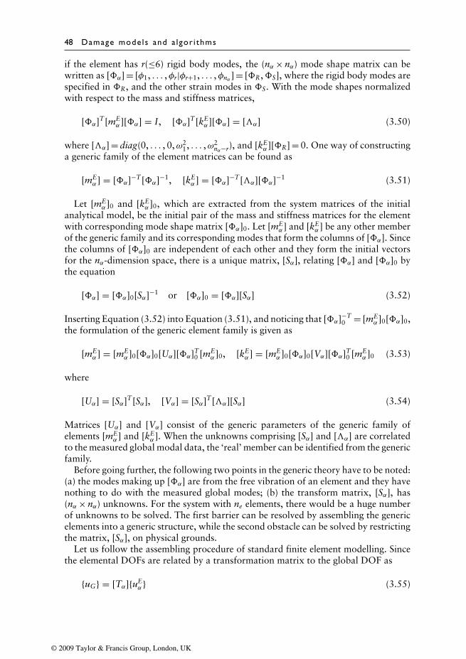
48 Damage mode ls and a lgor i thms
if the element has r(≤6) rigid body modes, the (nα× nα) mode shape matrix can bewritten as [�α] = [φ1, . . . ,φr|φr+1, . . . ,φnα ] = [�R,�S], where the rigid body modes arespecified in �R, and the other strain modes in �S. With the mode shapes normalizedwith respect to the mass and stiffness matrices,
[�α]T [mEα ][�α] = I, [�α]T [kE
α ][�α] = [�α] (3.50)
where [�α] = diag(0, . . . , 0,ω21, . . . ,ω2
nα−r), and [kEα ][�R] = 0. One way of constructing
a generic family of the element matrices can be found as
[mEα ] = [�α]−T [�α]−1, [kE
α ] = [�α]−T [�α][�α]−1 (3.51)
Let [mEα ]0 and [kE
α ]0, which are extracted from the system matrices of the initialanalytical model, be the initial pair of the mass and stiffness matrices for the elementwith corresponding mode shape matrix [�α]0. Let [mE
α ] and [kEα ] be any other member
of the generic family and its corresponding modes that form the columns of [�α]. Sincethe columns of [�α]0 are independent of each other and they form the initial vectorsfor the nα-dimension space, there is a unique matrix, [Sα], relating [�α] and [�α]0 bythe equation
[�α] = [�α]0[Sα]−1 or [�α]0 = [�α][Sα] (3.52)
Inserting Equation (3.52) into Equation (3.51), and noticing that [�α]−T0 = [mE
α ]0[�α]0,the formulation of the generic element family is given as
[mEα ] = [mE
α ]0[�α]0[Uα][�α]T0 [mE
α ]0, [kEα ] = [mE
α ]0[�α]0[Vα][�α]T0 [mE
α ]0 (3.53)
where
[Uα] = [Sα]T [Sα], [Vα] = [Sα]T [�α][Sα] (3.54)
Matrices [Uα] and [Vα] consist of the generic parameters of the generic family ofelements [mE
α ] and [kEα ]. When the unknowns comprising [Sα] and [�α] are correlated
to the measured global modal data, the ‘real’ member can be identified from the genericfamily.
Before going further, the following two points in the generic theory have to be noted:(a) the modes making up [�α] are from the free vibration of an element and they havenothing to do with the measured global modes; (b) the transform matrix, [Sα], has(nα× nα) unknowns. For the system with ne elements, there would be a huge numberof unknowns to be solved. The first barrier can be resolved by assembling the genericelements into a generic structure, while the second obstacle can be solved by restrictingthe matrix, [Sα], on physical grounds.
Let us follow the assembling procedure of standard finite element modelling. Sincethe elemental DOFs are related by a transformation matrix to the global DOF as
{uG} = [Tα]{uEα } (3.55)
© 2009 Taylor & Francis Group, London, UK
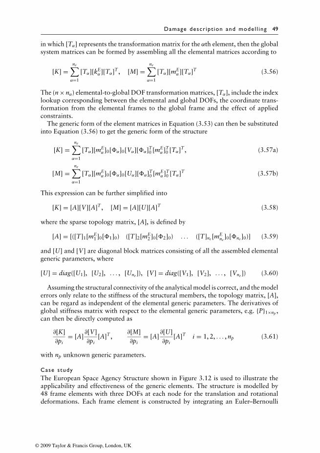
Damage descr ipt ion and mode l l ing 49
in which [Tα] represents the transformation matrix for the αth element, then the globalsystem matrices can be formed by assembling all the elemental matrices according to
[K] =ne∑α=1
[Tα][kEα ][Tα]T , [M] =
ne∑α=1
[Tα][mEα ][Tα]T (3.56)
The (n × nα) elemental-to-global DOF transformation matrices, [Tα], include the indexlookup corresponding between the elemental and global DOFs, the coordinate trans-formation from the elemental frames to the global frame and the effect of appliedconstraints.
The generic form of the element matrices in Equation (3.53) can then be substitutedinto Equation (3.56) to get the generic form of the structure
[K] =ne∑α=1
[Tα][mEα ]0[�α]0[Vα][�α]T
0 [mEα ]T
0 [Tα]T , (3.57a)
[M] =ne∑α=1
[Tα][mEα ]0[�α]0[Uα][�α]T
0 [mEα ]T
0 [Tα]T (3.57b)
This expression can be further simplified into
[K] = [A][V][A]T , [M] = [A][U][A]T (3.58)
where the sparse topology matrix, [A], is defined by
[A] = [([T]1[mE1 ]0[�1]0) ([T]2[mE
2 ]0[�2]0) . . . ([T]ne [mEne
]0[�ne ]0)] (3.59)
and [U] and [V] are diagonal block matrices consisting of all the assembled elementalgeneric parameters, where
[U] = diag([U1], [U2], . . . , [Une ]), [V] = diag([V1], [V2], . . . , [Vne ]) (3.60)
Assuming the structural connectivity of the analytical model is correct, and the modelerrors only relate to the stiffness of the structural members, the topology matrix, [A],can be regard as independent of the elemental generic parameters. The derivatives ofglobal stiffness matrix with respect to the elemental generic parameters, e.g. {P}1×np ,can then be directly computed as
∂[K]∂pi
= [A]∂[V]∂pi
[A]T ,∂[M]∂pi
= [A]∂[U]∂pi
[A]T i = 1, 2, . . . , np (3.61)
with np unknown generic parameters.
Case studyThe European Space Agency Structure shown in Figure 3.12 is used to illustrate theapplicability and effectiveness of the generic elements. The structure is modelled by48 frame elements with three DOFs at each node for the translation and rotationaldeformations. Each frame element is constructed by integrating an Euler–Bernoulli
© 2009 Taylor & Francis Group, London, UK
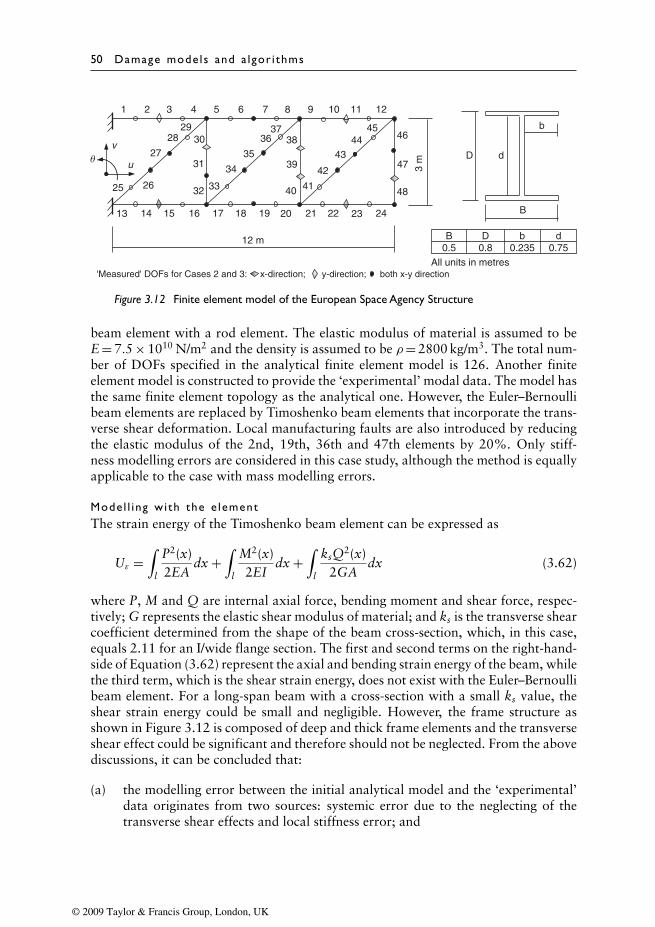
50 Damage mode ls and a lgor i thms
3 m
vθ u
12 m
1 2 3 4 5 6 7 8 9 10 11 12
13 14 15 16 17 18 19 20 21 22 23 24
46
47
4825 26
27
28 29
30
31
32 33
34
35
36 37
40
39
38
41
42
43
4445
B
D d
b
All units in metres
B D b d0.5 0.8 0.235 0.75
'Measured' DOFs for Cases 2 and 3: x-direction; y-direction; both x-y direction
Figure 3.12 Finite element model of the European Space Agency Structure
beam element with a rod element. The elastic modulus of material is assumed to beE = 7.5 × 10¹⁰ N/m2 and the density is assumed to be ρ= 2800 kg/m3. The total num-ber of DOFs specified in the analytical finite element model is 126. Another finiteelement model is constructed to provide the ‘experimental’ modal data. The model hasthe same finite element topology as the analytical one. However, the Euler–Bernoullibeam elements are replaced by Timoshenko beam elements that incorporate the trans-verse shear deformation. Local manufacturing faults are also introduced by reducingthe elastic modulus of the 2nd, 19th, 36th and 47th elements by 20%. Only stiff-ness modelling errors are considered in this case study, although the method is equallyapplicable to the case with mass modelling errors.
Model l ing wi th the e lementThe strain energy of the Timoshenko beam element can be expressed as
Uε =∫
l
P2(x)2EA
dx +∫
l
M2(x)2EI
dx +∫
l
ksQ2(x)2GA
dx (3.62)
where P, M and Q are internal axial force, bending moment and shear force, respec-tively; G represents the elastic shear modulus of material; and ks is the transverse shearcoefficient determined from the shape of the beam cross-section, which, in this case,equals 2.11 for an I/wide flange section. The first and second terms on the right-hand-side of Equation (3.62) represent the axial and bending strain energy of the beam, whilethe third term, which is the shear strain energy, does not exist with the Euler–Bernoullibeam element. For a long-span beam with a cross-section with a small ks value, theshear strain energy could be small and negligible. However, the frame structure asshown in Figure 3.12 is composed of deep and thick frame elements and the transverseshear effect could be significant and therefore should not be neglected. From the abovediscussions, it can be concluded that:
(a) the modelling error between the initial analytical model and the ‘experimental’data originates from two sources: systemic error due to the neglecting of thetransverse shear effects and local stiffness error; and
© 2009 Taylor & Francis Group, London, UK
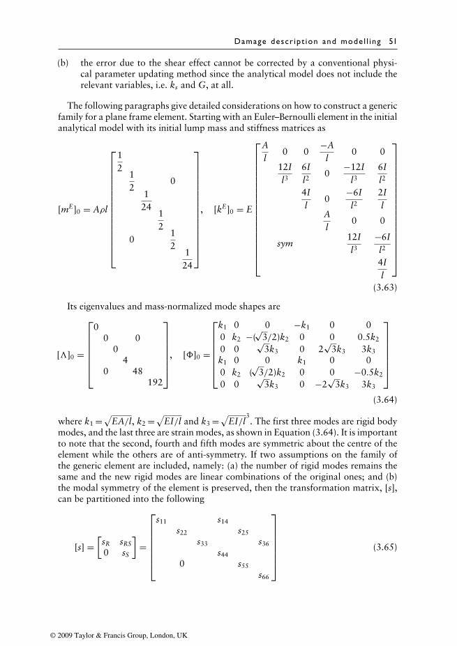
Damage descr ipt ion and mode l l ing 51
(b) the error due to the shear effect cannot be corrected by a conventional physi-cal parameter updating method since the analytical model does not include therelevant variables, i.e. ks and G, at all.
The following paragraphs give detailed considerations on how to construct a genericfamily for a plane frame element. Starting with an Euler–Bernoulli element in the initialanalytical model with its initial lump mass and stiffness matrices as
[mE]0 = Aρl
12
12
0124
12
012
124
, [kE]0 = E
Al
0 0−A
l0 0
12Il3
6Il2
0−12I
l3
6Il2
4Il
0−6Il2
2Il
Al
0 0
sym12Il3
−6Il2
4Il
(3.63)
Its eigenvalues and mass-normalized mode shapes are
[�]0 =
0
0 00
40 48
192
, [�]0 =
k1 0 0 −k1 0 00 k2 −(
√3/2)k2 0 0 0.5k2
0 0√
3k3 0 2√
3k3 3k3
k1 0 0 k1 0 00 k2 (
√3/2)k2 0 0 −0.5k2
0 0√
3k3 0 −2√
3k3 3k3
(3.64)
where k1 =√EA/l, k2 =√
EI/l and k3 =√EI/l
3. The first three modes are rigid body
modes, and the last three are strain modes, as shown in Equation (3.64). It is importantto note that the second, fourth and fifth modes are symmetric about the centre of theelement while the others are of anti-symmetry. If two assumptions on the family ofthe generic element are included, namely: (a) the number of rigid modes remains thesame and the new rigid modes are linear combinations of the original ones; and (b)the modal symmetry of the element is preserved, then the transformation matrix, [s],can be partitioned into the following
[s] =[sR sRS
0 sS
]=
s11 s14
s22 s25
s33 s36
s44
0 s55
s66
(3.65)
© 2009 Taylor & Francis Group, London, UK

52 Damage mode ls and a lgor i thms
This then leads to a diagonal matrix, [V], in Equation (3.53), such that the stiffnessmatrix of the generic element family can be expressed as (Law et al., 2001a)
[kE] = [mE]0
−k1 0 00 0 0.5k2
0 2√
3k3 3k3
k1 0 00 0 −0.5k2
0 −2√
3k3 3k3
v1 0
v2
0 v3
×−k1 0 0 k1 0 0
0 0 2√
3k3 0 0 −2√
3k3
0 0.5k2 3k3 0 −0.5k2 3k3
[mE]0 (3.66)
where v1 =ω21s2
44, v2 =ω22s2
55 and v3 =ω23s2
66; and ωi is the ith elastic circular frequency.There are only three generic parameters to define the stiffness matrix for each element.
Since the transfer matrix, [s]0, corresponding to the initial finite element modelis a unity matrix, the generic parameters take the initial values of v1 = 4, v2 = 48and v3 = 192. It is noted that v1, v2 and v3 correspond to the elastic axial mode,symmetric bending mode and the anti-symmetric bending mode, respectively. Whenthese parameters take different values, the stiffness matrix represents elements withdifferent stiffness properties. For example, when only one generic parameter, s66, takesthe form as s66 =√
1/(1 + b),
v3 = 192/(1 + b) (3.67)
in which b = 12EIks/GAl2. Substituting v3 into Equation (3.66) gives the familiarstiffness matrix of a Timoshenko beam element
[kE] = E1 + b
A(1 + b)l
0 0−A(1 + b)
l0 0
12Il3
6Il2
0−12I
l3
6Il2
(4 + b)Il
0−6Il2
(2 − b)Il
A(1 + b)l
0 0
sym12Il3
−6Il2
(4 + b)Il
(3.68)
It is noted that taking all the three generic parameters as variables gives us a verylarge family of generic elements that can include many types of modelling errors andunknown effects.
3.2.2.2 The e igen-decompos i t ion
A uniform stiffness (or mass) reduction is widely adopted by researchers to model localdamage sites. In practice, however, the damage may be of different patterns, which
© 2009 Taylor & Francis Group, London, UK
Damage descr ipt ion and mode l l ing 53
affect the system dynamic properties differently and it cannot be modelled as a uniformchange in the stiffness or mass matrix without much error. To describe the damage ofall possible patterns with one set of indicators, a more generalized parameter set, calledthe elemental eigen-parameters, is formulated.
The elemental matrices of a frame element are decomposed into their eigenvalueand eigenvector matrices. The eigenvalues represent physically the stiffnesses of theelement corresponding to its different deformed shapes. The different eigenvalues givea detailed description of the different load-carrying resistances of the structure.
The global stiffness matrix of a structure, consisting of n global DOFs, {uG}, can bemodelled using an assembly of ne finite elements. The elemental local DOFs are relatedto the global DOFs by
{uG} =ne∑α=1
[T]α{uE}α (3.69)
in which [T]α is the transformation matrix for the αth element. The global systemmatrices are assembled as
[K] =ne∑α=1
[T]α[kE]α[T]Tα , [M] =
ne∑α=1
[T]α[mE]α[T]Tα (3.70)
It is important to note that Equation (3.70) is not a minimum-rank definition ofthe structural disassembly problem, because the elemental matrices [kE]α and [mE]αare always rank deficient. Although [kE]α is an (nα× nα) symmetric matrix with(nα× (nα+ 1)/2) unknown entries, only a few of them are actually independent. Con-sider as an example, a linear spring element connecting two nodes, each of whichincludes three displacement {u, v, w} DOFs. There are potentially 21 unknownentries in this (6×6) element stiffness matrix. However, the rank of the elementalstiffness matrix is one, as there is only one axial stiffness of the spring in the matrix.
The rank deficient elemental matrices can be decomposed into their static eigenvaluesand eigenvectors (Doebling, 1995; Doebling et al., 1998a) such that
[kE]α = [η]α[pk]α[η]Tα , [mE]α = [µ]α[pm]α[µ]T
α (3.71)
where [pk]α and [pm]α are the corresponding diagonal matrices of nonzero static eigen-values. If the ranks of the stiffness and mass matrices for the αth element are rα andτα, respectively, then [η]α is an (nα× rα) eigenvector matrix of the elemental stiffnessmatrix and [µ]α is an (nα× τα) eigenvector matrix of the mass matrix. Physically, thecolumns of matrix [η]α are the distinct and statically equilibrated deformation shapesof the element which have nonzero strain energy, while those of matrix [µ]α are rigiddisplacements related to the kinetic energy. Both these matrices can be normalized as
[η]Tα [η]α = [I]rα , [µ]T
α [µ]α = [I]τα (3.72)
© 2009 Taylor & Francis Group, London, UK
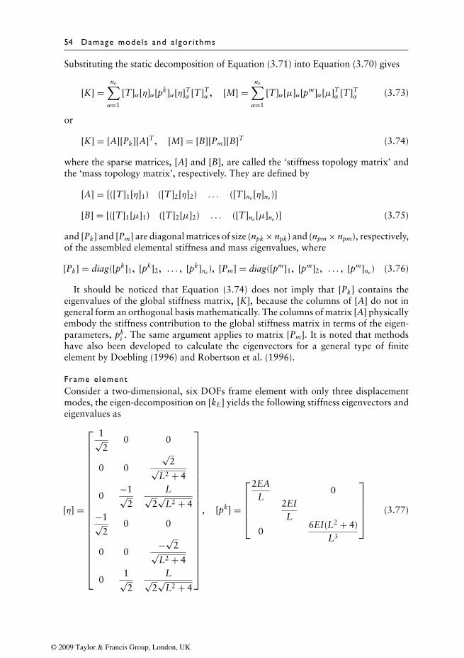
54 Damage mode ls and a lgor i thms
Substituting the static decomposition of Equation (3.71) into Equation (3.70) gives
[K] =ne∑α=1
[T]α[η]α[pk]α[η]Tα [T]T
α , [M] =ne∑α=1
[T]α[µ]α[pm]α[µ]Tα [T]T
α (3.73)
or
[K] = [A][Pk][A]T , [M] = [B][Pm][B]T (3.74)
where the sparse matrices, [A] and [B], are called the ‘stiffness topology matrix’ andthe ‘mass topology matrix’, respectively. They are defined by
[A] = [([T]1[η]1) ([T]2[η]2) . . . ([T]ne [η]ne )]
[B] = [([T]1[µ]1) ([T]2[µ]2) . . . ([T]ne [µ]ne )] (3.75)
and [Pk] and [Pm] are diagonal matrices of size (npk × npk) and (npm × npm), respectively,of the assembled elemental stiffness and mass eigenvalues, where
[Pk] = diag([pk]1, [pk]2, . . . , [pk]ne ), [Pm] = diag([pm]1, [pm]2, . . . , [pm]ne ) (3.76)
It should be noticed that Equation (3.74) does not imply that [Pk] contains theeigenvalues of the global stiffness matrix, [K], because the columns of [A] do not ingeneral form an orthogonal basis mathematically. The columns of matrix [A] physicallyembody the stiffness contribution to the global stiffness matrix in terms of the eigen-parameters, pk
i . The same argument applies to matrix [Pm]. It is noted that methodshave also been developed to calculate the eigenvectors for a general type of finiteelement by Doebling (1996) and Robertson et al. (1996).
Frame e lementConsider a two-dimensional, six DOFs frame element with only three displacementmodes, the eigen-decomposition on [kE] yields the following stiffness eigenvectors andeigenvalues as
[η] =
1√2
0 0
0 0
√2√
L2 + 4
0−1√
2
L√2√
L2 + 4−1√
20 0
0 0−√
2√L2 + 4
01√2
L√2√
L2 + 4
, [pk] =
2EA
L0
2EIL
06EI(L2 + 4)
L3
(3.77)
© 2009 Taylor & Francis Group, London, UK
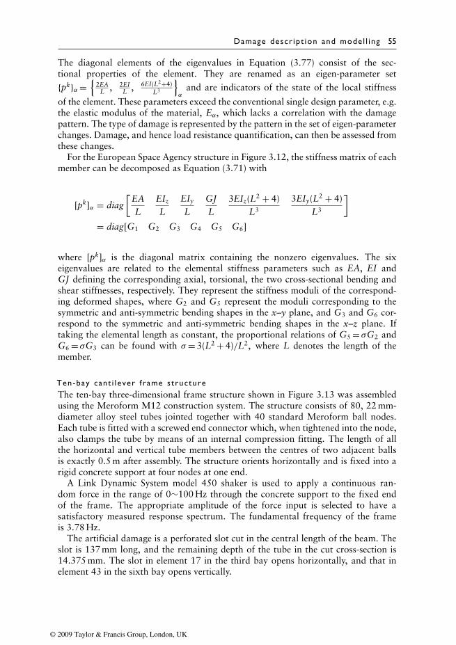
Damage descr ipt ion and mode l l ing 55
The diagonal elements of the eigenvalues in Equation (3.77) consist of the sec-tional properties of the element. They are renamed as an eigen-parameter set
{pk}α={
2EAL , 2EI
L , 6EI(L2+4)L3
}α
and are indicators of the state of the local stiffness
of the element. These parameters exceed the conventional single design parameter, e.g.the elastic modulus of the material, Eα, which lacks a correlation with the damagepattern. The type of damage is represented by the pattern in the set of eigen-parameterchanges. Damage, and hence load resistance quantification, can then be assessed fromthese changes.
For the European Space Agency structure in Figure 3.12, the stiffness matrix of eachmember can be decomposed as Equation (3.71) with
[pk]α = diag[
EAL
EIz
LEIy
LGJL
3EIz(L2 + 4)L3
3EIy(L2 + 4)L3
]= diag[G1 G2 G3 G4 G5 G6]
where [pk]α is the diagonal matrix containing the nonzero eigenvalues. The sixeigenvalues are related to the elemental stiffness parameters such as EA, EI andGJ defining the corresponding axial, torsional, the two cross-sectional bending andshear stiffnesses, respectively. They represent the stiffness moduli of the correspond-ing deformed shapes, where G2 and G5 represent the moduli corresponding to thesymmetric and anti-symmetric bending shapes in the x–y plane, and G3 and G6 cor-respond to the symmetric and anti-symmetric bending shapes in the x–z plane. Iftaking the elemental length as constant, the proportional relations of G5 = σG2 andG6 = σG3 can be found with σ= 3(L2 + 4)/L2, where L denotes the length of themember.
Ten-bay cant i lever f rame structureThe ten-bay three-dimensional frame structure shown in Figure 3.13 was assembledusing the Meroform M12 construction system. The structure consists of 80, 22 mm-diameter alloy steel tubes jointed together with 40 standard Meroform ball nodes.Each tube is fitted with a screwed end connector which, when tightened into the node,also clamps the tube by means of an internal compression fitting. The length of allthe horizontal and vertical tube members between the centres of two adjacent ballsis exactly 0.5 m after assembly. The structure orients horizontally and is fixed into arigid concrete support at four nodes at one end.
A Link Dynamic System model 450 shaker is used to apply a continuous ran-dom force in the range of 0∼100 Hz through the concrete support to the fixed endof the frame. The appropriate amplitude of the force input is selected to have asatisfactory measured response spectrum. The fundamental frequency of the frameis 3.78 Hz.
The artificial damage is a perforated slot cut in the central length of the beam. Theslot is 137 mm long, and the remaining depth of the tube in the cut cross-section is14.375 mm. The slot in element 17 in the third bay opens horizontally, and that inelement 43 in the sixth bay opens vertically.
© 2009 Taylor & Francis Group, London, UK
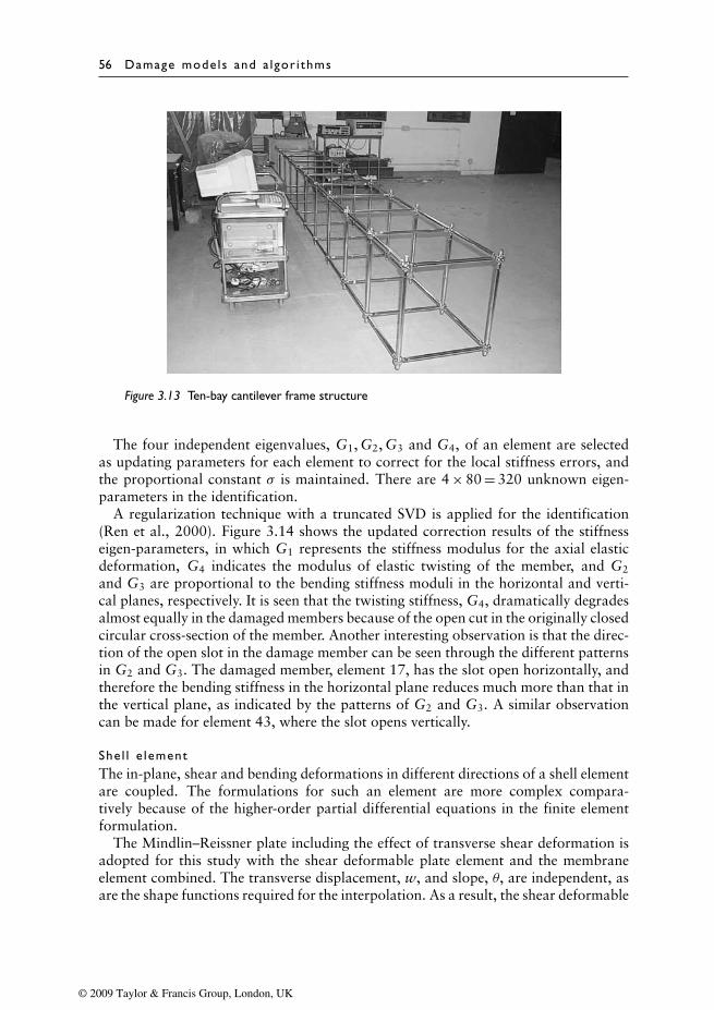
56 Damage mode ls and a lgor i thms
Figure 3.13 Ten-bay cantilever frame structure
The four independent eigenvalues, G1, G2, G3 and G4, of an element are selectedas updating parameters for each element to correct for the local stiffness errors, andthe proportional constant σ is maintained. There are 4 × 80 = 320 unknown eigen-parameters in the identification.
A regularization technique with a truncated SVD is applied for the identification(Ren et al., 2000). Figure 3.14 shows the updated correction results of the stiffnesseigen-parameters, in which G1 represents the stiffness modulus for the axial elasticdeformation, G4 indicates the modulus of elastic twisting of the member, and G2
and G3 are proportional to the bending stiffness moduli in the horizontal and verti-cal planes, respectively. It is seen that the twisting stiffness, G4, dramatically degradesalmost equally in the damaged members because of the open cut in the originally closedcircular cross-section of the member. Another interesting observation is that the direc-tion of the open slot in the damage member can be seen through the different patternsin G2 and G3. The damaged member, element 17, has the slot open horizontally, andtherefore the bending stiffness in the horizontal plane reduces much more than that inthe vertical plane, as indicated by the patterns of G2 and G3. A similar observationcan be made for element 43, where the slot opens vertically.
She l l e lementThe in-plane, shear and bending deformations in different directions of a shell elementare coupled. The formulations for such an element are more complex compara-tively because of the higher-order partial differential equations in the finite elementformulation.
The Mindlin–Reissner plate including the effect of transverse shear deformation isadopted for this study with the shear deformable plate element and the membraneelement combined. The transverse displacement, w, and slope, θ, are independent, asare the shape functions required for the interpolation. As a result, the shear deformable
© 2009 Taylor & Francis Group, London, UK
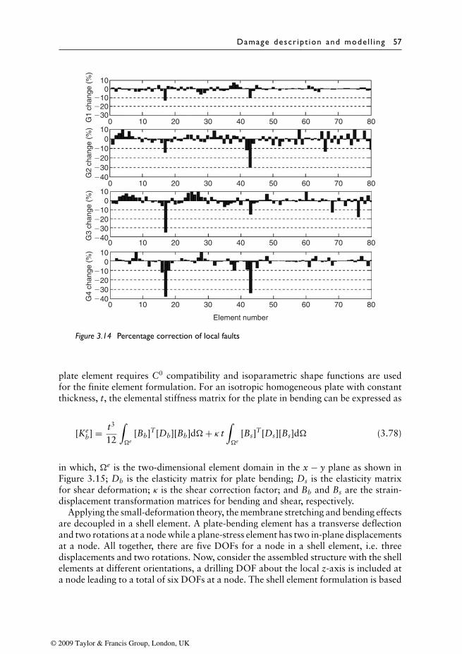
Damage descr ipt ion and mode l l ing 57
100
�10�20�30
0 10 20 30 40 50 60 70 80
0 10 20 30 40 50 60 70 80
0 10 20 30 40 50 60 70 80
0 10 20 30 40 50 60 70 80
G1
chan
ge (
%)
100
�10�20
�40�30
G2
chan
ge (
%)
100
�10�20
�40�30
G3
chan
ge (
%)
100
�10�20
�40�30
G4
chan
ge (
%)
Element number
Figure 3.14 Percentage correction of local faults
plate element requires C0 compatibility and isoparametric shape functions are usedfor the finite element formulation. For an isotropic homogeneous plate with constantthickness, t, the elemental stiffness matrix for the plate in bending can be expressed as
[Keb] = t3
12
∫�e
[Bb]T [Db][Bb]d�+ κ t∫�e
[Bs]T [Ds][Bs]d� (3.78)
in which, �e is the two-dimensional element domain in the x − y plane as shown inFigure 3.15; Db is the elasticity matrix for plate bending; Ds is the elasticity matrixfor shear deformation; κ is the shear correction factor; and Bb and Bs are the strain-displacement transformation matrices for bending and shear, respectively.
Applying the small-deformation theory, the membrane stretching and bending effectsare decoupled in a shell element. A plate-bending element has a transverse deflectionand two rotations at a node while a plane-stress element has two in-plane displacementsat a node. All together, there are five DOFs for a node in a shell element, i.e. threedisplacements and two rotations. Now, consider the assembled structure with the shellelements at different orientations, a drilling DOF about the local z-axis is included ata node leading to a total of six DOFs at a node. The shell element formulation is based
© 2009 Taylor & Francis Group, London, UK
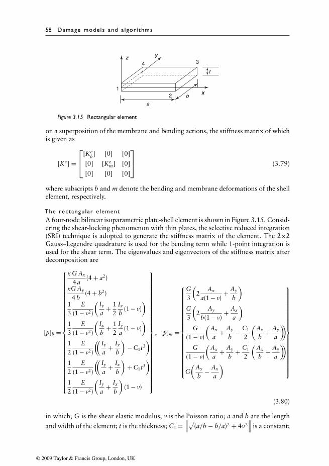
58 Damage mode ls and a lgor i thms
x
yz34
21
t
b
a
Figure 3.15 Rectangular element
on a superposition of the membrane and bending actions, the stiffness matrix of whichis given as
[Ke] =[Ke
b] [0] [0]
[0] [Kem] [0]
[0] [0] [0]
(3.79)
where subscripts b and m denote the bending and membrane deformations of the shellelement, respectively.
The rectangu lar e lementA four-node bilinear isoparametric plate-shell element is shown in Figure 3.15. Consid-ering the shear-locking phenomenon with thin plates, the selective reduced integration(SRI) technique is adopted to generate the stiffness matrix of the element. The 2×2Gauss–Legendre quadrature is used for the bending term while 1-point integration isused for the shear term. The eigenvalues and eigenvectors of the stiffness matrix afterdecomposition are
[p]b =
κG Ax
4 a(4 + a2)
κG Ay
4 b(4 + b2)
13
E(1 − ν2)
(Iy
a+ 1
2Ix
b(1 − ν)
)13
E(1 − ν2)
(Ix
b+ 1
2Iy
a(1 − ν)
)12
E(1 − ν2)
((Iy
a+ Ix
b
)− C1t3
)12
E(1 − ν2)
((Iy
a+ Ix
b
)+ C1t3
)12
E(1 − ν2)
(Iy
a+ Ix
b
)(1 − ν)
, [p]m =
G3
(2
Ax
a(1 − ν) + Ay
b
)G3
(2
Ay
b(1 − ν) + Ax
a
)G
(1 − ν)(
Ax
a+ Ay
b− C1
2
(Ax
b+ Ay
a
))G
(1 − ν)(
Ax
a+ Ay
b+ C1
2
(Ax
b+ Ay
a
))G(
Ay
b− Ax
a
)
(3.80)
in which, G is the shear elastic modulus; ν is the Poisson ratio; a and b are the length
and width of the element; t is the thickness; C1 =∥∥∥√(a/b − b/a)2 + 4ν2
∥∥∥ is a constant;
© 2009 Taylor & Francis Group, London, UK
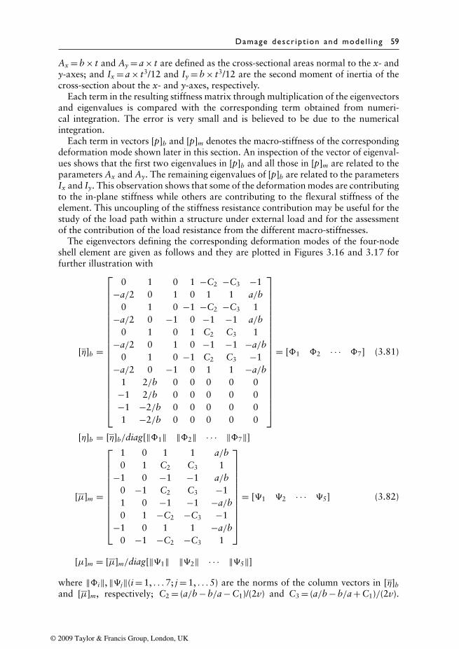
Damage descr ipt ion and mode l l ing 59
Ax = b × t and Ay = a × t are defined as the cross-sectional areas normal to the x- andy-axes; and Ix = a × t3/12 and Iy = b × t3/12 are the second moment of inertia of thecross-section about the x- and y-axes, respectively.
Each term in the resulting stiffness matrix through multiplication of the eigenvectorsand eigenvalues is compared with the corresponding term obtained from numeri-cal integration. The error is very small and is believed to be due to the numericalintegration.
Each term in vectors [p]b and [p]m denotes the macro-stiffness of the correspondingdeformation mode shown later in this section. An inspection of the vector of eigenval-ues shows that the first two eigenvalues in [p]b and all those in [p]m are related to theparameters Ax and Ay. The remaining eigenvalues of [p]b are related to the parametersIx and Iy. This observation shows that some of the deformation modes are contributingto the in-plane stiffness while others are contributing to the flexural stiffness of theelement. This uncoupling of the stiffness resistance contribution may be useful for thestudy of the load path within a structure under external load and for the assessmentof the contribution of the load resistance from the different macro-stiffnesses.
The eigenvectors defining the corresponding deformation modes of the four-nodeshell element are given as follows and they are plotted in Figures 3.16 and 3.17 forfurther illustration with
[η]b =
0 1 0 1 −C2 −C3 −1−a/2 0 1 0 1 1 a/b
0 1 0 −1 −C2 −C3 1−a/2 0 −1 0 −1 −1 a/b
0 1 0 1 C2 C3 1−a/2 0 1 0 −1 −1 −a/b
0 1 0 −1 C2 C3 −1−a/2 0 −1 0 1 1 −a/b
1 2/b 0 0 0 0 0−1 2/b 0 0 0 0 0−1 −2/b 0 0 0 0 01 −2/b 0 0 0 0 0
= [�1 �2 · · · �7] (3.81)
[η]b = [η]b/diag[‖�1‖ ‖�2‖ · · · ‖�7‖]
[µ]m =
1 0 1 1 a/b0 1 C2 C3 1
−1 0 −1 −1 a/b0 −1 C2 C3 −11 0 −1 −1 −a/b0 1 −C2 −C3 −1
−1 0 1 1 −a/b0 −1 −C2 −C3 1
= [�1 �2 · · · �5] (3.82)
[µ]m = [µ]m/diag[‖�1‖ ‖�2‖ · · · ‖�5‖]
where ‖�i‖, ‖�j‖(i = 1, . . .7; j = 1, . . .5) are the norms of the column vectors in [η]b
and [µ]m, respectively; C2 = (a/b − b/a − C1)/(2v) and C3 = (a/b − b/a + C1)/(2v).
© 2009 Taylor & Francis Group, London, UK
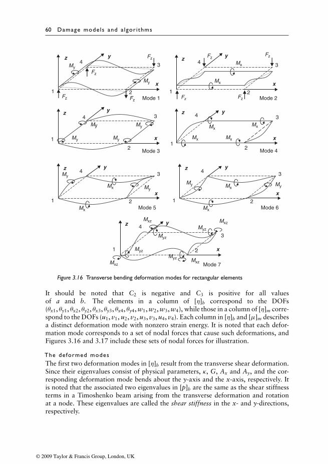
60 Damage mode ls and a lgor i thms
z y
x
Mode 1
4 3
2 1
Mode 4
x
y z 4 3
2 1
Mode 3
x
y z 4 3
2
1
Mode 7
x
y z 4
3
2 1
Mode 2
x
y z 4 3
2 1
Mode 6
x
y z 4 3
2 1 Mode 5
x
y z 4 3
2 1
My
My
My Mx
MxMx
MxMx
MyMy
My
My My
My
MyMxMx
Mx Mx
MxzMxz
MxzMxz
Myz
Myz
Myz
Myz
Mx
Fz Fz
FzFzFzFz
Fz
Fz
Figure 3.16 Transverse bending deformation modes for rectangular elements
It should be noted that C2 is negative and C3 is positive for all valuesof a and b. The elements in a column of [η]b correspond to the DOFs(θx1, θy1, θx2, θy2, θx3, θy3, θx4, θy4, w1, w2, w3, w4), while those in a column of [η]m corre-spond to the DOFs (u1, v1, u2, v2, u3, v3, u4, v4). Each column in [η]b and [µ]m describesa distinct deformation mode with nonzero strain energy. It is noted that each defor-mation mode corresponds to a set of nodal forces that cause such deformations, andFigures 3.16 and 3.17 include these sets of nodal forces for illustration.
The deformed modesThe first two deformation modes in [η]b result from the transverse shear deformation.Since their eigenvalues consist of physical parameters, κ, G, Ax and Ay, and the cor-responding deformation mode bends about the y-axis and the x-axis, respectively. Itis noted that the associated two eigenvalues in [p]b are the same as the shear stiffnessterms in a Timoshenko beam arising from the transverse deformation and rotationat a node. These eigenvalues are called the shear stiffness in the x- and y-directions,respectively.
© 2009 Taylor & Francis Group, London, UK
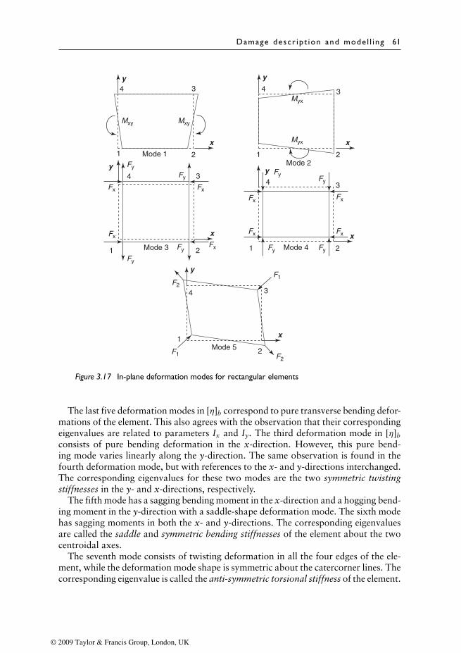
Damage descr ipt ion and mode l l ing 61
Mode 1
MxyMxy
Mode 4
Mode 2
Mode 5
F1F2
F2F1
Myx
Myx
Mode 3
1 2
4
x
y3
2
4
1
x
y
3
2
4
1 x
y
3
2
4
1
x
y
3
2
4
1
x
y3
Fy
Fy
Fy
FyFy
Fy
FyFy
Fx Fx
Fx Fx
FxFx
Fx
Fx
Figure 3.17 In-plane deformation modes for rectangular elements
The last five deformation modes in [η]b correspond to pure transverse bending defor-mations of the element. This also agrees with the observation that their correspondingeigenvalues are related to parameters Ix and Iy. The third deformation mode in [η]b
consists of pure bending deformation in the x-direction. However, this pure bend-ing mode varies linearly along the y-direction. The same observation is found in thefourth deformation mode, but with references to the x- and y-directions interchanged.The corresponding eigenvalues for these two modes are the two symmetric twistingstiffnesses in the y- and x-directions, respectively.
The fifth mode has a sagging bending moment in the x-direction and a hogging bend-ing moment in the y-direction with a saddle-shape deformation mode. The sixth modehas sagging moments in both the x- and y-directions. The corresponding eigenvaluesare called the saddle and symmetric bending stiffnesses of the element about the twocentroidal axes.
The seventh mode consists of twisting deformation in all the four edges of the ele-ment, while the deformation mode shape is symmetric about the catercorner lines. Thecorresponding eigenvalue is called the anti-symmetric torsional stiffness of the element.
© 2009 Taylor & Francis Group, London, UK
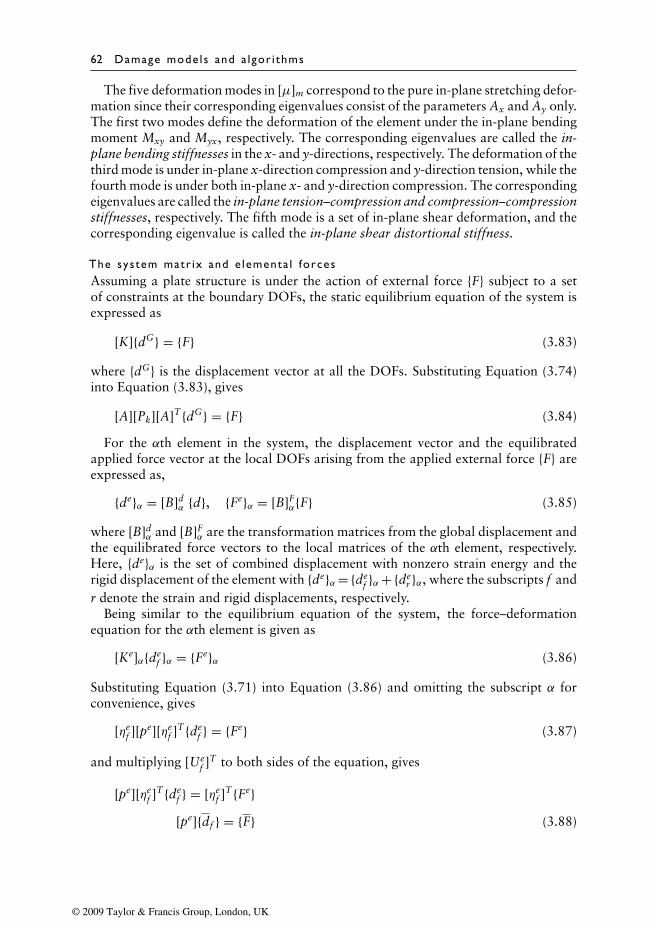
62 Damage mode ls and a lgor i thms
The five deformation modes in [µ]m correspond to the pure in-plane stretching defor-mation since their corresponding eigenvalues consist of the parameters Ax and Ay only.The first two modes define the deformation of the element under the in-plane bendingmoment Mxy and Myx, respectively. The corresponding eigenvalues are called the in-plane bending stiffnesses in the x- and y-directions, respectively. The deformation of thethird mode is under in-plane x-direction compression and y-direction tension, while thefourth mode is under both in-plane x- and y-direction compression. The correspondingeigenvalues are called the in-plane tension–compression and compression–compressionstiffnesses, respectively. The fifth mode is a set of in-plane shear deformation, and thecorresponding eigenvalue is called the in-plane shear distortional stiffness.
The system matr ix and e lementa l forcesAssuming a plate structure is under the action of external force {F} subject to a setof constraints at the boundary DOFs, the static equilibrium equation of the system isexpressed as
[K]{dG} = {F} (3.83)
where {dG} is the displacement vector at all the DOFs. Substituting Equation (3.74)into Equation (3.83), gives
[A][Pk][A]T{dG} = {F} (3.84)
For the αth element in the system, the displacement vector and the equilibratedapplied force vector at the local DOFs arising from the applied external force {F} areexpressed as,
{de}α = [B]dα {d}, {Fe}α = [B]F
α{F} (3.85)
where [B]dα and [B]F
α are the transformation matrices from the global displacement andthe equilibrated force vectors to the local matrices of the αth element, respectively.Here, {de}α is the set of combined displacement with nonzero strain energy and therigid displacement of the element with {de}α= {de
f }α+ {der }α, where the subscripts f and
r denote the strain and rigid displacements, respectively.Being similar to the equilibrium equation of the system, the force–deformation
equation for the αth element is given as
[Ke]α{def }α = {Fe}α (3.86)
Substituting Equation (3.71) into Equation (3.86) and omitting the subscript α forconvenience, gives
[ηef ][p
e][ηef ]
T{def } = {Fe} (3.87)
and multiplying [Uef ]T to both sides of the equation, gives
[pe][ηef ]
T{def } = [ηe
f ]T{Fe}
[pe]{df } = {F} (3.88)
© 2009 Taylor & Francis Group, London, UK
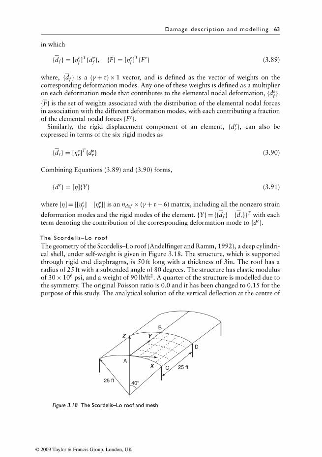
Damage descr ipt ion and mode l l ing 63
in which
{df } = [ηef ]
T{def }, {F} = [ηe
f ]T{Fe} (3.89)
where, {df } is a (γ + τ) × 1 vector, and is defined as the vector of weights on thecorresponding deformation modes. Any one of these weights is defined as a multiplieron each deformation mode that contributes to the elemental nodal deformation, {de
f }.{F} is the set of weights associated with the distribution of the elemental nodal forcesin association with the different deformation modes, with each contributing a fractionof the elemental nodal forces {Fe}.
Similarly, the rigid displacement component of an element, {der }, can also be
expressed in terms of the six rigid modes as
{dr} = [ηer]
T{der } (3.90)
Combining Equations (3.89) and (3.90) forms,
{de} = [η]{Y} (3.91)
where [η] = [[ηef ] [ηe
r]] is an ndof × (γ + τ+ 6) matrix, including all the nonzero strain
deformation modes and the rigid modes of the element. {Y} = {{df } {dr}}T with eachterm denoting the contribution of the corresponding deformation mode to {de}.
The Scorde l i s–Lo roofThe geometry of the Scordelis–Lo roof (Andelfinger and Ramm, 1992), a deep cylindri-cal shell, under self-weight is given in Figure 3.18. The structure, which is supportedthrough rigid end diaphragms, is 50 ft long with a thickness of 3in. The roof has aradius of 25 ft with a subtended angle of 80 degrees. The structure has elastic modulusof 30 × 106 psi, and a weight of 90 lb/ft2. A quarter of the structure is modelled due tothe symmetry. The original Poisson ratio is 0.0 and it has been changed to 0.15 for thepurpose of this study. The analytical solution of the vertical deflection at the centre of
X
Y
25 ft
Z
40�
25 ft
B
D
C A
Figure 3.18 The Scordelis–Lo roof and mesh
© 2009 Taylor & Francis Group, London, UK
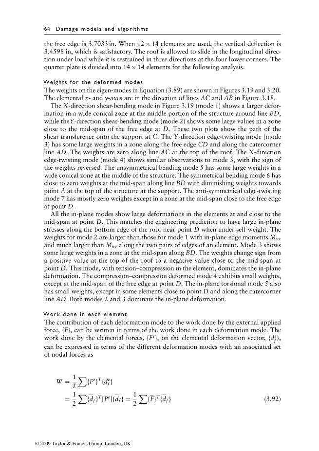
64 Damage mode ls and a lgor i thms
the free edge is 3.7033 in. When 12 × 14 elements are used, the vertical deflection is3.4598 in, which is satisfactory. The roof is allowed to slide in the longitudinal direc-tion under load while it is restrained in three directions at the four lower corners. Thequarter plate is divided into 14 × 14 elements for the following analysis.
Weights for the de formed modesThe weights on the eigen-modes in Equation (3.89) are shown in Figures 3.19 and 3.20.The elemental x- and y-axes are in the direction of lines AC and AB in Figure 3.18.
The X-direction shear-bending mode in Figure 3.19 (mode 1) shows a larger defor-mation in a wide conical zone at the middle portion of the structure around line BD,while theY-direction shear-bending mode (mode 2) shows some large values in a zoneclose to the mid-span of the free edge at D. These two plots show the path of theshear transference onto the support at C. The Y-direction edge-twisting mode (mode3) has some large weights in a zone along the free edge CD and along the catercornerline AD. The weights are zero along line AC at the top of the roof. The X-directionedge-twisting mode (mode 4) shows similar observations to mode 3, with the sign ofthe weights reversed. The unsymmetrical bending mode 5 has some large weights in awide conical zone at the middle of the structure. The symmetrical bending mode 6 hasclose to zero weights at the mid-span along line BD with diminishing weights towardspoint A at the top of the structure at the support. The anti-symmetrical edge-twistingmode 7 has mostly zero weights except in a zone at the mid-span close to the free edgeat point D.
All the in-plane modes show large deformations in the elements at and close to themid-span at point D. This matches the engineering prediction to have large in-planestresses along the bottom edge of the roof near point D when under self-weight. Theweights for mode 2 are larger than those for mode 1 with in-plane edge moments Myx
and much larger than Mxy along the two pairs of edges of an element. Mode 3 showssome large weights in a zone at the mid-span along BD. The weights change sign froma positive value at the top of the roof to a negative value close to the mid-span atpoint D. This mode, with tension–compression in the element, dominates the in-planedeformation. The compression–compression deformed mode 4 exhibits small weights,except at the mid-span of the free edge at point D. The in-plane torsional mode 5 alsohas small weights, except in some elements close to point D and along the catercornerline AD. Both modes 2 and 3 dominate the in-plane deformation.
Work done in each e lementThe contribution of each deformation mode to the work done by the external appliedforce, {F}, can be written in terms of the work done in each deformation mode. Thework done by the elemental forces, {Fe}, on the elemental deformation vector, {de
f },can be expressed in terms of the different deformation modes with an associated setof nodal forces as
W = 12
∑{Fe}T{de
f }
= 12
∑{df }T [Pe]{df } = 1
2
∑{F}T{df } (3.92)
© 2009 Taylor & Francis Group, London, UK
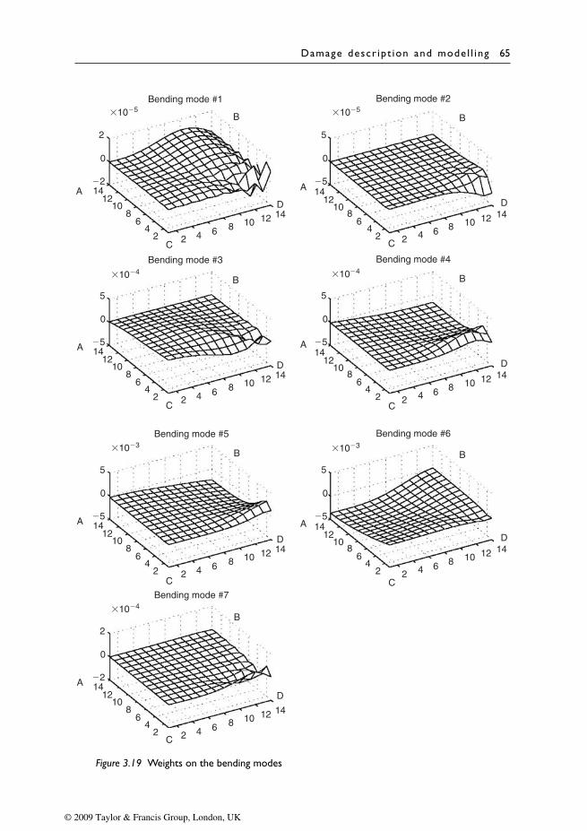
Damage descr ipt ion and mode l l ing 65
Bending mode #1
2
0
�2
�10�5
A
C2 4 6 8 10 12 14
1412
108
64
2
D
B
Bending mode #2
5
0
�5
�10�5
A
C 2 4 6 8 10 12 14
1412
108
64
2
D
B
Bending mode #3
5
0
�5
�10�4
A
C2 4 6 8 10 12 14
1412
108
64
2
D
B
Bending mode #4
5
0
�5
�10�4
A
C2 4 6 8 10 12 14
1412
108
64
2
D
B
Bending mode #5
5
0
�5
�10�3
A
C2 4 6 8 10 12 14
1412
108
64
2
D
B
Bending mode #7
2
0
�2
�10�4
A
C 2 4 6 8 10 12 14
1412
108
64
2
D
B
Bending mode #6
5
0
�5
�10�3
A
C2 4 6 8 10 12 14
1412
108
64
2
D
B
Figure 3.19 Weights on the bending modes
© 2009 Taylor & Francis Group, London, UK
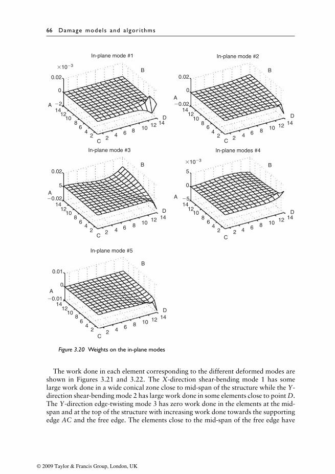
66 Damage mode ls and a lgor i thms
In-plane mode #1
0
�2
�10�3
�10�3
A
C2 4 6 8 10 12 14
1412
108
64
2
D
B
In-plane mode #2
0.02
�0.02
0A
C 2 4 6 8 10 12 14
1412
108
64
2
D
B
In-plane mode #3
0.02
0.02
5
�0.02A
C2 4 6 8 10 12 14
1412
108
64
2
D
B
In-plane mode #5
0.01
0
�0.01A
C2 4 6 8 10 12 14
1412
108
64
2
D
B
In-plane modes #4
5
0
�5A
C2 4 6 8 10 12 14
1412
108
64
2
D
B
Figure 3.20 Weights on the in-plane modes
The work done in each element corresponding to the different deformed modes areshown in Figures 3.21 and 3.22. The X-direction shear-bending mode 1 has somelarge work done in a wide conical zone close to mid-span of the structure while the Y-direction shear-bending mode 2 has large work done in some elements close to point D.The Y-direction edge-twisting mode 3 has zero work done in the elements at the mid-span and at the top of the structure with increasing work done towards the supportingedge AC and the free edge. The elements close to the mid-span of the free edge have
© 2009 Taylor & Francis Group, London, UK
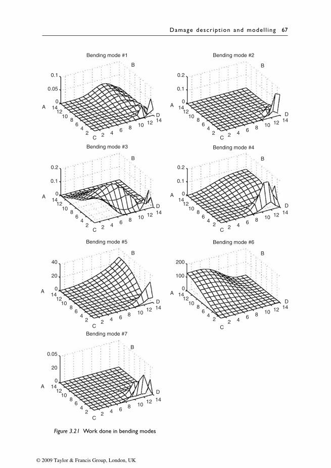
Damage descr ipt ion and mode l l ing 67
Bending mode #1
0.1
0.05
0A
C 2 4 6 8 10 12 14
1412
108
64
2
D
B
Bending mode #2
0.2
0.1
0A
C 2 4 6 8 10 12 14
1412
108
64
2
D
B
Bending mode #3
0.2
0.1
0A
C 2 4 6 8 10 12 14
1412
108
64
2
D
B
Bending mode #4
0.2
0.1
0A
C 2 4 6 8 10 12 14
1412
108
64
2
D
B
Bending mode #5
40
20
0A
C2 4 6 8 10 12 14
1412
108
64
2
D
B
Bending mode #7
0.05
20
0A
C2 4 6 8 10 12 14
1412
108
64
2
D
B
Bending mode #6
200
100
0A
C2 4 6 8 10 12 14
1412
108
64
2
D
B
Figure 3.21 Work done in bending modes
© 2009 Taylor & Francis Group, London, UK
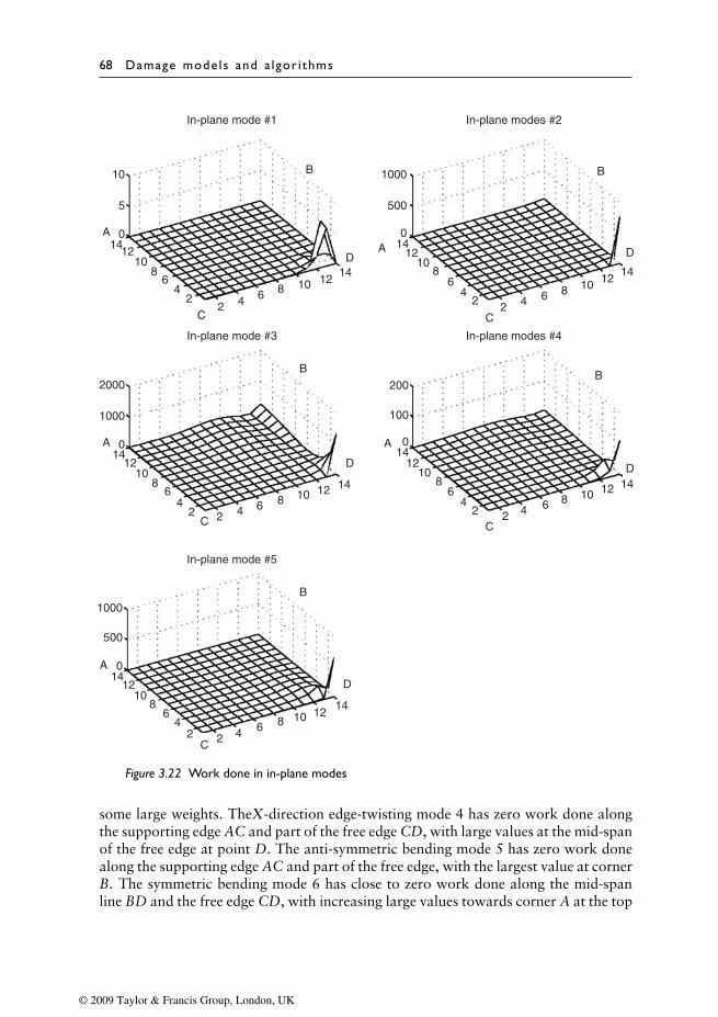
68 Damage mode ls and a lgor i thms
In-plane mode #1
10
5
0A
C2 4 6 8 10 12
14
1412
108
64
2
D
B
In-plane modes #2
1000
500
0A
C2 4 6 8 10 12
14
1412
108
64
2
D
B
In-plane mode #3
2000
1000
0A
C 2 4 6 8 10 12 14
1412
108
64
2
D
B
In-plane mode #5
1000
500
0A
C 2 4 6 8 10 1214
1412
108
64
2
D
B
In-plane modes #4
200
100
0A
C2 4 6 8 10 12 14
1412
108
64
2
D
B
Figure 3.22 Work done in in-plane modes
some large weights. TheX-direction edge-twisting mode 4 has zero work done alongthe supporting edge AC and part of the free edge CD, with large values at the mid-spanof the free edge at point D. The anti-symmetric bending mode 5 has zero work donealong the supporting edge AC and part of the free edge, with the largest value at cornerB. The symmetric bending mode 6 has close to zero work done along the mid-spanline BD and the free edge CD, with increasing large values towards corner A at the top
© 2009 Taylor & Francis Group, London, UK
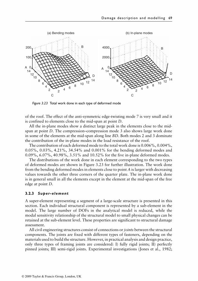
Damage descr ipt ion and mode l l ing 69
(a) Bending modes
200
100
0A
C2
4 68 10 12
14
1412
108
64
2
D
B
(b) In-plane modes
4000
2000
0A
C
24 6
810 12
14
1412
108
64
2
D
B
Figure 3.23 Total work done in each type of deformed mode
of the roof. The effect of the anti-symmetric edge-twisting mode 7 is very small and itis confined to elements close to the mid-span at point D.
All the in-plane modes show a distinct large peak in the elements close to the mid-span at point D. The compression–compression mode 3 also shows large work donein some of the elements at the mid-span along line BD. Both modes 2 and 3 dominatethe contribution of the in-plane modes in the load resistance of the roof.
The contribution of each deformed mode to the total work done is 0.006%, 0.004%,0.05%, 0.03%, 4.21%, 34.54% and 0.001% for the bending deformed modes and0.09%, 6.07%, 40.98%, 3.51% and 10.52% for the five in-plane deformed modes.
The distributions of the work done in each element corresponding to the two typesof deformed modes are shown in Figure 3.23 for further illustration. The work donefrom the bending deformed modes in elements close to point A is larger with decreasingvalues towards the other three corners of the quarter plate. The in-plane work doneis in general small in all the elements except in the element at the mid-span of the freeedge at point D.
3.2.3 Super-element
A super-element representing a segment of a large-scale structure is presented in thissection. Each individual structural component is represented by a sub-element in themodel. The large number of DOFs in the analytical model is reduced, while themodal sensitivity relationship of the structural model to small physical changes can beretained at the sub-element level. These properties are significant to structural damageassessment.
All civil engineering structures consist of connections or joints between the structuralcomponents. The joints are fixed with different types of fasteners, depending on thematerials used to build the structure. However, in practical analysis and design practice,only three types of framing joints are considered: I) fully rigid joints; II) perfectlypinned joints; III) semi-rigid joints. Experimental investigations (Jones et al., 1982;
© 2009 Taylor & Francis Group, London, UK
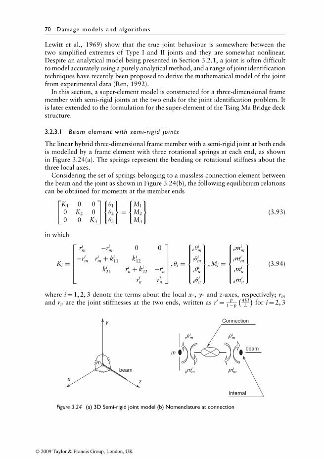
70 Damage mode ls and a lgor i thms
Lewitt et al., 1969) show that the true joint behaviour is somewhere between thetwo simplified extremes of Type I and II joints and they are somewhat nonlinear.Despite an analytical model being presented in Section 3.2.1, a joint is often difficultto model accurately using a purely analytical method, and a range of joint identificationtechniques have recently been proposed to derive the mathematical model of the jointfrom experimental data (Ren, 1992).
In this section, a super-element model is constructed for a three-dimensional framemember with semi-rigid joints at the two ends for the joint identification problem. Itis later extended to the formulation for the super-element of the Tsing Ma Bridge deckstructure.
3.2.3.1 Beam element wi th semi - r ig id jo in ts
The linear hybrid three-dimensional frame member with a semi-rigid joint at both endsis modelled by a frame element with three rotational springs at each end, as shownin Figure 3.24(a). The springs represent the bending or rotational stiffness about thethree local axes.
Considering the set of springs belonging to a massless connection element betweenthe beam and the joint as shown in Figure 3.24(b), the following equilibrium relationscan be obtained for moments at the member endsK1 0 0
0 K2 00 0 K3
θ1θ2θ3
=
M1
M2
M3
(3.93)
in which
Ki =
rim −ri
m 0 0
−rim ri
m + ki11 ki
12
ki21 ri
n + ki22 −ri
n
−rin ri
n
, θi =
eθ
im
iθim
iθin
eθin
, Mi =
emi
m
imim
imin
emin
(3.94)
where i = 1, 2, 3 denote the terms about the local x-, y- and z-axes, respectively; rm
and rn are the joint stiffnesses at the two ends, written as ri = p1 − p
( 4EIL
)for i = 2, 3
mbeam
Connection
Internal
z
y
x
beamm
emim
euim
imim
iuim
Figure 3.24 (a) 3D Semi-rigid joint model (b) Nomenclature at connection
© 2009 Taylor & Francis Group, London, UK
Damage descr ipt ion and mode l l ing 71
and r1 = p1 − p
(GJL
), in which p is the fixity factor, which is zero for perfectly pinned
joints and one for perfectly rigid joints; the second moment of inertia of the membercross-section about the x- and y-axes are assumed to be the same; eθ
im, eθ
in, iθ
im and
iθin are the external and internal rotation about the ith axis, respectively, as shown in
Figure 3.24(b); and kipq are the corresponding components of the stiffness matrix of a
conventional beam element if the bowing effect is ignored, given by
k1pq = GJ
L
[1 −1
−1 1
], ki
pq = EIL
[4 22 4
], (i = 2, 3) (3.95)
Since the external forces and moments are applied at the external nodes of the jointedmember only, the applied moments about each axis at the internal nodes connectingthe beam element and the spring can be obtained by considering equilibrium of theconnection shown in Figure 3.24(b):[
rim + ki
11 ki12
ki21 ri
n + ki22
]{iθ
im
iθin
}−[
rim 0
0 rin
]{eθ
im
eθin
}={
0
0
}, (i = 1, 2, 3) (3.96)
or {iθ
im
iθin
}=[
rim + ki
11 ki12
ki21 ri
n + ki22
]−1 [rim 0
0 rin
]{eθ
im
eθin
}, (i = 1, 2, 3) (3.97)
Substituting Equation (3.97) into Equation (3.93), the stiffness terms related to theinternal nodes are eliminated, and the condensed stiffness matrix relating the momentsand rotations about the external nodes can be written as:
em1m
em2m
em3m
em1n
em2n
em3n
=[Kmn K21
K12 Knm
]
eθ1m
eθ2m
eθ3m
eθ1n
eθ2n
eθ3n
(3.98)
where Kij =r1
i − (r1i )2(r1
j + k122)/ρ1 0 0
0 r2i − (r2
i )2(r2j + k2
22)/ρ2 0
0 0 r3i − (r3
i )2(r3j + k3
22)/ρ3
for
i = m, nj = m, n
i = j
,
and K12 = K21 =k1
12r1mr1
n/ρ1 0 0
0 k212r2
mr2n/ρ2 0
0 0 k312r3
mr3n/ρ3
,
© 2009 Taylor & Francis Group, London, UK
72 Damage mode ls and a lgor i thms
where
ρi = det
[ki
11 + rim ki
12
ki21 ki
22 + rin
](3.99)
Adding the terms for the axial force to Equation (3.98), and transforming the result-ing 8×8 matrix to the nodal DOFs of the element, the stiffness matrix of the semi-rigidjointed beam element can be written as:
Ke = T ·
EA/L 0 0 0
0 Kmn 0 K21
0 0 EA/L 00 K12 0 Knm
8×8
· TT (3.100)
in which T is the 12×8 transformation matrix mapping the six external moments andtwo axial forces to the nodal forces and moments in the local coordinates, respectively,given by
T =
1 0 0 0 0 0 0 0 0 0 0 00 0 0 1 0 0 0 0 0 0 0 00 1/L 0 0 1 0 0 −1/L 0 0 0 00 0 1/L 0 0 1 0 0 −1/L 0 0 00 0 0 0 0 0 1 0 0 0 0 00 0 0 0 0 0 0 0 0 1 0 00 1/L 0 0 0 0 0 −1/L 0 0 1 00 0 1/L 0 0 0 0 0 −1/L 0 0 1
(3.101)
It can be easily verified that the semi-rigid jointed beam element expressed in Equation(3.100) is equal to a pinned joint beam element if the spring stiffness is zero and to arigid joint beam element if the spring stiffness is infinite.
Model l ing o f a ten-bay cant i lever f rame structureThe ten-bay cantilever frame structure shown in Figure 3.13 is divided into five super-elements in the longitudinal direction, each consists of four longitudinal-beam typesub-elements and twelve cross-beam type sub-elements connected by semi-rigid joints.The super-element model of the beam segment is shown in Figure 3.25. There are fourmaster nodes at the corners and one slave node at the centre of the end-section. Eachmaster node has three translational DOFs parallel to the local coordinate axes. Eachslave node has three rotational DOFs about the three global axes of the end-section.There are 15 DOFs in each end-section, and there are 10 nodes (8 master and 2 slave)and 30 DOFs for each super-element. Altogether, there are 30 nodes and 75 DOFs forthe whole structure. This model is much smaller than the conventional finite elementmodel which has 240 DOFs.
The super-element model has been used to achieve good updated results for the lowerfrequency modes but not for the higher frequency modes (Law et al., 2001c). A perfectlyrefined model that represents the real structure is not achieved, and the updated resultshave errors which increase as the modal order increases. The first type of error is due tothe incorrect assumptions made while condensing the finite element DOFs to those of
© 2009 Taylor & Francis Group, London, UK

Damage descr ipt ion and mode l l ing 73
Main cross-beam
Intermediate cross-beam
Longitudinal beam
(a)
1
2 3
4
5
7
6
8
910
(b)
fY
fX
2 3
45
1
Y
ϕ
Figure 3.25 Super-element model of truss segment
the super-element. The second type of error is from the difference in the macro updatingparameter in different members resulting from different ways of assembling the teststructure. But the more significant error comes from the incomplete measurement,particularly from the rotational DOFs which cannot be measured in this study.
Half of the DOFs in a conventional finite element model of the truss are rotationalDOFs. The super-element model has the advantage that the rotational DOFs are con-densed and it has a smaller proportion of rotational DOFs than the conventional finiteelement model. There are only 15 rotational DOFs within a total of 75 DOFs for thewhole test structure. It is therefore considered that the use of all the lower mode shapesin the identification reduces the first type of error, while the other types of errors cannotbe avoided.
3.2.3.2 The Ts ing Ma br idge deck
The formulation of the bridge deck model (Lantau, 1998) of the Tsing Ma suspensionbridge in Hong Kong is presented for further illustration of the super-element mod-elling. The bridge serves as the link between the new airport of Hong Kong and thecommercial centres. The bridge deck is a two-level enclosed structure, which carriesa dual three-lane highway at the upper level and two railway tracks and two trafficlanes at the lower level. The whole deck structure can be divided into segments betweenadjacent sets of suspenders 18m apart, the arrangement of which is shown in Figure3.26(a). Each segment consists of 66 structural components of longitudinal beams,cross-beams, bracings and stiffened plates.
All the nodes of the super-element are allocated on the two outermost sections alongthe longitudinal axis. Each end section consists of a number of nodes and several sub-elements as shown in Figure 3.26(b), depending on the specific deck configuration. Inthe type of bridge deck under consideration, there are ten master nodes and one slavenode in the section. The primary longitudinal beams and auxiliary longitudinal beamsare connected to nodes 2, 5, 7 and 10 and 3, 4, 8 and 9, respectively. Nodes 6 and 11are at the intersection of cross-beams at the edges, and there are 14 cross-beams in thesection, which are represented by line segments in the figure (the thicker lines indicatethat there is also a stiffened plate between two adjacent longitudinal beams). Bracingmembers and stiffened plates are not shown in this figure, as they are not in the same
© 2009 Taylor & Francis Group, London, UK
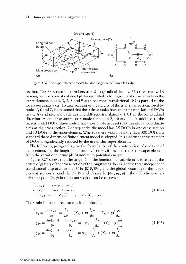
74 Damage mode ls and a lgor i thms
(a) (b)
fY
fX
11
2 3 4 5
6
78910
1
Main cross-beamIntermediatecross-beam
Longitudinalbeam
Bracing type(1)
Bracing type(2)
ϕ
Figure 3.26 The super-element model for deck segment of Tsing Ma Bridge
section. The 66 structural members are: 8 longitudinal beams, 38 cross-beams, 16bracing members and 4 stiffened plates modelled as four groups of sub-elements in thesuper-element. Nodes 3, 4, 8 and 9 each has three translational DOFs parallel to thelocal coordinate axes. To take account of the rigidity of the triangular part enclosed bynodes 5, 6 and 7, it is assumed that these three nodes have the same translational DOFsin the X-Y plane, and each has one different translational DOF in the longitudinaldirection. A similar assumption is made for nodes 2, 10 and 11. In addition to themaster nodal DOFs, slave node 1 has three DOFs around the three global coordinateaxes of the cross-section. Consequently, the model has 25 DOFs in one cross-sectionand 50 DOFs in the super-element. Whereas there would be more than 300 DOFs if astandard three-dimension finite element model is adopted. It is evident that the numberof DOFs is significantly reduced by the use of this super-element.
The following paragraphs give the formulation of the contribution of one type ofsub-element, i.e. the longitudinal beams, to the stiffness matrix of the super-elementfrom the variational principle of minimum potential energy.
Figure 3.27 shows that the origin C of the longitudinal sub-element is seated at thecentre of gravity of the cross-section of the longitudinal beam. Let the three independenttranslational displacements of C be {u, v, w}T , and the global rotations of the super-element section around the X-,Y- and Z-axes be {φX,φY ,ϕ}T , the deflections of anarbitrary point (x, y) in the beam section can be expressed as
u(x, y) = u − ϕ(YC + y)v(x, y) = v + ϕ(XC + x)w(x, y) = w + φX(YC + y) − φY (XC + x)
(3.102)
The strain in the z-direction can be obtained as
εz = ∂w(x, y)∂z
= dwdz
− (XC + x)dφY
dz+ (YC + y)
dφX
dz
γzx = ∂w(x, y)∂x
+ ∂u(x, y)∂z
= −φY + dudz
− (YC + y)dϕdz
γzy = ∂w(x, y)∂y
+ ∂v(x, y)∂z
= φX + dvdz
+ (XC + x)dϕdz
(3.103)
© 2009 Taylor & Francis Group, London, UK

Damage descr ipt ion and mode l l ing 75
x
y
C
1
x
y
z{u2, v2, w2, fX2, fY2, w2}
h/2
h/2
fY
X
Y
fXw
{u1, v1, w1, fX1, fY1, w1}
Figure 3.27 Longitudinal sub-element
Considering the longitudinal beam as a Timoshenko beam with two-way bending, itsstrain energy can be written as
Hlb = 12
∫∫∫(Eε2z + Gγ2
zx + Gγ2zy) dz dx dy (3.104)
Substituting Equation (3.103) into Equation (3.104), and with some mathematicalsimplification,
Hlb = 12
∫ {EA
[(dwdz
)2
+ X2C
(dφY
dz
)2
+ Y2C
(dφX
dz
)2
− 2XCdwdz
dφY
dz+ 2YC
dwdz
dφX
dz− 2XcYC
dφX
dzdφY
dz
]
+ EIy
(dφY
dz
)2
+ EIx
(dφX
dz
)2
− 2EIxydφY
dzdφX
dz
+ GA
[φ2
Y + φ2X +
(dudz
)2
+(
dvdz
)2
− 2φYdudz
+ 2φXdvdz
+ 2YCφYdϕdz
+ 2XCφXdϕdz
− 2YCdudz
dϕdz
+ 2XCdvdz
dϕdz
]
+ G[A(X2C + Y2
c ) + Ix + Iy](
dϕdz
)2}
dz (3.105)
where A is the cross-sectional area; Ix and Iy are the sectional moments of inertia of thebeam cross-section with respect to the x- and y-axes, respectively; and Ixy = ∫
xy dA.The deflections, i.e. u and v, of an arbitrary section along the longitudinal beam can
© 2009 Taylor & Francis Group, London, UK
76 Damage mode ls and a lgor i thms
be assumed to be the form of a Hermite polynomial to include the contribution ofbending modes:
u = u1
(12
− 3z2h
+ 2z3
h3
)+ u2
(12
+ 3z2h
− 2z3
h3
)+ φY1h
(18
− z4h
− z2
2h2+ z3
h3
)+ φY2h
(−1
8− z
4h+ z2
2h2+ z3
h3
)(3.106)
where h is length of the beam, and subscripts 1 and 2 denote the values in the endsections of the super-element. The deflection, v, has a similar form to u. However, thelongitudinal deflection, w, may be assumed to be a linear form:
w = w1
(12
− zh
)+ w2
(12
+ zh
)(3.107)
The global rotations of an arbitrary section {φX,φY ,ϕ}T also take the same linearform as w. Substituting these six shape functions in the forms of Equations (3.106)and (3.107) into Equation (3.105), the strain energy of the beam can be expressed interms of the nodal displacements. After applying the second partial derivation of thestrain energy with respect to the nodal displacements, the equilibrium equations aregiven as:
{F}lb = [K]lb{U}lb, {U}lb = {u1, v1, w1,ϕ1,φX1,φY1, u2, v2, w2,ϕ2,φX2,φY2}T (3.108)
in which {U}lb is the nodal displacement vector; {F}lb is the nodal force vector; andthe 12 × 12 matrix, [K]lb, is the stiffness matrix contribution of the longitudinal beamsub-element to the super-element.
Super-e lement wi th semi -r i g id jo intsTo take into account the effects of the flexible joints at the two ends of the longitudinalbeam, the formulation in Equations (3.93) to (3.100) can be repeated at the sub-elementlevel. However, the components, ki
pq, in the conventional stiffness matrix of a beamelement should be replaced by the terms of the longitudinal beam sub-element, i.e.
k1pq = G(AX2
C + AY2C + Ix + Iy)/h
[1 −1
−1 1
], (3.109)
k2pq =
[E(AY2
C + Ix)/h + GAh/3 GAh/6 − E(AY2C + Ix)/h
GAh/6 − E(AY2C + Ix)/h E(AY2
C + Ix)/h + GAh/3
], (3.110)
k3pq =
[E(AX2
C + Iy)/h + GAh/3 GAh/6 − E(AX2C + Iy)/h
GAh/6 − E(AX2C + Iy)/h E(AX2
C + Iy)/h + GAh/3
](3.111)
© 2009 Taylor & Francis Group, London, UK
Damage descr ipt ion and mode l l ing 77
In addition, the mapping matrix T in Equation (3.100) should be reconstructed as
T∗ = T ·
1 0 0 0 Yc −Xc 0 0 0 0 0 00 1 0 −Yc 0 0 0 0 0 0 0 00 0 1 Xc 0 0 0 0 0 0 0 00 0 0 1 0 0 0 0 0 0 0 00 0 0 0 1 0 0 0 0 0 0 00 0 0 0 0 1 0 0 0 0 0 00 0 0 0 0 0 1 0 0 0 Yc −XC
0 0 0 0 0 0 0 1 0 −Yc 0 00 0 0 0 0 0 0 0 1 Xc 0 00 0 0 0 0 0 0 0 0 1 0 00 0 0 0 0 0 0 0 0 0 1 00 0 0 0 0 0 0 0 0 0 0 1
(3.112)
Mass contr ibut ion of long i tud ina l beamThe displacement at an arbitrary point within the longitudinal beam has been expressedin the form of field functions in Equation (3.102). Since the displacement vector is alsoa function of time, the accelerations from the displacements can be obtained as
u(x, y, z, t) = u − ϕ(YC + y)v(x, y, z, t) = v + ϕ(XC + x)w(x, y, z, t) = w + φX(YC + y) − φY (XC + x)
(3.113)
Substituting Equations (3.106) and (3.107), the accelerations at an arbitrary sectionof the longitudinal beam can be expressed in terms of the nodal accelerations:
u
v
w
ϕ
φX
φY
=
a1 a2 a3 a4
a1 a2 a3 a4
a5 a6
a5 a6
a5 a5
a5 a6
u1
v1
...
φY1
u2
v2
...
φY2
= [H]{U}lb (3.114)
where ai(i = 1, 2, 3, 4) are the coefficients of the Hermite polynomial.
a1 = 12
− 3z2h
+ 2z3
h3, a2 = 1
8− z
4h− z2
2h2+ z3
h3, a3 = 1
2+ 3z
2h− 2z3
h3,
a4 = −18
− z4h
+ z2
2h2+ z3
h3, a5 = 1
2− z
h, a6 = 1
2+ z
h.
© 2009 Taylor & Francis Group, London, UK
78 Damage mode ls and a lgor i thms
The inertia force vector of an arbitrary point (with unit volume) within the longitudinalbeam can be written as:
{f (t)} = −ρ · {u v w}T (3.115)
in which ρ is the mass density of the material. Substituting Equation (3.113) intoEquation (3.115), and rewriting it in matrix form, gives
{f (t)} = −ρ1 −(YC + y)
1 (XC + x)1 (YC + y) −(XC + x)
u
v
w
ϕ
φX
φY
= [N]{q} (3.116)
Upon substitution of Equation (3.114), Equation (3.116) becomes
{f (t)} = −ρ[N][H]{U}lb (3.117)
Integrating Equation (3.117) over the volume, the inertia force of the longitudinalbeam is then obtained as
{Q(t)} = −∫
[H]T [N]Tρ[N][H]dV · {U}lb
= −[M]lb{u}lb (3.118)
where [M]lb is the contribution of the longitudinal beam to the mass matrix of thesuper-element.
Structural members other than the longitudinal beams also make a significant con-tribution to the super-element matrices. Their contribution matrices to the stiffnessand mass matrices of the super-element can be derived similarly to the longitudinalbeams but with different dimensions in the matrices.
3.2.4 Concrete beam with flexural crack and debonding atthe steel and concrete interface
This section is devoted to damage in reinforced concrete in the form of flexural cracksand debonding between the steel reinforcement and concrete interface. This is themost common type of damage with structural concrete, which leads to a reduction inthe local stiffness and overall damping of the structure. Soh et al. (1999) have pre-sented a damage model, which included the normal and tangential damage factors,to describe the concrete–steel interface mechanism. A reinforced concrete element is
© 2009 Taylor & Francis Group, London, UK
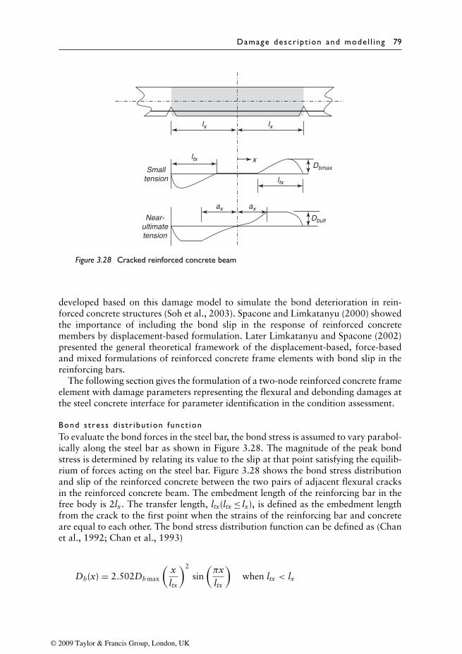
Damage descr ipt ion and mode l l ing 79
Smalltension
Dbmax
ltx
ltx
lx lx
Near-ultimatetension
x
ax ax
Dbult
Figure 3.28 Cracked reinforced concrete beam
developed based on this damage model to simulate the bond deterioration in rein-forced concrete structures (Soh et al., 2003). Spacone and Limkatanyu (2000) showedthe importance of including the bond slip in the response of reinforced concretemembers by displacement-based formulation. Later Limkatanyu and Spacone (2002)presented the general theoretical framework of the displacement-based, force-basedand mixed formulations of reinforced concrete frame elements with bond slip in thereinforcing bars.
The following section gives the formulation of a two-node reinforced concrete frameelement with damage parameters representing the flexural and debonding damages atthe steel concrete interface for parameter identification in the condition assessment.
Bond stress d i s tr ibut ion funct ionTo evaluate the bond forces in the steel bar, the bond stress is assumed to vary parabol-ically along the steel bar as shown in Figure 3.28. The magnitude of the peak bondstress is determined by relating its value to the slip at that point satisfying the equilib-rium of forces acting on the steel bar. Figure 3.28 shows the bond stress distributionand slip of the reinforced concrete between the two pairs of adjacent flexural cracksin the reinforced concrete beam. The embedment length of the reinforcing bar in thefree body is 2lx. The transfer length, ltx(ltx ≤ lx), is defined as the embedment lengthfrom the crack to the first point when the strains of the reinforcing bar and concreteare equal to each other. The bond stress distribution function can be defined as (Chanet al., 1992; Chan et al., 1993)
Db(x) = 2.502Db max
(xltx
)2
sin(πxltx
)when ltx < lx
© 2009 Taylor & Francis Group, London, UK
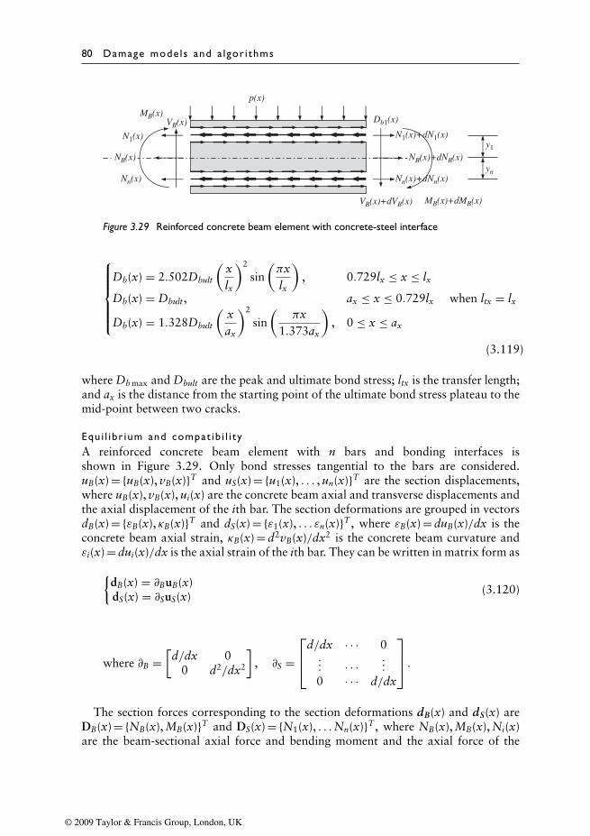
80 Damage mode ls and a lgor i thms
Nn(x)+dNn(x)
VB(x)+dVB(x) MB(x)+dMB(x)
MB(x)VB(x)
N1(x)+dN1(x)
Nn(x)
N1(x)y1
yn
Db1(x)
p(x)
NB(x)+dNB(x)NB(x)
Figure 3.29 Reinforced concrete beam element with concrete-steel interface
Db(x) = 2.502Dbult
(xlx
)2
sin(πxlx
), 0.729lx ≤ x ≤ lx
Db(x) = Dbult, ax ≤ x ≤ 0.729lx
Db(x) = 1.328Dbult
(xax
)2
sin(
πx1.373ax
), 0 ≤ x ≤ ax
when ltx = lx
(3.119)
where Db max and Dbult are the peak and ultimate bond stress; ltx is the transfer length;and ax is the distance from the starting point of the ultimate bond stress plateau to themid-point between two cracks.
Equ i l ibr ium and compat ib i l i t yA reinforced concrete beam element with n bars and bonding interfaces isshown in Figure 3.29. Only bond stresses tangential to the bars are considered.uB(x) = {uB(x), vB(x)}T and uS(x) = {u1(x), . . . , un(x)}T are the section displacements,where uB(x), vB(x), ui(x) are the concrete beam axial and transverse displacements andthe axial displacement of the ith bar. The section deformations are grouped in vectorsdB(x) = {εB(x), κB(x)}T and dS(x) = {ε1(x), . . . εn(x)}T , where εB(x) = duB(x)/dx is theconcrete beam axial strain, κB(x) = d2vB(x)/dx2 is the concrete beam curvature andεi(x) = dui(x)/dx is the axial strain of the ith bar. They can be written in matrix form as{
dB(x) = ∂BuB(x)dS(x) = ∂SuS(x)
(3.120)
where ∂B =[d/dx 0
0 d2/dx2
], ∂S =
d/dx · · · 0... · · · ...
0 · · · d/dx
.The section forces corresponding to the section deformations dB(x) and dS(x) are
DB(x) = {NB(x), MB(x)}T and DS(x) = {N1(x), . . .Nn(x)}T , where NB(x), MB(x), Ni(x)are the beam-sectional axial force and bending moment and the axial force of the
© 2009 Taylor & Francis Group, London, UK
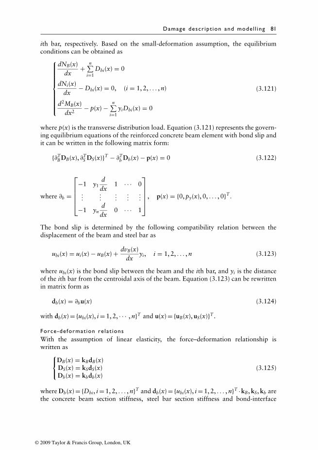
Damage descr ipt ion and mode l l ing 81
ith bar, respectively. Based on the small-deformation assumption, the equilibriumconditions can be obtained as
dNB(x)dx
+n∑
i=1Dbi(x) = 0
dNi(x)dx
− Dbi(x) = 0, (i = 1, 2, . . . , n)
d2MB(x)dx2
− p(x) −n∑
i=1yiDbi(x) = 0
(3.121)
where p(x) is the transverse distribution load. Equation (3.121) represents the govern-ing equilibrium equations of the reinforced concrete beam element with bond slip andit can be written in the following matrix form:
{∂TB DB(x), ∂TS DS(x)}T − ∂Tb Db(x) − p(x) = 0 (3.122)
where ∂b =
−1 y1
ddx
1 · · · 0...
............
−1 ynddx
0 · · · 1
, p(x) = {0, py(x), 0, . . . , 0}T .
The bond slip is determined by the following compatibility relation between thedisplacement of the beam and steel bar as
ubi(x) = ui(x) − uB(x) + dvB(x)dx
yi, i = 1, 2, . . . , n (3.123)
where ubi(x) is the bond slip between the beam and the ith bar, and yi is the distanceof the ith bar from the centroidal axis of the beam. Equation (3.123) can be rewrittenin matrix form as
db(x) = ∂bu(x) (3.124)
with db(x) = {ubi(x), i = 1, 2, · · · , n}T and u(x) = {uB(x), uS(x)}T .
Force-de format ion re la t ionsWith the assumption of linear elasticity, the force–deformation relationship iswritten as
DB(x) = kBdB(x)DS(x) = kSdS(x)Db(x) = kbdb(x)
(3.125)
where Db(x) = {Dbi, i = 1, 2, . . . , n}T and db(x) = {ubi(x), i = 1, 2, . . . , n}T ·kB, kS, kb arethe concrete beam section stiffness, steel bar section stiffness and bond-interface
© 2009 Taylor & Francis Group, London, UK
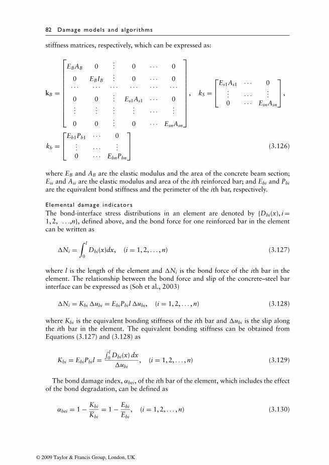
82 Damage mode ls and a lgor i thms
stiffness matrices, respectively, which can be expressed as:
kB =
EBAB 0... 0 · · · 0
0 EBIB... 0 · · · 0
· · · · · · · · · · · · · · · · · ·0 0
... Es1As1 · · · 0...
......
... · · · ...
0 0... 0 · · · EsnAsn
, kS =
Es1As1 · · · 0... · · · ...
0 · · · EsnAsn
,
kb =Eb1Pb1 · · · 0
... · · · ...
0 · · · EbnPbn
(3.126)
where EB and AB are the elastic modulus and the area of the concrete beam section;Esi and Asi are the elastic modulus and area of the ith reinforced bar; and Ebi and Pbi
are the equivalent bond stiffness and the perimeter of the ith bar, respectively.
E lementa l damage ind icatorsThe bond-interface stress distributions in an element are denoted by {Dbi(x), i =1, 2, . . .,n}, defined above, and the bond force for one reinforced bar in the elementcan be written as
�Ni =∫ l
0Dbi(x)dx, (i = 1, 2, . . . , n) (3.127)
where l is the length of the element and �Ni is the bond force of the ith bar in theelement. The relationship between the bond force and slip of the concrete–steel barinterface can be expressed as (Soh et al., 2003)
�Ni = Kbi�ubi = EbiPbil�ubi, (i = 1, 2, . . . , n) (3.128)
where Kbi is the equivalent bonding stiffness of the ith bar and �ubi is the slip alongthe ith bar in the element. The equivalent bonding stiffness can be obtained fromEquations (3.127) and (3.128) as
Kbi = EbiPbil =∫ l
0 Dbi(x) dx
�ubi, (i = 1, 2, . . . , n) (3.129)
The bond damage index, αbei, of the ith bar of the element, which includes the effectof the bond degradation, can be defined as
αbei = 1 − Kbi
Kbi
= 1 − Ebi
Ebi
, (i = 1, 2, . . . , n) (3.130)
© 2009 Taylor & Francis Group, London, UK
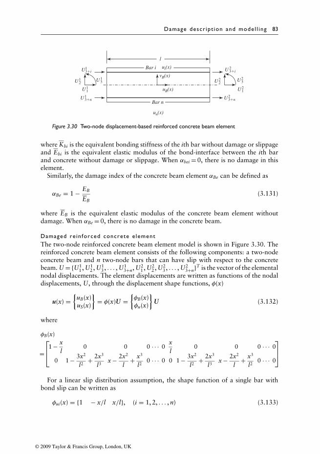
Damage descr ipt ion and mode l l ing 83
l
U13�i
Bar i
Bar n
U13U1
2
U11
U13�n
vB(x)
uB(x)
un(x)
ui(x) U 23�i
U23U2
2
U21
U23�n
Figure 3.30 Two-node displacement-based reinforced concrete beam element
where Kbi is the equivalent bonding stiffness of the ith bar without damage or slippageand Ebi is the equivalent elastic modulus of the bond-interface between the ith barand concrete without damage or slippage. When αbei = 0, there is no damage in thiselement.
Similarly, the damage index of the concrete beam element αBe can be defined as
αBe = 1 − EB
EB(3.131)
where EB is the equivalent elastic modulus of the concrete beam element withoutdamage. When αBe = 0, there is no damage in the concrete beam.
Damaged re in forced concrete e lementThe two-node reinforced concrete beam element model is shown in Figure 3.30. Thereinforced concrete beam element consists of the following components: a two-nodeconcrete beam and n two-node bars that can have slip with respect to the concretebeam. U = {U1
1 , U12 , U1
3 , . . . , U13+n, U2
1 , U22 , U2
3 , . . . , U23+n}T is the vector of the elemental
nodal displacements. The element displacements are written as functions of the nodaldisplacements, U, through the displacement shape functions, φ(x)
u(x) ={
uB(x)uS(x)
}= φ(x)U =
{φB(x)φu(x)
}U (3.132)
where
φB(x)
=1 − x
l0 0 0 · · · 0
xl
0 0 0 · · · 0
0 1 − 3x2
l2+ 2x3
l3x − 2x2
l+ x3
l20 · · · 0 0 1 − 3x2
l2+ 2x3
l3x − 2x2
l+ x3
l20 · · · 0
For a linear slip distribution assumption, the shape function of a single bar with
bond slip can be written as
φui(x) = {1 − x/l x/l}, (i = 1, 2, . . . , n) (3.133)
© 2009 Taylor & Francis Group, London, UK
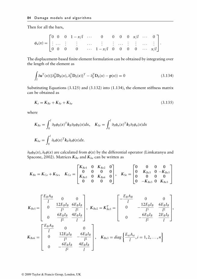
84 Damage mode ls and a lgor i thms
Then for all the bars,
φu(x) =0 0 0 1 − x/l · · · 0 0 0 0 x/l · · · 0... · · · ...
... · · · ...... · · · ...
... · · · ...
0 0 0 0 · · · 1 − x/l 0 0 0 0 · · · x/l
.The displacement-based finite element formulation can be obtained by integrating overthe length of the element as∫
lδuT (x)({∂TB DB(x), ∂TS DS(x)}T − ∂Tb Db(x) − p(x)) = 0 (3.134)
Substituting Equations (3.125) and (3.132) into (1.134), the element stiffness matrixcan be obtained as
K e = KBe + KSe + Kbe (3.135)
where
KBe =∫ l
0∂BφB(x)TkB∂BφB(x)dx, KSe =
∫ l
0∂Sφu(x)TkS∂Sφu(x)dx
Kbe =∫ l
0∂bφ(x)Tkb∂bφ(x)dx.
∂BφB(x), ∂bφ(x) are calculated from φ(x) by the differential operator (Limkatanyu andSpacone, 2002). Matrices KBe and Kbe can be written as
KBe = KCe + KSe, KCe =
KBe1 0 KBe2 0
0 0 0 0KBe5 0 KBe6 0
0 0 0 0
, KSe =
0 0 0 00 KBe3 0 −KBe3
0 0 0 00 −KBe3 0 KBe3
KBe1 =
EBAB
l0 0
012EBIB
l3
6EBIB
l2
06EBIB
l2
4EBIB
l
, KBe2 = KTBe5 =
−EBAB
l0 0
0 −12EBIB
l3
6EBIB
l2
0 −6EBIB
l2
2EBIB
l
,
KBe6 =
EBAB
l0 0
012EBIB
l3−6EBIB
l2
0 −6EBIB
l2
4EBIB
l
, KBe3 = diag{
EsiAsi
l, i = 1, 2, . . . , n
}
© 2009 Taylor & Francis Group, London, UK
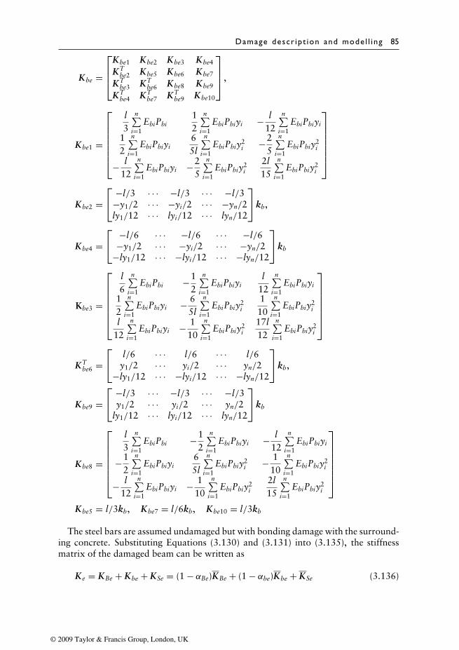
Damage descr ipt ion and mode l l ing 85
Kbe =
Kbe1 Kbe2 Kbe3 Kbe4
KTbe2 Kbe5 Kbe6 Kbe7
KTbe3 KT
be6 Kbe8 Kbe9
KTbe4 KT
be7 KTbe9 Kbe10
,
Kbe1 =
l3
n∑i=1
EbiPbi12
n∑i=1
EbiPbiyi − l12
n∑i=1
EbiPbiyi
12
n∑i=1
EbiPbiyi65l
n∑i=1
EbiPbiy2i −2
5
n∑i=1
EbiPbiy2i
− l12
n∑i=1
EbiPbiyi −25
n∑i=1
EbiPbiy2i
2l15
n∑i=1
EbiPbiy2i
Kbe2 = −l/3 · · · −l/3 · · · −l/3
−y1/2 · · · −yi/2 · · · −yn/2ly1/12 · · · lyi/12 · · · lyn/12
kb,
Kbe4 = −l/6 · · · −l/6 · · · −l/6
−y1/2 · · · −yi/2 · · · −yn/2−ly1/12 · · · −lyi/12 · · · −lyn/12
kb
Kbe3 =
l6
n∑i=1
EbiPbi −12
n∑i=1
EbiPbiyil
12
n∑i=1
EbiPbiyi
12
n∑i=1
EbiPbiyi − 65l
n∑i=1
EbiPbiy2i
110
n∑i=1
EbiPbiy2i
l12
n∑i=1
EbiPbiyi − 110
n∑i=1
EbiPbiy2i
17l12
n∑i=1
EbiPbiy2i
KTbe6 =
l/6 · · · l/6 · · · l/6y1/2 · · · yi/2 · · · yn/2
−ly1/12 · · · −lyi/12 · · · −lyn/12
kb,
Kbe9 = −l/3 · · · −l/3 · · · −l/3
y1/2 · · · yi/2 · · · yn/2ly1/12 · · · lyi/12 · · · lyn/12
kb
Kbe8 =
l3
n∑i=1
EbiPbi −12
n∑i=1
EbiPbiyi − l12
n∑i=1
EbiPbiyi
−12
n∑i=1
EbiPbiyi65l
n∑i=1
EbiPbiy2i − 1
10
n∑i=1
EbiPbiy2i
− l12
n∑i=1
EbiPbiyi − 110
n∑i=1
EbiPbiy2i
2l15
n∑i=1
EbiPbiy2i
Kbe5 = l/3kb, Kbe7 = l/6kb, Kbe10 = l/3kb
The steel bars are assumed undamaged but with bonding damage with the surround-ing concrete. Substituting Equations (3.130) and (3.131) into (3.135), the stiffnessmatrix of the damaged beam can be written as
K e = KBe + Kbe + KSe = (1 − αBe)KBe + (1 − αbe)Kbe + KSe (3.136)
© 2009 Taylor & Francis Group, London, UK
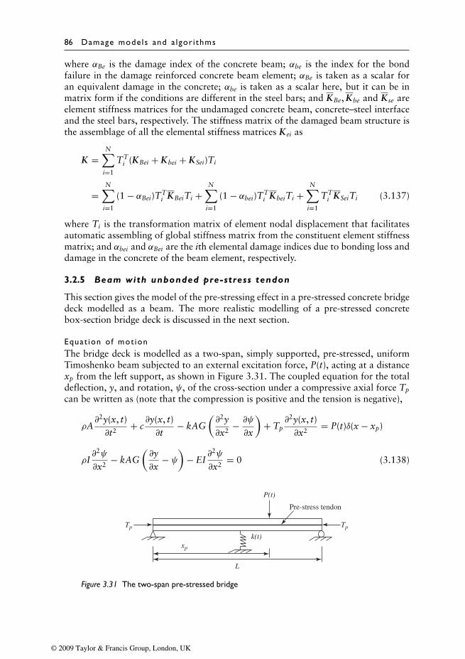
86 Damage mode ls and a lgor i thms
where αBe is the damage index of the concrete beam; αbe is the index for the bondfailure in the damage reinforced concrete beam element; αBe is taken as a scalar foran equivalent damage in the concrete; αbe is taken as a scalar here, but it can be inmatrix form if the conditions are different in the steel bars; and KBe, Kbe and K se areelement stiffness matrices for the undamaged concrete beam, concrete–steel interfaceand the steel bars, respectively. The stiffness matrix of the damaged beam structure isthe assemblage of all the elemental stiffness matrices K ei as
K =N∑
i=1
TTi (KBei + Kbei + KSei)Ti
=N∑
i=1
(1 − αBei)TTi KBeiTi +
N∑i=1
(1 − αbei)TTi KbeiTi +
N∑i=1
TTi KSeiTi (3.137)
where Ti is the transformation matrix of element nodal displacement that facilitatesautomatic assembling of global stiffness matrix from the constituent element stiffnessmatrix; and αbei and αBei are the ith elemental damage indices due to bonding loss anddamage in the concrete of the beam element, respectively.
3.2.5 Beam with unbonded pre-stress tendon
This section gives the model of the pre-stressing effect in a pre-stressed concrete bridgedeck modelled as a beam. The more realistic modelling of a pre-stressed concretebox-section bridge deck is discussed in the next section.
Equat ion of mot ionThe bridge deck is modelled as a two-span, simply supported, pre-stressed, uniformTimoshenko beam subjected to an external excitation force, P(t), acting at a distancexp from the left support, as shown in Figure 3.31. The coupled equation for the totaldeflection, y, and rotation, ψ, of the cross-section under a compressive axial force Tp
can be written as (note that the compression is positive and the tension is negative),
ρA∂2y(x, t)∂t2
+ c∂y(x, t)∂t
− kAG(∂2y∂x2
− ∂ψ∂x
)+ Tp
∂2y(x, t)∂x2
= P(t)δ(x − xp)
ρI∂2ψ
∂x2− kAG
(∂y∂x
− ψ)
− EI∂2ψ
∂x2= 0 (3.138)
L
TpTp
Pre-stress tendon
P(t)
xp
k(t)
Figure 3.31 The two-span pre-stressed bridge
© 2009 Taylor & Francis Group, London, UK
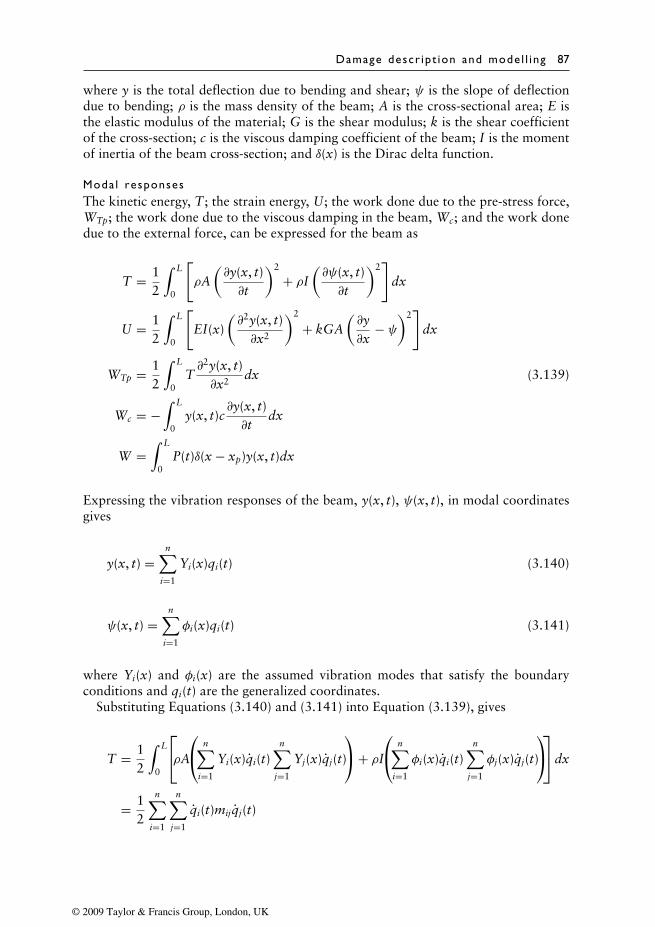
Damage descr ipt ion and mode l l ing 87
where y is the total deflection due to bending and shear; ψ is the slope of deflectiondue to bending; ρ is the mass density of the beam; A is the cross-sectional area; E isthe elastic modulus of the material; G is the shear modulus; k is the shear coefficientof the cross-section; c is the viscous damping coefficient of the beam; I is the momentof inertia of the beam cross-section; and δ(x) is the Dirac delta function.
Moda l responsesThe kinetic energy, T; the strain energy, U; the work done due to the pre-stress force,WTp; the work done due to the viscous damping in the beam, Wc; and the work donedue to the external force, can be expressed for the beam as
T = 12
∫ L
0
[ρA
(∂y(x, t)∂t
)2
+ ρI(∂ψ(x, t)∂t
)2]
dx
U = 12
∫ L
0
[EI(x)
(∂2y(x, t)∂x2
)2
+ kGA(∂y∂x
− ψ)2]
dx
WTp = 12
∫ L
0T∂2y(x, t)∂x2
dx (3.139)
Wc = −∫ L
0y(x, t)c
∂y(x, t)∂t
dx
W =∫ L
0P(t)δ(x − xp)y(x, t)dx
Expressing the vibration responses of the beam, y(x, t), ψ(x, t), in modal coordinatesgives
y(x, t) =n∑
i=1
Yi(x)qi(t) (3.140)
ψ(x, t) =n∑
i=1
φi(x)qi(t) (3.141)
where Yi(x) and φi(x) are the assumed vibration modes that satisfy the boundaryconditions and qi(t) are the generalized coordinates.
Substituting Equations (3.140) and (3.141) into Equation (3.139), gives
T = 12
∫ L
0
ρA n∑
i=1
Yi(x)qi(t)n∑
j=1
Yj(x)qj(t)
+ ρI n∑
i=1
φi(x)qi(t)n∑
j=1
φj(x)qj(t)
dx
= 12
n∑i=1
n∑j=1
qi(t)mijqj(t)
© 2009 Taylor & Francis Group, London, UK
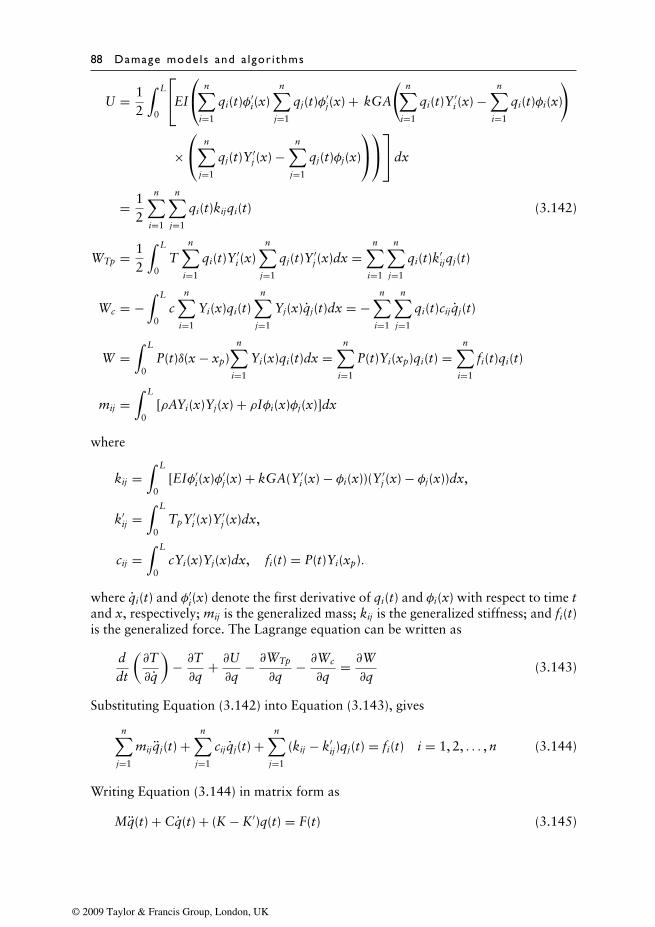
88 Damage mode ls and a lgor i thms
U = 12
∫ L
0
EI
n∑i=1
qi(t)φ′i(x)
n∑j=1
qj(t)φ′j(x) + kGA
(n∑
i=1
qi(t)Y ′i (x) −
n∑i=1
qi(t)φi(x)
)
× n∑
j=1
qj(t)Y ′j (x) −
n∑j=1
qj(t)φj(x)
dx
= 12
n∑i=1
n∑j=1
qi(t)kijqi(t) (3.142)
WTp = 12
∫ L
0T
n∑i=1
qi(t)Y ′i (x)
n∑j=1
qj(t)Y ′j (x)dx =
n∑i=1
n∑j=1
qi(t)k′ijqj(t)
Wc = −∫ L
0c
n∑i=1
Yi(x)qi(t)n∑
j=1
Yj(x)qj(t)dx = −n∑
i=1
n∑j=1
qi(t)cijqj(t)
W =∫ L
0P(t)δ(x − xp)
n∑i=1
Yi(x)qi(t)dx =n∑
i=1
P(t)Yi(xp)qi(t) =n∑
i=1
fi(t)qi(t)
mij =∫ L
0[ρAYi(x)Yj(x) + ρIφi(x)φj(x)]dx
where
kij =∫ L
0[EIφ′
i(x)φ′j(x) + kGA(Y ′
i (x) − φi(x))(Y ′j (x) − φj(x))dx,
k′ij =
∫ L
0TpY ′
i (x)Y ′j (x)dx,
cij =∫ L
0cYi(x)Yj(x)dx, fi(t) = P(t)Yi(xp).
where qi(t) and φ′i(x) denote the first derivative of qi(t) and φi(x) with respect to time t
and x, respectively; mij is the generalized mass; kij is the generalized stiffness; and fi(t)is the generalized force. The Lagrange equation can be written as
ddt
(∂T∂q
)− ∂T∂q
+ ∂U∂q
− ∂WTp
∂q− ∂Wc
∂q= ∂W∂q
(3.143)
Substituting Equation (3.142) into Equation (3.143), gives
n∑j=1
mijqj(t) +n∑
j=1
cijqj(t) +n∑
j=1
(kij − k′ij)qj(t) = fi(t) i = 1, 2, . . . , n (3.144)
Writing Equation (3.144) in matrix form as
Mq(t) + Cq(t) + (K − K′)q(t) = F(t) (3.145)
© 2009 Taylor & Francis Group, London, UK
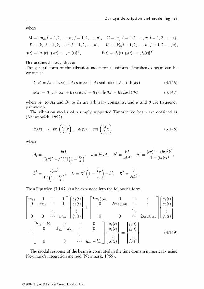
Damage descr ipt ion and mode l l ing 89
where
M = {mij, i = 1, 2, . . . , n; j = 1, 2, . . . , n}, C = {cij, i = 1, 2, . . . , n; j = 1, 2, . . . , n},K = {kij, i = 1, 2, . . .n; j = 1, 2, . . . , n}, K′ = {k′
ij, i = 1, 2, . . . , n; j = 1, 2, . . . , n},q(t) = {q1(t), q2(t), . . . , qn(t)}T , F(t) = {f1(t), f2(t), . . . , fn(t)}T
The assumed mode shapesThe general form of the vibration mode for a uniform Timoshenko beam can bewritten as
Y(x) = A1 cos(αx) + A2 sin(αx) + A3 sinh(βx) + A4 cosh(βx) (3.146)
φ(x) = B1 cos(αx) + B2 sin(αx) + B3 sinh(βx) + B4 cosh(βx) (3.147)
where A1 to A4 and B1 to B4 are arbitrary constants, and α and β are frequencyparameters.
The vibration modes of a simply supported Timoshenko beam are obtained as(Abramovich, 1992),
Yi(x) = Ai sin(
iπL
x)
, φi(x) = cos(
iπL
x)
(3.148)
where
Ai = iπL
[(iπ)2 − p2b2](1 − Tp
a
) , a = kGA, b2 = EIaL2
, p2 = (iπ)4 − (iπ)2k2
1 + (iπ)2D,
k2 = TpL2
EI(1 − Tp
a
) , D = R2(
1 − Tp
a
)+ b2, R2 = I
AL2
Then Equation (3.145) can be expanded into the following formm11 0 · · · 00 m22 · · · 0
. . .
0 0 · · · mnn
q1(t)q2(t)...
qn(t)
+
2m1ξ1ω1 0 · · · 0
0 2m2ξ2ω2 · · · 0. . .
0 0 · · · 2mnξnωn
q1(t)q2(t)...
qn(t)
+
k11 − k′
11 0 · · · 00 k22 − k′
22 · · · 0. . .
0 0 · · · knn − k′nn
q1(t)q2(t)...
qn(t)
=
f1(t)f2(t)...
fn(t)
(3.149)
The modal response of the beam is computed in the time domain numerically usingNewmark’s integration method (Newmark, 1959).
© 2009 Taylor & Francis Group, London, UK
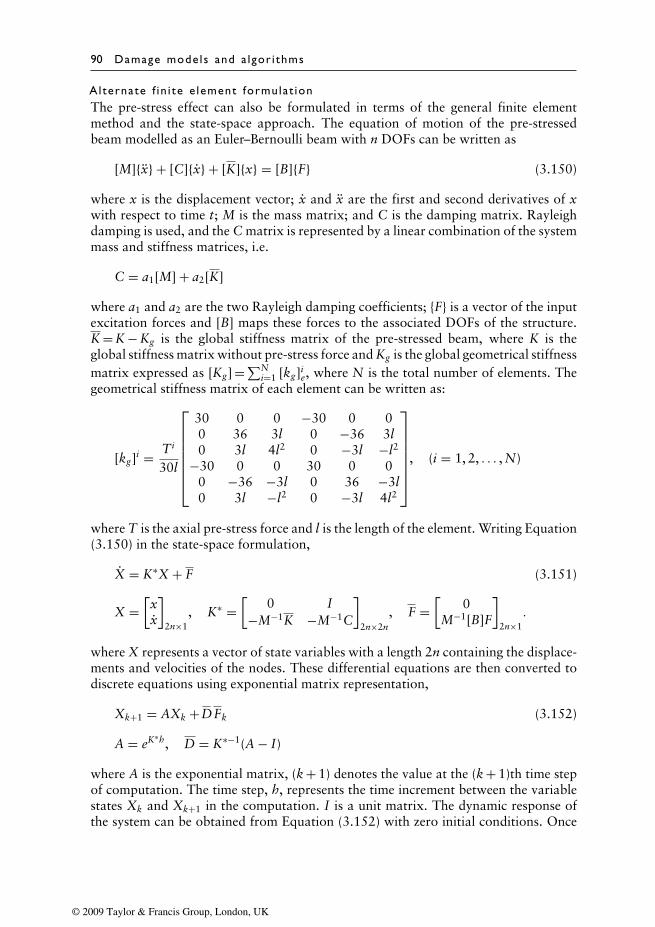
90 Damage mode ls and a lgor i thms
Al ternate f in i te e lement formula t ionThe pre-stress effect can also be formulated in terms of the general finite elementmethod and the state-space approach. The equation of motion of the pre-stressedbeam modelled as an Euler–Bernoulli beam with n DOFs can be written as
[M]{x} + [C]{x} + [K]{x} = [B]{F} (3.150)
where x is the displacement vector; x and x are the first and second derivatives of xwith respect to time t; M is the mass matrix; and C is the damping matrix. Rayleighdamping is used, and the C matrix is represented by a linear combination of the systemmass and stiffness matrices, i.e.
C = a1[M] + a2[K]
where a1 and a2 are the two Rayleigh damping coefficients; {F} is a vector of the inputexcitation forces and [B] maps these forces to the associated DOFs of the structure.K = K − Kg is the global stiffness matrix of the pre-stressed beam, where K is theglobal stiffness matrix without pre-stress force and Kg is the global geometrical stiffnessmatrix expressed as [Kg] =∑N
i=1 [kg]ie, where N is the total number of elements. The
geometrical stiffness matrix of each element can be written as:
[kg]i = Ti
30l
30 0 0 −30 0 00 36 3l 0 −36 3l0 3l 4l2 0 −3l −l2
−30 0 0 30 0 00 −36 −3l 0 36 −3l0 3l −l2 0 −3l 4l2
, (i = 1, 2, . . . , N)
where T is the axial pre-stress force and l is the length of the element. Writing Equation(3.150) in the state-space formulation,
X = K∗X + F (3.151)
X =[xx
]2n×1
, K∗ =[
0 I−M−1K −M−1C
]2n×2n
, F =[
0M−1[B]F
]2n×1.
where X represents a vector of state variables with a length 2n containing the displace-ments and velocities of the nodes. These differential equations are then converted todiscrete equations using exponential matrix representation,
Xk+1 = AXk +DFk (3.152)
A = eK∗h, D = K∗−1(A − I)
where A is the exponential matrix, (k + 1) denotes the value at the (k + 1)th time stepof computation. The time step, h, represents the time increment between the variablestates Xk and Xk+1 in the computation. I is a unit matrix. The dynamic response ofthe system can be obtained from Equation (3.152) with zero initial conditions. Once
© 2009 Taylor & Francis Group, London, UK
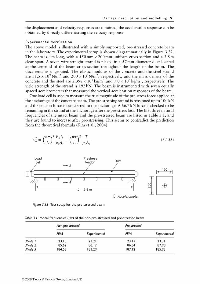
Damage descr ipt ion and mode l l ing 91
the displacement and velocity responses are obtained, the acceleration response can beobtained by directly differentiating the velocity response.
Exper imenta l ver i f i ca t ionThe above model is illustrated with a simply supported, pre-stressed concrete beamin the laboratory. The experimental setup is shown diagrammatically in Figure 3.32.The beam is 4 m long, with a 150 mm × 200 mm uniform cross-section and a 3.8 mclear span. A seven-wire straight strand is placed in a 57 mm diameter duct locatedat the centroid of the beam cross-section throughout the length of the beam. Theduct remains ungrouted. The elastic modulus of the concrete and the steel strandare 31.5 × 10⁹ N/m2 and 200 × 109N/m2, respectively, and the mass density of theconcrete and the steel are 2.398 × 10³ kg/m3 and 7.0 × 10³ kg/m3, respectively. Theyield strength of the strand is 192 kN. The beam is instrumented with seven equallyspaced accelerometers that measured the vertical acceleration responses of the beam.
One load cell is used to measure the true magnitude of the pre-stress force applied atthe anchorage of the concrete beam. The pre-stressing strand is tensioned up to 100 kNand the tension force is transferred to the anchorage. A 66.7 kN force is checked to beremaining in the strand at the anchorage after the pre-stress loss. The first three naturalfrequencies of the intact beam and the pre-stressed beam are listed in Table 3.1, andthey are found to increase after pre-stressing. This seems to contradict the predictionfrom the theoretical formula (Kim et al., 2004)
ω2n =
(nπL
)4 EbIb
ρcAc−(nπ
L
)2 TρcAc
(3.153)
Loadcell
Prestresstendon Duct
A
A
Accelerometer
L � 3.8 m
150
200
Figure 3.32 Test setup for the pre-stressed beam
Table 3.1 Modal frequencies (Hz) of the non-pre-stressed and pre-stressed beam
Non-pre-stressed Pre-stressed
FEM Experimental FEM Experimental
Mode 1 23.10 23.21 23.47 23.31Mode 2 85.62 86.17 86.54 87.98Mode 3 184.53 183.29 187.12 185.93
© 2009 Taylor & Francis Group, London, UK
92 Damage mode ls and a lgor i thms
where EbIb is equivalent to the flexural rigidity of the beam section; ρcAc is themass of the beam per unit length; and T is the magnitude of the pre-stress force.Equation (3.153) shows that an increase in the axial compressive force reduces themodal frequency and vice versa. But on further checking of the experimental system,the equivalent flexural rigidity of the beam without pre-stress force is found to be3.13 × 103 kN/m2, and it increases to 3.20 × 10³ kN/m2 after pre-stressing. Also, theequivalent mass per unit length of the beam is increased by 1.49% after pre-stressing.This is due to the presence of the additional equivalent flexural rigidity and the massof the pre-stressing strand. Thus, the physical presence of the pre-stressing tendon hasa dual effect on the natural frequency of the beam. The pre-stressing tendon itselfincreases the flexural rigidity and hence the natural frequency of the beam, but theself-weight and the compressive axial force it carries reduce the frequency of the beam.However, the stiffening effect from the increase in the equivalent flexural rigidity isgreater than the softening effect due to the compressive axial force and the additionalinertia effect due to its self-weight. And this results in a net increase in the naturalfrequency. The other effects, such as an increase in the dynamic modulus of concrete,are considered small and are therefore not discussed.
Ident i f i ca t ion of pre-s tress forceThe initial finite element model of the beam before pre-stressing consists of 16two-dimensional Euler–Bernoulli beam elements with three DOFs at each node. Animpulsive force is applied with the impact hammer at 1/4L from the left support of thebeam. The sampling rate is 2000 Hz. Time histories of both the excitation force and theacceleration are recorded, and data obtained from the third and fourth accelerometersare used in the model updating.
The support stiffnesses are updated using the response sensitivity approach (Lu andLaw, 2007a) with one second of measured data from the two accelerometers, andthe left and right support stiffnesses are updated to 8.9 × 10⁷ N/m and 9.4 × 10⁷ N/m,respectively. Rayleigh damping is adopted in calculating the structural response.
After the beam is pre-stressed, the pre-stress force is identified using the responsesensitivity approach described in Section 7.2 with data from 0.2 second to 1.0 secondafter the hammer impact. The first 0.2-second data is skipped because of the manyhigh frequency components in the response caused by the impulsive force created bythe hammer. An orthogonal polynomial function is used to remove the measurementnoise (Zhu and Law, 2001). The pre-stress force is identified using the penalty functionmethod (Mottershead and Friswell, 1993).
The identified pre-stress force and error are shown in Table 3.2, and they are veryclose to the true force, with a maximum error of 10.9% close to one end of thebeam. For convergence of the results, 56 iterations are required, and the correspond-ing optimal regularization parameter is 1.03 × 10⁻⁸. Figure 3.33 shows the curve ofconvergence, which indicates a clear converging characteristic, and Figure 3.34 showsthe reconstructed acceleration responses and the corresponding measured ones. It isnoted that these two sets of time histories match each other very well.
3.2.6 Pre-stressed concrete box-girder with bonded tendon
The bridge deck may lose some of its pre-stress force due to creep resulting from along period of service, under design or overloaded vehicles. A large reduction of the
© 2009 Taylor & Francis Group, London, UK
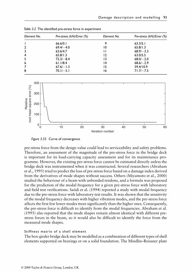
Damage descr ipt ion and mode l l ing 93
Table 3.2 The identified pre-stress force in experiment
Element No. Pre-stress (kN)/Error (%) Element No. Pre-stress (kN)/Error (%)
1 66.6/0.1 9 63.3/5.12 69.4/−4.0 10 65.8/1.33 63.6/4.7 11 68.9/−3.34 65.8/1.3 12 63.0/5.55 72.3/−8.4 13 68.0/−2.06 61.1/8.4 14 68.6/−2.97 67.6/−1.3 15 59.4/10.98 70.1/−5.1 16 71.7/−7.5
400
300
200
100
0
Rel
ativ
ero
ot m
ean
squa
re e
rror
(%
)
0 10 20 30 40 50 60Iteration number
Figure 3.33 Curve of convergence
pre-stress force from the design value could lead to serviceability and safety problems.Therefore, an assessment of the magnitude of the pre-stress force in the bridge deckis important for its load-carrying capacity assessment and for its maintenance pro-gramme. However, the existing pre-stress force cannot be estimated directly unless thebridge deck was instrumented when it was constructed. Several researchers (Abrahamet al., 1995) tried to predict the loss of pre-stress force based on a damage index derivedfrom the derivatives of mode shapes without success. Others (Miyamoto et al., 2000)studied the behaviour of a beam with unbonded tendons, and a formula was proposedfor the prediction of the modal frequency for a given pre-stress force with laboratoryand field test verifications. Saiidi et al. (1994) reported a study with modal frequencydue to the pre-stress force with laboratory test results. It was shown that the sensitivityof the modal frequency decreases with higher vibration modes, and the pre-stress forceaffects the first few lower modes more significantly than the higher ones. Consequently,the pre-stress force is difficult to identify from the modal frequencies. Abraham et al.(1995) also reported that the mode shapes remain almost identical with different pre-stress forces in the beam, so it would also be difficult to identify the force from themeasured mode shapes.
St i f fness matr ix o f a she l l e lementThe box-girder bridge deck may be modelled as a combination of different types of shellelements supported on bearings or on a solid foundation. The Mindlin–Reissner plate
© 2009 Taylor & Francis Group, London, UK
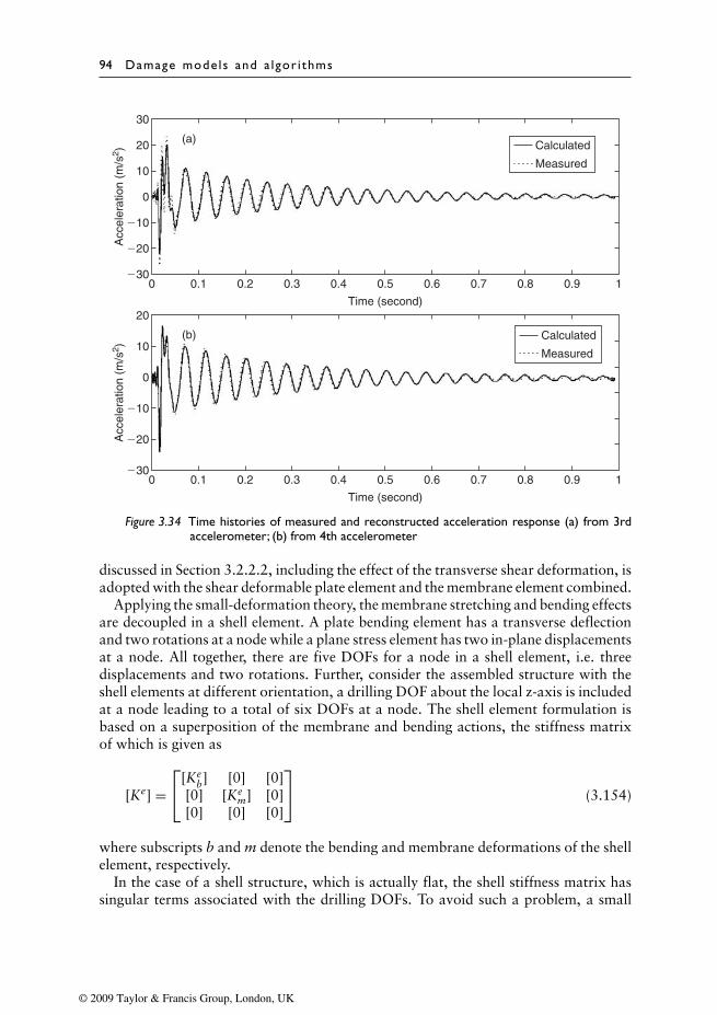
94 Damage mode ls and a lgor i thms
Calculated
Measured
30
20
10
0
�10
�20
�30
Acc
eler
atio
n (m
/s2 )
(a)
0 0.1 0.2 0.3 0.4 0.5 0.6 0.7 0.8 0.9 1
Time (second)20
10
0
�10
�20
�30
Acc
eler
atio
n (m
/s2 )
(b)
0 0.1 0.2 0.3 0.4 0.5 0.6 0.7 0.8 0.9 1
Time (second)
Calculated
Measured
Figure 3.34 Time histories of measured and reconstructed acceleration response (a) from 3rdaccelerometer; (b) from 4th accelerometer
discussed in Section 3.2.2.2, including the effect of the transverse shear deformation, isadopted with the shear deformable plate element and the membrane element combined.
Applying the small-deformation theory, the membrane stretching and bending effectsare decoupled in a shell element. A plate bending element has a transverse deflectionand two rotations at a node while a plane stress element has two in-plane displacementsat a node. All together, there are five DOFs for a node in a shell element, i.e. threedisplacements and two rotations. Further, consider the assembled structure with theshell elements at different orientation, a drilling DOF about the local z-axis is includedat a node leading to a total of six DOFs at a node. The shell element formulation isbased on a superposition of the membrane and bending actions, the stiffness matrixof which is given as
[Ke] =[Ke
b] [0] [0][0] [Ke
m] [0][0] [0] [0]
(3.154)
where subscripts b and m denote the bending and membrane deformations of the shellelement, respectively.
In the case of a shell structure, which is actually flat, the shell stiffness matrix hassingular terms associated with the drilling DOFs. To avoid such a problem, a small
© 2009 Taylor & Francis Group, London, UK

Damage descr ipt ion and mode l l ing 95
b1
a1
a2
b2
Concrete element
Pre-stressing tendon
Figure 3.35 Pre-stress tendon in a concrete element
number is added to the diagonal term of the matrix in Equation (3.154) associatedwith the drilling DOFs.
The pre-s tress ing tendonFigure 3.35 shows a segment of the pre-stressing tendon embedded into a flat shellelement. Noting that only the axial deformation of the tendon needs to be considered,the three-dimensional truss element is used to model the pre-stressing tendon.
The elemental stiffness of the tendon in terms of local coordinates is expressed as
[ke] = EsAs
l
1 0 0 −1 0 00 0 0 0 0 00 0 0 0 0 0
−1 0 0 1 0 00 0 0 0 0 00 0 0 0 0 0
(3.155)
The transformation matrix between the local and global coordinates system is given as
T =
ξ1 ξ2 ξ3η1 η2 η3 0ς1 ς2 ς3
ξ1 ξ2 ξ30 η1 η2 η3
ς1 ς2 ς3
(3.156)
where, {ξ1 η1 ς1} is the direction cosine of local x-axis with respect to the globalcoordinate system. Similarly, {ξ2 η2 ς2} and {ξ3 η3 ς3} are the direction cosinesof the local y-axis and z-axis with respect to the global coordinate system.
After transformation into the global coordinate system, the elemental stiffnessmatrix is expressed as
[ke] = [T]T [ke][T] (3.157)
Since [ke] is a 6 × 6 matrix and the elemental stiffness matrix of the shell element isof dimension 24 × 24, a transformation matrix is needed to expand matrix [ke] into a
© 2009 Taylor & Francis Group, London, UK
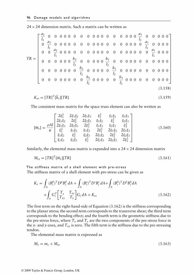
96 Damage mode ls and a lgor i thms
24 × 24 dimension matrix. Such a matrix can be written as
TR =
a2
l10 0 0 0 0 0 0 0 0 0 0 0 0 0 0 0 0
a1
l10 0 0 0 0
0a2
l10 0 0 0 0 0 0 0 0 0 0 0 0 0 0 0 0
a1
l10 0 0 0
0 0a2
l10 0 0 0 0 0 0 0 0 0 0 0 0 0 0 0 0
a1
l10 0 0
0 0 0 0 0 0b2
l20 0 0 0 0
b1
l20 0 0 0 0 0 0 0 0 0 0
0 0 0 0 0 0 0b2
l20 0 0 0 0
b1
l20 0 0 0 0 0 0 0 0 0
0 0 0 0 0 0 0 0b2
l20 0 0 0 0
b1
l20 0 0 0 0 0 0 0 0
(3.158)
Kes = [TR]T [ke][TR] (3.159)
The consistent mass matrix for the space truss element can also be written as
[me] = ρAl6
2ξ21 2ξ1ξ2 2ξ1ξ3 ξ21 ξ1ξ2 ξ1ξ32ξ1ξ2 2ξ22 2ξ2ξ3 ξ1ξ2 ξ22 ξ2ξ32ξ1ξ3 2ξ2ξ3 2ξ23 ξ1ξ3 ξ2ξ3 ξ23ξ21 ξ1ξ2 ξ1ξ3 2ξ21 2ξ1ξ2 2ξ1ξ3ξ1ξ2 ξ22 ξ2ξ3 2ξ1ξ2 2ξ22 2ξ2ξ3ξ1ξ3 ξ2ξ3 ξ23 2ξ1ξ3 2ξ2ξ3 2ξ23
(3.160)
Similarly, the elemental mass matrix is expanded into a 24 × 24 dimension matrix
Mes = [TR]T [me][TR] (3.161)
The st i f fness matr ix o f a she l l e lement wi th pre-s tressThe stiffness matrix of a shell element with pre-stress can be given as
Ke =∫
A(Bp
i )TDpBpj dA +
∫A
(Bsi )
TDsBsj dA+
∫A
(Bbi )TDbBb
j dA
+∫
AGT
i
[Tx Txy
Txy Ty
]Gj dA + Kes (3.162)
The first term on the right-hand-side of Equation (3.162) is the stiffness correspondingto the planar stress; the second term corresponds to the transverse shear; the third termcorresponds to the bending effect; and the fourth term is the geometric stiffness due tothe pre-stress force, where Tx and Ty are the two components of the pre-stress force inthe x- and y-axes, and Txy is zero. The fifth term is the stiffness due to the pre-stressingtendon.
The elemental mass matrix is expressed as
Me = me + Mes (3.163)
© 2009 Taylor & Francis Group, London, UK
Damage descr ipt ion and mode l l ing 97
The elemental matrices can then be assembled into the equation of motion for freevibration analysis and subsequent damage assessment.
3.2.7 Models with thin plate
Engineers have made many efforts to model crack-induced flexibility and investigateits effect on the dynamic characteristics of the damaged structure. Dimarogonas (1996)has summarized these works into three categories, namely: continuous model, discrete-continuous model and discrete models, i.e. finite-element models.
Real structures are more complicated than the geometrically simple ones describedby the first two types of models. Discrete models are usually used to study the crackedstructures – the finite element method (FEM) is the most popular and most commonlyused. A literature review of the FEM-based model of a cracked plate shows that thereare mainly three groups of methods. The simplest model represents the crack as areduction in the elasticity modulus of the element at the crack position (Cawley andAdams, 1979) or a reduction in the cross-sectional area of the element (Baschmid et al.,1984). These models have been successfully used in damage localization of plate-likestructures (Cornwell et al., 1999; Li et al., 2002). However, as these methods studythe approximate crack size and location at the element level, a very fine finite elementmesh is required to avoid a large error.
Another method models a crack by separating the nodes of finite elements alongthe crack line (Zastrau, 1985). To properly model the singular character of the stressand strain fields around the crack tip, a very dense mesh of finite elements or singular-shaped isoparametric elements (Shen and Pierre, 1990) are used to cover the cracktip area. Obviously, this method can model the cracked structure very well, but isnot suitable or feasible for damage identification. This is due to the low computationefficiency associated with the large number of finite element. Also, a finite elementmesh has to be constructed for each suspected location of damage in the plate at onetime.
In the third group of methods, a rectangular plate element with an open and depth-through crack parallel to the plate boundary is modelled (Qian et al., 1991; Krawczuk,1993; Krawczuk and Ostachowicz, 1994). The stiffness matrix of a cracked elementis written as K = TF−1TT , where F is the matrix representing the sum of the flexibilityof the non-cracked plate and the additional flexibility due to the crack; and T is atransformation matrix. However, as the derived stiffness matrix cannot be explicitlyparameterized in terms of damage variable(s) to indicate the location, orientation andthe extend of the crack, it is still difficult to incorporate this model into the inverseproblem of structural damage identification.
3.2.7.1 Anisot rop ic mode l o f e l l ip t i ca l c rack wi th s t ra in energy equ iva lence
The earliest crack model oriented towards damage identification was probably pre-sented by Lee et al. (1997). Although their work focuses on fracture mechanics andaims to derive a damage evolution equation that is consistent with the continuumdamage mechanics. Prior to this effort, there were a number of theories developed oncontinuum damage mechanics to derive the equivalent constitutive equation of a dam-aged material and its crack growth law on the basis of the strain equivalence principleintroduced by Lemaitre (1985) or the stress equivalence principle introduced by Simo
© 2009 Taylor & Francis Group, London, UK
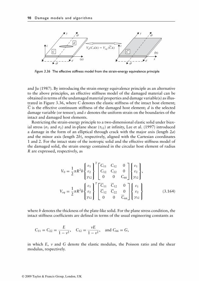
98 Damage mode ls and a lgor i thms
z
(a)
y
C
d
Vd(C,d,ε) � Veq (C,ε)
σ
σ
ε
z
(b)
y
x
C
σ
σ
ε
Figure 3.36 The effective stiffness model from the strain-energy equivalence principle
and Ju (1987). By introducing the strain energy equivalence principle as an alternativeto the above principles, an effective stiffness model of the damaged material can beobtained in terms of the undamaged material properties and damage variable(s) as illus-trated in Figure 3.36, where C denotes the elastic stiffness of the intact host element;C is the effective continuum stiffness of the damaged host element; d is the selecteddamage variable (or tensor); and ε denotes the uniform strain on the boundaries of theintact and damaged host elements.
Restricting the strain-energy principle to a two-dimensional elastic solid under biax-ial stress (σ1 and σ2) and in-plane shear (τ12) at infinity, Lee et al. (1997) introduceda damage in the form of an elliptical through crack with the major axis (length 2a)and the minor axis (length 2b), respectively, aligned with the Cartesian coordinates1 and 2. For the intact state of the isotropic solid and the effective stiffness model ofthe damaged solid, the strain energy contained in the circular host element of radiusR are expressed, respectively, as
V0 = 12πR2h
ε1
ε2
γ12
TC11 C12 0
C12 C22 00 0 C66
ε1
ε2
γ12
,
Veq = 12πR2h
ε1
ε2
γ12
TC11 C12 0
C12 C22 0
0 0 C66
ε1
ε2
γ12
(3.164)
where h denotes the thickness of the plate-like solid. For the plane stress condition, theintact stiffness coefficients are defined in terms of the usual engineering constants as
C11 = C22 = E1 − ν2
, C12 = νE1 − ν2
, and C66 = G,
in which E, ν and G denote the elastic modulus, the Poisson ratio and the shearmodulus, respectively.
© 2009 Taylor & Francis Group, London, UK
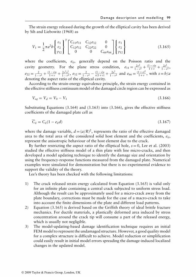
Damage descr ipt ion and mode l l ing 99
The strain energy released during the growth of the elliptical cavity has been derivedby Sih and Liebowitz (1968) as
V1 = 12πa2h
ε1ε2γ12
TC11e11 C12e12 0
C12e12 C22e22 00 0 C66e66
ε1ε2γ12
(3.165)
where the coefficients, eij, generally depend on the Poisson ratio and thecavity geometry. For the plane stress condition, e11 = 2ν2
1 − ν2 + (1 − ν)s1 + ν + 2s2
1 − ν2 ,
e22 = 21 − ν2 + (1 − ν)s
1 + ν + 2ν2s2
1 − ν2 , e12 = 21 − ν2 − (1 − ν)s
ν(1 + ν) + 2s2
1 − ν2 and e66 = (1 + s)2
1 + ν , with s = b/adenoting the aspect ratio of the elliptical cavity.
According to the strain-energy equivalence principle, the strain energy contained inthe effective stiffness continuum model of the damaged circle region can be expressed as
Veq = Vd = V0 − V1 (3.166)
Substituting Equations (3.164) and (3.165) into (3.166), gives the effective stiffnesscoefficients of the damaged plate cell as
Cij = Cij(1 − eijd) (3.167)
where the damage variable, d = (a/R)2, represents the ratio of the effective damagedarea to the total area of the considered solid host element and the coefficients, eij,represent the anisotropic behaviour of the host element due to the crack.
By further restricting the aspect ratio of the elliptical hole, s = 0, Lee et al. (2003)studied the effective stiffness model of a thin plate with line micro-cracks, and thendeveloped a model updating technique to identify the damage size and orientation byusing the frequency-response functions measured from the damaged plate. Numericalexamples were simulated for demonstration but there is no experimental evidence tosupport the validity of the theory.
Lee’s theory has been checked with the following limitations:
1) The crack released strain energy calculated from Equation (3.165) is valid onlyfor an infinite plate containing a central crack subjected to uniform stress load.Although the result can be approximately used for a micro-crack away from theplate boundary, corrections must be made for the case of a macro-crack to takeinto account the finite dimensions of the plate and different load patterns.
2) Equation (3.165) is derived based on the Griffith theory of ideal brittle fracturemechanics. For ductile materials, a plastically deformed area induced by stressconcentration around the crack tip will consume a part of the released energy,which is usually not negligible.
3) The model-updating-based damage identification technique requires an initialFEM model to represent the undamaged structure. However, a good quality modelfor a complex structure is difficult to achieve. Model reduction or simplificationcould easily result in initial model errors spreading the damage-induced localizedchanges in the updated model.
© 2009 Taylor & Francis Group, London, UK
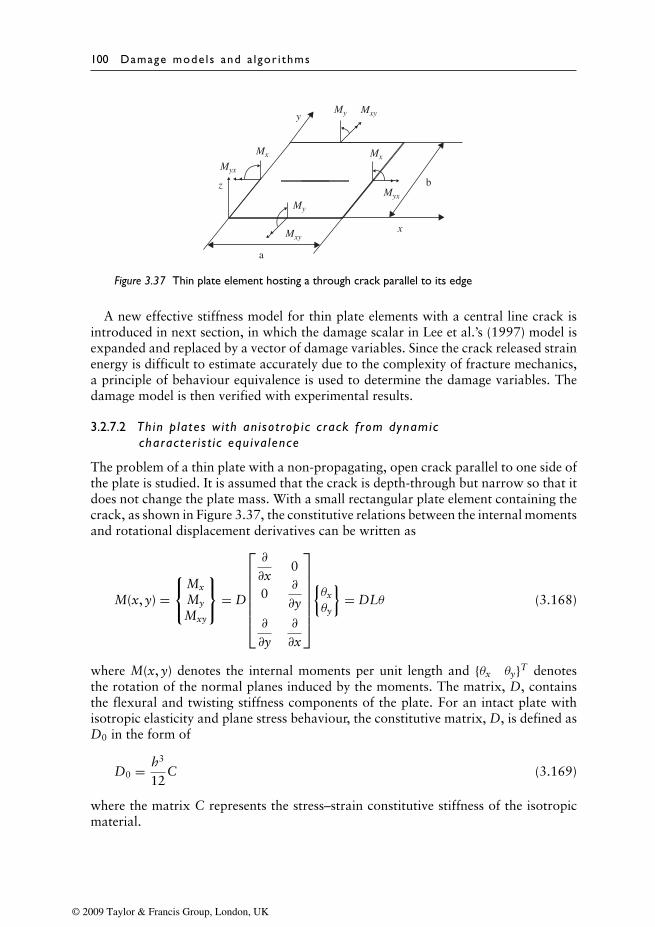
100 Damage mode ls and a lgor i thms
a
bz
x
yMxyMy
Myx
Mxy
Myx
My
Mx Mx
Figure 3.37 Thin plate element hosting a through crack parallel to its edge
A new effective stiffness model for thin plate elements with a central line crack isintroduced in next section, in which the damage scalar in Lee et al.’s (1997) model isexpanded and replaced by a vector of damage variables. Since the crack released strainenergy is difficult to estimate accurately due to the complexity of fracture mechanics,a principle of behaviour equivalence is used to determine the damage variables. Thedamage model is then verified with experimental results.
3.2.7.2 Thin p lates wi th an isot rop ic crack f rom dynamiccharacter i s t i c equ iva lence
The problem of a thin plate with a non-propagating, open crack parallel to one side ofthe plate is studied. It is assumed that the crack is depth-through but narrow so that itdoes not change the plate mass. With a small rectangular plate element containing thecrack, as shown in Figure 3.37, the constitutive relations between the internal momentsand rotational displacement derivatives can be written as
M(x, y) =
Mx
My
Mxy
= D
∂
∂x0
0∂
∂y
∂
∂y∂
∂x
{θxθy
}= DLθ (3.168)
where M(x, y) denotes the internal moments per unit length and {θx θy}T denotesthe rotation of the normal planes induced by the moments. The matrix, D, containsthe flexural and twisting stiffness components of the plate. For an intact plate withisotropic elasticity and plane stress behaviour, the constitutive matrix, D, is defined asD0 in the form of
D0 = h3
12C (3.169)
where the matrix C represents the stress–strain constitutive stiffness of the isotropicmaterial.
© 2009 Taylor & Francis Group, London, UK
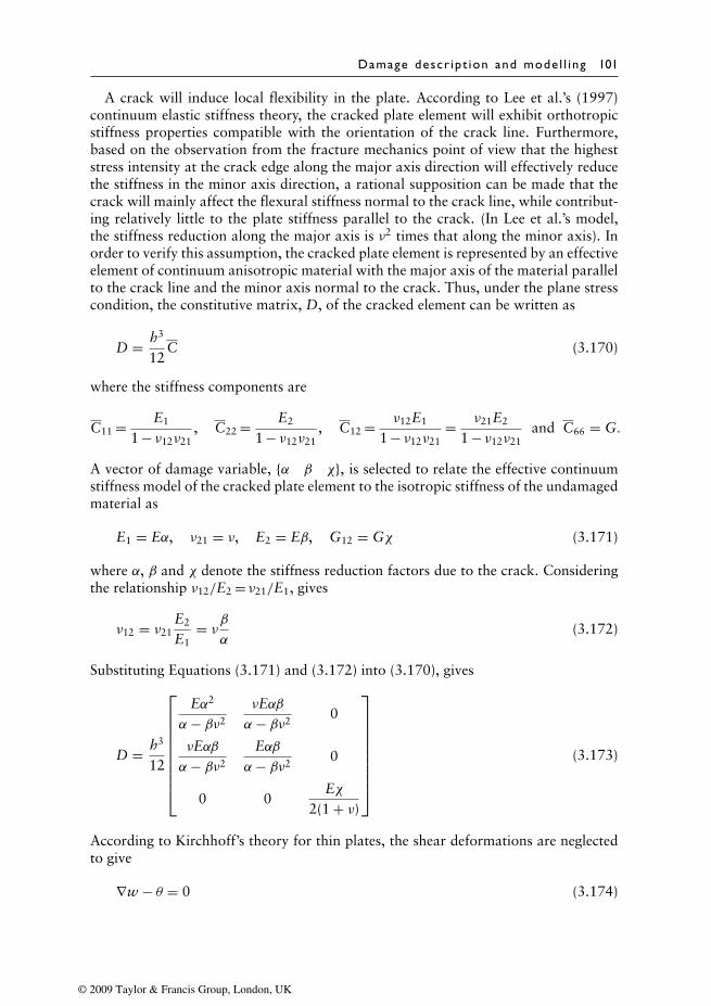
Damage descr ipt ion and mode l l ing 101
A crack will induce local flexibility in the plate. According to Lee et al.’s (1997)continuum elastic stiffness theory, the cracked plate element will exhibit orthotropicstiffness properties compatible with the orientation of the crack line. Furthermore,based on the observation from the fracture mechanics point of view that the higheststress intensity at the crack edge along the major axis direction will effectively reducethe stiffness in the minor axis direction, a rational supposition can be made that thecrack will mainly affect the flexural stiffness normal to the crack line, while contribut-ing relatively little to the plate stiffness parallel to the crack. (In Lee et al.’s model,the stiffness reduction along the major axis is ν2 times that along the minor axis). Inorder to verify this assumption, the cracked plate element is represented by an effectiveelement of continuum anisotropic material with the major axis of the material parallelto the crack line and the minor axis normal to the crack. Thus, under the plane stresscondition, the constitutive matrix, D, of the cracked element can be written as
D = h3
12C (3.170)
where the stiffness components are
C11 = E1
1 − ν12ν21, C22 = E2
1 − ν12ν21, C12 = ν12E1
1 − ν12ν21= ν21E2
1 − ν12ν21and C66 = G.
A vector of damage variable, {α β χ}, is selected to relate the effective continuumstiffness model of the cracked plate element to the isotropic stiffness of the undamagedmaterial as
E1 = Eα, ν21 = ν, E2 = Eβ, G12 = Gχ (3.171)
where α, β and χ denote the stiffness reduction factors due to the crack. Consideringthe relationship ν12/E2 = ν21/E1, gives
ν12 = ν21E2
E1= νβα
(3.172)
Substituting Equations (3.171) and (3.172) into (3.170), gives
D = h3
12
Eα2
α− βν2
νEαβα− βν2
0
νEαβα− βν2
Eαβα− βν2
0
0 0Eχ
2(1 + ν)
(3.173)
According to Kirchhoff’s theory for thin plates, the shear deformations are neglectedto give
∇w − θ = 0 (3.174)
© 2009 Taylor & Francis Group, London, UK
102 Damage mode ls and a lgor i thms
Substituting Equation (3.171) into Equation (3.164), gives
M(x, y) = Dκ(x, y) (3.175)
where the vector κ(x, y) ={∂2w∂x2
∂2w∂y2 2 ∂
2w∂x∂y
}= {κx κy κxy} contains the flexural
curvatures and twisting curvature at the middle plane of the plate.Now the transverse displacement function, w(x, y), can be defined as a biquadratic
polynomial
w(x, y) = pα (3.176)
where the vector p = {1 x y x2 xy y2 x3 x2y xy2 y3 x3y xy3}, andthe vector α= {α1 α2 · · · α12} denote the unknown coefficients. It is then conve-nient to express the deflection in terms of displacements at the four nodes of the plateelement as
w(x, y) = H(x, y)w (3.177)
where H(x, y) is the vector of isoparametric shape functions of the element, andw = {w1 w2 w3 w4 θx1 θx2 θx3 θx4 θy1 θy2 θy3 θy4} is the nodal dis-placement vector. Substituting Equation (3.177) into the constitutive relation inEquation (3.172) gives
M(x, y) = DB(x, y)w (3.178)
where B(x, y) =[∂2H∂x2 ; ∂2H
∂y2 ; 2 ∂2H∂x∂y
]. Equation (3.178) relates the internal moments
at any point of the element with the nodal displacements. The internal momentsat the four nodes are found by substituting the corresponding nodal coordinates,(xi, yi) i = 1 . . .4, into Equation (3.178). Writing this in matrix form gives{
MB
MT
}=[KBT KBR
KTT KTR
]{wT
wR
}= Kw (3.179)
where MB = {Mx1 My1 Mx2 My2 Mx3 My3 Mx4 My4}T denotes the bendingmoments at the four nodes; MT = {Mxy1 Mxy2 Mxy3 Mxy4}T denotes the nodaltwisting moments; wT = {w1 w2 w3 w4} denotes the translational DOFs at thefour nodes; and wR denotes the nodal rotational DOFs. Matrix K represents the generalconstitutive relations between the nodal loads and nodal displacements. RewritingEquation (3.179) in partitioned form, the rotational and translational displacementscan be expressed as
wR = K−1BRMB − K−1
BRKBTwT (3.180a)
wT = K∗TTMT − K∗
TTKTRwR (3.180b)
where the superscript * denotes the pseudo inverse of the matrix.To determine the coupled damage variables, {α β χ}, the above-mentioned princi-
ples of strain equivalence and strain energy equivalence do not work. They are extended
© 2009 Taylor & Francis Group, London, UK
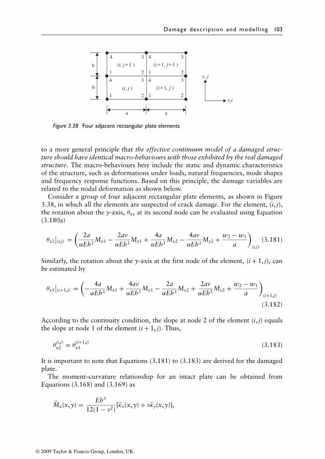
Damage descr ipt ion and mode l l ing 103
(i, j�1 ) (i�1, j�1 )
(i�1, j )(i, j )
x,i
y, j
a a
b
b
22
2
4 4
44
1
3
12
33
1
1
3
Figure 3.38 Four adjacent rectangular plate elements
to a more general principle that the effective continuum model of a damaged struc-ture should have identical macro-behaviours with those exhibited by the real damagedstructure. The macro-behaviours here include the static and dynamic characteristicsof the structure, such as deformations under loads, natural frequencies, mode shapesand frequency response functions. Based on this principle, the damage variables arerelated to the nodal deformation as shown below.
Consider a group of four adjacent rectangular plate elements, as shown in Figure3.38, in which all the elements are suspected of crack damage. For the element, (i, j),the rotation about the y-axis, θx, at its second node can be evaluated using Equation(3.180a)
θx2∣∣(i,j) =
(2aαEh3
Mx1 − 2aναEh3
My1 + 4aαEh3
Mx2 − 4aναEh3
My2 + w2 − w1
a
)(i,j)
(3.181)
Similarly, the rotation about the y-axis at the first node of the element, (i + 1, j), canbe estimated by
θx1∣∣(i+1,j) =
(− 4aαEh3
Mx1 + 4aναEh3
My1 − 2aαEh3
Mx2 + 2aναEh3
My2 + w2 − w1
a
)(i+1,j)
(3.182)
According to the continuity condition, the slope at node 2 of the element (i, j) equalsthe slope at node 1 of the element (i + 1, j). Thus,
θ(i,j)x2 = θ(i+1,j)
x1 (3.183)
It is important to note that Equations (3.181) to (3.183) are derived for the damagedplate.
The moment–curvature relationship for an intact plate can be obtained fromEquations (3.168) and (3.169) as
Mx(x, y) = Eh3
12(1 − ν2)[κx(x, y) + νκy(x, y)],
© 2009 Taylor & Francis Group, London, UK
104 Damage mode ls and a lgor i thms
My(x, y) = Eh3
12(1 − ν2)[κy(x, y) + νκx(x, y)] (3.184)
Mxy(x, y) = Eh3
12(1 + ν) κxy(x, y)
where the superscript ∼ denotes the terms for the intact plate. It is assumed thatthe applied loads only produce a small displacement in the plate structure, and thatthe additional displacement induced by the crack damage is also small, such that theinternal forces in the damaged structure can be approximately taken as those for theintact structure, which means Mx ≈ Mx, My ≈ My and Mxy ≈ Mxy. Therefore, Equation(3.184) can be directly substituted into Equations (3.181) to (3.183) to give(
κx1 + 2κx2
α
)(i,j)
+(
2κx1 + κx2
α
)(i+1,j)
= 6κ(i,j)x2 (3.185a)
Similarly, considering the slope continuity condition at node 3 of element (i, j) andnode 1 of element (i + 1, j), gives θ(i,j)x3 = θ(i+1,j)
x4 , yielding(κx4 + 2κx3
α
)(i,j)
+(
2κx4 + κx3
α
)(i+1,j)
= 6κ(i,j)x3 (3.185b)
Also, from the slope continuity condition of rotation, θy in the y-direction, θ(i,j)y4 = θ(i,j+1)y1
and θ(i,j)y3 = θ(i,j+1)y2 , leading to
(κy1 + 2κy4 + ν(κx1 + 2κx4)
β
)(i,j)
+(κy4 + 2κy1 + ν(κx4 + 2κx1)
β
)(i,j+1)
= 6(1 − ν2)κ(i,j)y4 + S14 (3.186a)
and (κy2 + 2κy3 + ν(κx2 + 2κx3)
β
)(i,j)
+(κy3 + 2κy2 + ν(κx3 + 2κx2)
β
)(i,j+1)
= 6(1 − ν2)κ(i,j)y3 + S23 (3.186b)
respectively, where
S14 =(ν(κx1 + 2κx4) + ν2(κy1 + 2κy4)
α
)(i,j)
+(ν(κx4 + 2κx1) + ν2(κy4 + 2κy1)
α
)(i,j+1)
,
S23 =(ν(κx2 + 2κx3) + ν2(κy2 + 2κy3)
α
)(i,j)
+(ν(κx3 + 2κx2) + ν2(κy3 + 2κy2)
α
)(i,j+1)
© 2009 Taylor & Francis Group, London, UK
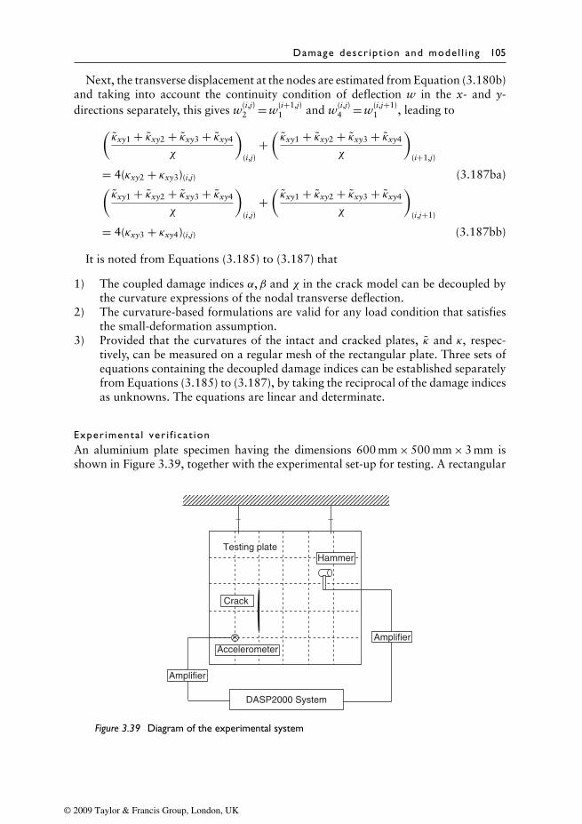
Damage descr ipt ion and mode l l ing 105
Next, the transverse displacement at the nodes are estimated from Equation (3.180b)and taking into account the continuity condition of deflection w in the x- and y-directions separately, this gives w(i,j)
2 = w(i+1,j)1 and w(i,j)
4 = w(i,j+1)1 , leading to(
κxy1 + κxy2 + κxy3 + κxy4
χ
)(i,j)
+(κxy1 + κxy2 + κxy3 + κxy4
χ
)(i+1,j)
= 4(κxy2 + κxy3)(i,j) (3.187ba)(κxy1 + κxy2 + κxy3 + κxy4
χ
)(i,j)
+(κxy1 + κxy2 + κxy3 + κxy4
χ
)(i,j+1)
= 4(κxy3 + κxy4)(i,j) (3.187bb)
It is noted from Equations (3.185) to (3.187) that
1) The coupled damage indices α,β and χ in the crack model can be decoupled bythe curvature expressions of the nodal transverse deflection.
2) The curvature-based formulations are valid for any load condition that satisfiesthe small-deformation assumption.
3) Provided that the curvatures of the intact and cracked plates, κ and κ, respec-tively, can be measured on a regular mesh of the rectangular plate. Three sets ofequations containing the decoupled damage indices can be established separatelyfrom Equations (3.185) to (3.187), by taking the reciprocal of the damage indicesas unknowns. The equations are linear and determinate.
Exper imenta l ver i f i ca t ionAn aluminium plate specimen having the dimensions 600 mm × 500 mm × 3 mm isshown in Figure 3.39, together with the experimental set-up for testing. A rectangular
∼∼
Hammer
Crack
Testing plate
AmplifierAccelerometer
DASP2000 System
Amplifier
Figure 3.39 Diagram of the experimental system
© 2009 Taylor & Francis Group, London, UK
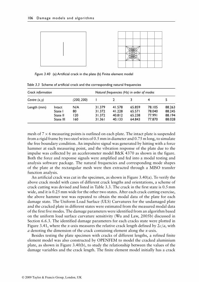
106 Damage mode ls and a lgor i thms
Figure 3.40 (a) Artificial crack in the plate (b) Finite element model
Table 3.3 Scheme of artificial crack and the corresponding natural frequencies
Crack information Natural frequencies (Hz) in order of modes
Centre (x, y) (200, 200) 1 2 3 4 5
Length (mm) Intact N/A 31.379 41.578 65.859 78.105 88.263State I 80 31.372 41.228 65.571 78.040 88.245State II 120 31.372 40.812 65.238 77.991 88.194State III 160 31.361 40.133 64.843 77.870 88.028
mesh of 7 × 6 measuring points is outlined on each plate. The intact plate is suspendedfrom a rigid frame by two steel wires of 0.5 mm in diameter and 0.75 m long, to simulatethe free boundary condition. An impulsive signal was generated by hitting with a forcehammer at each measuring point, and the vibration response of the plate due to theimpulse was collected by an accelerometer model B&K 4370 as shown in the figure.Both the force and response signals were amplified and fed into a modal testing andanalysis software package. The natural frequencies and corresponding mode shapesof the plate at the rectangular mesh were then extracted through a MISO transferfunction analysis.
An artificial crack was cut in the specimen, as shown in Figure 3.40(a). To verify theabove crack model with cases of different crack lengths and orientations, a scheme ofcrack cutting was devised and listed in Table 3.3. The crack in the first state is 0.5 mmwide, and it is 0.25 mm wide for the other two states. After each crack cutting exercise,the above hammer test was repeated to obtain the modal data of the plate for eachdamage state. The Uniform Load Surface (ULS) Curvatures for the undamaged plateand the cracked plate in different states were estimated from the measured modal dataof the first five modes. The damage parameters were identified from an algorithm basedon the uniform load surface curvature sensitivity (Wu and Law, 2005b) discussed inSection 6.6.3. The identified damage parameters for each cracks state were plotted inFigure 3.41, where the x-axis measures the relative crack length defined by 2c/a, witha denoting the dimension of the crack containing element along the x-axis.
Besides testing the plate specimen with cracks of different lengths, a refined finiteelement model was also constructed by OPENFEM to model the cracked aluminiumplate, as shown in Figure 3.40(b), to study the relationship between the values of thedamage variables and the crack length. The finite element model initially has a crack
© 2009 Taylor & Francis Group, London, UK
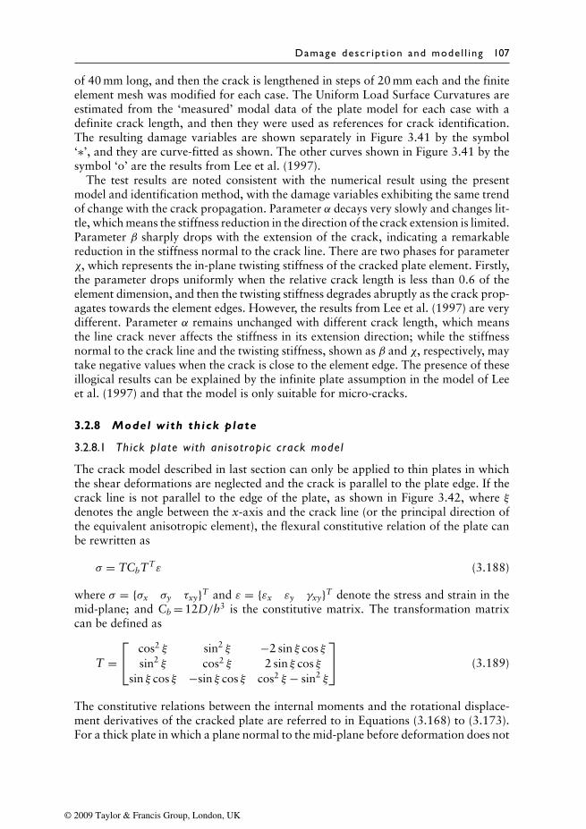
Damage descr ipt ion and mode l l ing 107
of 40 mm long, and then the crack is lengthened in steps of 20 mm each and the finiteelement mesh was modified for each case. The Uniform Load Surface Curvatures areestimated from the ‘measured’ modal data of the plate model for each case with adefinite crack length, and then they were used as references for crack identification.The resulting damage variables are shown separately in Figure 3.41 by the symbol‘∗’, and they are curve-fitted as shown. The other curves shown in Figure 3.41 by thesymbol ‘o’ are the results from Lee et al. (1997).
The test results are noted consistent with the numerical result using the presentmodel and identification method, with the damage variables exhibiting the same trendof change with the crack propagation. Parameter α decays very slowly and changes lit-tle, which means the stiffness reduction in the direction of the crack extension is limited.Parameter β sharply drops with the extension of the crack, indicating a remarkablereduction in the stiffness normal to the crack line. There are two phases for parameterχ, which represents the in-plane twisting stiffness of the cracked plate element. Firstly,the parameter drops uniformly when the relative crack length is less than 0.6 of theelement dimension, and then the twisting stiffness degrades abruptly as the crack prop-agates towards the element edges. However, the results from Lee et al. (1997) are verydifferent. Parameter α remains unchanged with different crack length, which meansthe line crack never affects the stiffness in its extension direction; while the stiffnessnormal to the crack line and the twisting stiffness, shown as β and χ, respectively, maytake negative values when the crack is close to the element edge. The presence of theseillogical results can be explained by the infinite plate assumption in the model of Leeet al. (1997) and that the model is only suitable for micro-cracks.
3.2.8 Model with thick plate
3.2.8.1 Thick p late wi th an isot rop ic crack mode l
The crack model described in last section can only be applied to thin plates in whichthe shear deformations are neglected and the crack is parallel to the plate edge. If thecrack line is not parallel to the edge of the plate, as shown in Figure 3.42, where ξdenotes the angle between the x-axis and the crack line (or the principal direction ofthe equivalent anisotropic element), the flexural constitutive relation of the plate canbe rewritten as
σ = TCbTTε (3.188)
where σ = {σx σy τxy}T and ε = {εx εy γxy}T denote the stress and strain in themid-plane; and Cb = 12D/h3 is the constitutive matrix. The transformation matrixcan be defined as
T = cos2 ξ sin2 ξ −2 sin ξ cos ξ
sin2 ξ cos2 ξ 2 sin ξ cos ξsin ξ cos ξ −sin ξ cos ξ cos2 ξ − sin2 ξ
(3.189)
The constitutive relations between the internal moments and the rotational displace-ment derivatives of the cracked plate are referred to in Equations (3.168) to (3.173).For a thick plate in which a plane normal to the mid-plane before deformation does not
© 2009 Taylor & Francis Group, London, UK
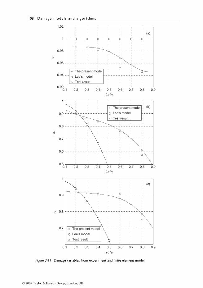
108 Damage mode ls and a lgor i thms
0.1 0.2 0.3 0.4 0.5 0.6 0.7 0.8 0.90.92
0.94
0.96
0.98
1
1.02
The present model
Lee's model
Test result
2c /a
α
0.1 0.2 0.3 0.4 0.5 0.6 0.7 0.8 0.90.5
0.6
0.7
0.8
0.9
1
2c /a
0.1 0.2 0.3 0.4 0.5 0.6 0.7 0.8 0.9
2c /a
β
0.7
0.8
0.9
1
χ
(a)
(b)
(c)
The present model
Lee's model
Test result
The present model
Lee's model
Test result
Figure 3.41 Damage variables from experiment and finite element model
© 2009 Taylor & Francis Group, London, UK
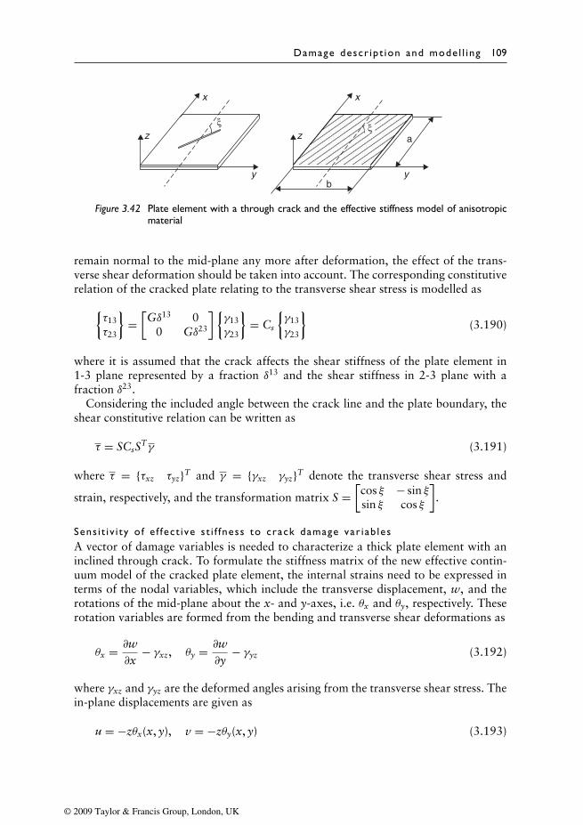
Damage descr ipt ion and mode l l ing 109
z
y
x
z
y
x
a
b
ξ ξ
Figure 3.42 Plate element with a through crack and the effective stiffness model of anisotropicmaterial
remain normal to the mid-plane any more after deformation, the effect of the trans-verse shear deformation should be taken into account. The corresponding constitutiverelation of the cracked plate relating to the transverse shear stress is modelled as{
τ13
τ23
}=[Gδ13 0
0 Gδ23
]{γ13
γ23
}= Cs
{γ13
γ23
}(3.190)
where it is assumed that the crack affects the shear stiffness of the plate element in1-3 plane represented by a fraction δ13 and the shear stiffness in 2-3 plane with afraction δ23.
Considering the included angle between the crack line and the plate boundary, theshear constitutive relation can be written as
τ = SCsSTγ (3.191)
where τ = {τxz τyz}T and γ = {γxz γyz}T denote the transverse shear stress and
strain, respectively, and the transformation matrix S =[cos ξ − sin ξsin ξ cos ξ
].
Sens i t i v i ty o f e f fect i ve s t i f fness to crack damage var iab lesA vector of damage variables is needed to characterize a thick plate element with aninclined through crack. To formulate the stiffness matrix of the new effective contin-uum model of the cracked plate element, the internal strains need to be expressed interms of the nodal variables, which include the transverse displacement, w, and therotations of the mid-plane about the x- and y-axes, i.e. θx and θy, respectively. Theserotation variables are formed from the bending and transverse shear deformations as
θx = ∂w∂x
− γxz, θy = ∂w∂y
− γyz (3.192)
where γxz and γyz are the deformed angles arising from the transverse shear stress. Thein-plane displacements are given as
u = −zθx(x, y), v = −zθy(x, y) (3.193)
© 2009 Taylor & Francis Group, London, UK
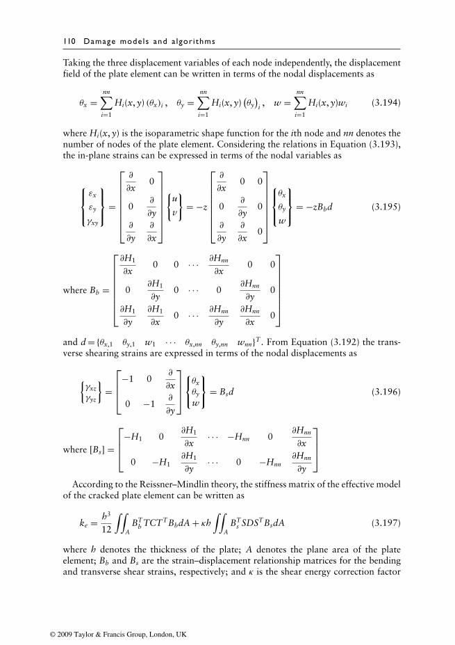
110 Damage mode ls and a lgor i thms
Taking the three displacement variables of each node independently, the displacementfield of the plate element can be written in terms of the nodal displacements as
θx =nn∑i=1
Hi(x, y) (θx)i , θy =nn∑i=1
Hi(x, y)(θy)
i , w =nn∑i=1
Hi(x, y)wi (3.194)
where Hi(x, y) is the isoparametric shape function for the ith node and nn denotes thenumber of nodes of the plate element. Considering the relations in Equation (3.193),the in-plane strains can be expressed in terms of the nodal variables as
εx
εy
γxy
=
∂
∂x0
0∂
∂y∂
∂y∂
∂x
{
u
v
}= −z
∂
∂x0 0
0∂
∂y0
∂
∂y∂
∂x0
θx
θy
w
= −zBbd (3.195)
where Bb =
∂H1
∂x0 0 · · · ∂Hnn
∂x0 0
0∂H1
∂y0 · · · 0
∂Hnn
∂y0
∂H1
∂y∂H1
∂x0 · · · ∂Hnn
∂y∂Hnn
∂x0
and d = {θx,1 θy,1 w1 · · · θx,nn θy,nn wnn}T . From Equation (3.192) the trans-verse shearing strains are expressed in terms of the nodal displacements as
{γxz
γyz
}=
−1 0∂
∂x
0 −1∂
∂y
θxθyw
= Bsd (3.196)
where [Bs] =
−H1 0∂H1
∂x· · · −Hnn 0
∂Hnn
∂x
0 −H1∂H1
∂y· · · 0 −Hnn
∂Hnn
∂y
According to the Reissner–Mindlin theory, the stiffness matrix of the effective model
of the cracked plate element can be written as
ke = h3
12
∫∫A
BTb TCTTBbdA + κh
∫∫A
BTs SDSTBsdA (3.197)
where h denotes the thickness of the plate; A denotes the plane area of the plateelement; Bb and Bs are the strain–displacement relationship matrices for the bendingand transverse shear strains, respectively; and κ is the shear energy correction factor
© 2009 Taylor & Francis Group, London, UK
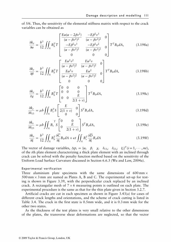
Damage descr ipt ion and mode l l ing 111
of 5/6. Thus, the sensitivity of the elemental stiffness matrix with respect to the crackvariables can be obtained as
∂ke
∂α= h3
12
∫∫A
BTb T
Eα(α− 2βν2)
(α− βν2)2
−Eβ2ν3
(α− βν2)20
−Eβ2ν3
(α− βν2)2
−Eβ2ν2
(α− βν2)20
0 0 0
TTBbdA, (3.198a)
∂ke
∂β= h3
12
∫∫A
BTb T
Eα2ν2
(α− βν2)2
Eα2ν
(α− βν2)20
Eα2ν
(α− βν2)2
Eα2
(α− βν2)20
0 0 0
TTBbdA, (3.198b)
∂ke
∂χ= h3
12
∫∫A
BTb T
0 0 00 0 0
0 0E
2(1 + ν)
TTBbdA, (3.198c)
∂ke
∂δ13= µh
∫∫A
BTs S
E2(1 + ν) 0
0 0
STBsdA, (3.198d)
∂ke
∂δ23= µh
∫∫A
Bs
T
S
0 0
0E
2(1 + ν)
STBsdA, (3.198e)
∂ke
∂ξ= h3
12
∫∫A
BTb
∂C∂ξ
BbdA + κt∫∫
ABT
s∂D∂ξ
BsdA (3.198f)
The vector of damage variables, �pi = {αi βi χi δ13,i δ23,i ξi}T (i = 1, · · · , ne),of the ith plate element characterizing a thick plate element with an inclined throughcrack can be solved with the penalty function method based on the sensitivity of theUniform Load Surface Curvature discussed in Section 6.6.3 (Wu and Law, 2004a).
Exper imenta l ver i f i ca t ionThree aluminium plate specimens with the same dimensions of 600 mm ×500 mm × 3 mm are named as Plates A, B and C. The experimental set-up for test-ing is shown in Figure 3.39, with the perpendicular crack replaced by an inclinedcrack. A rectangular mesh of 7 × 6 measuring points is outlined on each plate. Theexperimental procedure is the same as that for the thin plate given in Section 3.2.7.
Artificial cracks are cut in each specimen as shown in Figure 3.43(a) for cases ofdifferent crack lengths and orientations, and the scheme of crack cutting is listed inTable 3.4. The crack in the first state is 0.5mm wide, and it is 0.3 mm wide for theother two states.
As the thickness of the test plates is very small relative to the other dimensionsof the plates, the transverse shear deformations are neglected, so that the vector
© 2009 Taylor & Francis Group, London, UK
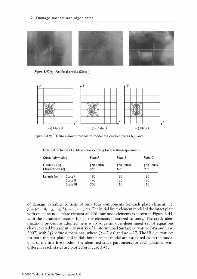
112 Damage mode ls and a lgor i thms
Figure 3.43(a) Artificial cracks (State I)
(a) Plate A (b) Plate B (c) Plate C
x
y
x
y
x
y
Figure 3.43(b) Finite element meshes to model the cracked plates A, B and C
Table 3.4 Scheme of artificial crack cutting for the three specimens
Crack information Plate A Plate B Plate C
Centre (x, y) (200,200) (200,200) (200,200)Orientation (ξ) 45◦ 60◦ 90◦
Length (mm) State I 80 80 80State II 140 120 120State III 200 160 160
of damage variables consists of only four components for each plate element, i.e.pi = {αi βi χi ξi}T (i = 1, · · · , ne). The initial finite element model of the intact platewith one nine-node plate element and 26 four-node elements is shown in Figure 3.44,with the parameter vectors for all the elements initialized to unity. The crack iden-tification procedure adopted here is to solve an over-determined set of equationscharacterized by a sensitivity matrix of Uniform Load Surface curvature (Wu and Law,2007) with 3Q × 4ne dimensions, where Q = 7 × 6 and ne = 27. The ULS curvaturesfor both the test plate and initial finite element model are estimated from the modaldata of the first five modes. The identified crack parameters for each specimen withdifferent crack states are plotted in Figure 3.45.
© 2009 Taylor & Francis Group, London, UK
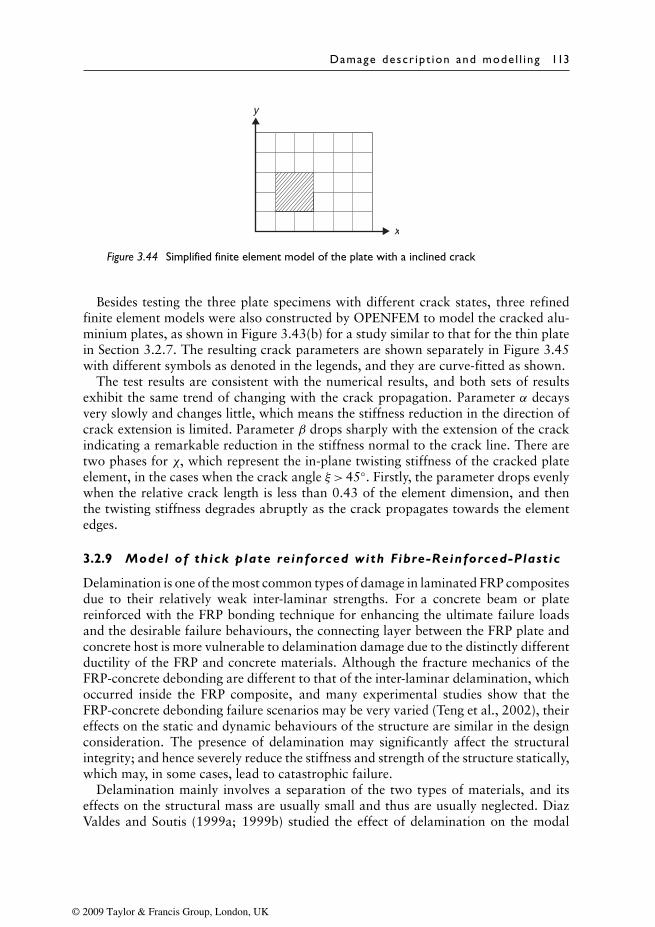
Damage descr ipt ion and mode l l ing 113
y
x
Figure 3.44 Simplified finite element model of the plate with a inclined crack
Besides testing the three plate specimens with different crack states, three refinedfinite element models were also constructed by OPENFEM to model the cracked alu-minium plates, as shown in Figure 3.43(b) for a study similar to that for the thin platein Section 3.2.7. The resulting crack parameters are shown separately in Figure 3.45with different symbols as denoted in the legends, and they are curve-fitted as shown.
The test results are consistent with the numerical results, and both sets of resultsexhibit the same trend of changing with the crack propagation. Parameter α decaysvery slowly and changes little, which means the stiffness reduction in the direction ofcrack extension is limited. Parameter β drops sharply with the extension of the crackindicating a remarkable reduction in the stiffness normal to the crack line. There aretwo phases for χ, which represent the in-plane twisting stiffness of the cracked plateelement, in the cases when the crack angle ξ >45◦. Firstly, the parameter drops evenlywhen the relative crack length is less than 0.43 of the element dimension, and thenthe twisting stiffness degrades abruptly as the crack propagates towards the elementedges.
3.2.9 Model of thick plate reinforced with Fibre-Reinforced-Plast ic
Delamination is one of the most common types of damage in laminated FRP compositesdue to their relatively weak inter-laminar strengths. For a concrete beam or platereinforced with the FRP bonding technique for enhancing the ultimate failure loadsand the desirable failure behaviours, the connecting layer between the FRP plate andconcrete host is more vulnerable to delamination damage due to the distinctly differentductility of the FRP and concrete materials. Although the fracture mechanics of theFRP-concrete debonding are different to that of the inter-laminar delamination, whichoccurred inside the FRP composite, and many experimental studies show that theFRP-concrete debonding failure scenarios may be very varied (Teng et al., 2002), theireffects on the static and dynamic behaviours of the structure are similar in the designconsideration. The presence of delamination may significantly affect the structuralintegrity; and hence severely reduce the stiffness and strength of the structure statically,which may, in some cases, lead to catastrophic failure.
Delamination mainly involves a separation of the two types of materials, and itseffects on the structural mass are usually small and thus are usually neglected. DiazValdes and Soutis (1999a; 1999b) studied the effect of delamination on the modal
© 2009 Taylor & Francis Group, London, UK
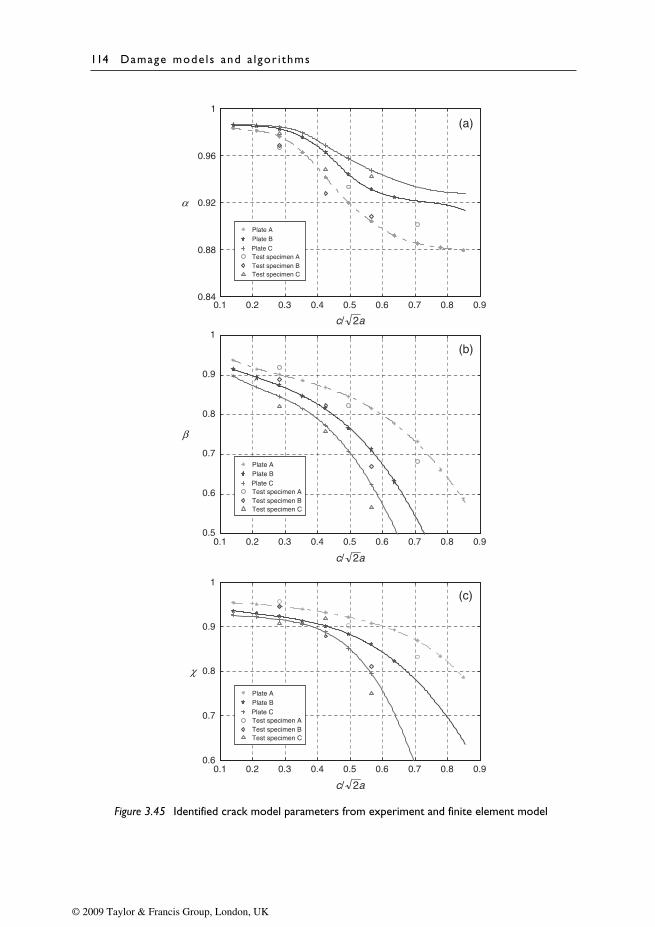
114 Damage mode ls and a lgor i thms
0.5
0.6
0.7
0.8
0.9
1
Plate APlate BPlate CTest specimen ATest specimen BTest specimen C
β
(b)
0.1 0.2 0.3 0.4 0.5 0.6 0.7 0.8 0.90.6
0.7
0.8
0.9
1
χ
c/ 2a
0.1 0.2 0.3 0.4 0.5 0.6 0.7 0.8 0.9
c/ 2a
c/ 2a
0.1 0.2 0.3 0.4 0.5 0.6 0.7 0.8 0.9
(c)
0.84
0.88
0.92
0.96
1
α
(a)
Plate A
Plate B
Plate CTest specimen ATest specimen BTest specimen C
Plate APlate BPlate CTest specimen ATest specimen BTest specimen C
Figure 3.45 Identified crack model parameters from experiment and finite element model
© 2009 Taylor & Francis Group, London, UK
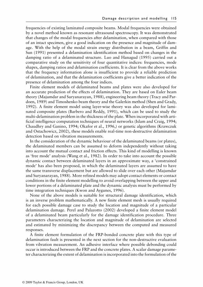
Damage descr ipt ion and mode l l ing 115
frequencies of existing laminated composite beams. Modal frequencies were obtainedby a novel method known as resonant ultrasound spectroscopy. It was demonstratedthat changes of the modal frequencies after delamination, when compared with thoseof an intact specimen, give a good indication on the presence and magnitude of dam-age. With the help of the modal strain energy distribution in a beam, Griffin andSun (1991) presented a delamination identification method based on changes in thedamping ratio of a delaminated structure. Luo and Hanagud (1995) carried out acomparative study on the sensitivity of four quantitative indices: frequencies, modeshapes, damping ratios and delamination coefficients. It is clear from the above worksthat the frequency information alone is insufficient to provide a reliable predictionof delamination, and that the delamination coefficients give a better indication of thepresence of delamination among the four indices.
Finite element models of delaminated beams and plates were also developed foran accurate prediction of the effects of delamination. They are based on Euler beamtheory (Majumdar and Suryanarayan, 1988), engineering beam theory (Tracy and Par-doen, 1989) and Timoshenko beam theory and the Galerkin method (Shen and Grady,1992). A finite element model using layer-wise theory was also developed for lami-nated composite plates (Barbero and Reddy, 1991), which can be used to study themulti-delamination problem in the thickness of the plate. When incorporated with arti-ficial intelligence computation techniques of neural networks (Islam and Craig, 1994;Chaudhry and Ganino, 1994; Okafor et al., 1996,) or genetic algorithms (Krawczukand Ostachowicz, 2002), these models enable real-time non-destructive delaminationdetection based on vibration measurements.
In the consideration of the dynamic behaviour of the delaminated beams (or plates),the delaminated members can be assumed to deform independently without takinginto account the mutual contact and friction effects. This kind of modelling is knownas ‘free mode’ analysis (Wang et al., 1982). In order to take into account the possibledynamic contact between delaminated layers in an approximate way, a ‘constrainedmode’ has also been proposed, in which the delaminated layers are assumed to havethe same transverse displacement but are allowed to slide over each other (Majumdarand Suryanarayan, 1988). More refined models may adopt contact elements or contactconditions in the finite element modelling to avoid overlapping between the upper andlower portions of a delaminated plate and the dynamic analysis must be performed bytime integration techniques (Kwon and Aygunes, 1996).
None of the above models is suitable for structural damage identification, whichis an inverse problem mathematically. A new finite element mesh is usually requiredfor each possible damage case to study the location and magnitude of a particulardelamination damage. Perel and Palazotto (2002) developed a finite element modelof a delaminated beam particularly for the damage identification procedure. Threeparameters characterizing the location and magnitude of delamination are selectedand estimated by minimizing the discrepancy between the computed and measuredresponses.
A finite element formulation of the FRP-bonded concrete plate with this type ofdelamination fault is presented in the next section for the non-destructive evaluationfrom vibration measurement. An adhesive interface where possible debonding couldoccur is introduced between the FRP and the concrete plates. A scalar damage parame-ter characterizing the extent of delamination is incorporated into the formulation of the
© 2009 Taylor & Francis Group, London, UK
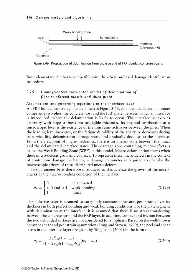
116 Damage mode ls and a lgor i thms
Bonded zone
Weak bonding zone
Concrete
FRP
Interface(thickness ≈ 0)
Figure 3.46 Propagation of delamination from the free end of FRP-bonded concrete beams
finite element model that is compatible with the vibration-based damage identificationprocedure.
3.2.9.1 Damage-detect ion-or iented mode l o f de laminat ion off ibre - re in forced p las t i c and th ick p late
Assumpt ions and govern ing equat ions o f the inter face layerAn FRP-bonded concrete plate, as shown in Figure 3.46, can be modelled as a laminatecomprising two plies: the concrete host and the FRP plate, between which an interfaceis introduced, where the delamination is likely to occur. The interface behaves asan entity with large stiffness but negligible thickness. Its physical justification at amicroscopic level is the existence of the thin resin-rich layer between the plies. Whenthe loading level increases, or the fatigue durability of the structure decreases duringits service life, delamination damage starts and gradually develops at the interface.From the viewpoint of micro-mechanics, there is an interim state between the intactand the delaminated interface states. This damage zone containing micro-defects iscalled the Weak Bonding Zone (WBZ) in this model. Macro delamination forms whenthese micro-defects grow and coalesce. To represent these micro-defects in the contextof continuum damage mechanics, a damage parameter is required to describe themacroscopic effects of these distributed micro-defects.
The parameter pb is therefore introduced to characterize the growth of the micro-cracks or the macro-bonding condition of the interface
pb =
0 delaminated> 0 and < 1 weak bonding1 intact
(3.199)
The adhesive layer is assumed to carry only constant shear and peel strains over itsthickness in both perfect bonding and weak bonding conditions. For the plate segmentwith delamination at the interface, it is assumed that there is no stress transferringbetween the concrete host and the FRP layer. In addition, contact and friction betweenthe two debonded surfaces are not considered for simplicity. Based on the well-knownconstant shear and peel strain assumption (Tong and Steven, 1999), the peel and shearstress in the interface layer are given by Tong et al. (2001) in the form of
σb = pbEad(1 − vad)(1 − 2vad)(1 + vad)had
(wf − wc) (3.200)
© 2009 Taylor & Francis Group, London, UK
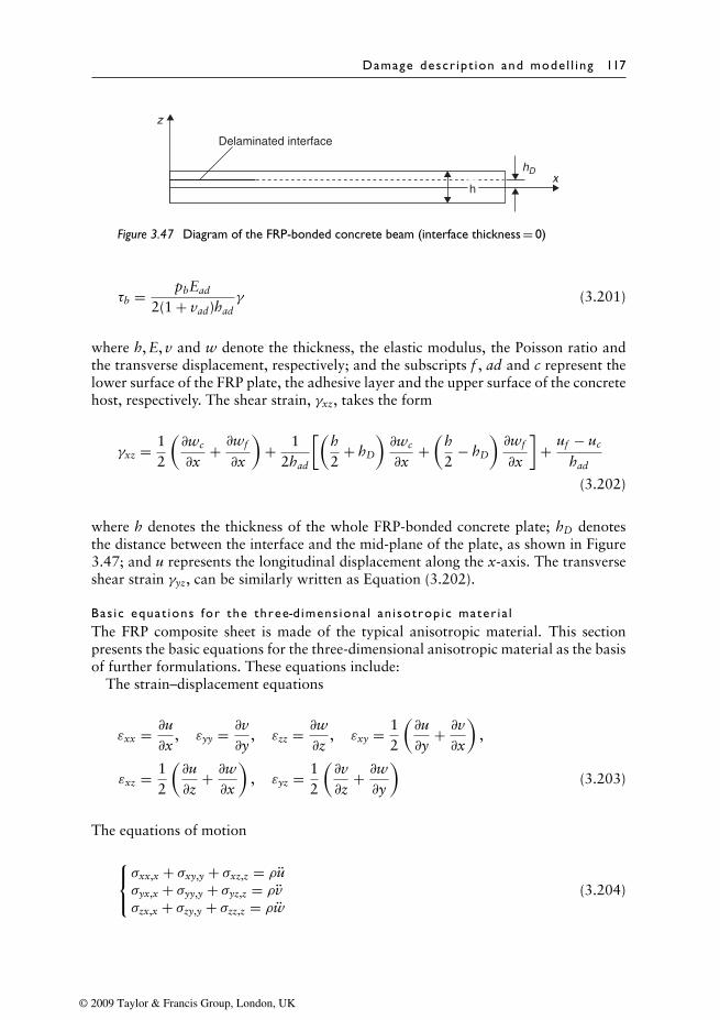
Damage descr ipt ion and mode l l ing 117
x
z
hD
Delaminated interface
h
Figure 3.47 Diagram of the FRP-bonded concrete beam (interface thickness = 0)
τb = pbEad
2(1 + vad)hadγ (3.201)
where h, E, v and w denote the thickness, the elastic modulus, the Poisson ratio andthe transverse displacement, respectively; and the subscripts f , ad and c represent thelower surface of the FRP plate, the adhesive layer and the upper surface of the concretehost, respectively. The shear strain, γxz, takes the form
γxz = 12
(∂wc
∂x+ ∂wf
∂x
)+ 1
2had
[(h2
+ hD
)∂wc
∂x+(
h2
− hD
)∂wf
∂x
]+ uf − uc
had
(3.202)
where h denotes the thickness of the whole FRP-bonded concrete plate; hD denotesthe distance between the interface and the mid-plane of the plate, as shown in Figure3.47; and u represents the longitudinal displacement along the x-axis. The transverseshear strain γyz, can be similarly written as Equation (3.202).
Bas ic equat ions for the three-d imens iona l an i sotrop ic mater ia lThe FRP composite sheet is made of the typical anisotropic material. This sectionpresents the basic equations for the three-dimensional anisotropic material as the basisof further formulations. These equations include:
The strain–displacement equations
εxx = ∂u∂x
, εyy = ∂v∂y
, εzz = ∂w∂z
, εxy = 12
(∂u∂y
+ ∂v∂x
),
εxz = 12
(∂u∂z
+ ∂w∂x
), εyz = 1
2
(∂v∂z
+ ∂w∂y
)(3.203)
The equations of motion
σxx,x + σxy,y + σxz,z = ρuσyx,x + σyy,y + σyz,z = ρvσzx,x + σzy,y + σzz,z = ρw
(3.204)
© 2009 Taylor & Francis Group, London, UK
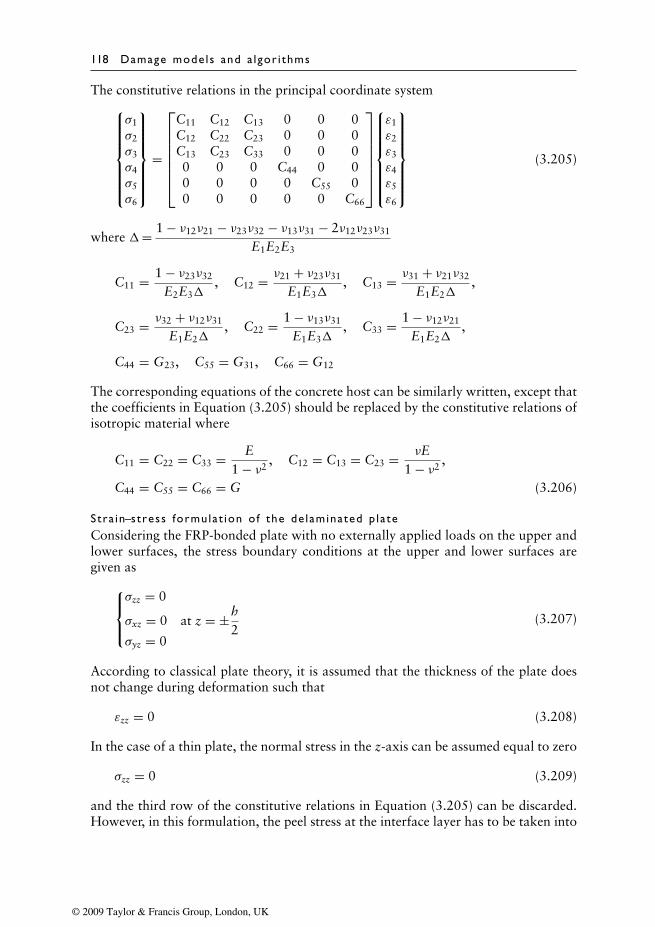
118 Damage mode ls and a lgor i thms
The constitutive relations in the principal coordinate system
σ1
σ2
σ3
σ4
σ5
σ6
=
C11 C12 C13 0 0 0C12 C22 C23 0 0 0C13 C23 C33 0 0 00 0 0 C44 0 00 0 0 0 C55 00 0 0 0 0 C66
ε1ε2ε3ε4ε5ε6
(3.205)
where �= 1 − ν12ν21 − ν23ν32 − ν13ν31 − 2ν12ν23ν31
E1E2E3
C11 = 1 − ν23ν32
E2E3�, C12 = ν21 + ν23ν31
E1E3�, C13 = ν31 + ν21ν32
E1E2�,
C23 = ν32 + ν12ν31
E1E2�, C22 = 1 − ν13ν31
E1E3�, C33 = 1 − ν12ν21
E1E2�,
C44 = G23, C55 = G31, C66 = G12
The corresponding equations of the concrete host can be similarly written, except thatthe coefficients in Equation (3.205) should be replaced by the constitutive relations ofisotropic material where
C11 = C22 = C33 = E1 − ν2
, C12 = C13 = C23 = νE1 − ν2
,
C44 = C55 = C66 = G (3.206)
Stra in–stress formula t ion of the de laminated p la teConsidering the FRP-bonded plate with no externally applied loads on the upper andlower surfaces, the stress boundary conditions at the upper and lower surfaces aregiven as
σzz = 0
σxz = 0 at z = ±h2
σyz = 0
(3.207)
According to classical plate theory, it is assumed that the thickness of the plate doesnot change during deformation such that
εzz = 0 (3.208)
In the case of a thin plate, the normal stress in the z-axis can be assumed equal to zero
σzz = 0 (3.209)
and the third row of the constitutive relations in Equation (3.205) can be discarded.However, in this formulation, the peel stress at the interface layer has to be taken into
© 2009 Taylor & Francis Group, London, UK
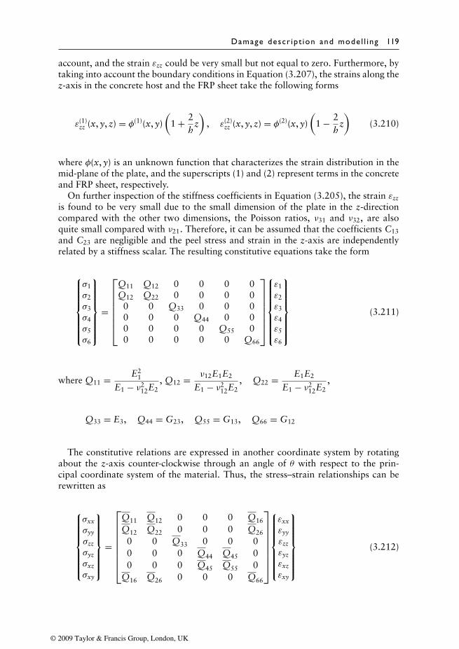
Damage descr ipt ion and mode l l ing 119
account, and the strain εzz could be very small but not equal to zero. Furthermore, bytaking into account the boundary conditions in Equation (3.207), the strains along thez-axis in the concrete host and the FRP sheet take the following forms
ε(1)zz (x, y, z) = φ(1)(x, y)
(1 + 2
hz)
, ε(2)zz (x, y, z) = φ(2)(x, y)
(1 − 2
hz)
(3.210)
where φ(x, y) is an unknown function that characterizes the strain distribution in themid-plane of the plate, and the superscripts (1) and (2) represent terms in the concreteand FRP sheet, respectively.
On further inspection of the stiffness coefficients in Equation (3.205), the strain εzz
is found to be very small due to the small dimension of the plate in the z-directioncompared with the other two dimensions, the Poisson ratios, ν31 and ν32, are alsoquite small compared with ν21. Therefore, it can be assumed that the coefficients C13
and C23 are negligible and the peel stress and strain in the z-axis are independentlyrelated by a stiffness scalar. The resulting constitutive equations take the form
σ1
σ2
σ3
σ4
σ5
σ6
=
Q11 Q12 0 0 0 0Q12 Q22 0 0 0 0
0 0 Q33 0 0 00 0 0 Q44 0 00 0 0 0 Q55 00 0 0 0 0 Q66
ε1ε2ε3ε4ε5ε6
(3.211)
where Q11 = E21
E1 − ν212E2
, Q12 = ν12E1E2
E1 − ν212E2
, Q22 = E1E2
E1 − ν212E2
,
Q33 = E3, Q44 = G23, Q55 = G13, Q66 = G12
The constitutive relations are expressed in another coordinate system by rotatingabout the z-axis counter-clockwise through an angle of θ with respect to the prin-cipal coordinate system of the material. Thus, the stress–strain relationships can berewritten as
σxx
σyy
σzz
σyz
σxz
σxy
=
Q11 Q12 0 0 0 Q16Q12 Q22 0 0 0 Q26
0 0 Q33 0 0 00 0 0 Q44 Q45 00 0 0 Q45 Q55 0
Q16 Q26 0 0 0 Q66
εxx
εyy
εzz
εyz
εxz
εxy
(3.212)
© 2009 Taylor & Francis Group, London, UK
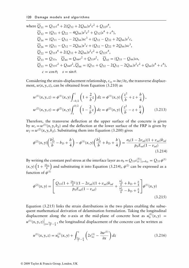
120 Damage mode ls and a lgor i thms
where Q11 = Q11c4 + 2(Q12 + 2Q66)s2c2 + Q22s4,
Q12 = (Q11 + Q22 − 4Q66)s2c2 + Q12(s4 + c4),
Q16 = (Q11 − Q12 − 2Q66)sc3 + (Q12 − Q22 + 2Q66)s3c,
Q26 = (Q11 − Q12 − 2Q66)s3c + (Q12 − Q22 + 2Q66)sc3,
Q22 = Q11s4 + 2(Q12 + 2Q66)s2c2 + Q22c4,
Q33 = Q33, Q44 = Q44c2 + Q55s2, Q45 = (Q55 − Q44)cs,
Q55 = Q55c2 + Q44s2, Q66 = (Q11 + Q22 − 2Q12 − 2Q66)s2c2 + Q66(s4 + c4),
c = cos θ; s = sin θ.
Considering the strain–displacement relationship, εzz = ∂w/∂z, the transverse displace-ment, w(x, y, z), can be obtained from Equation (3.210) as
w(1)(x, y, z) = φ(1)(x, y)∫ z
−h/2
(1 + 2
hz)
dz = φ(1)(x, y)(
z2
h+ z + h
4
),
w(2)(x, y, z) = φ(2)(x, y)∫ h/2
z
(1 − 2
hz)
dz = φ(2)(x, y)(
z2
h− z + h
4
)(3.213)
Therefore, the transverse deflection at the upper surface of the concrete is givenby wc = w(1)(x, y, hd) and the deflection at the lower surface of the FRP is given bywf = w(2)(x, y, hd). Substituting them into Equation (3.200) gives
φ(2)(x, y)(
h2D
h− hD + h
4
)− φ(1)(x, y)
(h2
D
h+ hD + h
4
)= σb(1 − 2vad)(1 + vad)had
pbEad(1 − vad)
(3.214)
By writing the constant peel stress at the interface layer as σb = Q33ε(1)zz∣∣z=hD = Q33φ
(1)
(x, y)(1 + 2hD
h
)and substituting it into Equation (3.214), φ(2) can be expressed as a
function of φ(1)
φ(2)(x, y) =Q33(1 + 2hD
h )(1 − 2vad)(1 + vad)had
pbEad(1 − vad)+
h2Dh + hD + h
4h2
Dh − hD + h
4
φ(1)(x, y)
(3.215)
Equation (3.215) links the strain distributions in the two plates enabling the subse-quent mathematical derivation of delamination formulation. Taking the longitudinaldisplacement along the x-axis at the mid-plane of concrete host as u(1)
0 (x, y) =u(1)(x, y, z)
∣∣∣z= hD
2 − h4
, the longitudinal displacement of the concrete can be written as
u(1)(x, y, z) = u(1)0 (x, y) +
∫ z
hD2 − h
4
(2ε(1)
xz − ∂w(1)
∂x
)dz (3.216)
© 2009 Taylor & Francis Group, London, UK
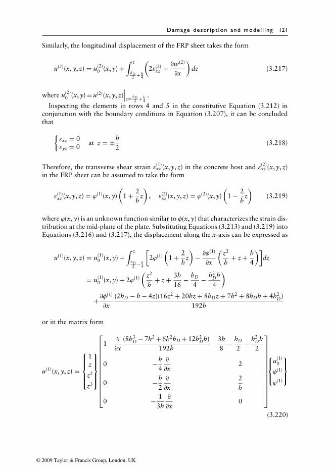
Damage descr ipt ion and mode l l ing 121
Similarly, the longitudinal displacement of the FRP sheet takes the form
u(2)(x, y, z) = u(2)0 (x, y) +
∫ z
hD2 + h
4
(2ε(2)
xz − ∂w(2)
∂x
)dz (3.217)
where u(2)0 (x, y) = u(2)(x, y, z)
∣∣∣z= hD
2 + h4
.
Inspecting the elements in rows 4 and 5 in the constitutive Equation (3.212) inconjunction with the boundary conditions in Equation (3.207), it can be concludedthat{
εxz = 0εyz = 0
at z = ±h2
(3.218)
Therefore, the transverse shear strain ε(1)xz (x, y, z) in the concrete host and ε(2)
xz (x, y, z)in the FRP sheet can be assumed to take the form
ε(1)xz (x, y, z) = ϕ(1)(x, y)
(1 + 2
hz)
, ε(2)xz (x, y, z) = ϕ(2)(x, y)
(1 − 2
hz)
(3.219)
where ϕ(x, y) is an unknown function similar to φ(x, y) that characterizes the strain dis-tribution at the mid-plane of the plate. Substituting Equations (3.213) and (3.219) intoEquations (3.216) and (3.217), the displacement along the x-axis can be expressed as
u(1)(x, y, z) = u(1)0 (x, y) +
∫ z
hD2 − h
4
[2ϕ(1)
(1 + 2
hz)
− ∂φ(1)
∂x
(z2
h+ z + h
4
)]dz
= u(1)0 (x, y) + 2ϕ(1)
(z2
h+ z + 3h
16− hD
4− h2
Dh4
)+∂φ
(1)
∂x(2hD − h − 4z)(16z2 + 20hz + 8hDz + 7h2 + 8hDh + 4h2
D)192h
or in the matrix form
u(1)(x, y, z) =
1z
z2
z3
1∂
∂x(8h3
D − 7h3 + 6h2hD + 12h2Dh)
192h3h8
− hD
2− h2
Dh2
0 −h4∂
∂x2
0 −h2∂
∂x2h
0 − 13h∂
∂x0
u(1)
0
φ(1)
ϕ(1)
(3.220)
© 2009 Taylor & Francis Group, London, UK
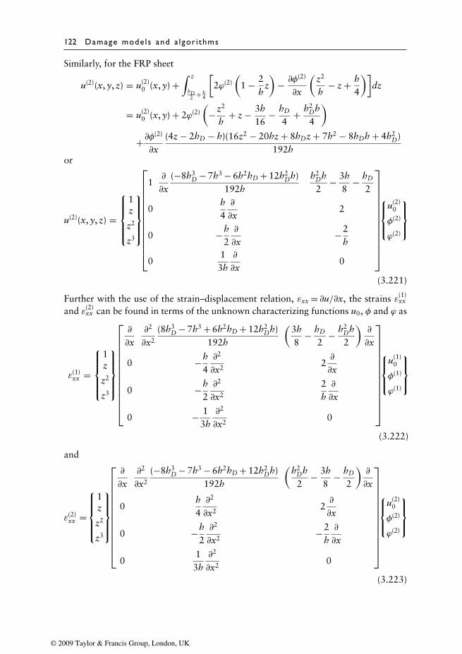
122 Damage mode ls and a lgor i thms
Similarly, for the FRP sheet
u(2)(x, y, z) = u(2)0 (x, y) +
∫ z
hD2 + h
4
[2ϕ(2)
(1 − 2
hz)
− ∂φ(2)
∂x
(z2
h− z + h
4
)]dz
= u(2)0 (x, y) + 2ϕ(2)
(−z2
h+ z − 3h
16− hD
4+ h2
Dh4
)+∂φ
(2)
∂x(4z − 2hD − h)(16z2 − 20hz + 8hDz + 7h2 − 8hDh + 4h2
D)192h
or
u(2)(x, y, z) =
1z
z2
z3
1∂
∂x(−8h3
D − 7h3 − 6h2hD + 12h2Dh)
192hh2
Dh2
− 3h8
− hD
2
0h4∂
∂x2
0 −h2∂
∂x−2
h
013h∂
∂x0
u(2)
0
φ(2)
ϕ(2)
(3.221)
Further with the use of the strain–displacement relation, εxx = ∂u/∂x, the strains ε(1)xx
and ε(2)xx can be found in terms of the unknown characterizing functions u0, φ and ϕ as
ε(1)xx =
1z
z2
z3
∂
∂x∂2
∂x2
(8h3D − 7h3 + 6h2hD + 12h2
Dh)192h
(3h8
− hD
2− h2
Dh2
)∂
∂x
0 −h4∂2
∂x22∂
∂x
0 −h2∂2
∂x2
2h∂
∂x
0 − 13h∂2
∂x20
u(1)
0
φ(1)
ϕ(1)
(3.222)
and
ε(2)xx =
1z
z2
z3
∂
∂x∂2
∂x2
(−8h3D − 7h3 − 6h2hD + 12h2
Dh)192h
(h2
Dh2
− 3h8
− hD
2
)∂
∂x
0h4∂2
∂x22∂
∂x
0 −h2∂2
∂x2−2
h∂
∂x
01
3h∂2
∂x20
u(2)
0
φ(2)
ϕ(2)
(3.223)
© 2009 Taylor & Francis Group, London, UK
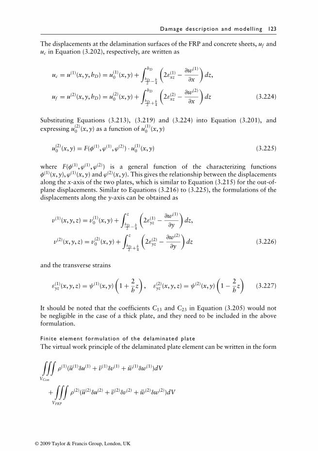
Damage descr ipt ion and mode l l ing 123
The displacements at the delamination surfaces of the FRP and concrete sheets, uf anduc in Equation (3.202), respectively, are written as
uc = u(1)(x, y, hD) = u(1)0 (x, y) +
∫ hD
hD2 − h
4
(2ε(1)
xz − ∂w(1)
∂x
)dz,
uf = u(2)(x, y, hD) = u(2)0 (x, y) +
∫ hD
hD2 + h
4
(2ε(2)
xz − ∂w(2)
∂x
)dz (3.224)
Substituting Equations (3.213), (3.219) and (3.224) into Equation (3.201), andexpressing u(2)
0 (x, y) as a function of u(1)0 (x, y)
u(2)0 (x, y) = F(φ(1),ϕ(1),ϕ(2)) · u(1)
0 (x, y) (3.225)
where F(φ(1),ϕ(1),ϕ(2)) is a general function of the characterizing functionsφ(1)(x, y),ϕ(1)(x, y) and ϕ(2)(x, y). This gives the relationship between the displacementsalong the x-axis of the two plates, which is similar to Equation (3.215) for the out-of-plane displacements. Similar to Equations (3.216) to (3.225), the formulations of thedisplacements along the y-axis can be obtained as
v(1)(x, y, z) = v(1)0 (x, y) +
∫ z
hD2 − h
4
(2ε(1)
yz − ∂w(1)
∂y
)dz,
v(2)(x, y, z) = v(2)0 (x, y) +
∫ z
hD2 + h
4
(2ε(2)
yz − ∂w(2)
∂y
)dz (3.226)
and the transverse strains
ε(1)yz (x, y, z) = ψ(1)(x, y)
(1 + 2
hz)
, ε(2)yz (x, y, z) = ψ(2)(x, y)
(1 − 2
hz)
(3.227)
It should be noted that the coefficients C13 and C23 in Equation (3.205) would notbe negligible in the case of a thick plate, and they need to be included in the aboveformulation.
F in i te e lement formula t ion of the de laminated p la teThe virtual work principle of the delaminated plate element can be written in the form
∫∫∫VCon
ρ(1)(u(1)δu(1) + v(1)δv(1) + w(1)δw(1))dV
+∫∫∫
VFRP
ρ(2)(u(2)δu(2) + v(2)δv(2) + w(2)δw(2))dV
© 2009 Taylor & Francis Group, London, UK
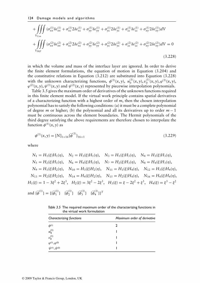
124 Damage mode ls and a lgor i thms
+∫∫∫
VCon
(σ(1)xx δε
(1)xx + σ(1)
xz 2δε(1)xz + σ(1)
yy δε(1)yy + σ(1)
yz 2δε(1)yz + σ(1)
zz δε(1)zz + σ(1)
xy 2δε(1)xy )dV
+∫∫∫
VFRP
(σ(2)xx δε
(2)xx + σ(2)
xz 2δε(2)xz + σ(2)
yy δε(2)yy + σ(2)
yz 2δε(2)yz + σ(2)
zz δε(2)zz + σ(2)
xy 2δε(2)xy )dV = 0
(3.228)
in which the volume and mass of the interface layer are ignored. In order to derivethe finite element formulations, the equation of motion in Equation (3.204) andthe constitutive relations in Equation (3.212) are substituted into Equation (3.228)with the unknown characterizing functions, φ(1)(x, y), u(1)
0 (x, y), v(1)0 (x, y),ϕ(1)(x, y),
ϕ(2)(x, y),ψ(1)(x, y) and ψ(2)(x, y) represented by piecewise interpolation polynomials.Table 3.5 gives the maximum order of derivatives of the unknown functions required
in this finite element model. If the virtual work principle contains spatial derivativesof a characterizing function with a highest order of m, then the chosen interpolationpolynomial has to satisfy the following conditions: (a) it must be a complete polynomialof degree m or higher; (b) the polynomial and all its derivatives up to order m − 1must be continuous across the element boundaries. The Hermit polynomials of thethird degree satisfying the above requirements are therefore chosen to interpolate thefunction φ(1)(x, y) as
φ(1)(x, y) = [N]1×16{φ(1)}16×1 (3.229)
where
N1 = H1(ξ)H1(η), N2 = H3(ξ)H1(η), N3 = H1(ξ)H3(η), N4 = H3(ξ)H3(η),
N5 = H2(ξ)H1(η), N6 = H4(ξ)H1(η), N7 = H2(ξ)H3(η), N8 = H4(ξ)H3(η),
N9 = H1(ξ)H2(η), N10 = H3(ξ)H2(η), N11 = H1(ξ)H4(η), N12 = H3(ξ)H4(η),
N13 = H2(ξ)H2(η), N14 = H4(ξ)H2(η), N15 = H2(ξ)H4(η), N16 = H4(ξ)H4(η),
H1(ξ) = 1 − 3ξ2 + 2ξ3, H2(ξ) = 3ξ2 − 2ξ3, H3(ξ) = ξ − 2ξ2 + ξ3, H4(ξ) = ξ3 − ξ2
and {φ(1)} = {{φ(1)1 } {φ(1)
2 } {φ(1)3 } {φ(1)
4 }}T
Table 3.5 The required maximum order of the characterizing functions inthe virtual work formulation
Characterizing functions Maximum order of derivative
φ(1) 2
u(1)0 1
v(1)0 1ϕ(1) ,ϕ(2) 1ψ(1) ,ψ(2) 1
© 2009 Taylor & Francis Group, London, UK
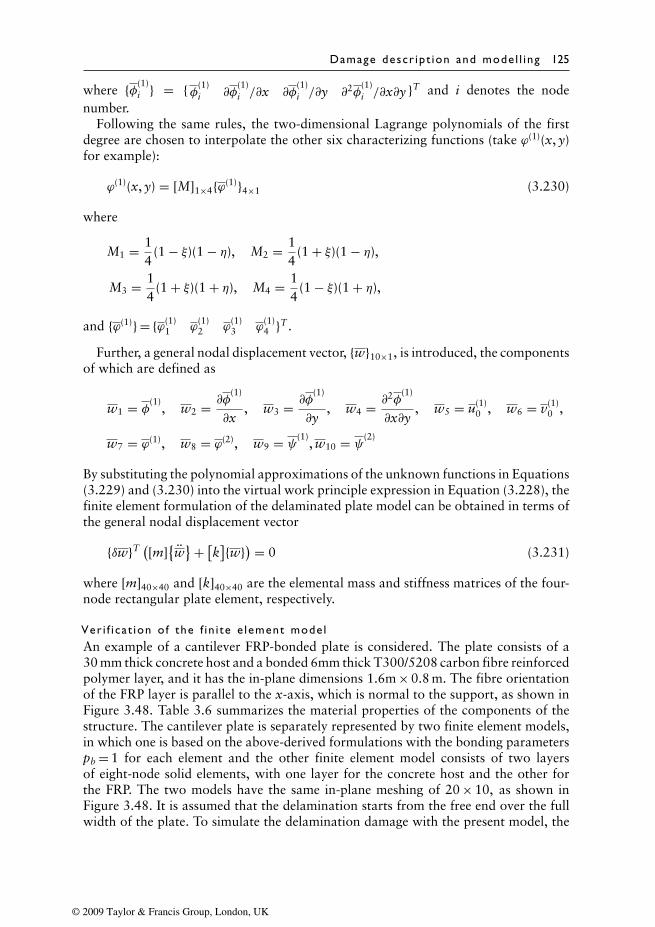
Damage descr ipt ion and mode l l ing 125
where {φ(1)i } = {φ(1)
i ∂φ(1)i /∂x ∂φ
(1)i /∂y ∂2φ
(1)i /∂x∂y }T and i denotes the node
number.Following the same rules, the two-dimensional Lagrange polynomials of the first
degree are chosen to interpolate the other six characterizing functions (take ϕ(1)(x, y)for example):
ϕ(1)(x, y) = [M]1×4{ϕ(1)}4×1 (3.230)
where
M1 = 14
(1 − ξ)(1 − η), M2 = 14
(1 + ξ)(1 − η),
M3 = 14
(1 + ξ)(1 + η), M4 = 14
(1 − ξ)(1 + η),
and {ϕ(1)} = {ϕ(1)1 ϕ
(1)2 ϕ
(1)3 ϕ
(1)4 }T .
Further, a general nodal displacement vector, {w}10×1, is introduced, the componentsof which are defined as
w1 = φ(1), w2 = ∂φ
(1)
∂x, w3 = ∂φ
(1)
∂y, w4 = ∂
2φ(1)
∂x∂y, w5 = u(1)
0 , w6 = v(1)0 ,
w7 = ϕ(1), w8 = ϕ(2), w9 = ψ(1), w10 = ψ(2)
By substituting the polynomial approximations of the unknown functions in Equations(3.229) and (3.230) into the virtual work principle expression in Equation (3.228), thefinite element formulation of the delaminated plate model can be obtained in terms ofthe general nodal displacement vector
{δw}T ([m]{w}+ [
k]{w}) = 0 (3.231)
where [m]40×40 and [k]40×40 are the elemental mass and stiffness matrices of the four-node rectangular plate element, respectively.
Ver i f i ca t ion of the f in i te e lement mode lAn example of a cantilever FRP-bonded plate is considered. The plate consists of a30 mm thick concrete host and a bonded 6mm thick T300/5208 carbon fibre reinforcedpolymer layer, and it has the in-plane dimensions 1.6m × 0.8 m. The fibre orientationof the FRP layer is parallel to the x-axis, which is normal to the support, as shown inFigure 3.48. Table 3.6 summarizes the material properties of the components of thestructure. The cantilever plate is separately represented by two finite element models,in which one is based on the above-derived formulations with the bonding parameterspb = 1 for each element and the other finite element model consists of two layersof eight-node solid elements, with one layer for the concrete host and the other forthe FRP. The two models have the same in-plane meshing of 20 × 10, as shown inFigure 3.48. It is assumed that the delamination starts from the free end over the fullwidth of the plate. To simulate the delamination damage with the present model, the
© 2009 Taylor & Francis Group, London, UK
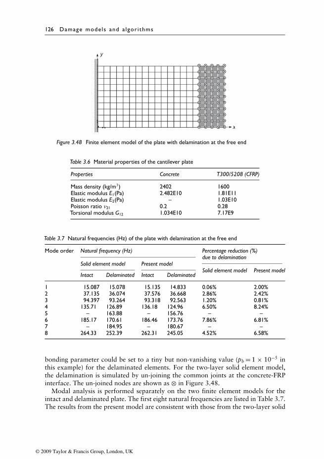
126 Damage mode ls and a lgor i thms
y
x
Figure 3.48 Finite element model of the plate with delamination at the free end
Table 3.6 Material properties of the cantilever plate
Properties Concrete T300/5208 (CFRP)
Mass density (kg/m3) 2402 1600Elastic modulus E1(Pa) 2.482E10 1.81E11Elastic modulus E2(Pa) – 1.03E10Poisson ratio ν21 0.2 0.28Torsional modulus G12 1.034E10 7.17E9
Table 3.7 Natural frequencies (Hz) of the plate with delamination at the free end
Mode order Natural frequency (Hz) Percentage reduction (%)due to delamination
Solid element model Present modelSolid element model Present model
Intact Delaminated Intact Delaminated
1 15.087 15.078 15.135 14.833 0.06% 2.00%2 37.135 36.074 37.576 36.668 2.86% 2.42%3 94.397 93.264 93.318 92.563 1.20% 0.81%4 135.71 126.89 136.18 124.96 6.50% 8.24%5 – 163.88 – 156.76 – –6 185.17 170.61 186.46 173.76 7.86% 6.81%7 – 184.95 – 180.67 – –8 264.33 252.39 262.31 245.05 4.52% 6.58%
bonding parameter could be set to a tiny but non-vanishing value (pb = 1 × 10⁻⁵ inthis example) for the delaminated elements. For the two-layer solid element model,the delamination is simulated by un-joining the common joints at the concrete-FRPinterface. The un-joined nodes are shown as ⊗ in Figure 3.48.
Modal analysis is performed separately on the two finite element models for theintact and delaminated plate. The first eight natural frequencies are listed in Table 3.7.The results from the present model are consistent with those from the two-layer solid
© 2009 Taylor & Francis Group, London, UK
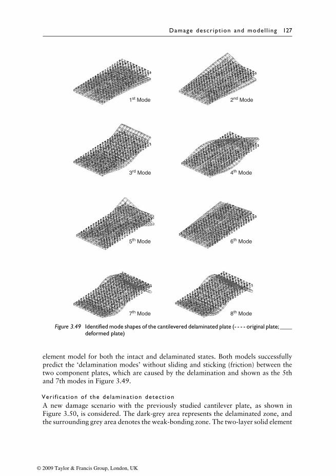
Damage descr ipt ion and mode l l ing 127
1st Mode 2nd Mode
3rd Mode 4th Mode
5th Mode 6th Mode
7th Mode 8th Mode
Figure 3.49 Identified mode shapes of the cantilevered delaminated plate (- - - - original plate;____deformed plate)
element model for both the intact and delaminated states. Both models successfullypredict the ‘delamination modes’ without sliding and sticking (friction) between thetwo component plates, which are caused by the delamination and shown as the 5thand 7th modes in Figure 3.49.
Ver i f i ca t ion of the de laminat ion detect ionA new damage scenario with the previously studied cantilever plate, as shown inFigure 3.50, is considered. The dark-grey area represents the delaminated zone, andthe surrounding grey area denotes the weak-bonding zone. The two-layer solid element
© 2009 Taylor & Francis Group, London, UK
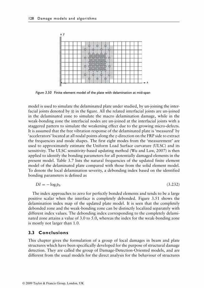
128 Damage mode ls and a lgor i thms
y
x
Figure 3.50 Finite element model of the plate with delamination at mid-span
model is used to simulate the delaminated plate under studied, by un-joining the inter-facial joints denoted by ⊗ in the figure. All the related interfacial joints are un-joinedin the delaminated zone to simulate the macro delamination damage, while in theweak-bonding zone the interfacial nodes are un-joined at the interfacial joints with astaggered pattern to simulate the weakening effect due to the growing micro-defects.It is assumed that the free vibration response of the delaminated plate is ‘measured’ by‘accelerators’ located at all nodal points along the z-direction on the FRP side to extractthe frequencies and mode shapes. The first eight modes from the ‘measurement’ areused to approximately estimate the Uniform Load Surface curvature (ULSC) and itssensitivity. The ULSC sensitivity-based updating method (Wu and Law, 2007) is thenapplied to identify the bonding parameters for all potentially damaged elements in thepresent model. Table 3.7 lists the natural frequencies of the updated finite elementmodel of the delaminated plate compared with those from the solid element model.To denote the local delamination severity, a debonding index based on the identifiedbonding parameters is defined as
DI = − log pb (3.232)
The index approaches to zero for perfectly bonded elements and tends to be a largepositive scalar when the interface is completely debonded. Figure 3.51 shows thedelamination index map of the updated plate model. It is seen that the completelydebonded zone and the weak-bonding zone can be distinctly localized separately withdifferent index values. The debonding index corresponding to the completely delami-nated zone attains a value of 3.0 to 5.0, whereas the index for the weak-bonding zoneis mostly not larger than 1.0.
3.3 Conclusions
This chapter gives the formulation of a group of local damages in beam and platestructures which have been specifically developed for the purpose of structural damagedetection. They are called the group of Damage-Detection-Oriented models, and aredifferent from the usual models for the direct analysis for the behaviour of structures
© 2009 Taylor & Francis Group, London, UK
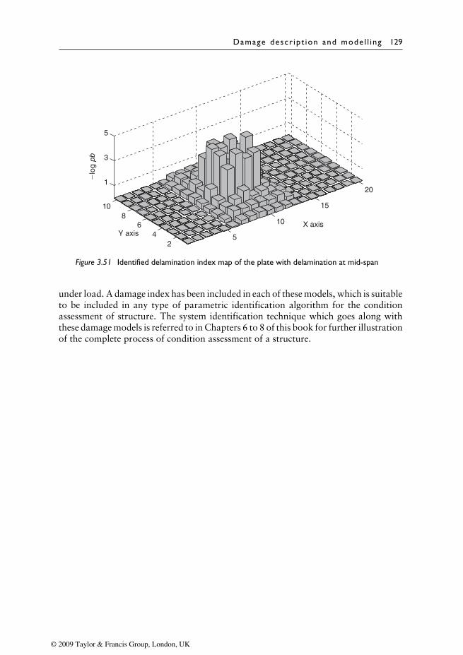
Damage descr ipt ion and mode l l ing 129
5
10
15
20
24
68
10
1
3
5
X axisY axis
�lo
g pb
Figure 3.51 Identified delamination index map of the plate with delamination at mid-span
under load. A damage index has been included in each of these models, which is suitableto be included in any type of parametric identification algorithm for the conditionassessment of structure. The system identification technique which goes along withthese damage models is referred to in Chapters 6 to 8 of this book for further illustrationof the complete process of condition assessment of a structure.
© 2009 Taylor & Francis Group, London, UK
Chapter 4
Model reduction
4.1 Introduction
It is computationally expensive and sometimes difficult to determine the natural fre-quencies and mode shapes for a structure with a large number of elements using thefull finite element model. For the inverse problems in structural analysis, the dynamicresponses of a structure required for the system identification are usually measured,and it is difficult and impractical to obtain the responses at all the degrees-of-freedom(DOFs) of the structure. It is desirable to reduce the size of the system matrices to havea more manageable and economic solution for both the direct and inverse problemsfrom only the responses of the measured DOFs. Such a reduction is usually referred toas the ‘model condensation method’. Another technique, called the ‘model expansionmethod’, to solve the problem of limited measured DOFs of a structure and the largenumber of DOFs of a structure is also presented in this chapter.
4.2 Static condensation
The oldest and perhaps the most popular model condensation method is theGuyan/Irons method (Guyan, 1965; Irons, 1965), which is applicable to both the staticand dynamic problems. Since the dynamic effect is ignored in the condensation, thismethod is usually referred to as the ‘static condensation’.
Considering a system with a static force, Fm, applied at some selected DOFs, itsstiffness matrix and response vector can be partitioned as[
Kmm Kms
Ksm Kss
]{xm
xs
}={
Fm
0
}(4.1)
where m and s denote the master (selected) DOFs and slave (truncated) DOFs, respec-tively. Combining the upper and lower parts of Equation (4.1), the relationship betweenthe selected response xm and the truncated response xs is
xs = −K−1ss Ksmxm (4.2)
The response vector can be described using the selected response xm only as
© 2009 Taylor & Francis Group, London, UK
132 Damage mode ls and a lgor i thms
x ={
xm
xs
}=[
I−K−1
ss Ksm
]xm = Tsxm (4.3)
where Ts =[
I−K−1
ss Ksm
]is the static transformation matrix between the full state
vector x and the master coordinates xm. The condensed system matrix, MRs, KRs, canthen be expressed as
MRs = TTs MTs, KRs = TT
s KTs (4.4)
where M and K are the system matrices before reduction. The eigen-solution for thecondensed system can be denoted as
(KRs − ω2MRs)φm = 0 (4.5)
where ω2 and φm are the eigenvalues and eigenvectors of the condensed system,respectively.
It should be noted that the incorrect selection of the master DOFs may result in asingularity in the eigenvalue problem. Different selection schemes (Shan and Raymund,1982; Matta, 1987) have been developed to improve the accuracy of the eigenvalueproblem. These schemes are also applicable to other methods referred to in this chapter.
It is noted that any frequency-response function generated from the reduced matricesin Equation (4.4) is exact only at zero frequency. In a dynamic system, the inertia effectincreases with increasing frequency, and the static condensation method may lead toa significant error. Therefore, dynamic condensation methods have subsequently beendeveloped to avoid this deficiency.
4.3 Dynamic condensation
A reduction method including the dynamic effects, known as the ‘dynamic conden-sation method’, is discussed in this section (Kuhar and Stahle, 1974; Miller, 1980).Inertia terms that were omitted in Equation (4.1) are included to give[
Mmm Mms
Msm Mss
]{xm
xs
}+[Kmm Kms
Ksm Kss
]{xm
xs
}= 0 (4.6)
Thus, the eigenvalue problem becomes(−ω2
[Mmm Mms
Msm Mss
]+[Kmm Kms
Ksm Kss
]){xm
xs
}= 0 (4.7)
The slave vector of responses, xs, may again be solved in terms of xm as
xs = −[Kss − ω2Mss]−1[Ksm − ω2Msm]xm
= Tdxm (4.8)
© 2009 Taylor & Francis Group, London, UK
Model reduct ion 133
where Td = − [Kss − ω2Mss]−1[Ksm − ω2Msm] is the dynamic transformation matrixbetween the full state vector and the master coordinates. The eigenvalue problem ofthe reduced system becomes
(−ω2(Mmm − MmsTd) + (Kmm − KmsTd))xm = 0 (4.9)
Note that the eigenvalue, ω, in Td is unknown. It can be found by using an iterativeprocess to find the transformation matrix with the set of initial eigenvalues equal tozero. A new eigenvalue vector based on the updated transformation matrix is thencalculated from Equation (4.9) and the process is repeated until the eigenvalue nolonger changes.
After obtaining the dynamic transformation matrix, the reduced system matrix canbe calculated as
MRd = TTd MTd, KRd = TT
d KTd (4.10)
To avoid the matrix inversion of Td in Equation (4.8), the first term on the right-hand-side is expanded into a Taylor series (Gordis, 1992) with the higher order termslarger than ω2 neglected, so Td becomes
Td = −[Kss − ω2Mss]−1[Ksm − ω2Msm] = −K−1ss [I − ω2MssK−1
ss ]−1[Ksm − ω2Msm]
= −K−1ss [I + ω2MssK−1
ss ][Ksm − ω2Msm]
= −K−1ss [Ksm + ω2(MssK−1
ss Ksm − Msm)] (4.11)
Substituting Equations (4.8) and (4.11) into Equation (4.7) and neglecting the higherorder terms, gives
ω2(Mmm − MmsK−1ss Ksm − KmsK−1
ss MssK−1ss Ksm)xm = (Kmm − KmsK−1
ss Ksm)xm (4.12)
Thus, the eigenvalue can be determined directly from Equation (4.12) without arequirement of iteration. Actually, this eigenvalue is the same as the one calculatedfrom the reduced model using the Guyan/Irons method, which can be expressed as
ω2MRsφm = KRsφm (4.13)
where MRs and KRs are already shown in Equation (4.4). Using the relationship inEquation (4.13), the dynamic transformation matrix Td can be modified as
Tid = −K−1ss [Ksm + (MssK−1
ss Ksm − Msm)M−1R KR] (4.14)
where Tid is the transformation matrix referred to in Equation (4.10). This modelcondensation method is called the Improved Reduction System (IRS) method.
This IRS method was originally proposed by O’Callahan (1989) with a differ-ent formulation but giving the same transformation matrix. The following gives theformulation developed by O’Callahan for further comparison.
© 2009 Taylor & Francis Group, London, UK
134 Damage mode ls and a lgor i thms
Considering a vector of static force, F, acting on all the DOFs of a structure andwith the same partitioning as in the Guyan/Irons method, Equation (4.1) becomes[
Kmm Kms
Ksm Kss
]{xm
xs
}={
Fm
Fs
}(4.15)
where Fs is the applied force on the slave DOFs. The truncated set of equation becomes
Ksmxm + Kssxs = Fs (4.16)
Solving for xs in Equation (4.16), gives
xs = −K−1ss Ksmxm + K−1
ss Fs (4.17)
Thus, the full state vector, x, can be expressed as
x = Tsxm + xFd (4.18)
where Ts is demonstrated in Equation (4.3) and xFd is the displacement adjustmentfrom the truncated distributed force defined as
xFd ={
0K−1
ss Fs
}=[0 00 K−1
ss
]F = K−1
s F (4.19)
According to Equations (4.13) and (4.15), the full space modal vector, φ, can beexpressed by φm using the same static reduction, that is φ= Tsφm, and xFd can beobtain as
xFd = K−1s MTsφmω
2 = K−1ss MssTsM−1
R KRφm (4.20)
then
x = (Ts + K−1ss MssTsM−1
R KR)φm = TIRSφm (4.21)
where
TIRS = −K−1ss [Ksm + (MssK−1
ss Ksm − Msm)M−1R KR] (4.22)
Note that TIRS in Equation (4.22) is identical to Tid in Equation (4.14).The mass and stiffness matrices obtained from using the transformation matrix in
Equation (4.22) or Equation (4.14) exhibit improved system characteristics comparedto those obtained from static condensation with the inertia effects included. The massand stiffness matrices for the improved reduced system are thus
MRI = TTIRSMTIRS, KRI = TT
IRSKTIRS (4.23)
The quality of the IRS results is relatively insensitive to the number and location of theselected DOFs compared with the methods mentioned in previous sections.
Other dynamic condensation methods and iterative methods involving eigenvalueanalysis have also been developed. An accurate method of dynamic condensation with
© 2009 Taylor & Francis Group, London, UK
Model reduct ion 135
a simplified computation for sub-structures was developed by Leung (1978; 1979). Animproved dynamic condensation approach was developed by Suarez and Singh (1992)for structural eigenvalue analysis, which can use the kept and reduced DOFs separatelyor together to calculate the total eigen-solution of the system.
4.4 Iterative condensation
Improvements have been proposed by other researchers which modify the method intoan iterative process. Such a method is called the Iterative IRS method (IIRS). Thereare two types of IIRS method. The first one was proposed by Blair (1991). Since thetransformation matrix for the IRS method makes use of the reduced mass and stiffnessmatrices obtained from the Guyan/Irons method, an improved transformation matrixcan be constructed using the newly approximated matrices described in Equation (4.23)via iterations with Equation (4.22) as
TIRS,i+1 = −K−1ss [Ksm + (MssTs − Msm)M−1
RI,iKRI,i] (4.24)
where i is the number of iterations. Equation (4.23) becomes
MRI,i+1 = TTIRS,i+1MTIRS,i+1, KRI,i+1 = TT
IRS,i+1KTIRS,i+1 (4.25)
The second type of IIRS method (Friswell et al., 1995) further incorporates the trans-formation matrix from the last iteration in the computation by modifying Equation(4.24) as
TIRS,i+1 = −K−1ss [Ksm + (MssTIRS,i − Msm)M−1
RI,iKRI,i] (4.26)
The two types of iterative method are quite similar and both of them show goodaccuracy for model reduction. Another iterative scheme for dynamic condensationwas also introduced by Qu and Fu (2000) and the full proof of its convergence wasgiven. Two criteria for the computation convergence were introduced with improvedcomputational efficiency.
4.5 Moving force identification using the improvedreduced system
4.5.1 Theory of moving force identif ication
The equation of motion for the vehicle-bridge system can be written as (Law et al.,2004a)
MbR + CbR + KbR = HcPint (4.27)
where Mb, Cb and Kb are the mass, damping and stiffness matrices of the bridge,respectively; R, R and R are the nodal acceleration, velocity and displacement vectorsof the bridge, respectively; and HcPint is the equivalent nodal load vector of the bridge-vehicle interaction force with
Hc ={
0 · · · 0 · · · H1 · · · 00 · · · H2 · · · 0 · · · 0
}T
© 2009 Taylor & Francis Group, London, UK
136 Damage mode ls and a lgor i thms
Hc is an NN × Np matrix with zero entries, except at the DOFs corresponding tothe nodal displacements of the beam elements on which the load is acting; and NNis the number of DOFs of the bridge after considering the boundary condition.
From Equation (4.27), the strain at a point x and at time t can be written as
ε(x, t) = −z∂2H(x) R(t)∂x2
(4.28)
where z represents the distance from the neutral axis of the beam to the bottom surface.The Improved Reduced System reduction scheme (O’Callahan, 1989) is adopted to
condense the unmeasured DOFs to the measured DOFs of the bridge deck. All the mea-sured DOFs are designated as the master DOFs and denoted by Rm(t). The remainingstructural DOFs are called the slave DOFs, and are denoted by Rs(t). The responsevector of the bridge is then partitioned as
R(t) ={
Rm(t)Rs(t)
}(4.29)
Accordingly, the bridge mass, damping, stiffness and shape function matrices are alsopartitioned as
Mb =[Mmm Mms
Msm Mss
], Cb =
[Cmm Cms
Csm Css
], Kb =
[Kmm Kms
Ksm Kss
],
H =[Hmm
Hss
]T
, Hc =[Hcmm
Hcss
](4.30)
The total response matrix of the system, R(t), can then be represented by a parti-tioned matrix related to the master set of DOFs Rm(t) multiplied by the transformationmatrix as
R(t) = W Rm(t), (4.31)
where W = Ws + Wi, Ws =[
I−K−1
ss Ksm
]and Wi =
[I
K−1ss (Msm − MssK−1
ss Ksm)(WTs MbWs)−1(WT
s KbWs)
].
where I is the identity matrix. Substituting Equations (4.30) and (4.31) into Equation(4.27) and pre-multiplying WT on both sides, gives
U = Hcr Pint (4.32)
and U = MrRm + CrRm + KrRm
where Mr = WTMbW , Cr = WTCbW , Kr = WTKbW , and Hcr = WTHc.
Substituting Equation (4.31) and H =[Hmm
Hss
]T
into Equation (4.28), matrices
Rm, Rm and Rm can be obtained by the generalized orthogonal function method.
© 2009 Taylor & Francis Group, London, UK
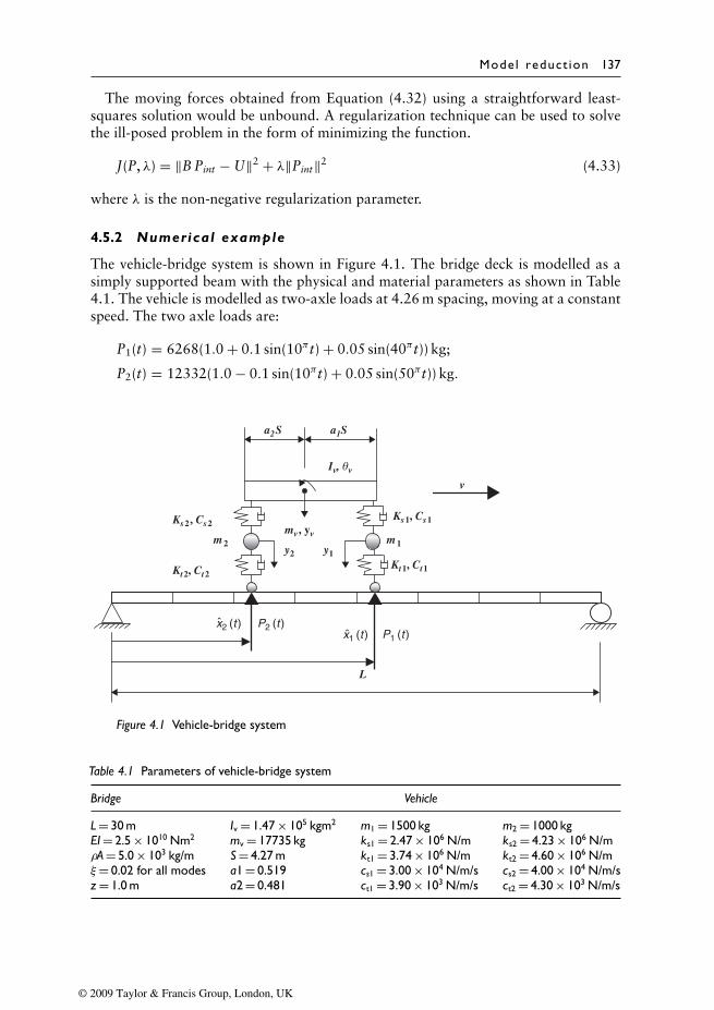
Model reduct ion 137
The moving forces obtained from Equation (4.32) using a straightforward least-squares solution would be unbound. A regularization technique can be used to solvethe ill-posed problem in the form of minimizing the function.
J(P, λ) = ‖B Pint − U‖2 + λ‖Pint‖2 (4.33)
where λ is the non-negative regularization parameter.
4.5.2 Numerical example
The vehicle-bridge system is shown in Figure 4.1. The bridge deck is modelled as asimply supported beam with the physical and material parameters as shown in Table4.1. The vehicle is modelled as two-axle loads at 4.26 m spacing, moving at a constantspeed. The two axle loads are:
P1(t) = 6268(1.0 + 0.1 sin(10πt) + 0.05 sin(40πt)) kg;
P2(t) = 12332(1.0 − 0.1 sin(10πt) + 0.05 sin(50πt)) kg.
Ks2, Cs2 Ks1, Cs1
Kt2, Ct2Kt1, Ct1
m2 m1
a2S a1S
mv, yv
Iv, θv
y1y2
L
x1 (t )x2 (t )
P1 (t )P2 (t )
v
Figure 4.1 Vehicle-bridge system
Table 4.1 Parameters of vehicle-bridge system
Bridge Vehicle
L = 30 m Iv = 1.47 × 10⁵ kgm2 m1 = 1500 kg m2 = 1000 kgEI = 2.5 × 10¹⁰ Nm2 mv = 17735 kg ks1 = 2.47 × 10⁶ N/m ks2 = 4.23 × 10⁶ N/mρA = 5.0 × 10³ kg/m S = 4.27 m kt1 = 3.74 × 10⁶ N/m kt2 = 4.60 × 10⁶ N/mξ= 0.02 for all modes a1 = 0.519 cs1 = 3.00 × 10⁴ N/m/s cs2 = 4.00 × 10⁴ N/m/sz = 1.0 m a2 = 0.481 ct1 = 3.90 × 10³ N/m/s ct2 = 4.30 × 10³ N/m/s
© 2009 Taylor & Francis Group, London, UK
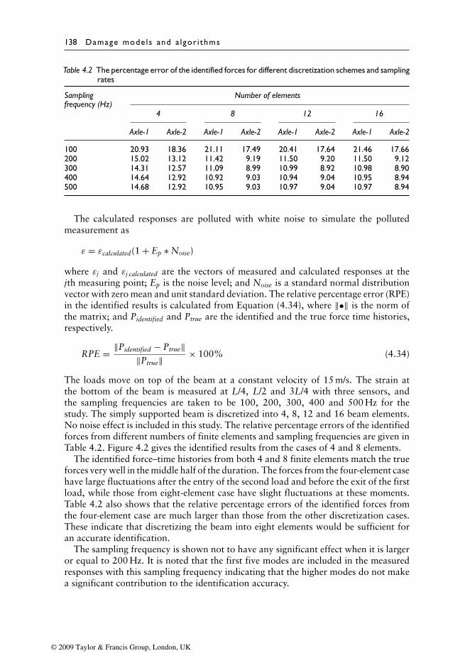
138 Damage mode ls and a lgor i thms
Table 4.2 The percentage error of the identified forces for different discretization schemes and samplingrates
Sampling Number of elementsfrequency (Hz)
4 8 12 16
Axle-1 Axle-2 Axle-1 Axle-2 Axle-1 Axle-2 Axle-1 Axle-2
100 20.93 18.36 21.11 17.49 20.41 17.64 21.46 17.66200 15.02 13.12 11.42 9.19 11.50 9.20 11.50 9.12300 14.31 12.57 11.09 8.99 10.99 8.92 10.98 8.90400 14.64 12.92 10.92 9.03 10.94 9.04 10.95 8.94500 14.68 12.92 10.95 9.03 10.97 9.04 10.97 8.94
The calculated responses are polluted with white noise to simulate the pollutedmeasurement as
ε = εcalculated(1 + Ep ∗ Noise)
where εj and εj calculated are the vectors of measured and calculated responses at thejth measuring point; Ep is the noise level; and Noise is a standard normal distributionvector with zero mean and unit standard deviation. The relative percentage error (RPE)in the identified results is calculated from Equation (4.34), where ‖•‖ is the norm ofthe matrix; and Pidentified and Ptrue are the identified and the true force time histories,respectively.
RPE = ‖Pidentified − Ptrue‖‖Ptrue‖ × 100% (4.34)
The loads move on top of the beam at a constant velocity of 15 m/s. The strain atthe bottom of the beam is measured at L/4, L/2 and 3L/4 with three sensors, andthe sampling frequencies are taken to be 100, 200, 300, 400 and 500 Hz for thestudy. The simply supported beam is discretized into 4, 8, 12 and 16 beam elements.No noise effect is included in this study. The relative percentage errors of the identifiedforces from different numbers of finite elements and sampling frequencies are given inTable 4.2. Figure 4.2 gives the identified results from the cases of 4 and 8 elements.
The identified force–time histories from both 4 and 8 finite elements match the trueforces very well in the middle half of the duration. The forces from the four-element casehave large fluctuations after the entry of the second load and before the exit of the firstload, while those from eight-element case have slight fluctuations at these moments.Table 4.2 also shows that the relative percentage errors of the identified forces fromthe four-element case are much larger than those from the other discretization cases.These indicate that discretizing the beam into eight elements would be sufficient foran accurate identification.
The sampling frequency is shown not to have any significant effect when it is largeror equal to 200 Hz. It is noted that the first five modes are included in the measuredresponses with this sampling frequency indicating that the higher modes do not makea significant contribution to the identification accuracy.
© 2009 Taylor & Francis Group, London, UK
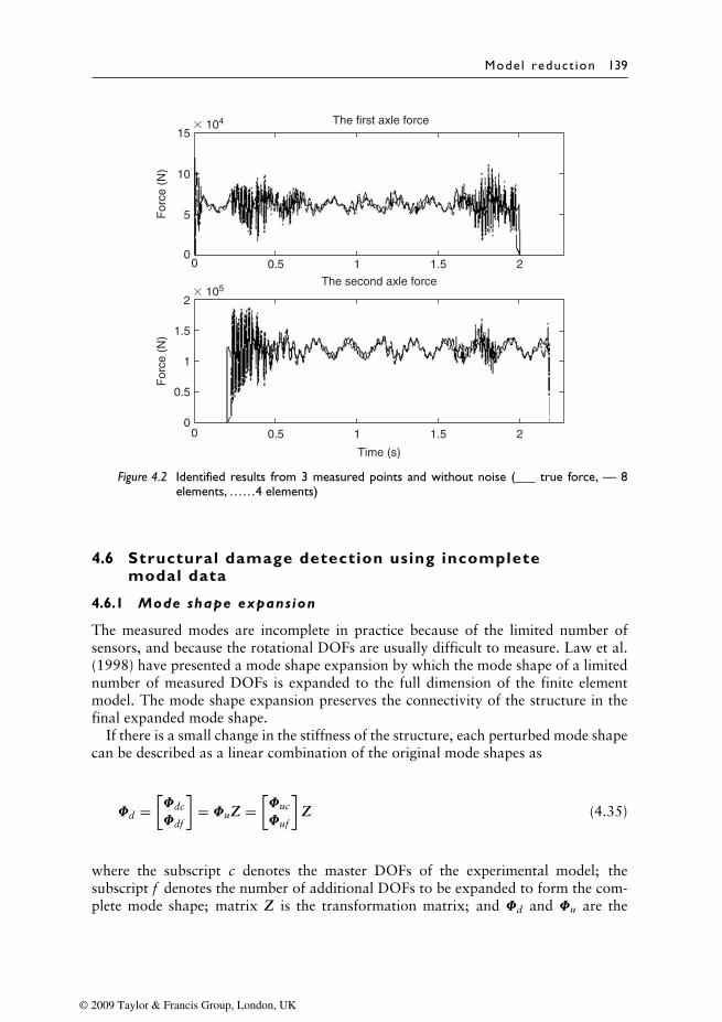
Model reduct ion 139
0.500
5
10
15
1 1.5 2
The first axle force
For
ce (
N)
� 104
The second axle force
0.500
0.5
1.5
1
2
1
Time (s)
1.5 2
For
ce (
N)
� 105
Figure 4.2 Identified results from 3 measured points and without noise (___ true force, — 8elements, ……4 elements)
4.6 Structural damage detection using incompletemodal data
4.6.1 Mode shape expansion
The measured modes are incomplete in practice because of the limited number ofsensors, and because the rotational DOFs are usually difficult to measure. Law et al.(1998) have presented a mode shape expansion by which the mode shape of a limitednumber of measured DOFs is expanded to the full dimension of the finite elementmodel. The mode shape expansion preserves the connectivity of the structure in thefinal expanded mode shape.
If there is a small change in the stiffness of the structure, each perturbed mode shapecan be described as a linear combination of the original mode shapes as
Φd =[Φdc
Φdf
]= ΦuZ =
[Φuc
Φuf
]Z (4.35)
where the subscript c denotes the master DOFs of the experimental model; thesubscript f denotes the number of additional DOFs to be expanded to form the com-plete mode shape; matrix Z is the transformation matrix; and Φd and Φu are the
© 2009 Taylor & Francis Group, London, UK
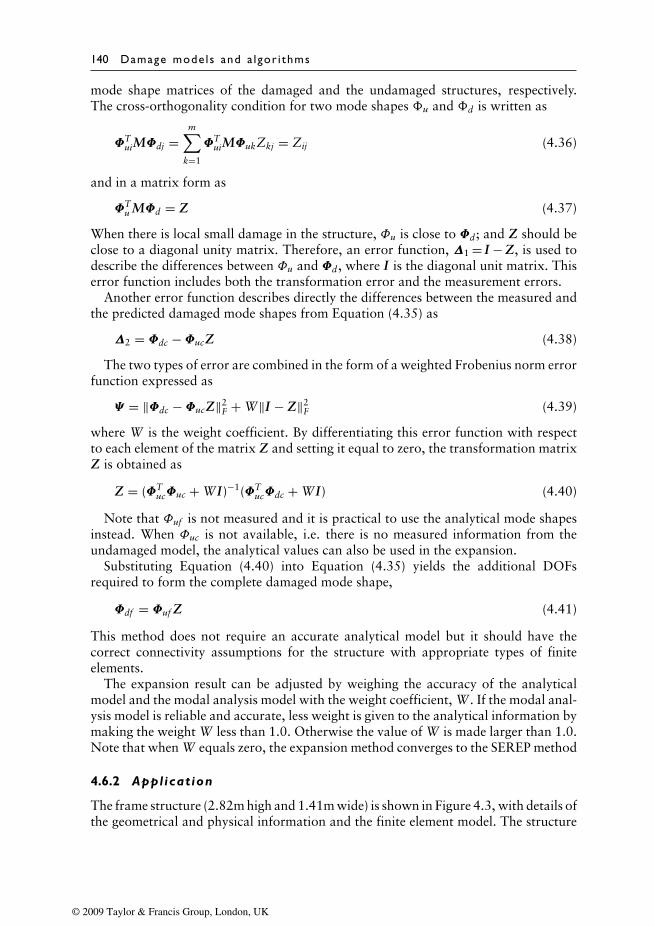
140 Damage mode ls and a lgor i thms
mode shape matrices of the damaged and the undamaged structures, respectively.The cross-orthogonality condition for two mode shapes �u and �d is written as
ΦTuiMΦdj =
m∑k=1
ΦTuiMΦukZkj = Zij (4.36)
and in a matrix form as
ΦTu MΦd = Z (4.37)
When there is local small damage in the structure, Φu is close to Φd; and Z should beclose to a diagonal unity matrix. Therefore, an error function, ∆1 = I − Z, is used todescribe the differences between Φu and Φd, where I is the diagonal unit matrix. Thiserror function includes both the transformation error and the measurement errors.
Another error function describes directly the differences between the measured andthe predicted damaged mode shapes from Equation (4.35) as
∆2 = Φdc − ΦucZ (4.38)
The two types of error are combined in the form of a weighted Frobenius norm errorfunction expressed as
Ψ = ‖Φdc − ΦucZ‖2F + W‖I − Z‖2
F (4.39)
where W is the weight coefficient. By differentiating this error function with respectto each element of the matrix Z and setting it equal to zero, the transformation matrixZ is obtained as
Z = (ΦTucΦuc + WI)−1(ΦT
ucΦdc + WI) (4.40)
Note that Φuf is not measured and it is practical to use the analytical mode shapesinstead. When Φuc is not available, i.e. there is no measured information from theundamaged model, the analytical values can also be used in the expansion.
Substituting Equation (4.40) into Equation (4.35) yields the additional DOFsrequired to form the complete damaged mode shape,
Φdf = Φuf Z (4.41)
This method does not require an accurate analytical model but it should have thecorrect connectivity assumptions for the structure with appropriate types of finiteelements.
The expansion result can be adjusted by weighing the accuracy of the analyticalmodel and the modal analysis model with the weight coefficient, W . If the modal anal-ysis model is reliable and accurate, less weight is given to the analytical information bymaking the weight W less than 1.0. Otherwise the value of W is made larger than 1.0.Note that when W equals zero, the expansion method converges to the SEREP method
4.6.2 Application
The frame structure (2.82m high and 1.41m wide) is shown in Figure 4.3, with details ofthe geometrical and physical information and the finite element model. The structure
© 2009 Taylor & Francis Group, London, UK
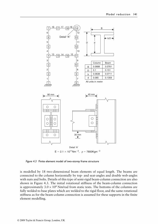
Model reduct ion 141
Detail “A”
7
6
5
413 14 15
15 16
171716
1818
14
12
1
2
3
4
5
6
11
10
12
11 D d
b/213
3
2
1 8
9
7
8
10
9
All units in metre
B
D
b
d
Column
0.0688
0.1
0.0638
0.085
Beam
0.0761
0.151
0.0711
0.1359
80 mm
30 mm
Detail ‘A’
40 mm
B
E � 2.1 � 1011Nm�2, ρ � 7800Kgm�3
Figure 4.3 Finite element model of two-storey frame structure
is modelled by 18 two-dimensional beam elements of equal length. The beams areconnected to the column horizontally by top- and seat-angles and double web-angleswith nuts and bolts. Details of this type of semi-rigid beam-column connection are alsoshown in Figure 4.3. The initial rotational stiffness of the beam-column connectionis approximately 3.0 × 10⁶ Nm/rad from static tests. The bottoms of the columns arefully welded to base plates which are welded to the rigid floor, and the same rotationalstiffness as for the beam-column connection is assumed for these supports in the finiteelement modelling.
© 2009 Taylor & Francis Group, London, UK
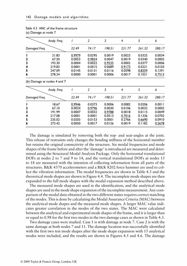
142 Damage mode ls and a lgor i thms
Table 4.3 MAC of the frame structure(a) Damage at node 7
————————————–
Analy. Freq. 1 2 3 4 5 6
Damaged Freq. 22.49 74.17 198.51 221.77 261.32 280.17
1 21.83 0.9979 0.0295 0.0019 0.0023 0.0325 0.00342 67.50 0.0053 0.9834 0.0047 0.0019 0.0340 0.00023 193.30 0.0004 0.0022 0.9535 0.0002 0.0377 0.00064 219.83 0.0001 0.0015 0.0689 0.9173 0.0221 0.01035 247.09 0.0145 0.0131 0.0116 0.0598 0.8359 0.12916 278.24 0.0000 0.0001 0.0006 0.0017 0.1021 0.7513
(b) Damage at nodes 4 and 7
————————————–
Analy. Freq. 1 2 3 4 5 6
Damaged Freq. 22.49 74.17 198.51 221.77 261.32 280.17
1 18.67 0.9946 0.0373 0.0006 0.0082 0.0206 0.00112 67.10 0.0024 0.9796 0.0030 0.0106 0.0032 0.00023 191.99 0.0007 0.0032 0.9788 0.0018 0.0115 0.00494 217.08 0.0001 0.0001 0.0513 0.7016 0.1336 0.07025 235.02 0.0203 0.0153 0.0001 0.2766 0.6690 0.09106 273.42 0.0050 0.0017 0.0126 0.0019 0.1182 0.5678
The damage is simulated by removing both the top- and seat-angles at the joint.This release of restraints only changes the bending stiffness of the horizontal memberbut retains the original connectivity of the structure. Six modal frequencies and modeshapes of the frame before and after the ‘damage’ is introduced are measured and deter-mined using the Structural Modal Analysis Package. Only the horizontal translationalDOFs at nodes 2 to 7 and 9 to 14, and the vertical translational DOFs at nodes 15to 18 are measured with the intention of collecting information from all parts of thestructures. B&K 4370 accelerometers and a B&K 8202 force hammer are used to col-lect the vibration information. The modal frequencies are shown in Table 4.3 and thetheoretical mode shapes are shown in Figure 4.4. The incomplete mode shapes are thenexpanded to the full mode shapes with the modal expansion method described above.
The measured mode shapes are used in the identification, and the analytical modeshapes are used in the mode shape expansion of the incomplete measurement. Any com-parison of the modal data obtained in the two different states requires correct matchingof the modes. This is done by calculating the Modal Assurance Criteria (MAC) betweenthe analytical mode shapes and the measured mode shapes. A larger MAC value indi-cates greater correlation in the modes of the two states. The MAC were calculatedbetween the analytical and experimental mode shapes of the frame, and it is larger thanor equal to 0.98 for the first two modes in the two damage cases as shown in Table 4.3.
Two damage cases were studied. Case 1 is with damage at node 7. Case 2 is with thesame damage at both nodes 7 and 11. The damage location was successfully identifiedwith the first two test mode shapes after the mode shape expansion with 15 analyticalmodes were included, and the results are shown in Figures 4.5 and 4.6. The damage
© 2009 Taylor & Francis Group, London, UK
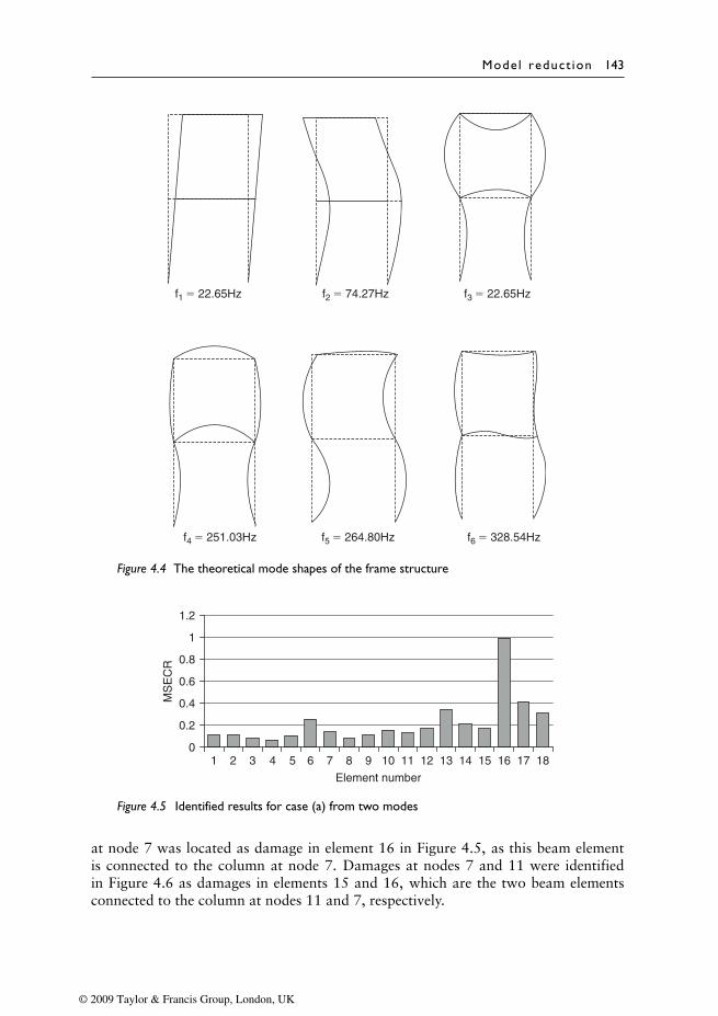
Model reduct ion 143
f1 � 22.65Hz f2 � 74.27Hz f3 � 22.65Hz
f6 � 328.54Hzf5 � 264.80Hzf4 � 251.03Hz
Figure 4.4 The theoretical mode shapes of the frame structure
0
0.2
0.4
0.6
0.8
1
1.2
1 2 3 4 5 6 7 8 9 10 11 12 13 14 15 16 17 18
MS
EC
R
Element number
Figure 4.5 Identified results for case (a) from two modes
at node 7 was located as damage in element 16 in Figure 4.5, as this beam elementis connected to the column at node 7. Damages at nodes 7 and 11 were identifiedin Figure 4.6 as damages in elements 15 and 16, which are the two beam elementsconnected to the column at nodes 11 and 7, respectively.
© 2009 Taylor & Francis Group, London, UK
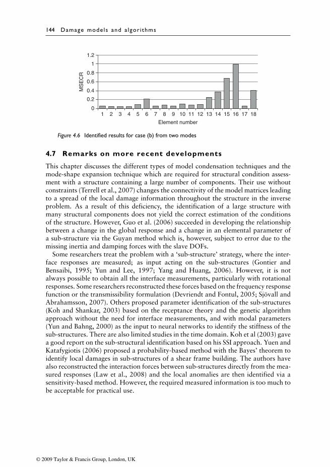
144 Damage mode ls and a lgor i thms
0
0.2
0.4
0.6
0.8
1
1.2
1 2 3 4 5 6 7 8 9 10 11 12 13 14 15 16 17 18
MS
EC
R
Element number
Figure 4.6 Identified results for case (b) from two modes
4.7 Remarks on more recent developments
This chapter discusses the different types of model condensation techniques and themode-shape expansion technique which are required for structural condition assess-ment with a structure containing a large number of components. Their use withoutconstraints (Terrell et al., 2007) changes the connectivity of the model matrices leadingto a spread of the local damage information throughout the structure in the inverseproblem. As a result of this deficiency, the identification of a large structure withmany structural components does not yield the correct estimation of the conditionsof the structure. However, Guo et al. (2006) succeeded in developing the relationshipbetween a change in the global response and a change in an elemental parameter ofa sub-structure via the Guyan method which is, however, subject to error due to themissing inertia and damping forces with the slave DOFs.
Some researchers treat the problem with a ‘sub-structure’ strategy, where the inter-face responses are measured; as input acting on the sub-structures (Gontier andBensaibi, 1995; Yun and Lee, 1997; Yang and Huang, 2006). However, it is notalways possible to obtain all the interface measurements, particularly with rotationalresponses. Some researchers reconstructed these forces based on the frequency responsefunction or the transmissibility formulation (Devriendt and Fontul, 2005; Sjövall andAbrahamsson, 2007). Others proposed parameter identification of the sub-structures(Koh and Shankar, 2003) based on the receptance theory and the genetic algorithmapproach without the need for interface measurements, and with modal parameters(Yun and Bahng, 2000) as the input to neural networks to identify the stiffness of thesub-structures. There are also limited studies in the time domain. Koh et al (2003) gavea good report on the sub-structural identification based on his SSI approach. Yuen andKatafygiotis (2006) proposed a probability-based method with the Bayes’ theorem toidentify local damages in sub-structures of a shear frame building. The authors havealso reconstructed the interaction forces between sub-structures directly from the mea-sured responses (Law et al., 2008) and the local anomalies are then identified via asensitivity-based method. However, the required measured information is too much tobe acceptable for practical use.
© 2009 Taylor & Francis Group, London, UK
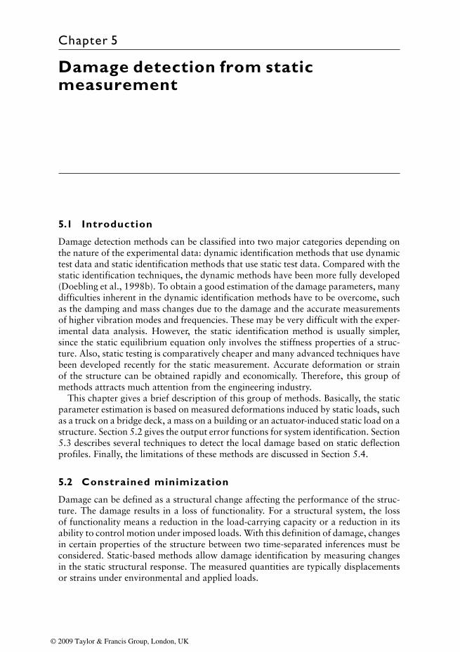
Chapter 5
Damage detection from staticmeasurement
5.1 Introduction
Damage detection methods can be classified into two major categories depending onthe nature of the experimental data: dynamic identification methods that use dynamictest data and static identification methods that use static test data. Compared with thestatic identification techniques, the dynamic methods have been more fully developed(Doebling et al., 1998b). To obtain a good estimation of the damage parameters, manydifficulties inherent in the dynamic identification methods have to be overcome, suchas the damping and mass changes due to the damage and the accurate measurementsof higher vibration modes and frequencies. These may be very difficult with the exper-imental data analysis. However, the static identification method is usually simpler,since the static equilibrium equation only involves the stiffness properties of a struc-ture. Also, static testing is comparatively cheaper and many advanced techniques havebeen developed recently for the static measurement. Accurate deformation or strainof the structure can be obtained rapidly and economically. Therefore, this group ofmethods attracts much attention from the engineering industry.
This chapter gives a brief description of this group of methods. Basically, the staticparameter estimation is based on measured deformations induced by static loads, suchas a truck on a bridge deck, a mass on a building or an actuator-induced static load on astructure. Section 5.2 gives the output error functions for system identification. Section5.3 describes several techniques to detect the local damage based on static deflectionprofiles. Finally, the limitations of these methods are discussed in Section 5.4.
5.2 Constrained minimization
Damage can be defined as a structural change affecting the performance of the struc-ture. The damage results in a loss of functionality. For a structural system, the lossof functionality means a reduction in the load-carrying capacity or a reduction in itsability to control motion under imposed loads. With this definition of damage, changesin certain properties of the structure between two time-separated inferences must beconsidered. Static-based methods allow damage identification by measuring changesin the static structural response. The measured quantities are typically displacementsor strains under environmental and applied loads.
© 2009 Taylor & Francis Group, London, UK
146 Damage mode l and a lgor i thms
5.2.1 Output error function
The first method to describe the changes in the static response is the output errorfunction. This is the difference between the analytical and measured static responses.The parameters are identified by minimizing an objective function formulated by theoutput error function (Hjelmstad and Shin, 1997) defined as the difference between thecomputed and measured displacements. A recursive quadratic programming algorithmwas used to solve the constrained nonlinear optimization problem. Sanayei et al. (1997)presented the output error function based on the static displacements and strains.Both static displacement and strain measurements are used to estimate the elementstiffness parameters. The method is extended to identify the element properties of atruss structure using static strains from a series of concentrated forces (Liu and Chian,1997), and the effect of measurement errors on the identified results was studied usingthe perturbation technique. Shenton and Hu (2006) presented a static procedure basedon the idea that the dead load is redistributed when damage occurs in the structure. Thestatic strain measurements due to dead load only are used for the damage identification.
5.2.1.1 Disp lacement output error funct ion
Consider a discrete structural system with nd degrees-of-freedom (DOFs), having astiffness matrix, K, characterized by np constitutive parameters, p. Let the structurebe separately subject to nf static load cases. For a linear elastic structure, the force–displacement relationship based on the finite element model is
fi = Kui (5.1)
where fi is the vector of applied forces for the ith load case and ui is the correspondingdisplacement vector.
The output error function is defined as the difference between the analytical andmeasured displacements for the ith load case as follows
ei(p) = K−1fi − ui (5.2)
where K−1 is the inverse of the stiffness matrix.Since the displacements are taken only at a subset of DOFs, matrix ui may be par-
titioned into uai and ubi, which are the measured and unmeasured displacements,respectively. Giving[
fai
fbi
]=[
Kaa Kab
Kba Kbb
] [uai
ubi
](5.3)
Using the static condensation
fai = (Kaa − KabK−1bb Kba)uai + KabK−1
bb fbi (5.4)
With the applied forces and measured responses, the output error function can bedefined as
ei(p) = (Kaa − KabK−1bb Kba)−1(fm
ai − KabK−1bb fm
bi) − umai (5.5)
© 2009 Taylor & Francis Group, London, UK
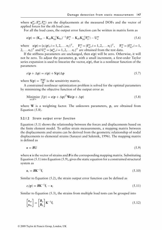
Damage detect ion from stat i c measurement 147
where umai , (fm
ai , fmbi) are the displacements at the measured DOFs and the vector of
applied forces for the ith load case.For all the load cases, the output error function can be written in matrix form as
e(p) = (Kaa − KabK−1bb Kba)−1(Fm
a − KabK−1bb Fm
b ) − Uma (5.6)
where e(p) = {ei(p), i = 1, 2, . . .nf }T , Fma = {fm
ai , i = 1, 2, . . .nf }T , Fmb = {fm
bi, i = 1,2, . . .nf }T and Um
a = {umai , i = 1, 2, . . .nf }T are obtained from the test data.
If the stiffness parameters are unchanged, then e(p) will be zero. Otherwise, it willnot be zero. To adjust the parameter, p, with a small increment, a first-order Taylorseries expansion is used to linearize the vector, e(p), that is a nonlinear function of theparameters
e(p +�p) = e(p) + S(p)�p (5.7)
where S(p) = ∂e(p)∂p is the sensitivity matrix.
A constrained nonlinear optimization problem is solved for the optimal parametersby minimizing the objective function of the output error as
Minimizeα∈Rnα
J(p) = e(p +�p)TWe(p +�p) (5.8)
where W is a weighting factor. The unknown parameters, p, are obtained fromEquation (5.8).
5.2.1.2 Stra in output error funct ion
Equation (5.1) shows the relationship between the forces and displacements based onthe finite element model. To utilize strain measurements, a mapping matrix betweenthe displacements and strains can be derived from the geometric relationship of nodaldisplacements to elemental strains (Sanayei and Saletnik, 1996). The mapping matrixis defined as
ε = BU (5.9)
where ε is the vector of strains and B is the corresponding mapping matrix. SubstitutingEquation (5.1) into Equation (5.9), gives the static equation for a constrained structuralsystem as
εi = BK−1fi (5.10)
Similar to Equation (5.2), the strain output error function can be defined as
ei(p) = BK−1fi − εi (5.11)
Similar to Equation (5.3), the strains from multiple load tests can be grouped into[εai
εbi
]=[
Ba
Bb
]K−1fi (5.12)
© 2009 Taylor & Francis Group, London, UK
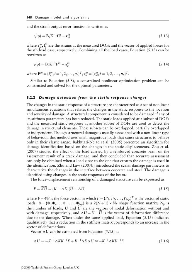
148 Damage mode l and a lgor i thms
and the strain output error function is written as
ei(p) = BaK−1fmi − εm
ai (5.13)
where εmai , fm
i are the strains at the measured DOFs and the vector of applied forces forthe ith load case, respectively. Combining all the load cases, Equation (5.13) can berewritten as
e(p) = BaK−1Fm − εma (5.14)
where Fm = {fmi , i = 1, 2, . . . , nf }T , εm
a = {εmai , i = 1, 2, . . . , nf }T .
Similar to Equation (5.8), a constrained nonlinear optimization problem can beconstructed and solved for the optimal parameters.
5.2.2 Damage detection from the static response changes
The changes in the static response of a structure are characterized as a set of nonlinearsimultaneous equations that relates the changes in the static response to the locationand severity of damage. A structural component is considered to be damaged if any ofits stiffness parameters has been reduced. The static loads applied at a subset of DOFsand the measured static response at another subset of DOFs are used to detect thedamage in structural elements. These subsets can be overlapped, partially overlappedor independent. Though structural damage is usually associated with a non-linear typeof behaviour, this method uses small magnitude loads that cause structures to behaveonly in their elastic range. Bakhtiari-Nejad et al. (2005) presented an algorithm fordamage identification based on the changes in the static displacements. Zhu et al.(2007) studied the effect of the load carried by a reinforced concrete beam on theassessment result of a crack damage, and they concluded that accurate assessmentcan only be obtained when a load close to the one that creates the damage is used inthe identification. Zhu and Law (2007b) introduced the scalar damage parameters tocharacterize the changes in the interface between concrete and steel. The damage isidentified using changes in the static responses of the beam.
The force–displacement relationship of a damaged structure can be expressed as
F = KU = (K −�K)(U −�U) (5.15)
where F =�P is the force vector, in which P = {P1, P2, . . . , PNp}T is the vector of staticloads; �= {�1�2 . . . �l . . . . . �Np} is a 2(N + 1) × Np shape function matrix; Np isthe number of loads; U and U are the vectors of nodal deformation without andwith damage, respectively; and �U = U − U is the vector of deformation differencedue to the damage. When under the same applied load, Equation (5.15) indicatesqualitatively that a reduction in the stiffness matrix corresponds to an increase in thevector of deformations.
Vector �U can be estimated from Equation (5.15) as
�U = −K−1�KK−1F + K−1�K�U ≈ −K−1�KK−1F (5.16)
© 2009 Taylor & Francis Group, London, UK
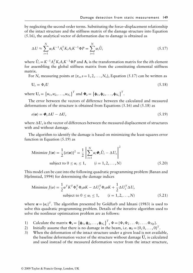
Damage detect ion from stat i c measurement 149
by neglecting the second-order terms. Substituting the force–displacement relationshipof the intact structure and the stiffness matrix of the damage structure into Equation(5.16), the analytical vector of deformation due to damage is obtained as
�U ≈N∑
i=1
αiK−1ATi KiAiK−1�P =
N∑i=1
αiUi (5.17)
where Ui = K−1ATi KiAiK−1�P and Ai is the transformation matrix for the ith element
for assembling the global stiffness matrix from the constituting elemental stiffnessmatrix.
For Ns measuring points at {xs, s = 1, 2, . . . , Ns}, Equation (5.17) can be written as
Us = �sU (5.18)
where Us = {u1, u2, . . . , uNs
}T and �s = {φ1, φ2, . . . , φNs
}T .
The error between the vectors of difference between the calculated and measureddeformations of the structure is obtained from Equations (5.16) and (5.18) as
e(α) = Φs�U −�U s (5.19)
where�U s is the vector of differences between the measured displacement of structureswith and without damage.
The algorithm to identify the damage is based on minimizing the least-squares errorfunction in Equation (5.19) as
Minimize J(α) = 12
‖e(α)‖2 = 12
∥∥∥∥∥N∑
i=1
αiΦsUi −�Us
∥∥∥∥∥2
subject to 0 ≤ αi ≤ 1, (i = 1, 2, . . . , N) (5.20)
This model can be cast into the following quadratic programming problem (Banan andHjelmstad, 1994) for determining the damage indices
Minimize J(α) = 12αTKT�T
s �sαK −�UTs �sαK + 1
2�UT
s �Us
subject to 0 ≤ αi ≤ 1, (i = 1, 2, . . . , N) (5.21)
where α = {αi}T . The algorithm presented by Goldfarb and Idnani (1983) is used tosolve this quadratic programming problem. Details of the iterative algorithm used tosolve the nonlinear optimization problem are as follows:
1) Calculate the matrix �s = {φ1, φ2, . . . , φNs
}T , �= {�1�2 . . . �l . . . ..�Np}.2) Initially assume that there is no damage in the beam, i.e. α0 = {0, 0, . . . , 0}T .3) When the deformation of the intact structure under a given load is not available,
the baseline deformation vector of the structure without damage Us is calculatedand used instead of the measured deformation vector from the intact structure,
© 2009 Taylor & Francis Group, London, UK
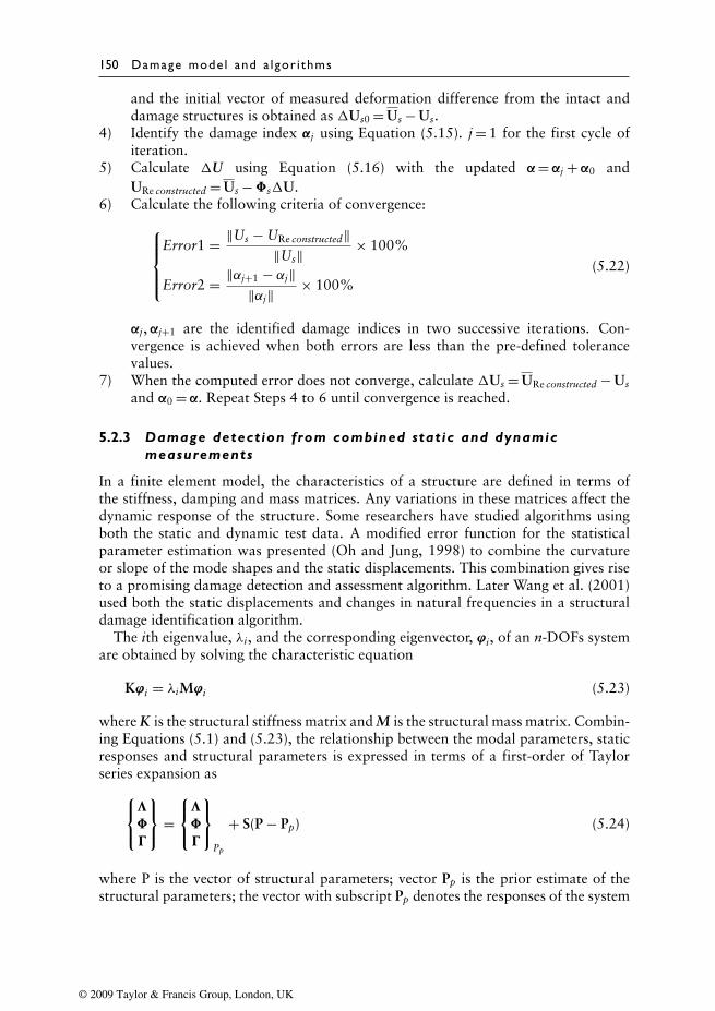
150 Damage mode l and a lgor i thms
and the initial vector of measured deformation difference from the intact anddamage structures is obtained as �Us0 = Us − Us.
4) Identify the damage index αj using Equation (5.15). j = 1 for the first cycle ofiteration.
5) Calculate �U using Equation (5.16) with the updated α = αj + α0 andURe constructed = Us − �s�U.
6) Calculate the following criteria of convergence:Error1 = ‖Us − URe constructed‖
‖Us‖ × 100%
Error2 = ‖αj+1 − αj‖‖αj‖ × 100%
(5.22)
αj, αj+1 are the identified damage indices in two successive iterations. Con-vergence is achieved when both errors are less than the pre-defined tolerancevalues.
7) When the computed error does not converge, calculate �Us = URe constructed − Us
and α0 = α. Repeat Steps 4 to 6 until convergence is reached.
5.2.3 Damage detection from combined static and dynamicmeasurements
In a finite element model, the characteristics of a structure are defined in terms ofthe stiffness, damping and mass matrices. Any variations in these matrices affect thedynamic response of the structure. Some researchers have studied algorithms usingboth the static and dynamic test data. A modified error function for the statisticalparameter estimation was presented (Oh and Jung, 1998) to combine the curvatureor slope of the mode shapes and the static displacements. This combination gives riseto a promising damage detection and assessment algorithm. Later Wang et al. (2001)used both the static displacements and changes in natural frequencies in a structuraldamage identification algorithm.
The ith eigenvalue, λi, and the corresponding eigenvector, ϕi, of an n-DOFs systemare obtained by solving the characteristic equation
Kϕi = λiMϕi (5.23)
where K is the structural stiffness matrix and M is the structural mass matrix. Combin-ing Equations (5.1) and (5.23), the relationship between the modal parameters, staticresponses and structural parameters is expressed in terms of a first-order of Taylorseries expansion as
�
=
�
Pp
+ S(P − Pp) (5.24)
where P is the vector of structural parameters; vector Pp is the prior estimate of thestructural parameters; the vector with subscript Pp denotes the responses of the system
© 2009 Taylor & Francis Group, London, UK
Damage detect ion from stat i c measurement 151
when the parameters P = Pp; is the vector of measured eigenvalues; and � and arevectors of dynamic and static error responses, respectively. Let nr be the total numberof responses for the target structure, and S be the partial derivative or sensitivity matrixof the eigenvalues and dynamic and static error responses. It can be written as
S =[∂
∂pj
∂�
∂pj
∂
∂pj
]T
(5.25)
The different types of responses in Equation (5.24) are combined to form the errorfunction. To prevent the case where the contribution of a special response type isreduced due to a relatively small magnitude of the response, an adjusted dynamicresponse should be defined. Therefore, when the combined data of static and modaltests are used in the identification procedure, the measured mode shapes are weightedso that the maximum values of each type of response are the same.
It is noted from Equation (5.24) that the number of structural parameters is not thesame as the number of measured responses, such that the inverse matrix of S does notalways exist. Therefore, an estimate T on such an inverse can be defined as
�p = T�R (5.26)
where �R =
�
−
�
pp
.
The objective of this procedure is to find the best unbiased estimator, �p, based onmeasured values of , � and and prior estimates of the structural parameters, pp.A scalar performance error function in the Bayesian estimation theory is defined forthe derivation of the statistical system identification formula as
E = (R − Rk)TWr(R − Rk) + (P∗k − Pk)TWp(P∗
k − Pk) (5.27)
where Wr and Wp are the weighting matrices for the measured responses and the struc-tural parameters, respectively, which can be assumed as the inverse of the covariancematrices of the errors on the measured responses and the initial structural parameters,respectively; R is the measured responses; Rk, Pk are predicted vectors of responses andstructural parameters, respectively, at the k-th step; and P∗
k is the vector of objectiveparameters.
Other error functions can also be used to estimate the structural parameters. Thechanges in curvatures are local in nature and hence can be used to detect and locatethe damage in the structure. The differences in the curvatures of mode shapes can beused to form the error response vector as well as for estimating the uncertainty ofthe structural parameters. Certainly, the slope of mode shapes is also another possiblecandidate for formulating the error response vectors.
© 2009 Taylor & Francis Group, London, UK
152 Damage mode l and a lgor i thms
5.3 Variation of static deflection profile with damage
5.3.1 The static deflect ion profi le
In Section 5.2, an equivalent scalar parameter is used to describe the variationin the stiffness parameter of a structural element. This approach can determinechanges in structural element stiffness, including failure in an element. The identi-fied cross-sectional properties of the structural elements can be taken as parametersfor assessment and to determine the load-carrying capacity of the structure. In a realcase, the presence of damage in a continuous body is represented by a reduction insome physical parameters of the material in an appropriate constitutive model. In thecase of damage caused by the presence of a crack, it is well known that, besides thestress concentration occurring at the crack tip, there is a zone, adjacent to the crack,denoted as ‘ineffective’ in view of its low stress level. If a straight beam is subjectedto concentrated damage, such as a crack or a saw cut at a certain cross-section, thepresence of the ineffective zone in the crack vicinity can be accounted for by a loss ofthe flexural stiffness in the Euler–Bernoulli beam theory.
The variation in a stiffness parameter can also be modelled as a distribution functionin the structural element, such as modelling the concentrated damages as Dirac’s deltadistribution in the flexural stiffness (Di Paola and Bilello, 2004; Caddemi and Greco,2006; Buda and Caddemi, 2007). Basically, the presence of damage can be representedthrough a variation of its bending stiffness as
EI(x, xd, βd) = EI × [(1 − d(x, xd, βd))] (5.28)
where EI is the bending stiffness of the undamaged beam; d(x, xd, βd) is the damage dis-tribution function; while xd, βd are q-dimensional vectors (q is the number of damageevents) of damage locations and extent, respectively. The upper bound of the damagedistribution function, d(x, xd, βd) = 0, corresponds to the undamaged case while thelower bound, d(x, xd, βd) = 1, indicates a local failure due to damage. For a concen-trated crack, d(x, xd,βd) =βdδ(x − xd), δ(x − xd) is a Dirac’s delta distribution centredat xd.
The static equations of an Euler–Bernoulli beam subjected to the external load f (x)are easily obtained in the form
Q′(x) = −f (x)
M′(x) = Q(x)
ϕ(x) = −u′(x) (5.29)
χ′(x) = ϕ′(x)
χ(x) = M(x)/EI(x, xd, βd)
where f (x) is the external vertical load; Q(x) and M(x) are the shear force and thebending moment, respectively; u(x),ϕ(x),χ(x) are the deflection, slope and curvaturefunctions, respectively; and the prime denotes differentiation with respect to the spatialcoordinate x, spanning from 0 to the length L of the beam. The first four equations inEquation (5.29) are the equilibrium and compatibility equations, and the final one is
© 2009 Taylor & Francis Group, London, UK
Damage detect ion from stat i c measurement 153
the constitutive equation relating curvature and bending moment through the spatialvariable flexural stiffness EI(x).
Combining the equilibrium, the compatibility and the constitutive equations yieldsthe following fourth-order differential governing equation in the beam deflectiontheory as
[EI(x, xd, βd)u′′(x)]′′ = f (x) (5.30)
With the presence of a local damage, the fourth-order governing differential equationis obtained as
{EI[1 − βdδ(x − xd)]u′′(x)}′′ = f (x) (5.31)
The deflection function, u(x), can be obtained by integrating the governing equationof the Euler–Bernoulli beam as
u(x) = c4 + c3x + c1
2EI[x2 + 2
βd
1 − βaA(x − xd)U(x − xd)] + C2
6EI
× [x3 + 6βd
1 − βdAU(x − xd)] + f [4](x)
EI
+ βd
1 − βdAf [2](xd)
EI(x − xd)U(x − xd) (5.32)
where U(x − xd) is the unit step distribution, also called the Heaviside function.It represents the formal primitive of the Dirac’s delta with discontinuity at xd,U(x − xd) = 0 for x< xd and U(x − xd) = 1 for x ≥ xd. Constants c1, c2, c3 and c4
can be obtained by the enforcement of boundary conditions; f [k](x) denotes a prim-itive of order of the external load function, f (x); and A is a constant defined asAδ(x − xd) = δ(x − xd)δ(x − xd) (Bagarello, 1995).
According to the explicit solutions of the response in terms of the crack positionand intensity, the damage parameters can be identified by means of the followingminimization problem
J(xd, βd) = 12
nlc∑i=1
nm∑j=1
wi[ui(xj, xd, βd) − uei (xj)]2 (5.33)
or
J(xd, βd) = 12
nlc∑i=1
nm∑j=1
wi[�ui(xj, xd, βd) −�uei (xj)]2 (5.34)
where wi is the weight associated with the ith load case; nlc is the number of loadcases; nm is the number of measurements; ui(xj, xd, βd), ue
i (xj) are the theoretical andexperimental measured deflection at nm different cross-sections for nlc load cases,respectively; and�ui(xj, xd, βd),�ue
i (xj) are the theoretical and experimental measuredvariations of a structural response due to damage, respectively.
© 2009 Taylor & Francis Group, London, UK
154 Damage mode l and a lgor i thms
5.3.2 Spatial wavelet transform
From the above discussion, the closed form deflection can be written in terms of thedamage intensities and positions. The local damage is treated as an abnormal flexuralstiffness that induces some singularity in the deflection function.
An important feature of the wavelet transform is its ability to characterize the localirregularity of a function and its sensitivity to small changes in the structure. A crackin a structure introduces singularities to the dynamic displacement mode shapes andthe static deflection profile. These small changes cannot be identified directly from thestructural response, but they may be observed in the wavelet transforms since localabnormalities in the signal would result in large wavelet coefficients in the proximityof the damage. The applicability of the wavelet damage detection techniques dependson the measurement precision and the sensor spacing.
With the development of modern sensor technology, the measurement of the beamdisplacements at a large number of spatially distributed points can be obtained byprocessing digital photographs of the beams (Rucka and Wilde, 2006). The high-resolution camera equipped with a metric optic matrix that allows precise mapping of3D objects into 2D digital photographs is also a means to obtain high quality data.Recently, the operational deflection of a bridge deck under moving loads is used fordamage assessment (Zhu and Law, 2006). The study shows that the response at a singlepoint from the passage of a very slow moving load is equivalent to the displacementof the whole bridge deck loaded at the measuring point. This method will be studiedin detail in Section 8.2.
5.4 Application
5.4.1 Damage assessment of concrete beams
5.4.1.1 Ef fec t o f measurement no i se
A numerical example with a four-metre long simply supported uniform rectangularconcrete beam is studied. It has a 300 mm high and 200 mm wide cross-section and3.8 m clear span. There are three 20 mm diameter mild steel bars at the bottom of thebeam corresponding to a steel percentage of 1.57%, and two 6 mm diameter steel barsat the top of the beam section. Mild steel links with a 6 mm diameter are provided at195 mm spacing over the whole beam length. The density, tensile strength, elastic mod-ulus and Poisson’s Ratio of concrete are 2351.4 kg/m3, 3.77 MPa, 30.2 GPa and 0.16,respectively. The elastic modulus and yield stress of the mild steel bars are 181.53 GPaand 300.07 MPa, respectively.
One per cent white noise is added to the calculated displacements of the beam tosimulate the polluted measurements with
U s = U calculated(1 + Ep · Nnoise) (5.35)
where Us and Ucalculated are the polluted and the original ‘measured’ displacements; Ep
is the noise level; and Nnoise is a standard normally distributed vector with zero meanand unit standard deviation, and it is generated independently for each component ofthe measured displacement.
© 2009 Taylor & Francis Group, London, UK
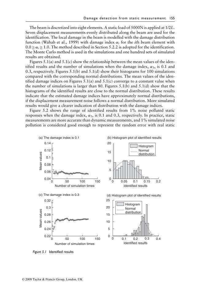
Damage detect ion from stat i c measurement 155
The beam is discretized into eight elements. A static load of 5000N is applied at 1/2L.Seven displacement measurements evenly distributed along the beam are used for theidentification. The local damage in the beam is modelled with the damage distributionfunction (Wahab et al., 1999) with damage index αi for the ith beam element with0.0 ≥αi ≥ 1.0. The method described in Section 5.2.2 is adopted for the identification.The Monte Carlo method is used in the simulations and one hundred sets of simulatedresults are obtained.
Figures 5.1(a) and 5.1(c) show the relationship between the mean values of the iden-tified results and the number of simulations when the damage index, α3, is 0.1 and0.3, respectively. Figures 5.1(b) and 5.1(d) show their histograms for 100 simulationscompared with the corresponding normal distributions. The mean values of the iden-tified damage indices on Figures 5.1(a) and 5.1(c) converge to a constant value whenthe number of simulations is larger than 80. Figures 5.1(b) and 5.1(d) show that thehistograms of the identified results are close to the normal distribution. These resultsindicate that the estimated damage indices have approximately normal distributions,if the displacement measurement noise follows a normal distribution. More simulatedresults would give a clearer indication of distribution with the damage indices.
Figure 5.2 shows the range of identified results from 1% noise polluted staticresponses when the damage index, α3, is 0.1 and 0.3, respectively. In practice, staticmeasurements are more accurate than dynamic measurements, and 1% simulated noisepollution is considered good enough to represent the random error with real static
0 50 100 1500.04
0.06
0.08
0.1
0.12
0.14
Mea
n va
lues
(a) The damage index is 0.1
Number of simulation times0 0.05 0.1 0.15 0.2
0
5
10
15
20
(b) Histogram plot of identified results
Identified results
0 50 100 1500.22
0.24
0.26
0.28
0.3
0.32
Mea
n va
lues
(c) The damage index is 0.3
Number of simulation times
0 0.1 0.2 0.3 0.40
5
10
15
20
25
(d) Histogram plot of identified results
Identified results
HistogramNormaldistribution
HistogramNormaldistribution
Figure 5.1 Identified results
© 2009 Taylor & Francis Group, London, UK
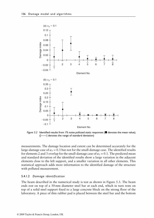
156 Damage mode l and a lgor i thms
�0.04
�0.02
0
0.02
0.04
0.06
0.08
0.1
0.12
Element No.
Dam
age
inde
x
�0.1
�0.05
0
12 3 4 5 6 7 8
12 3 4 5 6 7 8
0.05
0.1
0.15
0.2
0.25
0.3
0.35
Element No.
Dam
age
inde
x
(a) α3 � 0.1
(b) α3 � 0.1
Figure 5.2 Identified results from 1% noise polluted static responses (� denotes the mean value),(|——| denotes the range of standard deviation)
measurements. The damage location and extent can be determined accurately for thelarge-damage case of α3 = 0.3 but not for the small-damage case. The identified resultsfor elements 2 and 3 overlap for the small-damage case of α3 = 0.1. The predicted meanand standard deviation of the identified results show a large variation in the adjacentelements close to the left support, and a smaller variation in all other elements. Thisstatistical approach adds more information to the identified damage of the structurewith polluted measurement.
5.4.1.2 Damage ident i f i cat ion
The beam described in the numerical study is test as shown in Figure 5.3. The beamends rest on top of a 50 mm diameter steel bar at each end, which in turn rests ontop of a solid steel support fixed to a large concrete block on the strong floor of thelaboratory. A piece of thin rubber pad is placed between the steel bar and the bottom
© 2009 Taylor & Francis Group, London, UK
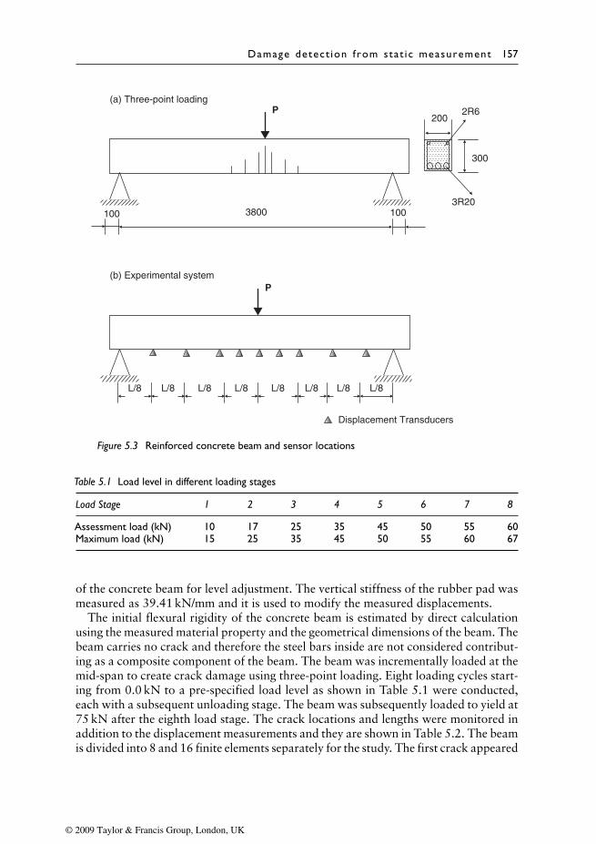
Damage detect ion from stat i c measurement 157
(a) Three-point loading2R6
3R20
200
300
3800 100100
P
Displacement Transducers
(b) Experimental system P
L/8 L/8 L/8 L/8 L/8 L/8 L/8 L/8
Figure 5.3 Reinforced concrete beam and sensor locations
Table 5.1 Load level in different loading stages
Load Stage 1 2 3 4 5 6 7 8
Assessment load (kN) 10 17 25 35 45 50 55 60Maximum load (kN) 15 25 35 45 50 55 60 67
of the concrete beam for level adjustment. The vertical stiffness of the rubber pad wasmeasured as 39.41 kN/mm and it is used to modify the measured displacements.
The initial flexural rigidity of the concrete beam is estimated by direct calculationusing the measured material property and the geometrical dimensions of the beam. Thebeam carries no crack and therefore the steel bars inside are not considered contribut-ing as a composite component of the beam. The beam was incrementally loaded at themid-span to create crack damage using three-point loading. Eight loading cycles start-ing from 0.0 kN to a pre-specified load level as shown in Table 5.1 were conducted,each with a subsequent unloading stage. The beam was subsequently loaded to yield at75 kN after the eighth load stage. The crack locations and lengths were monitored inaddition to the displacement measurements and they are shown in Table 5.2. The beamis divided into 8 and 16 finite elements separately for the study. The first crack appeared
© 2009 Taylor & Francis Group, London, UK
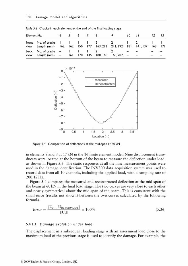
158 Damage mode l and a lgor i thms
Table 5.2 Cracks in each element at the end of the final loading stage
Element No. 4 5 6 7 8 9 10 11 12 13
front No. of cracks 1 1 1 1 2 2 1 2 1 1view Length (mm) 162 162 150 177 163, 211 211, 192 181 141, 137 163 171back No. of cracks – 1 1 1 2 2 – – – –view Length (mm) – 161 170 145 180, 160 160, 202 – – – –
0 0.5 1 1.5 2 2.5 3 3.5�9
�8
�7
�6
�5
�4
�3
�2
�1
0� 10�3
Location (m)
Def
lect
ion
(m)
MeasuredReconstructed
Figure 5.4 Comparison of deflections at the mid-span at 60 kN
in elements 8 and 9 at 17 kN in the 16 finite element model. Nine displacement trans-ducers were located at the bottom of the beam to measure the deflection under load,as shown in Figure 5.3. The static responses at all the nine measurement points wereused in the damage identification. The INV300 data acquisition system was used torecord data from all 10 channels, including the applied load, with a sampling rate of200.12 Hz.
Figure 5.4 compares the measured and reconstructed deflection at the mid-span ofthe beam at 60 kN in the final load stage. The two curves are very close to each otherand nearly symmetrical about the mid-span of the beam. This is consistent with thesmall error (results not shown) between the two curves calculated by the followingformula.
Error = ‖Us − URe constructed‖‖Us‖ × 100% (5.36)
5.4.1.3 Damage evo lut ion under load
The displacement in a subsequent loading stage with an assessment load close to themaximum load of the previous stage is used to identify the damage. For example, the
© 2009 Taylor & Francis Group, London, UK
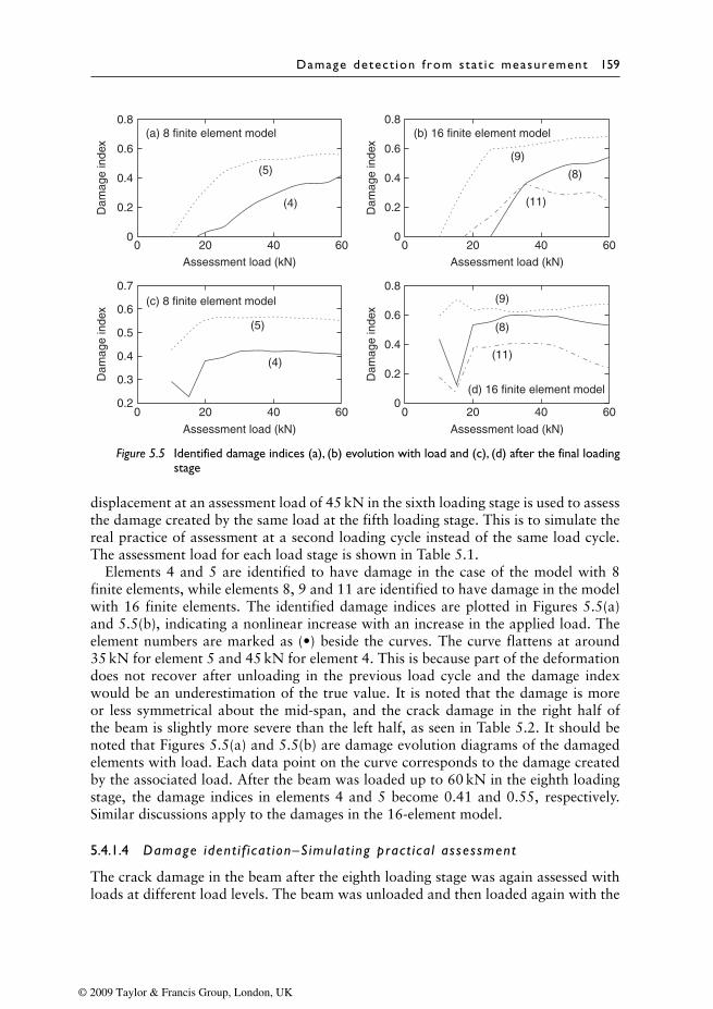
Damage detect ion from stat i c measurement 159
00 20
Assessment load (kN)
(a) 8 finite element model
(c) 8 finite element model
(b) 16 finite element model
(d) 16 finite element model
Dam
age
inde
x
Dam
age
inde
x
Dam
age
inde
x
Dam
age
inde
x
Assessment load (kN)
Assessment load (kN)Assessment load (kN)
40
(5)
(5)
(4)
(4)
(9)
(9)
(8)
(11)
(8)
(11)
60 0 20 40 60
0 20 40 600 20 40 600.2
0.3
0.4
0.5
0.6
0.7
0.2
0.4
0.6
0.8
0
0.2
0.4
0.6
0.8
0
0.2
0.4
0.6
0.8
Figure 5.5 Identified damage indices (a), (b) evolution with load and (c), (d) after the final loadingstage
displacement at an assessment load of 45 kN in the sixth loading stage is used to assessthe damage created by the same load at the fifth loading stage. This is to simulate thereal practice of assessment at a second loading cycle instead of the same load cycle.The assessment load for each load stage is shown in Table 5.1.
Elements 4 and 5 are identified to have damage in the case of the model with 8finite elements, while elements 8, 9 and 11 are identified to have damage in the modelwith 16 finite elements. The identified damage indices are plotted in Figures 5.5(a)and 5.5(b), indicating a nonlinear increase with an increase in the applied load. Theelement numbers are marked as (•) beside the curves. The curve flattens at around35 kN for element 5 and 45 kN for element 4. This is because part of the deformationdoes not recover after unloading in the previous load cycle and the damage indexwould be an underestimation of the true value. It is noted that the damage is moreor less symmetrical about the mid-span, and the crack damage in the right half ofthe beam is slightly more severe than the left half, as seen in Table 5.2. It should benoted that Figures 5.5(a) and 5.5(b) are damage evolution diagrams of the damagedelements with load. Each data point on the curve corresponds to the damage createdby the associated load. After the beam was loaded up to 60 kN in the eighth loadingstage, the damage indices in elements 4 and 5 become 0.41 and 0.55, respectively.Similar discussions apply to the damages in the 16-element model.
5.4.1.4 Damage ident i f i cat ion–S imulat ing pract i ca l assessment
The crack damage in the beam after the eighth loading stage was again assessed withloads at different load levels. The beam was unloaded and then loaded again with the
© 2009 Taylor & Francis Group, London, UK
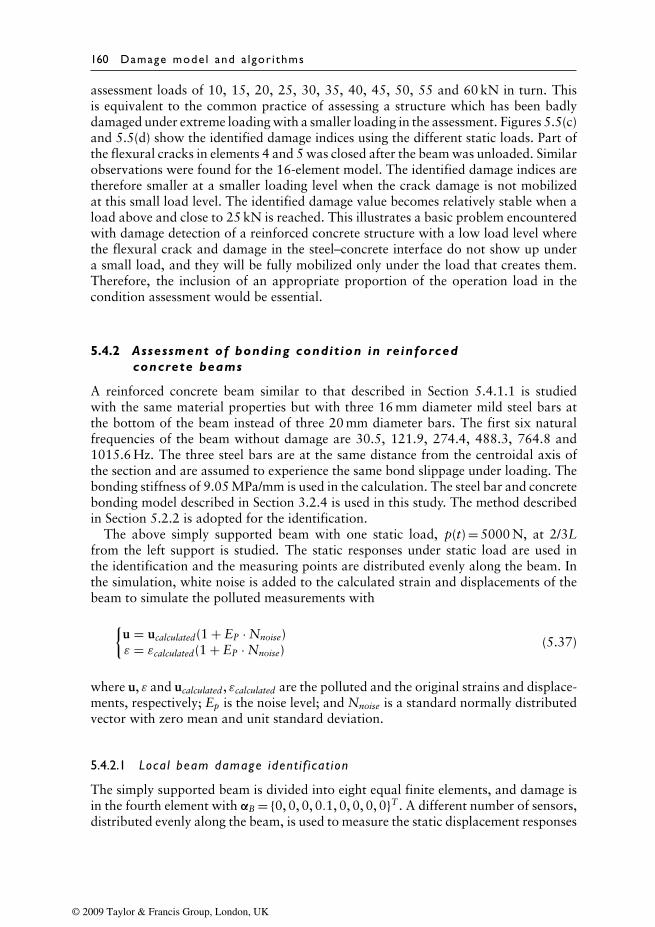
160 Damage mode l and a lgor i thms
assessment loads of 10, 15, 20, 25, 30, 35, 40, 45, 50, 55 and 60 kN in turn. Thisis equivalent to the common practice of assessing a structure which has been badlydamaged under extreme loading with a smaller loading in the assessment. Figures 5.5(c)and 5.5(d) show the identified damage indices using the different static loads. Part ofthe flexural cracks in elements 4 and 5 was closed after the beam was unloaded. Similarobservations were found for the 16-element model. The identified damage indices aretherefore smaller at a smaller loading level when the crack damage is not mobilizedat this small load level. The identified damage value becomes relatively stable when aload above and close to 25 kN is reached. This illustrates a basic problem encounteredwith damage detection of a reinforced concrete structure with a low load level wherethe flexural crack and damage in the steel–concrete interface do not show up undera small load, and they will be fully mobilized only under the load that creates them.Therefore, the inclusion of an appropriate proportion of the operation load in thecondition assessment would be essential.
5.4.2 Assessment of bonding condit ion in reinforcedconcrete beams
A reinforced concrete beam similar to that described in Section 5.4.1.1 is studiedwith the same material properties but with three 16 mm diameter mild steel bars atthe bottom of the beam instead of three 20 mm diameter bars. The first six naturalfrequencies of the beam without damage are 30.5, 121.9, 274.4, 488.3, 764.8 and1015.6 Hz. The three steel bars are at the same distance from the centroidal axis ofthe section and are assumed to experience the same bond slippage under loading. Thebonding stiffness of 9.05 MPa/mm is used in the calculation. The steel bar and concretebonding model described in Section 3.2.4 is used in this study. The method describedin Section 5.2.2 is adopted for the identification.
The above simply supported beam with one static load, p(t) = 5000 N, at 2/3Lfrom the left support is studied. The static responses under static load are used inthe identification and the measuring points are distributed evenly along the beam. Inthe simulation, white noise is added to the calculated strain and displacements of thebeam to simulate the polluted measurements with
{u = ucalculated(1 + EP · Nnoise)ε = εcalculated(1 + EP · Nnoise)
(5.37)
where u, ε and ucalculated, εcalculated are the polluted and the original strains and displace-ments, respectively; Ep is the noise level; and Nnoise is a standard normally distributedvector with zero mean and unit standard deviation.
5.4.2.1 Loca l beam damage ident i f i cat ion
The simply supported beam is divided into eight equal finite elements, and damage isin the fourth element with αB = {0, 0, 0, 0.1, 0, 0, 0, 0}T . A different number of sensors,distributed evenly along the beam, is used to measure the static displacement responses
© 2009 Taylor & Francis Group, London, UK
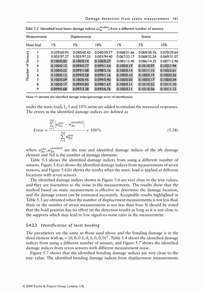
Damage detect ion from stat i c measurement 161
Table 5.3 Identified local beam damage indices (αidentifiedBe ) from a different number of sensors
Measurements Displacements Strains
Noise level 1% 5% 10% 1% 5% 10%
Num
ber
ofSe
nsor
s 1 0.039/60.93 0.040/60.42 0.040/59.77 0.068/31.66 0.069/30.76 0.070/29.642 0.003/97.27 0.003/97.33 0.003/94.40 0.067/33.17 0.068/32.24 0.069/31.073 0.100/0.05 0.100/0.14 0.100/0.27 0.085/15.40 0.086/14.32 0.087/12.964 0.100/0.15 0.099/0.77 0.099/1.54 0.100/0.19 0.101/0.97 0.102/1.945 0.100/0.22 0.099/1.08 0.098/2.16 0.100/0.14 0.101/1.15 0.103/2.616 0.100/0.12 0.099/0.58 0.099/1.16 0.100/0.10 0.100/0.19 0.100/0.367 0.100/0.09 0.100/0.45 0.099/0.90 0.100/0.03 0.100/0.17 0.100/0.348 0.100/0.17 0.099/0.83 0.098/1.67 0.100/0.11 0.101/0.55 0.101/1.109 0.099/0.68 0.097/3.38 0.093/6.76 0.100/0.11 0.101/0.56 0.101/1.12
Note: •/• denotes the identified damage index/percentage error of identification.
under the static load; 1, 5 and 10% noise are added to simulate the measured responses.The errors in the identified damage indices are defined as
Error =
Nd∑i=1
∣∣∣αtrueBei − αidentified
Bei
∣∣∣Nd∑i=1αtrue
Bei
× 100% (5.38)
where αtrueBei ,αidentified
Bei are the true and identified damage indices of the ith damageelement and Nd is the number of damage elements.
Table 5.3 shows the identified damage indices from using a different number ofsensors. Figure 5.6(a) shows the identified damage indices from measurements of sevensensors, and Figure 5.6(b) shows the results when the static load is applied at differentlocations with seven sensors.
The identified damage indices shown in Figure 5.6 are very close to the true values,and they are insensitive to the noise in the measurements. The results show that themethod based on static measurement is effective to determine the damage location,and the damage extent can be estimated accurately. Acceptable results highlighted inTable 5.3 are obtained when the number of displacement measurements is not less thanthree or the number of strain measurements is not less than four. It should be notedthat the load position has no effect on the detection results as long as it is not close tothe supports which may lead to low signal-to-noise ratio in the measurement.
5.4.2.2 Ident i f i cat ion of loca l bond ing
The parameters are the same as those used above and the bonding damage is in thethird element with αb = {0, 0, 0.1, 0, 0, 0, 0, 0}T . Table 5.4 shows the identified damageindices from using a different number of sensors, and Figure 5.7 shows the identifieddamage indices from seven sensors with different measurement noise.
Figure 5.7 shows that the identified bonding damage indices are very close to thetrue value. The identified bonding damage indices from displacement measurements
© 2009 Taylor & Francis Group, London, UK
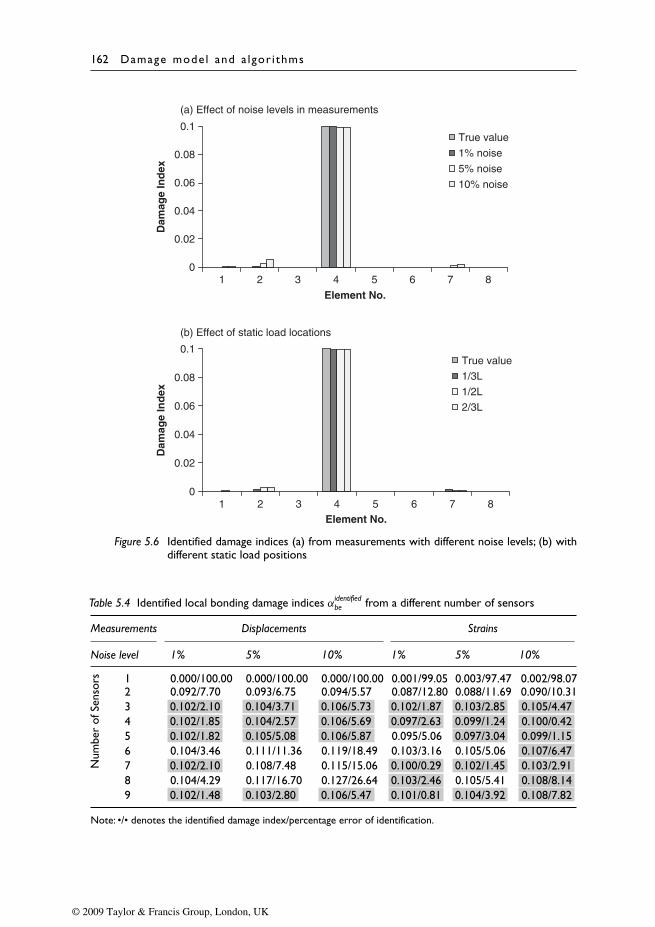
162 Damage mode l and a lgor i thms
0
0.02
0.04
0.06
0.08
0.1
1 2 3 4 5 6 7 8
Element No.
Dam
age
Ind
ex
True value
1% noise
5% noise
10% noise
0
0.02
0.04
0.06
0.08
0.1
1 2 3 4 5 6 7 8Element No.
Dam
age
Ind
ex
True value
1/3L
1/2L
2/3L
(a) Effect of noise levels in measurements
(b) Effect of static load locations
Figure 5.6 Identified damage indices (a) from measurements with different noise levels; (b) withdifferent static load positions
Table 5.4 Identified local bonding damage indices αidentifiedbe from a different number of sensors
Measurements Displacements Strains
Noise level 1% 5% 10% 1% 5% 10%
Num
ber
ofSe
nsor
s 1 0.000/100.00 0.000/100.00 0.000/100.00 0.001/99.05 0.003/97.47 0.002/98.072 0.092/7.70 0.093/6.75 0.094/5.57 0.087/12.80 0.088/11.69 0.090/10.313 0.102/2.10 0.104/3.71 0.106/5.73 0.102/1.87 0.103/2.85 0.105/4.474 0.102/1.85 0.104/2.57 0.106/5.69 0.097/2.63 0.099/1.24 0.100/0.425 0.102/1.82 0.105/5.08 0.106/5.87 0.095/5.06 0.097/3.04 0.099/1.156 0.104/3.46 0.111/11.36 0.119/18.49 0.103/3.16 0.105/5.06 0.107/6.477 0.102/2.10 0.108/7.48 0.115/15.06 0.100/0.29 0.102/1.45 0.103/2.918 0.104/4.29 0.117/16.70 0.127/26.64 0.103/2.46 0.105/5.41 0.108/8.149 0.102/1.48 0.103/2.80 0.106/5.47 0.101/0.81 0.104/3.92 0.108/7.82
Note: •/• denotes the identified damage index/percentage error of identification.
© 2009 Taylor & Francis Group, London, UK
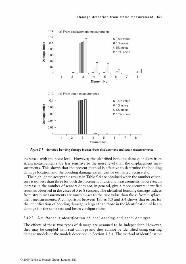
Damage detect ion from stat i c measurement 163
0
0.02
0.04
0.06
0.08
0.1
0.12
0.14
1 2 3 4 5 6 7 8
Element No.
Dam
age
Ind
ex
True value
(a) From displacement measurements
(b) From strain measurements
1% noise
5% noise
10% noise
0
0.02
0.04
0.06
0.08
0.1
0.12
1 2 3 4 5 6 7 8
Element No.
Dam
age
Ind
ex
True value
1% noise
5% noise
10% noise
Figure 5.7 Identified bonding damage indices from displacement and strain measurements
increased with the noise level. However, the identified bonding damage indices fromstrain measurements are less sensitive to the noise level than the displacement mea-surements. This shows that the present method is effective to determine the bondingdamage location and the bonding damage extent can be estimated accurately.
The highlighted acceptable results in Table 5.4 are obtained when the number of sen-sors is not less than three for both displacement and strain measurements. However, anincrease in the number of sensors does not, in general, give a more accurate identifiedresult as observed in the cases of 5 to 8 sensors. The identified bonding damage indicesfrom strain measurements are much closer to the true value than those from displace-ment measurements. A comparison between Tables 5.3 and 5.4 shows that errors forthe identification of bonding damage is larger than those in the identification of beamdamage for the same test and beam configurations.
5.4.2.3 S imul taneous ident i f i cat ion of loca l bond ing and beam damages
The effects of these two types of damage are assumed to be independent. However,they may be coupled with real damage and they cannot be identified using existingdamage models or the models described in Section 3.2.4. The method of identification
© 2009 Taylor & Francis Group, London, UK
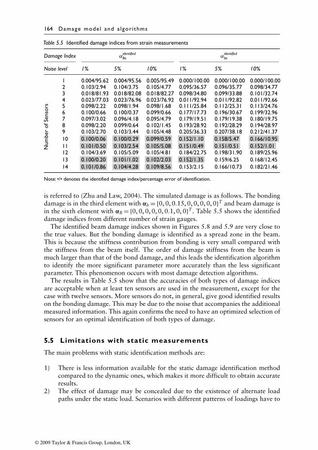
164 Damage mode l and a lgor i thms
Table 5.5 Identified damage indices from strain measurements
Damage Index αidentifiedBe α
identifiedbe
Noise level 1% 5% 10% 1% 5% 10%
1 0.004/95.62 0.004/95.56 0.005/95.49 0.000/100.00 0.000/100.00 0.000/100.002 0.103/2.94 0.104/3.75 0.105/4.77 0.095/36.57 0.096/35.77 0.098/34.773 0.018/81.93 0.018/82.08 0.018/82.27 0.098/34.80 0.099/33.88 0.101/32.744 0.023/77.03 0.023/76.96 0.023/76.92 0.011/92.94 0.011/92.82 0.011/92.66
Num
ber
ofSe
nsor
s 5 0.098/2.22 0.098/1.94 0.098/1.68 0.111/25.84 0.112/25.31 0.113/24.766 0.100/0.66 0.100/0.37 0.099/0.66 0.177/17.73 0.196/30.67 0.199/32.967 0.097/3.02 0.096/4.18 0.095/4.79 0.179/19.51 0.179/19.38 0.180/19.758 0.098/2.20 0.099/0.64 0.102/1.45 0.193/28.92 0.192/28.29 0.194/28.979 0.103/2.70 0.103/3.44 0.105/4.48 0.205/36.33 0.207/38.18 0.212/41.3710 0.100/0.06 0.100/0.29 0.099/0.59 0.152/1.10 0.158/5.47 0.166/10.9511 0.101/0.50 0.103/2.54 0.105/5.08 0.151/0.49 0.151/0.51 0.152/1.0112 0.104/3.69 0.105/5.09 0.105/4.81 0.184/22.75 0.198/31.90 0.189/25.9613 0.100/0.20 0.101/1.02 0.102/2.03 0.152/1.35 0.159/6.25 0.168/12.4514 0.101/0.86 0.104/4.28 0.109/8.56 0.153/2.15 0.166/10.73 0.182/21.46
Note: •/• denotes the identified damage index/percentage error of identification.
is referred to (Zhu and Law, 2004). The simulated damage is as follows. The bondingdamage is in the third element with αb = {0, 0, 0.15, 0, 0, 0, 0, 0}T and beam damage isin the sixth element with αB = {0, 0, 0, 0, 0, 0.1, 0, 0}T . Table 5.5 shows the identifieddamage indices from different number of strain gauges.
The identified beam damage indices shown in Figures 5.8 and 5.9 are very close tothe true values. But the bonding damage is identified as a spread zone in the beam.This is because the stiffness contribution from bonding is very small compared withthe stiffness from the beam itself. The order of damage stiffness from the beam ismuch larger than that of the bond damage, and this leads the identification algorithmto identify the more significant parameter more accurately than the less significantparameter. This phenomenon occurs with most damage detection algorithms.
The results in Table 5.5 show that the accuracies of both types of damage indicesare acceptable when at least ten sensors are used in the measurement, except for thecase with twelve sensors. More sensors do not, in general, give good identified resultson the bonding damage. This may be due to the noise that accompanies the additionalmeasured information. This again confirms the need to have an optimized selection ofsensors for an optimal identification of both types of damage.
5.5 Limitations with static measurements
The main problems with static identification methods are:
1) There is less information available for the static damage identification methodcompared to the dynamic ones, which makes it more difficult to obtain accurateresults.
2) The effect of damage may be concealed due to the existence of alternate loadpaths under the static load. Scenarios with different patterns of loadings have to
© 2009 Taylor & Francis Group, London, UK
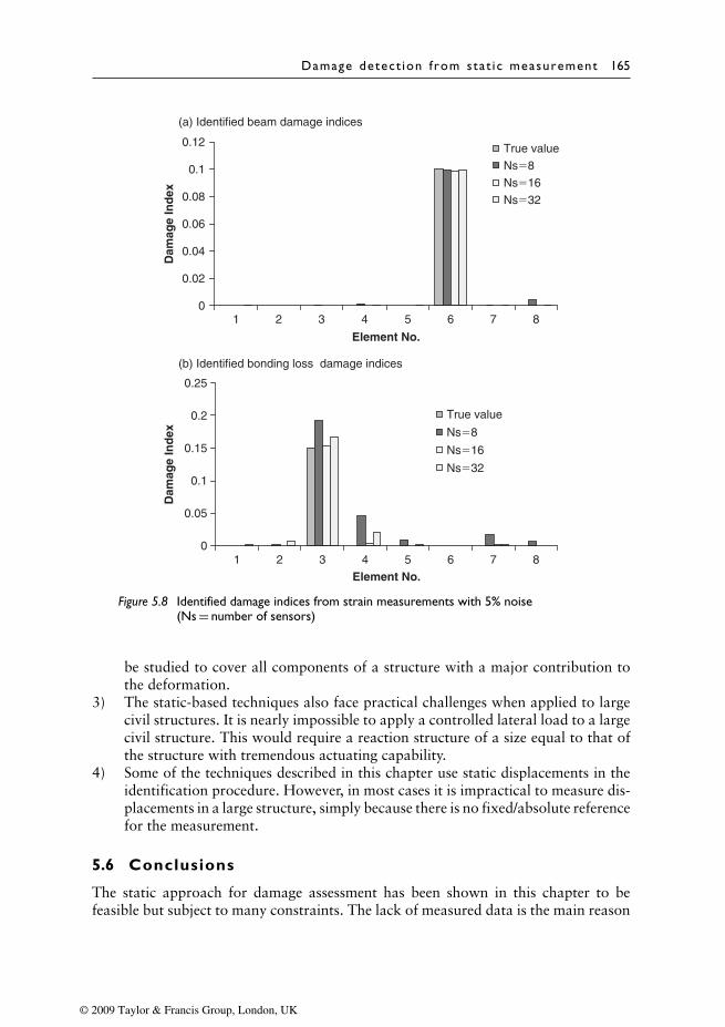
Damage detect ion from stat i c measurement 165
0
0.02
0.04
0.06
0.08
0.1
0.12
1 2 3 4 5 6 7 8
Element No.
Dam
age
Ind
ex
True value
Ns�8
Ns�16
Ns�32
0
0.05
0.1
0.15
0.2
0.25
1 2 3 4 5 6 7 8
Element No.
Dam
age
Ind
ex
True value
Ns�8
Ns�16
Ns�32
(a) Identified beam damage indices
(b) Identified bonding loss damage indices
Figure 5.8 Identified damage indices from strain measurements with 5% noise(Ns = number of sensors)
be studied to cover all components of a structure with a major contribution tothe deformation.
3) The static-based techniques also face practical challenges when applied to largecivil structures. It is nearly impossible to apply a controlled lateral load to a largecivil structure. This would require a reaction structure of a size equal to that ofthe structure with tremendous actuating capability.
4) Some of the techniques described in this chapter use static displacements in theidentification procedure. However, in most cases it is impractical to measure dis-placements in a large structure, simply because there is no fixed/absolute referencefor the measurement.
5.6 Conclusions
The static approach for damage assessment has been shown in this chapter to befeasible but subject to many constraints. The lack of measured data is the main reason
© 2009 Taylor & Francis Group, London, UK
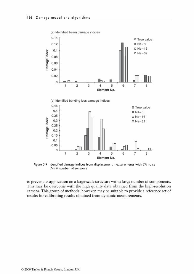
166 Damage mode l and a lgor i thms
0
0.02
0.04
0.06
0.08
0.1
0.12
0.14
1 2 3 4 5 6 7 8Element No.
Dam
age
Ind
ex
True value
Ns�8
Ns�16
Ns�32
0
0.05
0.1
0.15
0.2
0.25
0.3
0.35
0.4
0.45
1 2 3 4 5 6 7 8Element No.
Dam
age
Ind
ex
True value
Ns�8
Ns�16
Ns�32
(a) Identified beam damage indices
(b) Identified bonding loss damage indices
Figure 5.9 Identified damage indices from displacement measurements with 5% noise(Ns = number of sensors)
to prevent its application on a large-scale structure with a large number of components.This may be overcome with the high quality data obtained from the high-resolutioncamera. This group of methods, however, may be suitable to provide a reference set ofresults for calibrating results obtained from dynamic measurements.
© 2009 Taylor & Francis Group, London, UK
Chapter 6
Damage detection in thefrequency domain
6.1 Introduction
Static methods have been discussed in Chapter 5 to identify local damage from staticstructural responses. Similar to the static methods, the vibration-based technique is alsoan attractive alternative for structural damage detection, and many researchers havemade great efforts to advance knowledge in this area. The basic idea of the vibration-based technique is to measure the dynamic characteristics at some specific stages overthe life span of the structure, and use them as a database to assess the condition of thestructure.
This chapter discusses this group of vibration-based structural damage assessmenttechniques. The basic concept of modal analysis is firstly introduced in Section 6.2and the mathematical theory of the eigenvalue problem is presented in Section 6.3.Based on the sensitivity of the eigenvalue and eigenvector, a non-destructive damagedetection algorithm is presented in Section 6.4. To further increase the sensitivity ofmodal responses to the local change in stiffness or mass properties, the high-ordermodal parameters, such as the element modal strain energy, modal flexibility and unitload surface are introduced in Section 6.6, and their curvature in the spatial domainare presented in Section 6.7.
6.2 Spatial distributed system
The dynamics of a structure are physically decomposed by frequency and position.This is clearly evidenced by the analytical solution of partial differential equations ofcontinuous systems such as beams and strings. Modal analysis is based on the fact thatthe vibration response of a linear time-invariant dynamic system can be expressed asthe linear combination of a set of simple harmonic motions called the natural modesof vibration. The natural modes of vibration are inherent to a dynamic system and aredetermined completely by its physical properties (mass, stiffness, damping) and theirspatial distributions. Each mode is described in terms of its modal parameters: naturalfrequency, modal damping factor and the characteristic displacement pattern, calledthe mode shape. The mode shape may be real or complex with each one correspondingto a natural frequency. The degree of participation of each natural mode in the overallvibration is determined both by the properties of the excitation sources and by themode shapes of the system.
© 2009 Taylor & Francis Group, London, UK
168 Damage mode ls and a lgor i thms
Modal analysis embraces both theoretical and experimental techniques. The theo-retical modal analysis is based on the physical model of a dynamic system comprisingits mass, stiffness and damping properties. These properties may be in the form ofpartial differential equations. An example is the wave equation of a uniform vibratorystring established from its mass distribution and elasticity properties. The solution ofthe equation provides the natural frequencies and mode shapes of the string and itsforced vibration responses. However, a more realistic physical model will usually com-prise the mass, stiffness and damping properties in terms of their spatial distributions,namely the mass, stiffness and damping matrices. These matrices are incorporated intoa set of normal differential equations of motion. The superposition principle of a lin-ear dynamic system enables us to transform these equations into a typical eigenvalueproblem, the solution of which provides the modal information of the system. Mod-ern finite element analysis empowers the discretization of almost any linear dynamicstructure and hence has greatly enhanced the capacity and scope of theoretical modalanalysis. However, the rapid development over the last two decades of data acquisitionand processing capabilities has given rise to major advances in the experimental realmof the analysis, which has become known as modal testing.
6.3 The eigenvalue problem
6.3.1 Sensit iv ity of eigenvalues and eigenvectors
The real symmetric eigenvalue problem associated with linear vibration is defined as
Kφj = λjMφj (6.1)
where K and M are the stiffness and mass matrices, and they are of order n symmetricmatrices. M is positive definite and K is positive definite or semi-positive definite.Eigenvector, φj, is the jth mode shape and eigenvalue, λj, is the square of the jthnatural frequency. The eigenvector, φj, is typically normalized as
φjMφj = 1 (6.2)
To obtain the derivative of the eigenvalue, Equation (6.1) is differentiated withrespect to a system parameter, p, as
(K − λjM)∂φj
∂p= −
(∂K∂p
− λj∂M∂p
)φj + ∂λj
∂pMφj (6.3)
Pre-multiplying both sides of Equation (6.3) with φTj
, the eigenvalue derivative isgiven by
∂λj
∂p= φT
j
(∂K∂p
− λj∂M∂p
)φj (6.4)
Since the matrix, (K − λjM), is singular, the eigenvector derivative, ∂φj/∂p, cannot befound directly from Equation (6.3). Nelson (1976) proposed an algorithm expressing
© 2009 Taylor & Francis Group, London, UK
Damage detect ion in the frequency domain 169
the eigenvector derivative in terms of a particular solution, v, and a homogeneoussolution, cφj, as
∂φj
∂p= v + cφj (6.5)
where c is an undetermined coefficient. The particular solution is found by identifyingthe component of the jth eigenvector with the largest absolute value and constrainingits derivative to zero. The undetermined coefficient can be obtained by substitutingEquation (6.5) into the derivative of Equation (6.2) to give
cj = −vTMφj − 0.5φTj∂M∂pφj (6.6)
Nelson’s method is powerful for computing the eigenvector derivatives of general realmatrices with distinct eigenvalues, because it only requires knowledge of the eigenpairsthat are to be differentiated. However, the algorithm of the method is lengthy andcomplicated. For a large-scale system, there may be thousands of degrees-of-freedom(DOFs). In this case, only a few of the first lower modes are calculated, while the otherhigher modes are truncated. Assuming that the first k modes are available with theother (n − k) modes truncated, an eigenvector derivative can be written as (Lee andJung, 1997a)
∂φj
∂p=
k∑i=1
cφi (6.7)
where ci =
1λi − λj
φTi fj, i = j
hj, i = j, fj = −
(∂K∂p
− λj∂M∂p
)φj + ∂λj
∂pMφj and
hj = −0.5φTj Mφj.
A pseudostatic term is added to the expansion of Equation (6.7) to obtain theeigenvector derivative as (Wang, 1985)
∂φj
∂p= K−1
[−(∂K∂p
− λj∂M∂p
)φj + ∂λj
∂pMφj
]+∑
i
diφi (6.8)
Rudisill (1974) proposed an exact solution method solving an unsymmetric linearalgebraic equation with an additional condition. Rewriting Equation (6.1) into
(K − λjM)φj = 0 (6.9)
rearranging Equation (6.3)
(K − λjM)∂φj
∂p− ∂λj
∂pMφj = −
(∂K∂p
− λj∂M∂p
)φj (6.10)
© 2009 Taylor & Francis Group, London, UK
170 Damage mode ls and a lgor i thms
and imposing the constraint on the length of the eigenvectors,
φTj φj = 1 (6.11)
Differentiating Equation (6.11) with respect to the parameter gives
ϕTj
∂ϕj
∂p= 0 (6.12)
Equations (6.9) and (6.12) can be written as a single matrix equation as follows
[φT
j 0K − λjM −Mφj
]∂φj
∂p∂λj
∂p
=
0
−(∂K∂p
− λj∂M∂p
)φj (6.13)
The derivatives ∂φj/∂p and ∂λj/∂p can be found by solving Equation (6.13). Thealgorithm of this method is simple and compact. However, the demand on computerstorage and CPU time is high, since the method has to deal with the unsymmetriccoefficient matrix to find the eigenpair derivative. For the symmetric coefficient matrix,an equation can be obtained similar to Equation (6.10) by differentiating the massnormalized Equation (6.2) with respect to the parameter, and rearranging to give
φTj M∂φj
∂p+ 0.5φT
j∂M∂pφj = 0 (6.14)
Combining Equations (6.10) and (6.14) as a single matrix equation, the derivatives∂φj/∂p and ∂λj/∂p can be found as
[K − λjM −Mφj
−φTj M 0
]∂φj
∂p∂λj
∂p
=
−(∂K∂p
− λj∂M∂p
)φj
0.5φTj∂M∂pφj
(6.15)
6.3.2 System with close or repeated eigenvalues
When there are multiple eigenvalues and a parameter is perturbed, the eigenvectors willbe split into as many as m (multiplicity of multiple eigenvalues) distinct eigenvectors.Consider the following eigenvalue problem, in which ψ, of order (n × m), is a matrixof eigenvectors with multiple eigenvalues:
Kψ = Mψ� (6.16)
Here �= λI and ψTMψ= I, and λ is the eigenvalue for the eigenspace spanned bythe column of ψ. λ is an eigenvalue of multiplicity m. Adjacent eigenvectors can beexpressed in terms of ψ by an orthogonal transformation such as
Z = ψ � (6.17)
© 2009 Taylor & Francis Group, London, UK

Damage detect ion in the frequency domain 171
where � is an orthogonal transformation matrix of the order (m × m) with �T�= I.The columns of Z are the adjacent eigenvectors for which a derivative can be defined.The adjacent eigenvectors satisfy the mass-orthogonality condition as
ZTMZ = �TψTMψ � = �T� = I (6.18)
The next step is to find � such that the derivative of eigenvectors exists and then tofind Z, ∂�/∂p and ∂Z/∂p. ∂�/∂p is obtained as follows:
∂�
∂p= diag
(∂λ1
∂p,∂λ2
∂p, · · · ,
∂λm
∂p
)(6.19)
Consider the following eigenvalue problem to find Z, ∂�/∂p and ∂Z/∂p.
KZ = MZ� (6.20)
Differentiating Equation (6.20) with respect to a parameter and rearranging, gives,
(K − λM)∂Z∂p
= −(∂K∂p
− λ∂M∂p
)Z + MZ
∂�
∂p(6.21)
Pre-multiplying by ψT and substituting Equation (6.17) into Equation (6.21), gives[ψT
(∂K∂p
− λ∂M∂p
)ψ
]� ≡ D� = �∂�
∂p(6.22)
The eigenvalue derivative, ∂�/∂p, and the orthogonal transformation matrix, �, can beobtained by solving Equation (6.22), and the adjacent eigenvectors, Z, from Equation(6.17).
If the adjacent eigenvectors are calculated, the following method can be used forthe case of repeated eigenvalues. Consider the following eigenvalue problem with thenormalization condition ZTMZ = I and
KZ = MZ� (6.23)
Here �= diag(λj, λj+1, · · · , λj+m−1) and λj = λj+1 = · · · = λj+m−1 = λ. Rewriting Equa-tion (6.21), gives
(K − λM)∂Z∂p
= F (6.24)
where F =(λ∂M∂p
− ∂K∂p
)Z + MZ
∂�
∂p,∂Z∂p
={∂z1
∂p,∂z2
∂p, · · · ,
∂zm
∂p
}T
and F = {f1, f2, . . . ,
fm}T . Consider a shift, �λ, in Equation (6.24) and let AR
∂Z∂p
= [K − (λ−�λ)M], then
AR∂Z∂p
= F +�λM∂Z∂p
(6.25)
© 2009 Taylor & Francis Group, London, UK
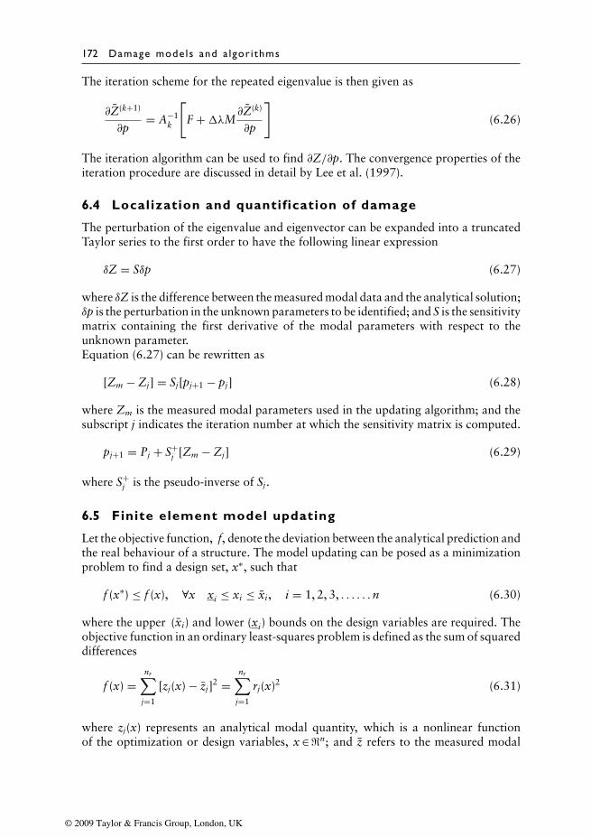
172 Damage mode ls and a lgor i thms
The iteration scheme for the repeated eigenvalue is then given as
∂Z(k+1)
∂p= A−1
k
[F +�λM∂Z
(k)
∂p
](6.26)
The iteration algorithm can be used to find ∂Z/∂p. The convergence properties of theiteration procedure are discussed in detail by Lee et al. (1997).
6.4 Localization and quantification of damage
The perturbation of the eigenvalue and eigenvector can be expanded into a truncatedTaylor series to the first order to have the following linear expression
δZ = Sδp (6.27)
where δZ is the difference between the measured modal data and the analytical solution;δp is the perturbation in the unknown parameters to be identified; and S is the sensitivitymatrix containing the first derivative of the modal parameters with respect to theunknown parameter.Equation (6.27) can be rewritten as
[Zm − Zj] = Sj[pj+1 − pj] (6.28)
where Zm is the measured modal parameters used in the updating algorithm; and thesubscript j indicates the iteration number at which the sensitivity matrix is computed.
pj+1 = Pj + S+j [Zm − Zj] (6.29)
where S+j is the pseudo-inverse of Sj.
6.5 Finite element model updating
Let the objective function, f, denote the deviation between the analytical prediction andthe real behaviour of a structure. The model updating can be posed as a minimizationproblem to find a design set, x∗, such that
f (x∗) ≤ f (x), ∀x xi ≤ xi ≤ xi, i = 1, 2, 3, . . . . . .n (6.30)
where the upper (xi) and lower (xi) bounds on the design variables are required. Theobjective function in an ordinary least-squares problem is defined as the sum of squareddifferences
f (x) =nr∑
j=1
[zj(x) − zj]2 =nr∑
j=1
rj(x)2 (6.31)
where zj(x) represents an analytical modal quantity, which is a nonlinear functionof the optimization or design variables, x ∈ �n; and z refers to the measured modal
© 2009 Taylor & Francis Group, London, UK
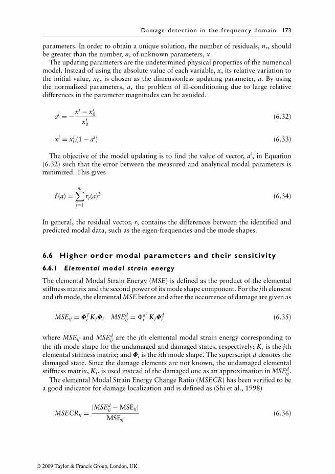
Damage detect ion in the frequency domain 173
parameters. In order to obtain a unique solution, the number of residuals, nr, shouldbe greater than the number, n, of unknown parameters, x.
The updating parameters are the undetermined physical properties of the numericalmodel. Instead of using the absolute value of each variable, x, its relative variation tothe initial value, x0, is chosen as the dimensionless updating parameter, a. By usingthe normalized parameters, a, the problem of ill-conditioning due to large relativedifferences in the parameter magnitudes can be avoided.
ai = −xi − xi0
xi0
(6.32)
xi = xi0(1 − ai) (6.33)
The objective of the model updating is to find the value of vector, ai, in Equation(6.32) such that the error between the measured and analytical modal parameters isminimized. This gives
f (a) =nr∑
j=1
rj(a)2 (6.34)
In general, the residual vector, r, contains the differences between the identified andpredicted modal data, such as the eigen-frequencies and the mode shapes.
6.6 Higher order modal parameters and their sensitivity
6.6.1 Elemental modal strain energy
The elemental Modal Strain Energy (MSE) is defined as the product of the elementalstiffness matrix and the second power of its mode shape component. For the jth elementand ith mode, the elemental MSE before and after the occurrence of damage are given as
MSEij = ΦTi K jΦi MSEd
ij = �dT
i K jΦdi (6.35)
where MSEij and MSEdij are the jth elemental modal strain energy corresponding to
the ith mode shape for the undamaged and damaged states, respectively; K j is the jthelemental stiffness matrix; and Φi is the ith mode shape. The superscript d denotes thedamaged state. Since the damage elements are not known, the undamaged elementalstiffness matrix, K j, is used instead of the damaged one as an approximation in MSEd
ij.The elemental Modal Strain Energy Change Ratio (MSECR) has been verified to be
a good indicator for damage localization and is defined as (Shi et al., 1998)
MSECRij = |MSEdij − MSEij|MSEij
(6.36)
© 2009 Taylor & Francis Group, London, UK
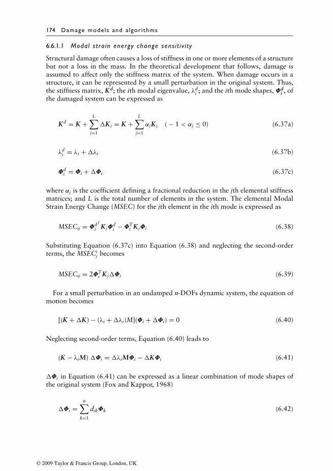
174 Damage mode ls and a lgor i thms
6.6.1.1 Modal s t ra in energy change sens i t i v i t y
Structural damage often causes a loss of stiffness in one or more elements of a structurebut not a loss in the mass. In the theoretical development that follows, damage isassumed to affect only the stiffness matrix of the system. When damage occurs in astructure, it can be represented by a small perturbation in the original system. Thus,the stiffness matrix, Kd; the ith modal eigenvalue, λd
i ; and the ith mode shapes, Φdi , of
the damaged system can be expressed as
Kd = K +L∑
j=1
�K j = K +L∑
j=1
αjK j ( − 1 < αj ≤ 0) (6.37a)
λdi = λi +�λi (6.37b)
Φdi = Φi +�Φi (6.37c)
where αj is the coefficient defining a fractional reduction in the jth elemental stiffnessmatrices; and L is the total number of elements in the system. The elemental ModalStrain Energy Change (MSEC) for the jth element in the ith mode is expressed as
MSECij = ΦdT
i K jΦdi − ΦT
i K jΦi (6.38)
Substituting Equation (6.37c) into Equation (6.38) and neglecting the second-orderterms, the MSECi
j becomes
MSECij = 2ΦTi K j�Φi (6.39)
For a small perturbation in an undamped n-DOFs dynamic system, the equation ofmotion becomes
[(K +�K) − (λi +�λi)M](Φi +�Φi) = 0 (6.40)
Neglecting second-order terms, Equation (6.40) leads to
(K − λiM) �Φi = �λiMΦi −�KΦi (6.41)
�Φi in Equation (6.41) can be expressed as a linear combination of mode shapes ofthe original system (Fox and Kappor, 1968)
�Φi =n∑
k=1
dikΦk (6.42)
© 2009 Taylor & Francis Group, London, UK
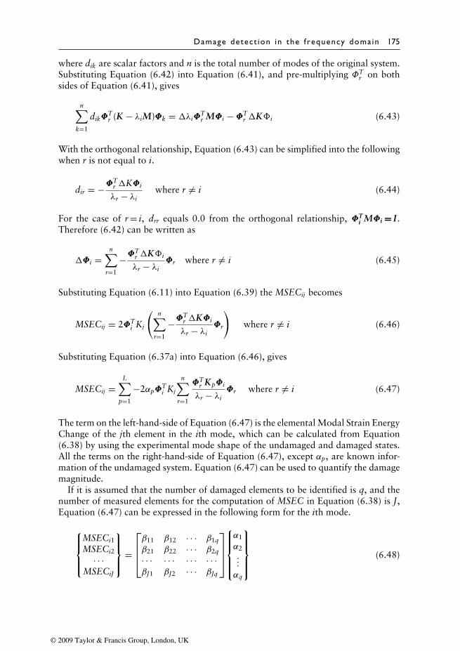
Damage detect ion in the frequency domain 175
where dik are scalar factors and n is the total number of modes of the original system.Substituting Equation (6.42) into Equation (6.41), and pre-multiplying ΦT
r on bothsides of Equation (6.41), gives
n∑k=1
dikΦTr (K − λiM)Φk = �λiΦ
Tr MΦi − ΦT
r �K�i (6.43)
With the orthogonal relationship, Equation (6.43) can be simplified into the followingwhen r is not equal to i.
dir = −ΦTr �KΦi
λr − λiwhere r = i (6.44)
For the case of r = i, drr equals 0.0 from the orthogonal relationship, ΦTi MΦi = I .
Therefore (6.42) can be written as
�Φi =n∑
r=1
−ΦTr �K�i
λr − λiΦr where r = i (6.45)
Substituting Equation (6.11) into Equation (6.39) the MSECij becomes
MSECij = 2ΦTi Kj
(n∑
r=1
−ΦTr �KΦi
λr − λiΦr
)where r = i (6.46)
Substituting Equation (6.37a) into Equation (6.46), gives
MSECij =L∑
p=1
−2αpΦTi Kj
n∑r=1
ΦTr KpΦi
λr − λiΦr where r = i (6.47)
The term on the left-hand-side of Equation (6.47) is the elemental Modal Strain EnergyChange of the jth element in the ith mode, which can be calculated from Equation(6.38) by using the experimental mode shape of the undamaged and damaged states.All the terms on the right-hand-side of Equation (6.47), except αp, are known infor-mation of the undamaged system. Equation (6.47) can be used to quantify the damagemagnitude.
If it is assumed that the number of damaged elements to be identified is q, and thenumber of measured elements for the computation of MSEC in Equation (6.38) is J,Equation (6.47) can be expressed in the following form for the ith mode.
MSECi1
MSECi2
· · ·MSECiJ
=
β11 β12 · · · β1q
β21 β22 · · · β2q
· · · · · · · · · · · ·βJ1 βJ2 · · · βJq
α1
α2...
αq
(6.48)
© 2009 Taylor & Francis Group, London, UK
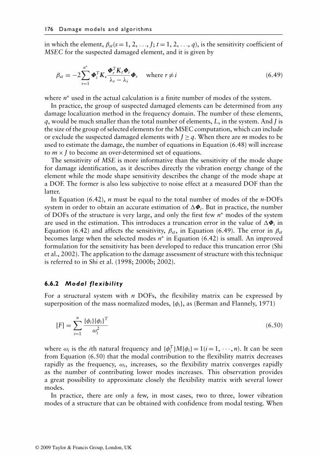
176 Damage mode ls and a lgor i thms
in which the element, βst(s = 1, 2, . . ., J; t = 1, 2, . . ., q), is the sensitivity coefficient ofMSEC for the suspected damaged element, and it is given by
βst = −2n∗∑
r=1
ΦTi K s
ΦTr K tΦi
λr − λiΦr where r = i (6.49)
where n∗ used in the actual calculation is a finite number of modes of the system.In practice, the group of suspected damaged elements can be determined from any
damage localization method in the frequency domain. The number of these elements,q, would be much smaller than the total number of elements, L, in the system. And J isthe size of the group of selected elements for the MSEC computation, which can includeor exclude the suspected damaged elements with J ≥ q. When there are m modes to beused to estimate the damage, the number of equations in Equation (6.48) will increaseto m × J to become an over-determined set of equations.
The sensitivity of MSE is more informative than the sensitivity of the mode shapefor damage identification, as it describes directly the vibration energy change of theelement while the mode shape sensitivity describes the change of the mode shape ata DOF. The former is also less subjective to noise effect at a measured DOF than thelatter.
In Equation (6.42), n must be equal to the total number of modes of the n-DOFssystem in order to obtain an accurate estimation of �Φi. But in practice, the numberof DOFs of the structure is very large, and only the first few n∗ modes of the systemare used in the estimation. This introduces a truncation error in the value of �Φi inEquation (6.42) and affects the sensitivity, βst, in Equation (6.49). The error in βst
becomes large when the selected modes n∗ in Equation (6.42) is small. An improvedformulation for the sensitivity has been developed to reduce this truncation error (Shiet al., 2002). The application to the damage assessment of structure with this techniqueis referred to in Shi et al. (1998; 2000b; 2002).
6.6.2 Modal f lexibi l i ty
For a structural system with n DOFs, the flexibility matrix can be expressed bysuperposition of the mass normalized modes, {φi}, as (Berman and Flannely, 1971)
[F] =n∑
i=1
{φi}{φi}T
ω2i
(6.50)
where ωi is the ith natural frequency and {φTi }M{φi} = 1(i = 1, · · · , n). It can be seen
from Equation (6.50) that the modal contribution to the flexibility matrix decreasesrapidly as the frequency, ωi, increases, so the flexibility matrix converges rapidlyas the number of contributing lower modes increases. This observation providesa great possibility to approximate closely the flexibility matrix with several lowermodes.
In practice, there are only a few, in most cases, two to three, lower vibrationmodes of a structure that can be obtained with confidence from modal testing. When
© 2009 Taylor & Francis Group, London, UK
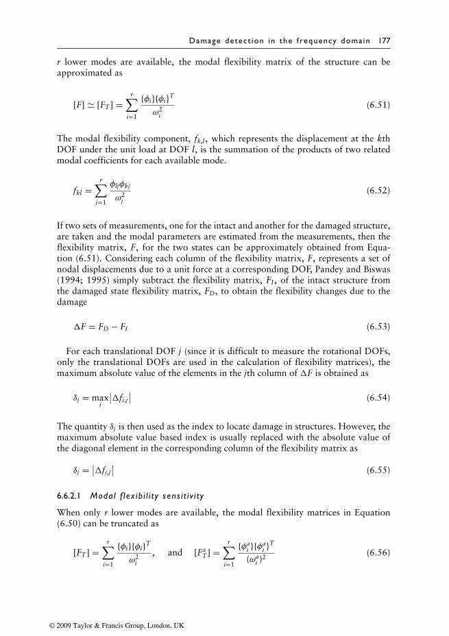
Damage detect ion in the frequency domain 177
r lower modes are available, the modal flexibility matrix of the structure can beapproximated as
[F] � [FT ] =r∑
i=1
{φi}{φi}T
ω2i
(6.51)
The modal flexibility component, fk,l, which represents the displacement at the kthDOF under the unit load at DOF l, is the summation of the products of two relatedmodal coefficients for each available mode.
fkl =r∑
j=1
φljφkj
ω2j
(6.52)
If two sets of measurements, one for the intact and another for the damaged structure,are taken and the modal parameters are estimated from the measurements, then theflexibility matrix, F, for the two states can be approximately obtained from Equa-tion (6.51). Considering each column of the flexibility matrix, F, represents a set ofnodal displacements due to a unit force at a corresponding DOF, Pandey and Biswas(1994; 1995) simply subtract the flexibility matrix, FI, of the intact structure fromthe damaged state flexibility matrix, FD, to obtain the flexibility changes due to thedamage
�F = FD − FI (6.53)
For each translational DOF j (since it is difficult to measure the rotational DOFs,only the translational DOFs are used in the calculation of flexibility matrices), themaximum absolute value of the elements in the jth column of �F is obtained as
δj = maxi
∣∣�fi,j∣∣ (6.54)
The quantity δj is then used as the index to locate damage in structures. However, themaximum absolute value based index is usually replaced with the absolute value ofthe diagonal element in the corresponding column of the flexibility matrix as
δj = ∣∣�fj,j∣∣ (6.55)
6.6.2.1 Modal f lex ib i l i t y sens i t i v i t y
When only r lower modes are available, the modal flexibility matrices in Equation(6.50) can be truncated as
[FT ] =r∑
i=1
{φi}{φi}T
ω2i
, and [FaT ] =
r∑i=1
{φai }{φa
i }T
(ωai )2
(6.56)
© 2009 Taylor & Francis Group, London, UK
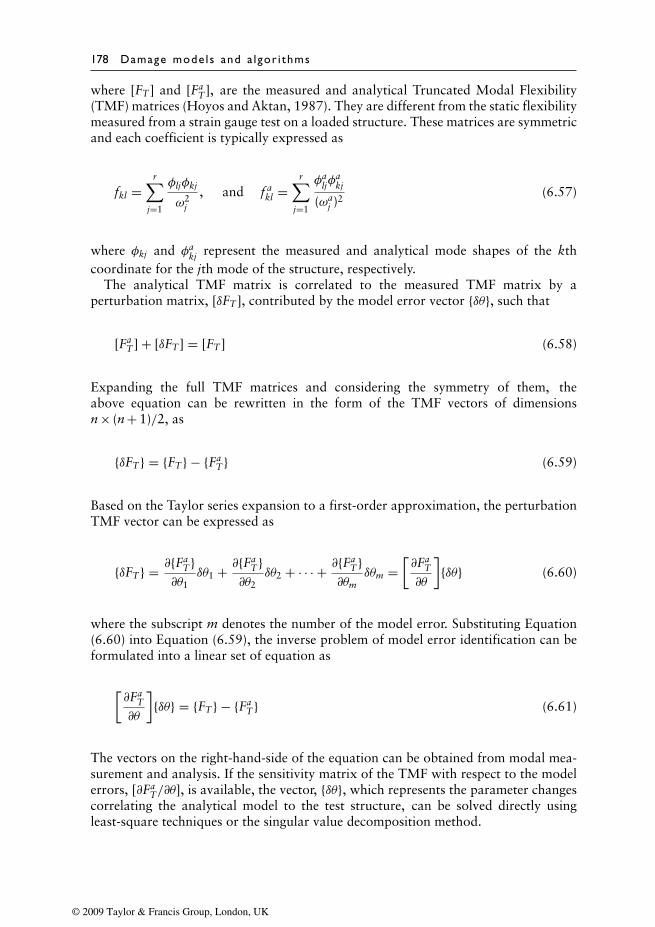
178 Damage mode ls and a lgor i thms
where [FT ] and [FaT ], are the measured and analytical Truncated Modal Flexibility
(TMF) matrices (Hoyos and Aktan, 1987). They are different from the static flexibilitymeasured from a strain gauge test on a loaded structure. These matrices are symmetricand each coefficient is typically expressed as
fkl =r∑
j=1
φljφkj
ω2j
, and f akl =
r∑j=1
φaljφ
akj
(ωaj )2
(6.57)
where φkj and φakj represent the measured and analytical mode shapes of the kth
coordinate for the jth mode of the structure, respectively.The analytical TMF matrix is correlated to the measured TMF matrix by a
perturbation matrix, [δFT ], contributed by the model error vector {δθ}, such that
[FaT ] + [δFT ] = [FT ] (6.58)
Expanding the full TMF matrices and considering the symmetry of them, theabove equation can be rewritten in the form of the TMF vectors of dimensionsn × (n + 1)/2, as
{δFT} = {FT} − {FaT} (6.59)
Based on the Taylor series expansion to a first-order approximation, the perturbationTMF vector can be expressed as
{δFT} = ∂{FaT}∂θ1
δθ1 + ∂{FaT}∂θ2
δθ2 + · · · + ∂{FaT}
∂θmδθm =
[∂Fa
T
∂θ
]{δθ} (6.60)
where the subscript m denotes the number of the model error. Substituting Equation(6.60) into Equation (6.59), the inverse problem of model error identification can beformulated into a linear set of equation as
[∂Fa
T
∂θ
]{δθ} = {FT} − {Fa
T} (6.61)
The vectors on the right-hand-side of the equation can be obtained from modal mea-surement and analysis. If the sensitivity matrix of the TMF with respect to the modelerrors, [∂Fa
T/∂θ], is available, the vector, {δθ}, which represents the parameter changescorrelating the analytical model to the test structure, can be solved directly usingleast-square techniques or the singular value decomposition method.
© 2009 Taylor & Francis Group, London, UK
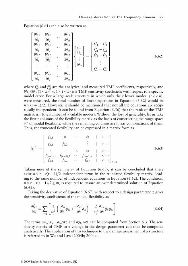
Damage detect ion in the frequency domain 179
Equation (6.61) can also be written as
∂f11
∂θ1
∂f11
∂θ2· · · ∂f11
∂θm∂f21
∂θ1
∂f21
∂θ2· · · ∂f21
∂θm∂f22
∂θ1
∂f22
∂θ2· · · ∂f22
∂θm...
......
...
∂fnn
∂θ1
∂fnn
∂θ2· · · ∂fnn
∂θm
δθ1δθ2...
δθm
=
f x11 − f a
11
f x21 − f a
21
f x22 − f a
22
...
f xnn − f a
nn
(6.62)
where f akl and f x
kl are the analytical and measured TMF coefficients, respectively, and∂fkl/∂θi, (1 ≤ k ≤ n, 1 ≤ l ≤ k) is a TMF sensitivity coefficient with respect to a specificmodel error. For a large-scale structure in which only the r lower modes, (r<< n),were measured, the total number of linear equations in Equation (6.62) would ben × (n + 1)/2. However, it should be mentioned that not all the equations are recip-rocally independent. It can be found from Equation (6.56) that the rank of the TMFmatrix is r (the number of available modes). Without the lost of generality, let us takethe first r columns of the flexibility matrix as the basis of constructing the range space�n of modal flexibility, while the remaining columns are linear combinations of them.Thus, the truncated flexibility can be expressed in a matrix form as
[FT ] =
f1,1 ⊗ · · · ⊗ | × · · ·f2,1 f2,2
... | × · · ·...
.... . . ⊗ | × · · ·
f(n−1),1 f(n−1),2 · · · f(n−1),r | × · · ·fn,1 fn,2 · · · fn,r | × · · ·
n×n
(6.63)
Taking note of the symmetry of Equation (6.63), it can be concluded that thereexist n × r − r(r − 1)/2 independent terms in the truncated flexibility matrix, lead-ing to the same number of independent equations in Equation (6.62). The condition,n × r − r(r − 1)/2 ≥ m, is required to ensure an over-determined solution of Equation(6.62).
Taking the derivative of Equation (6.57) with respect to a design parameter θi givesthe sensitivity coefficients of the modal flexibility as
∂fkl
∂θi=
r∑j=1
[1
ω2j
(∂φlj
∂θiφkj + ∂φkj
∂θiφlj
)− 2
ω3j
∂ωj
∂θiφljφkj
](6.64)
The terms ∂ωj/∂θi, ∂φlj/∂θi and ∂φkj/∂θi can be computed from Section 6.3. The sen-sitivity matrix of TMF to a change in the design parameter can then be computedanalytically. The application of this technique to the damage assessment of a structureis referred to in Wu and Law (2004b; 2004c).
© 2009 Taylor & Francis Group, London, UK
180 Damage mode ls and a lgor i thms
6.6.3 Unit load surface
The modal flexibility matrix of a linear structural system is given in Equation (6.51),while the modal flexibility relating two modal coefficients is given in Equation (6.52).The modal deflection at point k under uniform unit load all over the structure can beapproximated as
u(k) =n∑
l=1
fk,l =m∑
r=1
φr(k)∑n
l=1 φr(l)ω2
r(6.65)
The Uniform Load Surface (ULS) is defined as the deflection vector of the structureunder uniform load (Zhang and Aktan, 1998)
UT = {u(k)} = FT · L (6.66)
where L = {1, · · · , 1}T1×n is the unit vector representing the uniform load acting on
the structure. From Equations (6.52) and (6.65), Zhang and Aktan (1998) observedtwo features of the ULS comparative to the modal flexibility. Firstly, the ULS is lesssensitive to measurement noise than the modal flexibility, because the summation ofall the modal coefficients of the corresponding mode,
∑nl=1 φr(l) in Equation (6.65),
averages out the random error at each measuring point. The second feature is that theULS converges more rapidly with the lower modes than the modal flexibility. This isalso because of the summation of all the modal coefficients of each mode to the ULSin Equation (6.65). Since the modal coefficients of higher modes tend to cancel eachother more than those of the lower modes, the lower modes tend to contribute morethan the higher modes to the ULS coefficients. This cancelling effect does not existwith the modal flexibility formulation in Equation (6.52). These special propertiesmake the ULS a potentially stable and sensitive damage indicator for structural healthmonitoring.
6.7 The curvatures
For a continuous structure without damage, the mode shape curvature has a smoothcurve shape along the span of the structure. When there is a fault, a change in thecurvature in the form of a peak or abrupt slope, appears near the fault position. Thislocal peak position in the curvature can be used as an index to locate local damage instructures. The most practical advantage of the method is that the curvature computa-tion does not refer to the parameters of the intact structure as a baseline. It is also moresensitive to closely distributed damages than the method using mode shape changes. Ithas been concluded (Pandey et al., 1991; Lu et al., 2002) that the curvature techniqueis the most efficient to locate these changes in the smooth curves based on the studyof damage detection with mode shapes and flexibility for beam-like structures. Thefollowing sections describe the finite difference approach, which is commonly adoptedfor the computation of the curvature from the mode shape. The more sophisticatedapproach of using polynomial approximation is also given. The gap-smoothing tech-nique is also discussed for the case of incomplete measurement. These techniques areapplicable not only to the mode shape information but also to the flexibility and unitload surface as described in last section.
© 2009 Taylor & Francis Group, London, UK
Damage detect ion in the frequency domain 181
6.7.1 Mode shape curvature
An alternative to using mode shapes to obtain spatial information about vibrationchanges is using mode shape derivatives, such as curvature. The curvature val-ues are computed from the displacement mode shape using the central differenceapproximation for mode i and DOF j as
φ′′j,i = φj−1,i − 2φj,i + φj+1,i
�l2(6.67)
where �l is the distance between the two DOFs considered.
6.7.2 Modal f lexibi l i ty curvature
Once the flexibility matrix of a structure is estimated from the measured modal param-eters, the flexibility curvature can be approximated by a finite difference scheme. Inthe damage localization of a simply supported reinforced concrete beam (Lu et al.,2002), the flexibility curvature is obtained as
fci = fi−1,i−1 − 2fi,i + fi+1,i+1
�l2(6.68)
where fi,i and �l are the ith diagonal element of the flexibility matrix and the distancebetween the two DOFs considered, respectively; and fci is the ith item in the flexibilitycurvature vector.
6.7.3 Unit load surface curvature
Starting from this section, the focus will be on damage detection with plate-like struc-tures. It is assumed that the dynamic response of the plate is acquired by placing sensorsin a rectangular grid, such that the mode shapes and the ULS can further be estimated.
An existing curvature-based damage detection technique computes the curvaturesusing a finite central differentiation procedure. When this technique is incorporatedwith two-dimensional ULS, the curvatures of the ULS are calculated by a Laplacianoperator in each normal direction along the sensor grid as
uxx(xi, yj) = u(xi+1, yj) − 2u(xi, yj) + u(xi−1, yj)h2
x(6.69a)
uyy(xi, yj) = u(xi, yj+1) − 2u(xi, yj) + u(xi, yj−1)h2
y(6.69b)
in which the ULS is grouped from a vector into a matrix according to the coordinatesof measuring points in the grid, and the grid is assumed to be equally spaced in the x-and y-directions, as shown in Figure 6.1. hx and hy are the uniform grid spacings inthe corresponding directions.
If two sets of measurements, one from the intact structure and another from thedamaged structure, are taken and the modal parameters are estimated from the mea-surements, the ULS curvature at point (xi, yj) for the two states can be obtained using
© 2009 Taylor & Francis Group, London, UK

182 Damage mode ls and a lgor i thms
u(xi�1, yj�1)
u(xi�1, yj�1) u(xi�1, yj�1)
u(xi�1, yj�1)
u(xi, yj�1)
u(xi, yj�1)
u(xi�1, yj) u(xi�1, yj)
u(xi, yj)
Figure 6.1 Gapped grid for curve fitting at measuring point (xi,yj)
Equations (6.52) and (6.69). The presence of the irregularity in the damaged curvaturecan be detected by subtracting the ULS curvature of the intact state from the curvatureof the damaged state. Thereby a map of the damage index can be formulated as
d(xi, yj) = [αxx| uDxx(xi, yj) − uxx(xi, yj)| + αyy| uD
yy(xi, yj) − uyy(xi, yj)|]2(6.70)
where |•| denotes the absolute value; uxx and uyy are the measured ULS curvaturevalues of the intact structure at the corresponding point in the x- and y-directions,respectively, uD
xx and uDyy are those of the suspected damaged structure; and αxx and
αyy are the weights that can be set from 0.0 to 1.0 to consider the importance of thecurvature in the corresponding directions.
If the structure is undamaged when the second set of measurement is carried out, thedifference between the two sets of measured ULS curvature would be due to measure-ment noise only. Therefore values of the damage index map, d(xi, yj), slightly oscillatearound zero without any distinct peak. In contrast, if the structure is damaged, peaksor slopes will clearly show up at the damaged zone of the plate, as shown later in thenumerical study in Section 6.7.6.
6.7.4 Chebyshev polynomial approximation
The accuracy of the central difference method is well known depending on the densityof the measurement grid. If the ULS values are estimated on a sparse grid, it will inducea very large error in calculating the curvature from differentiation. The followingChebyshev polynomial in two variables is adopted to model the ULS distribution toavoid this error (Wu and Law, 2004a):
u(x, y) =N∑
i=1
M∑j=1
cijTi(x)Tj(y) (6.71)
where Ti(x) and Tj(y) are the first kind Chebyshev polynomials, and N and M aretheir orders. To map the standard Chebyshev polynomials from the plane domain of
© 2009 Taylor & Francis Group, London, UK
Damage detect ion in the frequency domain 183
{ξ,µ} = [−1, 1] × [−1, 1] to the physical plate domain of {x, y} = [0, Lx] × [0, Ly], twolinear transfer functions are defined
ξ = 2x/Lx − 1, µ = 2y/Ly − 1 (6.72)
Lx and Ly are the dimensions of the plate in the x- and y-directions, respectively. TheChebyshev polynomials of variable x is then written as
T1(x) = 1√π
, T2(x) =√
2π
(2xLx
− 1)
,
Ti+1(x) = 2(
2xLx
− 1)
Ti(x) − Ti−1(x), i = 2, 3, · · · , N − 1 (6.73)
The polynomials of variable y can be formulated similarly.Without loss of generality, it is assumed that P = N × M measuring points are set on
the rectangular sensor grid so that the ULS can be estimated at these points. Equation(6.71) will be satisfied at all the measuring points, and the Chebyshev polynomialapproximation can be written in a matrix form
{u(xi, yj)}P×1 = [T(xi)T(yj)]P×P{cij}P×1 (6.74)
The coefficient vector, {cij}, can then be solved as
{cij}P×1 = [T(xi)T(yj)]−1P×P{u(xi, yj)}P×1 (6.75)
or obtained by the least-squares method if the number of measuring points Q>P.
{cij}P×1 = ([T(xi)T(yj)]TQ×P[T(xi)T(yj)]Q×P)−1
[T(xi)T(yj)]TQ×P{u(xi, yj)}Q×1 (6.76)
It is a better choice to have the measuring points at the Chebyshev zeros ( xi, yj), which
ensure the convergence for any continuous function that satisfies a Dini–Lipschitzcondition (Mason and Handscomb, 2003). The location of these N × M zeros isgiven by
xi =(
cos(i − 0.5)π
N+ 1
)Lx
2, i = 1, · · · , N (6.77a)
yj =(
cos(j − 0.5)π
M+ 1
)Ly
2, j = 1, · · · , M (6.77b)
© 2009 Taylor & Francis Group, London, UK
184 Damage mode ls and a lgor i thms
The corresponding coefficients can be explicitly obtained as
cij = λP
N∑r=1
M∑s=1
u( xi, yj) cos
(i(r − 0.5)π
N
)cos
(j(s − 0.5)π
M
),
{i = 1, · · · , N; j = 1, · · · , Mr = 1, · · · , N; s = 1, · · · , M
}(6.78)
where
λ =
1 for i = 1, j = 12 for i = 1, j = 1 or i = 1, j = 14 for i = 1, j = 1
By making use of the orthogonal property of the Chebyshev polynomial, the curvatureof the ULS can then be approximated by the second derivatives of the Chebyshevpolynomials in Equation (6.71) as
uxx(x, y) =N∑
i=1
M∑j=1
cij∂T2
i (x)∂x2
Tj(y), uyy(x, y) =N∑
i=1
M∑j=1
cijTi(x)∂T2
j (y)
∂y2(6.79a)
and
uxy(x, y) =N∑
i=1
M∑j=1
cij∂Ti(x)∂x
∂Tj(y)∂y
(6.79b)
Therefore, the formulation of the damage index in Equation (6.70) can be rewritten as
d(xi, yj) = [αxx|uDxx − uxx| + αyy| uD
yy − uyy| + αxy|uDxy − uxy|]2
(6.80)
It should be noted that the discussions in Sections 6.7.4 and 6.7.5 for a two-dimensionaldistribution of ULS curvature are applicable for the mode shape curvature andflexibility curvature obtained from the same set of measured mode shape information.
6.7.5 The gap-smoothing technique
Most damage-index methods require the ‘footprint’, or baseline data set, of the intactstructure for comparison, to inspect the change in modal parameters due to dam-age. Typically the ‘footprint’ is obtained either from measurements of the undamagedstructure, or from a finite element model of the intact structure. An inaccurate finiteelement model can introduce large model errors, and degrade or even lead to incorrectresults in the damage detection. However, most suspected damaged civil structureswere constructed several decades ago, and the ‘footprint’ of the structures in the intactstate is not available. To avoid this difficulty, Ratcliffe and Bagaria (1998) proposedthe ‘gapped-smoothing’ technique with modal curvature, which allows for damagedetection in a beam structure without prior knowledge of the undamaged state. The
© 2009 Taylor & Francis Group, London, UK
Damage detect ion in the frequency domain 185
‘gapped-smoothing’ technique has now been extended and applied to bi-dimensionalULS curvature for the plate structures.
The basic idea of the method is that the ULS curvature of the plate, without anydamage, has a smooth surface, and it can be approximated by a cubic polynomial intwo variables:
u(x, y) = c0 + c1x + c2y + c3x2 + c4y2 + c5xy + c6x2y + c7xy2 (6.81)
where the coefficients, ci, can be evaluated by a curve-fitting process on the estimatedULS curvature of the damaged structure on a gapped grid of measuring points asshown in Figure 6.1. Particularly, to obtain the smoothed ULS curvature at point(xi, yj), curvature data at all the adjacent points, but not the point (xi, yj) itself, areused to evaluate the coefficients, ci. This process is repeated for each measuring point togive a smooth ULS curvature to model the undamaged plate structure. The presence ofthe peak in the ULS curvature due to local damage can then be detected by subtractingthe smoothed curvature from the estimated curvature of the damaged structure. Thedamage index map is given similar to Equation (6.80) as
d(xi, yj) = [αxx|uDxx − uxx| + αyy|uD
yy − uyy| + αxy|uDxy − uxy|]2
(6.82)
6.7.5.1 The un i form load sur face curvature sens i t i v i t y
Consider a damaged plate divided into ne rectangular elements. The characteristicequation for this undamped structural dynamic system can be expressed as
K{φ}r − ω2r M{φ}r = 0 (6.83)
It is assumed that any occurrence of structural damage only causes a reduction in localstiffness, while the mass matrix remains unchanged. The stiffness and mass matricesof the damaged plate are expressed as
K = K0 +�K =ne∑
e=1
peke, M = M0 (6.84)
in which ke is the element stiffness matrix of the intact plate and pe indicates the healthstatus of the corresponding element, where pe = 1 stands for the intact and pe< 1 forthe damaged state. M0 and M are the mass matrices of the damaged and intact states.
Taking the derivative of Equation (6.83) with respect to the stiffness parameter, pe,and noting the relations in Equation (6.84), gives
(K − ω2
r M) ∂{φ}r
∂pe=(
2ωr∂ω
∂piM − ke
){φ}r (6.85)
The sensitivity of the natural frequency and mode shapes with respect to the parameter,pe, can be calculated using Nelson’s method (Nelson, 1976).
© 2009 Taylor & Francis Group, London, UK
186 Damage mode ls and a lgor i thms
To find the sensitivity of the ULS curvature ∂uc(x, y)/∂pe, the sensitivity of the ULSat the measuring points needs to be calculated first. Taking the derivative of Equation(6.65) with respect to the parameter, pe, gives
∂u(xi, yj)∂pe
= ∂uk
∂pe=
m∑r=1
n∑l=1
[1ω2
r
(∂φkr
∂peφlr + ∂φlr
∂peφkr
)− 2ω3
r
∂ωr
∂pkφkrφlr
](6.86)
Substituting the sensitivities of the mode shape and the modal frequency in Equation(6.15) into Equation (6.86), the ULS sensitivities on the sensor grids are obtained.Further, taking the derivative of Equation (6.76) with respect to the parameter, pe, andsubstituting Equation (6.86), the sensitivity of the Chebyshev coefficients is obtained as{
∂cij
∂pe
}P×1
=([T(xi)T(yj)]T
Q×P[T(xi)T(yj)]Q×P
)−1[T(xi)T(yj)]T
Q×P
{∂u(xi, yj)∂pe
}Q×1
(6.87)
If the measuring points are located at the Chebyshev zeros ( xi, yj), substituting Equation
(6.86) into Equation (6.78) also gives the sensitivity of Chebyshev coefficients as
∂cij
∂pk= λ
P
N∑r=1
M∑s=1
∂u( xi, yj)
∂pkcos
(i(r − 0.5)π
N
)cos
(j(s − 0.5)π
M
),
{i = 1, · · · , Nj = 1, · · · , M
(6.88)
Finally the sensitivity of the ULS curvature with respect to the stiffness parameter, pe,can be derived from the Equation (6.79) and calculated as
∂ucxx(x, y)∂pe
=N∑
i=1
M∑j=1
∂cij
∂pe
∂T2i (x)∂x2
Tj(y),∂ucyy(x, y)∂pe
=N∑
i=1
M∑j=1
∂cij
∂peTi(x)
∂T2j (y)
∂y2
(6.89a)
and
∂ucxy(x, y)∂pe
=N∑
i=1
M∑j=1
∂cij
∂pe
∂Ti(x)∂x
∂Tj(y)∂y
(6.89b)
Since the structural damage is assumed as a reduction of local stiffness in Equa-tion (6.84), the changes in the ULS curvature caused by damage can be expandedwith the first-order Taylor series approximation.
�ucxx(xi, yj) = ucDxx − ucxx = ∂ucxx
∂p1�p1 + ∂ucxx
∂p2�p2 + · · · + ∂ucxx
∂pne�pne (6.90)
in which ne indicates the number of suspected damaged elements. Similar relations canbe obtained for the curvature changes �ucyy(xi, yj) and �ucxy(xi, yj).
© 2009 Taylor & Francis Group, London, UK
Damage detect ion in the frequency domain 187
Applying Equation (6.90) to all the measuring points and rearranging in matrixform, gives
∂ucxx(x1, y1)∂p1
∂ucxx(x1, y1)∂p2
· · · ∂ucxx(x1, y1)∂pne
......
......
∂ucxx(xN , yM)∂p1
∂ucxx(xN , yM)∂p2
· · · ∂ucxx(xN , yM)∂pne
......
......
∂ucyy(xN , yM)∂p1
∂ucyy(xN , yM)∂p2
· · · ∂ucyy(xN , yM)∂pne
......
......
∂ucxy(xN , yM)∂p1
∂ucxy(xN , yM)∂p2
· · · ∂ucxy(xN , yM)∂pne
�p1
�p2...
�pne
=
ucDxx(x1, y1) − ucxx(x1, y1)
...
ucDxx(xN , yM) − ucxx(xN , yM)
...
ucDyy(xN , yM) − ucyy(xN , yM)
...
ucDxy(xN , yM) − ucxy(xN , yM)
(6.91)
or
S · {�pe} = {�uc} (6.92)
It should be noted that Equation (6.91) comprises ne unknown variables and a totalof neq = 3 × Q linear equations. To ensure that a unique over-determined solution canbe found, the condition neq ≥ ne is required. The Singular Value Decomposition (SVD)with error-truncation technique (Wu and Law, 2005a) is adopted to solve the linearizedequations. To reflect the nonlinear effects from large magnitude damage or interactionbetween the variables, the equations are solved by an iterative algorithm as follows.
Step 1. Initialize the vector of stiffness parameter as {pe|nee=1}0 = 1.
Step 2. At the beginning of each iteration, construct the ULS curvature sensitivitymatrix, Si, for the ith iteration, and calculate the curvature change, {�uc}i,due to damage.
Step 3. Solve the increment of parameter vector as, {�pe}i = S∗i {�uc}i, where S∗
i isthe generalized inverse of Si from the SVD technique.
Step 4. Normalize the increment vector, {�pe}i = {�pe}i ×α, so that the conditionβmin ≤�pe|ne
e=1 ≤βpos is satisfied. α is a scale factor and βmin and βpos are theconvergence limits as shown below.
© 2009 Taylor & Francis Group, London, UK
188 Damage mode ls and a lgor i thms
Step 5. Evaluate the new stiffness parameter vector as{
pe∣∣ne
e=1
}i= {
pe∣∣ne
e=1
}i−1
·(1 + {�pe}i). If ε1 = |{�pe}|< ε1 or ε2 = |{�uc}i+1|
|{�uc}i | < ε2, the solution is consid-
ered converged at{
pe∣∣ne
e=1
}i. Otherwise, go to Step 2 and repeat the process
until the condition is satisfied.
The scale factor, α, in Step 4 is calculated as α= min(
βminmin (�pe|ne
e=1), βpos
max (�pe|nee=1)
), in
which the range [βmin,βpos] is set to compromise the convergence speed and solutionstability. A wider range could speed up the solution convergence, but for some cases,it may lead to a divergent solution, while a narrower range would have the oppositeeffect. The application of this technique in the damage assessment of a plate structureis referred to in Wu and Law (2005a).
6.7.6 Numerical examples of damage local ization
Two plates with different boundary conditions, namely a four-side simply supportedplate and a cantilever plate, are used as examples to demonstrate how the changein the ULS curvature can be used as an index to locate damage in a plate. Theseexamples were chosen because each of them exhibits a different behaviour with theload distribution. For example, in a uniformly loaded four-side simply supported plate,both the maximum bending moment and flexural displacement occur at the geometricalcentre of the plate, where flexural damage would most likely occur. In the cantileverplate, the maximum bending moment and shear force occur at the clamped edge wherethe flexural displacement is a minimum, so that the damage is usually in the form of acrack along the fixed edge.
The configuration of the cantilever plate is shown in Figure 6.2. The dimensions ofthe plate are 600 mm × 480 mm with a thickness of 20 mm. The finite element model ofthe plate consists of 15 × 12 = 180 equal size square Reissner–Mindlin plate elements.Three DOFs, which are translational along the Z-axis and rotational along the X- andY-axes, are used at each node. The simply supported plate has the same dimensionsand finite element mesh as the cantilever plate, but with different boundary conditions.
It is assumed that damage will affect only the stiffness matrix of a structure. Thechange in the stiffness matrix due to damage is modelled by a reduction in the elasticmodulus of the corresponding element. The extent of damage is then linearly relatedto the degree of reduction in the elastic modulus, E.
For each damage case, the natural frequencies and corresponding mode shapes areobtained from the finite element analysis. The ULS curvatures are calculated sepa-rately using Equations (6.69) and (6.79). Since the three DOFs at each node in theReissner–Mindlin plate elements are uncoupled, one can choose whether to calculatethe translational DOF-based ULS curvature or rotational DOF-based ULS curvature.Results from the simulation study show that the latter is more sensitive to local damageand less sensitive to random noise than the former. However, since there it is difficultto measure the rotational DOFs with current dynamic testing techniques, only thetranslational DOFs along the Z-axis are used in the study. Equations (6.70), (6.80)and (6.82) are then used separately in the calculation of the damage index based onchanges in the ULS curvature and the gapped-smoothing technique. The weights αxx,αyy and αxy are all taken equal to unity. The effectiveness of the methods from the
© 2009 Taylor & Francis Group, London, UK
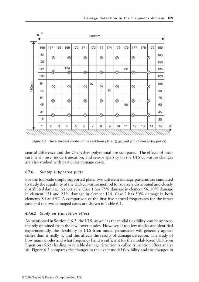
Damage detect ion in the frequency domain 189
166 167 168 169
124
97
84
131
56
...
...
170 171 172
600mm48
0mm
173 174 175 176 177 178 179 180
15 X
Y
1 2 3 4 5 6 7 8 9 10 11 12 13 14
16
31
46
61
76
91
106
121
136
151
30
45
60
75
90
105
120
135
150
165
Figure 6.2 Finite element model of the cantilever plate (⊗ gapped grid of measuring points)
central difference and the Chebyshev polynomial are compared. The effects of mea-surement noise, mode truncation, and sensor sparsity on the ULS curvature changesare also studied with particular damage cases.
6.7.6.1 S imply supported p late
For the four-side simply supported plate, two different damage patterns are simulatedto study the capability of the ULS curvature method for sparsely distributed and closelydistributed damage, respectively. Case 1 has 75% damage in element 56, 50% damagein element 131 and 25% damage in element 124. Case 2 has 50% damage in bothelements 84 and 97. A comparison of the first five natural frequencies for the intactcase and the two damaged cases are shown in Table 6.1.
6.7.6.2 Study on truncat ion ef fec t
As mentioned in Section 6.6.2, the ULS, as well as the modal flexibility, can be approx-imately obtained from the few lower modes. However, if too few modes are identifiedexperimentally, the flexibility or ULS from modal parameters will generally appearstiffer than it really is, and this affects the results of damage detection. The study ofhow many modes and what frequency band is sufficient for the modal-based ULS fromEquation (6.52) leading to reliable damage detection is called truncation effect analy-sis. Figure 6.3 compares the changes in the exact modal flexibility and the changes in
© 2009 Taylor & Francis Group, London, UK
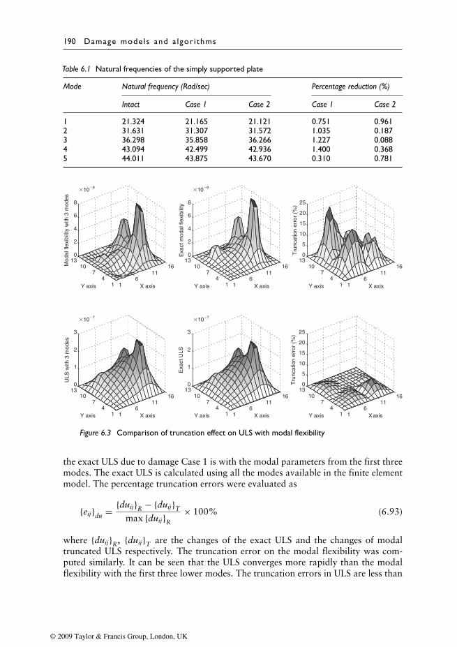
190 Damage mode ls and a lgor i thms
Table 6.1 Natural frequencies of the simply supported plate
Mode Natural frequency (Rad/sec) Percentage reduction (%)
Intact Case 1 Case 2 Case 1 Case 2
1 21.324 21.165 21.121 0.751 0.9612 31.631 31.307 31.572 1.035 0.1873 36.298 35.858 36.266 1.227 0.0884 43.094 42.499 42.936 1.400 0.3685 44.011 43.875 43.670 0.310 0.781
16
1116
14
710
130
2
4
6
8
�10�9
X axisY axis
Mod
al fl
exib
ility
with
3 m
odes
16
1116
14
710
130
1
2
3
�10�7
X axisY axis
ULS
with
3 m
odes
16
1116
14
710
130
2
4
6
8
�10�9
X axisY axis
Exa
ct m
odal
flex
ibili
ty
16
1116
14
710
130
1
2
3
�10�7
X axisY axis
Exa
ct U
LS
16
1116
14
710
130
5
10
15
20
25
X axisY axis
Tru
ncat
ion
erro
r (%
)
16
1116
14
710
130
5
10
15
20
25
X axisY axis
Tru
ncat
ion
erro
r (%
)
Figure 6.3 Comparison of truncation effect on ULS with modal flexibility
the exact ULS due to damage Case 1 is with the modal parameters from the first threemodes. The exact ULS is calculated using all the modes available in the finite elementmodel. The percentage truncation errors were evaluated as
{eij}du = {duij}R − {duij}T
max {duij}R
× 100% (6.93)
where {duij}R, {duij}T are the changes of the exact ULS and the changes of modaltruncated ULS respectively. The truncation error on the modal flexibility was com-puted similarly. It can be seen that the ULS converges more rapidly than the modalflexibility with the first three lower modes. The truncation errors in ULS are less than
© 2009 Taylor & Francis Group, London, UK
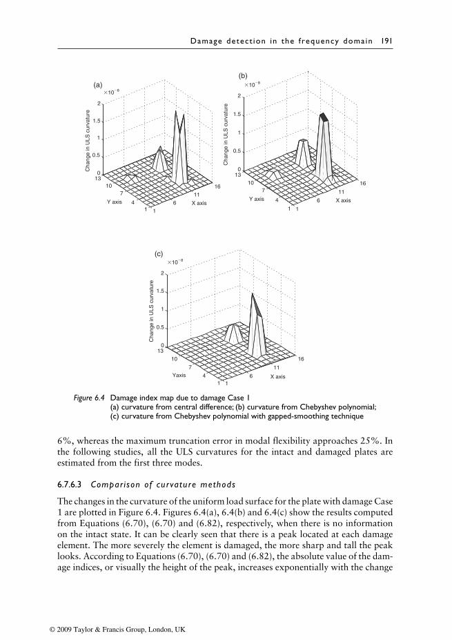
Damage detect ion in the frequency domain 191
16
11
16
14
7
10
130
0.5
1
1.5
2
�10�8
X axisYaxis
Cha
nge
in U
LS c
urva
ture
1
6
11
16
1
4
710
130
0.5
1
1.5
2
�10�8
X axisY axis
Cha
nge
in U
LS c
urva
ture
1
6
11
16
14
710
130
0.5
1
1.5
2
�10�8
X axisY axis
Cha
nge
in U
LS c
urva
ture
(a)
(b)
(c)
Figure 6.4 Damage index map due to damage Case 1(a) curvature from central difference; (b) curvature from Chebyshev polynomial;(c) curvature from Chebyshev polynomial with gapped-smoothing technique
6%, whereas the maximum truncation error in modal flexibility approaches 25%. Inthe following studies, all the ULS curvatures for the intact and damaged plates areestimated from the first three modes.
6.7.6.3 Compar i son of curvature methods
The changes in the curvature of the uniform load surface for the plate with damage Case1 are plotted in Figure 6.4. Figures 6.4(a), 6.4(b) and 6.4(c) show the results computedfrom Equations (6.70), (6.70) and (6.82), respectively, when there is no informationon the intact state. It can be clearly seen that there is a peak located at each damageelement. The more severely the element is damaged, the more sharp and tall the peaklooks. According to Equations (6.70), (6.70) and (6.82), the absolute value of the dam-age indices, or visually the height of the peak, increases exponentially with the change
© 2009 Taylor & Francis Group, London, UK
192 Damage mode ls and a lgor i thms
in ULS curvature, and the 25% damage in element 124 shows only a very tiny peakcompared with the 75% damage in element 56. Nevertheless, it does not mean the dam-age with 25% stiffness reduction is the limit the methods can detect. For this case, boththe central difference method (Figure 6.4(a)) and the Chebyshev polynomial method(Figure 6.4(b)) can successfully locate all three damaged elements, whereas, when priorknowledge of the intact structure is not available, the Chebyshev polynomial methodwith gapped-smoothing technique failed to locate the damage in element 124.
6.7.6.4 Reso lut ion of damage loca l izat ion
It is well known that most damage-index methods can localize the spatially distributeddamage quite accurately, but have difficulty detecting contiguous multiple damages.Damage Case 2 is specially simulated to study the effectiveness of the ULS curvaturemethod for closely distributed damages. Figure 6.5 shows the results of damage detec-tion for this case. It can be seen that the two damaged elements 84 and 97 are locatedclose together at the centre of the plate, and they can be separately detected by inspect-ing the change in the ULS curvature, computed either from central difference or by theChebyshev polynomial. However, when given the modal data for the damaged stateonly, although the damaged region can be localized from Figure 6.5(c), it is hard totell exactly which element is damaged.
6.7.6.5 Cant i lever p late
It is always a difficult problem for damage index methods to reliably identify dam-age near the supported boundary. For a one-side clamped slab, it is intuitive that thedamage is more likely to develop near and along the fixed edge where the maximumbending moment occurs. Two typical damage cases for the cantilevered slab are simu-lated. Case 3 has 75% damage in element 15, 50% damage in elements 13 and 14 and25% damage in element 12. Case 4 has 75% damage in element 8, 50% damage inelements 7 and 9 and 25% damage in elements 6 and 10. The damage in Case 3 startsfrom one end of the fixed edge and continues along the edge across four elements. Thedamage in Case 4 models a band of damage symmetrically located in the middle andalong the fixed edge across five elements. The natural frequencies for the intact anddamaged structures are listed in Table 6.2.
The results of damage detection for damage Cases 3 and 4 are shown in Figures 6.6and 6.7, respectively. It can be seen from Figure 6.6 that the damage band near theboundary can be detected by inspecting the ULS change calculated by both methods,even without the initial curvature of intact structure. The ULS curvature by Chebyshevpolynomial method gives relatively better localization of the damage than those fromcentral difference with a parabolic curve surface compared with a sharp change fromcentral difference method with more than one peak, while the damage location cannotbe exactly validated when the intact structure curvature is absent. A similar observationcan be obtained from Figure 6.7.
6.7.6.6 Ef fec t o f sensor spars i t y
In a real experiment, it is not practical to have a very fine sensor mesh to measurethe dynamic response of all the nodes in the finite element model. To study the effect
© 2009 Taylor & Francis Group, London, UK
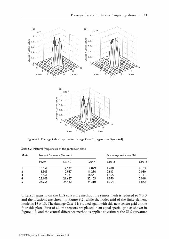
Damage detect ion in the frequency domain 193
1
6
11
16
1
4
7
10
130
0.2
0.4
0.6
0.8
1
�10�8
X axisY axis
Cha
nge
in U
LS c
urva
ture
16
11
16
14
710
130
0.2
0.4
0.6
0.8
1
�10�8
X axisY axis
Cha
nge
in U
LS c
urva
ture
1
6
11
16
1
4
7
1013
0
0.2
0.4
0.6
0.8
1
(a) (b)
(c)
�10�8
X axisY axis
Cha
nge
in U
LS c
urva
ture
Figure 6.5 Damage index map due to damage Case 2 (Legends as Figure 6.4)
Table 6.2 Natural frequencies of the cantilever plate
Mode Natural frequency (Rad/sec) Percentage reduction (%)
Intact Case 3 Case 4 Case 3 Case 4
1 8.051 7.932 7.879 1.478 2.1832 11.305 10.987 11.296 2.813 0.0803 16.561 16.32 16.541 1.455 0.1214 22.109 21.667 22.105 1.999 0.0185 24.765 24.442 24.310 1.304 1.872
of sensor sparsity on the ULS curvature method, the sensor mesh is reduced to 7 × 5and the locations are shown in Figure 6.2, while the nodes grid of the finite elementmodel is 16 × 13. The damage Case 1 is studied again with this new sensor grid on thefour-side plate. First of all, the sensors are placed in an equal spatial grid as shown inFigure 6.2, and the central difference method is applied to estimate the ULS curvature
© 2009 Taylor & Francis Group, London, UK
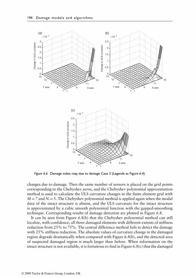
194 Damage mode ls and a lgor i thms
1
6
11
16
1
4
7
10130
0.5
1
1.5
2
2.5
�10�6
X axisY axis
Cha
nge
in U
LS c
urva
ture
1
6
11
16
1
4
7
10130
0.5
1
1.5
2
2.5
�10�6
X axisY axis
Cha
nge
in U
LS c
urva
ture
1
6
11
16
14
7
10130
0.5
1
1.5
2
2.5
3
(a) (b)
(c)
�10�6
X axisY axis
Cha
nge
in U
LS c
urva
ture
Figure 6.6 Damage index map due to damage Case 3 (Legends as Figure 6.4)
changes due to damage. Then the same number of sensors is placed on the grid pointscorresponding to the Chebyshev zeros, and the Chebyshev polynomial approximationmethod is used to calculate the ULS curvature changes in the finite element grid withM = 7 and N = 5. The Chebyshev polynomial method is applied again when the modaldata of the intact structure is absent, and the ULS curvature for the intact structureis approximated by a cubic smooth polynomial function with the gapped-smoothingtechnique. Corresponding results of damage detection are plotted in Figure 6.8.
It can be seen from Figure 6.8(b) that the Chebyshev polynomial method can stilllocalize, with confidence, all three damaged elements with different extents of stiffnessreduction from 25% to 75%. The central difference method fails to detect the damagewith 25% stiffness reduction. The absolute values of curvature change in the damagedregion degrade dramatically when compared with Figure 6.4(b), and the detected areaof suspected damaged region is much larger than before. When information on theintact structure is not available, it is fortuitous to find in Figure 6.8(c) that the damaged
© 2009 Taylor & Francis Group, London, UK
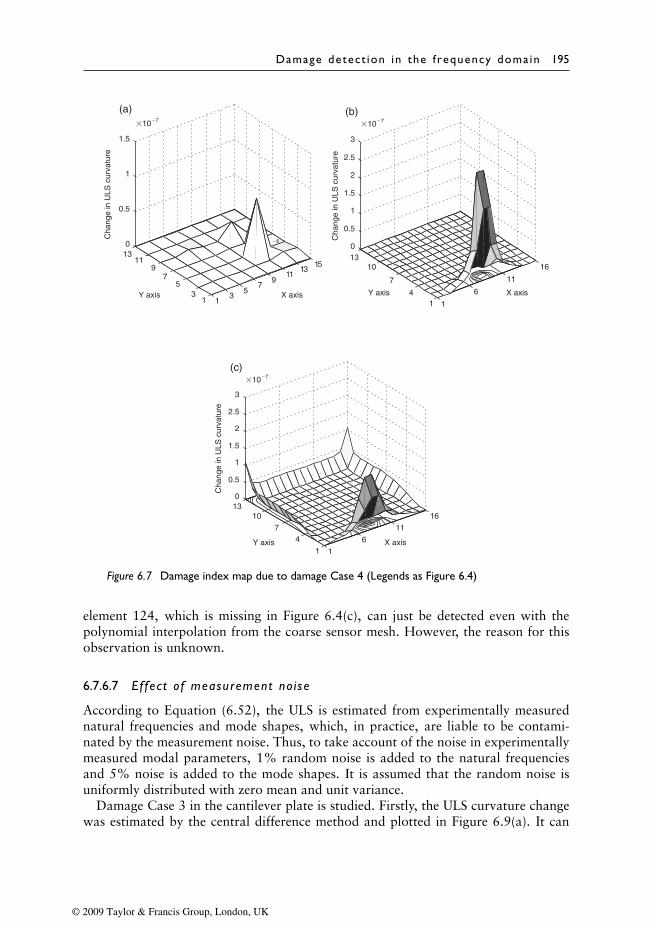
Damage detect ion in the frequency domain 195
1
6
11
16
1
47
10130
0.5
1
1.5
2
2.5
3
�10�7
X axisY axis
Cha
nge
in U
LS c
urva
ture
1
6
11
16
14
7
10130
0.5
1
1.5
2
2.5
3
�10�7
X axisY axis
Cha
nge
in U
LS c
urva
ture
13
57
911
1315
13
57
911
130
0.5
1
1.5
�10�7
X axisY axis
Cha
nge
in U
LS c
urva
ture
(a) (b)
(c)
�6
Figure 6.7 Damage index map due to damage Case 4 (Legends as Figure 6.4)
element 124, which is missing in Figure 6.4(c), can just be detected even with thepolynomial interpolation from the coarse sensor mesh. However, the reason for thisobservation is unknown.
6.7.6.7 Ef fec t o f measurement no i se
According to Equation (6.52), the ULS is estimated from experimentally measurednatural frequencies and mode shapes, which, in practice, are liable to be contami-nated by the measurement noise. Thus, to take account of the noise in experimentallymeasured modal parameters, 1% random noise is added to the natural frequenciesand 5% noise is added to the mode shapes. It is assumed that the random noise isuniformly distributed with zero mean and unit variance.
Damage Case 3 in the cantilever plate is studied. Firstly, the ULS curvature changewas estimated by the central difference method and plotted in Figure 6.9(a). It can
© 2009 Taylor & Francis Group, London, UK
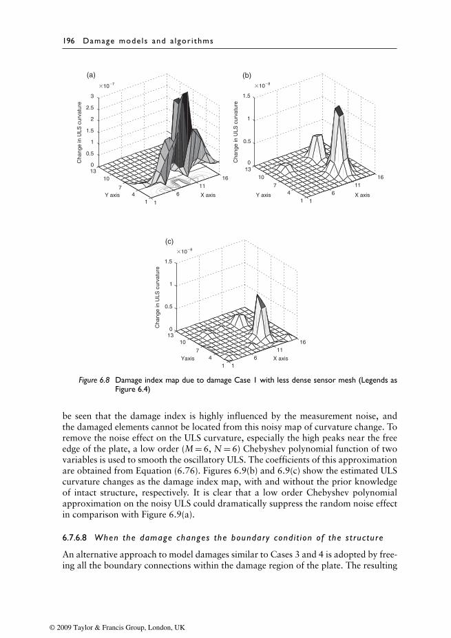
196 Damage mode ls and a lgor i thms
16
1116
1
47
10130
0.5
1
1.5
�10�8
X axisYaxis
Cha
nge
in U
LS c
urva
ture
16
1116
1
47
10130
0.5
1
1.5
�10�8
X axisY axis
Cha
nge
in U
LS c
urva
ture
1
6
11
16
14
7
10130
0.5
1
1.5
2
2.5
3
�10�7
X axisY axis
Cha
nge
in U
LS c
urva
ture
(a)
(c)
(b)
Figure 6.8 Damage index map due to damage Case 1 with less dense sensor mesh (Legends asFigure 6.4)
be seen that the damage index is highly influenced by the measurement noise, andthe damaged elements cannot be located from this noisy map of curvature change. Toremove the noise effect on the ULS curvature, especially the high peaks near the freeedge of the plate, a low order (M = 6, N = 6) Chebyshev polynomial function of twovariables is used to smooth the oscillatory ULS. The coefficients of this approximationare obtained from Equation (6.76). Figures 6.9(b) and 6.9(c) show the estimated ULScurvature changes as the damage index map, with and without the prior knowledgeof intact structure, respectively. It is clear that a low order Chebyshev polynomialapproximation on the noisy ULS could dramatically suppress the random noise effectin comparison with Figure 6.9(a).
6.7.6.8 When the damage changes the boundary cond i t ion of the s t ructure
An alternative approach to model damages similar to Cases 3 and 4 is adopted by free-ing all the boundary connections within the damage region of the plate. The resulting
© 2009 Taylor & Francis Group, London, UK
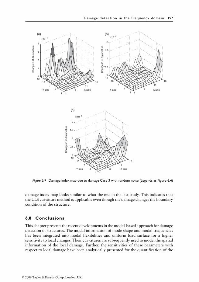
Damage detect ion in the frequency domain 197
1
6
11
16
1
4
7
10130
0.5
1
1.5
2
�10�6
X axisY axis
Cha
nge
in U
LS c
urva
ture
1
6
11
16
1
4
7
10130
0.5
1
1.5
2
�10�6
X axisY axis
Cha
nge
in U
LS c
urva
ture
1
6
11
16
1
4
7
10130
2
4
6
8
�10�6
X axisY axis
Cha
nge
in U
LS c
urva
ture
(a) (b)
(c)
Figure 6.9 Damage index map due to damage Case 3 with random noise (Legends as Figure 6.4)
damage index map looks similar to what the one in the last study. This indicates thatthe ULS curvature method is applicable even though the damage changes the boundarycondition of the structure.
6.8 Conclusions
This chapter presents the recent developments in the modal-based approach for damagedetection of structures. The modal information of mode shape and modal frequencieshas been integrated into modal flexibilities and uniform load surface for a highersensitivity to local changes. Their curvatures are subsequently used to model the spatialinformation of the local damage. Further, the sensitivities of these parameters withrespect to local damage have been analytically presented for the quantification of the
© 2009 Taylor & Francis Group, London, UK

198 Damage mode ls and a lgor i thms
local changes. All the above have helped to answer the questions: Does any damageoccur? Where does it occur? and what is the amplitude? Other questions such as:what type of damage it is? will need the inclusion of different types of damage modelsdescribed in Chapter 3 to provide the answer.
These modal-based methods have the disadvantage of limited measured informationand may not be applicable to large civil structures with thousands of DOFs. Othertypes of approaches are sought to provide more measured information economicallyand they are discussed in Chapters 7 and 8.
© 2009 Taylor & Francis Group, London, UK
Chapter 7
System identification basedon response sensitivity
7.1 Time-domain methods
System identification can also be conducted with information directly from the timeresponse. The time-domain approach has an advantage over the frequency-domainmethod in that there is an unlimited supply of measured information. Moreover, thedamping properties of structures cannot be readily estimated in the frequency-domainmethod. Another advantage is that there is no requirement for complete measurementsin space and state. However, the detrimental effect from measurement noise (Hjelm-stad and Banan, 1995) remains significant with time-domain methods (Ge and Soong,1998). This chapter addresses the system identification approach based on the sen-sitivity of the measured response with respect to a system parameter. Features of theapproach with different applications are presented.
7.2 The response sensitivity
For a general finite element model of a linear elastic time-invariant structure, theequation of motion is given by
[M]{x} + [C]{x} + [K]{x} = [B]{F} (7.1)
where [M], [C] and [K] are the system mass, damping and stiffness matrices, respec-tively. Rayleigh damping is adopted, which is of the form [C] = a1[M] + a2[K], wherea1 and a2 are constants to be determined from two modal damping ratios; {x}, {x} and{x} are the acceleration, velocity and displacement response vectors of the structure;{F} is a vector of applied forces with matrix [B] mapping these forces to the associateddegrees-of-freedom (DOFs) of the structure. The dynamic responses of the structurescan be obtained by direct numerical integration using the Newmark method.
7.2.1 The computational approach
For the perturbation of a system parameter, �α, the perturbed equation of motionis obtained by differentiating both sides of Equation (7.1) with respect to the system
© 2009 Taylor & Francis Group, London, UK

200 Damage mode ls and a lgor i thms
parameter. Assuming the parameter is related only to the stiffness of the dynamicsystem, the following is obtained
[M]{∂x∂αi
}+[C]
{∂x∂αi
}+[K]
{∂x∂αi
}= −∂[K]
∂αi{x}−a2
∂[K]∂αi
{x}(i = 1, 2, . . .N)(7.2a)
where {∂x/∂αi }, {∂x/∂αi } and {∂x/∂αi } are vectors of the displacement, velocity andacceleration sensitivities with respect to the unknown parameter; and αi is the param-eter in the ith element or other stiffness parameter of the system. A similar equationcan be written for the perturbation of parameters which are related to the system massand damping matrices.
Let Y = ∂x∂αi
, Y = ∂x∂αi
andY = ∂x∂αi
,
thus,
[M]{Y} + [C]{Y} + [K]{Y} = −∂[K]∂αi
{x} − a2∂[K]∂αi
{x} (7.2b)
Since {x} and {x} have been obtained from Equation (7.1), the right-hand-side ofEquation (7.2b) can be considered as an equivalent forcing function, and the equationis of the same form as Equation (7.1). Therefore, the sensitivities Y, Y and Y can alsobe obtained using the Newmark method.
7.2.2 The analyt ical formulation
Equation (7.1) may be rewritten in the state-space formulation as
X = K∗X + F (7.3)
where X =[
xx
]2n×1
, K∗ =[
0 I−M−1K −M−1C
]2n×2n
, F =[
0M−1[B]F
]2n×1
and X represents a vector of state variables with a length 2n containing the displace-ments and velocities of the nodes. These differential equations are then converted todiscrete equations using exponential matrix representation
Xk+1 = AXk + DFk (7.4)
A = eK∗h, D = K∗−1(A − I)
where A is the exponential matrix and (k + 1) denotes the value at the (k + 1)th timestep of computation. The time step h represents the time increment between the variablestates Xk and Xk+1 in the computation. I is a unit matrix. The dynamic response ofthe system can be obtained from Equation (7.4) with zero initial conditions. Once thedisplacement and velocity responses are obtained, the acceleration response can beobtained by directly differentiating the velocity response.
The first differential of the dynamic response with respect to a physical parameterof the system, αi, can be obtained by differentiating both sides of Equation (7.3) with
© 2009 Taylor & Francis Group, London, UK
System ident i f i ca t ion based on response sens i t i v i ty 201
respect to parameter αi of an element as
∂X∂αi
= K∗ ∂X∂αi
+ ∂K∗
∂αiX
= K∗ ∂X∂αi
+ 0
−M−1 ∂K∂αi
x
+ 0
−a2M−1 ∂K∂αi
x
(i = 1, 2, . . .N) (7.5)
It is noted that the system mass matrix is not dependent on the physical parameter,αi, and thus the partial derivative ∂M/∂αi in Equation (7.5) vanishes. Let Y = ∂X/∂αi,where Y is the vector of displacement and velocity differentials with respect toparameter αi in the time domain.
Put P = 0
−M−1 ∂K∂αi
x
and G = 0
−a2M−1 ∂K∂αi
x
Equation (7.5) can then be rewritten as
Y = K∗Y +[P + G
](7.6)
It is noted that Equation (7.6) has the same form as Equation (7.3). The displacementand velocity response sensitivities can then be obtained in a discretized form similar toEquation (7.4) as,
Yk+1 = AYk + D[Pk + Gk] (7.7)
and the acceleration response sensitivity can be obtained by direct differentiating thevelocity sensitivity.
7.2.3 Main features of the response sensit iv ity
The main features of the response sensitivity have been studied (Lu and Law, 2007a)with an example of a plane frame structure to study the sensitivities generated for dif-ferent types of excitation. The frame structure consists of eleven Euler–Bernoulli beamelements with twelve nodes each with three DOFs as shown in Figure 7.1. The frame isfixed at nodes 1 and 12, modelled with large translational and rotational stiffnesses of1.5 × 1010 kN/m and 1.5 × 10⁹ kN-m/rad, respectively. The mass density of the mate-rial is 2.7 × 10³ kg/m3 and the elastic modulus of the material is 69 × 109 N/m2. Theheight and width of the frame are 1.2 m and 0.6 m, respectively, and the cross-sectionaldimensions of the member are b = 0.01 m and h0 = 0.02 m with the second moment ofinertia in the plane of bending equal to 6.67 × 10⁻⁹ m4. The first five undamped naturalfrequencies of the intact frame are 13.095, 57.308, 76.697, 152.410 and 196.485 Hz.The Rayleigh damping model is adopted with the damping ratios of the first two modestaken equal to 0.01. The equivalent Rayleigh coefficients a1 and a2 are 1.3395 and4.52 × 10−5, respectively.
Sinusoidal, impulsive and random excitations are applied separately at node 2 in thex-direction to generate the dynamic responses and their sensitivities with respect to a
© 2009 Taylor & Francis Group, London, UK
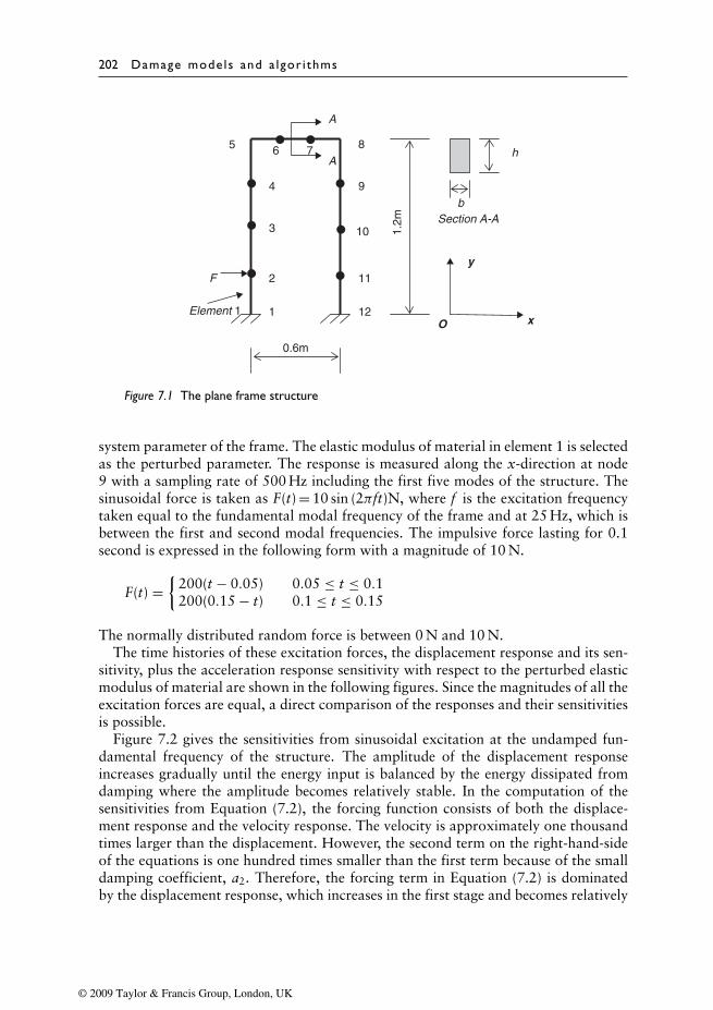
202 Damage mode ls and a lgor i thms
A
1
2
3
4
6 75 8
9
10
11
12
A
b
h
1.2m Section A-A
x
y
O
F
Element 1
0.6m
Figure 7.1 The plane frame structure
system parameter of the frame. The elastic modulus of material in element 1 is selectedas the perturbed parameter. The response is measured along the x-direction at node9 with a sampling rate of 500 Hz including the first five modes of the structure. Thesinusoidal force is taken as F(t) = 10 sin (2πft)N, where f is the excitation frequencytaken equal to the fundamental modal frequency of the frame and at 25 Hz, which isbetween the first and second modal frequencies. The impulsive force lasting for 0.1second is expressed in the following form with a magnitude of 10 N.
F(t) ={
200(t − 0.05) 0.05 ≤ t ≤ 0.1200(0.15 − t) 0.1 ≤ t ≤ 0.15
The normally distributed random force is between 0 N and 10 N.The time histories of these excitation forces, the displacement response and its sen-
sitivity, plus the acceleration response sensitivity with respect to the perturbed elasticmodulus of material are shown in the following figures. Since the magnitudes of all theexcitation forces are equal, a direct comparison of the responses and their sensitivitiesis possible.
Figure 7.2 gives the sensitivities from sinusoidal excitation at the undamped fun-damental frequency of the structure. The amplitude of the displacement responseincreases gradually until the energy input is balanced by the energy dissipated fromdamping where the amplitude becomes relatively stable. In the computation of thesensitivities from Equation (7.2), the forcing function consists of both the displace-ment response and the velocity response. The velocity is approximately one thousandtimes larger than the displacement. However, the second term on the right-hand-sideof the equations is one hundred times smaller than the first term because of the smalldamping coefficient, a2. Therefore, the forcing term in Equation (7.2) is dominatedby the displacement response, which increases in the first stage and becomes relatively
© 2009 Taylor & Francis Group, London, UK
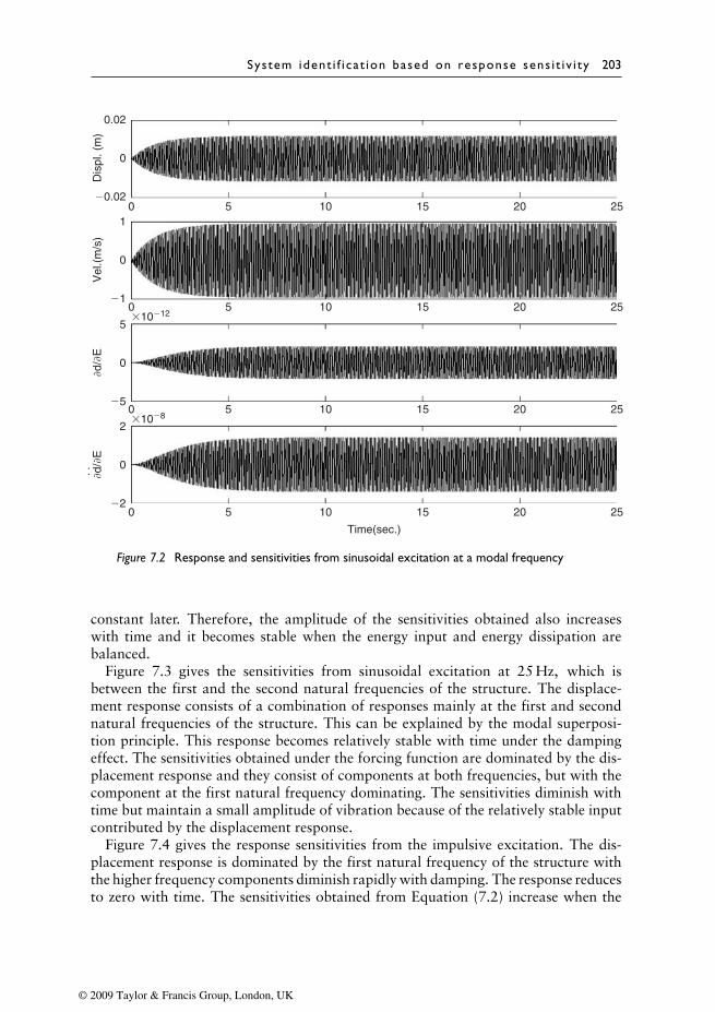
System ident i f i ca t ion based on response sens i t i v i ty 203
2
�2
0
0 5 10 15 2520
Time(sec.)
�d/
�E
5
�5
0
�d/
�E
1
�1
0
Vel
.(m
/s)
0.02
�0.02
0
Dis
pl. (
m)
0�10�8
�10�12
5 10 15 2520
0 5 10 15 2520
0 5 10 15 2520
Figure 7.2 Response and sensitivities from sinusoidal excitation at a modal frequency
constant later. Therefore, the amplitude of the sensitivities obtained also increaseswith time and it becomes stable when the energy input and energy dissipation arebalanced.
Figure 7.3 gives the sensitivities from sinusoidal excitation at 25 Hz, which isbetween the first and the second natural frequencies of the structure. The displace-ment response consists of a combination of responses mainly at the first and secondnatural frequencies of the structure. This can be explained by the modal superposi-tion principle. This response becomes relatively stable with time under the dampingeffect. The sensitivities obtained under the forcing function are dominated by the dis-placement response and they consist of components at both frequencies, but with thecomponent at the first natural frequency dominating. The sensitivities diminish withtime but maintain a small amplitude of vibration because of the relatively stable inputcontributed by the displacement response.
Figure 7.4 gives the response sensitivities from the impulsive excitation. The dis-placement response is dominated by the first natural frequency of the structure withthe higher frequency components diminish rapidly with damping. The response reducesto zero with time. The sensitivities obtained from Equation (7.2) increase when the
© 2009 Taylor & Francis Group, London, UK
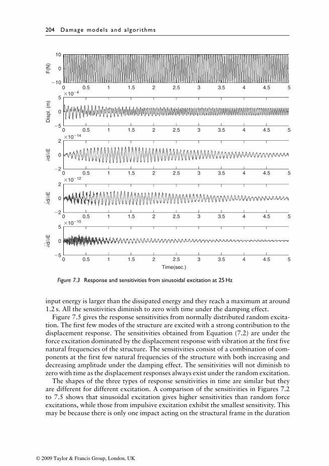
204 Damage mode ls and a lgor i thms
5
�5
0
0 0.5 1 1.5 2 2.5 3 3.5 54 4.5
0 0.5 1 1.5 2 2.5 3 3.5 54 4.5
0 0.5 1 1.5 2 2.5 3 3.5 54 4.5
0 0.5 1 1.5 2 2.5 3 3.5 54 4.5
0 0.5 1 1.5 2 2.5 3 3.5 54 4.5
Time(sec.)
�d/
�E
2
�2
0
�d/
�E
2
�2
0
�d/
�E
5
�5
0
10
�10
0
Dis
pl. (
m)
F(N
)
�10�10
�10�12
�10�14
�10�4
Figure 7.3 Response and sensitivities from sinusoidal excitation at 25 Hz
input energy is larger than the dissipated energy and they reach a maximum at around1.2 s. All the sensitivities diminish to zero with time under the damping effect.
Figure 7.5 gives the response sensitivities from normally distributed random excita-tion. The first few modes of the structure are excited with a strong contribution to thedisplacement response. The sensitivities obtained from Equation (7.2) are under theforce excitation dominated by the displacement response with vibration at the first fivenatural frequencies of the structure. The sensitivities consist of a combination of com-ponents at the first few natural frequencies of the structure with both increasing anddecreasing amplitude under the damping effect. The sensitivities will not diminish tozero with time as the displacement responses always exist under the random excitation.
The shapes of the three types of response sensitivities in time are similar but theyare different for different excitation. A comparison of the sensitivities in Figures 7.2to 7.5 shows that sinusoidal excitation gives higher sensitivities than random forceexcitations, while those from impulsive excitation exhibit the smallest sensitivity. Thismay be because there is only one impact acting on the structural frame in the duration
© 2009 Taylor & Francis Group, London, UK
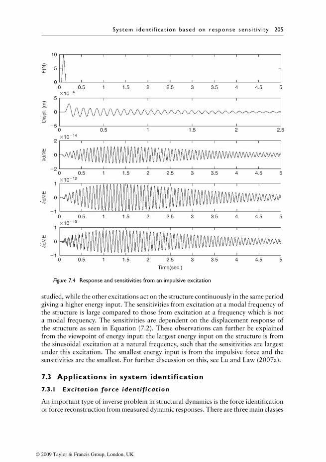
System ident i f i ca t ion based on response sens i t i v i ty 205
1
�1
0
0 0.5 1 1.5 2 2.5 3 3.5 54 4.5
0 0.5 1 1.5 2 2.5 3 3.5 54 4.5
0 0.5 1 1.5 2 2.5 3 3.5 54 4.5
0 0.5 1 1.5 2 2.5
0 0.5 1 1.5 2 2.5 3 3.5 54 4.5
Time(sec.)
�d/
�E
1
�1
0
�d/
�E
2
�2
0
�d/
�E
5
�5
0
10
0
5
Dis
pl. (
m)
F(N
)
�10�10
�10�12
�10�14
�10�4
Figure 7.4 Response and sensitivities from an impulsive excitation
studied, while the other excitations act on the structure continuously in the same periodgiving a higher energy input. The sensitivities from excitation at a modal frequency ofthe structure is large compared to those from excitation at a frequency which is nota modal frequency. The sensitivities are dependent on the displacement response ofthe structure as seen in Equation (7.2). These observations can further be explainedfrom the viewpoint of energy input: the largest energy input on the structure is fromthe sinusoidal excitation at a natural frequency, such that the sensitivities are largestunder this excitation. The smallest energy input is from the impulsive force and thesensitivities are the smallest. For further discussion on this, see Lu and Law (2007a).
7.3 Applications in system identification
7.3.1 Excitation force identif ication
An important type of inverse problem in structural dynamics is the force identificationor force reconstruction from measured dynamic responses. There are three main classes
© 2009 Taylor & Francis Group, London, UK

206 Damage mode ls and a lgor i thms
5
�5
0
0 0.5 1 1.5 2 2.5 3 3.5 54 4.5
0 0.5 1 1.5 2 2.5 3 3.5 54 4.5
0 0.5 1 1.5 2 2.5 3 3.5 54 4.5
0 0.5 1 1.5 2 2.5 3 3.5 54 4.5
0 0.5 1 1.5 2 2.5 3 3.5 54 4.5
Time(sec.)
�d/
�E
5
�5
0
�d/
�E
5
�5
0
�d/
�E
5
�5
0
20
�20
0
Dis
pl. (
m)
F(N
)
�10�9
�10�12
�10�14
�10�4
Figure 7.5 Response and sensitivities from normally distributed random excitation
of this problem. One major class is where the initiation site is known (Williams andJones, 1948). Another major class of the problem is where both the force history and itslocation are unknown. Examples include using the modal response data to determinethe location of impact forces on the read/write head of computer disks (Briggs and Tse,1992) and using wave propagation responses to determine the location of structuralimpacts (Doyle, 1994). The third class of the problem is the identification of movingforces on structures. Examples include vehicle–bridge interaction forces, which arevery important for bridge engineering. Since the forces are moving, it is difficult tomeasure them directly, while direct measurement of the forces using instrumentedvehicles are expensive and are subjected to bias (Yang and Yau, 1997) and results fromcomputation simulations are subject to modelling errors (Peters, 1986).
In this section, the sensitivities of the dynamic response with respect to the param-eters of the force (frequency and amplitude) are calculated in the time domain. Theforce identification problem thus becomes a parameter identification problem.
© 2009 Taylor & Francis Group, London, UK
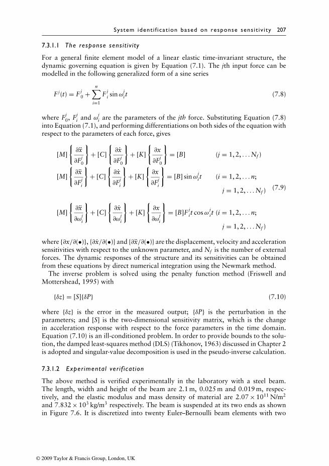
System ident i f i ca t ion based on response sens i t i v i ty 207
7.3.1.1 The response sens i t i v i t y
For a general finite element model of a linear elastic time-invariant structure, thedynamic governing equation is given by Equation (7.1). The jth input force can bemodelled in the following generalized form of a sine series
F j(t) = F j0 +
n∑i=1
F ji sinωj
i t (7.8)
where Fj0, Fj
i and ωji are the parameters of the jth force. Substituting Equation (7.8)
into Equation (7.1), and performing differentiations on both sides of the equation withrespect to the parameters of each force, gives
[M]
{∂x
∂Fj0
}+ [C]
{∂x
∂Fj0
}+ [K]
{∂x
∂Fj0
}= [B] (j = 1, 2, . . .Nf )
[M]
{∂x
∂Fji
}+ [C]
{∂x
∂Fji
}+ [K]
{∂x
∂Fji
}= [B] sinωj
i t (i = 1, 2, . . .n;
j = 1, 2, . . .Nf )
[M]
{∂x
∂ωji
}+ [C]
{∂x
∂ωji
}+ [K]
{∂x
∂ωji
}= [B]F j
it cosω jit (i = 1, 2, . . .n;
j = 1, 2, . . .Nf )
(7.9)
where {∂x/∂(•)}, {∂x/∂(•)} and {∂x/∂(•)} are the displacement, velocity and accelerationsensitivities with respect to the unknown parameter, and Nf is the number of externalforces. The dynamic responses of the structure and its sensitivities can be obtainedfrom these equations by direct numerical integration using the Newmark method.
The inverse problem is solved using the penalty function method (Friswell andMottershead, 1995) with
{δz} = [S]{δP} (7.10)
where {δz} is the error in the measured output; {δP} is the perturbation in theparameters; and [S] is the two-dimensional sensitivity matrix, which is the changein acceleration response with respect to the force parameters in the time domain.Equation (7.10) is an ill-conditioned problem. In order to provide bounds to the solu-tion, the damped least-squares method (DLS) (Tikhonov, 1963) discussed in Chapter 2is adopted and singular-value decomposition is used in the pseudo-inverse calculation.
7.3.1.2 Exper imenta l ver i f i cat ion
The above method is verified experimentally in the laboratory with a steel beam.The length, width and height of the beam are 2.1 m, 0.025 m and 0.019 m, respec-tively, and the elastic modulus and mass density of material are 2.07 × 10¹¹ N/m2
and 7.832 × 10³ kg/m3 respectively. The beam is suspended at its two ends as shownin Figure 7.6. It is discretized into twenty Euler–Bernoulli beam elements with two
© 2009 Taylor & Francis Group, London, UK
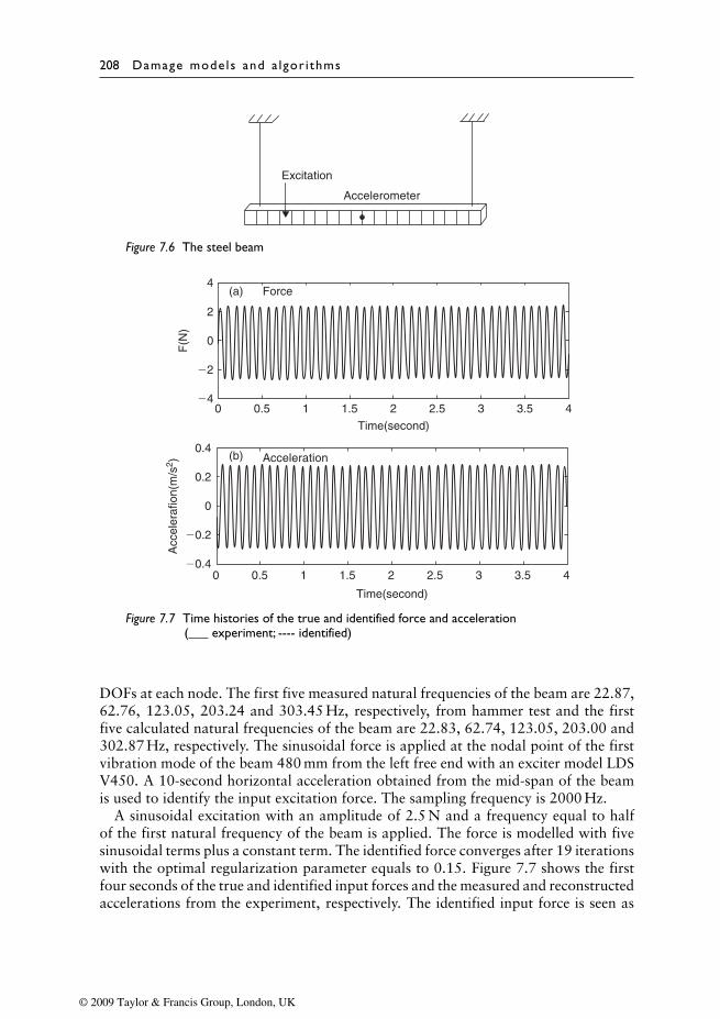
208 Damage mode ls and a lgor i thms
Accelerometer
Excitation
Figure 7.6 The steel beam
Force(a)
(b)
4
2
0
�2
�4
0.4
0 0.5 1 1.5 2 2.5 3 3.5 4
0 0.5 1 1.5 2
Time(second)
Time(second)
F(N
)A
ccel
eraf
ion(
m/s
2 )
2.5 3 3.5 4
0.2
0
�0.2
�0.4
Acceleration
Figure 7.7 Time histories of the true and identified force and acceleration(___ experiment; ---- identified)
DOFs at each node. The first five measured natural frequencies of the beam are 22.87,62.76, 123.05, 203.24 and 303.45 Hz, respectively, from hammer test and the firstfive calculated natural frequencies of the beam are 22.83, 62.74, 123.05, 203.00 and302.87 Hz, respectively. The sinusoidal force is applied at the nodal point of the firstvibration mode of the beam 480 mm from the left free end with an exciter model LDSV450. A 10-second horizontal acceleration obtained from the mid-span of the beamis used to identify the input excitation force. The sampling frequency is 2000 Hz.
A sinusoidal excitation with an amplitude of 2.5 N and a frequency equal to halfof the first natural frequency of the beam is applied. The force is modelled with fivesinusoidal terms plus a constant term. The identified force converges after 19 iterationswith the optimal regularization parameter equals to 0.15. Figure 7.7 shows the firstfour seconds of the true and identified input forces and the measured and reconstructedaccelerations from the experiment, respectively. The identified input force is seen as
© 2009 Taylor & Francis Group, London, UK
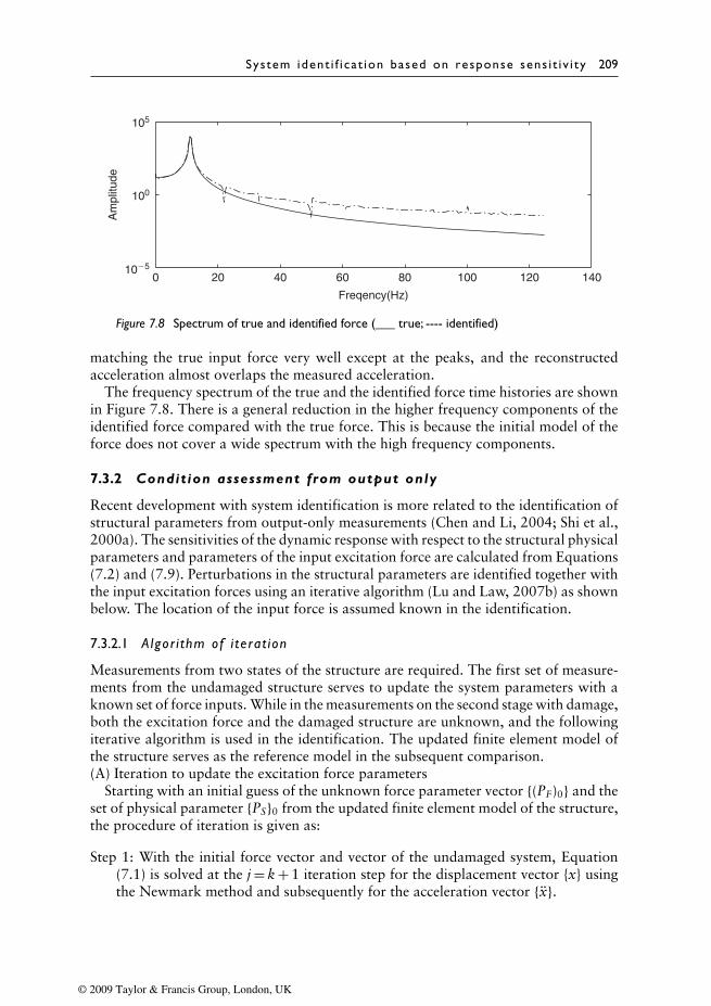
System ident i f i ca t ion based on response sens i t i v i ty 209
105
10�5
100
0 20 40 60 80 100 120 140
Freqency(Hz)
Am
plitu
de
Figure 7.8 Spectrum of true and identified force (___ true; ---- identified)
matching the true input force very well except at the peaks, and the reconstructedacceleration almost overlaps the measured acceleration.
The frequency spectrum of the true and the identified force time histories are shownin Figure 7.8. There is a general reduction in the higher frequency components of theidentified force compared with the true force. This is because the initial model of theforce does not cover a wide spectrum with the high frequency components.
7.3.2 Condit ion assessment from output only
Recent development with system identification is more related to the identification ofstructural parameters from output-only measurements (Chen and Li, 2004; Shi et al.,2000a). The sensitivities of the dynamic response with respect to the structural physicalparameters and parameters of the input excitation force are calculated from Equations(7.2) and (7.9). Perturbations in the structural parameters are identified together withthe input excitation forces using an iterative algorithm (Lu and Law, 2007b) as shownbelow. The location of the input force is assumed known in the identification.
7.3.2.1 Algor i thm of i terat ion
Measurements from two states of the structure are required. The first set of measure-ments from the undamaged structure serves to update the system parameters with aknown set of force inputs. While in the measurements on the second stage with damage,both the excitation force and the damaged structure are unknown, and the followingiterative algorithm is used in the identification. The updated finite element model ofthe structure serves as the reference model in the subsequent comparison.(A) Iteration to update the excitation force parameters
Starting with an initial guess of the unknown force parameter vector {(PF)0} and theset of physical parameter {PS}0 from the updated finite element model of the structure,the procedure of iteration is given as:
Step 1: With the initial force vector and vector of the undamaged system, Equation(7.1) is solved at the j = k + 1 iteration step for the displacement vector {x} usingthe Newmark method and subsequently for the acceleration vector {x}.
© 2009 Taylor & Francis Group, London, UK
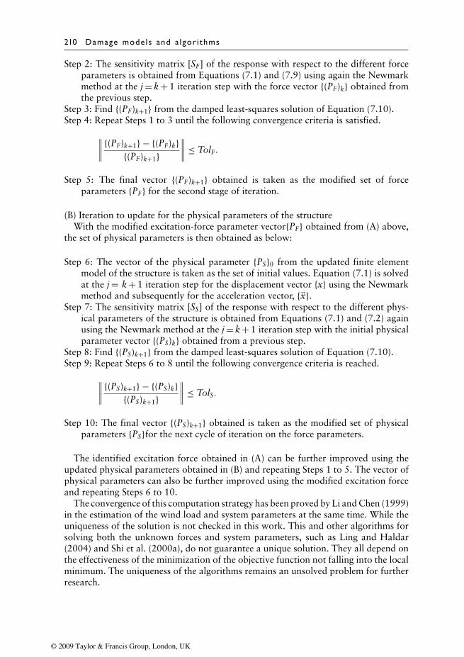
210 Damage mode ls and a lgor i thms
Step 2: The sensitivity matrix [SF] of the response with respect to the different forceparameters is obtained from Equations (7.1) and (7.9) using again the Newmarkmethod at the j = k + 1 iteration step with the force vector {(PF)k} obtained fromthe previous step.
Step 3: Find {(PF)k+1} from the damped least-squares solution of Equation (7.10).Step 4: Repeat Steps 1 to 3 until the following convergence criteria is satisfied.∥∥∥∥ {(PF)k+1} − {(PF)k}
{(PF)k+1}∥∥∥∥ ≤ TolF.
Step 5: The final vector {(PF)k+1} obtained is taken as the modified set of forceparameters {PF} for the second stage of iteration.
(B) Iteration to update for the physical parameters of the structureWith the modified excitation-force parameter vector{PF} obtained from (A) above,
the set of physical parameters is then obtained as below:
Step 6: The vector of the physical parameter {PS}0 from the updated finite elementmodel of the structure is taken as the set of initial values. Equation (7.1) is solvedat the j = k + 1 iteration step for the displacement vector {x} using the Newmarkmethod and subsequently for the acceleration vector, {x}.
Step 7: The sensitivity matrix [SS] of the response with respect to the different phys-ical parameters of the structure is obtained from Equations (7.1) and (7.2) againusing the Newmark method at the j = k + 1 iteration step with the initial physicalparameter vector {(PS)k} obtained from a previous step.
Step 8: Find {(PS)k+1} from the damped least-squares solution of Equation (7.10).Step 9: Repeat Steps 6 to 8 until the following convergence criteria is reached.∥∥∥∥ {(PS)k+1} − {(PS)k}
{(PS)k+1}∥∥∥∥ ≤ TolS.
Step 10: The final vector {(PS)k+1} obtained is taken as the modified set of physicalparameters {PS}for the next cycle of iteration on the force parameters.
The identified excitation force obtained in (A) can be further improved using theupdated physical parameters obtained in (B) and repeating Steps 1 to 5. The vector ofphysical parameters can also be further improved using the modified excitation forceand repeating Steps 6 to 10.
The convergence of this computation strategy has been proved by Li and Chen (1999)in the estimation of the wind load and system parameters at the same time. While theuniqueness of the solution is not checked in this work. This and other algorithms forsolving both the unknown forces and system parameters, such as Ling and Haldar(2004) and Shi et al. (2000a), do not guarantee a unique solution. They all depend onthe effectiveness of the minimization of the objective function not falling into the localminimum. The uniqueness of the algorithms remains an unsolved problem for furtherresearch.
© 2009 Taylor & Francis Group, London, UK
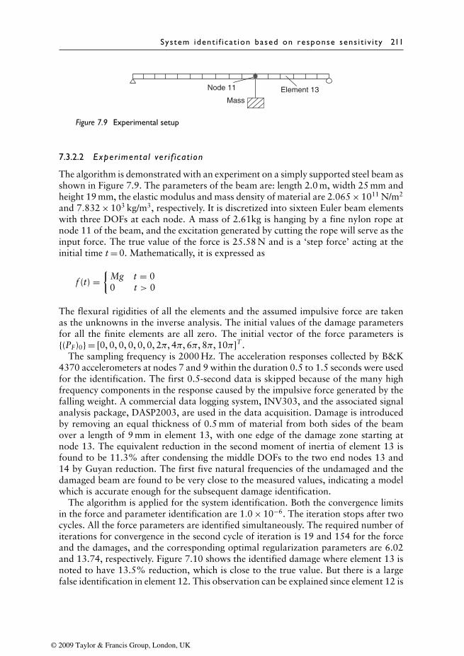
System ident i f i ca t ion based on response sens i t i v i ty 211
Element 13 Node 11
Mass
Figure 7.9 Experimental setup
7.3.2.2 Exper imenta l ver i f i cat ion
The algorithm is demonstrated with an experiment on a simply supported steel beam asshown in Figure 7.9. The parameters of the beam are: length 2.0 m, width 25 mm andheight 19 mm, the elastic modulus and mass density of material are 2.065 × 10¹¹ N/m2
and 7.832 × 10³ kg/m3, respectively. It is discretized into sixteen Euler beam elementswith three DOFs at each node. A mass of 2.61kg is hanging by a fine nylon rope atnode 11 of the beam, and the excitation generated by cutting the rope will serve as theinput force. The true value of the force is 25.58 N and is a ‘step force’ acting at theinitial time t = 0. Mathematically, it is expressed as
f (t) ={
Mg t = 00 t > 0
The flexural rigidities of all the elements and the assumed impulsive force are takenas the unknowns in the inverse analysis. The initial values of the damage parametersfor all the finite elements are all zero. The initial vector of the force parameters is{(PF)0} = [0, 0, 0, 0, 0, 0, 2π, 4π, 6π, 8π, 10π]T .
The sampling frequency is 2000 Hz. The acceleration responses collected by B&K4370 accelerometers at nodes 7 and 9 within the duration 0.5 to 1.5 seconds were usedfor the identification. The first 0.5-second data is skipped because of the many highfrequency components in the response caused by the impulsive force generated by thefalling weight. A commercial data logging system, INV303, and the associated signalanalysis package, DASP2003, are used in the data acquisition. Damage is introducedby removing an equal thickness of 0.5 mm of material from both sides of the beamover a length of 9 mm in element 13, with one edge of the damage zone starting atnode 13. The equivalent reduction in the second moment of inertia of element 13 isfound to be 11.3% after condensing the middle DOFs to the two end nodes 13 and14 by Guyan reduction. The first five natural frequencies of the undamaged and thedamaged beam are found to be very close to the measured values, indicating a modelwhich is accurate enough for the subsequent damage identification.
The algorithm is applied for the system identification. Both the convergence limitsin the force and parameter identification are 1.0 × 10⁻⁶. The iteration stops after twocycles. All the force parameters are identified simultaneously. The required number ofiterations for convergence in the second cycle of iteration is 19 and 154 for the forceand the damages, and the corresponding optimal regularization parameters are 6.02and 13.74, respectively. Figure 7.10 shows the identified damage where element 13 isnoted to have 13.5% reduction, which is close to the true value. But there is a largefalse identification in element 12. This observation can be explained since element 12 is
© 2009 Taylor & Francis Group, London, UK
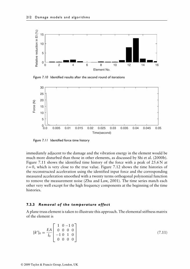
212 Damage mode ls and a lgor i thms
15
10
0
5
0 2 4 6 108 12 14 16
Element No.
Rel
ativ
e re
duct
ion
in E
l (%
)
Figure 7.10 Identified results after the second round of iterations
30
25
20
15
10
0
5
0.0 0.005 0.01 0.015 0.0250.02 0.03 0.040.035 0.045 0.05
Time(second)
For
ce (
N)
Figure 7.11 Identified force time history
immediately adjacent to the damage and the vibration energy in the element would bemuch more disturbed than those in other elements, as discussed by Shi et al. (2000b).Figure 7.11 shows the identified time history of the force with a peak of 25.6 N att = 0, which is very close to the true value. Figure 7.12 shows the time histories ofthe reconstructed acceleration using the identified input force and the correspondingmeasured acceleration smoothed with a twenty terms orthogonal polynomial functionto remove the measurement noise (Zhu and Law, 2001). The time series match eachother very well except for the high frequency components at the beginning of the timehistories.
7.3.3 Removal of the temperature effect
A plane truss element is taken to illustrate this approach. The elemental stiffness matrixof the element is
[ke]0 = EAl0
1 0 −1 00 0 0 0
−1 0 1 00 0 0 0
(7.11)
© 2009 Taylor & Francis Group, London, UK
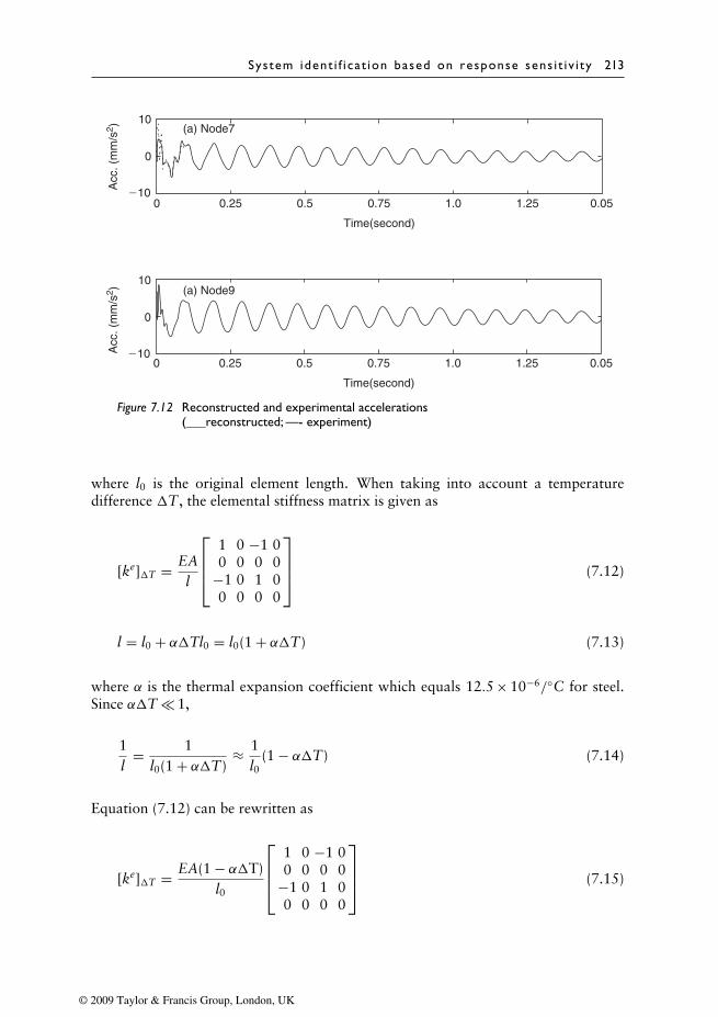
System ident i f i ca t ion based on response sens i t i v i ty 213
0 0.25 0.5 0.75 1.251.0 0.05
Time(second)
Acc
. (m
m/s
2 )A
cc. (
mm
/s2 )
10
0
�10
10(a) Node7
(a) Node9
0
�10
0 0.25 0.5 0.75 1.251.0 0.05
Time(second)
Figure 7.12 Reconstructed and experimental accelerations(___reconstructed; —- experiment)
where l0 is the original element length. When taking into account a temperaturedifference �T, the elemental stiffness matrix is given as
[ke]�T = EAl
1 0 −1 00 0 0 0
−1 0 1 00 0 0 0
(7.12)
l = l0 + α�Tl0 = l0(1 + α�T) (7.13)
where α is the thermal expansion coefficient which equals 12.5 × 10⁻⁶/◦C for steel.Since α�T 1,
1l
= 1l0(1 + α�T)
≈ 1l0
(1 − α�T) (7.14)
Equation (7.12) can be rewritten as
[ke]�T = EA(1 − α�T)l0
1 0 −1 00 0 0 0
−1 0 1 00 0 0 0
(7.15)
© 2009 Taylor & Francis Group, London, UK
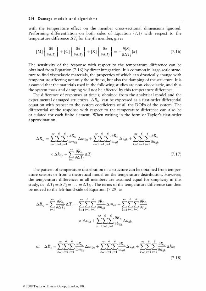
214 Damage mode ls and a lgor i thms
with the temperature effect on the member cross-sectional dimensions ignored.Performing differentiation on both sides of Equation (7.1) with respect to thetemperature difference �Tj for the jth member, gives
[M]{∂x∂�Tj
}+ [C]
{∂x∂�Tj
}+ [K]
{∂x∂�Tj
}= − ∂[K]
∂�Tj{x} (7.16)
The sensitivity of the response with respect to the temperature difference can beobtained from Equation (7.16) by direct integration. It is common in large-scale struc-ture to find viscoelastic materials, the properties of which can drastically change withtemperature affecting not only the stiffness, but also the damping of the structure. It isassumed that the materials used in the following studies are non-viscoelastic, and thusthe system mass and damping will not be affected by this temperature difference.
The difference of responses at time ti obtained from the analytical model and theexperimental damaged structures, �Rti , can be expressed as a first-order differentialequation with respect to the system coefficients of all the DOFs of the system. Thedifferential of the response with respect to the temperature difference can also becalculated for each finite element. When writing in the form of Taylor’s first-orderapproximation,
�Rti =ne∑
k=1
6∑i=1
6∑j=1
∂Rti
∂mijk�mijk +
ne∑k=1
6∑i=1
6∑j=1
∂Rti
∂cijk�cijk +
ne∑k=1
6∑i=1
6∑j=1
∂Rti
∂kijk
×�kijk +ne∑
j=1
∂Rti
∂�Tj�Tj (7.17)
The pattern of temperature distribution in a structure can be obtained from temper-ature sensors or from a theoretical model on the temperature distribution. However,the temperature differences in all members are assumed equal for simplicity in thisstudy, i.e. �T1 =�T2 = . . . =�TN . The terms of the temperature difference can thenbe moved to the left-hand-side of Equation (7.29) as
�Rti −ne∑
j=1
∂Rti
∂�Tj�Tj =
ne∑k=1
6∑i=1
6∑j=1
∂Rti
∂mijk�mijk +
ne∑k=1
6∑i=1
6∑j=1
∂Rti
∂cijk
×�cijk +ne∑
k=1
6∑i=1
6∑j=1
∂Rti
∂kijk�kijk
or �R′ti =
ne∑k=1
6∑i=1
6∑j=1
∂Rti
∂mijk�mijk +
ne∑k=1
6∑i=1
6∑j=1
∂Rti
∂cijk�cijk +
ne∑k=1
6∑i=1
6∑j=1
∂Rti
∂kijk�kijk
(7.18)
© 2009 Taylor & Francis Group, London, UK
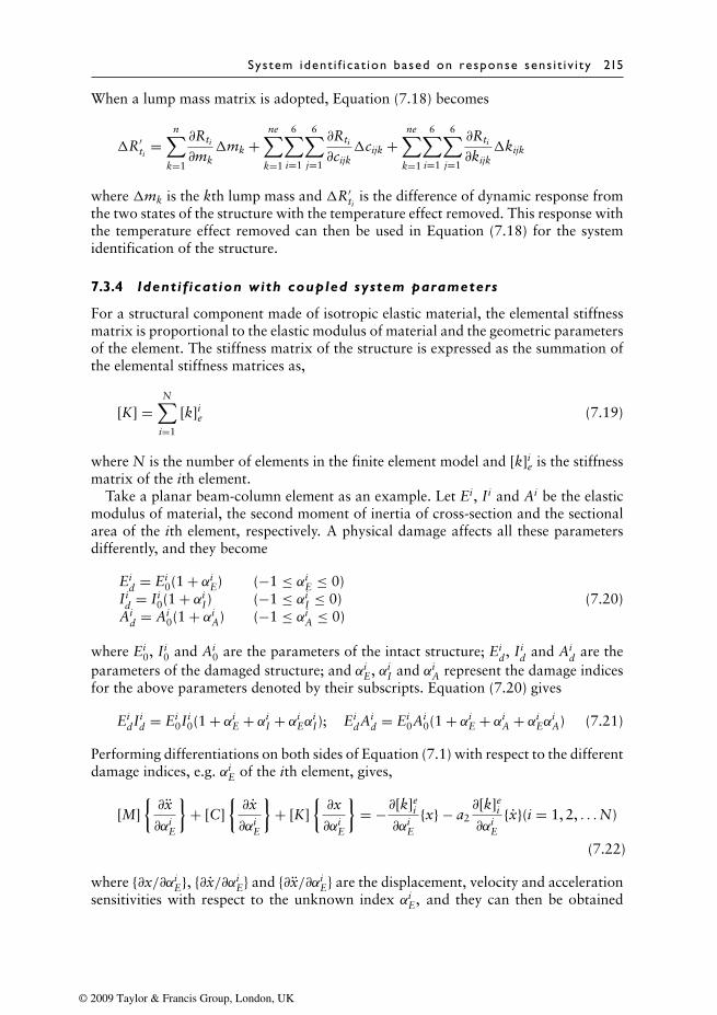
System ident i f i ca t ion based on response sens i t i v i ty 215
When a lump mass matrix is adopted, Equation (7.18) becomes
�R′ti =
n∑k=1
∂Rti
∂mk�mk +
ne∑k=1
6∑i=1
6∑j=1
∂Rti
∂cijk�cijk +
ne∑k=1
6∑i=1
6∑j=1
∂Rti
∂kijk�kijk
where �mk is the kth lump mass and �R′ti is the difference of dynamic response from
the two states of the structure with the temperature effect removed. This response withthe temperature effect removed can then be used in Equation (7.18) for the systemidentification of the structure.
7.3.4 Identif ication with coupled system parameters
For a structural component made of isotropic elastic material, the elemental stiffnessmatrix is proportional to the elastic modulus of material and the geometric parametersof the element. The stiffness matrix of the structure is expressed as the summation ofthe elemental stiffness matrices as,
[K] =N∑
i=1
[k]ie (7.19)
where N is the number of elements in the finite element model and [k]ie is the stiffness
matrix of the ith element.Take a planar beam-column element as an example. Let Ei, Ii and Ai be the elastic
modulus of material, the second moment of inertia of cross-section and the sectionalarea of the ith element, respectively. A physical damage affects all these parametersdifferently, and they become
Eid = Ei
0(1 + αiE) (−1 ≤ αi
E ≤ 0)Ii
d = Ii0(1 + αi
I) (−1 ≤ αiI ≤ 0)
Aid = Ai
0(1 + αiA) (−1 ≤ αi
A ≤ 0)(7.20)
where Ei0, Ii
0 and Ai0 are the parameters of the intact structure; Ei
d, Iid and Ai
d are theparameters of the damaged structure; and αi
E, αiI and αi
A represent the damage indicesfor the above parameters denoted by their subscripts. Equation (7.20) gives
EidIi
d = Ei0Ii
0(1 + αiE + αi
I + αiEα
iI); Ei
dAid = Ei
0Ai0(1 + αi
E + αiA + αi
EαiA) (7.21)
Performing differentiations on both sides of Equation (7.1) with respect to the differentdamage indices, e.g. αi
E of the ith element, gives,
[M]{∂x
∂αiE
}+ [C]
{∂x
∂αiE
}+ [K]
{∂x
∂αiE
}= −∂[k]e
i
∂αiE
{x} − a2∂[k]e
i
∂αiE
{x}(i = 1, 2, . . .N)
(7.22)
where {∂x/∂αiE}, {∂x/∂αi
E} and {∂x/∂αiE} are the displacement, velocity and acceleration
sensitivities with respect to the unknown index αiE, and they can then be obtained
© 2009 Taylor & Francis Group, London, UK
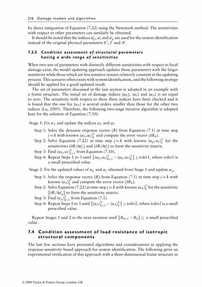
216 Damage mode ls and a lgor i thms
by direct integration of Equation (7.22) using the Newmark method. The sensitivitieswith respect to other parameters can similarly be obtained.
It should be noted that the indices αiE, αi
I and αiA are used for the system identification
instead of the original physical parameters Ei, Ii and Ai.
7.3.5 Condit ion assessment of structural parametershaving a wide range of sensit iv it ies
When two sets of parameters with distinctly different sensitivities with respect to localdamage exist, the model updating approach updates those parameters with the largersensitivity while those which are less sensitive remain relatively constant in the updatingprocess. This scenario often exists with system identification, and the following strategyshould be applied for a good updated result.
The set of parameters discussed in the last section is adopted in an example witha frame structure. The initial set of damage indices {αE}, {αI} and {αA} is set equalto zero. The sensitivity with respect to these three indices have been checked and itis found that the one for {αA} is several orders smaller than those for the other twoindices (Lu, 2005). Therefore, the following two-stage iterative algorithm is adoptedhere for the solution of Equation (7.10):
Stage 1: Fix αA and update the indices αE and αI.
Step 1: Solve the dynamic response vector {R} from Equation (7.1) at time stepj = k with known (αE,αI)T
k and compute the error vector {δRk}.Step 2: Solve Equation (7.22) at time step j = k with known (αE,αI)T
k for thesensitivities {∂R/∂αi
E} and {∂R/∂αi
I} to form the sensitivity matrix.
Step 3: Find (αE,αI)Tk+1 from Equation (7.10).
Step 4: Repeat Steps 1 to 3 until∥∥(αE,αI)T
k+1 − (αE,αI)Tk
∥∥≤ toler1, where toler1 isa small prescribed value.
Stage 2: Fix the updated values of αE and αI obtained from Stage 1 and update αA.
Step 1: Solve the response vector {R} from Equation (7.1) at time step j = k withknown (αA)T
k and compute the error vector {δRk}.Step 2: Solve Equation (7.22) at time step j = k with known (αA)T
k for the sensitivity{∂R/∂αi
A
}to form the sensitivity matrix.
Step 3: Find (αA)Tk+1 from Equation (7.1).
Step 4: Repeat Steps 1 to 3 until∥∥(αA)T
k+1 − (αA)Tk
∥∥≤ toler2, where toler2 is a smallprescribed value.
Repeat Stages 1 and 2 in the next iteration until∥∥Rk+1 − Rk
∥∥≤ a small prescribedvalue.
7.4 Condition assessment of load resistance of isotropicstructural components
The last few sections have presented algorithms and considerations in applying theresponse-sensitivity based approach for system identification. The following gives anexperimental verification of this approach with a three-dimensional frame structure in
© 2009 Taylor & Francis Group, London, UK
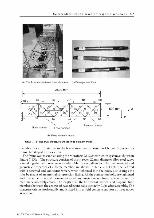
System ident i f i ca t ion based on response sens i t i v i ty 217
(b) Finite element model
(a) The five-bay cantilever truss structure (c) Damage members
N2 N3 N4 N5 N6
N7 N8 N9 N10 N11 N12
N14 N15 N16N17
1 2 3 4 5
6 7 8 9 10
11 12 13 1415 16 17 18 19
20
21
22
23
24
25
26
27
28
29
30
31
32
33
34
35
36
37
Node number Element number
x
z
2500 mm
500 mm
Local damage
N13
N1
Figure 7.13 The truss structure and its finite element model
the laboratory. It is similar to the frame structure discussed in Chapter 3 but with atriangular-shaped cross-section.
The frame was assembled using the Meroform M12 construction system as shown inFigure 7.13(a). The structure consists of thirty-seven 22 mm diameter alloy steel tubesjointed together with seventeen standard Meroform ball nodes. The main material andgeometric properties of a frame member are shown in Table 7.1. Each tube is fittedwith a screwed end connector which, when tightened into the node, also clamps thetube by means of an internal compression fitting. All the connection bolts are tightenedwith the same torsional moment to avoid asymmetry or nonlinear effects caused byman-made assembly errors. The length of all the horizontal, vertical and diagonal tubemembers between the centres of two adjacent balls is exactly 0.5m after assembly. Thestructure orients horizontally and is fixed into a rigid concrete support at three nodesat one end.
© 2009 Taylor & Francis Group, London, UK
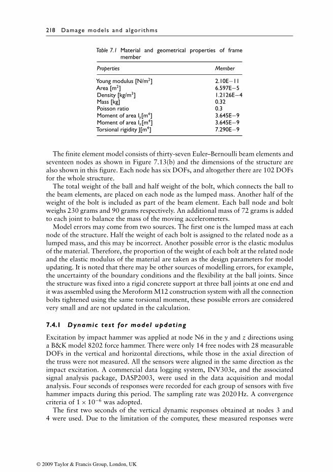
218 Damage mode ls and a lgor i thms
Table 7.1 Material and geometrical properties of framemember
Properties Member
Young modulus [N/m2] 2.10E−11Area [m2] 6.597E−5Density [kg/m3] 1.2126E−4Mass [kg] 0.32Poisson ratio 0.3Moment of area Iy[m4] 3.645E−9Moment of area Iz[m4] 3.645E−9Torsional rigidity J[m4] 7.290E−9
The finite element model consists of thirty-seven Euler–Bernoulli beam elements andseventeen nodes as shown in Figure 7.13(b) and the dimensions of the structure arealso shown in this figure. Each node has six DOFs, and altogether there are 102 DOFsfor the whole structure.
The total weight of the ball and half weight of the bolt, which connects the ball tothe beam elements, are placed on each node as the lumped mass. Another half of theweight of the bolt is included as part of the beam element. Each ball node and boltweighs 230 grams and 90 grams respectively. An additional mass of 72 grams is addedto each joint to balance the mass of the moving accelerometers.
Model errors may come from two sources. The first one is the lumped mass at eachnode of the structure. Half the weight of each bolt is assigned to the related node as alumped mass, and this may be incorrect. Another possible error is the elastic modulusof the material. Therefore, the proportion of the weight of each bolt at the related nodeand the elastic modulus of the material are taken as the design parameters for modelupdating. It is noted that there may be other sources of modelling errors, for example,the uncertainty of the boundary conditions and the flexibility at the ball joints. Sincethe structure was fixed into a rigid concrete support at three ball joints at one end andit was assembled using the Meroform M12 construction system with all the connectionbolts tightened using the same torsional moment, these possible errors are consideredvery small and are not updated in the calculation.
7.4.1 Dynamic test for model updating
Excitation by impact hammer was applied at node N6 in the y and z directions usinga B&K model 8202 force hammer. There were only 14 free nodes with 28 measurableDOFs in the vertical and horizontal directions, while those in the axial direction ofthe truss were not measured. All the sensors were aligned in the same direction as theimpact excitation. A commercial data logging system, INV303e, and the associatedsignal analysis package, DASP2003, were used in the data acquisition and modalanalysis. Four seconds of responses were recorded for each group of sensors with fivehammer impacts during this period. The sampling rate was 2020 Hz. A convergencecriteria of 1 × 10⁻⁶ was adopted.
The first two seconds of the vertical dynamic responses obtained at nodes 3 and4 were used. Due to the limitation of the computer, these measured responses were
© 2009 Taylor & Francis Group, London, UK

System ident i f i ca t ion based on response sens i t i v i ty 219
re-sampled to have a sampling rate of 505 Hz. There are two unknown parametersin the first stage of updating, which is much smaller than the 505 × 2 × 2 equationsformed from the measured responses. Results show that 62.5% of the weight of eachbolt should be placed at the related node as a lumped mass and the elastic modulus ofmaterial is 99.3% of the original value. The first eleven updated natural frequenciesagree well with the measured natural frequencies with a maximum relative error of1.86%. The calculated and the experimental mode shapes were also checked with theModal Assurance Criteria (Moller and Friberg, 1998) and the two sets of mode shapesmatch each other very well. These show that the updated finite element model canaccurately represent the intact structure for the next stage of damage detection.
7.4.2 Damage scenarios
Local faults are introduced by replacing intact members with damaged ones. Theartificial damage is of two types. Type I is a perforated slot cut in the central length ofthe member. The slot is 134.77 mm long, and the remaining depth of the tube in thecut-cross-section is 14.75 mm. Type II is the removal of a layer of material from thesurface of the member. The external diameter of the tube is reduced from 22.02 mmto 21.47 mm, and the weakened section is 202 mm long, located in the middle of thebeam leaving 99 mm and 75 mm length of original tube cross-section on both sides.Figure 7.13(c) gives a close up view of the damaged frame members.
Damage scenario E1 has Type II damage in the fourth member. Damage scenario E2includes an additional Type I damage in the second element. The slot opens vertically(global z-direction). Damage scenario E3 is similar to the last scenario but with theslot in element two opened horizontally (global y-direction). The equivalent damagescomputed by the Guyon method are listed in Table 7.2. Each of the above scenariosinvolves four types of damage in the beam element, i.e. a reduction in cross-sectionalarea A, the polar moment of inertia J and the moment of inertia Iz and Iy.
7.4.3 Dynamic test for damage detection
A falling weight test was then conducted on the structure for each damage scenario.A 5.15 kg mass was hung at node N17. Free vibration was introduced by a suddenrelease of the mass. The time histories from selected accelerometers were recorded.These responses were intentionally selected to be not in close proximity to the dam-aged elements. The sampling rate was 2020 Hz and the time duration was 8 secondsfor each test covering the whole duration of vibration caused by the falling weightexcitation. The orthogonal polynomial function (Zhu and Law, 2001) was used toremove the measurement noise in the acceleration data. The required iteration numberfor convergence and the corresponding optimal regularization parameter are shown inTable 7.3.
Damage scenario E1
Only data in the first two seconds of the response from two accelerometers (node 3,z-direction and node 11, y-direction) were used for the damage identification. Themeasured acceleration was re-sampled at 505 Hz.
Four sets of damage indices, namely, αJ ,αIy , αIz and αA were updated with a totalof 37 × 4 = 148 unknowns, which is smaller than 505 × 2 × 2 equations. Figure 7.14
© 2009 Taylor & Francis Group, London, UK
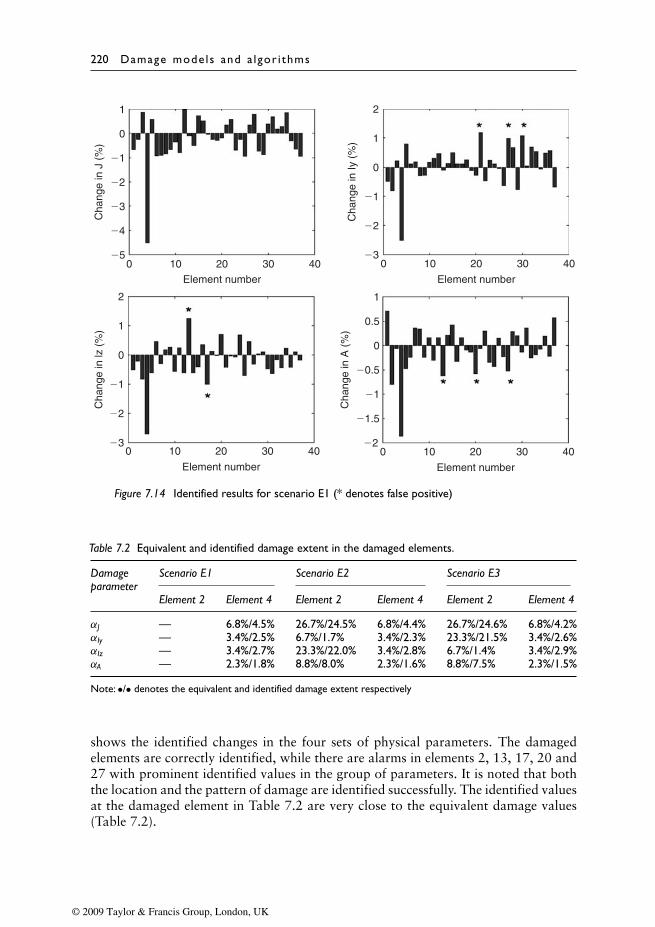
220 Damage mode ls and a lgor i thms
1
0
�1
�2
�3
�4
�50 10 20 30
Element number Element number
40 0 10 20 30 40
Element number
Cha
nge
in J
(%
)C
hang
e in
lz (
%)
Cha
nge
in A
(%
)C
hang
e in
Iy (
%)
0 10 20 30 40Element number
0 10 20 30 40
1
2
0
�1
�2
�3
1
2
0
�1
�2
�3
0.5
1
0
�0.5
�1
�1.5
�2
Figure 7.14 Identified results for scenario E1 (* denotes false positive)
Table 7.2 Equivalent and identified damage extent in the damaged elements.
Damage Scenario E1 Scenario E2 Scenario E3parameter
Element 2 Element 4 Element 2 Element 4 Element 2 Element 4
αJ — 6.8%/4.5% 26.7%/24.5% 6.8%/4.4% 26.7%/24.6% 6.8%/4.2%αIy — 3.4%/2.5% 6.7%/1.7% 3.4%/2.3% 23.3%/21.5% 3.4%/2.6%αIz — 3.4%/2.7% 23.3%/22.0% 3.4%/2.8% 6.7%/1.4% 3.4%/2.9%αA — 2.3%/1.8% 8.8%/8.0% 2.3%/1.6% 8.8%/7.5% 2.3%/1.5%
Note: •/• denotes the equivalent and identified damage extent respectively
shows the identified changes in the four sets of physical parameters. The damagedelements are correctly identified, while there are alarms in elements 2, 13, 17, 20 and27 with prominent identified values in the group of parameters. It is noted that boththe location and the pattern of damage are identified successfully. The identified valuesat the damaged element in Table 7.2 are very close to the equivalent damage values(Table 7.2).
© 2009 Taylor & Francis Group, London, UK
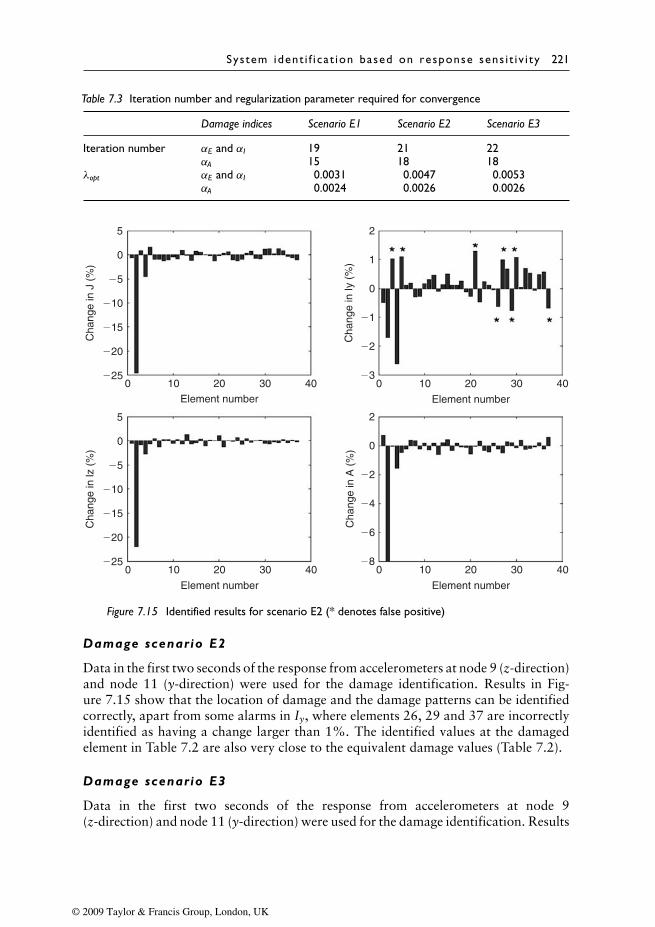
System ident i f i ca t ion based on response sens i t i v i ty 221
Table 7.3 Iteration number and regularization parameter required for convergence
Damage indices Scenario E1 Scenario E2 Scenario E3
Iteration number αE and αI 19 21 22αA 15 18 18
λopt αE and αI 0.0031 0.0047 0.0053αA 0.0024 0.0026 0.0026
5
0
�5
�10
�15
�20
�25
5
0
�5
�10
�15
�20
�25
0 10 20 30
Element number Element number
40 0 10 20 30 40
Element number
Cha
nge
in J
(%
)C
hang
e in
lz (
%)
Cha
nge
in A
(%
)C
hang
e in
Iy (
%)
0 10 20 30 40
Element number
0 10 20 30 40
1
2
0
�1
�2
�3
0
2
�4
�2
�6
�8
Figure 7.15 Identified results for scenario E2 (* denotes false positive)
Damage scenario E2
Data in the first two seconds of the response from accelerometers at node 9 (z-direction)and node 11 (y-direction) were used for the damage identification. Results in Fig-ure 7.15 show that the location of damage and the damage patterns can be identifiedcorrectly, apart from some alarms in Iy, where elements 26, 29 and 37 are incorrectlyidentified as having a change larger than 1%. The identified values at the damagedelement in Table 7.2 are also very close to the equivalent damage values (Table 7.2).
Damage scenario E3
Data in the first two seconds of the response from accelerometers at node 9(z-direction) and node 11 (y-direction) were used for the damage identification. Results
© 2009 Taylor & Francis Group, London, UK
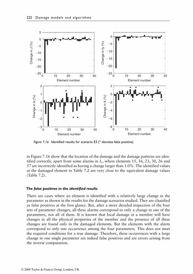
222 Damage mode ls and a lgor i thms
5
0
�5
�10
�15
�20
�25
0
�5
�10
�15
�20
�250 10 20 30
Element number Element number
40 0 10 20 30 40
Element number
Cha
nge
in J
(%
)C
hang
e in
lz (
%)
Cha
nge
in A
(%
)C
hang
e in
Iy (
%)
0 10 20 30 40
Element number
0 10 20 30 40
1
2
0
�1
�2
�3
0
2
�4
�2
�6
�8
Figure 7.16 Identified results for scenario E3 (* denotes false positive)
in Figure 7.16 show that the location of the damage and the damage patterns are iden-tified correctly, apart from some alarms in Iz, where elements 15, 16, 23, 30, 26 and37 are incorrectly identified as having a change larger than 1.0%. The identified valuesat the damaged element in Table 7.2 are very close to the equivalent damage values(Table 7.2).
The false positives in the identified results
There are cases where an element is identified with a relatively large change in theparameter as shown in the results for the damage scenarios studied. They are classifiedas false positives at the first glance. But, after a more detailed inspection of the foursets of parameter changes, all these alarms correspond to only a change in one of theparameters, not all of them. It is known that local damage in a member will havechanges in all the physical properties of the member and the presence of all thesechanges are found only in the damaged elements. But the elements with the alarmcorrespond to only one occurrence among the four parameters. This does not meetthe required conditions for a true damage. Therefore, these occurrences with a largechange in one single parameter are indeed false positives and are errors arising fromthe inverse computation.
© 2009 Taylor & Francis Group, London, UK
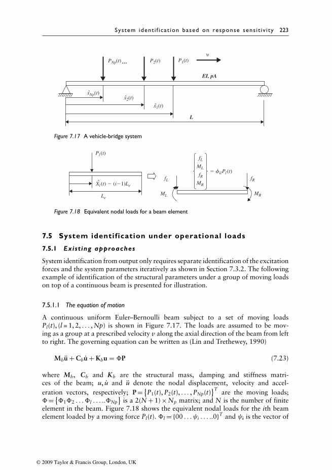
System ident i f i ca t ion based on response sens i t i v i ty 223
L
x2(t)
x1(t)
P1(t)P2(t)�
xNp(t)
PNp(t)
EI, pA
…
Figure 7.17 A vehicle-bridge system
� filPl (t)
Pl (t)
Xl (t) � (i�1)Le
fL
fL
ML
MLLe
fR fRMR
MR
Figure 7.18 Equivalent nodal loads for a beam element
7.5 System identification under operational loads
7.5.1 Exist ing approaches
System identification from output only requires separate identification of the excitationforces and the system parameters iteratively as shown in Section 7.3.2. The followingexample of identification of the structural parameters under a group of moving loadson top of a continuous beam is presented for illustration.
7.5.1.1 The equation of motion
A continuous uniform Euler–Bernoulli beam subject to a set of moving loadsPl(t), (l = 1, 2, . . . , Np) is shown in Figure 7.17. The loads are assumed to be mov-ing as a group at a prescribed velocity v along the axial direction of the beam from leftto right. The governing equation can be written as (Lin and Trethewey, 1990)
Mbu + Cbu + Kbu = �P (7.23)
where Mb, Cb and Kb are the structural mass, damping and stiffness matri-ces of the beam; u, u and u denote the nodal displacement, velocity and accel-eration vectors, respectively; P = {
P1(t), P2(t), . . . , PNp(t)}T are the moving loads;
�= {�1�2 . . . �l . . . ..�Np
}is a 2(N + 1) × Np matrix; and N is the number of finite
element in the beam. Figure 7.18 shows the equivalent nodal loads for the ith beamelement loaded by a moving force Pl(t). �l = {00 . . . ψi . . . ..0}T and ψi is the vector of
© 2009 Taylor & Francis Group, London, UK
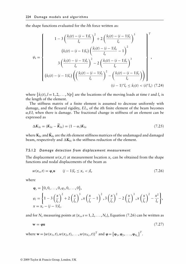
224 Damage mode ls and a lgor i thms
the shape functions evaluated for the lth force written as:
ψi =
1 − 3(
xl(t) − (i − 1)lele
)2
+ 2(
xl(t) − (i − 1)lele
)3
(xl(t) − (i − 1)le
) ( xl(t) − (i − 1)lele
− 1)2
3(
xl(t) − (i − 1)lele
)2
− 2(
xl(t) − (i − 1)lele
)3
(xl(t) − (i − 1)le
) (( xl(t) − (i − 1)lele
)2
−(
xl(t) − (i − 1)lele
))
T
,
((i − 1)∗le ≤ xl(t) < (i)∗le) (7.24)
where{xl(t), l = 1, 2, . . . , Np
}are the locations of the moving loads at time t and le is
the length of the element.The stiffness matrix of a finite element is assumed to decrease uniformly with
damage, and the flexural rigidity, EIi, of the ith finite element of the beam becomesαiEIi when there is damage. The fractional change in stiffness of an element can beexpressed as
�Kbi = (Kbi − Kbi) = (1 − αi)Kbi (7.25)
where Kbi and Kbi are the ith element stiffness matrices of the undamaged and damagedbeam, respectively and �Kbi is the stiffness reduction of the element.
7.5.1.2 Damage detect ion f rom disp lacement measurement
The displacement w(x, t) at measurement location xs can be obtained from the shapefunctions and nodal displacements of the beam as
w(xs, t) = ϕsu (j − 1)le ≤ xs < jle (7.26)
where
ϕs = {0, 0, . . . , 0,ϕj, 0, . . . , 0
},
ϕj ={
1 − 3(
xle
)2
+ 2(
xle
)3
, x(
xle
− 1)2
, 3(
xle
)2
− 2(
xle
)3
, x(
xle
)2
− x2
le
},
x = xs − (j − 1)le.
and for Ns measuring points at {xs, s = 1, 2, . . . , Ns}, Equation (7.26) can be written as
w = ϕu (7.27)
where w = {w(x1, t), w(x2, t), . . . , w(xNs , t)}T and ϕ = {ϕ1, ϕ2, . . . , ϕNs
}T .
© 2009 Taylor & Francis Group, London, UK
System ident i f i ca t ion based on response sens i t i v i ty 225
The nodal responses in Equation (7.27) can be written as
u = (ϕTϕ)−1ϕTw (7.28)
and the required u and u can be obtained using the orthogonal function expansion(Zhu and Law, 2001). The strain at point xs and time t can be written as
ε(xs, t) = −z∂2w(xs, t)∂x2
(7.29)
where z represents the distance from the neutral axis of the beam to the bottom surface.Similar to Equation (7.27), Equation (7.29) can be written in matrix form as
ε = ϕ′′u (7.30)
where ε = {ε(x1, t), ε(x2, t), . . . , ε(xNs , t)}T .
ϕ′′s = {0, 0, . . . ,ϕ′′
j , 0, . . . , 0};
ϕ′′j
={− 6
l2e
+ 12xl3e
,6xl2e
− 4le
,6l2e
− 12xl3e
,6xl2e
− 2le
};
x = xs − (j − 1)le
Similar to Equation (7.25), the equation of motion of the damaged beam under movingloads can be written as
Mbu + Cbu + f(u) = �P(t) (7.31)
where f(u) is the elastic restoring force of the system, and
f(u) = Kbu (7.32)
From Equation (7.31), the moving loads can be obtained as follow if the restoringforces are known
P(t) = (ΦTΦ)−1ΦT [Mu + Cu + f(u)] (7.33)
where I is the unity matrix. The moving loads in Equation (7.31) can be obtained fromEquation (7.10) using the damped least-squares method. And the element damageindex matrix is obtained from Equation (7.25) after the moving loads are identifiedfrom minimizing the following function
J(α) = ∥∥F(u) − f (u)∥∥2 (7.34)
where F(u) = ΦPidentify(t) − Mu − Cu; and Pidentify(t) is the set of identified moving loadsfrom the last iteration of the moving load identification.
Since the restoring forces and moving loads are all unknown, the iterative algorithmshown below is adopted to solve the problem (Zhu and Law, 2007a).
© 2009 Taylor & Francis Group, London, UK
226 Damage mode ls and a lgor i thms
1. Calculate the nodal displacements or strains from measurements by Equation(7.27) or (7.30).
2. Use the orthogonal function expansion to calculate the nodal velocity and acceler-ations. Twenty terms in the expansion is recommended for modelling the movingloads.
3. Initially assume there is no damage in the beam: α0 = {1, 1, . . . , 1}T .4. Identify the moving loads Pidentify(t) from the measured responses using Equation
(7.10) with regularization (Zhu and Law, 2002).5. Calculate the elastic restoring forces from F(u) = ΦPidentify(t) − Mu − Cu.6. Identify the damage index using Equations (7.25) and (7.34).7. Calculate the error for convergence:
Error1 = ‖Pi+1 − Pi‖‖Pi‖ × 100%, Error2 = ‖αi+1 − αi‖
‖αi‖ × 100%
Convergence is achieved when the sum of these two errors is a minimum.8. When the computed errors do not converge, repeat Steps 4 to 7.
7.5.2 The general ized orthogonal function expansion
The excitation was modelled in the generalized form of a sine series in Section 7.3.1,and the identification was successful using five terms in the series. But in the case ofa moving force, which is a function of both space and time, the modelling with a sineseries would be cumbersome. A more general form of representation is presented inthis section, which is in the form of a generalized orthogonal function expansion.
The excitation force f (t) in the time period [0, T] can be expressed in terms of a
Chebyshev series, f (t) =Nf∑i=1
CiTi(t) t ∈ [0, T], where Ti(t) is the first kind of orthogonal
Chebyshev polynomial, and
T1(t) = 1√
π, T2(t) =
√2π
(2T
t − 1)
T3(t) =√
2π
[2(
2T
t − 1)2
− 1
], . . ., Ti+1 (t) = 2
(2T
t − 1)
Ti (t)− Ti−1 (t)
(7.35)
where Nf is the degree of the polynomial and {Ci, i = 1, 2, . . .Nf } is the vector of coef-ficients in the expansion. The frequency component of the forcing function can bemodified by adopting different numbers of terms in the orthogonal function. The sen-sitivities of each of these coefficients, Ci, with respect to the different system parameterscan be found from equations similar to Equation (7.9) for the damage detection.
© 2009 Taylor & Francis Group, London, UK
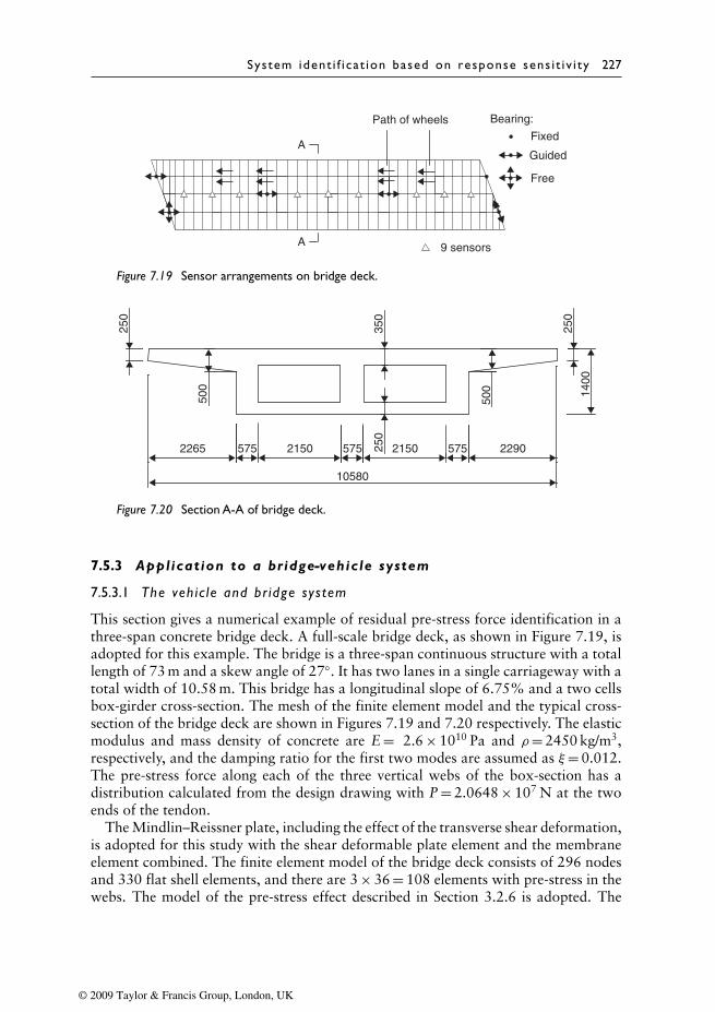
System ident i f i ca t ion based on response sens i t i v i ty 227
Path of wheels Bearing:
Fixed
Guided
Free
A
A 9 sensors
Figure 7.19 Sensor arrangements on bridge deck.
5752265 2150 575 2150 575 2290
500
500
350
250
250
1400
250
10580
Figure 7.20 Section A-A of bridge deck.
7.5.3 Application to a bridge-vehicle system
7.5.3.1 The veh ic le and br idge sys tem
This section gives a numerical example of residual pre-stress force identification in athree-span concrete bridge deck. A full-scale bridge deck, as shown in Figure 7.19, isadopted for this example. The bridge is a three-span continuous structure with a totallength of 73 m and a skew angle of 27◦. It has two lanes in a single carriageway with atotal width of 10.58 m. This bridge has a longitudinal slope of 6.75% and a two cellsbox-girder cross-section. The mesh of the finite element model and the typical cross-section of the bridge deck are shown in Figures 7.19 and 7.20 respectively. The elasticmodulus and mass density of concrete are E = 2.6 × 10¹⁰ Pa and ρ= 2450 kg/m3,respectively, and the damping ratio for the first two modes are assumed as ξ= 0.012.The pre-stress force along each of the three vertical webs of the box-section has adistribution calculated from the design drawing with P = 2.0648 × 10⁷ N at the twoends of the tendon.
The Mindlin–Reissner plate, including the effect of the transverse shear deformation,is adopted for this study with the shear deformable plate element and the membraneelement combined. The finite element model of the bridge deck consists of 296 nodesand 330 flat shell elements, and there are 3 × 36 = 108 elements with pre-stress in thewebs. The model of the pre-stress effect described in Section 3.2.6 is adopted. The
© 2009 Taylor & Francis Group, London, UK
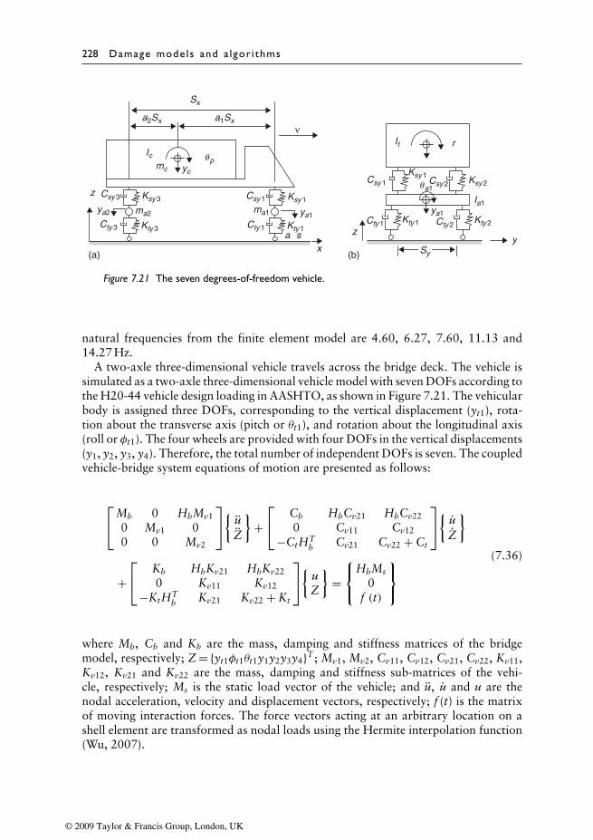
228 Damage mode ls and a lgor i thms
Sx
IcIt r
Ia1ya1
mc yc
Ksy 3 Ksy 1
Ksy 2Ksy 1
Kty 3Cty 3
Csy 3 Csy 1
Csy 1 Csy 2
Kty 1Kty 1 Kty 2
xy
z
z
ν
a sCty 1
Cty 1 Cty 2
ya2 ma2 ya1ma1
up
ua1
a2Sx a1Sx
Sy(a) (b)
Figure 7.21 The seven degrees-of-freedom vehicle.
natural frequencies from the finite element model are 4.60, 6.27, 7.60, 11.13 and14.27 Hz.
A two-axle three-dimensional vehicle travels across the bridge deck. The vehicle issimulated as a two-axle three-dimensional vehicle model with seven DOFs according tothe H20-44 vehicle design loading in AASHTO, as shown in Figure 7.21. The vehicularbody is assigned three DOFs, corresponding to the vertical displacement (yt1), rota-tion about the transverse axis (pitch or θt1), and rotation about the longitudinal axis(roll or φt1). The four wheels are provided with four DOFs in the vertical displacements(y1, y2, y3, y4). Therefore, the total number of independent DOFs is seven. The coupledvehicle-bridge system equations of motion are presented as follows:
Mb 0 HbMv1
0 Mv1 00 0 Mv2
{ uZ
}+ Cb HbCv21 HbCv22
0 Cv11 Cv12
−CtHTb Cv21 Cv22 + Ct
{ uZ
}
+ Kb HbKv21 HbKv22
0 Kv11 Kv12
−KtHTb Kv21 Kv22 + Kt
{ uZ
}=
HbMs
0f (t)
(7.36)
where Mb, Cb and Kb are the mass, damping and stiffness matrices of the bridgemodel, respectively; Z = {yt1φt1θt1y1y2y3y4}T ; Mv1, Mv2, Cv11, Cv12, Cv21, Cv22, Kv11,Kv12, Kv21 and Kv22 are the mass, damping and stiffness sub-matrices of the vehi-cle, respectively; Ms is the static load vector of the vehicle; and u, u and u are thenodal acceleration, velocity and displacement vectors, respectively; f (t) is the matrixof moving interaction forces. The force vectors acting at an arbitrary location on ashell element are transformed as nodal loads using the Hermite interpolation function(Wu, 2007).
© 2009 Taylor & Francis Group, London, UK
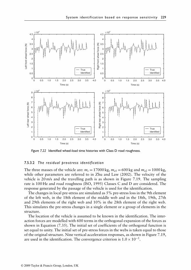
System ident i f i ca t ion based on response sens i t i v i ty 229
0 0.5 1.0 1.5 2.0 2.5 3.0 3.5 4.00
0.5
1
1.5
2
2.5
3
3.5
4
4.5
0
0.5
1
1.5
2
2.5
3
3.5
4
4.5�104
�104
�104�104
Time (s)
0 0.5 1.0 1.5 2.0 2.5 3.0 3.5 4.0
Time (s)
0 0.5 1.0 1.5 2.0 2.5 3.0 3.5 4.0
Time (s)
0 0.5 1.0 1.5 2.0 2.5 3.0 3.5 4.0
Time (s)
Left
fron
t whe
el fo
rce
(N)
TrueIdentified
TrueIdentified
TrueIdentified
TrueIdentified
Rig
ht fr
ont w
heel
forc
e (N
)
0
1
2
3
4
5
6
7
8
9
Left
rear
whe
el fo
rce
(N)
0
1
2
3
4
5
6
7
8
9
Rig
ht r
ear
whe
el fo
rce
(N)
Figure 7.22 Identified wheel-load time histories with Class D road roughness.
7.5.3.2 The res idua l pre-s t ress ident i f i cat ion
The three masses of the vehicle are: mc = 17000 kg, ma1 = 600 kg and ma2 = 1000 kg,while other parameters are referred to in Zhu and Law (2002). The velocity of thevehicle is 20 m/s and the travelling path is as shown in Figure 7.19. The samplingrate is 100 Hz and road roughness (ISO, 1995) Classes C and D are considered. Theresponse generated by the passage of the vehicle is used for the identification.
The changes in local pre-stress are simulated as 5% pre-stress loss in the 9th elementof the left web, in the 18th element of the middle web and in the 18th, 19th, 27thand 29th elements of the right web and 10% in the 28th element of the right web.This simulates the pre-stress changes in a single element or a group of elements in thestructure.
The location of the vehicle is assumed to be known in the identification. The inter-action forces are modelled with 600 terms in the orthogonal expansion of the forces asshown in Equation (7.35). The initial set of coefficients of the orthogonal function isset equal to unity. The initial set of pre-stress forces in the webs is taken equal to thoseof the original structure. Nine vertical acceleration responses, as shown in Figure 7.19,are used in the identification. The convergence criterion is 1.0 × 10⁻⁵.
© 2009 Taylor & Francis Group, London, UK
230 Damage mode ls and a lgor i thms
Table 7.4 Errors in the identified results.
Identified forces or Error (%)residual pre-stress
Class C Class D
Left web 9th 1.20 × 10⁻⁷ 9.95 × 10⁻⁷
Middle web 18th 3.86 × 10⁻⁸ 2.49 × 10⁻⁷
18th 1.74 × 10⁻⁷ 2.41 × 10⁻⁷
19th 4.42 × 10⁻⁷ 5.50 × 10⁻⁷
27th 6.15 × 10⁻⁷ 1.27 × 10⁻⁶
Right web 28th 1.26 × 10⁻⁷ 2.07 × 10⁻⁶
29th 5.61 × 10⁻⁷ 3.71 × 10⁻⁶
Left front wheel load 9.77 × 10⁻⁹ 3.34 × 10⁻⁸
Right front wheel load 7.27 × 10⁻⁹ 3.29 × 10⁻⁸
Left rear wheel load 9.43 × 10⁻⁹ 1.99 × 10⁻⁸
Right rear wheel load 5.50 × 10⁻⁹ 1.45 × 10⁻⁸
Table 7.5 Information at convergence of results.
Class C Class D
Required iterations 5 4Error of convergence 8.48 × 10⁻⁸ 3.39 × 10⁻⁶
Regularization parameter λ 1.9103 × 10⁻¹⁴ 3.0366 × 10⁻¹⁵
There are 375 time instances with the vehicle on the bridge deck, and hence thereare 9 × 375 = 3375 simultaneous equations in Equation (7.36), which is larger than4 × 600 + 108 = 2508 unknowns in the inverse problem.
Figure 7.22 gives the identified force time histories with Class D road roughnesscompared with the true values. The identified forces are overlapping with the truevalues with very small errors as shown in Table 7.4. The errors in the identified pre-stress of the selected elements are also shown in Table 7.4 while those in the unselectedelements are close to zero. Table 7.5 gives the associated information for convergence.The method is shown to be able to effectively identify the interaction forces and localpre-stress change simultaneously in a large complex bridge structure.
7.6 Conclusions
The response sensitivity approach leads to analytical relationships between the dynamicresponse and the system parameters, including the excitation force. Different featuresof system identification using this approach could be performed with these analyticalrelationships as illustrated in this chapter. Developments described in this chapterlead to further development of another time response approach based on wavelets asdiscussed in the next chapter.
© 2009 Taylor & Francis Group, London, UK
Chapter 8
System identification with wavelet
8.1 Introduction
In the last decade, wavelet theory has been one of the emerging and fast-evolving math-ematical and signal processing tools for vibration analysis. Staszewski (1998) presenteda summary of recent advances and applications of wavelet analysis for damage detec-tion. Kijewski and Kareem (2003) studied wavelet transforms for system identificationin civil engineering. The main advantage of the continuous wavelet transform is its abil-ity to provide information simultaneously in time and scale with adaptive windows.Wang and Deng (1999) proposed that the wavelet transform be directly applied tospatially distributed structural response signals, such as surface profile, displacement,strain and acceleration measurements. The continuous wavelet transform of the funda-mental mode shape and its Lipschitz exponent was used to detect the damage locationand extent in a beam (Hong et al., 2002; Chang and Chen, 2003; Douka et al., 2003;Gentile and Messina, 2003). The main purpose of this application is to check thespatially distributed response signals that can pick up damage information.
8.1.1 The wavelets
Many existing vibration-based approaches for damage detection require the modalproperties with the aid of the traditional Fourier transform. There are a few inherentcharacteristics of the Fourier transform that might affect the accuracy of the damageidentification. Firstly, the Fourier transform is a data reduction process and informa-tion on the structural condition might be lost during the process (Sun and Chang,2002a). Secondly, the Fourier transform is a global analysis technique, and its basisfunctions are global functions. Any perturbation of the function at any point in the timedomain influences every point in the frequency domain. This means that the Fouriertransform does not exhibit the time dependency of signals and it cannot capture theevolutionary characteristics that are commonly observed in the measured signals fromstructures under random excitation (Gurley and Kareem, 1999). Damage is typicallya local phenomenon which tends to be captured in high frequency modes. These highfrequencies are normally closely spaced but poorly excited. All these factors add diffi-culty to the implementation of Fourier-transform-based damage detection techniques(Sun and Chang, 2002a).
© 2009 Taylor & Francis Group, London, UK
232 Damage mode ls and a lgor i thms
There has been increasing interest in the wavelet-based approach in recent years dueto its success in several applications. The wavelet transform decomposes a signal usingshort duration waves, allowing a refined decomposition, rather than decompositionwith infinite duration sinusoids as with Fourier transforms. The short duration wave,known as the wavelet basis, has a higher energy density than the sinusoid in Fouriertransforms in general. Therefore, in many cases, the wavelets require fewer coefficientsthan Fourier transforms to describe a signal. The wavelet transform is a two-parametertransform. For the time signal, the two domains of the wavelet transform are time, t,and scale, a. The scale, a, can be approximately related to the frequency, ω. The mainadvantage gained by using wavelets in signal analysis is the ability to perform localanalysis of a signal, i.e. to zoom in on any interval of time or space. Wavelet analysisis thus capable of revealing some hidden aspects of the data that other signal analysistechniques fail to detect. This property is particularly important for damage detectionapplications. The wavelet transform is becoming a promising technique for the damageidentification of structures (Staszewski, 1998). A brief background to wavelet analysisis given below.
The continuous wavelet transform of a signal f (t) is defined as
Wf (a, b) = 1√a
∫ +∞
−∞f (t)ψ∗
(t − b
a
)dt (8.1)
where a and b are the dilation and translation parameters, respectively, and ψ(t) isthe mother wavelet. Both a and b are real numbers and a must be positive; ψ∗(t)indicates its complex conjugate. It should be noted that a wavelet family associatedwith a mother wavelet, ψ(t), is generated by two operations: dilation and translation.The translation parameter, b, indicates the location of the moving wavelet windowin the wavelet transform. Shifting the wavelet window along the time axis impliesexamining the signal in the neighbourhood of the current window location. Therefore,information in the time domain remains, in contrast with the Fourier transform wherethe time domain information becomes invisible after the integration over the entiretime domain. The dilation parameter, a, indicates the width of the wavelet window.A small value of a implies a higher-resolution filter, i.e. the signal is examined througha narrow wavelet window in a smaller scale.
The signal f (t) may be recovered or reconstructed by an inverse wavelet transformof Wf (a, b) defined as
f (t) = 1Cψ
∫ +∞
−∞
∫ +∞
−∞(Wf )(a, b)ψ
(t − b
a
)1a2
da db (8.2)
where Cψ is defined as following with the mother wavelet satisfying the admissibilitycondition to ensure the existence of the inverse wavelet transform.
Cψ =∫ +∞
−∞|ψ(ω)|2
|ω| dω < +∞ (8.3)
© 2009 Taylor & Francis Group, London, UK
System ident i f i ca t ion wi th wave let 233
The existence of the integral in Equation (8.3) requires that
�(0) = 0, i.e.∫ +∞
−∞ψ(x)dx = 0 (8.4)
In practical signal processing, a discrete version of the wavelet transform is oftenemployed by discretizing the dilation parameter a and the translation parameter b. Ingeneral, the procedure becomes much more efficient if dyadic values of a and b areused, i.e.
a = 2j b = 2jk j, k ∈ Z (8.5)
where Z is a set of positive integers. For a special choice of ψ(t), the correspondingdiscretized wavelets {ψj,k} are defined as
ψj,k(t) = 2−j/2ψ(2−jt − k) j, k ∈ Z (8.6)
constitute an orthonormal basis for L2(R). Using the orthogonal basis, the waveletexpansion of a function f (t) and the coefficients of the wavelet expansion are defined as
f (t) =∑j,k
dj,kψj,k(t) (8.7)
and
dj,k =∫ +∞
−∞f (t)ψ∗
j,k(t)dt (8.8)
In the discrete wavelet analysis, a signal can be represented by its approximations anddetails. The detail Dj and the approximation Aj at level j are defined as
Dj =∑k∈Z
αj,kψj,k(t), AJ =∑j>J
Dj (8.9)
8.1.2 The wavelet packets
A possible drawback of the wavelet transform is that the frequency resolution is quitepoor in the high frequency region. Hence, there are difficulties when discriminatingsignals containing high frequency components. The wavelet packet transform is anextension of the wavelet transform that provides complete level-by-level decomposi-tion. The wavelet packets are alternative bases formed by linear combinations of theusual wavelet functions (Coifman and Wickerhauser, 1992). As a result, the waveletpacket transform enables the extraction of features from signals containing stationaryand non-stationary components with arbitrary time-frequency resolution. See Sun andChang, 2002a, on the use of wavelet packet signature to detect damage.
Wavelet packets inherit properties such as orthonormality and time-frequency local-ization from their corresponding wavelet functions. A wavelet packet ψi
j,k(t) is a
© 2009 Taylor & Francis Group, London, UK
234 Damage mode ls and a lgor i thms
function with three indices where integers i, j and k are the modulation, scale andtranslation parameters, respectively,
ψij,k(t) = 2j/2ψi(2jt − k), i = 1, 2, 3, . . . (8.10)
The wavelet packet decomposition (WPD) of a time-domain signal f (t) can be cal-culated using a recursive filter-decimation operation (Coifman and Wickerhauser,1992).
The wavelet functions ψij,k(t) can be obtained from the following recursive relation-
ships:
ψ2j(t) = √2
∞∑k=−∞
h(k)ψi(2t − k) (8.11)
ψ2j+1(t) = √2
∞∑k=−∞
g(k)ψi(2t − k) (8.12)
The first two wavelets are the usual scaling function φ(t) and the mother waveletfunction ψ(t), where
ψ0(t) = φ(t), ψ1(t) = ψ(t) (8.13)
The discrete filters h(k) and g(k) are the quadrature mirror filters associated with thescaling function and the mother wavelet function. Most of the existing mother waveletsare developed to satisfy essential properties such as the invertibility and orthogonality.
The Wavelet Transform (WT) consists of one high frequency term from each leveland one low-frequency residual from the last level of decomposition. The WaveletPacket Transform (WPT), however, contains a complete decomposition at every leveland hence can achieve a higher resolution in the high frequency region. The recursiverelations between the jth and the (j + 1)th level components are
f ij (t) = f 2i−1
j+1 (t) + f 2ij+1(t), (8.14)
f 2i−1j+1 (t) = Hf i
j (t), (8.15)
f 2ij+1(t) = Gf i
j (t), (8.16)
where H and G are the filtering–decimation operators related to the discrete filtersh(k) and g(k) in such a way that
H{·} =∞∑
k=−∞h(k − 2t), (8.17)
G{·} =∞∑
k=−∞g(k − 2t), (8.18)
© 2009 Taylor & Francis Group, London, UK
System ident i f i ca t ion wi th wave let 235
After the j level of decomposition, the original signal f (t) can be expressed as
f (t) =2j∑
i=1
f ij (t) (8.19)
The wavelet packet component signal f ij (t) can be represented by a linear combination
of wavelet packet functions, ψij,k(t), as
f ij (t) =
∞∑k=−∞
cij,k(t)ψi
j,k(t), (8.20)
where the wavelet packet coefficients cij,k(t) can be obtained from
cij,k(t) =
∫ ∞
−∞f (t)ψi
j,k(t)dt (8.21)
provided that the wavelet packet functions are orthogonal, i.e.
ψmj,k(t)ψn
j,k = 0 if m = n
Each component in the wavelet packet decomposition can be viewed as the outputof a filter tuned to a particular basis function. At the lower decomposition level, theWPD yields a good resolution in the time domain but a poor resolution in the frequencydomain. While, at the higher decomposition level, the WPD results in a good resolutionin the frequency domain but a poor resolution in the time domain. For the purposeof structural health monitoring, discrete information in the frequency domain is moreimportant and thus a high level of the WPD is often required to detect the minutechanges in the signals.
8.2 Identification of crack in beam under operating load
An early application of wavelet theory in the spatial domain crack identification ofstructures was proposed by Liew and Wang (1998). The wavelet in the spatial domainis calculated based on finite difference solutions of a mathematical representation of thestructure in question. The crack location is indicated by a peak in the variations ofthe wavelets along the length of the beam. A classical measurement system such as theimpulse hammer technique, is only able to measure mode shapes at a few discrete pointsof a transversely vibrating beam. Therefore, new sensors or measuring techniques areneeded to pick up the perturbations caused by the presence of a crack. Recently thepossibility of measuring displacements on denser grids (a few hundred of points) byusing a laser scanning vibrometer was reported (Pai and Young, 2001).
One of the questions that is attracting significant research attention is related tothe use of the structural response from operational dynamic loads in a damage detec-tion procedure. The operational loads for bridges are moving vehicular loads, and theoperational deflection shapes are the deflections of the bridge deck subject to moving
© 2009 Taylor & Francis Group, London, UK
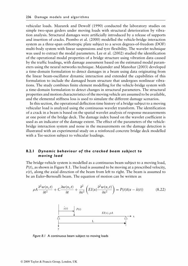
236 Damage mode ls and a lgor i thms
vehicular loads. Mazurek and Dewolf (1990) conducted the laboratory studies onsimple two-span girders under moving loads with structural deterioration by vibra-tion analysis. Structural damages were artificially introduced by a release of supportsand insertion of cracks. Piombo et al. (2000) modelled the vehicle-bridge interactionsystem as a three-span orthotropic plate subject to a seven degrees-of-freedom (DOF)multi-body system with linear suspensions and tyre flexibility. The wavelet techniquewas used to extract the modal parameters. Lee et al. (2002) studied the identificationof the operational modal properties of a bridge structure using vibration data causedby the traffic loadings, with damage assessment based on the estimated modal param-eters using the neural networks technique. Majumder and Manohar (2003) developeda time-domain formulation to detect damages in a beam using data originating fromthe linear beam-oscillator dynamic interaction and extended the capabilities of thisformulation to include the damaged beam structure that undergoes nonlinear vibra-tions. The study combines finite element modelling for the vehicle-bridge system witha time-domain formulation to detect changes in structural parameters. The structuralproperties and motion characteristics of the moving vehicle are assumed to be available,and the elemental stiffness loss is used to simulate the different damage scenarios.
In this section, the operational deflection time history of a bridge subject to a movingvehicular load is analyzed using the continuous wavelet transform. The identificationof a crack in a beam is based on the spatial wavelet analysis of response measurementsat one point of the bridge deck. The damage index based on the wavelet coefficient isused as an indicator of the damage extent. The effect of the parameters of the vehicle-bridge interaction system and noise in the measurements on the damage detection isillustrated with an experimental study on a reinforced concrete bridge deck modelledwith a Tee-section subject to vehicular loadings.
8.2.1 Dynamic behaviour of the cracked beam subject tomoving load
The bridge-vehicle system is modelled as a continuous beam subject to a moving load,P(t), as shown in Figure 8.1. The load is assumed to be moving at a prescribed velocity,v(t), along the axial direction of the beam from left to right. The beam is assumed tobe an Euler–Bernoulli beam. The equation of motion can be written as
ρA∂2w(x, t)∂t2
+ C∂w(x, t)∂t
+ ∂2
∂x2
(EI(x)
∂2w(x, t)∂x2
)= P(t)δ(x − x(t)) (8.22)
x∧(t) P(t)
EI(x), ρA
y
L
x
Figure 8.1 A continuous beam subject to moving loads
© 2009 Taylor & Francis Group, London, UK
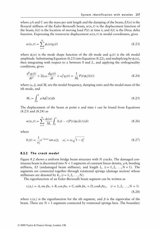
System ident i f i ca t ion wi th wave let 237
where ρA and C are the mass per unit length and the damping of the beam; EI(x) is theflexural stiffness of the Euler–Bernoulli beam; w(x, t) is the displacement function ofthe beam; x(t) is the location of moving load P(t) at time t; and δ(t) is the Dirac deltafunction. Expressing the transverse displacement w(x, t) in modal coordinates, gives
w(x, t) =∞∑
i=1
φi(x)qi(t) (8.23)
where φi(x) is the mode shape function of the ith mode and qi(t) is the ith modalamplitude. Substituting Equation (8.23) into Equation (8.22), and multiplying by φi(x),then integrating with respect to x between 0 and L, and applying the orthogonalityconditions, gives
d2qi(t)dt2
+ 2ξiωidqi(t)
dt+ ω2
i qi(t) = 1Mi
P(t)φi(x(t)) (8.24)
where ωi, ξi and Mi are the modal frequency, damping ratio and the modal mass of theith mode, and
Mi =∫ L
0ρAφ2
i (x)dx (8.25)
The displacement of the beam at point x and time t can be found from Equations(8.23) and (8.24) as
w(x, t) =∞∑
i=1
φi(x)Mi
∫ t
0hi(t − τ)P(τ)φi(x(τ))dτ (8.26)
where
hi(t) = 1ω′
i
e−ξiωi t sinω′it; ω′
i = ωi
√1 − ξ2i (8.27)
8.2.2 The crack model
Figure 8.2 shows a uniform bridge beam structure with N cracks. The damaged con-tinuous beam is discretized into N + 1 segments of constant linear density, ρA; bendingstiffness, EI (undamaged beam stiffness); and length li, (i = 1, 2, . . . , N + 1). Thesegments are connected together through rotational springs (damage section) whosestiffnesses are denoted by ki, (i = 1, 2, . . . , N).
The eigenfunction of an Euler–Bernoulli beam segment can be written as
ri(xi) = Ai sin βxi + Bi cosβxi + Ci sinh βxi + Di cosh βxi, (i = 1, 2, . . . , N + 1)
(8.28)
where ri(xi) is the eigenfunction for the ith segment, and β is the eigenvalue of thebeam. There are N + 1 segments connected by rotational springs here. The boundary
© 2009 Taylor & Francis Group, London, UK
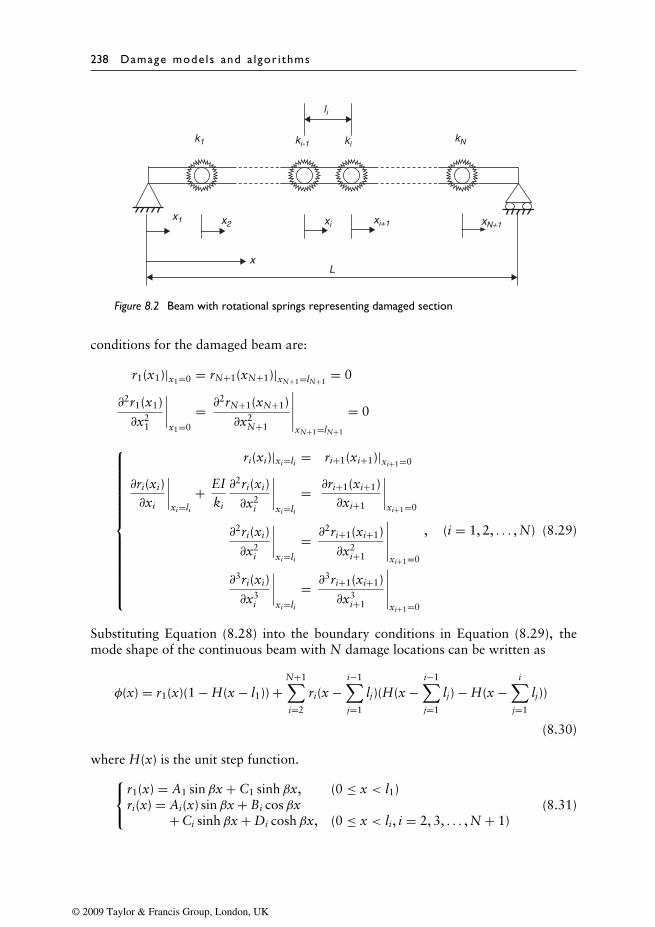
238 Damage mode ls and a lgor i thms
L
xN+1xi+1xix1
k1 ki-1 kikN
x2
li
x
Figure 8.2 Beam with rotational springs representing damaged section
conditions for the damaged beam are:
r1(x1)|x1=0 = rN+1(xN+1)|xN+1=lN+1= 0
∂2r1(x1)
∂x21
∣∣∣∣x1=0
= ∂2rN+1(xN+1)
∂x2N+1
∣∣∣∣∣xN+1=lN+1
= 0
ri(xi)|xi=li = ri+1(xi+1)|xi+1=0
∂ri(xi)∂xi
∣∣∣∣xi=li
+ EIki
∂2ri(xi)
∂x2i
∣∣∣∣xi=li
= ∂ri+1(xi+1)∂xi+1
∣∣∣∣xi+1=0
∂2ri(xi)
∂x2i
∣∣∣∣xi=li
= ∂2ri+1(xi+1)
∂x2i+1
∣∣∣∣∣xi+1=0
∂3ri(xi)
∂x3i
∣∣∣∣xi=li
= ∂3ri+1(xi+1)
∂x3i+1
∣∣∣∣∣xi+1=0
, (i = 1, 2, . . . , N) (8.29)
Substituting Equation (8.28) into the boundary conditions in Equation (8.29), themode shape of the continuous beam with N damage locations can be written as
φ(x) = r1(x)(1 − H(x − l1)) +N+1∑i=2
ri(x −i−1∑j=1
lj)(H(x −i−1∑j=1
lj) − H(x −i∑
j=1
lj))
(8.30)
where H(x) is the unit step function.r1(x) = A1 sin βx + C1 sinh βx, (0 ≤ x < l1)ri(x) = Ai(x) sinβx + Bi cosβx
+ Ci sinh βx + Di cosh βx, (0 ≤ x < li, i = 2, 3, . . . , N + 1)(8.31)
© 2009 Taylor & Francis Group, London, UK
System ident i f i ca t ion wi th wave let 239
and parameters {A} = {β, A1, C1, Ai, Bi, Ci, Di} (i = 2, 3, . . . , N + 1) are determinedfrom the following equation.
[S]{A} = 0 (8.32)
and the elements of matrix S are referred to (Zhu and Law, 2006).
8.2.3 Crack identif ication using continuous wavelet transform
Equation (8.30) shows that there are discontinuities at the damage points, particularlythe slope discontinuities at the cracks. Mode shape curvature is widely used to find thesediscontinuous points (Pandey et al., 1991). However, the first problem for damagedetection using curvature directly is to calculate the curvature by derivation whichis very difficult in practice, and the differentiation of the mode shape will furtheramplify the measurement error. The wavelet transform is used here to measure thelocal regularity of a signal.
The continuous wavelet transform of a square-integrable signal, f (x) , where x istime or space, is defined similar to Equation (8.1) (Mallat and Hwang, 1992)
Wf (u, s) = f (x) ⊗ ψs(x) = 1√s
∫ +∞
−∞f (x)ψ∗
(x − u
s
)dx (8.33)
where ⊗ denotes the convolution of two functions; ψs(x) is the dilation of ψ(x) bythe scale factor s; u is the translation indicating the locality; and ψ∗(x) is the complexconjugate of ψ(x), which is a mother wavelet satisfying the following admissibilitycondition in Equation (8.3). From Equation (8.26), the displacement at xm can bewritten as
w(xm, t) =∞∑
i=1
φi(xm)Mi
∫ t
0hi(t − τ)P(τ)φi(x(τ))dτ (8.34)
The second derivation of the displacement with respect to the position of the movingload can be obtained as
∂2w(xm, t)∂2xl(t)
=∞∑
i=1
φi(xm)Mi
∫ t
0hi(t − τ)P(τ)
∂2φi(x(τ))∂x(τ)2
dτ (8.35)
where ∂2φi( x)/∂ x2 is the second-order derivation of the ith mode, which is the curvature
of the displacement mode shape. The second derivative of the displacement with respectto the load position is shown to include the curvature information of the mode.
Let us take the Gaussian function, θ(x), the wavelet of which can be defined as thesecond derivative of the function
ψ(x) = d2θ(x)dx2
(8.36)
© 2009 Taylor & Francis Group, London, UK
240 Damage mode ls and a lgor i thms
The wavelet, ψ(x), in Equation (8.36) is continuous differentiable and is usuallyreferred to as the Mexican Hat wavelet that has the following explicit expression:
ψ(x) = 2√3σπ−1/4
(x2
σ2− 1
)exp
(−x2
2σ2
)(8.37)
where σ is the standard deviation.The wavelet transform for the displacement w(xm, t) is then expressed by the
following relation (Mallat and Hwang, 1992) when the Mexican Hat wavelet isadopted, as
Ww( x(t), s) = w(xm, t) ⊗ ψs(x(t)) = s2 d2
dx(t)2(w(xm, t) ⊗ θs)(x(t)) (8.38)
Equation (8.38) is the multi-scale differential operator of the second order, and the rela-tion between the second differentiability of w(xm, t) and its wavelet transform decaysat fine scales. The wavelet transform Ww( x(t), s) is proportional to the second deriva-tive of w(xm, t) smoothed by the Gaussian function θs(x). So the wavelet transform canbe used to replace the direct differentiation of the displacement to obtain the curvatureproperties. The damage can be determined using the wavelet transform of the opera-tional displacement time history at one point when the beam structure is subject to theaction of the moving load. A similar formulation can be obtained for accelerations.
8.2.4 Numerical study
A simply supported beam, 50 m long, 1.0 m high and 0.5 m wide (Mahmoud, 2001)is used. The elastic modulus and density of the beam are E = 2.1 × 10¹¹ Pa andρ= 7860 kg/m3, and the moving load is a constant F0 = 10 kN. The first six naturalfrequencies are 0.94, 3.75, 8.44, 15.00, 23.44 and 33.75 Hz. The crack compliance,CC, of a rectangular beam with the crack depth ratio δ is (Sun and Chang, 2002b)
CC = 1k
= 2hEI
(δ
1 − δ)2
[5.93 − 16.69δ+ 37.14δ2 − 35.84δ3 + 13.12δ4] (8.39)
The above beam is used in the simulation, and the damping ratio for all modes is takenequal to 0.02. The crack is at 1/3L from the left-hand-side with a depth ratio of 0.5.White noise is added to the calculated responses of the beam to simulate the pollutedmeasurements, and 1%, 3% and 5% noise levels are studied separately.
w = wcalculated + Ep · Nnoise · σ(wcalculated) (8.40)
where w is the polluted displacement; Ep is the noise level; Nnoise is a standard normaldistribution vector with zero mean value and unit standard deviation; and wcalculated
is the calculated displacement, and σ(wcalculated) are their standard deviations. Thecontinuous wavelet transform on the displacement time history at the mid-span arecalculated with dilation s equal to 1 to 512 in unit increments.
© 2009 Taylor & Francis Group, London, UK
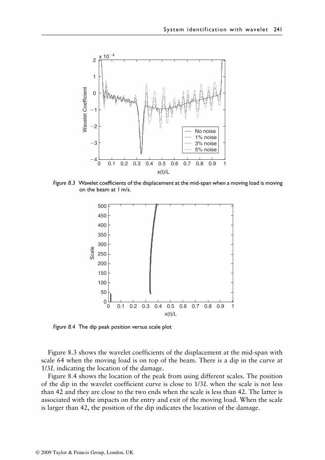
System ident i f i ca t ion wi th wave let 241
0 0.1 0.2 0.3 0.4 0.5 0.6 0.7 0.8 0.9 1�4
�3
�2
�1
0
1
2x 10�4
Wav
elet
Coe
ffici
ent
x(t)/L
No noise1% noise3% noise5% noise
Figure 8.3 Wavelet coefficients of the displacement at the mid-span when a moving load is movingon the beam at 1 m/s.
0 0.1 0.2 0.3 0.4 0.5 0.6 0.7 0.8 0.9 10
50
100
150
200
250
300
350
400
450
500
x(t)/L
Sca
le
Figure 8.4 The dip peak position versus scale plot
Figure 8.3 shows the wavelet coefficients of the displacement at the mid-span withscale 64 when the moving load is on top of the beam. There is a dip in the curve at1/3L indicating the location of the damage.
Figure 8.4 shows the location of the peak from using different scales. The positionof the dip in the wavelet coefficient curve is close to 1/3L when the scale is not lessthan 42 and they are close to the two ends when the scale is less than 42. The latter isassociated with the impacts on the entry and exit of the moving load. When the scaleis larger than 42, the position of the dip indicates the location of the damage.
© 2009 Taylor & Francis Group, London, UK
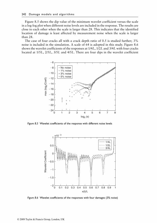
242 Damage mode ls and a lgor i thms
Figure 8.5 shows the dip value of the minimum wavelet coefficient versus the scalein a log-log plot when different noise levels are included in the response. The results areclose to each other when the scale is larger than 28. This indicates that the identifiedlocation of damage is least affected by measurement noise when the scale is largerthan 28.
The case of four cracks all with a crack depth ratio of 0.5 is studied further; 3%noise is included in the simulation. A scale of 64 is adopted in this study. Figure 8.6shows the wavelet coefficients of the responses at 1/4L, 1/2L and 3/4L with four crackslocated at 1/5L, 2/5L, 3/5L and 4/5L. There are four dips in the wavelet coefficient
0 1 2 3 4 5 6 7 8�24
�22
�20
�18
�16
�14
�12
�10
�8
�6
max
(lo
g 2|C
oef|)
log2 (s)
No noise1% noise3% noise5% noise
Figure 8.5 Wavelet coefficients of the response with different noise levels
0 0.1 0.2 0.3 0.4 0.5 0.6 0.7 0.8 0.9 1�2
�1.5
�1
�0.5
0
0.5
1
1/4L1/2L3/4L
x10�3
Wav
elet
Coe
ffici
ent
x(t)/L
Figure 8.6 Wavelet coefficients of the responses with four damages (3% noise)
© 2009 Taylor & Francis Group, London, UK
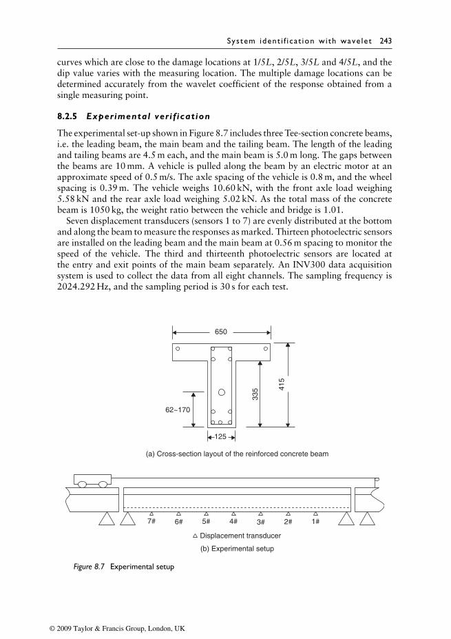
System ident i f i ca t ion wi th wave let 243
curves which are close to the damage locations at 1/5L, 2/5L, 3/5L and 4/5L, and thedip value varies with the measuring location. The multiple damage locations can bedetermined accurately from the wavelet coefficient of the response obtained from asingle measuring point.
8.2.5 Experimental verif ication
The experimental set-up shown in Figure 8.7 includes three Tee-section concrete beams,i.e. the leading beam, the main beam and the tailing beam. The length of the leadingand tailing beams are 4.5 m each, and the main beam is 5.0 m long. The gaps betweenthe beams are 10 mm. A vehicle is pulled along the beam by an electric motor at anapproximate speed of 0.5 m/s. The axle spacing of the vehicle is 0.8 m, and the wheelspacing is 0.39 m. The vehicle weighs 10.60 kN, with the front axle load weighing5.58 kN and the rear axle load weighing 5.02 kN. As the total mass of the concretebeam is 1050 kg, the weight ratio between the vehicle and bridge is 1.01.
Seven displacement transducers (sensors 1 to 7) are evenly distributed at the bottomand along the beam to measure the responses as marked. Thirteen photoelectric sensorsare installed on the leading beam and the main beam at 0.56 m spacing to monitor thespeed of the vehicle. The third and thirteenth photoelectric sensors are located atthe entry and exit points of the main beam separately. An INV300 data acquisitionsystem is used to collect the data from all eight channels. The sampling frequency is2024.292 Hz, and the sampling period is 30 s for each test.
125
7# 6# 5#
Displacement transducer
(b) Experimental setup
4# 3# 2# 1#
(a) Cross-section layout of the reinforced concrete beam
62~170
650
335 41
5
Figure 8.7 Experimental setup
© 2009 Taylor & Francis Group, London, UK
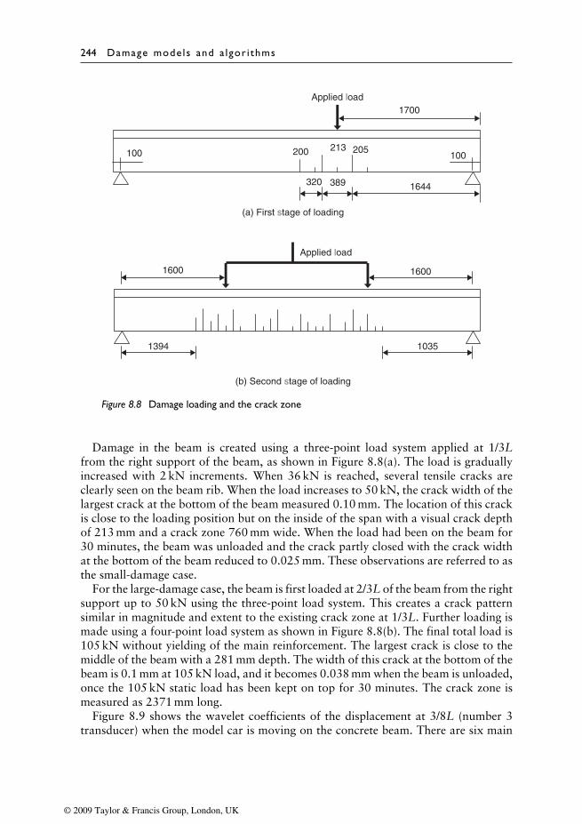
244 Damage mode ls and a lgor i thms
100
1644
1700
320 389
200 213 205100
(a) First stage of loading
1394
1600 1600
1035
(b) Second stage of loading
Applied load
Applied load
Figure 8.8 Damage loading and the crack zone
Damage in the beam is created using a three-point load system applied at 1/3Lfrom the right support of the beam, as shown in Figure 8.8(a). The load is graduallyincreased with 2 kN increments. When 36 kN is reached, several tensile cracks areclearly seen on the beam rib. When the load increases to 50 kN, the crack width of thelargest crack at the bottom of the beam measured 0.10 mm. The location of this crackis close to the loading position but on the inside of the span with a visual crack depthof 213 mm and a crack zone 760 mm wide. When the load had been on the beam for30 minutes, the beam was unloaded and the crack partly closed with the crack widthat the bottom of the beam reduced to 0.025 mm. These observations are referred to asthe small-damage case.
For the large-damage case, the beam is first loaded at 2/3L of the beam from the rightsupport up to 50 kN using the three-point load system. This creates a crack patternsimilar in magnitude and extent to the existing crack zone at 1/3L. Further loading ismade using a four-point load system as shown in Figure 8.8(b). The final total load is105 kN without yielding of the main reinforcement. The largest crack is close to themiddle of the beam with a 281 mm depth. The width of this crack at the bottom of thebeam is 0.1 mm at 105 kN load, and it becomes 0.038 mm when the beam is unloaded,once the 105 kN static load has been kept on top for 30 minutes. The crack zone ismeasured as 2371 mm long.
Figure 8.9 shows the wavelet coefficients of the displacement at 3/8L (number 3transducer) when the model car is moving on the concrete beam. There are six main
© 2009 Taylor & Francis Group, London, UK
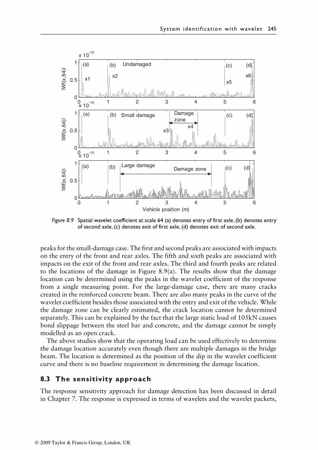
System ident i f i ca t ion wi th wave let 245
0 1 2 3 4 5 60
0.5
1x 10
-10
|Wf(
x,64
)|
0 1 2 3 4 5 60
0.5
1
x 10-10
|Wf(
x,64
)|
0 1 2 3 4 5 60
0.5
1
x 10-10
|Wf(
x,64
)|
Vehicle position (m)
Undamaged
Small damage
Large damage
x1 x2 x6x5
Damagezone
x3x4
Damage zone (a) (b)
(d)(c)
(d)(c)
(b) (a)
(d)(c) (b)(a)
Figure 8.9 Spatial wavelet coefficient at scale 64 (a) denotes entry of first axle, (b) denotes entryof second axle, (c) denotes exit of first axle, (d) denotes exit of second axle.
peaks for the small-damage case. The first and second peaks are associated with impactson the entry of the front and rear axles. The fifth and sixth peaks are associated withimpacts on the exit of the front and rear axles. The third and fourth peaks are relatedto the locations of the damage in Figure 8.9(a). The results show that the damagelocation can be determined using the peaks in the wavelet coefficient of the responsefrom a single measuring point. For the large-damage case, there are many crackscreated in the reinforced concrete beam. There are also many peaks in the curve of thewavelet coefficient besides those associated with the entry and exit of the vehicle. Whilethe damage zone can be clearly estimated, the crack location cannot be determinedseparately. This can be explained by the fact that the large static load of 105kN causesbond slippage between the steel bar and concrete, and the damage cannot be simplymodelled as an open crack.
The above studies show that the operating load can be used effectively to determinethe damage location accurately even though there are multiple damages in the bridgebeam. The location is determined as the position of the dip in the wavelet coefficientcurve and there is no baseline requirement in determining the damage location.
8.3 The sensitivity approach
The response sensitivity approach for damage detection has been discussed in detailin Chapter 7. The response is expressed in terms of wavelets and the wavelet packets,
© 2009 Taylor & Francis Group, London, UK
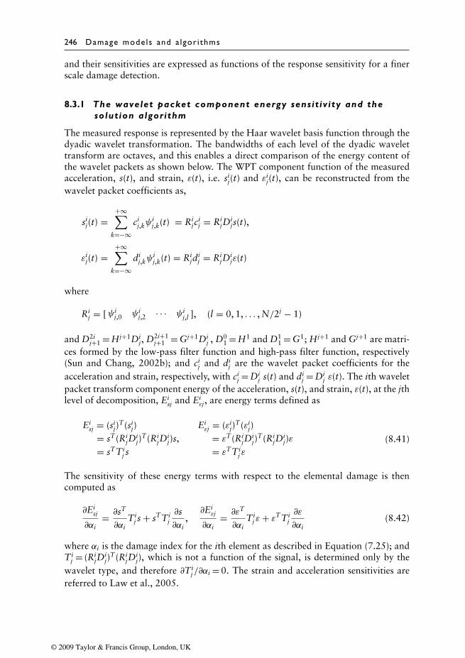
246 Damage mode ls and a lgor i thms
and their sensitivities are expressed as functions of the response sensitivity for a finerscale damage detection.
8.3.1 The wavelet packet component energy sensit iv ity and thesolution algorithm
The measured response is represented by the Haar wavelet basis function through thedyadic wavelet transformation. The bandwidths of each level of the dyadic wavelettransform are octaves, and this enables a direct comparison of the energy content ofthe wavelet packets as shown below. The WPT component function of the measuredacceleration, s(t), and strain, ε(t), i.e. si
j(t) and εij(t), can be reconstructed from thewavelet packet coefficients as,
sij(t) =
+∞∑k=−∞
cij,kψ
ij,k(t) = Ri
jcij = Ri
jDijs(t),
εij(t) =+∞∑
k=−∞di
j,kψij,k(t) = Ri
jdij = Ri
jDijε(t)
where
Rij = [ψi
j,0 ψij,2 · · · ψi
j,l ], (l = 0, 1, . . . , N/2j − 1)
and D2ij+1 = Hj+1Di
j, D2i+1j+1 = Gj+1Di
j , D01 = H1 and D1
1 = G1; Hj+1 and Gj+1 are matri-ces formed by the low-pass filter function and high-pass filter function, respectively(Sun and Chang, 2002b); and ci
j and dij are the wavelet packet coefficients for the
acceleration and strain, respectively, with cij = Di
j s(t) and dij = Di
j ε(t). The ith waveletpacket transform component energy of the acceleration, s(t), and strain, ε(t), at the jthlevel of decomposition, Ei
sj and Eiεj, are energy terms defined as
Eisj = (si
j)T (si
j) Eiεj = (εij)
T (εij)= sT (Ri
jDij)
T (RijD
ij)s, = εT (Ri
jDij)
T (RijD
ij)ε
= sTTij s = εTTi
j ε
(8.41)
The sensitivity of these energy terms with respect to the elemental damage is thencomputed as
∂Eisj
∂αi= ∂s
T
∂αiTi
j s + sTTij∂s∂αi
,∂Eiεj
∂αi= ∂ε
T
∂αiTi
j ε+ εTTij∂ε
∂αi(8.42)
where αi is the damage index for the ith element as described in Equation (7.25); andTi
j = (RijD
ij)
T (RijD
ij), which is not a function of the signal, is determined only by the
wavelet type, and therefore ∂Tij /∂αi = 0. The strain and acceleration sensitivities are
referred to Law et al., 2005.
© 2009 Taylor & Francis Group, London, UK
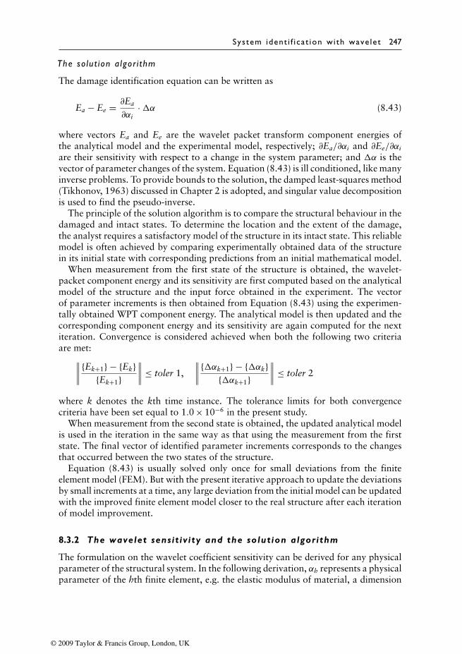
System ident i f i ca t ion wi th wave let 247
The so lut ion a lgor i thm
The damage identification equation can be written as
Ea − Ee = ∂Ea
∂αi·�α (8.43)
where vectors Ea and Ee are the wavelet packet transform component energies ofthe analytical model and the experimental model, respectively; ∂Ea/∂αi and ∂Ee/∂αi
are their sensitivity with respect to a change in the system parameter; and �α is thevector of parameter changes of the system. Equation (8.43) is ill conditioned, like manyinverse problems. To provide bounds to the solution, the damped least-squares method(Tikhonov, 1963) discussed in Chapter 2 is adopted, and singular value decompositionis used to find the pseudo-inverse.
The principle of the solution algorithm is to compare the structural behaviour in thedamaged and intact states. To determine the location and the extent of the damage,the analyst requires a satisfactory model of the structure in its intact state. This reliablemodel is often achieved by comparing experimentally obtained data of the structurein its initial state with corresponding predictions from an initial mathematical model.
When measurement from the first state of the structure is obtained, the wavelet-packet component energy and its sensitivity are first computed based on the analyticalmodel of the structure and the input force obtained in the experiment. The vectorof parameter increments is then obtained from Equation (8.43) using the experimen-tally obtained WPT component energy. The analytical model is then updated and thecorresponding component energy and its sensitivity are again computed for the nextiteration. Convergence is considered achieved when both the following two criteriaare met:∥∥∥∥ {Ek+1} − {Ek}
{Ek+1}∥∥∥∥ ≤ toler 1,
∥∥∥∥ {�αk+1} − {�αk}{�αk+1}
∥∥∥∥ ≤ toler 2
where k denotes the kth time instance. The tolerance limits for both convergencecriteria have been set equal to 1.0 × 10⁻⁶ in the present study.
When measurement from the second state is obtained, the updated analytical modelis used in the iteration in the same way as that using the measurement from the firststate. The final vector of identified parameter increments corresponds to the changesthat occurred between the two states of the structure.
Equation (8.43) is usually solved only once for small deviations from the finiteelement model (FEM). But with the present iterative approach to update the deviationsby small increments at a time, any large deviation from the initial model can be updatedwith the improved finite element model closer to the real structure after each iterationof model improvement.
8.3.2 The wavelet sensit iv ity and the solution algorithm
The formulation on the wavelet coefficient sensitivity can be derived for any physicalparameter of the structural system. In the following derivation, αh represents a physicalparameter of the hth finite element, e.g. the elastic modulus of material, a dimension
© 2009 Taylor & Francis Group, London, UK

248 Damage mode ls and a lgor i thms
or the second moment of inertia of a cross-section. Both analytical and computationalapproaches to obtain the sensitivity of the wavelet coefficient are given below.
Analy t i ca l approach
Expressing the responses z,•z and
••z in terms of the wavelet transforms and substituting
into the equation of motion of the structural system, gives
M
∑j,k
d1j,k
••ψj,k(t)∑
j,kd2
j,k
••ψj,k(t)
· · ·∑j,k
dNj,k
••ψj,k(t)
+ C
∑j,k
d1j,k
•ψj,k(t)∑
j,kd2
j,k
•ψj,k(t)
· · ·∑j,k
dNj,k
•ψj,k(t)
+ K
∑j,k
d1j,kψj,k(t)∑
j,kd2
j,kψj,k(t)
· · ·∑j,k
dNj,kψj,k(t)
= D
∑j,k
dFj,kψj,k(t)
(8.44)
where M, C and K are the mass, damping, stiffness matrices, respectively; z,•z and
••z are the displacement, velocity and acceleration vectors, respectively; D is the map-ping matrix relating the force vector F(t) to the corresponding DOFs of the system;and dF
j,k = ∫R F(t)ψj,k(t)dt. Computing the inner product with ψj,k(t) on both sides of
Equation (8.44), and noting the orthogonal property of the wavelets, gives
(M∫ ••ψj,k(t)ψj,k(t)dt + C
∫ •ψj,k(t)ψj,k(t)dt + K
)d1
j,kd2
j,k· · ·dN
j,k
= DdFj,k (8.45)
Since∫ ••ψj,k(t)ψj,k(t)dt and
∫ •ψj,k(t)ψj,k(t)dt are functions of the wavelets only, they can
be expressed as
aj,k =∫ ••ψj,k(t)ψj,k(t)dt, bj,k =
∫ •ψj,k(t)ψj,k(t)dt
and Equation (8.45) becomes
(Maj,k + Cbj,k + K){
d1j,k d2
j,k · · · dNj,k
}T = DdFj,k (8.46)
rewriting this gives
{d1
j,k d2j,k · · · dN
j,k
}T = (Maj,k + Cbj,k + K)−1DdFj,k (8.47)
© 2009 Taylor & Francis Group, London, UK

System ident i f i ca t ion wi th wave let 249
Differentiating both sides of Equation (8.46) with respect to the damage index, αh, gives
(∂M∂αh
aj,k + ∂C∂αh
bj,k + ∂K∂αh
)d1
j,k
d2j,k
· · ·dN
j,k
+ (Maj,k + Cbj,k + K)
∂d1j,k
∂αh
∂d2j,k
∂αh· · ·∂dN
j,k
∂αh
= 0 (8.48)
Substituting Equation (8.47) into (8.48), finally gives the wavelet coefficient sensitivityin terms of the system parameter as{
∂d1j,k
∂αh
∂d2j,k
∂αh· · · ∂dN
j,k
∂αh
}T
= −(Maj,k + Cbj,k + K)−1
×(∂M∂αh
aj,k + ∂C∂αh
bj,k + ∂K∂αh
)(Maj,k + Cbj,k + K)−1DdF
j,k (8.49)
Computat iona l approach
Differentiating the formulation of the wavelet coefficient in Equation (8.8) with respectto αh, gives
∂dj,k
∂αh= ∂
∂αh
∫R
f (t)ψj,k(t)dt
(8.50a)
Since ψj,k(t) is not related to αh, we have
∂dj,k
∂αh=∫R
∂f (t)∂αhψj,k(t)dt (8.50b)
where ∂f (t)/∂αh is the sensitivity of response to a local change in αh.Equation (8.50) can also be obtained in an alternative formulation. Express the
response sensitivity ∂f (t)/∂αh in terms of wavelets, and the wavelet coefficient, cj,k, isobtained as
cj,k =∫R
∂f (t)∂αhψj,k(t)dt (8.51)
Comparing Equations (8.50) and (8.51), gives
∂dj,k
∂αh= cj,k (8.52)
© 2009 Taylor & Francis Group, London, UK
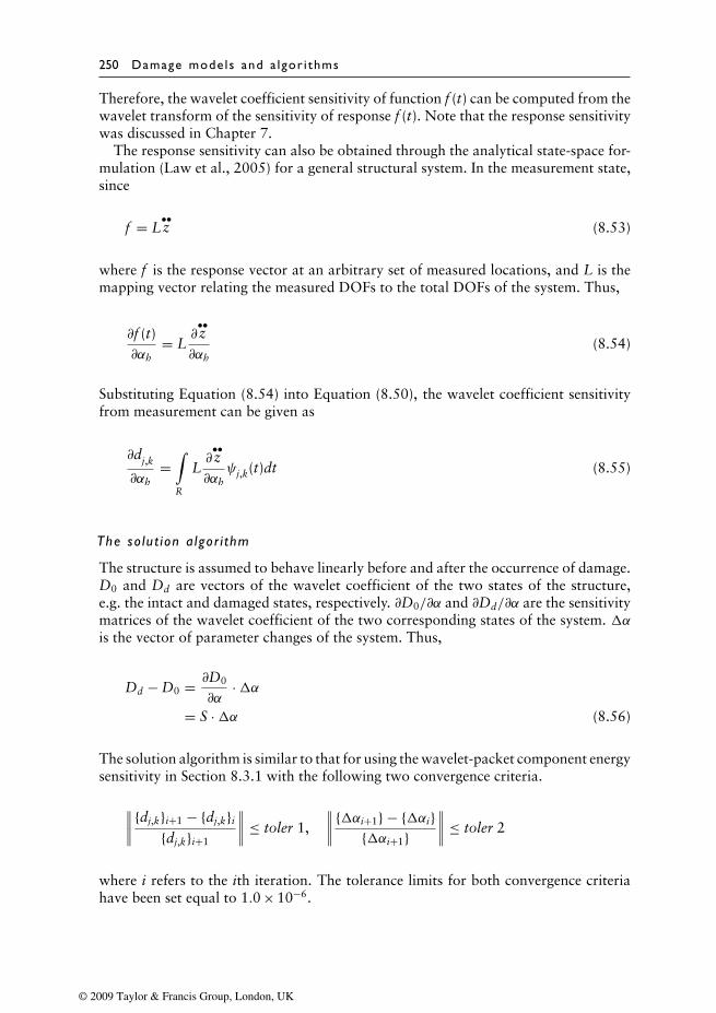
250 Damage mode ls and a lgor i thms
Therefore, the wavelet coefficient sensitivity of function f (t) can be computed from thewavelet transform of the sensitivity of response f (t). Note that the response sensitivitywas discussed in Chapter 7.
The response sensitivity can also be obtained through the analytical state-space for-mulation (Law et al., 2005) for a general structural system. In the measurement state,since
f = L••z (8.53)
where f is the response vector at an arbitrary set of measured locations, and L is themapping vector relating the measured DOFs to the total DOFs of the system. Thus,
∂f (t)∂αh
= L∂
••z
∂αh(8.54)
Substituting Equation (8.54) into Equation (8.50), the wavelet coefficient sensitivityfrom measurement can be given as
∂dj,k
∂αh=∫R
L∂
••z
∂αhψj,k(t)dt (8.55)
The so lut ion a lgor i thm
The structure is assumed to behave linearly before and after the occurrence of damage.D0 and Dd are vectors of the wavelet coefficient of the two states of the structure,e.g. the intact and damaged states, respectively. ∂D0/∂α and ∂Dd/∂α are the sensitivitymatrices of the wavelet coefficient of the two corresponding states of the system. �αis the vector of parameter changes of the system. Thus,
Dd − D0 = ∂D0
∂α·�α
= S ·�α (8.56)
The solution algorithm is similar to that for using the wavelet-packet component energysensitivity in Section 8.3.1 with the following two convergence criteria.
∥∥∥∥ {dj,k}i+1 − {dj,k}i
{dj,k}i+1
∥∥∥∥ ≤ toler 1,∥∥∥∥ {�αi+1} − {�αi}
{�αi+1}∥∥∥∥ ≤ toler 2
where i refers to the ith iteration. The tolerance limits for both convergence criteriahave been set equal to 1.0 × 10⁻⁶.
© 2009 Taylor & Francis Group, London, UK
System ident i f i ca t ion wi th wave let 251
8.3.3 The wavelet packet transform sensit iv ity
The wavelet packet transform was discussed in Section 8.1.2. Assuming that f (t) isthe signal to be transformed, the discrete wavelet packet transform (WPT) coefficients(Mallat and Hwang, 1992) of the signal can be obtained as
cij,k =
∫ +∞
−∞f (t)ψi
j,k(t)dt (8.21)
where i, j and k are the wavelet packet number, the decomposition level and thetranslation respectively (Daubechies, 1988; 1992), and ψi
j,k(t) satisfies the followingrelation
ψij,k(t) = 2− j
2ψi(2−jt − k) (8.10)
where ψi(t) is the ith wavelet packet with the following properties
ψ2i(t) = √2
+∞∑k=−∞
h(k)ψi(2t − k) (8.11)
ψ2i+1(t) = √2
+∞∑k=−∞
g(k)ψi(2t − k), i = 0, 1, . . . , 2j − 1 (8.12)
where h(k) and g(k) are the low-pass and high-pass analysis filters. It is noted that ψ00,k
can be defined as
ψ00,k = ψ0(t − k) = ϕ(t − k) (8.57)
where ϕ(t) is the scale function of the wavelet.The original signal can also be reconstructed from the WPT coefficients as
f (t) =2j−1∑i=0
f ij (t), and f i
j (t) =+∞∑
k=−∞ci
j,kψij,k(t) (8.58)
where f ij (t) denotes the signal component in the ith frequency band.
The WPT is applied to ∂••xl/∂αi and
••xl separately, where ldenotes the lth DOF
of the structure. The relation between WPT(∂••xl/∂αi) and WPT(
••xl) was given in
Section 8.3.2 as
WPT
(∂
••xl
∂αi
)= ∂
∂αiWPT(
••xl) (8.59)
© 2009 Taylor & Francis Group, London, UK
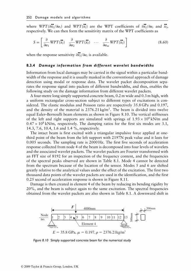
252 Damage mode ls and a lgor i thms
where WPT(∂••xl/∂αi) and WPT(
••xl) are the WPT coefficients of ∂
••xl/∂αi and
••xl,
respectively. We can then form the sensitivity matrix of the WPT coefficients as
S =[∂
∂α1WPT(
••xl)
∂
∂α2WPT(
••xl) · · · ∂
∂αmWPT(
••xl)
](8.60)
when the response sensitivity ∂••xl/∂αi is available.
8.3.4 Damage information from different wavelet bandwidths
Information from local damages may be carried in the signal within a particular band-width of the response and it is usually masked in the conventional approach of damagedetection using modal or response data. The wavelet packet decomposition sepa-rates the response signal into packets of different bandwidths, and thus, enables thefollowing study on the damage information from different wavelet packets.
A four-metre long simply supported concrete beam, 0.2 m wide and 0.3 m high, witha uniform rectangular cross-section subject to different types of excitations is con-sidered. The elastic modulus and Poisson ratio are respectively 35.8 GPa and 0.197,and the density of the material is 2376.21 kg/m3. The beam is divided into twelveequal Euler–Bernoulli beam elements as shown in Figure 8.10. The vertical stiffnessesof the left and right supports are simulated with springs of 1.93 × 10⁸ kN/m and0.47 × 108 kN/m, respectively. The damping ratios for the first six modes are 3.1,14.3, 7.6, 10.4, 1.6 and 1.4 %, respectively.
The intact beam is first excited with a triangular impulsive force applied at one-third point of the beam from the left support with 2197N peak value and it lasts for0.005 seconds. The sampling rate is 2000 Hz. The first five seconds of accelerationresponse collected from node 4 of the beam is decomposed into four levels of waveletsand the associated wavelet packets. The wavelet packets are Fourier transformed withan FFT size of 8192 for an inspection of the frequency content, and the frequenciesof the spectral peaks observed are shown in Table 8.1. Mode 4 cannot be detectedfrom the spectrum because of the location of the sensor. Modes 5 and 6 are shiftedgreatly relative to the analytical values under the effect of the excitation. The first twothousand data points of the wavelet packets are used in the identification, and the first0.25 second of acceleration response is shown in Figure 8.11.
Damage is then created in element 4 of the beam by reducing its bending rigidity by20%, and the beam is subject again to the same excitation. The spectral frequenciesobtained from the wavelet packets are also shown in Table 8.1. A downward shift in
-------- 1 2 3 4 5 6 7 8 9 10 11 12 13
200mm
300m
m
E � 35.8 GPa, m � 0.197, 3r � 2376.21kg/m
4000mmF
Node no.
Element 4
Figure 8.10 Simply supported concrete beam for the numerical study
© 2009 Taylor & Francis Group, London, UK
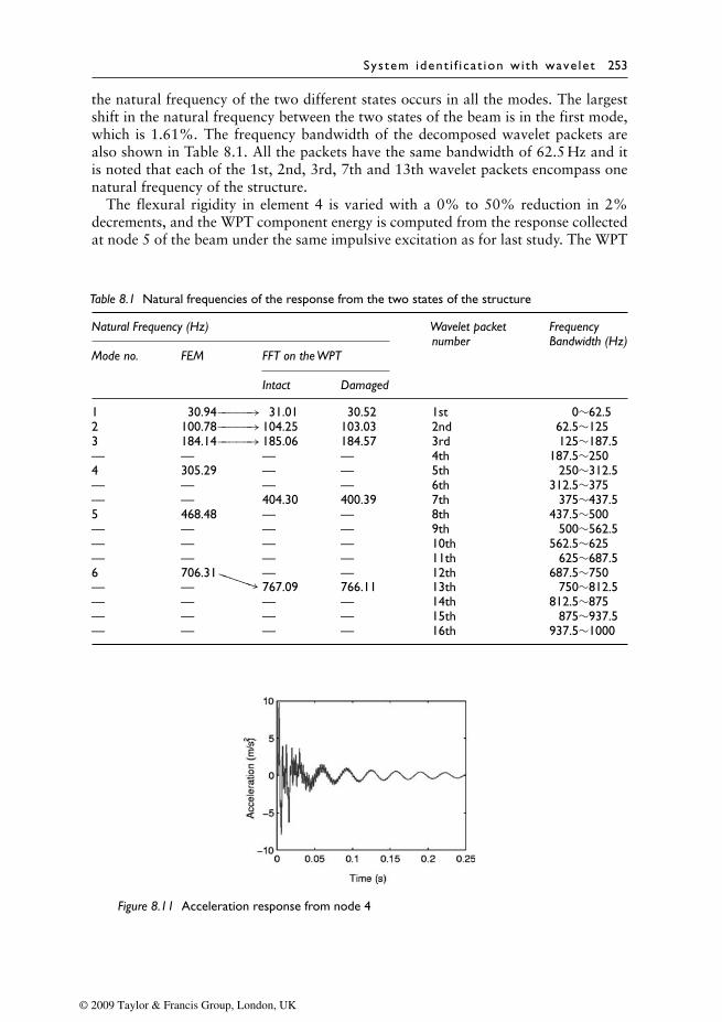
System ident i f i ca t ion wi th wave let 253
the natural frequency of the two different states occurs in all the modes. The largestshift in the natural frequency between the two states of the beam is in the first mode,which is 1.61%. The frequency bandwidth of the decomposed wavelet packets arealso shown in Table 8.1. All the packets have the same bandwidth of 62.5 Hz and itis noted that each of the 1st, 2nd, 3rd, 7th and 13th wavelet packets encompass onenatural frequency of the structure.
The flexural rigidity in element 4 is varied with a 0% to 50% reduction in 2%decrements, and the WPT component energy is computed from the response collectedat node 5 of the beam under the same impulsive excitation as for last study. The WPT
Table 8.1 Natural frequencies of the response from the two states of the structure
Natural Frequency (Hz) Wavelet packet Frequencynumber Bandwidth (Hz)
Mode no. FEM FFT on theWPT
Intact Damaged
1 30.94−−−−−→ 31.01 30.52 1st 0∼62.52 100.78−−−−−→104.25 103.03 2nd 62.5∼1253 184.14−−−−−→185.06 184.57 3rd 125∼187.5— — — — 4th 187.5∼2504 305.29 — — 5th 250∼312.5— — — — 6th 312.5∼375— — 404.30 400.39 7th 375∼437.55 468.48 — — 8th 437.5∼500— — — — 9th 500∼562.5— — — — 10th 562.5∼625— — — — 11th 625∼687.56 706.31−−−−−→ — — 12th 687.5∼750— — 767.09 766.11 13th 750∼812.5— — — — 14th 812.5∼875— — — — 15th 875∼937.5— — — — 16th 937.5∼1000
Figure 8.11 Acceleration response from node 4
© 2009 Taylor & Francis Group, London, UK
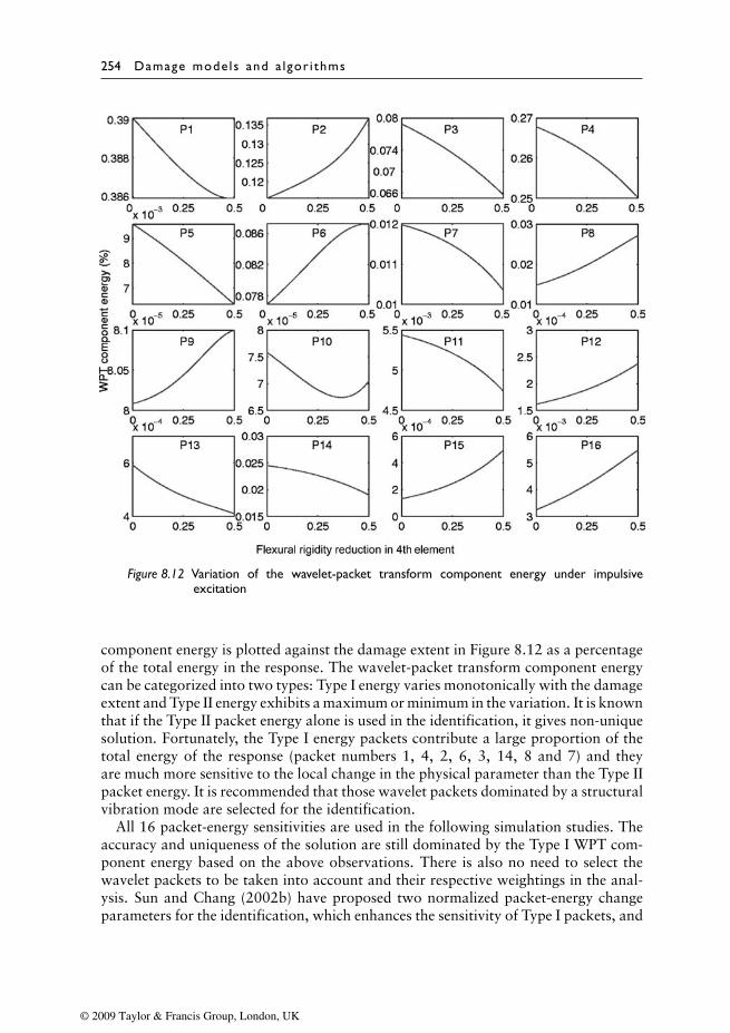
254 Damage mode ls and a lgor i thms
Figure 8.12 Variation of the wavelet-packet transform component energy under impulsiveexcitation
component energy is plotted against the damage extent in Figure 8.12 as a percentageof the total energy in the response. The wavelet-packet transform component energycan be categorized into two types: Type I energy varies monotonically with the damageextent and Type II energy exhibits a maximum or minimum in the variation. It is knownthat if the Type II packet energy alone is used in the identification, it gives non-uniquesolution. Fortunately, the Type I energy packets contribute a large proportion of thetotal energy of the response (packet numbers 1, 4, 2, 6, 3, 14, 8 and 7) and theyare much more sensitive to the local change in the physical parameter than the Type IIpacket energy. It is recommended that those wavelet packets dominated by a structuralvibration mode are selected for the identification.
All 16 packet-energy sensitivities are used in the following simulation studies. Theaccuracy and uniqueness of the solution are still dominated by the Type I WPT com-ponent energy based on the above observations. There is also no need to select thewavelet packets to be taken into account and their respective weightings in the anal-ysis. Sun and Chang (2002b) have proposed two normalized packet-energy changeparameters for the identification, which enhances the sensitivity of Type I packets, and
© 2009 Taylor & Francis Group, London, UK

System ident i f i ca t ion wi th wave let 255
Table 8.2 Damage scenarios
Damage Damage Damage locations Response type Excitation typeScenario extent
1 10% 11th element acceleration Impulsive excitation at node 52 10% 11th element strain3 10% 11th element acceleration and
strain4 5%,10% 6th, 7th element acceleration5 5%,10% 6th, 7th element strain6 5%,10% 6th, 7th element acceleration and
strain7 5%,10%,15% 3rd, 4th, 8th element acceleration8 5%,10%,15% 3rd, 4th, 8th element strain9 5%,10%,15% 3rd, 4th, 8th element acceleration and
strain10 5%,10% 6th, 7th element acceleration Sinusoidal excitation at node 511 5%,10% 6th, 7th element strain12 5%,10% 6th, 7th element acceleration and
and strain13 10% 2nd element acceleration with Impulsive excitation at node 4
5% noise14 5%, 10% 6th, 7th element15(a) 5%, 10% 6th, 7th element Impulsive excitation at node 4
with −3% model error in allelements
15(b) 5%, 10% 6th, 7th element
this will improve the final identified results from the above discussions. Also, a schemefor optimizing the best packets is needed.
Damage scenar ios and the i r detect ion
Twelve damage scenarios were studied with different damage extents and from differenttypes of response, as listed in Table 8.2. In fact, three patterns of damage (singledamage, two adjacent damages and three damages) were considered and each damagepattern was identified from acceleration, strain and both types of response. The firstnine scenarios were studied using the vertical response from node 7 when the beam issubject to the same impulsive excitation at one-third span as for last study. The resultsshown in Figure 8.13 show that either acceleration along or both acceleration andstrain responses together can identify the damage accurately with a very small error.The bad results in Scenario 8 were also noticed. This gives numerical evidence that thestrain response is less sensitive to local damage as observed in its formulation in Lawet al., 2005.
Damage scenarios 10 to 12 were studied using the vertical measured responses fromnodes 7 and 8 when the beam is subject to a sinusoidal excitation at one-third span atthe frequency of 30 Hz close to the fundamental frequency of the beam. The magnitudeof the force is 20N. Results in Figure 8.13 show that this arrangement could identify
© 2009 Taylor & Francis Group, London, UK
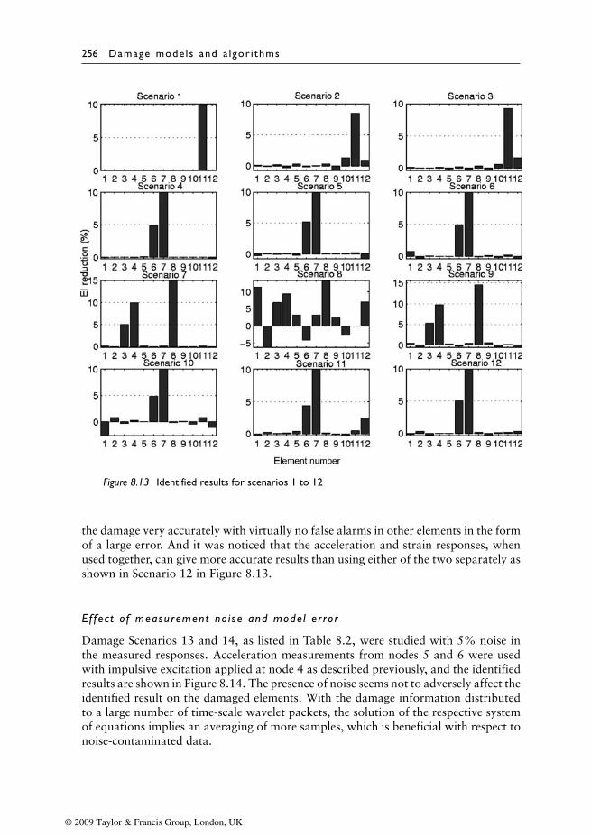
256 Damage mode ls and a lgor i thms
Figure 8.13 Identified results for scenarios 1 to 12
the damage very accurately with virtually no false alarms in other elements in the formof a large error. And it was noticed that the acceleration and strain responses, whenused together, can give more accurate results than using either of the two separately asshown in Scenario 12 in Figure 8.13.
Ef fec t o f measurement no i se and mode l er ror
Damage Scenarios 13 and 14, as listed in Table 8.2, were studied with 5% noise inthe measured responses. Acceleration measurements from nodes 5 and 6 were usedwith impulsive excitation applied at node 4 as described previously, and the identifiedresults are shown in Figure 8.14. The presence of noise seems not to adversely affect theidentified result on the damaged elements. With the damage information distributedto a large number of time-scale wavelet packets, the solution of the respective systemof equations implies an averaging of more samples, which is beneficial with respect tonoise-contaminated data.
© 2009 Taylor & Francis Group, London, UK
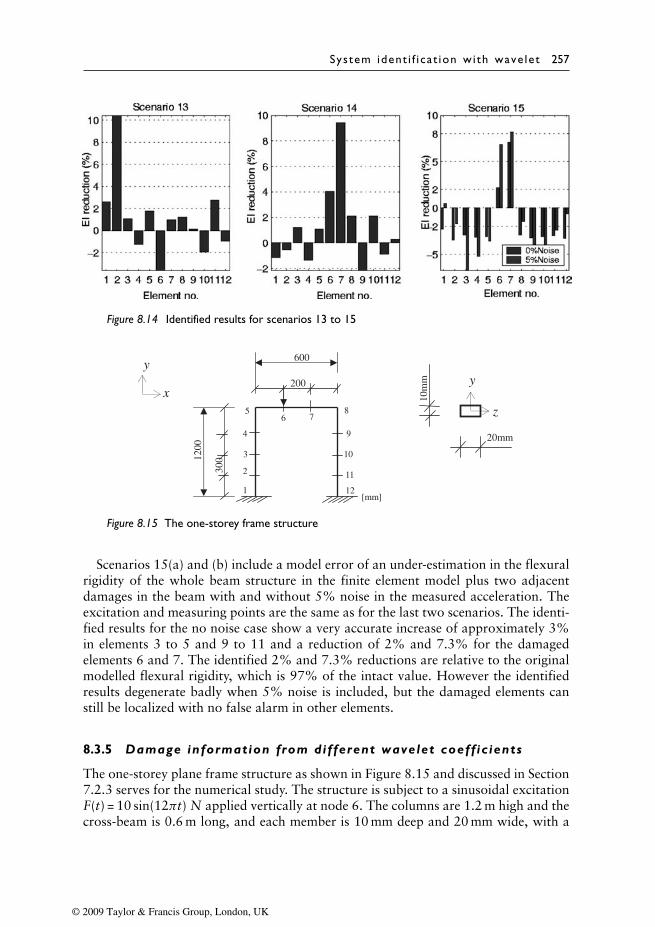
System ident i f i ca t ion wi th wave let 257
Figure 8.14 Identified results for scenarios 13 to 15
1200
10m
m
20mm
y
x
600
200
300
1
3
2
4
5 7 6
8
10
11
9
12 [mm]
y
z
Figure 8.15 The one-storey frame structure
Scenarios 15(a) and (b) include a model error of an under-estimation in the flexuralrigidity of the whole beam structure in the finite element model plus two adjacentdamages in the beam with and without 5% noise in the measured acceleration. Theexcitation and measuring points are the same as for the last two scenarios. The identi-fied results for the no noise case show a very accurate increase of approximately 3%in elements 3 to 5 and 9 to 11 and a reduction of 2% and 7.3% for the damagedelements 6 and 7. The identified 2% and 7.3% reductions are relative to the originalmodelled flexural rigidity, which is 97% of the intact value. However the identifiedresults degenerate badly when 5% noise is included, but the damaged elements canstill be localized with no false alarm in other elements.
8.3.5 Damage information from different wavelet coeff ic ients
The one-storey plane frame structure as shown in Figure 8.15 and discussed in Section7.2.3 serves for the numerical study. The structure is subject to a sinusoidal excitationF(t) = 10 sin(12πt) N applied vertically at node 6. The columns are 1.2 m high and thecross-beam is 0.6 m long, and each member is 10 mm deep and 20 mm wide, with a
© 2009 Taylor & Francis Group, London, UK
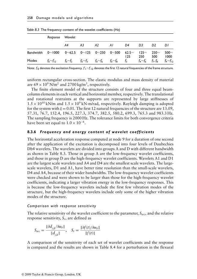
258 Damage mode ls and a lgor i thms
Table 8.3 The frequency content of the wavelet coefficients (Hz)
Response Wavelet
A4 A3 A2 A1 D4 D3 D2 D1
Bandwidth 0∼1000 0∼62.5 0∼125 0∼250 0∼500 62.5∼ 125∼ 250∼ 500∼125 250 500 1000
Modes f0∼f12 f0∼f2 f0∼f3 f0∼f6 f0∼f8 f3 f4∼f6 f7, f8 f9∼f12
Note: f 0 denotes the excitation frequency, f 1∼f 12 denotes the first 12 natural frequencies of the frame structure.
uniform rectangular cross-section. The elastic modulus and mass density of materialare 69 × 109 N/m2 and 2700 kg/m3, respectively.
The finite element model of the structure consists of four and three equal beam-column elements in each vertical and horizontal member, respectively. The translationaland rotational restraints at the supports are represented by large stiffnesses of1.5 × 1010 kN/m and 1.5 × 10⁹ kN-m/rad, respectively. Rayleigh damping is adoptedfor the system with ξ= 0.01. The first 12 natural frequencies of the structure are 13.09,57.31, 76.7, 152.4, 196.5, 227.3, 374.7, 382.5, 580.2, 699.3, 765.3 and 983.3 Hz.The sampling frequency is 2000 Hz. The tolerance limits for both convergence criteriahave been set equal to 1.0 × 10⁻⁶.
8.3.6 Frequency and energy content of wavelet coeff ic ients
The horizontal acceleration response computed at node 9 for a duration of one secondafter the application of the excitation is decomposed into four levels of DaubechiesDb4 wavelets. The wavelets are divided into groups A and D with different bandwidthas shown in Table 8.3. Those in group A are the low-frequency wavelet coefficients,and those in group D are the high-frequency wavelet coefficients. Wavelets A1 and D1are the largest scale wavelets and A4 and D4 are the smallest scale wavelets. The large-scale wavelets, D1 and A1, have better time resolution than the small-scale wavelets,D4 and A4, because of their wider bandwidths. The low-frequency wavelet coefficientswere checked and were shown to be larger than those for the high-frequency waveletcoefficients, indicating a larger vibration energy in the low-frequency responses. Thisis because the low-frequency wavelets include the first few vibration modes of thestructure, but the high-frequency wavelets include only some of the higher vibrationmodes of the structure.
Compar i son wi th response sens i t i v i t y
The relative sensitivity of the wavelet coefficient to the parameter, Swc, and the relativeresponse sensitivity, Sr, are defined as
Swc = ‖∂dj,k/∂αh‖‖dj,k‖
, Sr = ‖∂f (t)/∂αh‖‖f (t)‖
A comparison of the sensitivity of each set of wavelet coefficients and the responseis compared and the results are shown in Table 8.4 for a perturbation in the flexural
© 2009 Taylor & Francis Group, London, UK
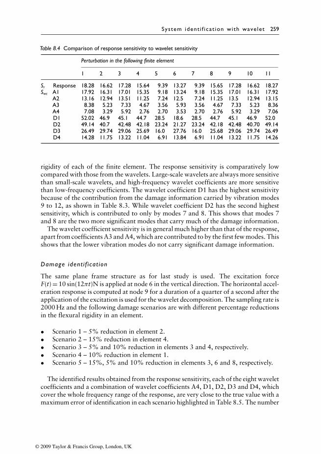
System ident i f i ca t ion wi th wave let 259
Table 8.4 Comparison of response sensitivity to wavelet sensitivity
Perturbation in the following finite element
1 2 3 4 5 6 7 8 9 10 11
Sr Response 18.28 16.62 17.28 15.64 9.39 13.27 9.39 15.65 17.28 16.62 18.27Swc A1 17.92 16.31 17.01 15.35 9.18 13.24 9.18 15.35 17.01 16.31 17.92
A2 13.16 12.94 13.51 11.25 7.24 12.5 7.24 11.25 13.5 12.94 13.15A3 8.38 5.23 7.33 4.67 3.56 5.93 3.56 4.67 7.33 5.23 8.36A4 7.08 3.29 5.92 2.76 2.70 3.53 2.70 2.76 5.92 3.29 7.06D1 52.02 46.9 45.1 44.7 28.5 18.6 28.5 44.7 45.1 46.9 52.0D2 49.14 40.7 42.48 42.18 23.24 21.27 23.24 42.18 42.48 40.70 49.14D3 26.49 29.74 29.06 25.69 16.0 27.76 16.0 25.68 29.06 29.74 26.49D4 14.28 11.75 13.22 11.04 6.91 13.84 6.91 11.04 13.22 11.75 14.26
rigidity of each of the finite element. The response sensitivity is comparatively lowcompared with those from the wavelets. Large-scale wavelets are always more sensitivethan small-scale wavelets, and high-frequency wavelet coefficients are more sensitivethan low-frequency coefficients. The wavelet coefficient D1 has the highest sensitivitybecause of the contribution from the damage information carried by vibration modes9 to 12, as shown in Table 8.3. While wavelet coefficient D2 has the second highestsensitivity, which is contributed to only by modes 7 and 8. This shows that modes 7and 8 are the two more significant modes that carry much of the damage information.
The wavelet coefficient sensitivity is in general much higher than that of the response,apart from coefficients A3 and A4, which are contributed to by the first few modes. Thisshows that the lower vibration modes do not carry significant damage information.
Damage ident i f i cat ion
The same plane frame structure as for last study is used. The excitation forceF(t) = 10 sin(12πt)N is applied at node 6 in the vertical direction. The horizontal accel-eration response is computed at node 9 for a duration of a quarter of a second after theapplication of the excitation is used for the wavelet decomposition. The sampling rate is2000 Hz and the following damage scenarios are with different percentage reductionsin the flexural rigidity in an element.
• Scenario 1 – 5% reduction in element 2.• Scenario 2 – 15% reduction in element 4.• Scenario 3 – 5% and 10% reduction in elements 3 and 4, respectively.• Scenario 4 – 10% reduction in element 1.• Scenario 5 – 15%, 5% and 10% reduction in elements 3, 6 and 8, respectively.
The identified results obtained from the response sensitivity, each of the eight waveletcoefficients and a combination of wavelet coefficients A4, D1, D2, D3 and D4, whichcover the whole frequency range of the response, are very close to the true value with amaximum error of identification in each scenario highlighted in Table 8.5. The number
© 2009 Taylor & Francis Group, London, UK
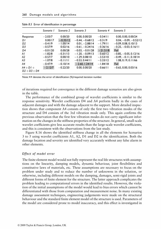
260 Damage mode ls and a lgor i thms
Table 8.5 Error of identification in percentage
Scenario 1 Scenario 2 Scenario 3 Scenario 4 Scenario 5
Response −2.03/7 0.00/20 0.00, 0.00/20 −0.54/11 0.00, 0.00, 0.00/24D1 0.00/17 −0.35/12 −0.44, −0.68/12 −0.31/9 0.04, −0.09, −0.52/12D2 −0.41/9 −1.00/14 0.01, −2.88/14 −1.79/11 −0.09, 0.08, 0.10/13D3 −0.57/9 0.02/16 −0.61, −0.24/16 −0.36/16 −0.25, −0.03, 0.16/11D4 −0.01/20 0.00/28 −0.03, −0.01/28 −21.51/8 FailA1 −1.82/8 −0.31/13 −1.20, −0.09/13 −0.60/12 −0.85, −0.05, 0.12/16A2 −0.57/7 0.00/10 −1.29, 0.08/10 −3.53/10 −0.49, −0.11, 0.18/14A3 −1.07/8 −0.11/11 −0.53, 0.44/11 −3.33/12 1.08, 0.19, 0.11/66A4 −0.47/9 −0.10/14 −2.60, 1.24/14 −1.84/18 FailA4 + D1 + −2.12/7 −0.22/20 0.00, 0.00/20 −0.66/11 −0.65, 0.00, 0.03/16D2 + D3 + D4
Note: •/• denotes the error of identification (%)/required iteration number.
of iterations required for convergence in the different damage scenarios are also givenin the table.
The performance of the combined group of wavelet coefficients is similar to theresponse sensitivity. Wavelet coefficients D4 and A4 perform badly in the cases ofadjacent damages and with the damage adjacent to the support. More detailed inspec-tion shows that component A4 consists of only the first two vibration modes of thestructure and D4 consists of the 3rd vibration mode only. This again confirms theprevious observation that the first few vibration modes do not carry significant infor-mation on the changes in the stiffness properties of the structure. In general, small-scalewavelet coefficients give less accurate results than the large-scale wavelet coefficients,and this is consistent with the observations from the last study.
Figure 8.16 shows the identified stiffness change in all the elements for Scenarios3 to 5 using wavelet coefficients A1, A2, D1 and D2 in the identification. Both thedamage location and severity are identified very accurately without any false alarm inother elements.
Ef fec t o f mode l er ror
The finite element model would not fully represent the real life structures with assump-tions on the linearity, damping models, dynamic behaviour, joint flexibilities andconstitutive laws of materials, etc. These assumptions are necessary to focus on theproblem under study and to reduce the number of unknowns in the solution, orotherwise, including different models on the damping, damages, semi-rigid joints anddifferent forms of finite element for the structure. The latter approach complicates theproblem leading to computational errors in the identified results. However, the viola-tion of the initial assumptions of the model would lead to bias errors which cannot bedifferentiated with those from computation and measurement noise. In many existingdamage assessment techniques, engineering judgements were made on the structuralbehaviour and the standard finite element model of the structure is used. Parameters ofthe model are considered prone to model inaccuracy, and this effect is investigated in
© 2009 Taylor & Francis Group, London, UK
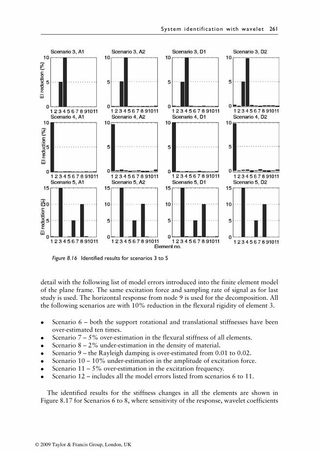
System ident i f i ca t ion wi th wave let 261
Figure 8.16 Identified results for scenarios 3 to 5
detail with the following list of model errors introduced into the finite element modelof the plane frame. The same excitation force and sampling rate of signal as for laststudy is used. The horizontal response from node 9 is used for the decomposition. Allthe following scenarios are with 10% reduction in the flexural rigidity of element 3.
• Scenario 6 – both the support rotational and translational stiffnesses have beenover-estimated ten times.
• Scenario 7 – 5% over-estimation in the flexural stiffness of all elements.• Scenario 8 – 2% under-estimation in the density of material.• Scenario 9 – the Rayleigh damping is over-estimated from 0.01 to 0.02.• Scenario 10 – 10% under-estimation in the amplitude of excitation force.• Scenario 11 – 5% over-estimation in the excitation frequency.• Scenario 12 – includes all the model errors listed from scenarios 6 to 11.
The identified results for the stiffness changes in all the elements are shown inFigure 8.17 for Scenarios 6 to 8, where sensitivity of the response, wavelet coefficients
© 2009 Taylor & Francis Group, London, UK
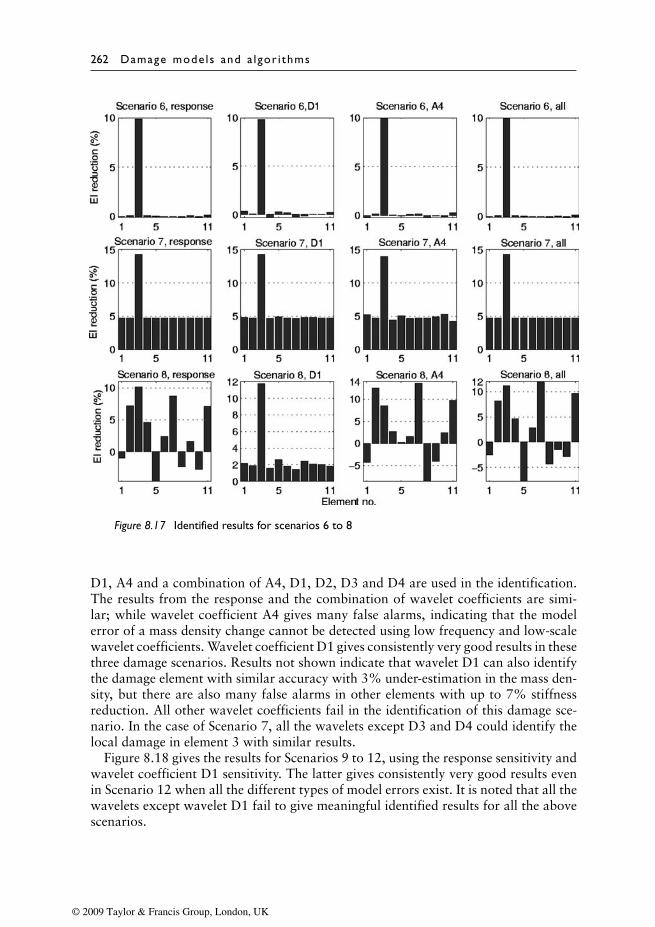
262 Damage mode ls and a lgor i thms
Figure 8.17 Identified results for scenarios 6 to 8
D1, A4 and a combination of A4, D1, D2, D3 and D4 are used in the identification.The results from the response and the combination of wavelet coefficients are simi-lar; while wavelet coefficient A4 gives many false alarms, indicating that the modelerror of a mass density change cannot be detected using low frequency and low-scalewavelet coefficients. Wavelet coefficient D1 gives consistently very good results in thesethree damage scenarios. Results not shown indicate that wavelet D1 can also identifythe damage element with similar accuracy with 3% under-estimation in the mass den-sity, but there are also many false alarms in other elements with up to 7% stiffnessreduction. All other wavelet coefficients fail in the identification of this damage sce-nario. In the case of Scenario 7, all the wavelets except D3 and D4 could identify thelocal damage in element 3 with similar results.
Figure 8.18 gives the results for Scenarios 9 to 12, using the response sensitivity andwavelet coefficient D1 sensitivity. The latter gives consistently very good results evenin Scenario 12 when all the different types of model errors exist. It is noted that all thewavelets except wavelet D1 fail to give meaningful identified results for all the abovescenarios.
© 2009 Taylor & Francis Group, London, UK
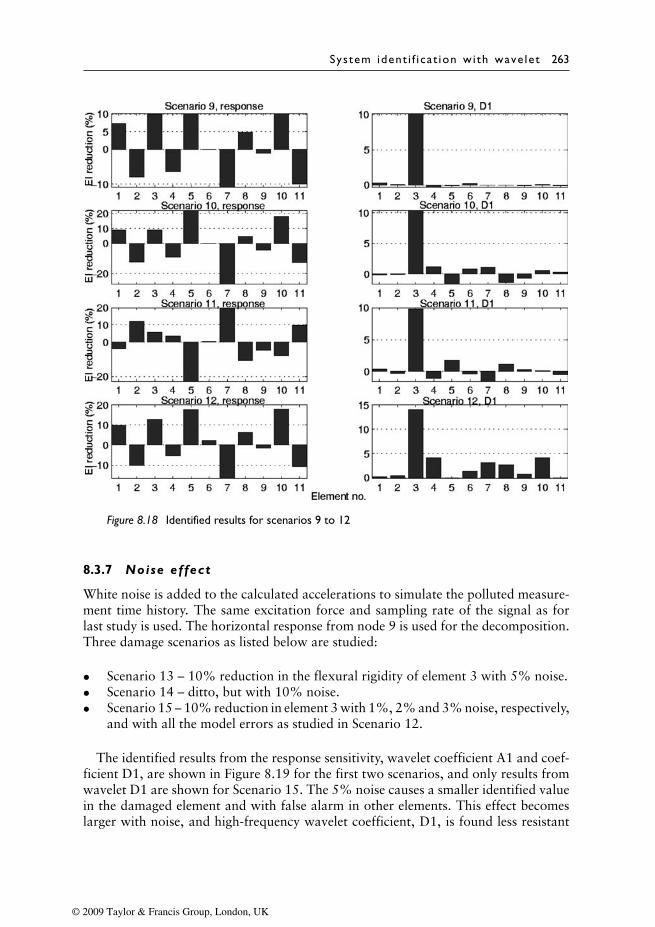
System ident i f i ca t ion wi th wave let 263
Figure 8.18 Identified results for scenarios 9 to 12
8.3.7 Noise effect
White noise is added to the calculated accelerations to simulate the polluted measure-ment time history. The same excitation force and sampling rate of the signal as forlast study is used. The horizontal response from node 9 is used for the decomposition.Three damage scenarios as listed below are studied:
• Scenario 13 – 10% reduction in the flexural rigidity of element 3 with 5% noise.• Scenario 14 – ditto, but with 10% noise.• Scenario 15 – 10% reduction in element 3 with 1%, 2% and 3% noise, respectively,
and with all the model errors as studied in Scenario 12.
The identified results from the response sensitivity, wavelet coefficient A1 and coef-ficient D1, are shown in Figure 8.19 for the first two scenarios, and only results fromwavelet D1 are shown for Scenario 15. The 5% noise causes a smaller identified valuein the damaged element and with false alarm in other elements. This effect becomeslarger with noise, and high-frequency wavelet coefficient, D1, is found less resistant
© 2009 Taylor & Francis Group, London, UK
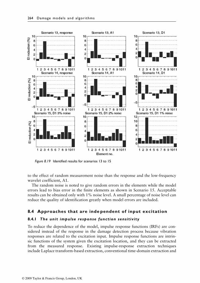
264 Damage mode ls and a lgor i thms
Figure 8.19 Identified results for scenarios 13 to 15
to the effect of random measurement noise than the response and the low-frequencywavelet coefficient, A1.
The random noise is noted to give random errors in the elements while the modelerrors lead to bias error in the finite elements as shown in Scenario 15. Acceptableresults can be obtained only with 1% noise level. A small percentage of noise level canreduce the quality of identification greatly when model errors are included.
8.4 Approaches that are inde pendent of input excitation
8.4.1 The unit impulse response function sensit iv ity
To reduce the dependence of the model, impulse response functions (IRFs) are con-sidered instead of the response in the damage detection process because vibrationresponses are related to the excitation input. Impulse response functions are intrin-sic functions of the system given the excitation location, and they can be extractedfrom the measured response. Existing impulse-response extraction techniquesinclude Laplace transform-based extraction, conventional time-domain extraction and
© 2009 Taylor & Francis Group, London, UK
System ident i f i ca t ion wi th wave let 265
FFT-based extraction (Robertson et al., 1998). FFT-based extraction is most commonlyused to obtain the impulse response function. However, it has long been recognizedthat FFT-based vibration signal analysis exhibits several weakness.
In contrast to the FFT-based extraction procedure, which must process the datain both the time and frequency domains, the discrete wavelet transform (DWT)-basedextraction procedure (Robertson et al., 1998) handles the experimental data only in thetime domain. This involves the forward and inverse DWT plus an inversion operation,and is indeed preferable.
8.4.1.1 Wavelet-based un i t impulse response
The equation of motion of a N DOFs damped structural system under the unit impulseexcitation is
M••x + C
•x + Kx = Dδ(t) (8.61)
where M, C and K are the N × N mass, damping and stiffness matrices, respectively;N is the number of DOFs of the system; D is the mapping matrix relating the forceexcitation location to the corresponding DOFs of the system; x,
•x and
••x are the N × 1
displacement, velocity and acceleration vectors, respectively; and δ(t) is the Diracdelta function. Assuming the system is in static equilibrium before the unit impulseexcitation, then the forced vibration system with the unit impulse excitation can beconverted to a free vibration system with the following initial conditions,
x(0) = 0,•x(0) = M−1D (8.62)
Rewriting Equations (8.61) and (8.62), the unit impulse response function can becomputed from the following:M
••h + C
•h + Kh = 0
h(0) = 0,•h(0) = M−1D
(8.63)
where h,•h and
••h are the unit impulse displacement, velocity and acceleration vectors,
respectively. Using the Newmark method, the unit impulse response can easily becomputed.
Expressing the local damage in the structural system in the form of �K =∑nei=1αiKi,
where αi is the fractional change in the stiffness of an element, and ne is the numberof elements in the structure. Differentiating Equation (8.63) with respect to αi, gives
M∂
••h∂αi
+ C∂
•h∂αi
+ K∂h∂αi
= − ∂K∂αi
h
∂h(0)∂αi
= 0,∂
•h(0)∂αi
= ∂M−1D∂αi
(8.64)
© 2009 Taylor & Francis Group, London, UK
266 Damage mode ls and a lgor i thms
The sensitivities ∂h/∂αi, ∂•h/∂αi and ∂
••h/∂αi can then be obtained from Equation (8.64)
with Newmark Method.A signal can be expressed by the Discrete Wavelet Transform (DWT) in terms of
the local basis functions (Daubechies, 1992). Daubechies wavelets are used in thefollowing studies as they satisfy the two crucial requirements: the orthogonality oflocal basis functions and second-order accuracy or higher, depending on the dilationexpression adopted.
A function f (t) can therefore be approximated in terms of its DWT as
f (t) = f DWT0 ϕ(t) + f DWT
1 ψ(t) + f DWT2 ψ(2t) + · · · + f DWT
2j+k ψ(2jt − k) (8.65)
where ϕ(t) and ψ(t)are the scaling function and the mother wavelet function,respectively, and they satisfy the following relations,
ϕ(t) = √2
+∞∑k=−∞
h(k)ϕ(2t − k); ψ(t) = √2
+∞∑k=−∞
g(k)ϕ(2t − k);
ψj,k(t) = 2− j2ψ(2−jt − k) (8.66)
where h(k) and g(k) are the low-pass and high-pass analysis filters, respectively, whichare all constants; and f DWT
2j+kis the wavelet transform coefficients. Because of the orthog-
onality on both the translation and scale of the Daubechies wavelets, the following isobtained,∫
ψj,k(t)ψm,n(t)dt =δj,mδk,n (8.67)
Thus, for real wavelets from Equations (8.65) and (8.67),
f DWT0 =
∫f (t)ϕ(t)dt; f DWT
2j+k =∫
f (t)ψj,k(t)dt (8.68)
The wavelet coefficient of the impulse-response function sensitivity has been shown(Law et al., 2006) equal to the first derivative of the wavelet coefficients of the impulse-response function with respect to the damage parameter, αi, i.e.
DWT
∂••h∂αi
= ∂••h
DWT
∂αi(8.69)
where DWT(∂••h/∂αi) is the discrete wavelet coefficient of ∂
••h/∂αi. Therefore differen-
tiating the second part of Equation (8.68) with respect to the stiffness parameter of anelement gives ∂••
h∂αi
DWT
2j+k
=∫∂
••h∂αiψj,k(t)dt (8.70)
© 2009 Taylor & Francis Group, London, UK
System ident i f i ca t ion wi th wave let 267
The sensitivity matrix can then be formed from Equation (8.70) as
S =[∂
••h
DWT
l
∂α1
∂••h
DWT
l
∂α2· · · ∂
••h
DWT
l
∂αm
](8.71)
where••h
DWT
l is the DWT coefficient of••hl;
••hl denotes the acceleration impulse response
function at location l; and m is the number of structural parameters.
8.4.1.2 Impulse response funct ion v ia d i screte wave le t t rans form
The equation of motion of an N DOFs damped structural system under generalexcitation is written as
M••x + C
•x + Kx = DF(t) (8.72)
where F(t) is the vector of excitation force. If the system has zero initial conditions,the solution of Equation (8.72) can be expressed as,
x(t) =∫ t
0h(t − τ)F(τ)dτ (8.73)
The acceleration response,••xl(tn), from location l at time tn is,
••xl(tn) =
∫ tn
0
••hl(τ) · F(tn − τ)dτ (8.74)
Applying DWT to••hl(τ) and F(tn − τ) respectively, gives
••hl(τ) = ••
hDWT
l,0 ϕ(τ) + ••h
DWT
l,1 ψ(τ) + · · · + ••h
DWT
l,2j+kψ(2jτ − k) (8.75)
F(tn − τ) = FDWT0 (tn)ϕ(τ) + FDWT
1 (tn)ψ(τ) + · · · + FDWT2j+k (tn)ψ(2jτ − k) (8.76)
Substituting Equations (8.75) and (8.76) into Equation (8.74),
••xl(tn) =
∫ tn
0(••h
DWT
l,0 ϕ(τ) + ••h
DWT
l,1 ψ(τ) + · · · + ••h
DWT
l,2j+kψ(2jτ − k))
× (FDWT0 (tn)ϕ(τ) + FDWT
1 (tn)ψ(τ) + · · · + FDWT2j+k (tn)ψ(2jτ − k))dτ
(8.77)
© 2009 Taylor & Francis Group, London, UK
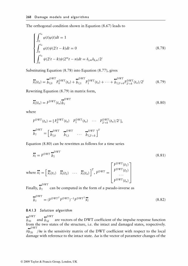
268 Damage mode ls and a lgor i thms
The orthogonal condition shown in Equation (8.67) leads to
∫ tn
0ϕ(t)ϕ(t)dt = 1∫ tn
0ϕ(t)ψ(2jt − k)dt = 0∫ tn
0ψ(2jt − k)ψ(2mt − n)dt = δj,mδk,n/2j
(8.78)
Substituting Equation (8.78) into Equation (8.77), gives
••xl(tn) = ••
hDWT
l,0 FDWT0 (tn) + ••
hDWT
l,1 FDWT1 (tn) + · · · + ••
hDWT
l,2j+kFDWT2j+k (tn)/2j (8.79)
Rewriting Equation (8.79) in matrix form,
••xl(tn) = FDWT (tn)
••h
DWT
l (8.80)
where
FDWT (tn) = [ FDWT0 (tn) FDWT
1 (tn) · · · FDWT2j+k
(tn)/2j ],
••h
DWT
l =[ ••
hDWT
l,0
••h
DWT
l,1 · · · ••h
DWT
l,2j+k
]T
Equation (8.80) can be rewritten as follows for a time series
••xl = FDWT
••h
DWT
l (8.81)
where••xl =
[ ••xl(t1)
••xl(t2) · · · ••
xl(tn)]T
, FDWT =
FDWT (t1)
FDWT (t2)· · ·
FDWT (tn)
Finally,
••h
DWT
l can be computed in the form of a pseudo-inverse as
••h
DWT
l = (FDWTTFDWT )−1FDWTT ••
xl (8.82)
8.4.1.3 So lut ion a lgor i thm
••h
DWT
l0 and••h
DWT
ld are vectors of the DWT coefficient of the impulse response functionfrom the two states of the structure, i.e. the intact and damaged states, respectively.
∂••h
DWT
l0 /∂α is the sensitivity matrix of the DWT coefficient with respect to the localdamage with reference to the intact state. �α is the vector of parameter changes of the
© 2009 Taylor & Francis Group, London, UK
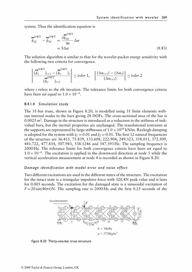
System ident i f i ca t ion wi th wave let 269
system. Thus the identification equation is
••h
DWT
ld − ••h
DWT
l0 = ∂••h
DWT
l0
∂α�α
= S�α (8.83)
The solution algorithm is similar to that for the wavelet-packet energy sensitivity withthe following two criteria for convergence.∥∥∥∥∥∥ {••
hDWT
l }i+1 − {••h
DWT
l }i
{••h
DWT
l }i+1
∥∥∥∥∥∥ ≤ toler 1,∥∥∥∥ {�αi+1} − {�αi}
{�αi+1}∥∥∥∥ ≤ toler 2
where i refers to the ith iteration. The tolerance limits for both convergence criteriahave been set equal to 1.0 × 10⁻⁶.
8.4.1.4 S imulat ion s tudy
The 31-bar truss, shown in Figure 8.20, is modelled using 31 finite elements with-out internal nodes in the bars giving 28 DOFs. The cross-sectional area of the bar is0.0025 m2. Damage in the structure is introduced as a reduction in the stiffness of indi-vidual bars, but the inertial properties are unchanged. The translational restraints atthe supports are represented by large stiffnesses of 1.0 × 10¹⁰ kN/m. Rayleigh dampingis adopted for the system with ξ1 = 0.01 and ξ2 = 0.01. The first 12 natural frequenciesof the structure are 36.415, 75.839, 133.608, 222.904, 249.323, 358.011, 372.509,441.722, 477.834, 507.943, 538.1246 and 547.393 Hz. The sampling frequency is2000 Hz. The tolerance limits for both convergence criteria have been set equal to1.0 × 10−6. The excitation is applied in the downward direction at node 5 while thevertical acceleration measurement at node 4 is recorded as shown in Figure 8.20.
Damage ident i f i cat ion wi th mode l er ror and no ise ef fec t
Two different excitations are used in the different states of the structure. The excitationfor the intact state is a triangular impulsive force with 320.4N peak value and it lastsfor 0.005 seconds. The excitation for the damaged state is a sinusoidal excitation ofF = 20 sin(40πt)N. The sampling rate is 2000 Hz and the first 0.25 seconds of the
E � 70GPa3r � 2770kg/m
1
2
3
4
6
5
8
7 9
10 12
11 13
14
1.52m
1.52
m
2
1 3
4 5
6
7 8
9 10
11
1213
1415
16
1718
1920
21
2223
24 25
2926
2728
30
31
FAccelerometer
Figure 8.20 Thirty-one-bar truss structure
© 2009 Taylor & Francis Group, London, UK
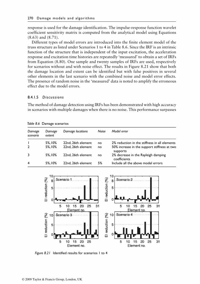
270 Damage mode ls and a lgor i thms
response is used for the damage identification. The impulse-response function waveletcoefficient sensitivity matrix is computed from the analytical model using Equations(8.63) and (8.71).
Different types of model errors are introduced into the finite element model of thetruss structure as listed under Scenarios 1 to 4 in Table 8.6. Since the IRF is an intrinsicfunction of the structure that is independent of the input excitation, the accelerationresponse and excitation time histories are repeatedly ‘measured’ to obtain a set of IRFsfrom Equation (8.80). One sample and twenty samples of IRFs are used, respectivelyfor scenarios without and with noise effect. The results in Figure 8.21 show that boththe damage location and extent can be identified but with false positives in severalother elements in the last scenario with the combined noise and model error effects.The presence of random noise in the ‘measured’ data is noted to amplify the erroneouseffect due to the model errors.
8.4.1.5 Discuss ions
The method of damage detection using IRFs has been demonstrated with high accuracyin scenarios with multiple damages when there is no noise. This performance surpasses
Table 8.6 Damage scenarios
Damage Damage Damage locations Noise Model errorscenario extent
1 5%,10% 22nd, 26th element no 2% reduction in the stiffness in all elements2 5%,10% 22nd, 26th element no 50% increase in the support stiffness at two
supports3 5%,10% 22nd, 26th element no 2% decrease in the Rayleigh damping
coefficients4 5%,10% 22nd, 26th element 5% Include all the above model errors
Figure 8.21 Identified results for scenarios 1 to 4
© 2009 Taylor & Francis Group, London, UK
System ident i f i ca t ion wi th wave let 271
those from other existing damage detection methods. But the identified results sufferfrom the accompanying noise effect and initial model errors when dealing with realstructures. The noise effect can be further reduced by averaging and taking a longerduration of measurement from more and better-located sensors. However, the initialmodel errors associated with a fixture in a joint, material nonlinearity, cracks andfissures in a member, etc. cannot be addressed with the present approach of modellingthe damage with an averaged damage parameter. Separate damage models shouldbe included in the initial model for proper identification. However, the wavelet isknown to have a broad bandwidth of responses, and further benefit can be sought byemploying sensitivity for wavelets from different bandwidths in the inverse analysis,as the noise effect and model error would have different contributions to the differentbandwidth of the responses (Law et al., 2006).
8.4.2 The covariance sensit iv ity
This section presents one approach which is different to that shown in Section 8.4.1 fora general type of excitation. The excitation under consideration is ambient white noiseexcitation, which usually exists in the environment with large-scale infrastructures. Thecovariance of responses is expressed explicitly as a function of the impulse responsefunction of the system under single or multiple ambient excitations. The sensitivity ofthe covariance of responses with respect to the physical parameters of the structure isderived analytically.
8.4.2.1 Covar iance of measured responses
The equation of motion of the NDOFs damped structural system under generalexcitation is
M••x + C
•x + Kx = DkFk(t) (8.84)
where Fk(t) is the excitation force at the kth DOF. If the system has zero initialconditions, the solution of Equation (8.84) can be expressed as,
xk(t) =∫ t
−∞hk(t − τ)Fk(τ)dτ (8.85)
where hk(t) is the vector of impulse response of the system under a unit impulse exci-tation at the kth DOF. The measured acceleration responses
••xpk(t) from location p at
time t and••xqk(t + τ) from location q at time t + τ are, respectively,
••xpk(t) =
∫ t
−∞
••hpk(t − σ)Fk(σ)dσ,
••xqk(t + τ) =
∫ t+τ
−∞
••hqk(t + τ − σ)Fk(σ)dσ
(8.86)
The cross-correlation function, Rpqk(τ), relating the two measured responses is givenby Bendat and Piersol (1980) as
Rpqk(τ) = E{••xpk(t)
••xqk(t + τ)} (8.87)
© 2009 Taylor & Francis Group, London, UK
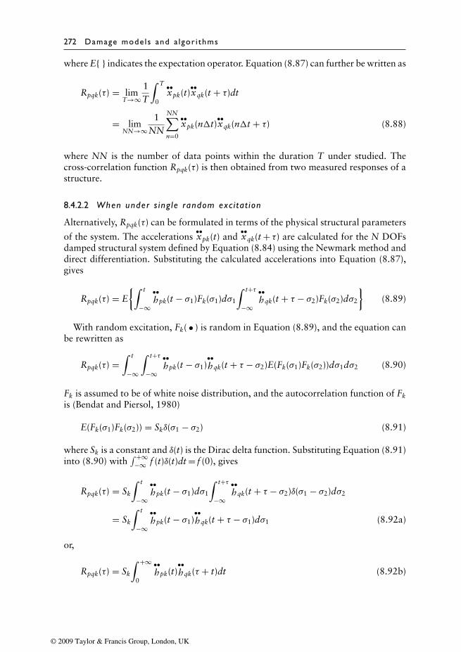
272 Damage mode ls and a lgor i thms
where E{ } indicates the expectation operator. Equation (8.87) can further be written as
Rpqk(τ) = limT→∞
1T
∫ T
0
••xpk(t)
••xqk(t + τ)dt
= limNN→∞
1NN
NN∑n=0
••xpk(n�t)
••xqk(n�t + τ) (8.88)
where NN is the number of data points within the duration T under studied. Thecross-correlation function Rpqk(τ) is then obtained from two measured responses of astructure.
8.4.2.2 When under s ing le random exc i ta t ion
Alternatively, Rpqk(τ) can be formulated in terms of the physical structural parameters
of the system. The accelerations••xpk(t) and
••xqk(t + τ) are calculated for the N DOFs
damped structural system defined by Equation (8.84) using the Newmark method anddirect differentiation. Substituting the calculated accelerations into Equation (8.87),gives
Rpqk(τ) = E{∫ t
−∞
••hpk(t − σ1)Fk(σ1)dσ1
∫ t+τ
−∞
••hqk(t + τ − σ2)Fk(σ2)dσ2
}(8.89)
With random excitation, Fk( • ) is random in Equation (8.89), and the equation canbe rewritten as
Rpqk(τ) =∫ t
−∞
∫ t+τ
−∞
••hpk(t − σ1)
••hqk(t + τ − σ2)E(Fk(σ1)Fk(σ2))dσ1dσ2 (8.90)
Fk is assumed to be of white noise distribution, and the autocorrelation function of Fk
is (Bendat and Piersol, 1980)
E(Fk(σ1)Fk(σ2)) = Skδ(σ1 − σ2) (8.91)
where Sk is a constant and δ(t) is the Dirac delta function. Substituting Equation (8.91)into (8.90) with
∫ +∞−∞ f (t)δ(t)dt = f (0), gives
Rpqk(τ) = Sk
∫ t
−∞
••hpk(t − σ1)dσ1
∫ t+τ
−∞
••hqk(t + τ − σ2)δ(σ1 − σ2)dσ2
= Sk
∫ t
−∞
••hpk(t − σ1)
••hqk(t + τ − σ1)dσ1 (8.92a)
or,
Rpqk(τ) = Sk
∫ +∞
0
••hpk(t)
••hqk(τ + t)dt (8.92b)
© 2009 Taylor & Francis Group, London, UK
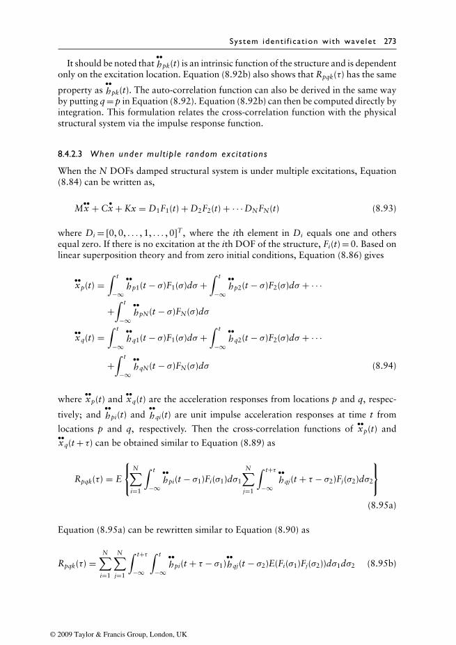
System ident i f i ca t ion wi th wave let 273
It should be noted that••hpk(t) is an intrinsic function of the structure and is dependent
only on the excitation location. Equation (8.92b) also shows that Rpqk(τ) has the same
property as••hpk(t). The auto-correlation function can also be derived in the same way
by putting q = p in Equation (8.92). Equation (8.92b) can then be computed directly byintegration. This formulation relates the cross-correlation function with the physicalstructural system via the impulse response function.
8.4.2.3 When under mul t ip le random exc i ta t ions
When the N DOFs damped structural system is under multiple excitations, Equation(8.84) can be written as,
M••x + C
•x + Kx = D1F1(t) + D2F2(t) + · · · DNFN(t) (8.93)
where Di = [0, 0, . . . , 1, . . . , 0]T , where the ith element in Di equals one and othersequal zero. If there is no excitation at the ith DOF of the structure, Fi(t) = 0. Based onlinear superposition theory and from zero initial conditions, Equation (8.86) gives
••xp(t) =
∫ t
−∞
••hp1(t − σ)F1(σ)dσ +
∫ t
−∞
••hp2(t − σ)F2(σ)dσ + · · ·
+∫ t
−∞
••hpN(t − σ)FN(σ)dσ
••xq(t) =
∫ t
−∞
••hq1(t − σ)F1(σ)dσ +
∫ t
−∞
••hq2(t − σ)F2(σ)dσ + · · ·
+∫ t
−∞
••hqN(t − σ)FN(σ)dσ (8.94)
where••xp(t) and
••xq(t) are the acceleration responses from locations p and q, respec-
tively; and••hpi(t) and
••hqi(t) are unit impulse acceleration responses at time t from
locations p and q, respectively. Then the cross-correlation functions of••xp(t) and
••xq(t + τ) can be obtained similar to Equation (8.89) as
Rpqk(τ) = E
N∑
i=1
∫ t
−∞
••hpi(t − σ1)Fi(σ1)dσ1
N∑j=1
∫ t+τ
−∞
••hqj(t + τ − σ2)Fj(σ2)dσ2
(8.95a)
Equation (8.95a) can be rewritten similar to Equation (8.90) as
Rpqk(τ) =N∑
i=1
N∑j=1
∫ t+τ
−∞
∫ t
−∞
••hpi(t + τ − σ1)
••hqj(t − σ2)E(Fi(σ1)Fj(σ2))dσ1dσ2 (8.95b)
© 2009 Taylor & Francis Group, London, UK
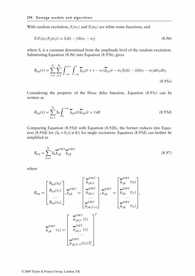
274 Damage mode ls and a lgor i thms
With random excitation, Fi(σ1) and Fj(σ2) are white noise functions, and
E(Fi(σ1)Fj(σ2)) = Siδ(i − j)δ(σ1 − σ2) (8.96)
where Si is a constant determined from the amplitude level of the random excitation.Substituting Equation (8.96) into Equation (8.95b), gives
Rpq(τ) =N∑
i=1
N∑j=1
∫ t+τ
−∞
∫ t
−∞
••hpi(t + τ − σ1)
••hqj(t − σ2)Siδ(i − j)δ(σ1 − σ2)dσ1dσ2
(8.95c)
Considering the property of the Dirac delta function, Equation (8.95c) can bewritten as
Rpq(τ) =N∑
k=1
Sk
∫ +∞
0
••hpk(t)
••hqk(t + τ)dt (8.95d)
Comparing Equation (8.95d) with Equation (8.92b), the former reduces into Equa-tion (8.95d) for (Sk = 0, (i = k)) for single excitation. Equation (8.95d) can further besimplified as
Rpq =N∑
k=1
Sk
••h
DWT
qk
••h
DWT
pk (8.97)
where
Rpq =
Rpq(τ0)
Rpq(τ1)
· · ·Rpq(τn)
,••h
DWT
pk =
••h
DWT
pk,0
••h
DWT
pk,1
· · ·••h
DWT
pk,2j+l
,••h
DWT
qk =
••h
DWT
qk (τ0)
••h
DWT
qk (τ1)· · ·
••h
DWT
qk (τn)
,
••h
DWT
qk (τi) =
••h
DWT
qk,0 (τi)
••h
DWT
qk,1 (τi)· · ·
••h
DWT
qk,2j+l(τi)/2j
T
© 2009 Taylor & Francis Group, London, UK
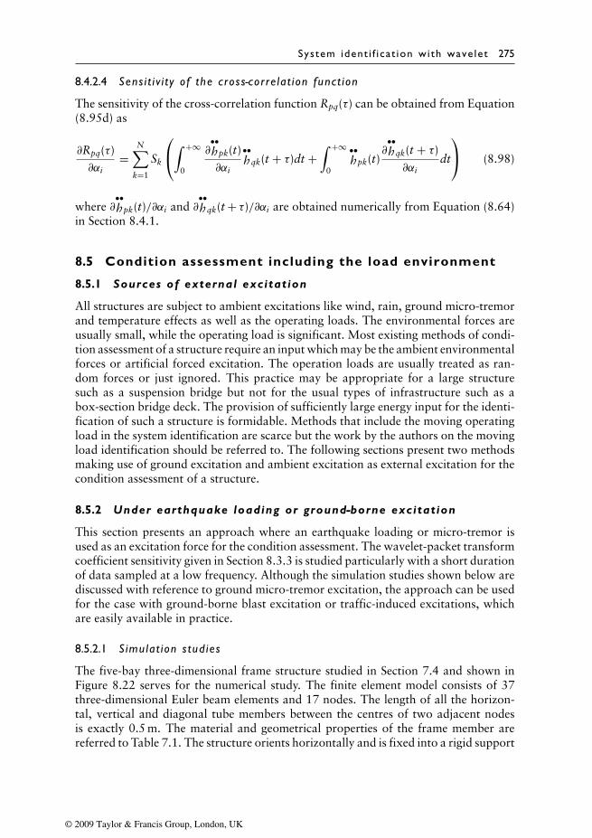
System ident i f i ca t ion wi th wave let 275
8.4.2.4 Sens i t i v i t y o f the cross-corre la t ion funct ion
The sensitivity of the cross-correlation function Rpq(τ) can be obtained from Equation(8.95d) as
∂Rpq(τ)∂αi
=N∑
k=1
Sk
∫ +∞
0
∂••hpk(t)∂αi
••hqk(t + τ)dt +
∫ +∞
0
••hpk(t)
∂••hqk(t + τ)∂αi
dt
(8.98)
where ∂••hpk(t)/∂αi and ∂
••hqk(t + τ)/∂αi are obtained numerically from Equation (8.64)
in Section 8.4.1.
8.5 Condition assessment including the load environment
8.5.1 Sources of external excitation
All structures are subject to ambient excitations like wind, rain, ground micro-tremorand temperature effects as well as the operating loads. The environmental forces areusually small, while the operating load is significant. Most existing methods of condi-tion assessment of a structure require an input which may be the ambient environmentalforces or artificial forced excitation. The operation loads are usually treated as ran-dom forces or just ignored. This practice may be appropriate for a large structuresuch as a suspension bridge but not for the usual types of infrastructure such as abox-section bridge deck. The provision of sufficiently large energy input for the identi-fication of such a structure is formidable. Methods that include the moving operatingload in the system identification are scarce but the work by the authors on the movingload identification should be referred to. The following sections present two methodsmaking use of ground excitation and ambient excitation as external excitation for thecondition assessment of a structure.
8.5.2 Under earthquake loading or ground-borne excitation
This section presents an approach where an earthquake loading or micro-tremor isused as an excitation force for the condition assessment. The wavelet-packet transformcoefficient sensitivity given in Section 8.3.3 is studied particularly with a short durationof data sampled at a low frequency. Although the simulation studies shown below arediscussed with reference to ground micro-tremor excitation, the approach can be usedfor the case with ground-borne blast excitation or traffic-induced excitations, whichare easily available in practice.
8.5.2.1 S imulat ion s tud ies
The five-bay three-dimensional frame structure studied in Section 7.4 and shown inFigure 8.22 serves for the numerical study. The finite element model consists of 37three-dimensional Euler beam elements and 17 nodes. The length of all the horizon-tal, vertical and diagonal tube members between the centres of two adjacent nodesis exactly 0.5 m. The material and geometrical properties of the frame member arereferred to Table 7.1. The structure orients horizontally and is fixed into a rigid support
© 2009 Taylor & Francis Group, London, UK
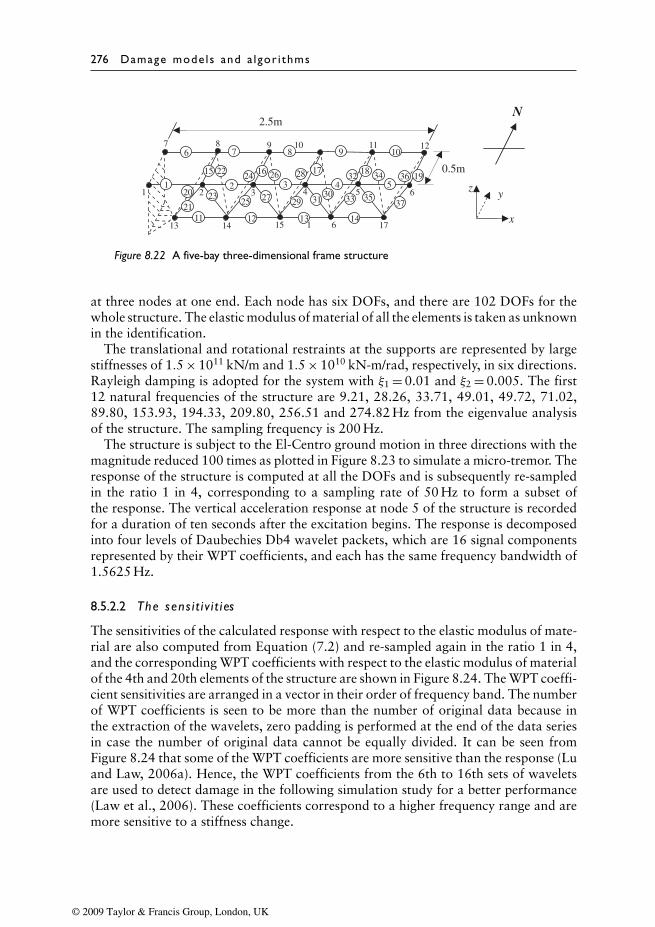
276 Damage mode ls and a lgor i thms
x
z y1 2 3 4 5 6
7 8 9 10 11 12
13 14 15 1 6 17
1 2 3 4 5
7 8 9 106
11 12 13 14
15 16 17 1819
20
21
22
23
24 26
25 27
28
2930
31
32
33
34
35
36
37
2.5m
0.5m
N
Figure 8.22 A five-bay three-dimensional frame structure
at three nodes at one end. Each node has six DOFs, and there are 102 DOFs for thewhole structure. The elastic modulus of material of all the elements is taken as unknownin the identification.
The translational and rotational restraints at the supports are represented by largestiffnesses of 1.5 × 10¹¹ kN/m and 1.5 × 10¹⁰ kN-m/rad, respectively, in six directions.Rayleigh damping is adopted for the system with ξ1 = 0.01 and ξ2 = 0.005. The first12 natural frequencies of the structure are 9.21, 28.26, 33.71, 49.01, 49.72, 71.02,89.80, 153.93, 194.33, 209.80, 256.51 and 274.82 Hz from the eigenvalue analysisof the structure. The sampling frequency is 200 Hz.
The structure is subject to the El-Centro ground motion in three directions with themagnitude reduced 100 times as plotted in Figure 8.23 to simulate a micro-tremor. Theresponse of the structure is computed at all the DOFs and is subsequently re-sampledin the ratio 1 in 4, corresponding to a sampling rate of 50 Hz to form a subset ofthe response. The vertical acceleration response at node 5 of the structure is recordedfor a duration of ten seconds after the excitation begins. The response is decomposedinto four levels of Daubechies Db4 wavelet packets, which are 16 signal componentsrepresented by their WPT coefficients, and each has the same frequency bandwidth of1.5625 Hz.
8.5.2.2 The sens i t i v i t i es
The sensitivities of the calculated response with respect to the elastic modulus of mate-rial are also computed from Equation (7.2) and re-sampled again in the ratio 1 in 4,and the corresponding WPT coefficients with respect to the elastic modulus of materialof the 4th and 20th elements of the structure are shown in Figure 8.24. The WPT coeffi-cient sensitivities are arranged in a vector in their order of frequency band. The numberof WPT coefficients is seen to be more than the number of original data because inthe extraction of the wavelets, zero padding is performed at the end of the data seriesin case the number of original data cannot be equally divided. It can be seen fromFigure 8.24 that some of the WPT coefficients are more sensitive than the response (Luand Law, 2006a). Hence, the WPT coefficients from the 6th to 16th sets of waveletsare used to detect damage in the following simulation study for a better performance(Law et al., 2006). These coefficients correspond to a higher frequency range and aremore sensitive to a stiffness change.
© 2009 Taylor & Francis Group, London, UK
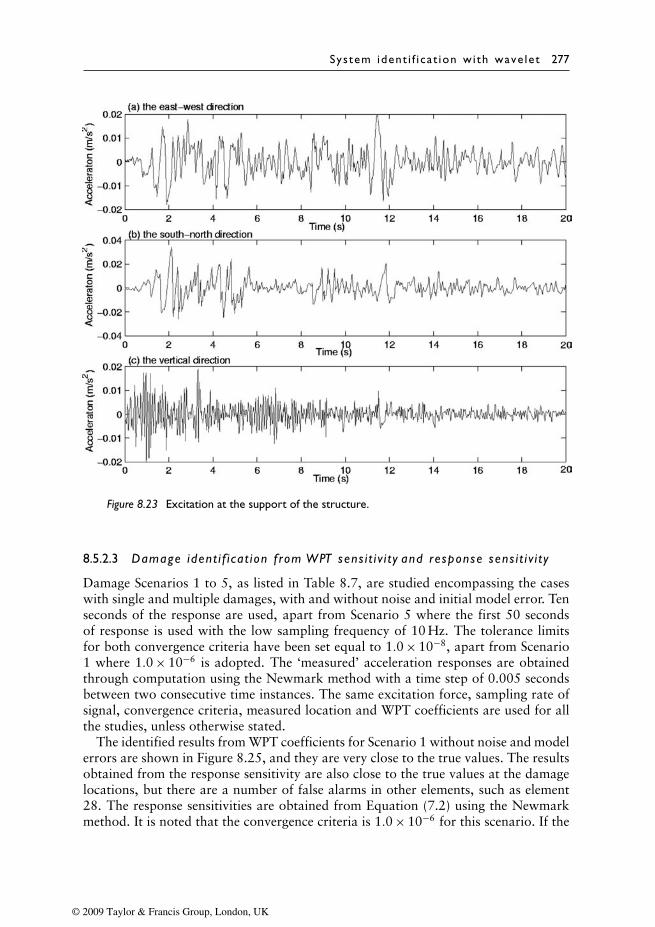
System ident i f i ca t ion wi th wave let 277
Figure 8.23 Excitation at the support of the structure.
8.5.2.3 Damage ident i f i cat ion f rom WPT sens i t i v i t y and response sens i t i v i t y
Damage Scenarios 1 to 5, as listed in Table 8.7, are studied encompassing the caseswith single and multiple damages, with and without noise and initial model error. Tenseconds of the response are used, apart from Scenario 5 where the first 50 secondsof response is used with the low sampling frequency of 10 Hz. The tolerance limitsfor both convergence criteria have been set equal to 1.0 × 10⁻⁸, apart from Scenario1 where 1.0 × 10⁻⁶ is adopted. The ‘measured’ acceleration responses are obtainedthrough computation using the Newmark method with a time step of 0.005 secondsbetween two consecutive time instances. The same excitation force, sampling rate ofsignal, convergence criteria, measured location and WPT coefficients are used for allthe studies, unless otherwise stated.
The identified results from WPT coefficients for Scenario 1 without noise and modelerrors are shown in Figure 8.25, and they are very close to the true values. The resultsobtained from the response sensitivity are also close to the true values at the damagelocations, but there are a number of false alarms in other elements, such as element28. The response sensitivities are obtained from Equation (7.2) using the Newmarkmethod. It is noted that the convergence criteria is 1.0 × 10⁻⁶ for this scenario. If the
© 2009 Taylor & Francis Group, London, UK
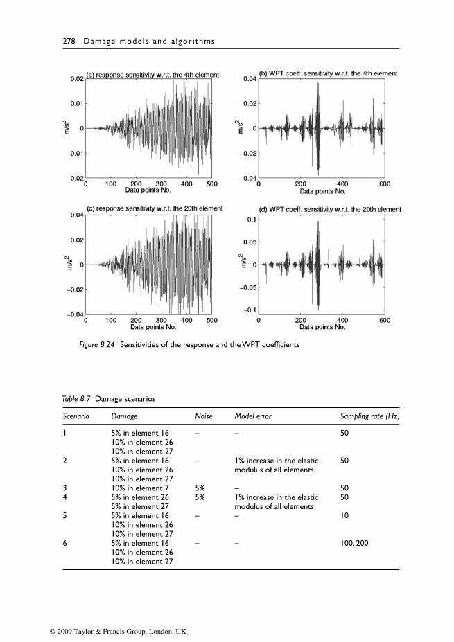
278 Damage mode ls and a lgor i thms
Figure 8.24 Sensitivities of the response and the WPT coefficients
Table 8.7 Damage scenarios
Scenario Damage Noise Model error Sampling rate (Hz)
1 5% in element 16 – – 5010% in element 2610% in element 27
2 5% in element 16 – 1% increase in the elastic 5010% in element 26 modulus of all elements10% in element 27
3 10% in element 7 5% – 504 5% in element 26 5% 1% increase in the elastic 50
5% in element 27 modulus of all elements5 5% in element 16 – – 10
10% in element 2610% in element 27
6 5% in element 16 – – 100, 20010% in element 2610% in element 27
© 2009 Taylor & Francis Group, London, UK
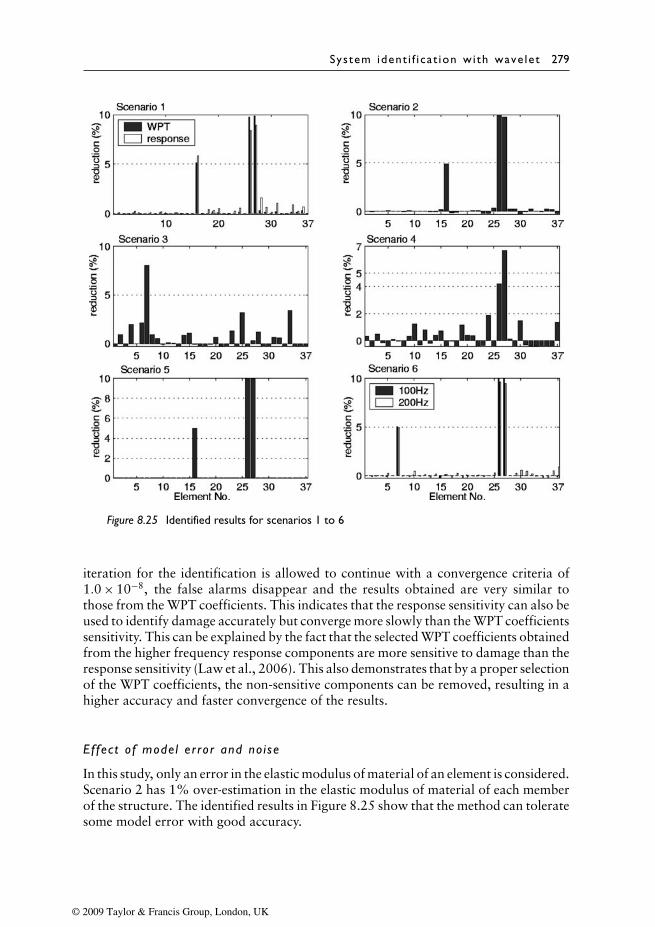
System ident i f i ca t ion wi th wave let 279
Figure 8.25 Identified results for scenarios 1 to 6
iteration for the identification is allowed to continue with a convergence criteria of1.0 × 10−8, the false alarms disappear and the results obtained are very similar tothose from the WPT coefficients. This indicates that the response sensitivity can also beused to identify damage accurately but converge more slowly than the WPT coefficientssensitivity. This can be explained by the fact that the selected WPT coefficients obtainedfrom the higher frequency response components are more sensitive to damage than theresponse sensitivity (Law et al., 2006). This also demonstrates that by a proper selectionof the WPT coefficients, the non-sensitive components can be removed, resulting in ahigher accuracy and faster convergence of the results.
Ef fec t o f mode l er ror and no ise
In this study, only an error in the elastic modulus of material of an element is considered.Scenario 2 has 1% over-estimation in the elastic modulus of material of each memberof the structure. The identified results in Figure 8.25 show that the method can toleratesome model error with good accuracy.
© 2009 Taylor & Francis Group, London, UK
280 Damage mode ls and a lgor i thms
Damage Scenario 3 has 5% noise in the ‘measured’ acceleration. The location andextent of the damage can be identified with some accuracy as shown in Figure 8.25,but there are also alarms in several adjacent elements. The random noise is noted togive error in the identified damage of the damaged element, although a good indicationof the damage location is still achieved. This shows that the identified results are easilycorrupted by measurement noise, and noise reduction prior to identification is needed.
Scenario 4 is studied with damage in two adjacent elements to test the resolu-tion capability of the approach with close proximity of two damages. The resultsin Figure 8.25 indicate that WPT coefficients can identify the damage elements quiteaccurately but with some error in the damage magnitude. It is believed that morespatial information of the structure can be captured from using responses from morelocations of the structure to mitigate the noise effect.
Per formance from a subset of the measured response
In practice, most of the on-line health monitoring systems operate with a high samplingfrequency, sufficient to cover a wide range of the structural response. Scenario 5 is onthe use of a subset of the original response re-sampled in the ratio 1 in 20. All sixteen setsof WPT coefficients are used in the identification. The identified results in Figure 8.25show that this subset of the ‘measured’ response yields very accurate results.
It should be noted that for all the Scenarios in Table 8.7, the response obtained fromthe equation of motion of the structure contains components from all the structuralvibration modes with frequencies below 100 Hz, and the re-sampling of the responseonly results in a subset of the response measurement. The time-domain approach doesnot depend mainly on the frequency information of the measured response as thefrequency-domain method does, and it also makes use of the vibration amplitude inthe solution process as in the following discussions.
The amplitude of the structural response, when expressed in the form of a Duhamelintegral of
∑ni=1
∫ e−ξiωiτ
ωidsin (ωidτ) · F(t − τ)dτ, includes the structural information
in the two terms of sin (ωidτ) and e−ξiωiτ/ωid. The Nyquist frequency has to be sat-isfied if the structural vibration information (both the amplitude and frequency) issought from the term sin (ωidτ). However, the term e−ξnωnτ is an exponential functionand is independent of the sampling frequency. The time-domain method is thereforeless dependent on the Nyquist frequency and the damage detection can be performedsuccessfully with a low sampling rate.
Another comparison is made in Scenario 6 with two sets of responses. The first setis computed from Equation (7.1) with a sampling rate of 200 Hz, and the other set isobtained from re-sampling the first set of response in the ratio 1 in 2. The first eight setsof WPT coefficients from the first set and all sixteen sets of WPT coefficients from thesecond set of responses are used for the identification covering the same bandwidthof 0 ∼ 50.0 Hz. Accurate identified results, shown in Figure 8.25, provide furtherevidences to the above discussions.
8.5.3 Under normal randvom support excitation
The formulation of the condition assessment of a structure under ambient excitationwas given in Section 8.4.2. This section gives an experimental example of the use
© 2009 Taylor & Francis Group, London, UK
System ident i f i ca t ion wi th wave let 281
of such a technique in the assessment of a laboratory structure. The sensitivity ofwavelet-packet component energy described in Section 8.3.1 is adopted in the iden-tification equation, while a damage localization stage is added before the damagequantification stage to reduce the candidate set of unknowns for better convergenceof the computation.
8.5.3.1 Damage loca l izat ion based on mode shape changes
The structural mode shapes can be identified from the ambient vibration responsesusing the Natural Excitation Technique (James et al., 1995) in conjunction with theEigensystem Realization Algorithm (ERA) (Juang and Pappa, 1985), or using theconventional peak-picking technique. Since mode shapes of higher order are usuallyobtained with difficulties in real measurement, only the first mode shape is employedfor the damage localization.
The modal strain energy of the ith element corresponding to the first mode shapefrom the healthy structure is defined as
s1i = �T1
Ki�1 (8.99)
where Ki is the ith elemental stiffness matrix and �1 is the first mode shape of thesystem. Then the total modal strain energy of the structure corresponding to the firstmode is obtained as
s1 = �T1
K�1 (8.100)
The fractional contribution to the modal strain energy from the ith member isdenoted as
F1i = s1i
s1(8.101)
Similarly, for a damaged structure, the corresponding Fd1i is defined as
Fd1i = sd
1i
sd1
(8.102)
sd1i = (�d
1)TKd
i �d1
(8.103)
sd1 = (�d
1)TKd�d
1(8.104)
where Kdi and Kd are the ith elemental stiffness matrix and the global stiffness matrix
of the damaged structure, respectively; and �d1 is the first mode shape of the damaged
structure. Equation (8.103) can be expressed as
sd1i = αi(�
d1)TKi�
d1 (8.105)
For the case with relatively small damage in the structure, it can be assumed that
F1i ≈ Fd1i (8.106)
© 2009 Taylor & Francis Group, London, UK
282 Damage mode ls and a lgor i thms
Based on the assumption of small damage in the structure, Kd ≈ K, thus
sd1 = (�d
1)TKd�d
1 ≈ (�d1)TK�d
1 (8.107)
Substituting Equations (8.99) to (8.104) into Equation (8.106) yields a damageindex as
�αi = 1 − (�T1
Ki�1)((�d1)TK�d
1)
((�d1)TKi�
d1)(�T
1 K�1)(8.108)
It is noted that the above formulation of the damage index needs full measurementto obtain the mode shape. In the case of incomplete measurement, the measured infor-mation can be expanded to the full mode shape, or, only the measured information istaken into account in Equation (8.108). Both of these practices would lead to errors ofdifferent extents, which is a feature with the mode shape-based approach. However,it is noted that this localization stage serves to reduce the candidate set of possibledamage elements for the next stage of damage quantification. Other frequency-basedor time-based methods can also be used for this purpose. The solution algorithm andconvergence criteria described in Section 8.3.1 are adopted in the identification.
8.5.3.2 Laboratory exper iment
A nine-bay three-dimensional frame structure shown in Figure 8.26 is fabricated inthe laboratory using the Meroform M12 construction system. It consists of 69, 22 mmdiameter alloy steel tubes jointed together with 29 standard Meroform ball nodes.Each tube is fitted with a screwed end connector which, when tightened into the node,also clamps the tube by means of an internal compression fitting. All the connectionbolts are tightened with the same torsional moment to avoid asymmetry or nonlineareffects caused by man-made assembly errors. The experimental setup is also shown inFigure 8.26(a) and the support is shown in Figure 8.26(b). The finite element modelof the structure is shown in Figure 8.27. The structure has the material and geometricproperties as shown in Table 7.1.
Model l ing of the s t ructure
This paper adopts the hybrid beam model including the semi-rigid end connections(Law et al., 2001a) for the model improvement of the structure. The initial modelassumes a large fixity factor, p, for the rotational stiffness of the joints which is takenequal to 0.999 with 1.0 equal to that for a rigid joint.
The total weight of the ball and half of the weight of the bolt connecting the ball withthe frame element are placed at each node as a lump mass. The other half of the weightof the bolt is considered as part of the finite element. In additional, another lump massof 72g is added to each node to represent the weight of the moving accelerometers.The natural frequencies calculated from the finite element model are found very closeto the measured values.
© 2009 Taylor & Francis Group, London, UK

System ident i f i ca t ion wi th wave let 283
Figure 8.26 Experimental set-up and the damaged elements of the frame structure
0.5m
x
z y
1 2 3 4 5 6 7 8 9 1 2 3 4 5 7 8 9 106
111213141516
22 23 24 25 26 27 2928
4.5m
N
101112131415161718
19 20 21 22 23 24 25 26
28
2729
303132
333435
36
37
38
39
40
41
42
43
44
45
46
47
48 50 52 54 56 58 60 62 64 66 68
49 51 53 55 57 59 61 63 65 67 69
1719 1820
21
Accelerometer Accelerometer
Figure 8.27 A nine-bay three-dimensional frame structure (!- a damaged element)
Ambient v ibrat ion tes t for damage detect ion
The structure is excited with a random white noise signal through a LING PO 300exciter approximately at the centroid of the support in the y-direction. The support is
© 2009 Taylor & Francis Group, London, UK
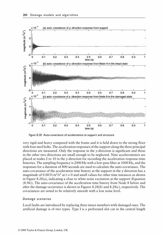
284 Damage mode ls and a lgor i thms
Figure 8.28 Auto-covariance of accelerations at support and structure
very rigid and heavy compared with the frame and it is held down to the strong floorwith four steel bolts. The acceleration responses of the support along the three principaldirections are measured. Only the response in the y-direction is significant and thosein the other two directions are small enough to be neglected. Nine accelerometers areplaced at nodes 2 to 10 in the y-direction for recording the acceleration response-timehistories. The sampling frequency is 2000 Hz with a low-pass filter at 1000 Hz, and theresponses for a duration of 800 seconds are used to calculate the auto-covariance. Theauto-covariance of the acceleration time history at the support in the y-direction has amagnitude of 0.0031 m2/s4 at t = 0 and small values for other time instances as shownin Figure 8.28(a), indicating a close to white noise excitation at the support (Equation(8.96)). The auto-covariance of the acceleration time history from Node 8 before andafter the damage occurrence is shown in Figures 8.28(b) and 8.28(c), respectively. Thecovariances are noted to be relatively smooth with a low noise level.
Damage scenar ios
Local faults are introduced by replacing three intact members with damaged ones. Theartificial damage is of two types. Type I is a perforated slot cut in the central length
© 2009 Taylor & Francis Group, London, UK
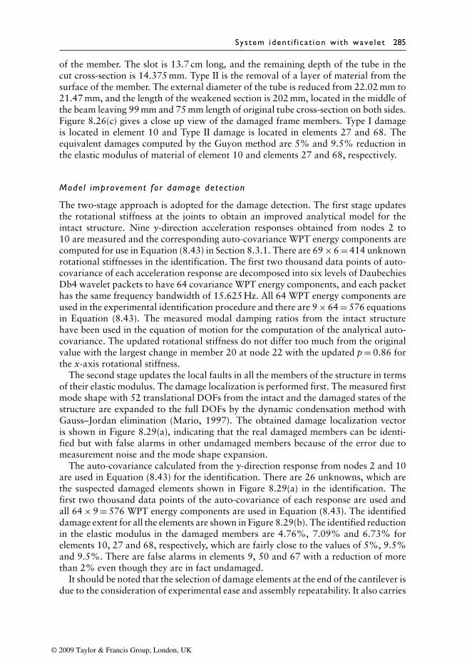
System ident i f i ca t ion wi th wave let 285
of the member. The slot is 13.7 cm long, and the remaining depth of the tube in thecut cross-section is 14.375 mm. Type II is the removal of a layer of material from thesurface of the member. The external diameter of the tube is reduced from 22.02 mm to21.47 mm, and the length of the weakened section is 202 mm, located in the middle ofthe beam leaving 99 mm and 75 mm length of original tube cross-section on both sides.Figure 8.26(c) gives a close up view of the damaged frame members. Type I damageis located in element 10 and Type II damage is located in elements 27 and 68. Theequivalent damages computed by the Guyon method are 5% and 9.5% reduction inthe elastic modulus of material of element 10 and elements 27 and 68, respectively.
Model improvement for damage detect ion
The two-stage approach is adopted for the damage detection. The first stage updatesthe rotational stiffness at the joints to obtain an improved analytical model for theintact structure. Nine y-direction acceleration responses obtained from nodes 2 to10 are measured and the corresponding auto-covariance WPT energy components arecomputed for use in Equation (8.43) in Section 8.3.1. There are 69 × 6 = 414 unknownrotational stiffnesses in the identification. The first two thousand data points of auto-covariance of each acceleration response are decomposed into six levels of DaubechiesDb4 wavelet packets to have 64 covariance WPT energy components, and each packethas the same frequency bandwidth of 15.625 Hz. All 64 WPT energy components areused in the experimental identification procedure and there are 9 × 64 = 576 equationsin Equation (8.43). The measured modal damping ratios from the intact structurehave been used in the equation of motion for the computation of the analytical auto-covariance. The updated rotational stiffness do not differ too much from the originalvalue with the largest change in member 20 at node 22 with the updated p = 0.86 forthe x-axis rotational stiffness.
The second stage updates the local faults in all the members of the structure in termsof their elastic modulus. The damage localization is performed first. The measured firstmode shape with 52 translational DOFs from the intact and the damaged states of thestructure are expanded to the full DOFs by the dynamic condensation method withGauss–Jordan elimination (Mario, 1997). The obtained damage localization vectoris shown in Figure 8.29(a), indicating that the real damaged members can be identi-fied but with false alarms in other undamaged members because of the error due tomeasurement noise and the mode shape expansion.
The auto-covariance calculated from the y-direction response from nodes 2 and 10are used in Equation (8.43) for the identification. There are 26 unknowns, which arethe suspected damaged elements shown in Figure 8.29(a) in the identification. Thefirst two thousand data points of the auto-covariance of each response are used andall 64 × 9 = 576 WPT energy components are used in Equation (8.43). The identifieddamage extent for all the elements are shown in Figure 8.29(b). The identified reductionin the elastic modulus in the damaged members are 4.76%, 7.09% and 6.73% forelements 10, 27 and 68, respectively, which are fairly close to the values of 5%, 9.5%and 9.5%. There are false alarms in elements 9, 50 and 67 with a reduction of morethan 2% even though they are in fact undamaged.
It should be noted that the selection of damage elements at the end of the cantilever isdue to the consideration of experimental ease and assembly repeatability. It also carries
© 2009 Taylor & Francis Group, London, UK
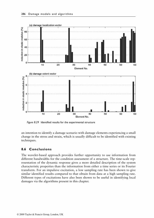
286 Damage mode ls and a lgor i thms
Figure 8.29 Identified results for the experimental structure
an intention to identify a damage scenario with damage elements experiencing a smallchange in the stress and strain, which is usually difficult to be identified with existingtechniques.
8.6 Conclusions
The wavelet-based approach provides further opportunity to use information fromdifferent bandwidths for the condition assessment of a structure. The time-scale rep-resentation of the dynamic response gives a more detailed description of the systemcharacteristic properties than the information from either a time series or its Fouriertransform. For an impulsive excitation, a low sampling rate has been shown to givesimilar identified results compared to that obtain from data at a high sampling rate.Different types of excitations have also been shown to be useful in identifying localdamages via the algorithms present in this chapter.
© 2009 Taylor & Francis Group, London, UK
Chapter 9
Uncertainty analysis
9.1 Introduction
Structural condition assessment involves many uncertainties, which come from themodelling procedure, measurements and environmental variations (Ang and Tang,1984; 2007). Ignoring the effects of these uncertainties could lead to an unsuccessfulassessment with damage undetected or intact elements identified as damaged. It isimportant to locate the sources of these uncertainties and how they evolve throughoutthe damage identification process.
Uncertainty in models and computer simulations generally arises from the measure-ment, environmental variability, parameter variability and modelling with a lack ofknowledge. Measurement variability mainly comes from experimental procedures andequipment. It includes measurement errors and data processing errors. Environmentalvariability includes the uncertainty associated with environmental variables, such astemperature, humidity, wind and traffic loads. Parameter variability is the uncertaintyassociated with the input parameters of a particular model. Modelling uncertainty, orlack of knowledge, refers to the uncertainty associated with the functional form ofthe models implemented or simplified assumptions. In summary, the uncertainties instructural condition assessment may be attributed to (Hao and Xia, 2005):
• Inaccuracy in finite element model discretization;• Uncertainties in geometry and boundary conditions;• Variations in materials properties;• Errors associated with the measured signals;• Environmental variability (such as temperature, humidity, wind and traffic).
These uncertainties can be further classified into three groups according to theirsources, namely as, the modelling, measurement and environmental uncertainties.They propagate through the damage identification process, and an integrated pro-cedure is required to estimate the probability that the failure criterion is met or notwith this effect.
Ang and Leon (2005) have tried to model and analyze these uncertainties forrisk-informed decisions, while Ellingwood (2005) reported on the state of practiceof risk-informed condition assessment of civil infrastructure for their maintenance,
© 2009 Taylor & Francis Group, London, UK

288 Damage mode ls and a lgor i thms
management (Frangopol and Liu, 2007) and safety evaluation (Liu et al., 2009a;2009b). The effect on the maintenance of civil structures (Frangopol and Messer-vey, 2009a) and the life-cycle cost estimation of deteriorating structures has also beenreported (Frangopol et al., 1997; Frangopol and Messervey, 2009b). However, theintegration of the reliability analysis with structural health monitoring has not beenattempted. The reliability analysis results of a structure are known to be a function ofthe health monitoring or condition assessment results, and yet the inclusion of sucha relationship in the reliability analysis has not been performed due to the lack ofknowledge of the uncertainty propagation in the assessment process.
The three types of uncertainties and their influence to the structural condition assess-ment are discussed in this chapter. Some of the existing approaches to formulate theireffect on the dynamic response and on the condition assessment results are also given.Finally, a box-section bridge deck structure is taken to illustrate how these uncer-tainties are considered in the integration of structural condition assessment with thesubsequent reliability analysis to yield an updated set of indices.
9.2 System uncertainties
The different stages of the computational modelling and simulation process relevantto the damage identification are depicted in Figure 9.1 (Oberkampf et al., 2002).Uncertainty is presented in all these stages, including the conceptual modelling ofthe physical system, its symbolic representation as a mathematical model and thesubsequent numerical computation and solution. In this section, some of the generalconsiderations associated with uncertainty quantification and special issues related tomodel uncertainty are discussed.
9.2.1 Modell ing uncertainty
Modelling uncertainty or uncertainty from the model can be introduced during eitherthe conceptual or the mathematical modelling processes. During the conceptual mod-elling stage, no mathematical equations are written, but the fundamental assumptionsregarding possible events and physical processes are made. All possible factors that
PhysicalSystem
ConceptualModelling
MathematicalModelling
Discretization andalgorithm selection
Computerprogramming
Numericalsolution
SolutionRepresentation
Figure 9.1 Phases of computational modelling and simulation
© 2009 Taylor & Francis Group, London, UK
Uncerta in ty ana lys i s 289
could affect the set of requirements for the modelling and simulation are considered.Also, the possible physical couplings of these factors are identified. Since it is notpossible to model complex and realistic systems at the level of elementary particles,most real-world mathematical models are comprised of a set of field equations andassociated boundary and initial conditions. These equations are approximations ofthe complicated physics of the real world. Thus, modelling uncertainty can arise fromapproximations or errors in the form of the model equations, the applied loads andthe boundary and initial conditions.
The discretization phase converts the continuum mathematics model into a dis-crete mathematics problem suitable for numerical solution. In general, a finite elementmodel is a discrete numerical model of a continuous structural system. When a finiteelement model is constructed to predict the dynamic properties of a structure, it usuallyinvolves some simplifications, where complicated parts of the structure are representedapproximately by standard elements in the model. Discretization errors are introducedwhen there is a difference between the actual dynamic properties of the system andthose predicted by the finite element model.
Methods are available for the systematic treatment of uncertainty in physical models.If the uncertainty is due to physics that are known, but not modelled, either the modelcan be revised to include these physics or an attempt can be made to characterize theuncertainty included. However, if the physics are not known, little can be done tocharacterize the accompanying uncertainty.
9.2.2 Parameter uncertainty
The parameter uncertainty refers simply to uncertainty in the input parameters of amodel. Once the form of a model has been specified by a complete set of mathematicalequations, all that remains for a complete mathematical statement of the problem isnumerical quantification of the various constants. These constants may be geometricor material properties, or they may be those that characterize the applied loads, theboundary conditions or the initial conditions. Parameter uncertainties are caused by thedifferences between the actual parameters and the analytical ones estimated from thedrawing. It is common for it to be impossible to construct a real structure exactly thesame way as it is designed. Parameter uncertainty is perhaps the most widely studiedtype of uncertainty. The characterization of the effect of this type of uncertainty on themodel prediction is analyzed by a wide variety of techniques, such as sensitivity anal-ysis, Monte Carlo methods, reliability-based methods, fuzzy set, interval propagationmethods and stochastic finite elements.
The parameter uncertainty can be reduced by model updating if the vibrationproperties of the real system are available. It has become an important topic in thedevelopment of model updating algorithms and many procedures for model verifica-tion or validation.
9.2.3 Measurement and environmental uncertainty
Measurement uncertainty refers to the uncertainties arising from the measurementprocess itself. The inherent variability may come from noise in the measurement processdue to factors such as thermal instability, internal or external electromagnetic fieldsand the quantization error. Error and potential uncertainty may arise from electrical
© 2009 Taylor & Francis Group, London, UK
290 Damage mode ls and a lgor i thms
bias and the gain errors of the signal processing tools. Measurement uncertainty formsa significant part of the overall uncertainty. In many situations, measured data aretaken as the indisputable truth. This is obviously not correct because the accuracyof measurements depends on the characteristics of the hardware, and on the physicalor empirical models underlying the design of the data collection system. An honestquantification of measurement uncertainty is crucial to a meaningful characterizationof uncertainty as a whole.
The treatment of measurement uncertainties has a history almost as long as measure-ment itself. The most common method of treating bias, gain and temporal or frequencyerrors is by calibrating each piece of measurement equipment with respect to knownstandards. Less common is the calibration of the entire measurement system.
Environmental variability includes the uncertainty associated with environmentalvariables such as temperature and humidity. For the purpose of this discussion, it alsoincludes measurement errors, data processing errors and uncertainty with the descrip-tion of loads and boundary conditions associated with environmental variables. Mostenvironmental variability can be dealt with as a parametric uncertainty. Uncertaintythat cannot be modelled easily is generally accounted for by perturbing the availableinformation with a random process as shown in the following sections.
9.3 System identification with parameter uncertainty
The sources of uncertainty were studied in Section 9.2., These mainly come from themodelling procedure and measurement and environmental variations. Another task inthe uncertainty analysis is to study the effect of uncertainty on the condition assessmentand to estimate the statistical distribution or bounds of the identified results, which istermed the uncertainty propagation in system identification.
While there are many studies on the effect of uncertainty in the modal analysis, relia-bility analysis, model updating, etc., other researchers try to quantify the uncertainty inidentified modal parameters using the singular value decomposition technique (SVD)(Ruotolo and Surace, 1999) or using the principal component analysis of a matrix ofestimated features (Kullaa, 2002). This is successful as the damage features are outliers.However, it only works well when the SVD of the data matrix from intact observa-tions can be computed. In another application of the SVD, the parameter variations aredecomposed into principal components that are weighted based on the sensitivity of theperformance matrix to the parameter variations (Vanlanduit et al., 2005). Parameterbounds in the form of an interval model are generated and each interval corresponds toone identified bounded uncertainty parameter with its associated principal direction.
Two commonly used numerical approaches to study the uncertainty propagation arethe Monte Carlo simulation and the perturbation method. In the Monte Carlo simu-lation, a large number of samples with a given probability distribution are generated(Kottegoda and Rosso, 1997). A specified process is then applied to these data samplesto estimate the statistics of the output. The Bootstrap method (Efron and Tibshirani,1994) is somewhat similar to Monte Carlo simulation. It has the advantage of requir-ing no assumptions about the distribution functions or covariance matrices. However,this technique requires that every data sample be reused in the generation of the nextsample. An alterative approach is the perturbation method. This approach expandsa nonlinear function with a truncated Taylor series expansion at a known point and
© 2009 Taylor & Francis Group, London, UK
Uncerta in ty ana lys i s 291
then proceeds to the approximation of the moments of solutions from the expansion.Certainly, the Monte Carlo simulation method can be combined with the perturbationmethod for the uncertainty propagation study. The minimum variance method mak-ing use of the above combined techniques was first studied by Collins et al. (1974)to obtain the statistical properties of updating parameters. Beck and his co-workers(Beck and Katafygiotis, 1998; Katafygiotis and Beck, 1998) have also reformulated thismethod in a more general framework where the Bayesian method is used to minimizethe variance of the updated structural parameters.
9.3.1 Monte Carlo simulation
The Monte Carlo simulation has been widely used in statistical analysis. Differentsets of input data are obtained based on the statistics and an assumed probabilitydistribution of the input data. A specified process is then applied to the simulateddata to obtain the output for each set of inputs, from which, the distribution andthe interval bounds of the output can be estimated. It is particularly useful when aclosed-form solution is impossible or very difficult to obtain.
To perform a Monte Carlo simulation, one needs to specify the probability distri-bution of the variables involved, which must be known or assumed. The generationof outcomes from a prescribed probability distribution is a fundamental task in thesimulation process. In designing the Monte Carlo simulation, one must determinehow many simulations are required to assess the system behaviour with the error ofassessment decreasing as n−1/2, where n is the number of simulations. To estimatethe probability, p, of an event within 100 ε% (where ε is the acceptable tolerance,0 ≤ ε≤ 1) of its true value with 100(1 −α)% confidence, n must satisfy (Kottegodaand Rosso, 1997)
n ≥ z2α/2(1 − p)/ε2p (9.1)
where zα/2 denotes a standard normal variate that is exceeded with the probability ofα/2. Since n is a function of p, which is unknown before the experiment is performed,the value of p must be estimated before the experiment.
While increasing the sample size is one way to reduce the standard error of a MonteCarlo analysis, the fact of doing so can be computationally expensive. A better solutionis to employ some technique of variance reduction based on the properties of corre-lated samples. Standard techniques of variance reduction including antithetic variates,control variates, importance sampling and stratified sampling (Kottegoda and Rosso,1997) may be used for this purpose.
9.3.2 Integrated perturbed and Bayesian method
Before the integrated perturbed and Bayesian methods are introduced, the perturbationmethod is first presented. The identified distribution of updated parameters is thencombined with the prior distributions of updated parameters via Bayesian updating toachieve the posterior distributions of the updated parameters.
The perturbation method generally takes a small disturbance into the undisturbedsystem. Here the uncertainty is taken as a perturbation from the noise-free data. It isclosely related to the Taylor series expansion and is useful when the uncertainty level
© 2009 Taylor & Francis Group, London, UK
292 Damage mode ls and a lgor i thms
is not high, such that the first few terms can approximate the important features of thesolution and the remaining ones can be truncated. In model updating, the relationshipbetween the measured vibration characteristics and the structural parameters can beexpressed as:
{e} = [S]{�α} (9.2)
where {e} is the modal data change vector containing the differences between the eigen-values and mode shapes at the corresponding measured degrees-of-freedom (DOF) ofthe structure before and after updating; {�α} = {α} − {α} is the vector of parameterchange, where {α} and {α} are structural elemental parameters of the initial and updatedfinite element model; and [S] is the corresponding sensitivity matrix.
Different accuracies of approximation to the solution statistics can be achieveddepending on the order of truncation of the Taylor series expansion used in the per-turbation method. In practical applications, either the first-order, second momentapproach or the second-order, second moment approach can be used to approximatethe solution moments. The first-order, second moment approach approximates thenonlinear function with a linear expansion at a point of the space of the random vari-ables, and the obtained mean and covariance are of first-order accuracy. The limitationsof the first-order perturbation method are that uncertainties must not be too largeand that the nonlinearity is not significant. Quadratic accuracy can be achieved byapproaching the nonlinear function with a second-order Taylor series expansion asillustrated with the following example.
Applying the perturbation technique, Equation (9.2) can be expanded as a second-order Taylor series in terms of the uncertainty, Xi, (Liu, 1995), which is taken as theselected uncertainty here.
[S] = [S]0 +N∑
i=1
∂[S]∂Xi
Xi + 12
N∑i=1
N∑j=1
∂2[S]∂Xi ∂Xj
XiXj (9.3)
{�α} = {�α}0 +N∑
i=1
∂{�α}∂Xi
Xi + 12
N∑i=1
N∑j=1
∂2{�α}∂Xi ∂Xj
XiXj (9.4)
{e} = {e}0 +N∑
i=1
∂{e}∂Xi
Xi + 12
N∑i=1
N∑j=1
∂2{e}∂Xi ∂Xj
XiXj (9.5)
It is noted that superscript ‘0’ represents the respective noise-free value. Substitutingthe above equations into Equation (9.2) and comparing the terms of 1, Xi, Xi and Xj,then {�α}0, ∂{�α}/∂Xi, ∂2{�α}/∂Xi ∂Xj (i, j = 1, 2, . . . , N) can be solved as follows
{�α}0 = ([S]0)+{e}0 (9.6)
∂{�α}∂Xi
= ([S]0)+(∂{e}∂Xi
− ∂[S]∂Xi
{�α}0)
(9.7)
© 2009 Taylor & Francis Group, London, UK
Uncerta in ty ana lys i s 293
∂2{�α}∂Xi ∂Xj
= ([S]0)+(∂2{e}∂Xi ∂Xj
− ∂2[S]∂Xi ∂Xj
{�α}0 − 2∂[S]∂Xi
∂{�α}∂Xj
)(9.8)
where + denotes the general inverse of a matrix. Noting that E(Xi) = 0 and the meanvalues and covariance matrix of {�α} approximating the nonlinear function can beobtained from Equation (9.4) as follows
E({�α}) = E({�α}0) + 12
N∑i=1
∂2{�α}∂2Xi
Cov(Xi, Xi) (9.9)
[Cov(�α,�α)] =[∂{�α}∂{X}
][Cov(X, X)]
[∂{�α}∂{X}
]T
(9.10)
In practice, structural parameters are estimated from sources such as the designdrawing, which are subjected to uncertainties. Such an estimate of structural param-eters is termed as prior information. The Bayesian approach is very useful when oneis faced with two sets of uncertain information and one needs to know which set tobelieve. Both the prior information and the newly obtained information are used toaccount for the relative uncertainty associated with each other. The newly obtainedinformation can be derived from the perturbation approach. The prior informationis given by the structural analysis prior to the testing of a structure. The Bayesianapproach is then applied to obtain a new (posterior) distribution with the aboveinformation.
Assuming there is a random structural parameter, α, with a probability densityfunction, f1(α), the identified probability density function is obtained as f2(α) from theabove perturbation method. The posterior probability density function of the structuralparameter can be expressed as the following with the Bayesian probabilistic framework(Sohn and Law, 1997; Vanik et al., 2000),
f (α) = kL(α)f2(α) (9.11)
where L(α) represents the likelihood function and k is the normalized constant.For the case where the probability density functions of both f1(α) and f2(α) are
normally distributed, the posterior distribution function of the structural parameter,f (α), also complies with a normal distribution, where the mean and standard deviationare obtained as (Hua et al., 2007)
µ = µ1σ22 + µ2σ
21
σ21 + σ2
2
(9.12)
σ =√σ2
1σ22
σ21 + σ2
2
(9.13)
where µ1 and µ2 are the means of prior and the identified distribution function,respectively; and σ1 and σ2 are the corresponding standard deviations, respectively.
© 2009 Taylor & Francis Group, London, UK
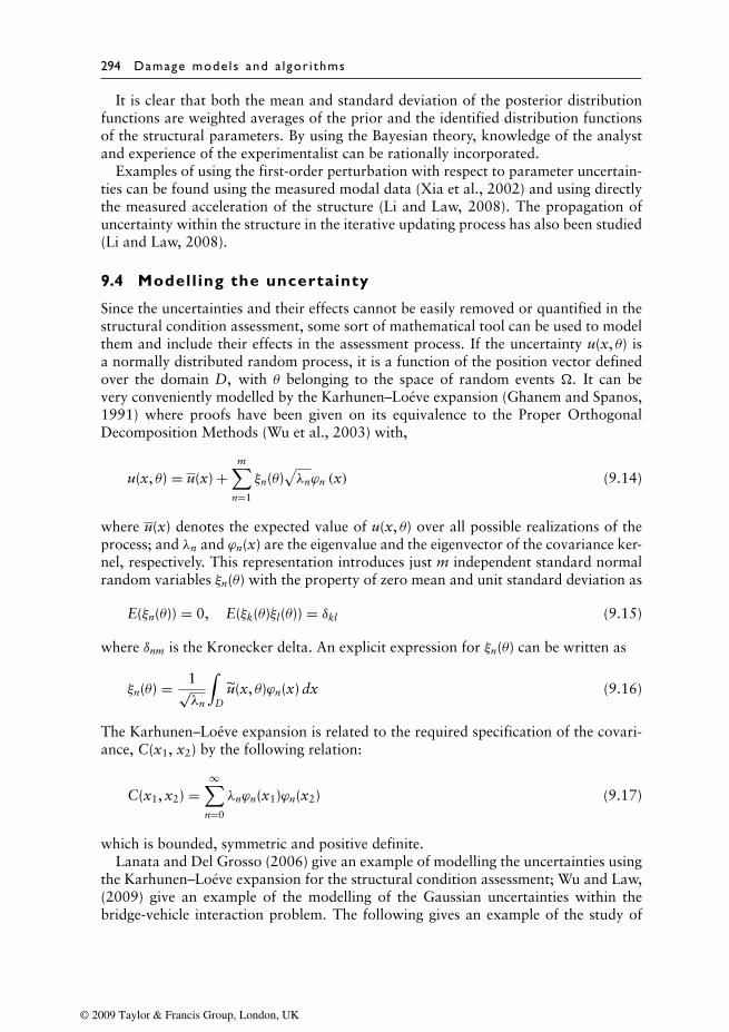
294 Damage mode ls and a lgor i thms
It is clear that both the mean and standard deviation of the posterior distributionfunctions are weighted averages of the prior and the identified distribution functionsof the structural parameters. By using the Bayesian theory, knowledge of the analystand experience of the experimentalist can be rationally incorporated.
Examples of using the first-order perturbation with respect to parameter uncertain-ties can be found using the measured modal data (Xia et al., 2002) and using directlythe measured acceleration of the structure (Li and Law, 2008). The propagation ofuncertainty within the structure in the iterative updating process has also been studied(Li and Law, 2008).
9.4 Modelling the uncertainty
Since the uncertainties and their effects cannot be easily removed or quantified in thestructural condition assessment, some sort of mathematical tool can be used to modelthem and include their effects in the assessment process. If the uncertainty u(x, θ) isa normally distributed random process, it is a function of the position vector definedover the domain D, with θ belonging to the space of random events �. It can bevery conveniently modelled by the Karhunen–Loéve expansion (Ghanem and Spanos,1991) where proofs have been given on its equivalence to the Proper OrthogonalDecomposition Methods (Wu et al., 2003) with,
u(x, θ) = u(x) +m∑
n=1
ξn(θ)√λnϕn (x) (9.14)
where u(x) denotes the expected value of u(x, θ) over all possible realizations of theprocess; and λn and ϕn(x) are the eigenvalue and the eigenvector of the covariance ker-nel, respectively. This representation introduces just m independent standard normalrandom variables ξn(θ) with the property of zero mean and unit standard deviation as
E(ξn(θ)) = 0, E(ξk(θ)ξl(θ)) = δkl (9.15)
where δnm is the Kronecker delta. An explicit expression for ξn(θ) can be written as
ξn(θ) = 1√λn
∫D
u(x, θ)ϕn(x) dx (9.16)
The Karhunen–Loéve expansion is related to the required specification of the covari-ance, C(x1, x2) by the following relation:
C(x1, x2) =∞∑
n=0
λnϕn(x1)ϕn(x2) (9.17)
which is bounded, symmetric and positive definite.Lanata and Del Grosso (2006) give an example of modelling the uncertainties using
the Karhunen–Loéve expansion for the structural condition assessment; Wu and Law,(2009) give an example of the modelling of the Gaussian uncertainties within thebridge-vehicle interaction problem. The following gives an example of the study of
© 2009 Taylor & Francis Group, London, UK
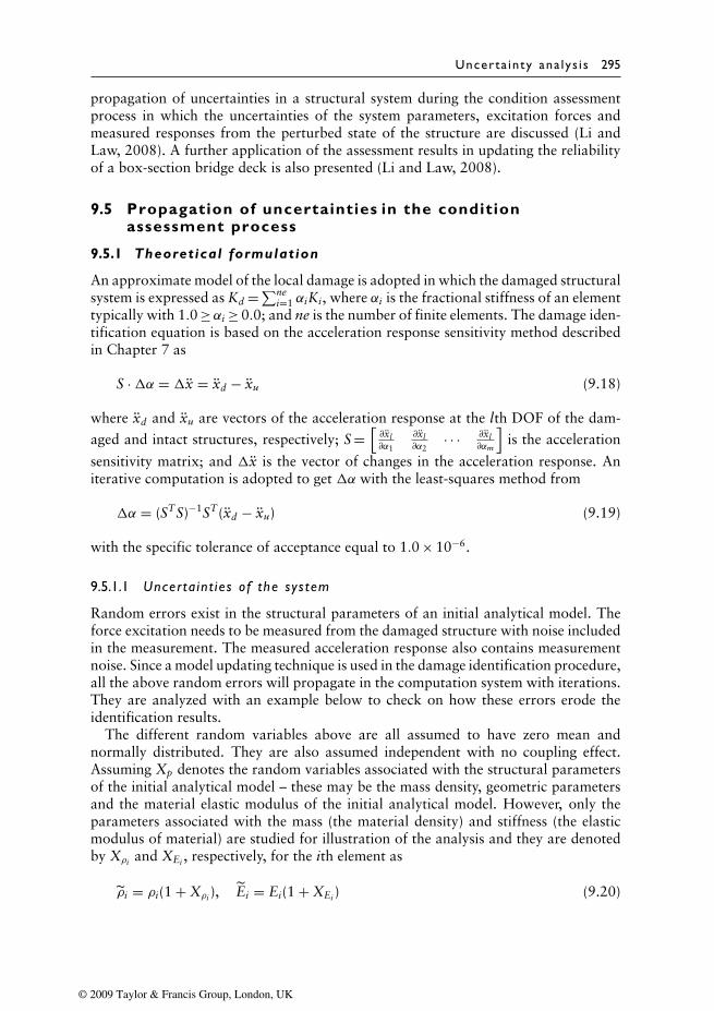
Uncerta in ty ana lys i s 295
propagation of uncertainties in a structural system during the condition assessmentprocess in which the uncertainties of the system parameters, excitation forces andmeasured responses from the perturbed state of the structure are discussed (Li andLaw, 2008). A further application of the assessment results in updating the reliabilityof a box-section bridge deck is also presented (Li and Law, 2008).
9.5 Propagation of uncertainties in the conditionassessment process
9.5.1 Theoretical formulation
An approximate model of the local damage is adopted in which the damaged structuralsystem is expressed as Kd =∑ne
i=1 αiKi, where αi is the fractional stiffness of an elementtypically with 1.0 ≥αi ≥ 0.0; and ne is the number of finite elements. The damage iden-tification equation is based on the acceleration response sensitivity method describedin Chapter 7 as
S ·�α = �x = xd − xu (9.18)
where xd and xu are vectors of the acceleration response at the lth DOF of the dam-
aged and intact structures, respectively; S =[∂xl∂α1
∂xl∂α2
· · · ∂xl∂αm
]is the acceleration
sensitivity matrix; and �x is the vector of changes in the acceleration response. Aniterative computation is adopted to get �α with the least-squares method from
�α = (STS)−1ST (xd − xu) (9.19)
with the specific tolerance of acceptance equal to 1.0 × 10⁻⁶.
9.5.1.1 Uncer ta in t ies of the sys tem
Random errors exist in the structural parameters of an initial analytical model. Theforce excitation needs to be measured from the damaged structure with noise includedin the measurement. The measured acceleration response also contains measurementnoise. Since a model updating technique is used in the damage identification procedure,all the above random errors will propagate in the computation system with iterations.They are analyzed with an example below to check on how these errors erode theidentification results.
The different random variables above are all assumed to have zero mean andnormally distributed. They are also assumed independent with no coupling effect.Assuming Xp denotes the random variables associated with the structural parametersof the initial analytical model – these may be the mass density, geometric parametersand the material elastic modulus of the initial analytical model. However, only theparameters associated with the mass (the material density) and stiffness (the elasticmodulus of material) are studied for illustration of the analysis and they are denotedby Xρi and XEi , respectively, for the ith element as
ρi = ρi(1 + Xρi ), Ei = Ei(1 + XEi ) (9.20)
© 2009 Taylor & Francis Group, London, UK
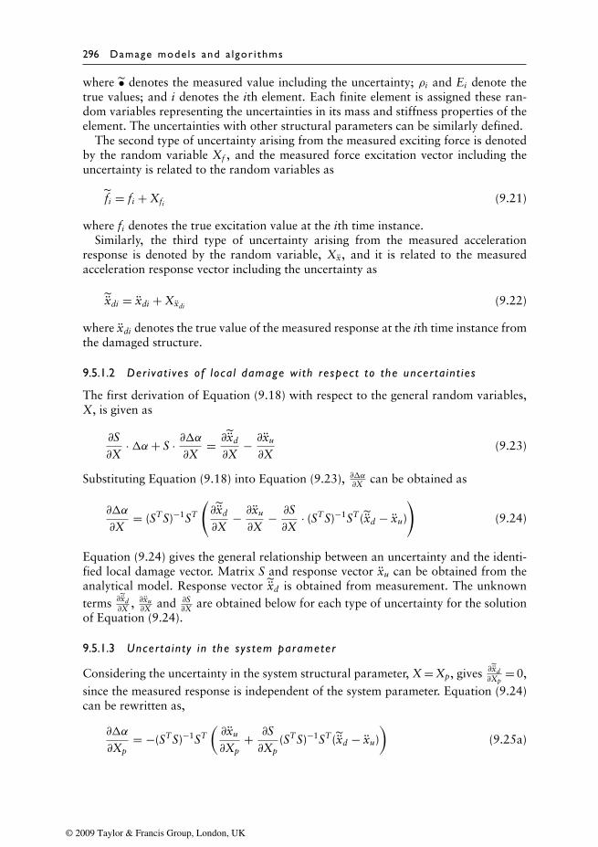
296 Damage mode ls and a lgor i thms
where • denotes the measured value including the uncertainty; ρi and Ei denote thetrue values; and i denotes the ith element. Each finite element is assigned these ran-dom variables representing the uncertainties in its mass and stiffness properties of theelement. The uncertainties with other structural parameters can be similarly defined.
The second type of uncertainty arising from the measured exciting force is denotedby the random variable Xf , and the measured force excitation vector including theuncertainty is related to the random variables as
fi = fi + Xfi (9.21)
where fi denotes the true excitation value at the ith time instance.Similarly, the third type of uncertainty arising from the measured acceleration
response is denoted by the random variable, Xx, and it is related to the measuredacceleration response vector including the uncertainty as
˜xdi = xdi + Xxdi (9.22)
where xdi denotes the true value of the measured response at the ith time instance fromthe damaged structure.
9.5.1.2 Der ivat i ves of loca l damage wi th respect to the uncer ta in t ies
The first derivation of Equation (9.18) with respect to the general random variables,X, is given as
∂S∂X
·�α+ S · ∂�α∂X
= ∂xd
∂X− ∂xu
∂X(9.23)
Substituting Equation (9.18) into Equation (9.23), ∂�α∂X can be obtained as
∂�α
∂X= (STS)−1ST
(∂xd
∂X− ∂xu
∂X− ∂S∂X
· (STS)−1ST (xd − xu)
)(9.24)
Equation (9.24) gives the general relationship between an uncertainty and the identi-fied local damage vector. Matrix S and response vector xu can be obtained from theanalytical model. Response vector ˜xd is obtained from measurement. The unknownterms ∂xd
∂X , ∂xu∂X and ∂S
∂X are obtained below for each type of uncertainty for the solutionof Equation (9.24).
9.5.1.3 Uncer ta in ty in the sys tem parameter
Considering the uncertainty in the system structural parameter, X = Xp, gives ∂xd∂Xp
= 0,since the measured response is independent of the system parameter. Equation (9.24)can be rewritten as,
∂�α
∂Xp= −(STS)−1ST
(∂xu
∂Xp+ ∂S∂Xp
(STS)−1ST (xd − xu))
(9.25a)
© 2009 Taylor & Francis Group, London, UK
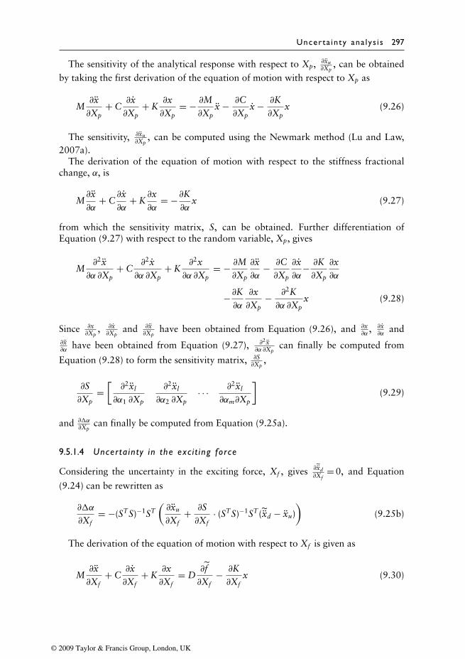
Uncerta in ty ana lys i s 297
The sensitivity of the analytical response with respect to Xp, ∂xu∂Xp
, can be obtainedby taking the first derivation of the equation of motion with respect to Xp as
M∂x∂Xp
+ C∂x∂Xp
+ K∂x∂Xp
= − ∂M∂Xp
x − ∂C∂Xp
x − ∂K∂Xp
x (9.26)
The sensitivity, ∂xu∂Xp
, can be computed using the Newmark method (Lu and Law,2007a).
The derivation of the equation of motion with respect to the stiffness fractionalchange, α, is
M∂x∂α
+ C∂x∂α
+ K∂x∂α
= −∂K∂α
x (9.27)
from which the sensitivity matrix, S, can be obtained. Further differentiation ofEquation (9.27) with respect to the random variable, Xp, gives
M∂2x∂α ∂Xp
+ C∂2x∂α ∂Xp
+ K∂2x∂α ∂Xp
= − ∂M∂Xp
∂x∂α
− ∂C∂Xp
∂x∂α
− ∂K∂Xp
∂x∂α
−∂K∂α
∂x∂Xp
− ∂2K∂α ∂Xp
x (9.28)
Since ∂x∂Xp
, ∂x∂Xp
and ∂x∂Xp
have been obtained from Equation (9.26), and ∂x∂α
, ∂x∂α
and∂x∂α
have been obtained from Equation (9.27), ∂2x∂α ∂Xp
can finally be computed from
Equation (9.28) to form the sensitivity matrix, ∂S∂Xp
,
∂S∂Xp
=[∂2xl
∂α1 ∂Xp
∂2xl
∂α2 ∂Xp· · · ∂2xl
∂αm∂Xp
](9.29)
and ∂�α∂Xp
can finally be computed from Equation (9.25a).
9.5.1.4 Uncer ta in ty in the exc i t ing force
Considering the uncertainty in the exciting force, Xf , gives ∂xd∂Xf
= 0, and Equation
(9.24) can be rewritten as
∂�α
∂Xf= −(STS)−1ST
(∂xu
∂Xf+ ∂S∂Xf
· (STS)−1ST (xd − xu))
(9.25b)
The derivation of the equation of motion with respect to Xf is given as
M∂x∂Xf
+ C∂x∂Xf
+ K∂x∂Xf
= D∂f∂Xf
− ∂K∂Xf
x (9.30)
© 2009 Taylor & Francis Group, London, UK
298 Damage mode ls and a lgor i thms
Thus, from Equation (9.21)
∂f (t)∂Xfi
= [0 · · · 0 1 0 · · · 0]T (9.31)
where only the ith component of the vector is one with zeros in all the other com-ponents. For the initial analytical model, ∂K
∂Xf= 0, but in the updated analytical
model, the effect of force uncertainty has propagated in the updated model withα=α0 +�α1 +�α2 + . . . , where α is the updated vector of the fractional parame-ter; α0 is the initial vector of the fractional parameter; and �αi is the vector of thefractional parameter change identified after the ith iteration. Since the initial vector ofthe fractional parameter is independent of the force uncertainty, ∂α
0
∂Xf= 0, and
∂K∂Xf
= ∂K∂α
∂α
∂Xf= ∂K∂α
∂(α0 +�α1 +�α2 + · · · )∂Xf
= ∂K∂α
(∂α0
∂Xf+ ∂(�α
1)∂Xf
+ ∂(�α2)
∂Xf+ · · ·
)= ∂K∂α
(∂(�α1)∂Xf
+ ∂(�α2)
∂Xf+ · · ·
)(9.32)
Since ∂�αi
∂Xf= 0, then ∂K
∂Xf= 0. The sensitivity, ∂xu
∂Xf, can be computed from Equations
(9.30) to (9.32) by the Newmark method.Differentiating Equation (9.27) with respect to the random variable, Xf , gives
M∂2x∂α ∂Xf
+ C∂2x∂α ∂Xf
+ K∂2x∂α ∂Xf
= −∂K∂α
∂x∂Xf
− ∂K∂Xf
∂x∂α
− ∂2K∂Xf ∂α
x (9.33)
which is similar to Equation (9.24). ∂S∂Xf
can then be computed from Equations (9.30)
to (9.33) using the Newmark method and the sensitivity, ∂�α∂Xf
, can then be obtained
from Equation (9.25b). The effect of the uncertainty is seen to be propagating withiterations in the structural system through Equations (9.32), (9.33) and (9.25b).
9.5.1.5 Uncer ta in ty in the st ruct ura l response
The sensitivity of �α with respect to the random variable Xx can also be obtainedsimilar to that for the structural parameters. Since xu and S are not related to Xx inthe initial analytical model, ∂xu
∂Xx= 0 and ∂S
∂Xx= 0. Equation (9.24) then gives
∂�α
∂Xx= (STS)−1ST ∂xd
∂Xx(9.34a)
© 2009 Taylor & Francis Group, London, UK
Uncerta in ty ana lys i s 299
However, in the updated analytical model, both xu and S are related to Xx with theuncertainties propagated in the system. The derivation of the equation of motion withrespect to Xx gives
M∂x∂Xx
+ C∂x∂Xx
+ K∂x∂Xx
= − ∂K∂Xx
x (9.35)
The sensitivities, ∂x∂Xx
and ∂x∂Xx
, can be obtained from Equation (9.35) using the New-mark method. ∂K
∂Xxcan be obtained in a manner similar to Equation (9.32). The
derivation of Equation (9.26) with respect to Xx gives
M∂2x∂α ∂Xx
+ C∂2x∂α ∂Xx
+ K∂2x∂α ∂Xx
= −∂K∂α
∂x∂Xx
− ∂2K∂α ∂Xx
x − ∂K∂Xx
∂x∂α
(9.36)
and ∂�α∂Xx
can be written as follows, incorporating Equations (9.35) and (9.36) as
∂�α
∂Xx= (STS)−1ST
(∂xd
∂Xx− ∂xu
∂Xx− ∂S∂Xx
(STS)−1ST (xd − xu)
)(9.34b)
Equation (9.32) is obtained from Equation (9.22) as
∂xd(t)∂Xx
= [0 · · · 0 1 0 · · · 0]T (9.37)
and the sensitivity, ∂�α∂Xx
, is obtained from Equations (9.34) and (9.37). The effect of theuncertainty is seen to be propagating with iterations in the structural system througha modified version of Equation (9.32) and Equations (9.35) and (9.34b).
In summary, the vector of sensitivity, ∂�α∂X , can be obtained from Equations (9.25a),
(9.25b) and (9.24) as
∂�α
∂X=[∂�α
∂Xp
∂�α
∂Xf
∂�α
∂Xx
](9.38)
9.5.1.6 Stat i s t i ca l character i s t i cs o f the damage vector
The mean value of the damage vector, �α, can be obtained directly from Equation(9.19) as
E(�α) = (STS)−1ST (xd − xu) (9.39)
since the uncertainties considered in this paper are with zero means. The damage vector,�α, can be regarded as a function of the random variables, and it can be expressed asa truncated second-order Taylor series as
�α(X) = �α(0) +mt∑i=1
∂�α(0)∂Xi
Xi + 12
mt∑i=1
mt∑j=1
∂2�α(0)∂Xi ∂Xj
XiXj (9.40)
© 2009 Taylor & Francis Group, London, UK
300 Damage mode ls and a lgor i thms
where Xi and Xj denote the ith and jth variables, respectively; and mt is the numberof random variables in the statistical analysis. The covariance matrix of �α may beobtained as (Papadopoulos and Garcia, 1998)
[cov(�α,�α)]m×m ≈[∂�α
∂X
]m×mt
[cov(X, X)]mt×mt
[∂�α
∂X
]T
m×mt
(9.41)
Since the random variables, Xi and Xj (i = j), are assumed independent,
[cov(X, X)]mt×mt =
cov(X1, X1) 0 · · · 0
0 cov(X2, X2) · · · 0· · · · · · · · · · · ·0 0 · · · cov(Xmt, Xmt)
(9.42)
It is noted that the covariance matrix of the random variables, cov(X, X), can becomputed separately.
Random variables, Xp, are usually assumed to take the following form as
Xp = Ep · N (9.43)
where Ep is a constant defining the level of variation and N is a normally distributedvector with zero mean and unit standard deviation. This gives
cov(Xp, Xp) =
(Ep)2 0 · · · 0
0 (Ep)2 · · · 0· · · · · · · · · · · ·0 0 · · · (Ep)2
(9.44)
For the random variable, Xf , with the excitation force, is modelled as
Xf = Ep · N · σ f (9.45)
where f is the vector of polluted force excitation; and σ f is the standard deviation ofthe measured force time history. Thus,
cov(Xf , Xf ) =
(Ep)2 · var(f ) 0 · · · 0
0 (Ep)2 · var(f ) · · · 0· · · · · · · · · · · ·0 0 · · · (Ep)2 · var(f )
(9.46)
where var(•) is the variance of the time history. For the random variables, Xx, whichare the measurement noise in the acceleration response
Xx = Ep · N · σ˜xd(9.47)
© 2009 Taylor & Francis Group, London, UK
Uncerta in ty ana lys i s 301
Then the covariance of Xx is
cov(Xx, Xx) =
(Ep)2 · var(xd) 0 · · · 0
0 (Ep)2 · var(xd) · · · 0· · · · · · · · · · · ·0 0 · · · (Ep)2 · var(xd)
(9.48)
Hence, Equations (9.44), (9.46) and (9.48) give the covariance matrix of all the randomvariables in the present study.
9.5.1.7 Stat i s t i ca l ana lys i s in damage ident i f i cat ion
Statistical analysis of the identified results can be performed using Equations (9.39)and (9.41). Assuming that α0 corresponds to the set of initial parameter changes in theanalytical model, the updated set of parameter changes, α1, will be given as
α1 = α0 +�α1 (9.49)
with an expectation value of
E(α1) = E(α0) + E(�α1) (9.50)
and a covariance of
[cov(α1,α1)]m×m = cov(α0 +�α1,α0 +�α1)
= cov(α0,α0) + cov(α0,�α1) + cov(�α1,α0) + cov(�α1,�α1)
(9.51)
It is noted that Equations (9.50) and (9.51) will remain valid during the whole processof convergence of the identified results.
9.5.2 Numerical example
9.5.2.1 The st ructure
The three-dimensional five-bay cantilever steel frame structure studied in Sections7.4 and 8.5 is shown in Figure 9.2. The finite element model consists of 37 three-dimensional Euler beam elements and 17 nodes. A summary of the main material andgeometrical properties of the members of the frame structure is given in Table 7.1. Thesupport conditions and dynamic characteristics of the structure are referred to Section8.5.2.1.
A sinusoidal excitation is applied onto the structure at the 8th node in the z-directionwith an amplitude of 3 N and at a frequency of 30 Hz. The acceleration responsecomputed at the 5th node in the z-direction is taken as the ‘measured’ response andthe first 500 data points are used to identify the damage. The sampling frequency is2000 Hz. A damage case with 5% and 10% reduction of the flexural stiffness in the7th member and the 26th member, respectively, is studied. The effect of each type ofuncertainty on the damage identification is discussed below.
© 2009 Taylor & Francis Group, London, UK
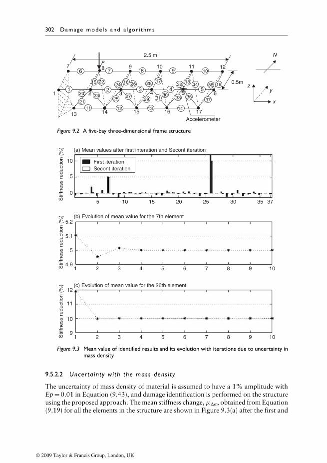
302 Damage mode ls and a lgor i thms
x
zy
1 2 3 4 5 6
7 8 9 10 11 12
13 14 15 16 17
1 2 3 4 5
7 8 9 106
11 12 13 14
15 16 17 18 19
20
21
22
23
24 26
25 27
28
2930
31
32
33
34
35
36
37
2.5 m
0.5m
N
Accelerometer
F
Figure 9.2 A five-bay three-dimensional frame structure
0
5.2
5.1
5
4.9
12
11
10
9
5
10
5
First iteration
(a) Mean values after first interation and Secont iteration
(b) Evolution of mean value for the 7th element
(c) Evolution of mean value for the 26th element
Secont iteration
10 15 20 25 30 35 37
1 2 3 4 5 6 7 8 9 10
1 2 3Stif
fnes
s re
duct
ion
(%)
Stif
fnes
s re
duct
ion
(%)
Stif
fnes
s re
duct
ion
(%)
4 5 6 7 8 9 10
Figure 9.3 Mean value of identified results and its evolution with iterations due to uncertainty inmass density
9.5.2.2 Uncer ta in ty wi th the mass dens i t y
The uncertainty of mass density of material is assumed to have a 1% amplitude withEp = 0.01 in Equation (9.43), and damage identification is performed on the structureusing the proposed approach. The mean stiffness change, µ�α, obtained from Equation(9.19) for all the elements in the structure are shown in Figure 9.3(a) after the first and
© 2009 Taylor & Francis Group, London, UK
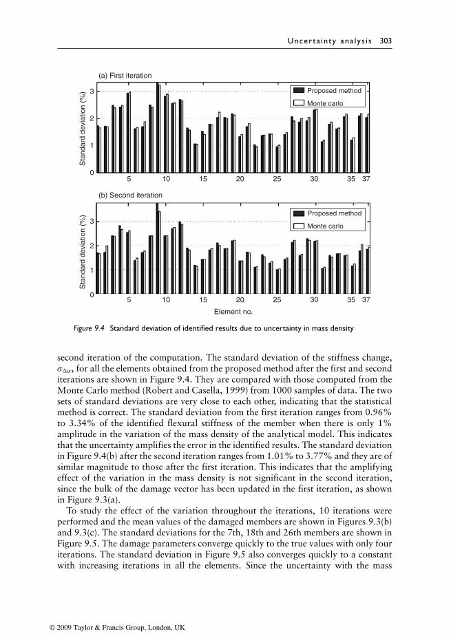
Uncerta in ty ana lys i s 303
0
1
2
3
0
1
2
3
5 10 15 20 25 30 35 37
5 10 15 20
Element no.
25 30 35 37
(a) First iteration
(b) Second iteration
Proposed method
Monte carlo
Proposed method
Monte carlo
Sta
ndar
d de
viat
ion
(%)
Sta
ndar
d de
viat
ion
(%)
Figure 9.4 Standard deviation of identified results due to uncertainty in mass density
second iteration of the computation. The standard deviation of the stiffness change,σ�α, for all the elements obtained from the proposed method after the first and seconditerations are shown in Figure 9.4. They are compared with those computed from theMonte Carlo method (Robert and Casella, 1999) from 1000 samples of data. The twosets of standard deviations are very close to each other, indicating that the statisticalmethod is correct. The standard deviation from the first iteration ranges from 0.96%to 3.34% of the identified flexural stiffness of the member when there is only 1%amplitude in the variation of the mass density of the analytical model. This indicatesthat the uncertainty amplifies the error in the identified results. The standard deviationin Figure 9.4(b) after the second iteration ranges from 1.01% to 3.77% and they are ofsimilar magnitude to those after the first iteration. This indicates that the amplifyingeffect of the variation in the mass density is not significant in the second iteration,since the bulk of the damage vector has been updated in the first iteration, as shownin Figure 9.3(a).
To study the effect of the variation throughout the iterations, 10 iterations wereperformed and the mean values of the damaged members are shown in Figures 9.3(b)and 9.3(c). The standard deviations for the 7th, 18th and 26th members are shown inFigure 9.5. The damage parameters converge quickly to the true values with only fouriterations. The standard deviation in Figure 9.5 also converges quickly to a constantwith increasing iterations in all the elements. Since the uncertainty with the mass
© 2009 Taylor & Francis Group, London, UK
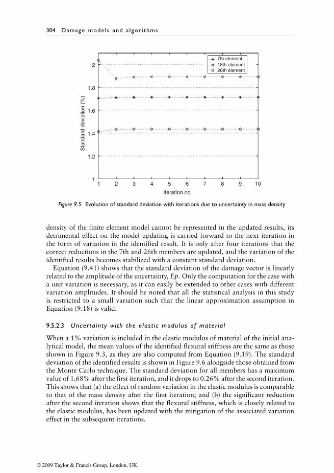
304 Damage mode ls and a lgor i thms
11 2
Sta
ndar
d de
viat
ion
(%)
3 4 5
Iteration no.
6 7 8 9 10
1.2
1.4
1.6
1.8
27th element18th element26th element
Figure 9.5 Evolution of standard deviation with iterations due to uncertainty in mass density
density of the finite element model cannot be represented in the updated results, itsdetrimental effect on the model updating is carried forward to the next iteration inthe form of variation in the identified result. It is only after four iterations that thecorrect reductions in the 7th and 26th members are updated, and the variation of theidentified results becomes stabilized with a constant standard deviation.
Equation (9.41) shows that the standard deviation of the damage vector is linearlyrelated to the amplitude of the uncertainty, Ep. Only the computation for the case witha unit variation is necessary, as it can easily be extended to other cases with differentvariation amplitudes. It should be noted that all the statistical analysis in this studyis restricted to a small variation such that the linear approximation assumption inEquation (9.18) is valid.
9.5.2.3 Uncer ta in ty wi th the e las t i c modu lus of mater ia l
When a 1% variation is included in the elastic modulus of material of the initial ana-lytical model, the mean values of the identified flexural stiffness are the same as thoseshown in Figure 9.3, as they are also computed from Equation (9.19). The standarddeviation of the identified results is shown in Figure 9.6 alongside those obtained fromthe Monte Carlo technique. The standard deviation for all members has a maximumvalue of 1.68% after the first iteration, and it drops to 0.26% after the second iteration.This shows that (a) the effect of random variation in the elastic modulus is comparableto that of the mass density after the first iteration; and (b) the significant reductionafter the second iteration shows that the flexural stiffness, which is closely related tothe elastic modulus, has been updated with the mitigation of the associated variationeffect in the subsequent iterations.
© 2009 Taylor & Francis Group, London, UK
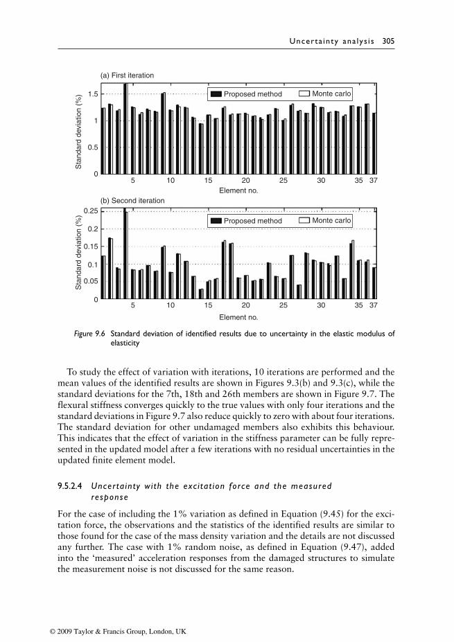
Uncerta in ty ana lys i s 305
05 10 15
(b) Second iteration
(a) First iteration
Proposed method Monte carlo
20
Element no.
Element no.25 30 35 37
5 10 15
Sta
ndar
d de
viat
ion
(%)
Sta
ndar
d de
viat
ion
(%)
20 25 30 35 37
0.5
1
1.5
0
0.05
0.1
0.15
0.2
0.25Proposed method Monte carlo
Figure 9.6 Standard deviation of identified results due to uncertainty in the elastic modulus ofelasticity
To study the effect of variation with iterations, 10 iterations are performed and themean values of the identified results are shown in Figures 9.3(b) and 9.3(c), while thestandard deviations for the 7th, 18th and 26th members are shown in Figure 9.7. Theflexural stiffness converges quickly to the true values with only four iterations and thestandard deviations in Figure 9.7 also reduce quickly to zero with about four iterations.The standard deviation for other undamaged members also exhibits this behaviour.This indicates that the effect of variation in the stiffness parameter can be fully repre-sented in the updated model after a few iterations with no residual uncertainties in theupdated finite element model.
9.5.2.4 Uncer ta in ty wi th the exc i ta t ion force and the measuredresponse
For the case of including the 1% variation as defined in Equation (9.45) for the exci-tation force, the observations and the statistics of the identified results are similar tothose found for the case of the mass density variation and the details are not discussedany further. The case with 1% random noise, as defined in Equation (9.47), addedinto the ‘measured’ acceleration responses from the damaged structures to simulatethe measurement noise is not discussed for the same reason.
© 2009 Taylor & Francis Group, London, UK
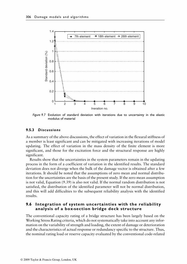
306 Damage mode ls and a lgor i thms
01 2 3 4 5 6
Ineration no.
Sta
ndar
d de
viat
ion
(%)
7 8 9 10
0.2
0.4
0.6
0.8
1
1.2
1.4
7th element 18th element 26th element
Figure 9.7 Evolution of standard deviation with iterations due to uncertainty in the elasticmodulus of material
9.5.3 Discussions
As a summary of the above discussions, the effect of variation in the flexural stiffness ofa member is least significant and can be mitigated with increasing iterations of modelupdating. The effect of variation in the mass density of the finite element is moresignificant, and those for the excitation force and the structural response are highlysignificant.
Results show that the uncertainties in the system parameters remain in the updatingprocess in the form of a coefficient of variation in the identified results. The standarddeviation does not diverge when the bulk of the damage vector is obtained after a fewiterations. It should be noted that the assumptions of zero mean and normal distribu-tion for the uncertainties are the basis of the present study. If the zero mean assumptionis not valid, Equation (9.39) is also not valid. If the normal random distribution is notsatisfied, the distribution of the identified parameter will not be normal distribution,and this will add difficulties to the subsequent reliability analysis with the identifiedresults.
9.6 Integration of system uncertainties with the reliabil ityanalysis of a box-section bridge deck structure
The conventional capacity rating of a bridge structure has been largely based on theWorking Stress Rating criteria, which do not systematically take into account any infor-mation on the variability of strength and loading, the extent of damage or deteriorationand the characteristics of actual response or redundancy specific to the structure. Thus,the nominal rating load or reserve capacity evaluated by the conventional code-related
© 2009 Taylor & Francis Group, London, UK
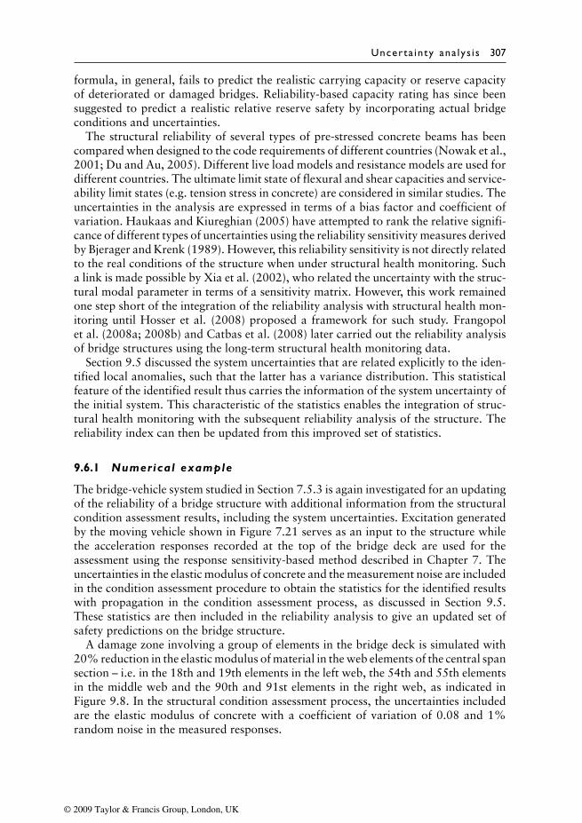
Uncerta in ty ana lys i s 307
formula, in general, fails to predict the realistic carrying capacity or reserve capacityof deteriorated or damaged bridges. Reliability-based capacity rating has since beensuggested to predict a realistic relative reserve safety by incorporating actual bridgeconditions and uncertainties.
The structural reliability of several types of pre-stressed concrete beams has beencompared when designed to the code requirements of different countries (Nowak et al.,2001; Du and Au, 2005). Different live load models and resistance models are used fordifferent countries. The ultimate limit state of flexural and shear capacities and service-ability limit states (e.g. tension stress in concrete) are considered in similar studies. Theuncertainties in the analysis are expressed in terms of a bias factor and coefficient ofvariation. Haukaas and Kiureghian (2005) have attempted to rank the relative signifi-cance of different types of uncertainties using the reliability sensitivity measures derivedby Bjerager and Krenk (1989). However, this reliability sensitivity is not directly relatedto the real conditions of the structure when under structural health monitoring. Sucha link is made possible by Xia et al. (2002), who related the uncertainty with the struc-tural modal parameter in terms of a sensitivity matrix. However, this work remainedone step short of the integration of the reliability analysis with structural health mon-itoring until Hosser et al. (2008) proposed a framework for such study. Frangopolet al. (2008a; 2008b) and Catbas et al. (2008) later carried out the reliability analysisof bridge structures using the long-term structural health monitoring data.
Section 9.5 discussed the system uncertainties that are related explicitly to the iden-tified local anomalies, such that the latter has a variance distribution. This statisticalfeature of the identified result thus carries the information of the system uncertainty ofthe initial system. This characteristic of the statistics enables the integration of struc-tural health monitoring with the subsequent reliability analysis of the structure. Thereliability index can then be updated from this improved set of statistics.
9.6.1 Numerical example
The bridge-vehicle system studied in Section 7.5.3 is again investigated for an updatingof the reliability of a bridge structure with additional information from the structuralcondition assessment results, including the system uncertainties. Excitation generatedby the moving vehicle shown in Figure 7.21 serves as an input to the structure whilethe acceleration responses recorded at the top of the bridge deck are used for theassessment using the response sensitivity-based method described in Chapter 7. Theuncertainties in the elastic modulus of concrete and the measurement noise are includedin the condition assessment procedure to obtain the statistics for the identified resultswith propagation in the condition assessment process, as discussed in Section 9.5.These statistics are then included in the reliability analysis to give an updated set ofsafety predictions on the bridge structure.
A damage zone involving a group of elements in the bridge deck is simulated with20% reduction in the elastic modulus of material in the web elements of the central spansection – i.e. in the 18th and 19th elements in the left web, the 54th and 55th elementsin the middle web and the 90th and 91st elements in the right web, as indicated inFigure 9.8. In the structural condition assessment process, the uncertainties includedare the elastic modulus of concrete with a coefficient of variation of 0.08 and 1%random noise in the measured responses.
© 2009 Taylor & Francis Group, London, UK

308 Damage mode ls and a lgor i thms
27 sensors
Bearing:
Fixed
Guided
Free
Path of wheels
Damaged webelements 90 and 91
Damaged webelements 18 and 19
Damaged webelements 54 and 55
Figure 9.8 Plan of bridge and sensor configuration
Damage detection is performed with the two-axle three-dimensional vehicle crossingthe bridge deck along the travel path shown in Figure 9.8. It is noted that the vehicletravels on top of the left web. The velocity of the vehicle is 20 m/s and the samplingrate is 100 Hz. Road surface roughness Class C (ISO, 1995) is included in the analysis.It is noted that Class C road roughness corresponds to the average road pavementconditions, which is modelled as a noise distribution in the measured responses inaddition to the 1% measurement noise. The parameters of the vehicle are taken fromMarchesiello et al. (1999) with a mass of 17000 kg.
9.6.2 Condit ion assessment
Only the 108 web elements are included as candidates in the assessment. Each inter-action force is modelled with 600 terms in its orthogonal expansions. Since theinteraction forces of the four wheels and local damages in the structural elementsare all unknowns, acceleration responses recorded at 27 locations on top of the deckas shown in Figure 9.8 are used in the identification to ensure that the identifica-tion equation is over-determined. The vehicle passes over the deck in 3.75 seconds,and there are 375 time instances with the vehicle moving on top of the bridge deck.There are 27 × 375 = 10125 equations for solving the 4 × 600 + 108 = 2508 numberof unknowns in the inverse problem.
The interaction forces calculated are kept as reference for comparison, while thecalculated responses of the deck are used for the inverse identification. Figures 9.9and 9.10 give the identified interaction force-time histories and the identified localdamages in the bridge deck. The identified wheel-load-time histories from ‘unpol-luted’ measured responses overlap with the true values, and the identified results frommeasurement with 1% noise are very accurate with a small relative error less than5%. Table 9.1 gives the associated information for convergence. There are some falsepositives in elements adjacent to the damages in Figure 9.10.
Figure 9.11 shows the coefficient of variation (COV) of the elastic constant in allthe web elements obtained after three iterations using the true or identified interactionforces with a COV of 0.08 in the elastic modulus and 1% noise in the measured
© 2009 Taylor & Francis Group, London, UK
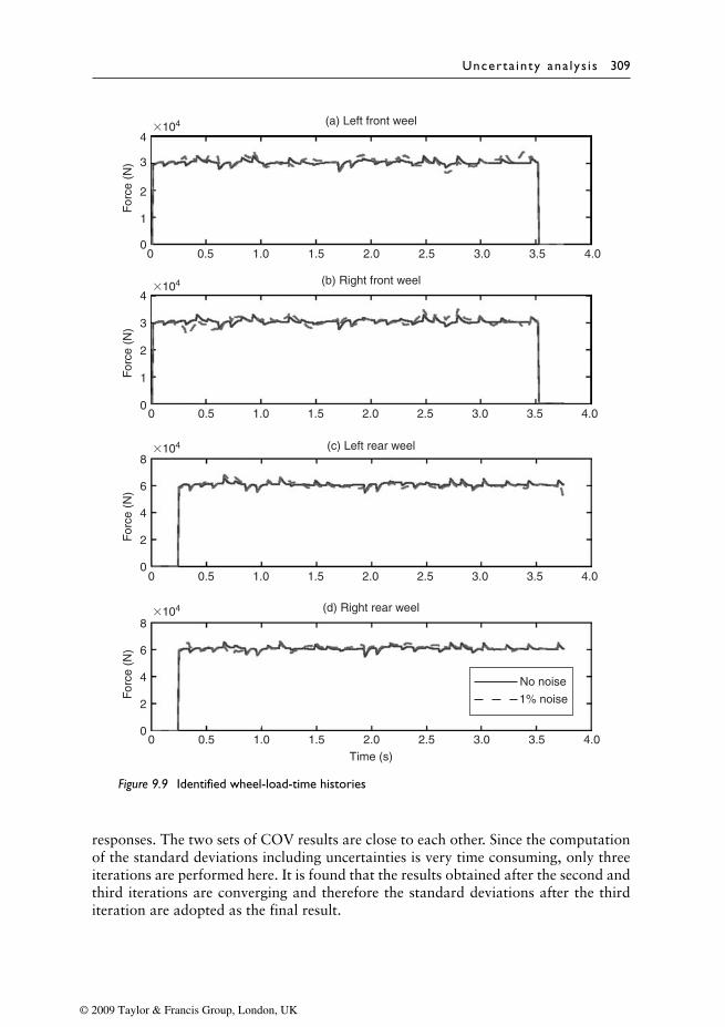
Uncerta in ty ana lys i s 309
00 0.5
(a) Left front weel
(c) Left rear weel
(d) Right rear weel
(b) Right front weel
For
ce (
N)
For
ce (
N)
For
ce (
N)
For
ce (
N)
1.0 1.5 2.0 2.5 3.0 3.5 4.0
0 0.5 1.0 1.5 2.0 2.5 3.0 3.5 4.0
0 0.5 1.0 1.5 2.0 2.5 3.0 3.5 4.0
0 0.5 1.0 1.5 2.0Time (s)
No noise
1% noise
2.5 3.0 3.5 4.0
1
2
3
4
0
1
2
3
4
0
2
4
6
8
0
2
4
6
8�104
�104
�104
�104
Figure 9.9 Identified wheel-load-time histories
responses. The two sets of COV results are close to each other. Since the computationof the standard deviations including uncertainties is very time consuming, only threeiterations are performed here. It is found that the results obtained after the second andthird iterations are converging and therefore the standard deviations after the thirditeration are adopted as the final result.
© 2009 Taylor & Francis Group, London, UK
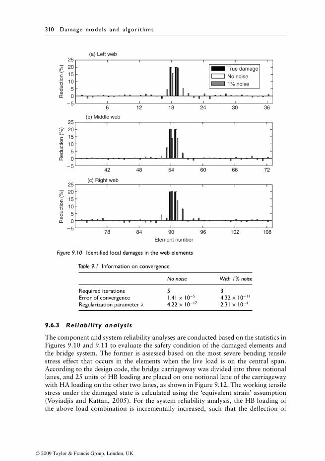
310 Damage mode ls and a lgor i thms
0
6
(a) Left web
(b) Middle web
(c) Right web
12 18 24 30
True damage
No noise1% noise
36
42 48 54 60 66 72
78 84 90
Element number
96 102 108
Red
uctio
n (%
)
5
�5
10152025
0Red
uctio
n (%
)
5
�5
10152025
0Red
uctio
n (%
)
5
�5
10152025
Figure 9.10 Identified local damages in the web elements
Table 9.1 Information on convergence
No noise With 1% noise
Required iterations 5 3Error of convergence 1.41 × 10⁻⁵ 4.32 × 10⁻¹¹
Regularization parameter λ 4.22 × 10⁻¹⁷ 2.31 × 10⁻⁴
9.6.3 Reliabi l i ty analysis
The component and system reliability analyses are conducted based on the statistics inFigures 9.10 and 9.11 to evaluate the safety condition of the damaged elements andthe bridge system. The former is assessed based on the most severe bending tensilestress effect that occurs in the elements when the live load is on the central span.According to the design code, the bridge carriageway was divided into three notionallanes, and 25 units of HB loading are placed on one notional lane of the carriagewaywith HA loading on the other two lanes, as shown in Figure 9.12. The working tensilestress under the damaged state is calculated using the ‘equivalent strain’ assumption(Voyiadjis and Kattan, 2005). For the system reliability analysis, the HB loading ofthe above load combination is incrementally increased, such that the deflection of
© 2009 Taylor & Francis Group, London, UK
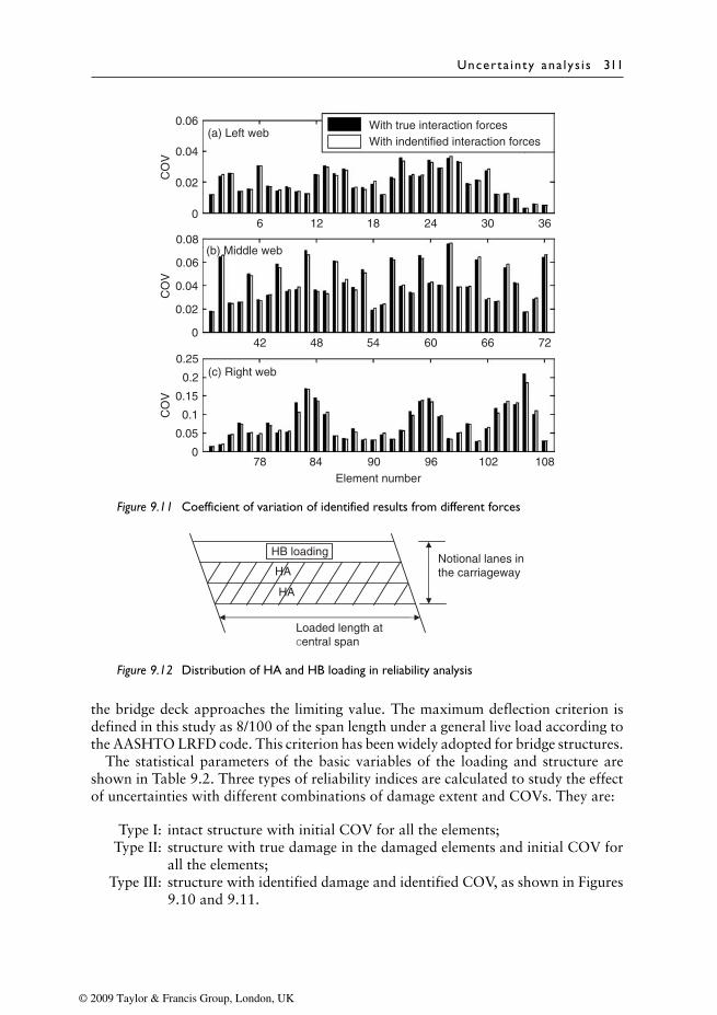
Uncerta in ty ana lys i s 311
With true interaction forcesWith indentified interaction forces
(a) Left web
Element number78
6 12
CO
VC
OV
CO
V
18 24 30 36
42 48 54 60 66 72
84 90 96 102 108
0.06
0.04
0.02
0
0.06
0.08
0.04
0.02
0
0.2
0.25
0.15
0.1
0.05
0
(b) Middle web
(c) Right web
Figure 9.11 Coefficient of variation of identified results from different forces
HB loadingNotional lanes inthe carriagewayHA
HA
Loaded length at central span
Figure 9.12 Distribution of HA and HB loading in reliability analysis
the bridge deck approaches the limiting value. The maximum deflection criterion isdefined in this study as 8/100 of the span length under a general live load according tothe AASHTO LRFD code. This criterion has been widely adopted for bridge structures.
The statistical parameters of the basic variables of the loading and structure areshown in Table 9.2. Three types of reliability indices are calculated to study the effectof uncertainties with different combinations of damage extent and COVs. They are:
Type I: intact structure with initial COV for all the elements;Type II: structure with true damage in the damaged elements and initial COV for
all the elements;Type III: structure with identified damage and identified COV, as shown in Figures
9.10 and 9.11.
© 2009 Taylor & Francis Group, London, UK

312 Damage mode ls and a lgor i thms
Table 9.2 Statistical parameters of basic variables in reliability analysis
Variable Bias factor Coefficient of variation Distribution type
Dead load, D1 1.03 0.08 NormalDead load, D2 1.05 0.10 NormalDead load, D3 1.0 0.25 NormalLive load 1.15 0.18 Type I Extreme
value DistributionPre-stress – new structure 0.97 0.04 Normal
(age< 5 years)Pre-stress – old structure 0.85 0.12 Normal
(age> 30 years)Area of pre-stress strands 1.0 0.0125 NormalTensile strength of concrete (ft) 1.0 0.23 NormalModulus of elasticity 1.0 0.08 NormalDimensions (thickness) 1.0 0.05 NormalModel coefficient 0.945 0.03 Normal
Table 9.3 Reliability index
Intact with True damage with Identified damageinitial COV initial COV with identified COV(Type I) (Type II) (Type III)
Component reliability index 18th 1.268 0.876 1.05019th 2.481 2.124 2.12854th 2.069 1.747 1.88155th 2.736 2.420 2.52690th 2.814 2.367 2.39791st 3.723 3.517 3.687
System reliability index 4.953 4.909 4.901
The Type I index gives the baseline before the damage occurrence and is the set ofindices corresponding to the design stage. The Type II index is associated with thedamage occurrence, but without the uncertainty effect from the condition assessment.This is the conventional reliability index computed from an estimated damage pattern.The Type III index is associated with the assessment results incorporating the prop-agation of uncertainty in the structure. This is the set of updated reliability indicesincorporating the effect from the structural condition assessment.
The component and system reliability indices are computed and they are shown inTable 9.3. The HB loading is placed approximately on top of the left web (Figure 9.8)creating high tensile stresses in elements 18 and 19 compared to other elements and theoriginal component reliability indices (Type I) are smaller than the others. The effectof local damage reduces the corresponding Type II and Type III indices. When thestatistics of the identified damages are further included in the analysis, the componentreliability indices (Type III) have a notable difference compared with those of TypeII. (It cannot, however, be concluded that the Type III component reliability indices
© 2009 Taylor & Francis Group, London, UK
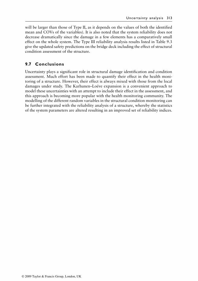
Uncerta in ty ana lys i s 313
will be larger than those of Type II, as it depends on the values of both the identifiedmean and COVs of the variables). It is also noted that the system reliability does notdecrease dramatically since the damage in a few elements has a comparatively smalleffect on the whole system. The Type III reliability analysis results listed in Table 9.3give the updated safety predictions on the bridge deck including the effect of structuralcondition assessment of the structure.
9.7 Conclusions
Uncertainty plays a significant role in structural damage identification and conditionassessment. Much effort has been made to quantify their effect in the health moni-toring of a structure. However, their effect is always mixed with those from the localdamages under study. The Karhunen–Loéve expansion is a convenient approach tomodel these uncertainties with an attempt to include their effect in the assessment, andthis approach is becoming more popular with the health monitoring community. Themodelling of the different random variables in the structural condition monitoring canbe further integrated with the reliability analysis of a structure, whereby the statisticsof the system parameters are altered resulting in an improved set of reliability indices.
© 2009 Taylor & Francis Group, London, UK
References
Abraham, M.A., Park, S.Y. and Stubbs, N. (1995) Loss of prestress prediction on nondestructivedamage location algorithms. SPIE, Smart Structures and Materials, 2456: 60–67.
Abramovich, H. (1992) Natural frequencies of Timoshenko beams under compressive axialloads. Journal of Sound and Vibration, 157(1): 183–189.
Ahmadian, H., Mottershead, J.E. and Friswell, M.I. (1998) Regularization methods for finiteelement model updating. Mechanical Systems and Signal Processing, 12(1): 47–64.
Andelfinger, U. and Ramm, E. (1992) An Assessment of Hybrid-mixed Four Node Shell Ele-ments. Nonlinear Analysis of Shells by Finite Elements. Edited by F.G. Rammerstorfer.CISM Courses and Lectures No. 328. International Centre for Mechanical Sciences.Springer-Verlag.
Ang, A.H-S. and De Leon, D. (2005) Modeling and analysis of uncertainties for risk-informeddecisions in infrastructure engineering. Structure and Infrastructure Engineering, 1(1), 19–32.Taylor & Francis.
Ang, A.H-S. and Tang, W.H. (1984) Probability Concepts in Engineering Planning and DesignVolume II. New York: John Wiley & Sons.
Ang, A.H-S. and Tang, W.H. (2007) Probability Concepts in Engineering Planning and DesignVolume II, 2nd ed. New York: Wiley.
Bagarello, F. (1995) Multiplication of distribution in one dimension: possible approaches andapplications to δ-function and its derivatives. Journal of Mathematic Analysis and Application,196(3): 885–901.
Bakhtiari-Nejad, F., Rahai, A. and Esfandiari, A. (2005) A structural damage detection methodusing static noisy data. Engineering Structures, 27(12): 1784–1793.
Banan, M.R. and Hjelmstad, K.D. (1994) Parameter estimation of structures from staticresponse. I. Computational aspects. Journal of Structural Engineering ASCE, 120(11):3243–3258.
Barbero, E.J. and Reddy, J.N. (1991) Modelling of delamination in composite laminates usinga layer-wise plate theory. International Journal of Solids and Structure, 28(3): 373–388.
Baschmid, A., Dizua, G. and Pizzigoni, B. (1984) The influence of unbalance on cracked rotors.Proceedings of the International Conference on Vibration of Rotating Machinery, 193–198.
Beck, J.L. and Katafygiotis, L.S. (1998) Updating models and their uncertainties. I: Bayesianstatistical frameworks. Journal of Engineering Mechanics ASCE, 124(4): 455–461.
Bendat, J.S. and Piersol, A.G. (1980) Engineering Applications of Correlation and SpectralAnalysis. New York: John Wiley.
Berman, A. and Flannely, W.G. (1971) Theory of incomplete models of dynamic structures.AIAA Journal, 9(8): 1481–1487.
Bjerager, P. and Krenk, S. (1989) Parametric sensitivity in first order reliability theory. Journalof Engineering Mechanics ASCE, 115(7): 1577–1582.
© 2009 Taylor & Francis Group, London, UK
316 References
Blair, M.A., Camino, T.S. and Dickens, J.M. (1991) An iterative approach to a reduced massmatrix. Proceedings of the 8th International Modal Analysis Conference, Florence, Italy,510–515.
Briggs, J.C. and Tse, M.K. (1992) Impact force identification using extracted modal parametersand pattern matching. International Journal of Impact Engineering, 12(3): 361–372.
British Standard Institution. (1990) British Standard-Structural Use of Steelwork in Building.BS5950.
Buda, G. and Caddemi, S. (2007) Identification of concentrated damages in Euler-Bernoullibeams under static loads. Journal of Engineering Mechanics ASCE, 133(8): 942–956.
Bui, H.D. (1994) Inverse problems in engineering mechanics. Proceedings of the Second Inter-national Symposium on Inverse Problems—ISIP ’94, Paris, France, 2–4 November 1994.Rotterdam; Brookfield, Vt.: A.A. Balkema.
Caddemi, S. and Greco, A. (2006) The influence of instrumental errors on the static iden-tification of damage parameters for elastic beams. Computers and Structures, 84(26–27):1696–1708.
Catbas, F.N., Susoy, M. and Frangopol, D.M. (2008) Structural health monitoring and reli-ability estimation: long span truss bridge application with environmental monitoring data.Engineering Structures, 30(9): 2347–2359.
Cawley, P. and Adams, R.D. (1979) The location of defects in structures from measurement ofnatural frequencies. Journal of Strain Analysis, 14: 49–57.
Chan, H.C., Cheung, Y.K. and Huang, Y.P. (1992) Crack analysis of reinforced concrete tensionmembers. Journal of Structural Engineering ASCE, 118(8): 2118–2132.
Chan, H.C., Cheung, Y.K. and Huang, Y.P. (1993) Analytical crack model for reinforced-concrete structures. Journal of Structural Engineering ASCE, 119(5): 1339–1357.
Chan, S.L. (1994) Vibration and modal analysis of steel frames with semi-rigid connections.Engineering Structures, 16(1): 25–31.
Chan, S.L. and Chui, P.P.T. (2000) Non-linear Static and Cyclic Analysis of Steel Frames withSemi-rigid Connections. Elsevier.
Chan, S.L. and Zhou, Z.H. (1998) On the development of a robust element for second-ordernon-linear integrated design and analysis. Journal of Constructional Steel Research, 47(1–2):169–190.
Chang, C.C. and Chen, L.W. (2003) Vibration damage detection of a Timoshenko beam byspatial wavelet based approach. Applied Acoustics, 64(12): 1217–1240.
Chaudhry, Z. and Ganino, A.J. (1994) Damage detection using neutral network: an initial exper-imental study on debonded beams. Journal of Intelligent Material Systems and Structures,5(4): 585–589.
Chen, J.C. and Garba, J.A. (1980) Analytical model improvement using modal testing results.AIAA Journal, 18(6): 684–690.
Chen, J. and Li, J. (2004) Simultaneous identification of structural parameters and input timehistory from output-only measurements. Computational Mechanics, 33(5): 365–374.
Chen, W.F., Takanashi, K., Nakashima, M. and White, D. (1998) US-Japan seminar on inno-vations in stability concepts and methods for seismic design in structural steel. EngineeringStructures, 20(4–6): 239–569.
Choi, C.K., Kim, K.H. and Hong, H.S. (2002) Spline finite strip analysis of prestressed concretebox-girder bridges. Engineering Structures, 24(12): 1575–1586.
Chui, P.P.T. and Chan, S.L. (1997) Vibration and deflection characteristics of semi-rigid jointedframes. Engineering Structures, 19(12): 1001–1010.
Coifman, R.R. and Wickerhauser, M.V. (1992) Entropy-based algorithms for best basis selection.IEEE Transactions on Information Theory, 38(2): 713–718.
Collins, J.D. and Hart, G.C., Hasselman, T.K. and Kennedt, B. (1974) Statistical identificationof structures. AIAA Journal, 12: 185–190.
© 2009 Taylor & Francis Group, London, UK
References 317
Cornwell, P., Doebling, S.W. and Farrar, C.R. (1999) Application of the strain energy dam-age detection method to plate-like structures. Journal of Sound and Vibration, 224(2):359–374.
Dallard, P., Fitzpatrick, A.J., Flint, A., Bourva, S.L.e, Low, A., Ridsdill, R.M. and Willford, M.(2001) The London Millennium Footbridge. The Structural Engineer, 79(22): 17–33.
Daubechies, I. (1988) Orthonormal bases of compactly supported wavelets. Communicationson Pure and Applied Mathematics, 41(7): 909–996.
Daubechies, I. (1992) Ten Lectures on Wavelets. Philadelphia, PA: SIAM.Devriendt, C. and Fontul, M. (2005) Transmissibility in coupled structures: identification of the
sufficient set of coupling forces. First International Operational Modal Analysis Conference,Copenhagen, Denmark, April, 2005. Edited by Rune Brincker and Nis Møller. Published byAalborg University: 445–453.
Diaz Valdes, S.H. and Soutis, C. (1999a) Application of the rapid frequency sweep technique fordelamination detection in composite laminates. Advanced Composite Letters, 8(1): 19–23.
Diaz Valdes, S.H. and Soutis, C. (1999b) Delamination detection in composite laminates fromvariations of their modal characteristics. Journal of Sound and Vibration, 228(1): 1–9.
Dimarogonas, A.D. (1996) Vibration of cracked structures: a state of the art review. EngineeringFracture Mechanics, 55(5): 831–857.
Di Paola, M. and Bilello, C. (2004) An integral for damage identification of Euler-Bernoullibeams under static loads. Journal of Engineering Mechanics ASCE, 130(2): 225–234.
Doebling, S.W. (1995) Measurement of Structural Flexibility Matrices for Experiments withIncomplete Reciprocity. PhD Dissertation, Aerospace Engineering Sciences Dept., Universityof Colorado, Boulder, CO.
Doebling, S.W. (1996) Damage detection and model refinement using elemental stiffness per-turbations with constrained connectivity. Proceedings of the AIAA/ASME/AHS AdaptiveStructures Forum: 360–370.
Doebling, S.W., Peterson, L.D. and Alvin, K.F. (1998a) Experimental determination of localstructural stiffness by disassembly of measured flexibility matrices. Journal of Vibration andAcoustics ASME, 120(4): 949–957.
Doebling, S.W., Farrar, C.R. and Prime, M.B. (1998b) A summary review of vibration-baseddamage identification methods. Shock and Vibration Digest, 30(2): 91–105.
Douka, E., Loutridis, S. and Trochidis, A. (2003) Crack identification in beams using waveletanalysis. International Journal of Solids and Structures, 40(13): 3557–3569.
Doyle, J.F. (1994) A genetic algorithm for determining the location of structural impacts.Experimental Mechanics, 34(1): 37–44.
Du, J.S. and Au, F.T.K. (2005) Deterministic and reliability analysis of prestressed concretebridge girders: comparison of the Chinese, Hong Kong and AASHTO LRFD Codes. StructuralSafety, 27(3): 230–245.
Efron, B. and Tibshirani, R.J. (1994) An Introduction to the Bootstrap. New York: Chapman &Hall.
Ellingwood, B.R. (2005) Risk-informed condition assessment of civil infrastructure: state ofpractice and research needs, Structure and Infrastructure Engineering, 1(1), 7–18. Taylor &Francis.
Farrar, C.R., Duffey, T.A., Doebling, S.W. and Nix, D.A. (1999) A statistical pattern recog-nition paradigm for vibration-based structural health monitoring. Proceedings of the 2ndInternational Workshop on Structural Health Monitoring, 764–773.
Figueiras, J.A. and Póvoas, H.H.C.F. (1994) Modelling of prestress in non-linear analysis ofconcrete structures. Computers & Structures, 53(1): 173–187.
Frangopol, D.M. and Liu, M. (2007) Maintenance and management of civil infrastructurebased on condition, safety, optimization, and life-cycle cost. Structure and InfrastructureEngineering, 3(1), 29–41.
© 2009 Taylor & Francis Group, London, UK
318 References
Frangopol, D.M., Lin, K-Y. and Estes, A.C. (1997) Life-cycle cost design of deterioratingstructures. Journal of Structural Engineering ASCE, 123(10), 1390–1401.
Frangopol, D.M., and Messervey, T.B. (2009a). “Maintenance principles for civil structures,’’Chapter 89 in Encyclopedia of Structural Health Monitoring, C. Boller, F-K. Chang, andY. Fujino, eds., John Wiley & Sons Ltd, Chicester, UK, Vol. 4, 1533–1562.
Frangopol, D.M., and Messervey, T.B. (2009b). “Life-cycle cost and performance prediction:Role of structural health monitoring,’’ in Frontier Technologies for Infrastructures Engineer-ing, Chapter 16, S-S, Chen and A.H-S. Ang, eds., CRC Press, Taylor & Francis, London,361–381.
Frangopol, D.M., Strauss, A. and Kim, S.Y. (2008a) Bridge reliability assessment based onmonitoring. Journal of Bridge Engineering ASCE, 13(3): 258–270.
Frangopol, D. M., Strauss, A., and Kim, S. (2008b). “Use of monitoring extreme data for theperformance prediction of structures: General approach’’ Engineering Structures, Elsevier, 30(12), 3644–3653.
Fregolent, A., D’ambrogio, W., Salvini, P. and Sestieri, A. (1996) Regularisation techniquesfor dynamic model updating using input residual. Inverse Problems in Engineering, 2:171–200.
Friswell, M.I. and Mottershead, J.E. (1995) Finite Element Model Updating in StructuralDynamics. Kluwer Academic Publisher: Dordrecht, The Netherlands.
Friswell, M.I. and Mottershead, J.E. (1996) Identification in engineering systems: Proceedingsof the conference held at Swansea, March 1996. Swansea [England]: University of WalesSwansea.
Friswell, M.I., Garvey, S.D. and Penny, J.E.T. (1995) Model reduction using dynamic and iteratedIRS techniques. Journal of Sound and Vibration, 186(2): 311–323.
Friswell, M.I., Mottershead, J.E. and Lees, A.W. (1999) Identification in engineering systems:proceedings of the second international conference held in Swansea, March 1999. Publisher[Swansea : University of Wales].
Fox, R.L. and Kappor, M.R. (1968) Rates of change of eigenvalues and eigenvectors. AIAAJournal, 6(12): 2426–2429.
Gao, L. and Haldar, A. (1995) Nonlinear seismic analysis of space structures with partiallyrestrained connections. Microcomputer Civil Engineering, 10(1): 27–37.
Ge, L. and Soong, T.T. (1998) Damage identification through regularization method. I: Theory.Journal of Engineering Mechanics ASCE, 124(1): 103–108.
Gentile, A. and Messina, A. (2003) On the continuous wavelet transforms applied to discretevibrational data for detecting open cracks in damaged beams. International Journal of Solidsand Structures, 40(2): 295–315.
Ghanem, R. and Spanos, P.D. (1991) Stochastic Finite Elements: A Spectral Approach, NewYork: Springer-Verlag, Inc.
Gladwell, G.M.L. and Ahmadian, H. (1995) Generic element matrices suitable for finite elementmodel updating. Mechanical Systems and Signal Processing, 9(6): 601–614.
Griffin, S.F. and Sun, T.C. (1991) Health monitoring of dumb and smart structures. Proceedingsof the 28th Annual Meeting of SES, November 6–8, Gainsville, Florida.
Grigorian, C.E., Yang, T.S. and Popov, E.P. (1992) Slotted bolted connection energy dissipators.Report of National Science Foundation, University of California, Berkeley.
Goldfarb, D. and Idnani, A. (1983) A numerically stable dual method for solving strictly convexquadratic problems. Mathematical Programming, 27(1): 1–33.
Golub, G.H. (1996) Matrix Computation. Johns Hopkins University Press.Golub, G.H., Heath, M. and Wahba, G. (1979) Generalized cross-validation as a method for
choosing a good ridge parameter. Technometrics, 27(2): 215–223.Gontier, C. and Bensaibi, M. (1995) Time domain identification of a substructure from in situ
analysis of the whole structure. Mechanical Systems and Signal Processing, 9(4): 379–396.
© 2009 Taylor & Francis Group, London, UK
References 319
Gordis, J.H. (1992) An analysis of the improved reduced system (IRS) model reduction proce-dure. Proceedings of the 7th International Modal Analysis Conference, San Diego, California,February: 471–479.
Guo, H.Y. (2006) Structural damage detection using information fusion technique. MechanicalSystems and Signal Processing, 20(5): 1173–1188.
Guo, L., Li, Z.X. and Chen, H.T. (2006) Multi-stage model updating method via substructureanalysis. Engineering Science, 8(9): 42–48.
Gurley, K. and Kareem, A. (1999) Application of wavelet transform in earthquake, wind andocean engineering. Engineering Structures, 21(2): 149–167.
Guyan, R.J. (1965) Reduction of stiffness and mass matrices. AIAA Journal, 3(2): 380.Hansen, P.C. (1990) The discrete Picard condition for discrete ill-posed problems. BIT, 30:
658–672.Hansen, P.C. (1992) Analysis of discrete ill-posed problems by means of the L-curve. SIAM
Review, 34(4): 561–580.Hansen, P.C. (1994) Regularization tools: A Matlab package for analysis and solution of discrete
ill-posed problems. Numerical Algorithms, 6: 1–35.Hao, H. and Xia, Y. (2005) A review of uncertainty effect in structural condition assess-
ment. Proceedings of the 9th International Conference on Inspection Appraisal Repairs andMaintenance of Structures, Singapore, CI Premier Pte Ltd. 29–44.
Haukaas, T. and Der Kiureghian, A. (2005) Parameter sensitivity and importance measures innonlinear finite element reliability analysis. Journal of Engineering Mechanics ASCE, 131(10):1013–1026.
Hemez, F.M. and Farhat, C. (1994) An energy based optimum sensor placement criterionand its application to structural damage detection. Proceedings of the 12th IMAC, 1568–1575.
Herrera, I. (1965) Dynamic models for Masing type materials and structure. Boletin SociedadMexicana De Ingenieria Sismica, 3(1): 1–8.
Hjelmstad, K.D. and Banan, M.R. (1995) Time-domain parameter estimation algorithm forstructures I: Computational aspects. Journal of Engineering Mechanics ASCE, 121(3):424–434.
Hjelmstad, K.D. and Shin, S. (1997) Damage detection and assessment of structures from staticresponse. Journal of Engineering Mechanics ASCE, 123(6): 568–576.
Hoff, C. and Natke, H.G. (1989) Correction of a finite element model by input-output mea-surements with application to a radar tower. The International Journal of Analytical andExperimental Modal Analysis, 4(1): 1–7.
Holland, J. (1975) Adaptation in Natural and Artificial Systems. Cambridge, Mass.: MIT Press.Hong, J.C., Kim, Y.Y., Lee, H.C. and Lee, Y.W. (2002) Damage detection using the Lipschitz
exponent estimated by the wavelet transform: applications to vibration modes of a beam.International Journal of Solids and Structures, 39(7): 1803–1816.
Hosser, D., Klinzmann, C. and Schnetgoke, R. (2008) A framework for reliability-based systemassessment based on structural health monitoring. Structure and Infrastructure Engineering,4(4): 271–285.
Hoyos, A. and Aktan, A.E. (1987) Regional Identification of Civil Engineered Structures Basedon Impact Induced Transient Responses. Research Report 87-1, Louisiana State University,Baton Rouge.
Hua, X.G., Ni, Y.Q., Chen, Z.Q. and Ko, J.M. (2007) Structural reliability as a measure forassessing the quality of stochastically updated finite element model. Proceedings of the 2ndInternational Conference of Structural Condition Assessment, Monitoring and Improvement.Beijing, China: Science Press: 65–72.
Irons, B. (1965) Structural eigenvalue problems elimination of unwanted variables. AIAAJournal, 3(5): 961–962.
© 2009 Taylor & Francis Group, London, UK
320 References
Islam, A.S. and Craig, K.C. (1994) Damage detection in composite structures using piezoelectricmaterials. Smart Materials and Structures, 3(3): 318–328.
ISO 8606:1995(E). (1995) Mechanical vibration—road surface profiles—reporting of measureddata.
James, III G.H., Carne, T.G. and Lauffer, J.P. (1995) The natural excitation technique (Next) formodal parameters extraction from operating structures. Modal analysis. The InternationalJournal of Analytical and Experimental Modal Analysis, 10(4): 260–277.
Jiang, S.F., Chan, G.K. and Zhang, C.M. (2005) Data fusion technique and its applicationin structural health monitoring. Structural Health Monitoring and Intelligent Infrastructure.Ou, Li & Duan (eds). London: Taylor & Francis Group. ISBN 0 415 39652 2: 1125–1130.
Jones, S.W., Kerby, P.A. and Nethercot, D.A. (1982) Columns with semi-rigid joints. Journal ofStructural Engineering ASCE, 108(2): 361–372.
Juang, J.N. and Pappa, R.S. (1985) An eigensystem realization algorithm for modal parame-ters identification and model reduction. Journal of Guidance, Control and Dynamics, 8(5):620–627.
Kammer, D.C. (1991) Sensor placement for on-orbit modal identification and correlation oflarge space structures. Journal of Guidance, Control and Dynamics, 14(2): 251–259.
Kammer, D.C. (1997) Estimation of structural response using remote sensor locations. Journalof Guidance, Control and Dynamics, 20(3): 501–508.
Katafygiotis, L.S. and Beck, J.L. (1998) Updating models and their uncertainties. II: Modelidentifiability. Journal of Engineering Mechanics ASCE, 124(4): 463–467.
Kijewski, T. and Kareem, A. (2003) Wavelet transform for system identification in civilengineering. Computer-Aided Civil and Infrastructure Engineering, 18(5): 339–355.
Kim, J.T., Yun, C.B., Ryu, Y.S. and Cho, H.M. (2004) Identification of prestress-loss inPSC beams using modal information. Structural Engineering and Mechanics, 17(3–4):467–482.
Krawczuk, M. (1993) A rectangular plate finite element with an open crack. Computers andStructures, 46(3): 487–493.
Krawczak, M. and Ostachowicz, W. (1994) A finite plate element for dynamic analysis of acrack plate. Computer Methods in Applied Mechanics and Engineering, 115: 67–78.
Krawczuk, M. and Ostachowicz, W. (2002) Identification of delamination in composite beamsby genetic algorithm. Science and Engineering of Composite Materials, 10(2): 147–155.
Koh, C.G., Hong, B. and Liaw, C.Y. (2003) Substructural and progressive structural identifica-tion methods. Engineering Structures, 25: 1551–1563.
Koh, C.G. and Shankar, K. (2003) Substructural identification method without interfacemeasurement. Journal of Engineering Mechanics ASCE, 129(7): 769–776.
Kottegoda, N.T. and Rosso, R. (1997) Statistics, Probability, and Reliability for Civil andEnvironmental Engineers. McGraw-Hill Companies, Inc.
Kuhar, E.J. and Stahle, C.V. (1974) Dynamic transformation method for modal synthesis. AIAAJournal, 12(5): 672–678.
Kukreti, A.R. and Abolmaali, A.S. (1999) Moment-rotation hysteresis behavior of top and seatangle steel frame connections. Journal of Structural Engineering ASCE, 125(8): 810–820.
Kullaa, J. (2002) Elimination of environment influences from damage-sensitive features in astructural health monitoring system. Proceedings of the 1st European Workshop on StructuralHealth Monitoring: 742–749.
Kwon, Y.W. and Aygunes, H. (1996) Dynamic finite element analysis of laminated beamswith delamination cracks using contact-impact conditions. Computers and Structures, 58(6):1160–1169.
Lanata, F. and Del Grosso, A. (2006) Damage detection and localization for continuous staticmonitoring of structures using a proper orthogonal decomposition of signals. Smart Materialsand Structures, 15(6): 1811–1829.
© 2009 Taylor & Francis Group, London, UK
References 321
Lantau fixed crossing: wind and structural health monitoring master plan Task 7.12 — ReportNo. 2 – Assessment strategy of possible structural damage in the Tsing Ma Bridge, Kap ShuiMun Bridge, and Ting Kau Bridge. (1998) Department of Civil and Structural Engineering,Hong Kong Polytechnic University, Hung Hom, Kowloon, Hong Kong.
Law, S.S. and Lu, Z.R. (2005) Time domain responses of a prestressed beam and prestressidentification. Journal of Sound and Vibration, 288(4–5): 1011–1125.
Law, S.S. and Zhu, X.Q. (2004) Dynamic behaviour of damaged concrete structures undermoving vehicular loads. Engineering Structures, 26(9): 1279–1293.
Law, S.S., Shi, Z.Y. and Zhang, L.M. (1998) Structural damage detection from incomplete andnoisy modal test data. Journal of Engineering Mechanics ASCE, 124(11): 1280–1288.
Law, S.S., Chan, T.H.T. and Wu, D. (2001a) Super-element with semi-rigid joints in modelupdating. Journal of Sound and Vibration, 239(1): 19–39.
Law, S.S., Chan, T.H.T., Zhu, X.Q. and Zeng, Q.H. (2001b) Regularization in moving forceidentification. Journal of Engineering Mechanics ASCE, 127(2): 136–148.
Law, S.S., Wu, D. and Shi, Z.Y. (2001c) Model updating of semi-rigid jointed structuresusing generic parameters theory. Journal of Engineering Mechanics ASCE, 127(11): 1174–1183.
Law, S.S., Wu, Z.M. and Chan, S.L. (2003) Hybrid finite element with frictional jointsfor dynamic analysis of steel frames. Journal of Engineering Mechanics ASCE, 129(5):564–570.
Law, S.S., Bu, J.Q., Zhu, X.Q. and Chan, S.L. (2004a) Vehicle axle loads identification usingfinite element method. Engineering Structures, 26: 1143–1153.
Law, S.S., Wu, Z.M. and Chan, S.L. (2004b) Vibration control study of a suspension footbridgeusing hybrid slotted bolted connection elements. Engineering Structures, 26(1): 107–116.
Law, S.S., Li, X.Y., Zhu, X.Q. and Chan, S.L. (2005) Structural damage detection from waveletpacket sensitivity. Engineering Structures, 27(9): 1339–1348.
Law, S.S., Li, X.Y. and Lu, Z.R. (2006) Structural damage detection from wavelet coefficientsensitivity with model errors. Journal of Engineering Mechanics ASCE, 132(10): 1077–1087.
Law, S.S., Zhang, K. and Duan, Z.D. (2008) Structural damage detection from couplingforces between substructures. Proc. of 15th International Congress on Sound and Vibration,Daejoen, Korea. 6–10 July 2008, Paper #T0489.
Lee, H. and Park, Y.S. (1995) Error analysis of indirect force determination and a regularizationmethod to reduce force determination error. Mechanical Systems and Signal Processing, 9(6):615–633.
Lee, I.W. and Jung, G.H. (1997a) An efficient algebraic method for the computation of naturalfrequency and mode shape sensitivities—Part I. Distinct natural frequencies. Computers andStructures, 62(3): 429–435.
Lee, I.W. and Jung, G.H. (1997b) An efficient algebraic method for the computation of naturalfrequency and mode shape sensitivities—Part II. Multiple natural frequencies. Computers andStructures, 62(3): 437–443.
Lee, J.W., Kim, J.D., Yun, C.B., Yi, J.H. and Shim, J.M. (2002) Health-monitoring method forbridges under ordinary traffic loadings. Journal of Sound and Vibration, 257(2): 247–264.
Lee, U., Lesieutre, G.A. and Fang, L. (1997) Anisotropic damage mechanics based on strainenergy equivalence and equivalent elliptical microcracks. International Journal of Solids andStructures, 34(33): 4377–4397.
Lee, U., Cho, K. and Shin, J. (2003) Identification of orthotropic damages within a thin uniformplate. International Journal of Solids and Structures, 40(9): 2195–2213.
Lemaitre, J. (1985) A continuous damage mechanics model for ductile fracture. Journal ofEngineering Materials and Technology ASME, 107(1): 83–89.
Leung, Y.T. (1978) An accurate method of dynamic condensation in structural analysis.International Journal for Numerical Methods in Engineering, 12: 1705–1715.
© 2009 Taylor & Francis Group, London, UK
322 References
Leung, Y.T. (1979) An accurate method of dynamic substructuring with simplified computation.International Journal for Numerical Methods in Engineering, 14: 1241–1256.
Lewitt, C.W., Chesson, E. and Munse, W.H. (1969) Restraint characteristics of flexible rivetedand bolted beam-to-column connections. Engineering Bulletin of University of Illinois 500.
Li, H.J., Yang, H.Z. and Hu, S.L.J. (2006) Modal strain energy decomposition method for dam-age localization in 3D frame structures. Journal of Engineering Mechanics ASCE, 132(9):941–951.
Li, J. and Chen, J. (1999) A statistical average algorithm for the dynamic compound inverseproblem. Computational Mechanics, 30(2): 88–95.
Li, J. and Law, S.S. (2008) Reliability analysis for a bridge structure based on conditionassessment results. Eleventh East Asia-Pacific Conference on Structural Engineering &Construction (EASEC-11) “Building a Sustainable Environment’’, November 19–21, 2008,Taipei, TAIWAN. Paper 605.
Li, X.Y. and Law, S.S. (2008) Damage identification of structures including system uncertaintiesand measurement noise. AIAA Journal, 46(1): 263–276.
Li, Y.Y., Cheng, L., Yam, L.H. and Wong, W.O. (2002) Identification of damage locations forplate-like structures using damage sensitive indices: strain modal approach. Computers andStructures, 80(25): 1881–1894.
Liew, K.M. and Wang, Q. (1998) Application of wavelet theory for crack identification instructures. Journal of Engineering Mechanics ASCE, 142(2): 152–157.
Limkatanyu, S. and Spacone, E. (2002) Reinforced concrete frame element with bond inter-faces. I: Displacement-based, force-based, and mixed formulations. Journal of StructuralEngineering ASCE, 128(3): 346–355.
Lin, Y.H. and Trethewey, M.W. (1990) Finite element analysis of elastic beams subjected tomoving dynamic loads. Journal of Sound and Vibration, 136(2): 323–342.
Ling, X. and Haldar, A. (2004) Element level system identification with unknown input withRayleigh damping. Journal of Engineering Mechanics ASCE, 130(8): 877–885.
Liu, M., Frangopol, D.M., and Kim, S. (2009a). “Bridge system performance assessment fromstructural health monitoring: A case study,’’ Journal of Structural Engineering, ASCE 135 (6),733–742.
Liu, M., Frangopol, D.M., and Kim, S. (2009b). “Bridge safety evaluation based on monitoredlive load effects,’’ Journal of Bridge Engineering, ASCE, 14(4), 257–269.
Liu, P.L. (1995) Identification and damage detection of trusses using modal data. Journal ofStructural Engineering ASCE, 121(4): 599–608.
Liu, P.L. and Chian, C.C. (1997) Parametric identification of truss structures using static strains.Journal of Structural Engineering ASCE, 123(7): 927–933.
Lu, Q., Ren, G. and Zhao, Y. (2002) Multiple damage location with flexibility curvatureand relative frequency change for beam structures. Journal of Sound and Vibration, 253(5):1101–1114.
Lu, Z.R. (2005) Dynamic response sensitivity for structural condition assessment, PhD Thesis.Civil and Structural Engineering Department, Hong Kong Polytechnic University.
Lu, Z.R. and Law, S.S. (2005) System identification including the load environment. Journal ofApplied Mechanics ASME, 71(5): 739–741.
Lu, Z.R. and Law, S.S. (2006a) Force identification based on sensitivity in time domain. Journalof Engineering Mechanics ASCE, 132(10): 1050–1056.
Lu, Z.R. and Law, S.S. (2006b) Identification of prestress force from measured structuralresponses. Mechanical System and Signal Processing, 20(8): 397–412.
Lu, Z.R. and Law S.S. (2007a) Features of dynamic response sensitivity and its application indamage detection. Journal of Sound and Vibration, 303(1–2): 305–29.
Lu, Z.R. and Law, S.S. (2007b) Identification of system parameters and input force from outputonly. Mechanical Systems and Signal Processing, 21(5): 2099–2111.
© 2009 Taylor & Francis Group, London, UK
References 323
Luo, H. and Hanagud, S. (1995) Delamination detection using dynamic characteristics of com-posite plates. Proceedings of AIAA/ASME/ASCE/AHS Structures, Structural Dynamics &Materials Conference: 129–139.
Maeck, J., Abdel Wahab, M., Peeters, B., De Roeck, G., De Visscher, J., De Wilde, W.P., Ndambi,J.M. and Vantomme, J. (2000) Damage identification in reinforced concrete structures bydynamic stiffness determination. Engineering Structures, 22, 1339–1349.
Mahmoud, M.A. (2001) Effect of cracks on the dynamic response of a simple beam subject toa moving load. Proceedings of the Institute of Mechanical Engineers Part F: Journal of Railand Rapid Transit, 215(3): 207–215.
Majumdar, P.M. and Suryanarayan, S. (1988) Flexural vibrations of beams with delaminations.Journal of Sound and Vibration, 125(3): 441–461.
Majumder, L. and Manohar, C.S. (2003) A time-domain approach for damage detection in beamstructures using vibration data with a moving oscillator as an excitation source. Journal ofSound and Vibration, 268(4): 699–716.
Mallat, S. and Hwang, W.L. (1992) Singularity detection and processing with wavelets. IEEETransactions on Information Theory, 38(2): 617–643.
Mammone, R.J. (1992) Computational Methods of Signal Recovery and Recognition. NewYork: Wiley.
Marchesiello, S., Fasana, A., Garibaldi, L. and Piombo, B.A.D. (1999) Dynamics of multi-spancontinuous straight bridges subject to multi-degrees of freedom moving vehicle excitation.Journal of Sound and Vibration, 224(3): 541–561.
Mario, P. (1997) Structural Dynamics Theory and Computation. International ThomsonPublishing.
Mason, J.C. and Handscomb, D.C. (2003) Chebyshev Polynomials. Boca Raton, FL: Chapman& Hall/CRC: 145–163.
Matta, K.W. (1987) Selection of degrees of freedom for dynamic analysis. Journal of PressureVessel Technology, 109(1): 65–69.
Mazurek, D.F. and Dewolf, J.T. (1990) Experimental study of bridge monitoring techniques.Journal of Structural Engineering ASCE, 115(9): 2532–2549.
Mindlin, R.D. (1949) Compliance of elastic bodies in contact. Journal of Applied MechanicsASME, 16: 259–268.
Miller, C.A. (1980) Dynamic reduction of structural models. Journal of the Structural DivisionASCE, 106(10): 2097–2108.
Miyamoto, A., Tei, K., Nakamura, H. and Bull, J.W. (2000) Behavior of prestressedbeam strengthened with external tendons. Journal of Structural Engineering ASCE, 126(9):1033–1044.
Moller, P.W. and Friberg, O. (1998) An approach to mode pairing problem. Mechanical Systemand Signal Processing, 12(4): 515–523.
Mottershead, J.E. and Friswell, M.I. (1993) Model updating in structural dynamics: a survey.Journal of Sound and Vibration, 167(2): 347–375.
Morozov, V.A. (1984) Methods for Solving Incorrectly Posed Problems. Berlin: Springer-Verglag: 1–64.
Nelson, R.B. (1976) Simplified calculations of eigenvector derivatives. AIAA Journal, 14:1201–1205.
Nethercot, D.A. (1985) Steel Beam-to-Column Connections—A Review of Test Data. Construc-tion Industry Research and Information Association, London, England.
Newmark, N.W. (1959) A method of computation for structural dynamics. Journal ofEngineering Mechanics Division ASCE, 85(3): 67–94.
Nowak, A.S., Park, C.H. and Casas, J.R. (2001) Reliability analysis of prestressed concretebridge girders: comparison of Eurocode, Spanish Norma IAP and AASHTO LRFD. StructuralSafety, 23(4): 331–344.
© 2009 Taylor & Francis Group, London, UK

324 References
Oberkampf, W.L., Deland, S., Rutherford, B.M., Diegert, K.V. and Alvin, K.F. (2002) Error anduncertainty in modelling and simulation. Reliability Engineering and System Safety, 75(3):333–357.
O’Callahan, J.C. (1989) A procedure for an improved reduced system (IRS) model. Proceedingsof the 7th International Modal Analysis Conference, Las Vegas: 17–21.
Oh, B.H. and Jung, B.S. (1998) Structural damage assessment with combined data of static andmodal test. Journal of Structural Engineering ASCE, 124(8): 956–965.
Okafor, A.C., Chandrashekhara, K. and Jiang, Y.P. (1996) Delamination prediction in compos-ite beams with built-in piezoelectric devices using modal analysis and neutral network. SmartMaterials and Structures, 5(3): 338–347.
Pai, P.F. and Young, L.G. (2001) Damage detection of beams using operational deflection shapes.International Journal of Solids and Structures, 38(18): 3161–3192.
Pandey, A.K., Biswas, M. and Samman, M.M. (1991) Damage detection from changes incurvature mode shapes. Journal of Sound and Vibration, 145(2): 321–332.
Pandey, A.K. and Biswas, M. (1994) Damage detection in structures using changes in flexibility.Journal of Sound and Vibration, 169(1): 3–17.
Pandey, A.K. and Biswas, M. (1995) Experimental verification of flexibility differencemethod for locating damage in structures. Journal of Sound and Vibration, 184(2):311–328.
Papadopoulos, L. and Garcia, E. (1998) Structural damage identification: a probabilisticapproach. AIAA J., 36(11): 2137–2145.
Pearl, J. (1988) Probabilistic Reasoning in Intelligent Systems: networks of plausible inference.Morgan Kaufmann.
Perel, V.Y. and Palazotto, A.N. (2002) Finite element formulation for dynamics of delaminatedcomposite beams with piezoelectric actuators. International Journal of Solids and Structure,39(17): 4457–4483.
Peters, R.J. (1986) An unmanned and undetectable highway speed vehicle weighting system.Proceedings of 13th ARRB and 5th REAAA Combined Conference, Part 6: 70–83.
Piombo, B.A.D., Fasana, A., Marchesiello, S. and Ruzzene, M. (2000) Modelling and iden-tification of the dynamic response of a supported bridge. Mechanical Systems and SignalProcessing, 14(1): 75–89.
Popov, E.O. (1983) Seismic Moment Connections for Moment-resisting Steel Frames, ReportNo. UCB/EERC-83/02, Earthquake Engineering Research Center, University of California,Berkeley, CA.
Qian, G.L., Gu, S.N. and Jiang, J.S. (1991) A finite element model of cracked plates andapplication to vibration problems. Computers and Structures, 39(5): 483–487.
Qu, Z.Q. and Fu, Z.F. (2000) An iterative method for dynamic condensation of structuralmatrices. Mechanical Systems and Signal Processing, 14(4): 667–678.
Ratcliffe, C.P. and Bagaria, W.J. (1998) A vibration technique for locating delamination in acomposite beam. AIAA Journal, 36(6): 1074–1077.
Ren, W.X., De Roeck, D. and Harik, I.E. (2000) Singular value decomposition based trunca-tion algorithm in structural damage identification through modal data. Proceedings of 14thEngineering Mechanics Conference: 21–24.
Ren, Y. (1992) The Analysis and Identification of Friction Joint Parameters in the DynamicResponse of Structures. PhD Thesis, Imperial College of Science, Technology and Medicine,London University, UK.
Richard, R.M. and Abbott, B.J. (1975) Versatile elastic-plastic stress-strain formula. Journal ofEngineering Mechanics Division ASCE, 101(4): 511–515.
Robert, C.P. and Casella, G. (1999) Monte Carlo Statistical Methods. New York: Springer.Robertson, A.N., Peterson, L.D., James, G.H. and Doebling, S.W. (1996) Damage detection
in aircraft structures using structures using dynamically measured static flexibility matrices.
© 2009 Taylor & Francis Group, London, UK
References 325
Proceedings of the 12th International Modal Analysis Conference (Dearborn, MI), Society ofExperimental Mechanics, Bethel, CT: 857–865.
Robertson, A.N., Park, K.C. and Alvin, K.F. (1998) Extraction of impulse response data viawavelet transform for structural system identification. Journal of Vibration and AcousticsASME, 120(1): 252–260.
Rucka, M. and Wilde, K. (2006) Crack identification using wavelets on experimental staticdeflection profiles. Engineering Structures, 28(2): 279–288.
Rudisill, C.S. (1974) Derivatives of eigenvalues and eigenvectors for a general matrix. AIAAJournal, 1(5): 412.
Ruotolo, R. and Surace, C. (1999) Using SVD to detect damage in structures with differentoperating conditions. Journal of Sound and Vibration, 226(3): 425–439.
Saiidi, N., Douglas, B. and Feng, S. (1994) Prestress force effect on vibration frequency ofconcrete bridges. Journal of Structural Engineering ASCE, 120(7): 2233–2241.
Sanayei, M. and Saletnik, M.J. (1996) Parameter estimation of structures from staticstrain measurements. I: Formulation. Journal of Structural Engineering ASCE, 122(5):555–562.
Sanayei, M., Imbaro, G.R., Mcclain, J.A.S. and Brown, L.C. (1997) Structural model updatingusing experimental static measurements. Journal of Structural Engineering ASCE, 123(6):792–798.
Shan, V.N. and Raymund, M. (1982) Analytical selection of masters for the reduced eigenvalueproblem. International Journal for Numerical Method in Engineering, 18(1): 89–98.
Shen, M.H.H. and Grady, J.E. (1992) Free vibration of delaminated beams. AIAA Journal,30(5): 1361–1370.
Shen, M.H.H. and Pierre, C. (1990) Natural modes of Bernoulli-Euler beams with symmetriccracks. Journal of Sound and Vibration, 138(1): 115–134.
Shenton, III H.W. and Hu, X.F. (2006) Damage identification based on dead load redistribution:methodology. Journal of Structural Engineering ASCE, 132(8): 1254–1263.
Shi, G. and Atluri, S.N. (1989) Static and dynamic analysis of space frames with nonlinearflexible connections. International Journal for Numerical Methods in Engineering, 28(11):2635–2650
Shi, G. and Atluri, S.N. (1992) Nonlinear dynamic response of frame-type structures withhysteretic damping at the joints. AIAA Journal, 30(1): 234–240.
Shi, T., Jones, N.P. and Ellis, J.H. (2000a) Simultaneous estimation of system and inputparameters from output measurements. Journal of Engineering Mechanics ASCE, 126(7):746–753.
Shi, Z.Y., Law, S.S. and Zhang, L.M. (1998) Structural damage localization from modal strainenergy change. Journal of Sound and Vibration, 218(5): 825–844.
Shi, Z.Y., Law, S.S. and Zhang, L.M. (2000b) Structural damage detection from modal strainenergy change. Journal of Engineering Mechanics ASCE, 126(12): 1216–1223.
Shi, Z.Y., Law, S.S. and Zhang, L.M. (2000c) Optimum sensor placement for structural damagedetection. Journal of Engineering Mechanics ASCE, 126(11): 1173–1179.
Shi, Z.Y., Law, S.S. and Zhang, L.M. (2002) Improved damage quantification from elementalstrain energy change. Journal of Engineering Mechanics ASCE, 128(5): 521–529.
Shoukry, S.N. (1985) A mathematical model for the stiffness of fixed joints between machineparts. Proceedings of the NUMETA’85 Conference, Swansea: 851–858.
Sih, G.C. and Liebowitz, H. (1968) Mathematical Theories of Brittle Fracture. Volume II,Chapter 2. Ed. Liebowitz, H. New York: Academic Press.
Simo, J.C. and Ju, J.W. (1987) Strain- and stress-based continuum damage models. InternationalJournal of Solids and Structures, 23(7): 821–869.
Sjövall, P. and Abrahamsson, T. (2007) Substructure system identification from coupled systemtest data. Mechanical Systems and Signal Processing, 22: 15–33.
© 2009 Taylor & Francis Group, London, UK
326 References
Smyth, A. and Wu, L.L. (2007) Multi-rate Kalman filtering for the data fusion of displacementand acceleration response measurements in dynamic system monitoring. Mechanical Systemsand Signal Processing, 21(2): 706–723.
Snyman, J.A. (2005) Practical Mathematical Optimization: An Introduction to Basic Optimiza-tion Theory and Classical and New Gradient-based Algorithms. Springer Science & BusinessMedia, Inc.
Soh, C.K., Chiew, S.P. and Dong, Y.X. (1999) Damage model for concrete-steel interface. Journalof Engineering Mechanics ASCE, 125(8): 979–983.
Soh, C.K., Liu, Y., Dong, Y.X. and Lu, X.Z. (2003) Damage model based reinforced-concreteelement. Journal of Materials in Civil Engineering ASCE, 15(4): 371–380.
Sohn, H. and Law, K.H. (1997) A Bayesian probabilistic approach for structural damagedetection. Earthquake Engineering and Structural Dynamics, 26(12): 1259–1281.
Spacone, E. and Limkatanyu, S. (2000) Responses of reinforced concrete members includingbond-slip effects. ACI Structural Journal, 97(6): 831–839.
Staszewski, W.J. (1998) Structural and mechanical damage detection using wavelets. The Shockand Vibration Digest, 30(6): 457–472.
Stone, M. (1974) Cross-validatory choice and assessment of statistical prediction. RoyalStatistics Society, 36: 111–147.
Stubbs, N., Park, S., Sikorsky, C. and Choi, S. (1998) A methodology to nondestructively eval-uate the safety of offshore platforms. Proc. of the 18th Int. Offshore and Polar Engrg Conf.,Montreal, Canada.
Suarez, L.E. and Singh, M.P. (1992) Dynamic condensation method for structural eigenvalueanalysis. AAIA Journal, 30(4): 1046–1054.
Sun, Z. and Chang, C.C. (2002a) Wavelet packet signature: a novel structure condition index.China-Japan Workshop on Vibration Control and Health Monitoring of Structures and ThirdChinese Symposium on Structural Vibration Control, Shanghai, China.
Sun, Z. and Chang, C.C. (2002b) Structural damage assessment based on wavelet packettransform. Journal of Structural Engineering ASCE, 128(10): 1354–1361.
Tanaka M. and Bui H.D. (1992) Inverse Problems in Engineering Mechanics: IUTAMsymposium, Tokyo. Springer-Verlag.
Tanaka M. and Dulikravich G.S. (1998) Inverse Problems in Engineering Mechanics: Interna-tional Symposium on Inverse Problems in Engineering Mechanics 1998 (ISIP ’98), Nagano,Japan. Elsevier Science Ltd.
Tanaka M. and Dulikravich G.S. (2000) Inverse Problems in Engineering Mechanics II: Interna-tional Symposium on Inverse Problems in Engineering Mechanics 2000 (ISIP 2000), Nagano,Japan. Elsevier Science Ltd.
Teng, J.G., Chen, J.F., Smith, S.T. and Lam, L. (2002) FRP Strengthened RC Structures,Chichester, UK: John Wiley and Sons.
Terrell, M.J., Friswell, M.I. and Lieven, N.A.J. (2007) Constrained generic substructure trans-formations in finite element model updating. Journal of Sound and Vibration, 300(1–2):264–279.
Tikhonov, A.N. (1963) On the solution of ill-posed problems and the method of regularization.Soviet Mathematics, 4: 1035–1038.
Tong, L. and Steven, G.P. (1999) Analysis and Design of Structural Bonded Joints. Dordrecht:Kluwer.
Tong, L., Sun, D.C. and Atluri, S.N. (2001) Sensing and actuating behaviours of piezoelec-tric layers with debonding in smart beams. Smart Materials and Structures, 10(4): 713–723.
Tracy, J.J. and Pardoen, G.C. (1989) Effect of delamination on the natural frequencies ofcomposite laminates. Journal of Composite Materials, 23(12): 1200–1215.
Trujillo, D.M. and Busby, H.R. (1997) Practical Inverse Analysis in Engineering. CRC Press.
© 2009 Taylor & Francis Group, London, UK
References 327
Vanik, M.W., Beck, J.L. and Au, S.K. (2000) Bayesian probabilistic approach to structural healthmonitoring. Journal of Engineering Mechanics ASCE, 126(7): 738–745.
Van Laarhoven, P.J.M. and Aarts, E.H.L. (1987) Simulates Annealing: Theory and Applications.Dordrecht, Holland: Reidel.
Vanlanduit, S., Parloo, E., Cauberghe, B., Gulllaume, P. and Verboven, P. (2005) A robustsingular value decomposition for damage detection under changing operating conditions andstructural uncertainties. Journal of Sound and Vibration, 284(3): 1033–1050.
Visser, R. (2001) Regularization in nearfield acoustic source identification. Proceedings of the8th International Congress on Sound and Vibration, 2–6 July 2001, Hong Kong, China:1637–1644.
Voyiadjis, G.Z. and Kattan, P.I. (2005) Damage Mechanics. Taylor and Francis.Wahab, M.M., De Roeck, G. and Peeters, B. (1999) Parameterization of damage in rein-
forced concrete structures using model updating. Journal of Sound and Vibration, 228(4):717–730.
Wang, B.P. (1985) Improved approximate method for computing eigenvector derivatives instructural dynamics. AIAA Journal, 29: 1018–1020.
Wang, J.T.S., Liu, Y.Y. and Gibby, J.A. (1982) Vibration of split beams. Journal of Sound andVibration, 84(4): 491–502.
Wang, Q. and Deng, X.M. (1999) Damage detection with spatial wavelets. International Journalof Solids and Structures, 36(23): 3443–3468.
Wang, X., Hu, N., Fukunage, H. and Yao, Z.H. (2001) Structural damage identification usingstatic test data and changes in frequencies. Engineering Structures, 23(6): 610–621.
Williams, D. and Jones, R.P.N. (1948) Dynamic Loads in Aeroplanes under given Impul-sive Loads with Particular Reference to Landing and Gust Loads on a Large Flying Boat.Aeronautic Research Council, TR#2221.
Wu, C.G., Liang, Y.C., Lin, W.Z., Lee, H.P. and Lim, S.P. (2003) A note on equivalence of properorthogonal decomposition methods. Journal of Sound and Vibration, 265(5): 1103–1110.
Wu, D. and Law, S.S. (2004a) Damage localization in plate structures from uniform load surfacecurvature. Journal of Sound and Vibration, 276(1–2): 227–244.
Wu, D. and Law, S.S. (2004b) Model error correction from truncated modal flexibility sensitiv-ity and generic parameters. I: Simulation. Mechanical Systems and Signal Processing, 18(6):1381–1399.
Wu, D. and Law, S.S. (2004c) Model error correction from truncated modal flexibility sensi-tivity and generic parameters. II: Experimental Verification. Mechanical Systems and SignalProcessing, 18(6): 1401–1419.
Wu, D. and Law, S.S. (2005a) Sensitivity of uniform load surface curvature for damageidentification in plate structures. Journal of Vibration and Acoustics ASME, 127(1): 84–92.
Wu, D. and Law, S.S. (2005b) Crack identification in thin plates with anisotropic damage modeland vibration measurements. Journal of Applied Mechanics ASME, 72(6): 852–861.
Wu, D. and Law, S.S. (2007) Delamination detection-oriented finite element model for a fiberreinforced polymer bonded concrete plate and its application with vibration measurements.Journal of Applied Mechanics ASME, 74(2): 240–248.
Wu, J.J. (2007) Use of moving distributed mass element for the dynamic analysis of a flatplate undergoing a moving distributed load. International Journal for Numerical Methods inEngineering, 71(3): 347–362.
Wu, S.Q. and Law, S.S. (2009) Stochastic bridge-vehicle interaction problem with Gaussianuncertainties. The 10th International Conference on Structural Safety and Reliability(ICOSSAR2009), Osaka, Japan. September 13–17, 2009.
Xia, Y., Hao, H., Brownjohn, J.M.W. and Xia, P.Q. (2002) Damage identification of struc-tures with uncertain frequency and mode shape data. Earthquake Engineering and StructuralDynamics, 31(5): 1053–1066.
© 2009 Taylor & Francis Group, London, UK
328 References
Yang, J.N. and Huang, H.W. (2006) Substructure damage identification using sequential nonlin-ear LSE method. Proceedings of the 4th International Conference on Earthquake Engineering,Taipei, Taiwan, October 12–13, 2006. Paper No. 119.
Yang, Y.B. and Yau, J.D. (1997) Vehicle-bridge interaction element for dynamic analysis. Journalof Structural Engineering ASCE, 123(11): 1512–1528.
Yuen, K.V. and Katafygiotis, L.S. (2006) Substructure identification and health monitoring usingnoisy response measurements only. Computer-aided Civil and Infrastructure Engineering, 21:280–291.
Yun, C.B. and Bahng, E.Y. (2000) Substructural identification using neural networks. Computer& Structures, 77: 41–52.
Yun, C.B. and Lee, H.J. (1997) Substructural identification for damage estimation of structures.Structural Safety, 19(1): 121–140.
Zabaras, N., Woodbury, K.A. and Raynaud, M. (1993) Inverse Problems in Engineering: Theoryand Practice. New York: Published on behalf of the Engineering Foundation by the AmericanSociety of Mechanical Engineers.
Zastrau, B. (1985) Vibration of cracked structures. Archives of Mechanics, 37(6): 731–743.Zhang, Z. and Aktan, A.E. (1998) Application of modal flexibility and its derivatives in
structural identification. Research in Nondestructive Evaluation, 10(1): 43–61.Zhu, X.Q. and Law, S.S. (2001) Orthogonal function in moving loads identification on a
multi-span bridge. Journal of Sound and Vibration, 245(2): 329–345.Zhu, X.Q. and Law, S.S. (2002) Dynamic load on continuous multi-lane bridge deck from
moving vehicles. Journal of Sound and Vibration, 251(4): 697–716.Zhu, X.Q. and Law, S.S. (2002) Moving loads identification through regularization. Journal of
Engineering Mechanics ASCE, 128(9): 989–1000.Zhu, X.Q. and Law, S.S. (2006) Wavelet-based crack identification of bridge beam from
operational deflection time history. International Journal of Solids and Structures, 43(7–8):2299–2317.
Zhu, X.Q. and Law, S.S. (2007a) Damage detection in simply supported concrete bridge struc-ture under moving vehicular loads. Journal of Vibration and Acoustics ASME, 129(1): 58–65.
Zhu, X.Q. and Law, S.S. (2007b) A concrete-steel interface element for damage detection ofreinforced concrete structures. Engineering Structures, 29(12): 3513–3524
Zhu, X.Q., Law, S.S. and Hao, H. (under review) Damage assessment of reinforced concretebeams including the load environment. International Journal of Mechanical Sciences.
© 2009 Taylor & Francis Group, London, UK
Subject Index
AAASHTO 228Admissibility condition 232Algorithm
for damage detection 219, 224for optimization 15for system identification 209
Ambient excitation 271, 275Ambient vibration test 283–284Assumed mode shape 89Auto-covariance 284, 285
BBayesian theorem 291–294Beams
concrete 78–86, 154–164, 243steel 207, 208, 211
Bonddamage index 82interface 82slip 81stress distribution function 79–80
Boundary conditions 44–45Bridge-vehicle system 227–230, 236
CCantilever plate 192Chebyshev polynomial 182–184Concrete
pre-stressed 92reinforced 78–79, 80, 83, 157, 160, 243
Condensationstatic 39, 131–132dynamic 132–135iterative 135
Connection spring element 32–33, 43–44Constrained minimization 145–151Covariance 271Covariance sensitivity 271–275
Crackanisotropic 100, 107elliptical 97, 98flexural 78, 79
Crack model 237–239Crack zone 244Criteria of convergence 25Cross-correlation function 271, 272, 275Curvatures
modal flexibility 181mode shape 181uniform load surface 106, 107, 185–188unit load surface 181–182
Cyclic loading 29–32
DDamage assessment 46, 154Damage model 27, 163, 198, 271Damage detection 145, 167, 219, 224, 283,
285, 308Damage-detection-oriented-model 28Damage distribution function 152Damage index 82Daubechies wavelet 266Dilation parameter 232(DLS) Damped least-squares method 207Damper 41Delamination 113, 116, 127–128Dini-Lipschitz condition 183Dirac delta function 87, 237Dynamic characteristic equivalence 100
EEarthquake loading 275Eigen-decomposition 52Eigenpairs 169, 170Eigenvalues 168, 170
close 170–172distinct 169repeated 170–172
© 2009 Taylor & Francis Group, London, UK
330 Sub ject index
Eigenvectors 168Elemental damage indicator 82–83Elemental stiffness matrix 33, 34, 46Elements
beam 28, 70frame 49–50, 54–55generic 47–52hybrid 33, 38, 39rectangular 58–60, 61rod 50shell 56–58spring 32–33, 43–46super 69–78
Euler-Bernoulli beam 236Euler-Bernoulli beam element 50European Space Agency Structure 49–50
FFalse positive 222Filter factor 13, 15Finite element method 90–91Flexibility
flexural 42–46shear 29, 42–46
Force identification 205–207Frequency-domain 199FRP (Fibre-reinforced-plastic) 113, 116
GGA (Genetic algorithm) 17–18Gap-smoothing 184GCV (Generalized cross-validation) 21–23Generic element 47–50Geometric stiffness matrix 35–37Gradient-based optimization 15Gradient vector 15, 16Griffith theory 99Guyan/Iron method 133
HHysteretic damping 29
IIll-conditioned 10, 14Ill-posedness 10Ill-posed problems 10Impulsive excitation 203, 205Impulse response function 264–271Interface 116–117Inverse problems 9Inverse wavelet transform 232IRF (impulse response function) 264–271IRS (Improved Reduction System)
method 133
KKirchhoff’s theory 101Karhunen-Loéve expansion 294
LLaplacian operator 181L-curve 23–25Linear least-square problem 10Load-carrying capacity 93Load environment 275London Millennium Footbridge 37
MMacro stiffness 59Mass topology matrix 54Matrix transformation 39Measurement noise 154, 195, 256, 264
see also white noiseMexican Hat wavelet 240Micro slip element 29Modal flexibility 176–177Modal flexibility sensitivity 177–179Mode shape changes 281Model error 256, 260–262Model updating 46–47, 172–173, 218–219Monte-Carlo simulation 291Mother wavelet 232Moving loads 154, 223, 236Moving vehicular loads 236MSE (Modal Strain Energy) 173MSECR (MSE Change Ratio) 173
NNelson’s method 169Nonlinear stiffness 29Null space 12
OOPENFEM 106, 113Operational deflection 236Operational loads 223–230Orthogonal basis 233Output error function
displacement 146strain 147–148
Orthogonal function expansion 226–227
PPerturbation method 291–292Picard condition 13, 14, 21Plate
thin 97, 100 3–76, 3–80thick 107, 113, 116
Pre-stress 27, 91force 92tendon 92–93identification 205
Proper orthogonal decomposition 294Probability density function 293
© 2009 Taylor & Francis Group, London, UK
Sub ject index 331
QQuadratic programming problem 149
RRandom excitations
single 272–273multiple 273–274
Random support excitation 280Rank deficient 12, 20Rayleigh damping 90, 201Regularization parameter 10, 11, 24Reinforced concrete beam element 80Reissner-Mindlin plate 188Residual pre-stress identification 229Response sensitivity 199, 201, 207, 245,
258–260, 277Richard-Abbott model 42
SSA (Simulated annealing) 19Sampling frequency 211, 243Scordelis-Lo roof 63Semi-rigid joints 70, 76Sensitivity 245
of cross-correlation function 271of covariance 271of eigenvalues 168of eigenvectors 168of impulse response function 264–265of MSEC 174of modal flexibility 176of ULS curvature 185of wavelet 246of WPT coefficients 234, 276, 277of WPT energy 285
Shape function 44–46Shear-slip model 43Simply supported
beam 211plate 190
Singular values 11, 13Sinusoidal excitation 203, 208SBCE (slotted bolted connection element) 29Spatial distribution system 167State-space formulation 200Static response changes 148–150Stiffness
anti-symmetric torsional 61saddle and symmetric bending 61symmetric twisting 61topology matrix 54
Strain energy equivalence 97–98Super element 69
SVD (Singular value decomposition)11–12, 187
generalized SVD 12–13truncated SVD 20–21
TTangent stiffness matrix 37Taylor series 133, 172Temperature effect 212–215Tendon
bonded 92pre-stressing 95unbonded 93
Tikhonov regularization 10, 15, 19–25Time domain 199Timoshenko beam element 50TMF (truncated modal flexibility) 178Translation parameter 232Tsing Ma Bridge 70, 73
UULS (unit load surface) 180Uniform load surface 106, 180Uniform load surface curvature 185Uncertainty
environment 289measurement 289modelling 288parameter 289
Uncertainty analysis 287
VVariance of static deflections 152Vibration mitigation 38
WWavelet
bandwidth 252coefficient 245, 248, 249, 250, 257, 258continuous 232, 236discrete 233, 265
WBZ (weak bonding zone) 116Weights 64WPD (wavelet packet decomposition) 234WPT (wavelet packet transform) 234,
246, 251WPT component energy 247WPT component energy sensitivity 246WPT sensitivity 277WT (wavelet transform) 154, 232, 234,
239, 267continuous 232, 236discrete 233, 265, 266spatial 154
White noise 160, 240, 263
© 2009 Taylor & Francis Group, London, UK

Structures and Infrastructures SeriesBook Series Editor: Dan M. Frangopol
ISSN: 1747–7735
Publisher: CRC/Balkema, Taylor & Francis Group
1. Structural Design Optimization Considering UncertaintiesEditors: Yiannis Tsompanakis, Nikos D. Lagaros & Manolis Papadrakakis2008ISBN: 978-0-415-45260-1 (Hb)
2. Computational Structural Dynamics and Earthquake EngineeringEditors: Manolis Papadrakakis, Dimos C. Charmpis,Nikos D. Lagaros & Yiannis Tsompanakis2008ISBN: 978-0-415-45261-8 (Hb)
3. Computational Analysis of Randomness in Structural MechanicsChristian Bucher2009ISBN: 978-0-415-40354-2 (Hb)
4. Frontier Technologies for Infrastructures EngineeringEditors: Shi-Shuenn Chen & Alfredo H-S. Ang2009ISBN: 978-0-415-49875-3 (Hb)
5. Damage Models and Algorithms for Assessment of Structuresunder Operating ConditionsSiu-Seong Law and Xin-Qun ZhuISBN: 978-0-415-42195-9 (Hb)
6. Structural Identification and Damage Detection using Genetic AlgorithmsChan Gee Koh and Michael. J. PerryISBN: 978-0-415-46102-3 (Hb)
© 2009 Taylor & Francis Group, London, UK