d6.1 validation site scenarios - indigo project · 0.3 2016/08/12 csem contribution to the document...
TRANSCRIPT

D6.1 Validation site scenarios
Deliverable Title Validation site scenarios
Deliverable number D6.1
Nature of the
deliverable(1)
☒R ☐P ☐D ☐O
Dissemination level(2) ☒PU ☐PP ☐RE ☐CO
Due date 2016.06.30 (extension accepted by the PO)
Status Final
Date of Submission 2016.09.01
� (1) Please indicate the nature of the deliverable using one of the following codes (according to the DOA):
Report (R), Prototype (P), Demonstrator (D), Other (O)
� (2) Please indicate the dissemination level using one of the following codes (according to the DOA):
PU = Public
PP = Restricted to other programme participants (including the Commission Services)
RE = Restricted to a group specified by the consortium (including the Commission Services)
CO = Confidential, only for members of the consortium (including the Commission Services)

Authors
Responsible Authors and Entities
Author Institution
Jose Alonso-Urquijo VEOLIA
Aitor Saratxu VEOLIA
Juan Carlos Ospina VEOLIA
Ivan Mesonero IK4-TEKNIKER
Jon Madariaga IK4-TEKNIKER
Collaborating Authors and Entities
Author Institution
Elisa Olivero CSEM
Raymond Sterling NUIG
Document Control
VERSION DATE INSTITUTION CHANGE
0.1 2016.07.13 VEOLIA Description of the test sites
0.2 2016/08/05 IK4-TEKNIKER Validation scenarios and test plans
0.3 2016/08/12 CSEM Contribution to the document
0.4 2016/08/15 NUIG Contribution to the document
1.0 2016/08/18 VEOLIA Annexes
1.1 2016/08/23 IK4-TEKNIKER Overall revision
2.0 2016/09/01 VEOLIA Final version
Disclaimer
This work is licensed under a Attribution-NonCommercial-NoDerivatives 4.0 International
License
You are free to:
• Share — copy and redistribute the material in any medium or format

Work Package 6 - D6.1
Page 1
The licensor cannot revoke these freedoms as long as you follow the license terms.
Under the following terms:
• Attribution — You must give appropriate credit, provide a link to the license, and indicate if changes were made. You may do so in any reasonable manner, but not in any way that suggests the licensor endorses you or your use.
• NonCommercial — You may not use the material for commercial purposes.
• NoDerivatives — If you remix, transform, or build upon the material, you may not distribute the modified material.
No additional restrictions — You may not apply legal terms or technological measures that
legally restrict others from doing anything the license permits.
Notices
You do not have to comply with the license for elements of the material in the public domain
or where your use is permitted by an applicable exception or limitation.
No warranties are given. The license may not give you all of the permissions necessary for
your intended use. For example, other rights such as publicity, privacy, or moral rights may
limit how you use the material.
The opinion stated in this report reflects the opinion of the authors and not the
opinion of the European Commission.
All INDIGO consortium members are also committed to publish accurate and up to date
information and take the greatest care to do so. However, the INDIGO consortium members
cannot accept liability for any inaccuracies or omissions nor do they accept liability for any
direct, indirect, special, consequential or other losses or damages of any kind arising out of
the use of this information.

Work Package 6 - D6.1
Page 0
Executive Summary
This report includes the specific analysis of the district cooling test sites to be considered within INDIGO project, as well as the validation scenarios based on them.
In the first section of the document, a description of the test sites is presented. Those test sites are located in Bilbao (Basurto Site) and Barcelona (La Marina Site and Zona Franca Site), both in Spain. Detailed information about generation, distribution and consumption sides is introduced, including the description of the operation and control of the district cooling installations.
The proper analysis of INDIGO characteristics requires different validation scenarios, which are based on the test sites presented in the first section. In the second section of the document, these validation scenarios are defined. Some scenarios are based on the test sites as nowadays are and some others are defined including components that currently do not belong to the sites, but which contribute to the proper validation of the INDIGO toolkit.
The third section of the document includes the description of the test plans related to the validation scenarios. Those test plans will defined how the validation will be performed in practice. Finally, the annex section contents interesting technical information of the sites, such as P&ID diagrams for the three installations and a list of the HVAC equipment installed in buildings belonging to Basurto Site.

Work Package 6 - D6.1
Page 0
Table of content
1. INTRODUCTION ............................................................................................................ 2
2. DETAILED DESCRIPTION OF THE VALIDATION SITES ............................................. 2
2.1. BASURTO SITE ...................................................................................................... 2
2.1.1. General description .......................................................................................... 2
2.1.2. Generation plant ............................................................................................... 3
2.1.3. Distribution ....................................................................................................... 9
2.1.4. Consumption ...................................................................................................14
2.1.5. Operation and control of the installation ..........................................................18
2.1.6. Available monitoring data ................................................................................23
2.2. LA MARINA SITE ...................................................................................................25
2.2.1. General description .........................................................................................25
2.2.2. Generation plant ..............................................................................................26
2.2.3. Distribution ......................................................................................................27
2.2.4. Consumption ...................................................................................................29
2.2.5. Operation and control of the installation ..........................................................30
2.2.6. Available monitoring data ................................................................................32
2.3. ZONA FRANCA SITE .............................................................................................34
2.3.1. General description .........................................................................................34
2.3.2. Generation plant ..............................................................................................35
2.3.3. Distribution ......................................................................................................38
2.3.4. Consumption ...................................................................................................40
2.3.5. Operation and control of the installation ..........................................................40
2.3.6. Available monitoring data ................................................................................42
3. VALIDATION SCENARIOS AND ASSOCIATED TEST PLAN .......................................44
3.1. INTRODUCTION ....................................................................................................44
3.2. VALIDATION SCENARIOS ....................................................................................44
3.3. TEST PLANS DESCRIPTION ................................................................................48
3.3.1. Test plans at experimental level ......................................................................50
3.3.2. Test plans at virtual level .................................................................................52
ANNEXES ............................................................................................................................66
A. P&ID DIAGRAMS OF THE TEST SITES ......................................................................66
A.1 BASURTO SITE ......................................................................................................67
A.2. LA MARINA SITE ...................................................................................................68

Work Package 6 - D6.1
Page 1
A.3. ZONA FRANCA SITE ............................................................................................69
B. LIST OF HVAC EQUIPMENT CONNECED TO THE DC IN BASURTO HOSPITAL .....70
Nomenclature
DH&C District Heating and Cooling System
DH District Heating
DC District Cooling
CHP Combined Heat and Power
HVAC Heating Ventilation and Air Conditioning
DHW Domestic Hot Water
COP Coefficient of Performance
EER Energy Efficiency Ratio
BMS Building Management System
AHU Air Handling Unit
RES Renewable Energy Sources
PLC Programmable Logic Controller
PI Proportional Integral

Work Package 6 - D6.1
Page 2
1. INTRODUCTION
This document represents the first step into the validation of the developments that will be
performed along the project. This first step consist on the detailed description of the already
selected validation sites for the project and the definition of the corresponding validation
scenarios as well as the initial description of the related test plans.
2. DETAILED DESCRIPTION OF THE VALIDATION SITES
2.1. BASURTO SITE
2.1.1. General description
Basurto hospital was erected during the first decade of the 20th century in the city of Bilbao
(north Spain) and currently comprises more than 15 buildings most of them maintaining their
original architectural special features.
Figure 1. Basurto hospital
The hospital belongs to Osakidetza, the public health service of the Basque Country. Heating
and cooling demand of the hospital is satisfied thanks to a DH&C installation connected to a
trigeneration plant (the generation plant that feeds the DH&C grid includes a CHP based on
a pair of gas engines).
The CHP and DH&C systems were erected inside the hospital area in 2003 by VEOLIA and
extended in 2011. This company currently operates the complete DH&C system and also the
HVAC in the buildings.

Work Package 6 - D6.1
Page 3
Nowadays the trigeneration plant consists of two natural gas internal combustion engines of
2 MWe (each), two natural gas backup boilers, two absorption chillers and four conventional
chillers.
The gas engines generates electricity that is sold by VEOLIA to the Electric Grid. This way
VEOLIA can offer cheaper electricity prices to the Hospital than those ones that can be
found in the market.
Heat from the CHP is employed for DH supply as well as for feeding absorption chillers for
DC supply. Apart from the heat coming from gas engines there are some gas boilers and
conventional chillers for DH and DC supply, respectively.
DH temperature level is 80ºC in supply and 65/70 ºC in return while DC temperature level is
7ºC in supply and 10/12ºC in return.
After this brief presentation the document will focus in the DC which is the topic of the
project.
2.1.2. Generation plant
The generation plant is located inside the hospital limits and includes chillers, storage,
pumping and control. In the next figure the main layout of the DC can be seen where the
generation plant is marked with a dark blue arrow and the connected buildings with white
arrows.
Figure 2. Basurto Hospital DC main layout

Work Package 6 - D6.1
Page 4
2.1.2.1. Chilled water production
Figure 3 shows a simple diagram of the main elements inside the generation plant. As it can
be seen all the chillers are installed in parallel and connected to supply and return manifolds.
Figure 3. Generation plant simplified layout
The main characteristics of the six chillers are:
Table 1. Main characteristics of the chillers
CHILLER TYPE (MANUFACTURER) COOLING CAPACITY HEAT REJECTION
Single stage absorption chiller (YORK) 650 kWt Water cooled
Single stage absorption chiller (BROAD) 1 MWt Water cooled
Electrical chiller (TRANE) 1,5 MWt Water cooled
Electrical chiller (TRANE) 730 kWt Air cooled
2 x Electrical chiller (McQUAY) 974 kWt Air cooled
Water cooled chillers are connected to cooling towers from EVAPCO. There are five cooling
towers connected to three chillers. BROAD absorption chiller is connected to a twin open
cooling tower while YORK absorption chiller and TRANE conventional chiller (heat rejection
circuit in series) are connected to three closed cooling towers connected in parallel.
Absorption chillers are thermally driven chillers that employed a heat source (hot water,
steam, direct combustion, exhaust gas) for producing cold water. Commonly employed
absorption chillers, like those installed in this DC, are based on a Lithium Bromide (LiBr)-
Water working pair where the water acts as a refrigerant (chilled water above 5ºC). Apart

Work Package 6 - D6.1
Page 5
from that, these chillers are single stage which means lower temperature for running (hot
water as heat source) and lower performance (COP) in comparison with multi stage
absorption chillers.
Nominal ratings of the installed absorption chillers are:
Table 2. Main characteristics of the absorption chillers
MODEL HOT WATER
IN/OUT CHILLED
WATER IN/OUT HEAT REJECTION WATER IN /OUT
COOLING CAPACITY
COP
BROAD BDH86X
39.7m3/h
102.5ºC/72.5ºC
172 m3/h
12ºC/7ºC
333 m3/h
35ºC/29ºC
1000 kWt 0.75
YORK YIA-HW-
3B2
26 m3/h
105ºC/65ºC
149 m3/h
12ºC/7ºC
222.6 m3/h
35ºC/29ºC
650 kWt 0.69
Commonly maximum driven temperature during operation for these chillers in the installation
is 105ºC.
Figure 4. BROAD absorption chiller at its location in the generation plant
Work Package 6 - D6.1
Page 6
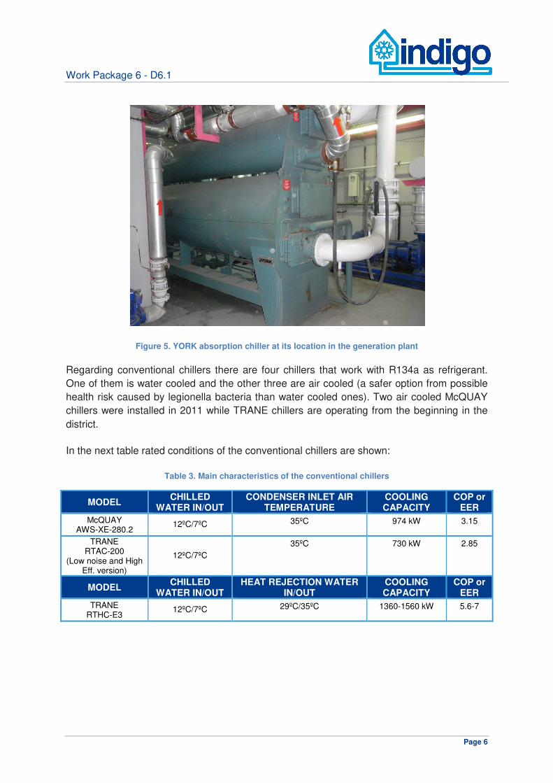
Figure 5. YORK absorption chiller at its location in the generation plant
Regarding conventional chillers there are four chillers that work with R134a as refrigerant.
One of them is water cooled and the other three are air cooled (a safer option from possible
health risk caused by legionella bacteria than water cooled ones). Two air cooled McQUAY
chillers were installed in 2011 while TRANE chillers are operating from the beginning in the
district.
In the next table rated conditions of the conventional chillers are shown:
Table 3. Main characteristics of the conventional chillers
MODEL CHILLED
WATER IN/OUT CONDENSER INLET AIR
TEMPERATURE COOLING CAPACITY
COP or EER
McQUAY AWS-XE-280.2
12ºC/7ºC 35ºC 974 kW 3.15
TRANE RTAC-200
(Low noise and High Eff. version)
12ºC/7ºC
35ºC 730 kW 2.85
MODEL CHILLED
WATER IN/OUT HEAT REJECTION WATER
IN/OUT COOLING CAPACITY
COP or EER
TRANE RTHC-E3
12ºC/7ºC 29ºC/35ºC 1360-1560 kW 5.6-7

Work Package 6 - D6.1
Page 7
Figure 6. McQUAY conventional chiller at its location in the roof of the generation plant
Figure 7. TRANE air cooled conventional chiller at its location in the roof of the generation plant

Work Package 6 - D6.1
Page 8
Figure 8. TRANE water cooled conventional chiller at its location in the generation plant
The cold energy produced by each chiller is recorded by an energy meter installed in the
corresponding cold water circuit. In the same way the total cold energy produced by the plant
is also recorded in another energy meter connected to the main pipes of the district cooling
network.
2.1.2.2. Cold water storage
Outside the generation plant building there is a buffer tank for cold water that is connected
between the return and supply manifolds as it can be seen in the Figure 3. The buffer tank
has a volume of 26 m3 (diameter 2.5 m, height 5.38 m) and it is employed for absorbing the
flow variations between the flow from chillers and the flow sent to the buildings.

Work Package 6 - D6.1
Page 9
Figure 9. Buffer tank sitting outside the generation plant building
2.1.3. Distribution
The cold water produced in the generation plant is distributed to the consumers (buildings)
through a pumping station and a piping layout that can be seen in Figures 2 and 3. From the
pumping station installed inside the generation plant, the pipes extends to the different
buildings through the underground galleries available to interconnect buildings. The length of
the piping is about 2 km (supply + return) split in two branches. The DC network sends cold
water to nine buildings where substations are installed. The total number of substation is
eleven because in two of the buildings there are two substations.

Work Package 6 - D6.1
Page 10
Figure 10. One of the underground galleries of the Hospital with the pipes of DC and DH installed in the ceiling (upper left corner)
2.1.3.1. Distribution layout
Next figure represents the distribution layout of the installation where the two branches and the
different substations can be distinguished
Figure 11. Layout of the distribution of the DC

Work Package 6 - D6.1
Page 11
2.1.3.2. Piping
All the pipes employed in the grid are made of black steel DIN 2448 and DIN 2440. The size
of the pipes for distribution ranges from DN 14" (main supply and return pipes) to DN 6"
(pipes connecting the last building in the longest branch).
The pipes are insulated with flexible elastomeric nitrile rubber foam (ARMAFLEX type or
similar) with a thermal conductivity of 0.040 [W/m K] at 10°C. The thickness of the insulation
for the piping is in compliance with IT 1.2.4.2.1 Spanish regulation. Taking this regulation into
account and that the pipes are installed indoor (galleries), the thickness is 40mm for all the
distribution piping.
The facility is equipped with all elements necessary for compliance with the Spanish RITE
normative for thermal installations in buildings:
• Shut-off valves to isolate elements of the system
• Filters for pumps and motorized valves protection
• Check valves to prevent unwanted reverse flow
• Hydraulic balancing valves in each substation circuit
2.1.3.3. Pumping station
The pumping station is installed in the Generation plant and consist of four centrifugal pumps
that connects the supply manifold (suction) with the distribution manifold (discharge). These
pumps are connected to a frequency converter giving the possibility of controlling the speed
of the pump (performance curves).
The power of absorption chiller has not been taken into account in the calculation of the
production capacity of the facilities, since its operation is subject to established schedules for
operation of cogeneration engines. So the pumping is dimensioned to deliver 4 MWc
(conventional chillers) but the power installed is more than 5 MWc (including absorption
chillers).

Work Package 6 - D6.1
Page 12
Figure 12. Distribution pumps
2.1.3.4. Substations
The substations are the connecting point between the DC and the consumer. In the case of
this DC there are not conventional heat exchangers separating both sides, instead of that
there are hydraulic separators or decouplers. The separator is a kind of slim tank where two
pipes from distribution side and two pipes from building side are connected.

Work Package 6 - D6.1
Page 13
Figure 13. Hydraulic decoupler in one of the substations
The substation includes one (or more in parallel) regulating valve(s) and one static balancing
valve in the distribution side. Three temperature sensors are available (supply and return in
the building side, return in the distribution side) and connected to the BMS. Apart from that
an energy meter is installed in the building side of the substation. Those meters (Ista
Sensonic II in most of the cases) calculate the energy (cold) consumed by the building. The
consumption of the building is regularly collected via direct readout since remote reading
accessories are not installed nor connected to the BMS.
A typical substation for this installation is represented in the next figure:
Figure 14. Simple diagram of a substation

Work Package 6 - D6.1
Page 14
There are eleven substations and nine buildings (as it can be seen in Figure 11 Makua and
Gurtubay buildings have two substations each) in all the DC network, normally located in the
lowest floor under the buildings (underground) although there are a pair of them located in
the highest floor under the roof (Aztarain and Makua buildings).
The regulating valve is a two way flanged globe valve with a linear actuator from Siemens
(SKC 62) while the static balancing valve is a casting body flanged valve from Tour and
Andersson (STAF).
2.1.4. Consumption
The district is connected to eleven different consumers and the main demand corresponds to
air conditioning (temperature and moisture) of different areas of the different buildings. The
cooling demand is very stochastic since it depends on the number of programmed surgeries
(surgical theatres usage), rooms occupancy level, etc.
At the moment the number of running surgical theatres are twenty two split in different
buildings. In the case of the Areilza (Surgical Block) building, not working at full capacity, it is
possible to put six on service along next year.
Table 4. Number of surgical theatres running in the hospital
BUILDING NUMBER OF SURGICAL THEATRES
Allende 2
Areilza (Surgical Block) 8
Consultas Externas 1
Iturrizar 5
Makua 6
Anyway there are specific medical equipment connected to the DC. The major example is the linear
accelerator placed in San Vicente building.
In the next subsections specific info regarding the consumption side of the DC is given.
2.1.4.1. Building and cooling demands
Most of the buildings that comprehend the hospital are more than one hundred years old
(1908). Although different retrofitting works have taken place along the years in facades and
roofs, buildings maintain their original outward appearance. Two of the buildings (Areilza and

Work Package 6 - D6.1
Page 15
Aztarain) were rebuilt from scratch in the period 2007-2010 with the same spirit but with
modern techniques and materials. A detailed info regarding envelope characteristics for
thermal behaviour determination is only available for these two buildings.
As it was said before the energy consumed by the buildings from the district is collected by
energy meters. Next table shows the energy consumed by each building during the year
2011.
Table 5. Energy consumption (cold water) in the different buildings connected to the DC
BUILDING ENERGY [MWh/year]
( 2011)
Allende 145.206 (3%)
Areilza (Surgical Block) 1333.284 (28.5%)
Aztarain 237.981 (5%)
Consultas Externas 43.737 (0.9%)
Gurtubay 926.484 (20%)
Iturrizar 120.403 (2.6%)
Makua 957.757 (20.5%)
Revilla 829.881 (17.7%)
San Vicente 82.827 (1.8%)
Total 4677.560 (100%)
2.1.4.2. HVAC equipment connected to the substations
The equipment connected to the substation of each building is mainly composed of Air
Handling Units (AHU) and Fan coils. In these equipments the respective cooling coil is the
element connected to the DC through the distribution piping of the building connected to the
substation.
The regulation for HVAC in Hospitals, does not allow recirculation indoor air, therefore all the
recirculation must be made using outdoor air. This means an important energy consumption
in the conditioning of the outdoor air so an energy recovery equipment is commonly installed
in AHU to save as much waste energy as possible.

Work Package 6 - D6.1
Page 16
Figure 15. Screenshot from the BMS interface where one of the AHUs (with energy recovery) installed in Areilza (Surgical Block) building can be seen in detail
Figure 16. Screenshot from the BMS interface where two Fan coils installed in Areilza (Surgical Block) building can be seen in detail
Next table shows the installed number of AHU and Fan coils connected to the DC in the
different buildings:
Work Package 6 - D6.1
Page 17
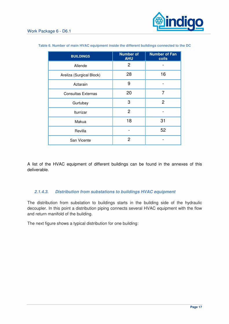
Table 6. Number of main HVAC equipment inside the different buildings connected to the DC
BUILDINGS Number of
AHU Number of Fan
coils
Allende 2 -
Areilza (Surgical Block) 28 16
Aztarain 9 -
Consultas Externas 20 7
Gurtubay 3 2
Iturrizar 2 -
Makua 18 31
Revilla - 52
San Vicente 2 -
A list of the HVAC equipment of different buildings can be found in the annexes of this
deliverable.
2.1.4.3. Distribution from substations to buildings HVAC equipment
The distribution from substation to buildings starts in the building side of the hydraulic
decoupler. In this point a distribution piping connects several HVAC equipment with the flow
and return manifold of the building.
The next figure shows a typical distribution for one building:

Work Package 6 - D6.1
Page 18
Figure 17. Screenshot from the BMS interface where the distribution to the HVAC equipment can be seen in the Areilza (Surgical Block) building substation
All the pipes employed are made of black steel DIN 2448 and DIN 2440. The pipes are
insulated with flexible elastomeric nitrile rubber foam (ARMAFLEX type or similar) with a
thermal conductivity of 0.040 [W/m K] at 10°C. The thickness of the insulation for the piping
is in compliance with IT 1.2.4.2.1 Spanish regulation. The pumping is commonly done by twin
pumps (alternative operation) with speed control for adapting the flow to the demand. The
number of twin pumps depends on the number of main branches in the building (in Figure 17
two main branches can be identified).
2.1.5. Operation and control of the installation
Related to the generation system strategy, the trigeneration plant schedule is worked out
according to the electricity price. The internal combustion engines are operated daily (manual
or automatic start) during high electricity prices, thus prioritizing electricity generation.
During this period heat from cogeneration is stored
(hot water) and used for hospital demand and for cooling generation (absorption chillers) and
the difference with respect to the cooling demand is covered by a pre-established electrical
chillers start sequence management. For the rest of the time (no electric energy generation)
another electrical chillers start sequence and cold water storage (buffer for internal chillers
management) is automated.

Work Package 6 - D6.1
Page 19
The operation of the DC system is based on a management control that interacts just with
the controllers of each chiller. It controls distribution pumps (differential pressure control
between impulse and return), but not the temperature set point at substations.
2.1.5.1. System structure and Monitoring&Control
In terms of Monitoring and Control, the Basurto Hospital DC network is divided, as explained,
in Generation (and water distribution) and Consumption (Buildings).
The system commanding these two sides are different.
The Monitoring and Control installed in the generation side (comprehending the gas engines,
chillers, etc.) is made of scada modules programmed by Veolia and Genelek (local company
with expertise in automation), following this architecture:
Generation side
Figure 18. Genelek customized PLC topology
Consumption side
In the next figure the installed Desigo Insight BMS from Siemens is represented

Work Package 6 - D6.1
Page 20
Figure 19. SIEMENS Desigo Insight topology
2.1.5.2. Operation philosophy
Generation
Absorption chillers and cogeneration engines
There is a Schedule already programmed for the start/stop of the cogeneration engines,
depending on electricity prices, there are two different general schedules for the
cogeneration engines, winter time and summer time:
In winter time, one engine normally works from 7:00 to 24:00 and the other can vary, working
in between 12:00 to 17:00. This is important because of feeding the absorption chillers with
hot water coming from the cogeneration engines.
The general heat control PLC at generation calculates the difference between the flow of hot
water produced by the cogeneration engines and the flow of hot water consumed by the
Hospital (comfort heat and sanitary water). The difference corresponds to the flow available
to be accumulated in the storage tanks and / or consumed by the absorption machines . The
value of this flow available will be sent to the general cold control PLC and it will be used to
decide whether or not start absorption machines and to regulate them .
As a matter of fact, absorption chillers have always priority at time of producing cold water
for the DC.
Anyway, in winter season, the York absorption chiller is out of run due to low cold demand.
Work Package 6 - D6.1
Page 21
Normally, in winter time, when the cogeneration engines start at 7:00 they feed the 6 x 25 m3
storage tanks with the hot water generated, absorption chillers don’t run and the hot water is
used for heating.
At 12:00, if cold is needed, the BROAD absorption chiller starts working. If cold water is
needed before, a Mc Quay electric chiller will help.
In summer season (between May and November) the two absorption chillers will work .
Normally, as there is not such a need for hot water in the hospital during summer time, the
BROAD chiller starts working at the same time that cogeneration engines, using directly part
of the hot water generated. YORK chiller will follow it and some hot water will still be storage
in the tanks.
Chillers cascade control
Depending on cold demand from the hospital, the regulation will be starting machines in
cascade so that the driving flow temperature never rises the established maximum
temperature the (ideally 12ºC for maximum performance).
The logic control is:
Cold water theoretically is always sent to the hospital at 7 ºC and returns at 10/12 ºC, so the
only variable is the flow that is sent to the hospital. When cold demand in the buildings rises,
the regulation will increase the supply flow and inversely, when the demand goes down, it is
a lower flow distribution.
The six chillers work always between 7-12ºC, it is understood that at all times the number of
running chillers must be such that the sum of the flows from the active chillers is greater than
or equal to the flow rate is sent to the hospital.
Again, we can differentiate between two different ways of working:
Winter stage (December-April)
As said before, Cogeneration engines are key in cold water production through the
absorption chillers, so when they start, they fill up the hot storage tanks.
In the meanwhile, in the first hours of the morning, if cold water is needed and absorption
chillers are not ready, the Mc Quay electric chillers will supply water to the network.
At 12:00, the BROAD absorption chiller will start, stopping the first Mc Quay that will run
again if needed. After, the second electric McQuay will start and finally, the air TRANE RTAC
air condensed.
Neither TRANE RTHC water condensed nor YORK absorber chiller water condensed are
programmed to work in winter stage.
Summer stage (May-November)

Work Package 6 - D6.1
Page 22
In summer stage, as there is no need of much hot water for the hospital (no heating needed)
hot water provided by cogenerators can be fully used for the absorption chillers.
So, at 7:00 the BROAD will start, followed by the YORK, followed by the two Mc Quay (2 x
1000 kW) and if more cold is needed the TRANE RTHC (1.400 kW) stopping then one Mc
Quay.
Should more cold water is needed, this Mc Quay will start again, being the last one in use the
TRANE RTAC due to be the oldest machine in place with the worse COP.
Distribution (pumping)
The operation of the pumping station that sends chilled water to the buildings is controlled by
a pressure setpoint between the supply and distribution manifold (see Figure 3). A differential
pressure transducer and a PI control loop drives the pumps (speed) to assure the setpoint.
Pumps operate in a consecutive way, that is, the second pump does not start until the first
pump is at maximum speed and so on.
The differential pressure setpoint is not constant but dependent on the ambient temperature
according to the next figure:
Figure 20. Differential pressure setpoint relation with ambient temperature
Consumption (substations)
According to the Figure 14 the elements that participate in the control of the substations are:

Work Package 6 - D6.1
Page 23
• One (or more in parallel) two-way motorized valve(s).
For example in the case of Surgical Block building there are five valves arranged in
parallel due to the large flow rate. These five valves are divided in two groups: one
group of two valves and another one of three valves. Regulation starts opening
progressively the first group (both valves together at the same time) until valves are
completely open. If more flow is needed, then the second group starts opening (the
three valves at the same time). In the case that a flow reduction is needed, the
procedure is exactly the other way around.
• One temperature sensor in the building supply
• One temperature sensor in the distribution return
The control of the regulating valve(s) need to assure that the distribution side return
temperature is always above a setpoint that is commonly fixed in 10ºC (is not possible to
reach the ideal return temperature of 12ºC in most of the substations).
2.1.6. Available monitoring data
2.1.6.1. Generation
Regarding the generation plant, available data correspond to every minute measurements of
the next magnitudes since August 2011:
• Cold water produced in each chiller (energy meter)
• Hot water employed for feeding each absorption chiller (energy meter)
• Electric consumption in each chiller
• Gas consumption of cogeneration engines
• Supply and return temperature of the cold water circuit produced by each chiller
• Supply and return temperature of the driving hot water circuit of each absorption
chiller
• Supply and return temperature of heat rejection water circuits (cooling towers)
• Water temperature in the supply and return manifolds
• Water pressure in supply and return of cooling ring (DC)
• Water temperatures at the top and the bottom of the buffer tank
• Outdoor temperature (surroundings of the generation plant building)

Work Package 6 - D6.1
Page 24
2.1.6.2. Distribution
Regarding the cold water distribution, the monitoring data can be obtained only at substation
level through the Siemens Desigo Insight BMS. This system allows reading next magnitudes
(for each substation of the DC) according to the Figure 14:
• Distribution side: Return water temperature
• Distribution side: Position/s of the regulating valve/s (% opening)
• Building side: Supply and return water temperature
Currently the BMS has not included the features for automatic record of measurements
(Historical data) and it is only possible to create small record files with limited capabilities
called "Trends". Each Trend can store up to nine measurements with an user defined sample
time and a fixed maximum file size. These Trends can be defined and download only in the
PC installed in the Areilza building (Surgical Block).
It is planned to upgrade the collecting of consumption data installing some new meters at
each substation. These meters shall be bus-connected in order to have monitor iced
readings. All this info will be included in the first version of the Deliverable D6.3.
2.1.6.3. Consumption
As in the case of the Distribution, the data come from the Siemens Desigo Insight BMS.
These data are limited to only one building, Areilza building (Surgical Block) where the
different components of the installation inside the building are monitored (see Figures 15, 16
and 17).
As it is mentioned in the above section, Historical data are not available but some trends
have been created for different elements of the installation in order to help the Maintenance
crew locating source of performance problems of the building installations.

Work Package 6 - D6.1
Page 25
2.2. LA MARINA SITE
2.2.1. General description
La Marina DH&C network is placed in L'Hospitalet de Llobregat a city next to Barcelona,
Spain. This installation is going to be part of a bigger deployment with the aim of servicing
Barcelona urban area. Ecoenergies Barcelona (VEOLIA) is the company name that was
created for the construction, management, operation and exploitation of the complete
installation.
The installation is running since 2013 and currently the generation plant of the installation is
composed of three water condensed electric chillers and three gas boilers. The plant is
placed inside Fira 2000, the new trade fair of Barcelona, and gives service to different
costumers in the area: A Hotel, a shopping center, two office buildings and two pavilions of
the trade fair. The distribution has a total length of 12 km (supply and return) and is divided in
three branches.
The DC temperature level is 5ºC in flow and 14ºC in return while the DH temperature is 90ºC
in flow and 60ºC in return.
In the next picture the main layout of La Marina DC network can be seen. The dark blue
arrow points to the generation plant while the white arrows point to the consumers. The three
main branches of the network can be identified (solid blue lines).
Figure 21. La Marina DC main layout
After this brief introduction the document will focus in the DC part of the installation.

Work Package 6 - D6.1
Page 26
2.2.2. Generation plant
The generation plant is located at underground level in Barcelona trade fair and there,
chillers, pumping station and control can be found (Figure 21).
2.2.2.1. Chilled water production
The Figure 22 shows a simple diagram of the main elements inside the generation plant. As
it can be seen the chillers are connected in parallel between the supply and return manifolds.
Figure 22. Generation plant simplified layout
The chillers work with R-134a as refrigerant and the main characteristics of the two different
chiller models are shown in the next table:
Table 7. Main characteristics of the chillers
MODEL CHILLED WATER
IN/OUT HEAT REJECTION WATER
IN/OUT COOLING CAPACITY
COP or EER
2 x McQUAY
WDC126MB
194 l/s
14ºC/5ºC
410 l/s
30/35ºC
7.33 MWt 5.51
McQUAY WSC087MA
53 l/s
14ºC/5ºC
113 l/s
30/35ºC
2 MWt 5.45
The cooling water circuit of each chiller is driven by a pump with a speed control (frequency
converter) assuring a constant temperature and variable flow production.
The installation has five cooling towers (with variable speed fan) connected in parallel for
heat rejection from chillers. Each rejection circuit is connected to a small supply and return

Work Package 6 - D6.1
Page 27
manifold where cooling towers are connected. These chiller rejection circuits have a variable
speed pump.
2.2.2.2. Cold water storage
The installation does not include any cold water storage or buffer tank.
2.2.3. Distribution
2.2.3.1. Distribution layout
The next figure represents the distribution layout of the installation where the three branches
and the different consumers can be distinguished:
Figure 23. Distribution simplified layout
The Fira branch is currently the less demanding part of the installation due to its direct
relation with the scheduled expositions. The SERTRAM office building and the Clients part of
the IBERDROLA building has been connected to the network on 2016.

Work Package 6 - D6.1
Page 28
2.2.3.2. Piping
Pipes employed in the generation plant are made of ,on site insulated, black steel DIN 2453
pipes while for the pipes out of the plant (buried) pre-insulated pipes of the same material
(black steel) are employed. The size of the pipes for distribution ranges from DN600/DN400
in the outlet of the distribution manifolds to DN50 in certain substations.
2.2.3.3. Pumping station
The pumping station is installed in the generation plant and consist of three groups of pumps
(one per branch) as it can be seen in Figure 22. These pumps are connected to frequency
converters so their speed (performance) is controlled. As it can be seen an small pipe
connects supply and return manifolds. In this pipe a flow detector is installed with the aim of
balancing production pumping (chillers) with distribution pumping. Depending on the flow
fixed in the distribution (defined for assuring contracted service, 5.5 ºC distribution side
supply, to the last consumer) the flow in the chillers is defined looking for a no flow condition
in the manifolds connecting pipe.
2.2.3.4. Substations
The substations are the interface between the DC and the consumer (building). In this
installation a flat plate heat exchanger is installed in each substation for assuring the thermal
energy transfer between production side and demand side. Next figure shows a typical
substation diagram with the main components.
Figure 24. Diagram of a substation
Main elements of the substation are:

Work Package 6 - D6.1
Page 29
Distribution side
• Differential pressure valve
• Regulating valve (temperature control)
• Supply and return water temperature
• Energy meter
Building side
• Supply and return water temperature
• Flow switch
All the components that conform the substation belongs to the client (starting from the pipes
that connect the heat exchanger with the distribution branch ). For that reason the
components are not exactly the same for all the clients. The substations that were built at the
same time as the network was, employed the same components but clients that were
connected afterwards usually employed equivalent components that performed the same
function but that belongs to different manufacturers. The only condition fixed by the operator
is to employ components certified for DH&C installations.
2.2.4. Consumption
The district is connected to six different consumers and the main demand corresponds to air
conditioning.
2.2.4.1. Cooling demands
Next table shows the power installed and the energy consumed by each building along three
consecutive years (2013, 2014 and 2015) and an estimation for 2016. The energy consumed
data come from the energy meters installed in each substation.

Work Package 6 - D6.1
Page 30
Table 8. Installed power and annual energy consumed by clients connected to the DC
BUILDING
POWER INSTALLED
[kW]
ENERGY CONSUMED [MWh/year]
(2013)
ENERGY CONSUMED [MWh/year]
(2014)
ENERGY CONSUMED [MWh/year]
(2015)
ENERGY CONSUMED [MWh/year]
(2016)*
Fira Pavilions 5&7 8350 161.3 (3.5%) 581.5 (8.1%) 304.32 (5.4%) 407.01 (5%)
Gran Via 2 Shopping Centre
3000 3973 (87%) 5204.4
(72.6%)
4152.6
(73.7%)
4878.95
(60.3%)
Hotel SB 850 61
(1.3%)
858.1 (12%) 923.6 (16.4%) 891.65 (11%)
Sertram office building
400 0 0 0 1076.85
(13.3%)
Iberdrola office building, ZC
310 361.4 (8.2%) 523.9 (7.3%) 249.83 (4.5%) 395.57 (5%)
Iberdrola office building, Clients
262.5 0 0 0 435.29 (5.4%)
Total 13172.5 4556.7 7167.9 5630.35 8085.32
* Estimated
2.2.4.2. HVAC equipment connected to the substations
The equipment connected to the heat exchanger in the buildings is composed of AHU and
fan coils in all the cases.
2.2.4.3. Distribution from substations to buildings HVAC equipment
The distribution from substation to buildings starts in the building side of the heat exchanger.
In this point a distribution piping connects several HVAC equipment with the flow and return
manifold of the building.
The regulation of all terminal equipment inside the building is performed with variable flow
(constant temperture) employing two-way control valves and thus, avoiding any water
mixture circuit with the return.
2.2.5. Operation and control of the installation
2.2.5.1. System structure and Monitoring&Control
Here is the architectural scheme of the system structure:

Work Package 6 - D6.1
Page 31
Figure 25. Topology of the system
2.2.5.2. Operation philosophy
Generation
The operation of the DC system is based on a management control that interacts just with
the controllers of each chiller. The pumps associated to each chiller are controlled to assure
constant temperature in the outlet (5ºC) according to the demand. The flow through the
chiller is determined to fit the flow in the distribution as it has been explained before.
Distribution (pumping)
The operation of the pumping station that sends chilled water to the buildings is controlled by
a setpoint of pressure between the supply and distribution manifold . A differential pressure
transducer and a PI control loop drives the pumps (speed) to assure the setpoint. The
differential pressure setpoint is variable and is fixed by the operator (manually) assuring
supply in terms of the contract (5.5ºC on the distribution side supply) to the farthest client of
the network.
Each group of pumps (one group for each branch) operate in a consecutive way, that is, the
second pump does not start until the first pump is at maximum speed.
Consumption (substations)
In each substation it is installed a control system comprising:

Work Package 6 - D6.1
Page 32
• One motorized two-way valve for flow controlling
• One temperature sensor in the supply to the building
• One temperature sensor in the return from the building
• One temperature sensor in the supply from the distribution
• One temperature sensor in the return to the distribution
• An energy meter in the distribution side
There are two different possibilities of control in the substation and the selection criteria
depends on the temperature difference that the building (client) works with during normal
operation. Commonly, already existing buildings that are connected to the network work with
a low temperature difference while new buildings, with newer installations, work with higher
temperature difference. For the first case (low difference) the type of control has as setpoint
the flow temperature to the building (depends on the client and the season) while for the
second one the control is based on the design return temperature to the distribution (14ºC).
The setpoint for both cases is remotely fixed by the operator of the DC with the permission of
the client.
2.2.6. Available monitoring data
2.2.6.1. Generation
Regarding cold water production, the data that is obtained from the installation is the
following one:
• Energy meters (kWh cold water) in every chiller
• Electric consumption in every chiller, every pump, every cooling tower
• Water temperature sensors in supply and return of all chillers
• Water temperature sensors in supply and return of cooling towers circuit
• Water temperature sensors in distribution manifold and return manifold
• Water pressure sensors in supply and return manifolds
• Environmental temperature sensors (surroundings of the generation plant)
Historical data is available since 2013 for these magnitudes:
• Cold water produced in each chiller (kWh and m3)
• Electric consumption in each chiller (kWh)
• Temperatures:
o Cold water supply from each chiller (ºC)
o Cold water return to each chiller (ºC)
o Cold water supply from each cooling tower (ºC)
o Cold water return to each cooling tower (ºC)

Work Package 6 - D6.1
Page 33
o Cold water supply in main manifold
o Cold water to general return manifold
• Outside plant temperature.
Readings can be obtained every second if needed. These data is collected in a .csv file that
is automatically generated by the system.
2.2.6.2. Distribution
Regarding cold water distribution, the data obtained from the system is:
• Energy sent to the substation (kWh cold water) for a period
• Volume of cold water passed through the substation for a period
• Instantaneous power sent to the substation
• Instantaneous water flow in the distribution side
• Supply temperature from the heat exchanger
• Return temperature from the heat exchanger
• % opening of the motorized two-way control valve
Historical data is available since 2013. Readings can be obtained every second if needed.
These data is collected in a .csv file that is automatically generated by the system.
2.2.6.3. Consumption
Regarding cold water distribution, the data obtained from the system is :
• Supply temperature to the building
• Return temperature from the building
Historical data is available since 2013. Readings can be obtained every second if needed.
These data is collected in a .csv file that is automatically generated by the system.

Work Package 6 - D6.1
Page 34
2.3. ZONA FRANCA SITE
2.3.1. General description
La Zona Franca DH&C network is placed in Barcelona, close to the harbour, an strategical
point regarding logistics. As in the case of La Marina, Zona Franca, is going to be part of a
bigger installation with the aim of servicing Barcelona urban area. Ecoenergies Barcelona
(VEOLIA) is the company name that was created for the construction, management,
operation and exploitation of the complete installation.
In the next picture it can be seen a layout of the big DHC project of Barcelona
Figure 26. Layout of the Barcelona DH&C project
La Marina installation is identified in the picture with number 2 while Zona Franca installation
is identified with number 1. The installation identified with the number 3 represents a future
installation that will act as a free cooling source coming from the phase change (gasification)
of LNG discharged in the harbour by big LNG carriers.
The installation is running since 2013 and currently the generation plant of the is composed
of two water condensed electric chillers and one boiler. The plant is placed close to the
Barcelona Port and gives service to only two consumers at the moment, both related to food
industry (storage and process).
The DC is splitted in two different networks for two different temperature levels: -10ºC flow (-
4ºC in return) and 5ºC flow (14ºC return). The DC for 5ºC cooling supply is currently a quite

Work Package 6 - D6.1
Page 35
small installation and only serves to one of the already mentioned costumers with a reduced
power (50kWt). Due to that, only the DC for -10ºC cooling supply will be consider in this
project.
The distribution network has a total length of around 1.4 km (supply and return) that belongs
to the first part of the main branch of the projected installation in Zona Franca.
In the next picture the main layout of the Zona Franca DC network can be seen. The dark
blue arrow points to the generation plant while the white arrows point to the consumers. As it
can be seen the branch continues to the right but there is no flow due to the lack of clients at
the moment.
Figure 27. Zona Franca main layout
2.3.2. Generation plant
The generation plant is located in a specific building constructed as the main building of the
big DH&C project of Barcelona. There, chillers, pumping station and control can be found
(apart from DH related equipment and other installations).

Work Package 6 - D6.1
Page 36
2.3.2.1. Chilled water production
Figure 28 shows a reduced diagram of the main elements inside the generation plant. The
cold water production is done with the same compressors independently of the temperature
level. This is done thanks to a little bit complex installation composed of three different
temperature level manifolds, condensers, vessels, an economizer and two separators (one
per temperature level). Each separator is connected to a flat plate heat exchanger where the
supply and return manifolds of each temperature level DC are connected. For simplicity, in
the installation layout the cold production is limited to the already mentioned heat exchanger.
Figure 28. Generation plant reduced layout
The cooling liquid that flows in the installation is a water-propylenglycol mixture with a 30% to 40% by mass ratio of propylenglycol. The chillers work with Ammonia (R-717) as refrigerant and the main characteristics of the
two different chiller models are shown in the next table:
Table 9. Main characteristics of the chillers
MODEL EVAPORATION TEMPERATURE
CONDENSATION TEMPERATURE
COOLING CAPACITY
COP
MYCON NV250 VMDD-ME
-15ºC
35ºC
1.197 MW
3.7
MYCON N170 JL-L
-15ºC
35ºC
0.509 MW
3.86
The plant works in a variable flow - constant temperature configuration scheme as the rest of the sites. The main equipment of the installation is:

Work Package 6 - D6.1
Page 37
• Two ammonia compressors
• Two evaporative cooling towers
• Two liquid-gas separators
• Two flat plate heat exchangers
• One Economizer
Figure 29. MYCON NV250 ammonia compressor
Figure 30. Flat plate heat exchanger for ammonia and water-propylenglycol mixture
2.3.2.2. Cold water storage
There is not a cold water storage neither in the generation plant, nor in the distribution
network.

Work Package 6 - D6.1
Page 38
2.3.3. Distribution
2.3.3.1. Distribution layout
In the following figure it is shown the distribution lay out for Zona Franca DC.
Figure 31. Distribution simplified layout
At the moment there are only two clients: Acciona with a cold demand only for storing food (-
7ºC) and APA with a cold demand for storing (-7ºC) and feeding of equipment for food
processing (-5ºC).
2.3.3.2. Piping
All the pipes inside the generation plant employed for the -10ºC supply temperature are
black steel DIN 2440 of different nominal diameters and adequate insulation thickness to
avoid energy losses and condensation. For the distribution part pre-insulated pipes of the
same material are employed.
Installation is completed with a series of elements such as shut-off valves (butterfly , ball ..),
balancing valves, check valves, control valves, two and three-way valves, safety valves,
filling and emptying valves, air vents, Y shaped filters, pressure gauges, thermometers, flow
detectors, etc.

Work Package 6 - D6.1
Page 39
2.3.3.3. Pumping station
The pumping station is installed in the generation plant and consist of two pumps for
supplying consumers and two pumps for extracting the cold from the heat exchanger as it
can be seen in Figure 28. All these pumps are connected to frequency converters so their
speed (performance) is controlled. In the same figure pipe connects supply and return
manifolds and in this pipe a flow detector is installed with the aim of balancing production
pumping (heat exchanger) with distribution pumping. Depending on the flow fixed in the
distribution (defined for assuring contracted service, -10 ºC distribution side supply, to the
last consumer) the flow in the heat exchanger (water-propylenglycol mixture side) is defined
looking for a no flow condition in the pipe connecting manifolds.
2.3.3.4. Substations
Next figure shows a typical substation:
Figure 32. Diagram of a typical substation
Main elements of the substation are:
Distribution side:
• Differential pressure valve
• Regulating valve (temperature control)
• Supply and return water temperature
• Energy meter
Client side:
Work Package 6 - D6.1
Page 40
• Supply and return water temperature
• Flow switch
All the components that conform the substation belongs to the client (starting from the pipes
that connect the heat exchanger with the distribution branch ). For that reason the
components are not exactly the same for all the clients. The substations that were built at the
same time as the network was, employed the same components but clients that were
connected afterwards usually employed equivalent components that performed the same
function but that belongs to different manufacturers. The only condition fixed by the operator
is to employ components certified for DH&C installations.
2.3.4. Consumption
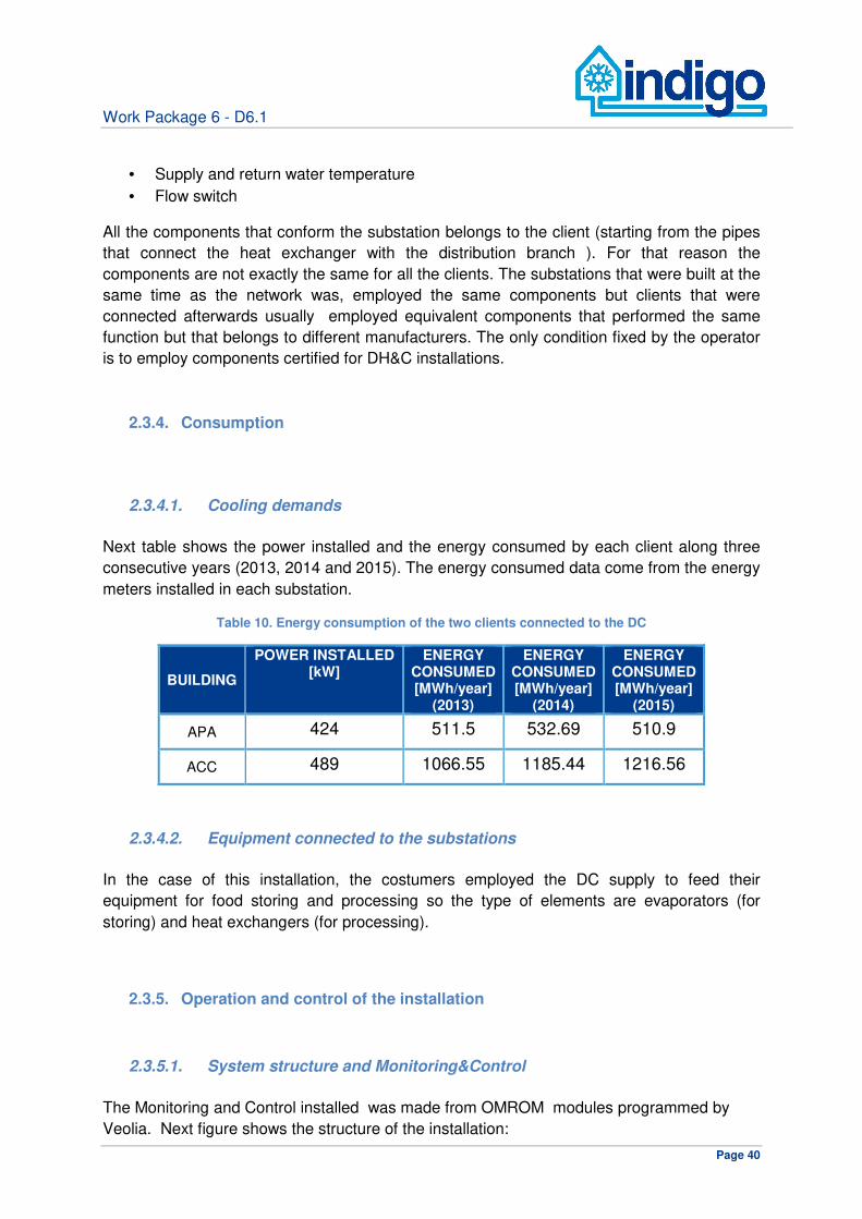
2.3.4.1. Cooling demands
Next table shows the power installed and the energy consumed by each client along three
consecutive years (2013, 2014 and 2015). The energy consumed data come from the energy
meters installed in each substation.
Table 10. Energy consumption of the two clients connected to the DC
BUILDING
POWER INSTALLED [kW]
ENERGY CONSUMED [MWh/year]
(2013)
ENERGY CONSUMED [MWh/year]
(2014)
ENERGY CONSUMED [MWh/year]
(2015)
APA 424 511.5 532.69 510.9
ACC 489 1066.55 1185.44 1216.56
2.3.4.2. Equipment connected to the substations
In the case of this installation, the costumers employed the DC supply to feed their
equipment for food storing and processing so the type of elements are evaporators (for
storing) and heat exchangers (for processing).
2.3.5. Operation and control of the installation
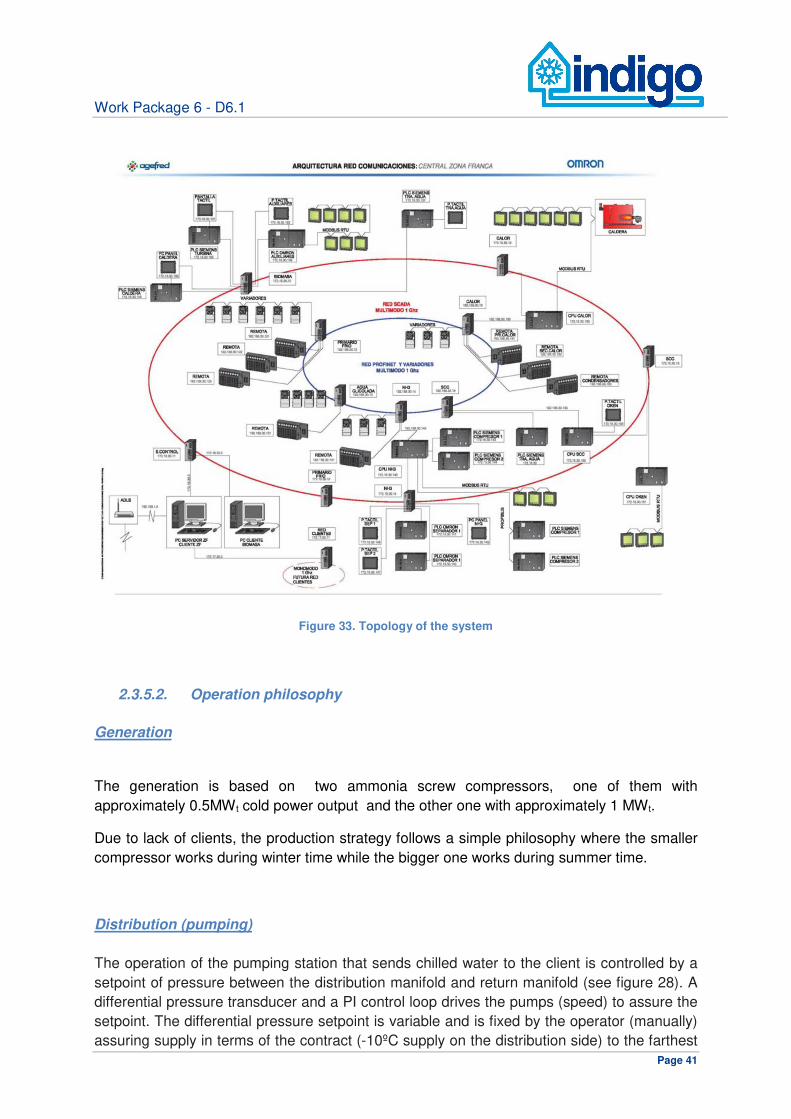
2.3.5.1. System structure and Monitoring&Control
The Monitoring and Control installed was made from OMROM modules programmed by
Veolia. Next figure shows the structure of the installation:
Work Package 6 - D6.1
Page 41
Figure 33. Topology of the system
2.3.5.2. Operation philosophy
Generation
The generation is based on two ammonia screw compressors, one of them with
approximately 0.5MWt cold power output and the other one with approximately 1 MWt.
Due to lack of clients, the production strategy follows a simple philosophy where the smaller
compressor works during winter time while the bigger one works during summer time.
Distribution (pumping)
The operation of the pumping station that sends chilled water to the client is controlled by a
setpoint of pressure between the distribution manifold and return manifold (see figure 28). A
differential pressure transducer and a PI control loop drives the pumps (speed) to assure the
setpoint. The differential pressure setpoint is variable and is fixed by the operator (manually)
assuring supply in terms of the contract (-10ºC supply on the distribution side) to the farthest

Work Package 6 - D6.1
Page 42
client of the network. Each pump operate in a consecutive way, that is, the second pump
does not start until the first pump is at maximum speed and so on.
Consumption (substations)
In each substation the installed control system comprises:
• One motorized two-way valve for flow controlling
• One temperature sensor in the supply to the client
• One temperature sensor in the return from the client
• One temperature sensor in the supply from the distribution
• One temperature sensor in the return to the distribution
• An energy meter in the distribution side
The regulating valve in each substation is connected to a controller that assures that the
temperature of the water in the supply to the clients (cold water employed in their installation)
fits the setpoint temperature (-5ºC for storing food and -7ºC for processing).
2.3.6. Available monitoring data
2.3.6.1. Generation
The data obtained from the installations is the following one:
• Energy meter (kWh cold water) in the ammonia-water propylenglycol mixture heat
exchanger
• Electric consumption in every chiller, every pump and every cooling tower
• Water temperature sensors in supply and return of all chilled water production
• Water temperature sensors in supply and return of cooling towers circuit
• Water temperature sensors in supply and return of cooling ring (DC)
• Water pressure sensors in supply and return of cooling ring (DC)
• Outdoor temperature sensor (outside of Generation plant)
Historical data since 2013 are stored:
• Cold water produced in each chiller (kWh and m3)
• Electric consumption in each chiller (kWh)
• Temperatures:
o Cold water supply from each chiller (ºC)
o Cold water return to each chiller (ºC)
o Cold water supply from each cooling tower (ºC)

Work Package 6 - D6.1
Page 43
o Cold water return to each cooling tower (ºC)
o Cold water supply in main manifold
o Cold water to general return manifold
o Outside plant temperature
Readings can be obtained every second if needed. These data is collected in a .csv file that
is automatically generated by the system.
2.3.6.2. Distribution
Regarding cold water distribution, the data that can be obtained from the system is :
• Supply temperature to the substation (heat exchanger)
• Return temperature from the substation
• Instantaneous thermal power send to the substation
• Energy consumed by the client in a certain period
• Volume of cold water sent to the client in a certain period
• % opening control valve
Historical data is available since 2013. Readings can be obtained every second if needed.
These data is collected in a .csv file that is automatically generated by the system.
2.3.6.3. Consumption
Regarding cold water distribution, the data obtained from the system is :
• Supply temperature to the building
• Return temperature from the building
Historical data are available since 2013. Readings can be obtained every second if needed.
These data is collected in a .csv file that is automatically generated by the system.

Work Package 6 - D6.1
Page 44
3. VALIDATION SCENARIOS AND ASSOCIATED TEST PLAN
3.1. INTRODUCTION
INDIGO involves the development of highly efficient and intelligent DC systems based on the
development of an innovative and optimized DC system Management Strategy.
One of the main characteristics of this strategy is the predictive management: The INDIGO
DC system manager will consider predicted values for the consumers' demand, the
meteorological conditions, and the price of energy to establish the DC system components
appropriated set-points for an optimized operation (energy efficiency maximization with
economic cost minimization).
The developed management system will also address other challenges such as:
• Integration of Renewable Energy Sources (RES), which involves additional difficulty
since they are non-manageable energies
• Dealing with different types of cooling sources (different dynamic behavior) at the
same time
• Combining the cooling capacity coming from the generation, storage, and even
distribution (piping storage capacity) and buildings (thermal mass management) in an
optimized way.
• Dealing with different types of thermal storage systems: sensible heat (cold water
storage) and latent heat (ice storage)
These characteristics must be checked through some validation scenarios, which are based
on the test sites previously described.
Nevertheless, in some cases, the tests sites does not contribute to the proper analysis of
INDIGO characteristics, since some of the components required are not currently present in
the test site, such as RES (the case for all of the sites) or storage systems. Therefore, some
of the validation scenarios proposed will be tested virtually.
3.2. VALIDATION SCENARIOS
The first validation scenario, scenario 0, is the most basic one and is entirely based on the sites as they are today. The rest of scenarios, based on scenario 0, include components that currently do not belong to the site, but which contribute to the proper validation of the INDIGO toolkit.
Therefore, two type of scenarios will be proposed apart from the reference one (scenario 0):

Work Package 6 - D6.1
Page 45
• Experimental validation scenario (Basurto Site): INDIGO solution will be physically implemented and ran
• Virtual (or laboratory) validation scenario (La Marina, Zona Franca and Basurto Site): INDIGO solution will be virtually deployed
Next tables define the validation scenarios proposed for the project:

Work Package 6 - D6.1
Page 46
VS-0
Ob
jecti
ves
In this basic validation scenario, the evaluation of the Sites with the INDIGO predictive management strategy will be performed. The current generation, distribution and consumption system will be only considered, as well as the predictive control according to INDIGO.
Energy efficiency maximization with economic cost minimization is the main goal. This goal will be achieved based on the predictive control, considering available information with INDIGO approach:
• Boundary conditions (including weather, demand profile, energy price, etc.)
• Recorded signals (inputs, outputs and relevant data for validation metrics)
In the case of experimental test, it is not possible to get the same boundary conditions and data from site with and without INDIGO, since both control strategies are not possible simultaneously. Therefore, to properly analyze the “before and after” of INDIGO in Basurto site minimizing the uncertainties in the process, two possibilities will be carefully considered:
• Maximizing the period of time in which experimental and historical data are taken with the aim of softening the differences
• Getting an accurate model of Basurto DC system in order to simulate what would have been the energy consumption (or the cost) operating the system with the previous controller (before INDIGO) with the same initial conditions/disturbances (weather, demand due to hospital operations etc)
The reference case for VS0 will be the historical data from its site.
Test
Sit
e
Basurto Site will be tested both virtually and on-site.
Considering the generation and storage systems in Basurto the prior objective will be achieved based on the predictive control and focusing mainly on the electricity consumption reduction during on-peak electricity prize periods:
• Prioritizing the use of absorption chillers
• Prioritizing the use of storage as generation source during on-peak electricity prize periods
• Prioritizing the use of storage as consumer during out-peak electricity prize periods
La Marina Site will be virtually tested.
La Marina Site is composed of electrical chillers but there is no storage systems. Therefore, in this case the prior objective will be achieved based just on the predictive control, considering available information with INDIGO approach.
Zona Franca Site will be left out of this validation scenario due to its constant demand (cold has to be provided to the industries 24h/day, 365 days/year), which does not allow much flexibility to obtain energy savings thanks to the control strategy.
Work Package 6 - D6.1
Page 47
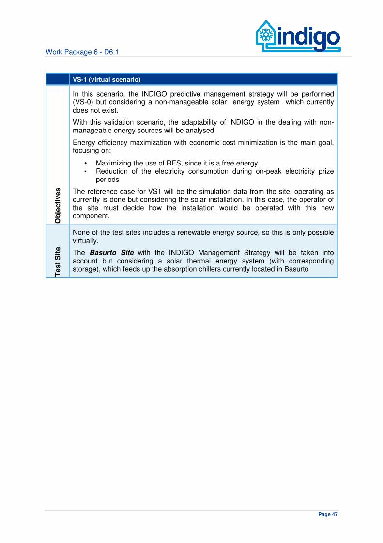
VS-1 (virtual scenario)
Ob
jecti
ves
In this scenario, the INDIGO predictive management strategy will be performed (VS-0) but considering a non-manageable solar energy system which currently does not exist.
With this validation scenario, the adaptability of INDIGO in the dealing with non-manageable energy sources will be analysed
Energy efficiency maximization with economic cost minimization is the main goal, focusing on:
• Maximizing the use of RES, since it is a free energy • Reduction of the electricity consumption during on-peak electricity prize
periods
The reference case for VS1 will be the simulation data from the site, operating as currently is done but considering the solar installation. In this case, the operator of the site must decide how the installation would be operated with this new component.
Test
Sit
e
None of the test sites includes a renewable energy source, so this is only possible virtually.
The Basurto Site with the INDIGO Management Strategy will be taken into account but considering a solar thermal energy system (with corresponding storage), which feeds up the absorption chillers currently located in Basurto

Work Package 6 - D6.1
Page 48
VS-2 (virtual scenario)
Ob
jecti
ves
One of the key systems for INDIGO approach is the use of a storage system, which gives flexibility to obtain energy savings thanks to the control strategy (thanks to MPC and production shifting).
In this validation scenario, the evaluation of the benefits of using storage will be analysed through the versatility of INDIGO in the suitable coupling between generation, storage and demand
Energy efficiency maximization with economic cost minimization is the main goal, focusing on:
• Prioritizing the use of storage as consumer during out-peak electricity prize periods
• Prioritizing the use of storage as generation source during on-peak electricity prize periods
The reference case for VS2 will be the simulation data from the site operating as currently is done but considering an storage system. In this case, the operator of the site must decide how the installation would be operated with this new component.
Test
Sit
e
This virtual scenario will be considered for La Marina Site and Zona Franca Site. The aim in both sites is the same but in this way the flexibility of INDIGO Management Strategy will be analysed at two different temperature levels. In the same way, the INDIGO management with different types of storage will be analyzed, since two different storage will be considered, depending on the water temperature level of the site:
• Cold water storage in La Marina Site • Ice storages in Zona Franca Site
3.3. TEST PLANS DESCRIPTION
Once validation scenarios are defined for the different sites, associated test plans need to be
constructed to define how the validation will be performed in practice.
Next tables describes the different test plans needed for the defined validation scenarios.
The selected naming for the test plan is based on the previously defined naming for the
validation scenarios. As in the case of validation scenarios the test plans are divided in
experimental and virtual (laboratory) level.
The aim of this section is to have an initial description of the test plans according to the
defined validation scenarios. Taking this into account, figures employed for the different
indicators defined as part of the test acceptance criteria of each plan, must be taken as
indicative. In the next phase of the project test plans will be developed and completed
including detailed definition of the indicators (according to international standards) as well as
the figures for targets.

Work Package 6 - D6.1
Page 49
Index of scenarios and corresponding test plans:
• VS0 o EXP_VS0_Basurto_01
o VIRTUAL_VS0_Basurto_01
o VIRTUAL_VS0_Basurto_02
o VIRTUAL_VS0_Basurto_03
o VIRTUAL_VS0_Marina_01
o VIRTUAL_VS0_Marina_02
• VS1 (non-manageable solar energy system) o VIRTUAL_VS1_Basurto_01
• VS2 (using storage) o VIRTUAL_VS2_Marina_01
o VIRTUAL_VS2_Franca_01

Work Package 6 - D6.1
Page 50
3.3.1. Test plans at experimental level
Test Name EXP_VS0_Basurto_01
(INDIGO experimental vs. STANDARD experimental)
Description
• Test aim and details: the goal of this test is to compare at experimental level the overall performance of the INDIGO controller with respect to current (STANDARD) control implementations. The boundary conditions (demand, weather) will be fixed (no possibility to change them at will: at a given time the consumer demand and weather will be whatever measured). As it is not possible to have both controllers (INDIGO and STANDARD) operating at the same time, only possibility for comparison is to acquire data in each case with similar boundary conditions (e.g. perform experimental tests with INDIGO and STANDARD controllers during time periods with similar climate and demand).
• Test scenario: Basurto VS-0
• Benchmark: normal operation with STANDARD controller. Data collected during 2017-2018 (possibility to make use of previous historical data also).
• Test description: normal operation (respond to regular cooling demand) with INDIGO controller during 2018-2019. Testing period may include: parallelization with WP3 development for bug detection and fine tuning prior to data acquisition with INDIGO for several months.
Test Variables
• Operation goal: cost minimization or efficiency maximization. As boundary conditions are fixed at experimental level, the only degree of freedom for varying the tests is changing the cost-function employed by the INDIGO controller, i.e. putting more weight on minimizing cost (2-3 months INDIGO testing with this goal) or putting more weight on maximizing efficiency (2-3 months INDIGO testing with this goal).
Signals to be Measured or Calculated
Measured Magnitudes:
• Demand profile: cool water demand at each consumer point. While this can be expressed in simple terms by providing cooling power values [kW], for evaluation and comparison purposes it is better to have more detailed information with temperature [ºC] and flow data [m3/s]. Sampling time: 1-15 minutes
• Weather: outdoor temperature [ºC] and humidity [%]. Sampling time: 1-15 minutes
• Energy price: electricity cost [€/kWh] at demonstration site (electricity prices are known one day in advance). Sampling time: 1 hour
• Cooling supply: cool water supply at each consumer point. While this can be expressed in simple terms by providing cooling power values [kW], for evaluation and comparison purposes it is better to have more detailed information with temperature [ºC] and flow data [m3/s]. Sampling time: 1-15 minutes
• Power consumption: power consumption measurement on cool water generators (e.g. chillers) [kW]. Sampling time: 1-15 minutes
Calculated Magnitudes:
• Employed energy cost: calculation of employed energy cost [€]. Sampling time: 1-15 minutes
• Efficiency of power consumption at cool water generators: calculation of energy efficiency at each generation point; ratio between cooling energy produced and energy consumed (electrical or gas) [%]. Sampling time: 1-15 minutes
Test Acceptance Criteria
Key performance indicators (KPI):
• Employed energy cost: INDIGO controller cost less than STANDARD controller cost. Indicative target cost saving 20%; acceptable saving 10% (targets to be further defined).
• Efficiency of power consumption at cool water generators: INDIGO controller efficiency more than STANDARD controller efficiency. Indicative target efficiency increase 10% (targets to be further defined).

Work Package 6 - D6.1
Page 51
Other indicators:
• Building temperature outside of comfort boundaries: <5% (targets to be further defined).
• Use of renewable energy vs. total energy consumption: not applicable in Basurto VS-0.
Notes
Challenge for a "fair" comparison with benchmark: cannot exactly match boundary conditions (weather, demand profile, etc.). One boundary condition that could be forced to be exactly the same is Energy Price (e.g. use energy price during operation of STANDARD controller and consider it to be the price in force during operation of INDIGO controller.

Work Package 6 - D6.1
Page 52
3.3.2. Test plans at virtual level
Test Name
VIRTUAL_VS0_Basurto_01
(STANDARD experimental vs. STANDARD virtual) & (INDIGO experimental vs. INDIGO virtual)
Description
• Test aim and details: compare the experimental results with virtual simulations. The aim is to compare experimental data with simulated data to check whether they "match" and thus the simulation environment can be considered to be robust and realistic to draw conclusions out of virtual tests. The boundary conditions (demand, weather) will be fixed (whatever values were operating during experimental tests). Comparisons include analysis of how well the simulations resemble the performance of the STANDARD controller (STANDARD experimental vs. STANDARD virtual) and the performance of the INDIGO controller (INDIGO experimental vs. INDIGO virtual).
• Test scenario: Basurto VS-0
• Benchmark: experimental measurements with STANDARD controller during 2017-2018 (possibility to make use of previous historical data also) and with INDIGO controller (data collected during 2018-2019).
• Test description: normal operation (respond to regular cooling demand) with STANDARD controller and with INDIGO controller subject to benchmark boundary conditions.
Test Variables
• Operation goal: cost minimization or efficiency maximization No flexibility as tests are stick to experimentally measured boundary conditions. Only degree of freedom is INDIGO controller's goal: more or less enhancement on cost and/or efficiency.
Signals to be Measured or Calculated
Measured Magnitudes:
• Demand profile: cool water demand at each consumer point. While this can be expressed in simple terms by providing cooling power values [kW], for evaluation and comparison purposes it is better to have more detailed information with temperature [ºC] and flow data [m3/s ]. Sampling time: 1-15 minutes
• Weather: outdoor temperature [ºC] and humidity [%]. Sampling time: 15 minutes
• Energy price: electricity cost [€/kWh] at demonstration site (electricity prices are known one day in advance). Sampling time: 1 hour
• Cooling supply: cool water supply at each consumer point. While this can be expressed in simple terms by providing cooling power values [kW], for evaluation and comparison purposes it is better to have more detailed information with temperature [ºC] and flow data [m3/s ]. Sampling time: 1-15 minutes
• Power consumption: power consumption measurement on cool water generators (e.g. chillers) [KW]. Sampling time: 1-15 minutes
Calculated Magnitudes:
• Employed energy cost: calculation of employed energy cost [€]. Sampling time: 1-15 minutes
• Efficiency of power consumption at cool water generators: calculation of energy efficiency at each generation point; ratio between cooling energy produced and energy consumed (electrical or gas) [%]. Sampling time: 1-15 minutes
Test Acceptance Criteria
Comparison of variables at experimental and virtual level:
• Cooling supply: difference <10%
• Employed energy cost: difference <10% • Efficiency of power consumption at cool water generators: difference <10%
Notes

Work Package 6 - D6.1
Page 53
Test Name VIRTUAL_VS0_Basurto_02
(INDIGO virtual vs. STANDARD experimental)
Description
• Test aim and details: the goal of this test is to compare at simulation level the overall performance of the INDIGO controller with respect to experimentally measured STANDARD control implementations. The boundary conditions (demand, weather) will be fixed (no possibility to change them at will: at a given time the consumer demand and weather will be whatever measured).
• Test scenario: Basurto VS-0
• Benchmark: normal operation with STANDARD controller. Data collected during 2017-2018 (possibility to make use of previous historical data also).
• Test description: normal operation (respond to regular cooling demand) with INDIGO controller subject to benchmark boundary conditions.
Test Variables
• Operation goal: cost minimization or efficiency maximization No flexibility as tests are stick to experimentally measured boundary conditions. Only degree of freedom is INDIGO controller's goal: more or less enhancement on cost and/or efficiency.
Signals to be Measured or Calculated
Measured Magnitudes:
• Demand profile: cool water demand at each consumer point. While this can be expressed in simple terms by providing cooling power values [kW], for evaluation and comparison purposes it is better to have more detailed information with temperature [ºC] and flow data [m3/s ]. Sampling time: 1-15 minutes
• Weather: outdoor temperature [ºC] and humidity [%]. Sampling time: 15 minutes
• Energy price: electricity cost [€/kWh] at demonstration site (electricity prices are known one day in advance). Sampling time: 1 hour
• Cooling supply: cool water supply at each consumer point. While this can be expressed in simple terms by providing cooling power values [kW], for evaluation and comparison purposes it is better to have more detailed information with temperature [ºC] and flow data [m3/s ]. Sampling time: 1-15 minutes
• Power consumption: power consumption measurement on cool water generators (e.g. chillers) [kW]. Sampling time: 1-15 minutes
Calculated Magnitudes:
• Employed energy cost: calculation of employed energy cost [€]. Sampling time: 1-15 minutes
• Efficiency of power consumption at cool water generators: calculation of energy efficiency at each generation point; ratio between cooling energy produced and energy consumed (electrical or gas) [%]. Sampling time: 1-15 minutes
Test Acceptance Criteria
Key performance indicators (KPI):
• Employed energy cost: INDIGO controller cost less than STANDARD controller cost. Indicative target cost saving 20%; acceptable saving 10% (targets to be further defined).
• Efficiency of power consumption at cool water generators: INDIGO controller efficiency more than STANDARD controller efficiency. Indicative target efficiency increase 10% (targets to be further defined).
Other indicators:
• Building temperature outside of comfort boundaries: <5% (targets to be further defined).
• Use of renewable energy vs. total energy consumption: not applicable in Basurto VS-0.
Notes The measured boundary conditions will be used as inputs for the simulations.

Work Package 6 - D6.1
Page 54
Test Name VIRTUAL_VS0_Basurto_03
(INDIGO virtual vs. STANDARD virtual)
Description
• Test aim: compare at virtual level the overall performance of the INDIGO controller respect to current control implementations.
• Test aim and details: the goal of this test is to compare at simulation level the overall performance of the INDIGO controller with respect to STANDARD control implementations. As all tests take place at simulation level, arbitrary boundary conditions can be applied.
• The boundary conditions (demand, weather) will be fixed (no possibility to change them at will: at a given time the consumer demand and weather will be whatever measured).
• Test scenario: Basurto VS-0
• Benchmark: normal operation with STANDARD controller.
• Test description: normal operation (respond to regular cooling demand) with INDIGO controller subject to benchmark boundary conditions.
Test Variables
• Operation goal: cost minimization or efficiency maximization
• Self-learning capabilities: activated and deactivated
• Management level: operation with High Management Level (HML) only (optimization process; predict most efficient set-points) or with Low Management Level (LML) included (grid control system; accommodate supply to sudden demand variations/disturbances)
• Boundary conditions: o Electricity price profiles: flat and variable o Demand profile: flat and variable o Disturbances and real demand/prediction differences: none and variable o Weather profiles: cold and warm scenarios
Signals to be Measured or Calculated
• Demand profile: cool water demand at each consumer point. While this can be expressed in simple terms by providing cooling power values [kW], for evaluation and comparison purposes it is better to have more detailed information with temperature [ºC] and flow data [m3/s ]. Sampling time: 1-15 minutes
• Weather: outdoor temperature [ºC] and humidity [%]. Sampling time: 15 minutes
• Energy price: electricity cost [€/kWh] at demonstration site (electricity prices are known one day in advance). Sampling time: 1 hour
• Cooling supply: cool water supply at each consumer point. While this can be expressed in simple terms by providing cooling power values [kW], for evaluation and comparison purposes it is better to have more detailed information with temperature [ºC] and flow data [m3/s ]. Sampling time: 1-15 minutes
• Power consumption: power consumption measurement on cool water generators (e.g. chillers) [kW]. Sampling time: 1-15 minutes
• Employed energy cost: calculation of employed energy cost [€]. Sampling time: 1-15 minutes
• Efficiency of power consumption at cool water generators: calculation of energy efficiency at each generation point; ratio between cooling energy produced and energy consumed (electrical or gas) [%]. Sampling time: 1-15 minutes
Test Acceptance Criteria
Key performance indicators (KPI):
• Employed energy cost: INDIGO controller cost less than STANDARD controller cost. Indicative target cost saving 20%; acceptable saving 10% (targets to be further defined).
• Efficiency of power consumption at cool water generators: INDIGO controller efficiency more than STANDARD controller efficiency. Indicative target efficiency increase 10% (targets to be further defined).
Other indicators:
• Building temperature outside of comfort boundaries: <5% (targets to be further defined).
• Use of renewable energy vs. total energy consumption: not applicable in Basurto

Work Package 6 - D6.1
Page 55
VS-0.
Self-learning performance:
• Prediction accuracy in short and long prediction horizons: difference between predicted values and "real" values <20%; target gains with improved prediction methods with respect to the sole reduced model prediction: 50% RMSE reduction.
Notes

Work Package 6 - D6.1
Page 56
Test Name VIRTUAL_VS0_Marina_01
(INDIGO virtual vs. STANDARD experimental)
Description
• Test aim and details: the goal of this test is to compare at simulation level the overall performance of the INDIGO controller with respect to experimentally measured STANDARD control implementations. The boundary conditions (demand, weather) will be fixed (no possibility to change them at will: at a given time the consumer demand and weather will be whatever measured).
• Test scenario: La Marina VS-0
• Benchmark: normal operation with STANDARD controller. Use of previous historical data .
• Test description: normal operation (respond to regular cooling demand) with INDIGO controller subject to benchmark boundary conditions.
Test Variables
• Operation goal: cost minimization or efficiency maximization No flexibility as tests are stick to experimentally measured boundary conditions. Only degree of freedom is INDIGO controller's goal: more or less enhancement on cost and/or efficiency.
Signals to be Measured or Calculated
Measured Magnitudes:
• Demand profile: cool water demand at each consumer point. While this can be expressed in simple terms by providing cooling power values [kW], for evaluation and comparison purposes it is better to have more detailed information with temperature [ºC] and flow data [m3/s ]. Sampling time: 1-15 minutes
• Weather: outdoor temperature [ºC] and humidity [%]. Sampling time: 15 minutes
• Energy price: electricity cost [€/kWh] at demonstration site (electricity prices are known one day in advance). Sampling time: 1 hour
• Cooling supply: cool water supply at each consumer point. While this can be expressed in simple terms by providing cooling power values [kW], for evaluation and comparison purposes it is better to have more detailed information with temperature [ºC] and flow data [m3/s ]. Sampling time: 1-15 minutes
• Power consumption: power consumption measurement on cool water generators (e.g. chillers) [kW]. Sampling time: 1-15 minutes
Calculated Magnitudes:
• Employed energy cost: calculation of employed energy cost [€]. Sampling time: 1-15 minutes
• Efficiency of power consumption at cool water generators: calculation of energy efficiency at each generation point; ratio between cooling energy produced and energy consumed (electrical or gas) [%]. Sampling time: 1-15 minutes
• Greenhouse gas emissions: calculation of emitted GHG [t-CO2-eq]. Sampling time: 1-15 minutes
Test Acceptance Criteria
Key performance indicators (KPI):
• Employed energy cost: INDIGO controller cost less than STANDARD controller cost. Indicative target cost saving 20%; acceptable saving 10% (targets to be further defined).
• Efficiency of power consumption at cool water generators: INDIGO controller efficiency more than STANDARD controller efficiency. Indicative target efficiency increase 10% (targets to be further defined).
• Greenhouse gas emission: INDIGO controller emissions less than STANDARD controller emissions. Indicative target emission reduction: 20% (targets to be further defined).
Other indicators:
• Building temperature outside of comfort boundaries: <5% (targets to be further defined).
• Use of renewable energy vs. total energy consumption: >30%

Work Package 6 - D6.1
Page 57
Notes The measured boundary conditions will be used as inputs for the simulations.

Work Package 6 - D6.1
Page 58
Test Name VIRTUAL_VS0_Marina_02
(INDIGO virtual vs. STANDARD virtual)
Description
• Test aim: compare at virtual level the overall performance of the INDIGO controller respect to current control implementations.
• Test aim and details: the goal of this test is to compare at simulation level the overall performance of the INDIGO controller with respect to STANDARD control implementations. As all tests take place at simulation level, arbitrary boundary conditions can be applied.
• The boundary conditions (demand, weather) will be fixed (no possibility to change them at will: at a given time the consumer demand and weather will be whatever measured).
• Test scenario: La Marina VS-0
• Benchmark: normal operation with STANDARD controller.
• Test description: normal operation (respond to regular cooling demand) with INDIGO controller subject to benchmark boundary conditions.
Test Variables
• Operation goal: cost minimization or efficiency maximization
• Self-learning capabilities: activated and deactivated
• Management level: operation with High Management Level (HML) only (optimization process; predict most efficient set-points) or with Low Management Level (LML) included (grid control system; accommodate supply to sudden demand variations/disturbances)
• Boundary conditions: o Electricity price profiles: flat and variable o Demand profile: flat and variable o Disturbances and real demand/prediction differences: none and variable o Weather profiles: cold and warm scenarios
Signals to be Measured or Calculated
• Demand profile: cool water demand at each consumer point. While this can be expressed in simple terms by providing cooling power values [kW], for evaluation and comparison purposes it is better to have more detailed information with temperature [ºC] and flow data [m3/s]. Sampling time: 1-15 minutes
• Weather: outdoor temperature [ºC] and humidity [%]. Sampling time: 15 minutes
• Energy price: electricity cost [€/kWh] at demonstration site (electricity prices are known one day in advance). Sampling time: 1 hour
• Cooling supply: cool water supply at each consumer point. While this can be expressed in simple terms by providing cooling power values [kW], for evaluation and comparison purposes it is better to have more detailed information with temperature [ºC] and flow data [m3/s ]. Sampling time: 1-15 minutes
• Power consumption: power consumption measurement on cool water generators (e.g. chillers) [KW]. Sampling time: 1-15 minutes
• Employed energy cost: calculation of employed energy cost [€]. Sampling time: 1-15 minutes
• Efficiency of power consumption at cool water generators: calculation of energy efficiency at each generation point; ratio between cooling energy produced and energy consumed (electrical or gas) [%]. Sampling time: 1-15 minutes
• Greenhouse gas emissions: calculation of emitted GHG [t-CO2-eq]. Sampling time: 1-15 minutes
Test Acceptance Criteria
Key performance indicators (KPI):
• Employed energy cost: INDIGO controller cost less than STANDARD controller cost. Indicative target cost saving 20%; acceptable saving 10% (targets to be further defined).
• Efficiency of power consumption at cool water generators: INDIGO controller efficiency more than STANDARD controller efficiency. Indicative target efficiency increase 10% (targets to be further defined).
• Greenhouse gas emission: INDIGO controller emissions less than STANDARD controller emissions. Indicative target emission reduction: 20% (targets to be further defined).

Work Package 6 - D6.1
Page 59
Other indicators:
• Building temperature outside of comfort boundaries: <5% (targets to be further defined).
• Use of renewable energy vs. total energy consumption: >30%
Self-learning performance:
• Prediction accuracy in short and long prediction horizons: difference between predicted values and "real" values <20%; target gains with improved prediction methods with respect to the sole reduced model prediction: 50% RMSE reduction.
Notes

Work Package 6 - D6.1
Page 60
Test Name VIRTUAL_VS1_Basurto_01
(INDIGO at VS-1 virtual vs. STANDARD at VS-1 virtual)
Description
• Test aim: compare at virtual level the overall performance of the INDIGO controller respect to STANDARD control implementations when some improvements are introduced on the test-site (from Basurto VS-0 to Basurto VS-1 where renewable energy sources are integrated).
• Test scenario: Basurto VS-1
• Benchmark: normal operation with STANDARD controller on Basurto VS-1.
• Test description: normal operation (respond to regular cooling demand) with INDIGO controller subject to benchmark boundary conditions.
Test Variables
• Operation goal: cost minimization, efficiency maximization and greenhouse gas emission reduction
• Self-learning capabilities: activated and deactivated
• Management level: operation with High Management Level (HML) only (optimization process; predict most efficient set-points) or with Low Management Level (LML) included (grid control system; accommodate supply to sudden demand variations/disturbances)
• Components efficiency re-calculation: model self-learning ON and OFF
• Operation in restricted conditions: operation in restricted conditions and transition from normal to restricted/failure mode (component disconnect due to failure/alarm)
• Boundary conditions: o Electricity price profiles: flat and variable o Demand profile: flat and variable o Disturbances and real demand/prediction differences: none and variable o Weather profiles: cold and warm scenarios
Signals to be Measured or Calculated
• Demand profile: cool water demand at each consumer point. While this can be expressed in simple terms by providing cooling power values [kW], for evaluation and comparison purposes it is better to have more detailed information with temperature [ºC] and flow data [m3/s]. Sampling time: 1-15 minutes
• Weather: outdoor temperature [ºC] and humidity [%]. Sampling time: 15 minutes
• Energy price: electricity cost [€/kWh] at demonstration site (electricity prices are known one day in advance). Sampling time: 1 hour
• Cooling supply: cool water supply at each consumer point. While this can be expressed in simple terms by providing cooling power values [kW], for evaluation and comparison purposes it is better to have more detailed information with temperature [ºC] and flow data [m3/s]. Sampling time: 1-15 minutes
• Power consumption: power consumption measurement on cool water generators (e.g. chillers) [kW]. Sampling time: 1-15 minutes
• Employed energy cost: calculation of employed energy cost [€]. Sampling time: 1-15 minutes
• Efficiency of power consumption at cool water generators: calculation of energy efficiency at each generation point; ratio between cooling energy produced and energy consumed (electrical or gas) [%]. Sampling time: 1-15 minutes
• Greenhouse gas emissions: calculation of emitted GHG [t-CO2-eq]. Sampling time: 1-15 minutes
Test Acceptance Criteria
Key performance indicators (KPI):
• Employed energy cost: INDIGO controller cost less than STANDARD controller cost. Indicative target cost saving 20%; acceptable saving 10% (targets to be further defined).
• Efficiency of power consumption at cool water generators: INDIGO controller efficiency more than STANDARD controller efficiency. Indicative target efficiency increase 10% (targets to be further defined).
• Greenhouse gas emission: INDIGO controller emissions less than STANDARD controller emissions. Indicative target emission reduction: 20% (targets to be further defined).

Work Package 6 - D6.1
Page 61
Other indicators:
• Building temperature outside of comfort boundaries: <5% (targets to be further defined).
• Use of renewable energy vs. total energy consumption: >30% • System payback time: estimation of investment recovery for newly included
components
Self-learning performance:
• Prediction accuracy in short and long prediction horizons: difference between predicted values and "real" values <20%; target gains with improved prediction methods with respect to the sole reduced model prediction: 50% RMSE reduction.
Notes

Work Package 6 - D6.1
Page 62
Test Name VIRTUAL_VS2_Marina_01
(INDIGO at VS-2 virtual vs. INDIGO at VS-0 virtual)
Description
• Test aim: compare at virtual level the overall performance of the INDIGO controller when some improvements are introduced on the test-site (from La Marina VS-0 to La Marina VS-2 where storage systems are integrated for coupling between generation, storage and demand) respect to the same INDIGO controller in the original VS-0 scenario.
• Test scenario: La Marina VS-2
• Benchmark: normal operation with INDIGO controller on La Marina VS-0.
• Test description: normal operation (respond to regular cooling demand) with INDIGO controller subject to benchmark boundary conditions.
Test Variables
• Operation goal: cost minimization, efficiency maximization and greenhouse gas emission reduction
• Self-learning capabilities: activated and deactivated
• Management level: operation with High Management Level (HML) only (optimization process; predict most efficient set-points) or with Low Management Level (LML) included (grid control system; accommodate supply to sudden demand variations/disturbances). Consider or not also cooling capacity from generation, storage, distribution systems (piping storage)
• Components efficiency re-calculation: model self-learning ON and OFF
• Operation in restricted conditions: operation in restricted conditions and transition from normal to restricted/failure mode (component disconnect due to failure/alarm)
• Boundary conditions: o Electricity price profiles: flat and variable o Demand profile: flat and variable o Disturbances and real demand/prediction differences: none and variable o Weather profiles: cold and warm scenarios
Signals to be Measured or Calculated
• Demand profile: cool water demand at each consumer point. While this can be expressed in simple terms by providing cooling power values [kW], for evaluation and comparison purposes it is better to have more detailed information with temperature [ºC] and flow data [m3/s]. Sampling time: 1-15 minutes
• Weather: outdoor temperature [ºC] and humidity [%]. Sampling time: 15 minutes
• Energy price: electricity cost [€/kWh] at demonstration site (electricity prices are known one day in advance). Sampling time: 1 hour
• Cooling supply: cool water supply at each consumer point. While this can be expressed in simple terms by providing cooling power values [KW], for evaluation and comparison purposes it is better to have more detailed information with temperature [ºC] and flow data [ m3/s]. Sampling time: 1-15 minutes
• Power consumption: power consumption measurement on cool water generators (e.g. chillers) [kW]. Sampling time: 1-15 minutes
• Employed energy cost: calculation of employed energy cost [€]. Sampling time: 1-15 minutes
• Efficiency of power consumption at cool water generators: calculation of energy efficiency at each generation point; ratio between cooling energy produced and energy consumed (electrical or gas) [%]. Sampling time: 1-15 minutes
• Greenhouse gas emissions: calculation of emitted GHG [t-CO2-eq]. Sampling time: 1-15 minutes
Test Acceptance Criteria
Key performance indicators (KPI):
• Employed energy cost: INDIGO at VS-2 controller cost less than INDIGO at VS-0 controller cost. Indicative target cost saving 20%; acceptable saving 10% (targets to be further defined).
• Efficiency of power consumption at cool water generators: INDIGO at VS-2 controller efficiency more than INDIGO at VS-0 controller efficiency. Indicative target efficiency increase 10% (targets to be further defined).
• Greenhouse gas emission: INDIGO at VS-2 controller emissions less than INDIGO at VS-0 controller emissions. Indicative target emission reduction: 20% (targets to be

Work Package 6 - D6.1
Page 63
further defined).
Other indicators:
• Building temperature outside of comfort boundaries: <5% (targets to be further defined).
• Use of renewable energy vs. total energy consumption: >30% • System payback time: estimation of investment recovery for newly included
components
Self-learning performance:
• Prediction accuracy in short and long prediction horizons: difference between predicted values and "real" values <20%; target gains with improved prediction methods with respect to the sole reduced model prediction: 50% RMSE reduction.
Notes

Work Package 6 - D6.1
Page 64
Test Name VIRTUAL_VS2_Franca_01
(INDIGO at VS-2 virtual vs. INDIGO at VS-0 virtual)
Description
• Test scenario: Zona Franca VS-2 (different types of thermal storage systems)
• Test aim: compare at virtual level the overall performance of the INDIGO controller when some improvements are introduced on the test-site (from Zona Franca VS-0 to Zona Franca VS-2 where different types of thermal storage systems are integrated) respect to the same INDIGO controller in the original VS-0 scenario.
• Test scenario: Zona Franca VS-2
• Benchmark: normal operation with INDIGO controller on Zona Franca VS-0.
• Test description: normal operation (respond to regular cooling demand) with INDIGO controller subject to benchmark boundary conditions.
Test Variables
• Operation goal: cost minimization, efficiency maximization and greenhouse gas emission reduction
• Self-learning capabilities: activated and deactivated
• Management level: operation with High Management Level (HML) only (optimization process; predict most efficient set-points) or with Low Management Level (LML) included (grid control system; accommodate supply to sudden demand variations/disturbances). Consider or not also cooling capacity from generation, storage, distribution systems (piping storage)
• Components efficiency re-calculation: model self-learning ON and OFF
• Operation in restricted conditions: operation in restricted conditions and transition from normal to restricted/failure mode (component disconnect due to failure/alarm)
• Boundary conditions: o Electricity price profiles: flat and variable o Demand profile: flat and variable o Disturbances and real demand/prediction differences: none and variable o Weather profiles: cold and warm scenarios
Signals to be Measured or Calculated
• Demand profile: cool water demand at each consumer point. While this can be expressed in simple terms by providing cooling power values [kW], for evaluation and comparison purposes it is better to have more detailed information with temperature [ºC] and flow data [m3/s]. Sampling time: 1-15 minutes
• Weather: outdoor temperature [ºC] and humidity [%]. Sampling time: 15 minutes
• Energy price: electricity cost [€/kWh] at demonstration site (electricity prices are known one day in advance). Sampling time: 1 hour
• Cooling supply: cool water supply at each consumer point. While this can be expressed in simple terms by providing cooling power values [kW], for evaluation and comparison purposes it is better to have more detailed information with temperature [ºC] and flow data [ m3/s]. Sampling time: 1-15 minutes
• Power consumption: power consumption measurement on cool water generators (e.g. chillers) [kW]. Sampling time: 1-15 minutes
• Employed energy cost: calculation of employed energy cost [€]. Sampling time: 1-15 minutes
• Efficiency of power consumption at cool water generators: calculation of energy efficiency at each generation point; ratio between cooling energy produced and energy consumed (electrical or gas) [%]. Sampling time: 1-15 minutes
• Greenhouse gas emissions: calculation of emitted GHG [t-CO2-eq]. Sampling time: 1-15 minutes
Test Acceptance Criteria
Key performance indicators (KPI):
• Employed energy cost: INDIGO at VS-2 controller cost less than INDIGO at VS-0 controller cost. Indicative target cost saving 20%; acceptable saving 10% (targets to be further defined).
• Efficiency of power consumption at cool water generators: INDIGO at VS-2 controller efficiency more than INDIGO at VS-0 controller efficiency. Indicative target efficiency increase 10% (targets to be further defined).
• Greenhouse gas emission: INDIGO at VS-2 controller emissions less than INDIGO at VS-0 controller emissions. Indicative target emission reduction: 20% (targets to be

Work Package 6 - D6.1
Page 65
further defined).
Other indicators:
• Building temperature outside of comfort boundaries: <5% (targets to be further defined).
• Use of renewable energy vs. total energy consumption: >30% • System payback time: estimation of investment recovery for newly included
components
Self-learning performance:
• Prediction accuracy in short and long prediction horizons: difference between predicted values and "real" values <20%; target gains with improved prediction methods with respect to the sole reduced model prediction: 50% RMSE reduction.
Notes

Work Package 6 - D6.1
Page 66
ANNEXES
A. P&ID DIAGRAMS OF THE TEST SITES

Work Package 6 - D6.1
Page 67
A.1 BASURTO SITE


Work Package 6 - D6.1
Page 68
A.2. LA MARINA SITE


Work Package 6 - D6.1
Page 69
A.3. ZONA FRANCA SITE


Work Package 6 - D6.1
Page 70
B. LIST OF HVAC EQUIPMENT CONNECED TO THE DC IN BASURTO
HOSPITAL
AIR HANDLING UNITS (AHU)
BUILDING LOCATION AHU DESIGNATION MODEL
CONSULTAS Falso techo, sala espera Extracciones Termoven CTH-5
CONSULTAS Falso techo, cuarto calderas Ginecología Termoven CTH-7
CONSULTAS Terracilla Asistencias y Admisión Termoven CTH-7
CONSULTAS Terracilla Pediatría 1ª Plta. Termoven CTH-5
CONSULTAS Terracilla Pasillo trauma P.B. Termoven CTH-7
CONSULTAS Terracilla Endoscopias 2ª Plta. Termoven CTH-7
CONSULTAS Terracilla Hall de entrada Termoven CTH-5
CONSULTAS Terracilla Traumatología Termoven CTH-7
CONSULTAS Sala espera trauma Trauma y diputación Termoven CTH-7
CONSULTAS Sala espera, otorrino Otorrino 1ª Plta. Termoven CTH-5
CONSULTAS Sala espera neurología Neurología 1ª Plta. Termoven CTH-7
CONSULTAS Sala espera Oftalmología 1ª Plta. Termoven CTH-7
CONSULTAS Sala espera neurología Maxilofacial 1ª Plta. Termoven CTH-5
CONSULTAS Terraza 3ª Plta. Psiquiatría B Termoven CTH-4
CONSULTAS Terraza 3ª Plta. Psiquiatría A Termoven CTH-4
CONSULTAS Terraza 3ª Plta. Cirugía A y B Termoven CTH-5
CONSULTAS Terraza 3ª Plta. Cardiología Termoven CTH-5
CONSULTAS Terraza 3ª Plta. Alergias Termoven CTH-7
CONSULTAS Terraza 3ª Plta. Medicina interna Termoven CTH-7
CONSULTAS Terraza 3ª Plta. Quirofanillo
ITURRIZAR Sala climat. Quirófanos Trox TKM-86
ITURRIZAR Sala climat. Neonatología Trox TKM-50
SAN VICENTE Sala Intercambiador Sótano Tecnivel CHC-11-B
SAN VICENTE Trasera San Vicente ACELERADOR 2 Tecnivel PHF-11-A
ALLENDE Azotea Quirófano Tecnivel PHF-8-A
ALLENDE Azotea U.C.I. Tecnivel PHF-7-A
GURTUBAY Sala máquinas SUROESTE Tecnivel PPHF-31-AE
GURTUBAY Sala maquinas NORESTE Tecnivel PHF-25-A
GURTUBAY Sala maquinas, pequeña VESTUARIOS Tecnivel PHF-6-A
MAKUA Planta 0 CL-A
MAKUA Planta 0 CL-B
MAKUA Planta 0 CL-C
MAKUA Planta 0 CL-D
MAKUA Planta 0 CL-E
MAKUA Planta 0 CL-F
MAKUA Planta 0 CL-G

Work Package 6 - D6.1
Page 71
MAKUA Planta 0 CL-H
MAKUA Planta 3 CL-A
MAKUA Planta 3 CL-C
MAKUA Planta 3 Cl-D
MAKUA Planta 3 Cl-E
MAKUA Planta 3 Cl-F
MAKUA Planta 6º Quirofanos
MAKUA Planta 6º Reanimacion
MAKUA Planta 6º Aire primario
MAKUA Sotano Biobanco
MAKUA Planta 4º Zona Nueva + Consultas1Plt
AREILZA Sotano -2 CL-1
AREILZA Sotano -2 CL-2
AREILZA Sotano -2 CL-3
AREILZA Sotano -2 CL-4
AREILZA Sotano -2 CL-5
AREILZA Sotano -2 CL-6
AREILZA Sotano -2 CL-7
AREILZA Sotano -2 CL-8
AREILZA Sotano -2 CL-9
AREILZA Sotano -2 CL-10
AREILZA Sotano -2 CL-11
AREILZA Sotano -2 CL-21
AREILZA Sotano -2 CL-22
AREILZA Sotano -2 CL-23
AREILZA Sotano -2 CL-24
AREILZA Sotano -2 Hall de entrada
AREILZA Sotano -2 Capilla 1
AREILZA Sotano -2 Capilla 2
AREILZA Sotano -2 Capilla 3
AREILZA Sotano -2 Capilla 4
AREILZA Planta 1 Frente Box 5
AREILZA Planta 1 Frente Box 10
AREILZA Planta 1 Frente Box 12
AREILZA Planta 1 Frente Box 18
AREILZA Planta 1 Frente Box 29
AREILZA Planta 1 Frente Box 27
AREILZA Sotano -2 Control enfermeria
AREILZA Sotano -2 Hall ascensores
AZTARAIN Bajo cubierta Clima Aire Primario
AZTARAIN Bajo cubierta Clima Presion positiva
AZTARAIN Sotano CL- SA Mostrador SA
AZTARAIN Sotano CL- SB Mostrador SB

Work Package 6 - D6.1
Page 72
AZTARAIN Sotano CL- SC Mostrador SC
AZTARAIN Sotano CL- SD Mostrador SD
AZTARAIN Sotano CL- SE Mostrador SE
AZTARAIN Sotano CL- SF Mostrador SF
AZTARAIN Sotano CL- SH Mostrador SH
FAN COILS
BUILDING LOCATION FANCOIL DESIGNATION MODEL
CONSULTAS Sala espera, Endocrino Nº1 2ª Plta.
CONSULTAS Secretaria, Endocrino Nº2 2ªPlta.
CONSULTAS Sala espera, Urología Nº3 2ªPlta.
CONSULTAS Secretaria, Urología Nº4 2ªPlta.
CONSULTAS Sótano, cuarto cuadros eléctricos Vestuarios
CONSULTAS Sotano tunel archivo 1 Archivo 1 Aermec FCA-62
CONSULTAS Sotano tunel archivo 2 Archivo 2 Aermec FCW-41
MAKUA Nº 1 Yesos,RX,Box G Planta baja
MAKUA Nº 2 Boxes 9 al 18 Planta baja
MAKUA Nº 3 Boxes 1 al 8 Planta baja
MAKUA Nº 4 TRIAJE Planta baja
MAKUA Nº 8 Boxes 9 al 15 1ª planta
MAKUA Nº 9 Boxes 1 al 9 1ª planta
MAKUA Nº 10 Pasillos 1ª planta
MAKUA Nº 11 Scaner 1ª planta
MAKUA Nº 12 Despachos 1ª planta
MAKUA Nº 13 Laboratorio 2ª planta
MAKUA Nº 14 Pasillo Quirof. 2ª planta
MAKUA N º15 URPA, preoperatorio 2ª planta
MAKUA Nº 16 Area Administrativa 2ª planta
MAKUA Nº 18 Zona interior 4ª planta
MAKUA Nº 19 Zona exterior 4ª planta
MAKUA Nº 20 Zona interior 5ª planta
MAKUA Nº 21 Zona exterior 5ª planta
MAKUA Nº 22 Hospitalización Día 3ª planta
MAKUA Nº 23 Hospitalizacion Día 3ª planta
MAKUA Nª 25 Pediatría Planta baja
MAKUA Nº 26 Apoyo boxes Cl2 Planta baja
MAKUA Nº 27 Apoyo boxes CL3 Planta baja
MAKUA Scanner Planta 1ª

Work Package 6 - D6.1
Page 73
MAKUA Ecografía Planta 1ª
MAKUA Sotano Aula 1 Aula
MAKUA Sotano Aula 2 Aula
MAKUA Sotano Biobanco Biobanco 1
MAKUA Sotano Biobanco Biobanco 2
MAKUA Sotano Hospidom Hospidom
MAKUA Sotano tubo neumatico taller tubo neumatico
MAKUA Planta 0º Rayos X Planta baja
REVILLA Hab. 317-318 ZONA NORTE DWKMod631-2T
REVILLA Hab. 319-320 ZONA NORTE DWKMod631-2T
REVILLA Hab. 305-306 ZONA NORTE DWKMod631-2T
REVILLA Hab. 307-308 ZONA NORTE DWKMod631-2T
REVILLA PASILLO ZONA NORTE DWKMod631-2T
REVILLA Hab. 327-328 ZONA NORTE DWKMod631-2T
REVILLA Hab. 323-324 ZONA NORTE DWKMod631-2T
REVILLA Hab. 321-322 ZONA NORTE DWKMod631-2T
REVILLA Cuarto médicos 3 ZONA NORTE DWKMod631-2T
REVILLA Cuarto medicos 4 ZONA NORTE DWKMod631-2T
REVILLA Cuarto medicos 2 ZONA NORTE DWKMod631-2T
REVILLA Hab. 341-342 ZONA NORTE DWKMod631-2T
REVILLA Cuarto limpieza ZONA NORTE DWKMod631-2T
REVILLA Cuarto medicación ZONA NORTE DWKMod631-2T
REVILLA Cuarto médicos izq. ZONA NORTE DWKMod631-2T
REVILLA Sala espera pasillo izq. ZONA SUR DWKMod631-2T
REVILLA Despacho médico vacio ZONA SUR DWKMod631-2T
REVILLA Hab. 311-312 ZONA SUR DWKMod631-2T
REVILLA Hab. 313-314 ZONA SUR DWKMod631-2T
REVILLA COCINA ZONA SUR DWKMod631-2T
REVILLA Hab. 301-302 ZONA SUR DWKMod631-2T
REVILLA Hab. 339-340 ZONA SUR DWKMod631-2T
REVILLA Hab. 335-336 ZONA SUR DWKMod631-2T
REVILLA Hab. 333-334 ZONA SUR DWKMod631-2T
REVILLA Sala espera pasillo dcha. ZONA SUR DWKMod631-2T
REVILLA SUPERVISORA ZONA SUR DWKMod631-2T
REVILLA Hab. 329-330 ZONA SUR DWKMod631-2T
REVILLA Cuarto limpieza ZONA NORTE DWKMod631-2T
REVILLA COCINA ZONA NORTE DWKMod631-2T
REVILLA Hab. 405-406 ZONA NORTE DWKMod631-2T
REVILLA Hab. 407-408 ZONA NORTE DWKMod631-2T
REVILLA Hab. 421-422 ZONA NORTE DWKMod631-2T
REVILLA Hab. 423-424 ZONA NORTE DWKMod631-2T
REVILLA Hab. 427-428 ZONA NORTE DWKMod631-2T
REVILLA Sala médicos 3 ZONA NORTE DWKMod631-2T

Work Package 6 - D6.1
Page 74
REVILLA JABEDUA No existe ZONA NORTE DWKMod631-2T
REVILLA Pasillo ZONA NORTE DWKMod631-2T
REVILLA Secretaría Cuarto medico ZONA NORTE DWKMod631-2T
REVILLA Hab. 441-442 439/440 ZONA NORTE DWKMod631-2T
REVILLA Hab. 401-402 ZONA NORTE DWKMod631-2T
REVILLA Cuarto medicación ZONA NORTE DWKMod631-2T
REVILLA Sala médicos izq. ZONA NORTE DWKMod631-2T
REVILLA Sala espera ZONA SUR DWKMod631-2T
REVILLA Cuarto médico vacío ZONA SUR DWKMod631-2T
REVILLA Hab. 411-412 ZONA SUR DWKMod631-2T
REVILLA Hab. 413-414 ZONA SUR DWKMod631-2T
REVILLA Hab. 417-418 ZONA SUR DWKMod631-2T
REVILLA Hab. 419-420 ZONA SUR DWKMod631-2T
REVILLA Hab. 433-434 ZONA SUR DWKMod631-2T
REVILLA Hab. 435-436 ZONA SUR DWKMod631-2T
REVILLA Hab. 429-430 ZONA SUR DWKMod631-2T
REVILLA SUPERVISORA ZONA SUR DWKMod631-2T
GURTUBAY 2 Planta presion negativo Micobacterias
GURTUBAY Sotano -1 UPS Gurtubay UPS Gurtubay
AREILZA Despacho Juan Luis Planta sotano -2 Aermec FCA 62
AREILZA Taller Electromedicina Planta sotano -2 Aermec FCA 62
AREILZA Taller Fontaneros Planta sotano -2 Aermec FCA 62
AREILZA Taller Electromecanicos Planta sotano -2 Aermec FCA 62
AREILZA Despacho Jefe seguridad Planta sotano -2 Aermec FCA 62
AREILZA Despacho Anero Planta sotano -2 Aermec FCA 62
AREILZA Despacho Fernando Planta sotano -2 Aermec FCA 62
AREILZA Oficina Mto 1 Planta sotano -2 Aermec FCA 62
AREILZA Oficina Mto 2 Planta sotano -2 Aermec FCA 62
AREILZA Ordenador Clima Planta sotano -2 Aermec FCA 62
AREILZA Comarca Planta sotano -2 Aermec FCA 62
AREILZA Sala de Reunion Planta sotano -2 Aermec FCA 62
AREILZA Biobanco ADN Planta sotano -2 Aermec FCA 62
AREILZA Taller clima Planta sotano -2 AermeFCW412 V
AREILZA UPS Sótano -2
AREILZA Autoclaves Esterilización Sótano -2

Work Package 6 - D6.1
Page 75