czech technical university in prague faculty of civil...

Czech Technical University in PragueFaculty of Civil Engineering

Master’s thesis

Prague 2012 Bc. Anna Kratochvılova

Czech Technical University in PragueFaculty of Civil Engineering

Branch Geoinformatics

Master’s thesis

Visualization of Spatio-Temporal Datain GRASS GIS

Vizualizace casoprostorovych datv systemu GRASS

Supervisor: Ing. Martin Landa

Department of Mapping and Cartography

Prague 2012 Bc. Anna Kratochvılova

ČESKÉ VYSOKÉ UČENÍ TECHNICKÉ V PRAZEFakulta stavebníThákurova 7, 166 29 Praha 6

Z A D Á N Í D I P L O M O V É P R Á C E

studijní program: Geodézie a kartografie

studijní obor: Geoinformatika

akademický rok: 2012/2013

Jméno a příjmení diplomanta: Bc. Anna Kratochvílová

Zadávající katedra: Mapování a kartografie

Vedoucí diplomové práce: Ing. Martin Landa

Název diplomové práce: Vizualizace časoprostorových dat v systému GRASSNázev diplomové práce v anglickém jazyce Visualization of Spatio-Temporal Data in GRASS GIS

Rámcový obsah diplomové práce: Cílem práce je teoretické seznámení se způsoby

vizualizace časoprostorových dat v prostředí GIS a implementace vybraných způsobů v open-source

softwaru GRASS GIS. Vytvořené nástroje budou postavené na stávajících vizualizačních možnostech

GRASSu a budou využívat nově vyvinutou extenzi pro správu časoprostorových dat – The Temporal

GRASS GIS Framework.

Datum zadání diplomové práce: Termín odevzdání: 21. 12. 2012 (vyplňte poslední den výuky přísl. semestru)

Diplomovou práci lze zapsat, kromě oboru A, v letním i zimním semestru.

Pokud student neodevzdal diplomovou práci v určeném termínu, tuto skutečnost předem písemně zdůvodnil a omluva byla děkanem uznána, stanoví děkan studentovi náhradní termín odevzdání diplomové práce. Pokud se však student řádně neomluvil nebo omluva nebyla děkanem uznána, může si student zapsat diplomovou práci podruhé. Studentovi, který při opakovaném zápisu diplomovou práci neodevzdal v určeném termínu a tuto skutečnost řádně neomluvil nebo omluva nebyla děkanem uznána, se ukončuje studium podle § 56 zákona o VŠ č.111/1998 (SZŘ ČVUT čl 21, odst. 4).Diplomant bere na vědomí, že je povinen vypracovat diplomovou práci samostatně, bez cizí pomoci, s výjimkou poskytnutých konzultací. Seznam použité literatury, jiných pramenů a jmen konzultantů je třeba uvést v diplomové práci.

....................................................... .......................................................vedoucí diplomové práce vedoucí katedry

Zadání diplomové práce převzal dne: .......................................................

diplomantFormulář nutno vyhotovit ve 3 výtiscích – 1x katedra, 1x diplomant, 1x studijní odd. (zašle katedra)Nejpozději do konce 2. týdne výuky v semestru odešle katedra 1 kopii zadání DP na studijní oddělení a provede zápis údajů týkajících se DP do databáze KOS.DP zadává katedra nejpozději 1. týden semestru, v němž má student DP zapsanou.(Směrnice děkana pro realizaci stud. programů a SZZ na FSv ČVUT čl. 5, odst. 7)

original submission paper here

Abstract

The aim of this master thesis was to implement software tools for visualization of

spatio-temporal data in GRASS GIS. These tools make use of the recent addition to

GRASS 7, the GRASS GIS Temporal Framework which has been developed to man-

age, process and analyze large scale, spatio-temporal environmental data. Three new

tools have been implemented, using the GUI toolkit wxPython, and incorporated

into GRASS 7. These applications include map animation, interactive comparison

of two maps by “swiping” and visualization of temporal datasets’ metadata. The

theoretical part of the thesis deals with spatio-temporal data in general, with spe-

cial focus on visualization approaches. List of currently available software capable

of handling spatio-temporal data is included.

Key words: GRASS, GIS, spatio-temporal data, visualization

Abstrakt

Cılem teto diplomove prace je implementace nastroju pro vizualizaci casoprostoro-

vych dat v geografickem informacnım systemu GRASS. Tyto nastroje vyuzıvajı

nedavno vyvinuteho rozsırenı GRASSu, GRASS GIS Temporal Framework, ktere

je urceno pro spravu, zpracovanı a analyzu casoprostorovych dat. Tri nove aplikace

byly vytvoreny pomocı graficke knihovny wxPython a byly zacleneny do systemu

GRASS. Mezi tyto aplikace patrı nastroje pro animaci map, interaktivnı porovnavanı

map a vizualizaci metadat casoprostorovych datasetu. Teoreticka cast diplomove

prace se zabyva casoprostorovymi daty obecne, a dale pak zpusoby jejich vizuali-

zace. Obsahuje take seznam soucasnych softwarovych projektu, ktere jsou schopne

zpracovavat casoprostorova data.

Klıcova slova: GRASS, GIS, casoprostorova data, vizualizace

Declaration of authorship

I declare that the work presented here is, to the best of my knowledge and

belief, original and the result of my own investigations, except as acknowledged.

Formulations and ideas taken from other sources are cited as such.

In Prague, December 21, 2012

(author’s signature)

Acknowledgement

First of all, I would like to thank my family for the encouragement and inspiration.

I would like to thank Martin Landa, my supervisor, for his support and guidance

during my work on this diploma thesis.

For providing insight into GRASS GIS Temporal Framework, as well as for the

opportunity to use it in my thesis, I would like to thank Soren Gebbert, its author.

Also, I am grateful to Helena Mitasova for her ideas which helped me to decide

on the topic of my work.

I want to thank Robert Szczepanek for providing me with nice icons for the tools

developed within my thesis.

Last, but not least, I would like to thank all the members of the GRASS De-

velopment Team and GRASS GIS users who helped me by testing and suggesting

improvements.

I acknowledge the E-OBS dataset from the EU-FP6 project ENSEMBLES

(http://ensembles-eu.metoffice.com) and the data providers in the ECA&D

project (http://www.ecad.eu)

http://ensembles-eu.metoffice.com)

http://www.ecad.eu

Visualization of Spatio-Temporal Data in GRASS GIS by Anna Kratochvılova

is licensed under a Creative Commons Attribution-ShareAlike 3.0 Unported

License.

http://creativecommons.org/licenses/by-sa/3.0/

http://creativecommons.org/licenses/by-sa/3.0/

Contents

Introduction 12

1 Spatio-temporal data 14

1.1 Efforts to integrate time with space . . . . . . . . . . . . . . . . . . . 14

1.2 Spatio-temporal data models . . . . . . . . . . . . . . . . . . . . . . . 15

1.2.1 The snapshot model . . . . . . . . . . . . . . . . . . . . . . . 16

1.2.2 The space-time composite data model . . . . . . . . . . . . . . 17

1.2.3 Event-oriented models . . . . . . . . . . . . . . . . . . . . . . 17

1.2.4 Object-oriented models . . . . . . . . . . . . . . . . . . . . . . 18

1.2.5 The three domains model . . . . . . . . . . . . . . . . . . . . 18

1.3 Visualization . . . . . . . . . . . . . . . . . . . . . . . . . . . . . . . 19

1.3.1 Exploratory techniques . . . . . . . . . . . . . . . . . . . . . . 20

1.3.2 Querying . . . . . . . . . . . . . . . . . . . . . . . . . . . . . . 20

1.3.3 Map iteration . . . . . . . . . . . . . . . . . . . . . . . . . . . 21

1.3.4 Map animation . . . . . . . . . . . . . . . . . . . . . . . . . . 22

1.3.5 Space-time cube . . . . . . . . . . . . . . . . . . . . . . . . . . 25

1.3.6 Arranging and linking views . . . . . . . . . . . . . . . . . . . 29

1.4 Existing software . . . . . . . . . . . . . . . . . . . . . . . . . . . . . 29

1.4.1 Free and open-source software . . . . . . . . . . . . . . . . . . 30

1.4.2 Proprietary software . . . . . . . . . . . . . . . . . . . . . . . 34

2 GRASS GIS 37

2.1 General overview . . . . . . . . . . . . . . . . . . . . . . . . . . . . . 37

2.2 GRASS GIS Graphical User Interface . . . . . . . . . . . . . . . . . . 38

2.3 Temporal data support and visualization . . . . . . . . . . . . . . . . 39

2.4 Temporal GRASS GIS framework . . . . . . . . . . . . . . . . . . . . 43

2.4.1 Implementation . . . . . . . . . . . . . . . . . . . . . . . . . . 44

2.4.2 Basic concepts . . . . . . . . . . . . . . . . . . . . . . . . . . . 45

2.4.3 Functionality . . . . . . . . . . . . . . . . . . . . . . . . . . . 48

3 Results 50

3.1 Animation Tool . . . . . . . . . . . . . . . . . . . . . . . . . . . . . . 50

3.1.1 Features . . . . . . . . . . . . . . . . . . . . . . . . . . . . . . 51

3.1.2 Support of the Temporal Framework . . . . . . . . . . . . . . 53

3.1.3 Usage . . . . . . . . . . . . . . . . . . . . . . . . . . . . . . . 55

3.1.4 Implementation . . . . . . . . . . . . . . . . . . . . . . . . . . 56

3.1.5 Future development . . . . . . . . . . . . . . . . . . . . . . . . 61

3.2 Map Swipe . . . . . . . . . . . . . . . . . . . . . . . . . . . . . . . . 61

3.2.1 Features . . . . . . . . . . . . . . . . . . . . . . . . . . . . . . 62

3.2.2 Usage . . . . . . . . . . . . . . . . . . . . . . . . . . . . . . . 64

3.2.3 Implementation . . . . . . . . . . . . . . . . . . . . . . . . . . 65


3.3 Timeline Tool . . . . . . . . . . . . . . . . . . . . . . . . . . . . . . . 67

3.3.1 Features . . . . . . . . . . . . . . . . . . . . . . . . . . . . . . 67

3.3.2 Implementation . . . . . . . . . . . . . . . . . . . . . . . . . . 68

3.3.3 Usage . . . . . . . . . . . . . . . . . . . . . . . . . . . . . . . 70


3.4 GUI for temporal modules . . . . . . . . . . . . . . . . . . . . . . . . 72

Conclusion 74

Bibliography 76

List of Figures 83

List of Tables 85

A Minard’s map of Napoleon’s 1812 campaign into Russia 86

B Basic usage of the Temporal Framework library and modules 88

C Animation Tool screenshots 92

Introduction

Although the concept of time is intuitive, geographers, cartographers and other

researchers have been struggling with it from the early beginning of the existence of

maps. Unlike space dimensions, time dimension has been ignored for a long time.

For instance, during 1817–1861, the establishment of the so called “Stable” cadastre

by the Emperor Joseph II. in the whole Austrian Empire did not anticipate possible

changes in the recorded data during the following years. On the other hand, in 1869

(i.e., almost at the same time) a flow map on the subject of Napoleon’s disastrous

Russian campaign of 1812 was published by a French civil engineer Charles Joseph

Minard (see appendix A). This map is claimed to be one of the best drawn historical

graphics visualizing multiple variables where time is one of them.

In the past, research on spatial and temporal data representation and visual-

ization has mostly been conducted separately. However, during the last decades

effective integration of the spatial and temporal components was recognized as an

vital assignment since temporal information is necessary to better understand dy-

namic geographic processes as well as the human-environment interaction. It can

help us to answer questions such as: How has the riverbed changed after the flood

in February 24, 2005? Which areas of agriculture land use have changed to urban

land use during the last 10 years? At what time of the day is the bus line overloaded

and where?

Nowadays, the developers of geographic information systems (GIS) are aware

that processing of spatio-temporal data is what more and more users ask for. Also

the users of GRASS, an open source GIS, have now the possibility to manage,

process and analyze spatio-temporal data thanks to a new extension, the GRASS

GIS Temporal Framework. Since the Temporal Framework is not focused on data

visualization in GRASS, the goal of this work is to improve the spatio-temporal

data visualization capabilities of GRASS GIS and in general, to bring the Temporal

Anna Kratochvılova, CTU in Prague, 2012 12

Introduction

Framework closer to the users. New visualization tools providing graphical user

interface are being developed; some of them make directly use of the Temporal

Framework. These tools include tool for animation, interactive comparing of maps

and a support tool to visualize temporal dataset’s metadata.

The work is organized as follows. In the first chapter, I present issues con-

nected with spatio-temporal data: how we can represent it, visualize and explore,

which software tools are currently available? The following chapter is focused on

GRASS GIS, its graphical user interface and, of course, the new GRASS GIS Tem-

poral Framework. The last chapter finally introduces the newly developed tools and

presents their capabilities and implementation.


Chapter 1

Spatio-temporal data

The term spatial data refers to data where each object has associated with it a

location. Naturally, spatio-temporal data also include a temporal coordinate. Spatial

data have been collected, processed and visualized from the early history of mankind.

Conversely until today, the representation and visualization of spatio-temporal data

is problematic despite of the great effort of researches all over the world.

This chapter summarizes main points about spatio-temporal data. First a brief

overview of the historical and current research efforts is presented. Follows a de-

scription of several spatio-temporal data models and visualization techniques. The

last section mentions some of the software tools for handling this kind of data.

1.1 Efforts to integrate time with space

Peuquet [1] provides an overview of the development of spatio-temporal data repre-

sentation and she reflects on the reasons of the still problematic situation.

One of the first areas which needed to handle temporal data were banking sys-

tems, where storing temporal information about financial transactions is crucial.

This encouraged the DBMS (Database Management System) to explore the pos-

sibilities of handling temporal data. Simultaneously, a temporal database query

language was being developed, which resulted in TSQL2 [2]. Recently, a new set of

language extensions for temporal data support became a part of SQL:2011 [3].

With the improvements in computer technologies and data capturing (e.g. re-

motely sensed satellite data) researchers were able to empirically study spatio-


Chapter 1. Spatio-temporal data

temporal patterns. These approaches were usually based on the convenient snapshot

model (described in section 1.2).

Since the attempts to represent time often lacked flexibility and suffered from

other shortcomings, the need for more theoretical view on space-time representation

was recognized. Peuquet [1] lists five areas as current research priorities:

The ontology of space and time deals with the space and time on an abstract

level. It tries to understand the concepts of linear vs. cyclic time, multiple

times or different kinds of changes in time.

The development of efficient and robust space-time database models is

further discussed in section 1.2.

Inexactness and scaling issues refers to artificial discretization of continuous

phenomena and imprecision in defining both spatial and temporal boundaries.

Graphical user interfaces present the data so that the user can explore it con-

veniently and obtain it in the form he or she requires.

Indexing techniques for space-time databases deals with optimized querying

spatio-temporal data stored in a database.

Since these issues have not been completely solved until today we can expect

that research efforts in this field will continue.

1.2 Spatio-temporal data models

The capabilities of any information system depend on the design of its data models.

Spatio-temporal data modeling involves defining object data types, relations and

operations, and ensuring database integrity [4]. Apart from that, a data model

should take into account possible spatio-temporal queries and performed analyzes.

We have succeeded in modeling of spatial information; current geographic infor-

mation systems use raster, vector model or the combination of both. Nonetheless,

to model temporal information together with spatial information has proved to be

more complicated [1].



In the following paragraphs, several spatio-temporal data models are described.

There is quite a large number of spatio-temporal data models ([4] identifies 11 dis-

tinct models), however I decided to present only certain models which are frequently

discussed in related literature. The brief description should give an idea of spatio-

temporal modeling and it shows how spatio-temporal models vary.

1.2.1 The snapshot model

One of the simplest field-based spatio-temporal data models is the snapshot model.

This representation consists of a sequence of layers, where each layer shows a state

recorded at a certain point in time (see figure 1.1). Hence, this model can be

perceived as a 3D or 4D space-time cube [1], for explanation of space-time cube

refer to section 1.3.5.

time

t1 t2 t3 t4

Figure 1.1: An illustration of snap-shot model

The main drawback is the redundancy of data when there is little change between

two successive states. Also, it is not convenient to describe changes in space through

time because the model captures only states. Due to missing temporal structure, it



is difficult to enforce integrity rules and resolve all possible types of queries [4]. It

can be even compared to spaghetti model, term related to vector topology. On the

other hand, the advantage of this model is its simplicity; it’s implementation and

usage is quite straightforward and intuitive. In addition, it can be easily used to

extend existent layer-based GIS.

To alleviate the problem of storing redundant data, an alternative approach, Base

state with Amendments was suggested [5]. This approach models changes instead of

states. The state can be retrieved by amending changes to the main state. In order

to improve the efficiency of retrieving a distant state, various approaches have been

suggested [6], differing in the choice of base state or states and in the number and

distribution of difference files.

1.2.2 The space-time composite data model

This model was suggested by Langran [5]. It assumes vector data representation.

The base map in this model is gradually fragmented as the changes occur. Each

fragment has its own attribute history represented by an ordered list of records. To

obtain a state at a point in time, all fragments are retrieved and common spatial

boundaries are dissolved. This model is conceptually straightforward, however the

updating process may be more time consuming [4] comparing to other models.

1.2.3 Event-oriented models

According to Dyreson et al. [7, p. 56], event “is an instantaneous fact, i.e., something

occurring at an instant”. The models mentioned above cannot clearly represent

events. In order to overcome this problem, events can be represented explicitly.

Several event-based models have been suggested by [8, 9, 10].

We can explain the basic concept of event-oriented models by describing the

raster-based approach implemented1 by Peuquet and Duan, called Event-based Spa-

tio Temporal Data Model (ESTDM) [9]. This model stores changes associated with

each time instance in an event list. Every event from this list points to a list of event

components, which describe where changes occur (using efficient data structures).

Events are connected; every event has a pointer to the previous and the following

1The actual implementation used GRASS GIS for storing base map [9].



event. Similarly to the concept of amendments, there is also a base map, showing

an initial snapshot. ESTDM assumes that each event list and associated changes

relate to a single thematic domain.

1.2.4 Object-oriented models

As object-oriented design showed promising results in the field of programming,

there were efforts to apply its features, such as classes and instances, attributes and

methods, inheritance and polymorphism, in spatio-temporal data model.

An object-oriented approach was for the first time applied by Worboys [11]. He

suggested a unified spatio-temporal object (ST-complex ) which combines spatial

component with bitemporal component (event and database time). ST-complex is a

collection of ST-simplexes where the spatial component represents a point, a straight

line segment or a triangular area. Operations like union, difference, boundary or

spatial and temporal projection are defined for the ST-object.

Object-oriented models seem to have more advantages and less drawbacks com-

paring to other models. Pelekis [4, p. 27] claims that it can “support all types of

data handling, in terms of measurement, topological relationships and operations”.

1.2.5 The three domains model

The three domains model was described by Yuan [12] and it was originally applied for

wildfire modeling. As the name suggests, the model has three domains, semantics,

time, and space, which are interlinked. In case of wildfire modeling, semantic domain

can contain names of fire events, types or fire intensity. The time domain describes

the existence of semantic and spatial objects (like geometrical primitives, cells and

volumes). Each domain can be handled separately in terms of database management

system. Thanks to the splitting of the spatio-temporal information, this model is

flexible enough to support wide range of spatio-temporal queries [4]. The interesting

aspect is that both splitting (the case of the three domains model) and unifying (the

case of the object-oriented model) can lead to good results.



1.3 Visualization

Visualizing the world (through geospatial data) has been a cartographic interest for

many centuries.

MacEachren [13] suggests a concept of visualization where map usage is treated

as a cube; the axes represent the user of map (private vs. public), objectives of use

(revealing unknowns vs. presenting knowns) and degree of interactivity (high vs.

low). One of the corners (private users, revealing unknowns and high interactivity)

represents visualization and the opposite one communication. All maps involve

both visualization (exploratory analysis leading to revealing new information) and

communication (delivery of desired information to map user). However, they differ

in which component they underline. Both components are important; first the

researcher need to analyze the data and then he explains his findings to the public.

In section 1.3.1 and the following sections, I will focus mostly on the exploratory

use of visualization tools.

Visualization of spatio-temporal data is closely related to the term temporal map.

Kraak and MacEachren [14] define temporal maps as “a representation or abstrac-

tion of changes in geographical reality: a tool (that is visual, digital or tactile) for

presenting geographical information whose locational and/or attribute components

change over time”. They distinguish three categories of maps:

A single static map represents an event by means of graphic sign system — from

complex point symbols, temporal glyphs, to generalized trend-surface or flow-

linkage maps depicting movement [15].

A strip map represents an event by ordering ‘state’ maps chronologically (as in

‘comic strip’ style). Each map shows the state of the geographical reality at

a unique time instance. The number of maps is rather limited because it is

not possible to display long series of images due to lack of space (on paper or

screen). Also, it would be too difficult to follow all these images.

Animated maps represent an event by a quick chronological sequence of static

maps. A typical example of animated map is shown during the weather forecast

on television, where it depicts changing atmosphere’s conditions. Fly-through

animations are not considered to be temporal maps as long as there is no

change in the spatial component (i.e. landscape).



1.3.1 Exploratory techniques

Current advanced software and hardware enable us to visualize geospatial data in

many different ways, however, existing visualization and exploratory techniques

often do not suffice in the temporal domain. Fortunately, unlike paper maps,

computer-based visualization offer many important features such as interactivity

and dynamics which are necessary for most exploratory techniques like map query-

ing or animation.

Andrienko et al. [16] provides a review of general exploratory techniques used

for analysis of spatio-temporal data. They based the task typology on work of

Peuquet [17]. She distinguished three view components in spatio-temporal data:

where (space), when (time) and what (object). This leads to three basic kinds of

questions:

when + where → what: Describe the objects or set of objects (what) that are

present at a given location or set of locations (where) at a given time or set of

time (when).

when + what → where: Describe the location or set of locations (where) occu-

pied by a given object or set of objects (what) at a given time or set of times

(when).

where + what → when: Describe the times or set of times (when) that a given

object or set of objects (what) occupied a given location or set of locations

(where).

The techniques described below differ in the fact how well they can answer these

questions. The classification of the techniques regarding this aspect is presented by

Andrienko et al. [16]. Here we focus on the general characteristics.

1.3.2 Querying

A query consists of two main parts — target and constraints [16]. For example, we

can ask where (target) a particular object was located at a given time instance (con-

straint). A query can be specified by the user either by a machine-readable language

(typically Structured Query Language) or via graphical user interface (possibly us-

ing Visual Query Languages [18]) which is usually more convenient for end-users



who then tend to perform tasks faster. An example of dynamic query tools which

constrain the query can be found in [19] and [20]. However, dynamic query tools

usually do not allow to build a more complicated query; for example, when logical

OR and AND are combined.

In case of temporal queries, specific graphical user interface might be needed.

Figure 1.2 shows a temporal query tool which enables to select arbitrary combina-

tions of years, month, days and hours.

Figure 1.2: Widget for temporal queries from system TEMPEST(Source: http://www.geovista.psu.edu/products/demos/edsall/

Tclets072799/cyclicaltime.htm)

1.3.3 Map iteration

Map iteration corresponds to the term “strip maps” mentioned before. Temporal

information is presented as a juxtaposition of several maps. Each map represents

one state of a phenomenon at an time instance. This technique can be used with

both conventional maps and maps on computer screens. Also, it is applicable for all

type of spatio-temporal data.


http://www.geovista.psu.edu/products/demos/edsall/Tclets072799/cyclicaltime.htm

http://www.geovista.psu.edu/products/demos/edsall/Tclets072799/cyclicaltime.htm


The technique of map iteration is suitable for detection of a change and for

finding the moment when the change occurred by shifting the focus from one map

to the other.

This task can be made even easier by overlaying one map over the other provid-

ing that the upper map is semitransparent. This makes the changes more visible.

However, from my own experience, such a tool should allow the user to change the

transparency level dynamically because certain changes might be revealed easier at

a different level of transparency. Similar approach is the fading technique. One map

gradually disappears while the next map emerges from beneath of it.

Another variation on the topic which is not mentioned in [16] is ‘swipe’ technique.

It allows the user to interactively compare two layers (typically raster) of the same

area by revealing different parts of the maps (see for example figure 1.3).

Figure 1.3: Example of ‘swipe’ technique. Source: http://sathyaprasad.

appspot.com/swipe.html

1.3.4 Map animation

Unlike map iteration, map animation is a technique which is applicable for computer

screens only. Nonetheless, there is only a few steps from map iteration to map

animation. Instead of displaying a series of static maps, there is a single map but its

content changes. The changes representing an event are inferred from real movement

on the map. Animation consists of frames — single images (maps).


http://sathyaprasad.appspot.com/swipe.html

http://sathyaprasad.appspot.com/swipe.html


Application

Animations can be useful to reveal trends, processes and subtle spatio-temporal

patterns that are not evident in static representation. Dorling and Openshaw [21]

demonstrated a power of animated maps to stimulate knowledge; they investigated

childhood leukemia rates in northern England during twenty years. Thanks to the

animation the previously unrecognized hot-spots (localized both in space and time)

emerged as well as the oscillation between the rise and fall of the incidence of cases

in Newcastle and Manchester. Since time component was not considered in previous

studies, these studies failed to reveal these patterns.

Animation can be used to visualize routes of moving objects [16]. Unlike static

representations, animation can reveal details about speed, acceleration and interac-

tion of the individual objects. Consider the case when the trajectories of two objects

cross each other. Without animation we are not able to decide if the objects really

met or if they just arrived at the same place in a different moment. There are three

alternative approaches to visualize object movement by animation [16]:

Snapshot in time

The simplest approach is based on displaying the objects at their location at

the given time instance. This method is usually not convenient for more than

one object.

Movement history

Beside the objects, also their trajectories are displayed from the starting point.

When the animation ends, complete trajectories are shown. This approach

prevents the user from loosing track, however in case of more complicated

trajectories, the situation might become too complex.

Time window

Similarly to the previous approach, trajectories are displayed. However only a

part of the trajectories corresponding to the last few time units are visible, like

the white trails leaved behind by a plane. This method solves the drawback of

the ‘movement history’ method. An example of such approach is in figure 1.4.



Figure 1.4: Trajectory of a whale shark visualized in Google Earth (datasource: German European School Singapore). Red line symbolizes the tra-jectory and the yellow circles represents measurements of shark’s position.Each picture shows the measurements from a different time interval.

Dynamic visualization variables

DiBiase et al. [22] introduced three dynamic visualization variables of animation: du-

ration, rate of change, order. Three more variables were added by MacEachren [23]:

frequency, display time and synchronization. According to Kraak [24], duration and

order are the most important dynamic variables. Duration is the time interval during

which no change on the display occurs. Order, the succession of individual frames,

together with duration can be used to “express an animation’s narrative charac-

ter”[24, p. 31]. Frequency is the number of identifiable states per unit of display

time. Despite the fact that frequency is the dual of duration, “it is worth treating as

a separate dynamic variable because . . . humans react to frequency as if it were an

independent variable” [14]. Display time, also called moment of display, refers to the

time when some display change is initiated. According to Blok [25], synchronization

and rate of change are not dynamic variables but effects of interaction with other

dynamic variables.

The last mentioned variable, synchronization, refers to the possibility to run two

or more animations simultaneously. This might reveal synchronization of patterns

between (possibly related) phenomena. Also it may be useful to experiment with

different starting moments of animations. This allows to explore cause-effect re-

lationships between phenomena, for example the delayed effect of precipitation on

vegetation growth. However, it is unclear whether an analyst is able to effectively

watch two or more simultaneous juxtaposed animations [16]. More research need to

be conducted. Using the eye-tracking technology seems to be one possible approach

(see for example study [26]).



Temporal legend

In [27], Kraak et al. deal with temporal legend for animations. Temporal legend

is the part of the interface which does not only help to understand and interpret

the phenomenon but it can also serve as navigation tool to control dynamically

the animation. In order to explore spatio-temporal data, animation should offer

functionality like replaying, pausing and going to a particular frame. Temporal

legend can differ according to the type of displayed data. For example, certain

kinds of data, like hourly measured temperature, have naturally perceived periodic

pattern. For those data, clock-like legend might be more suitable. However it

describes only the temporal location within one cycle.

On the other hand, for several kinds of data linear time representation is more

natural (e.g. erosion process) and for this case a slide bar, where the marker shows

the current temporal location, would be a better choice. Both types of temporal

legends could be accompanied by numerical legend (e.g. 23:14, March 2012, . . . )

as suggested by Kraak [27]. However, a study showed that the choice among these

three types of legend has no significant effect on the performance, response times or

correctness of results [28].

Another types of temporal legend for animation can try to avoid the distracting

the user. Sound legend can signalize either the date and time or the animation

frequency (by ticking). Another approach applicable only for certain data is based

on changing the brightness of the screen to induce an illusion of day and night.

1.3.5 Space-time cube

The space-time cube is basically a 3D plot in which the spatial component (e.g. a

geographic map) is plotted in the xy-plane and the temporal domain is represented

on the vertical z-axis (see figure 1.5).

This new view on time as an additional spatial dimension was introduced in

1970 by Hagerstrand [29]. He suggested a three-dimensional diagram, the space-

time cube, to study the space-time behavior of human individuals. In those days,

creating graphics was limited to manual methods. Therefore creating an alternative

view on the cube, which is essential for this visualization technique, required an

arduous drawing process. Today, thanks to modern computer technologies, much



space

time

Figure 1.5: An illustration of space-time cube

better opportunities for visualization are provided. As a result, researchers bring

back this concept and investigate it in order to use it as a new exploratory tool.

Space-time cube is a concept which is applicable for various analyses and type

of data. We can find several different employment of space-time cube in literature.

The usages differ in the purpose of analysis which is closely related to the type of

analyzed data (vector lines, points, voxel data).

Space-time path

The original Hagerstrand’s concept was concerned with movement of objects (peo-

ple). During day each person follows a trajectory through space and time called

space-time path. Figure 1.6a shows a simplified example of persons movements dur-

ing a working day. The locations where people stay, called stations (e.g. at home, at

work), are represented by a vertical direction of the path. However in a larger scale,

we could observe movement at these stations (people moving inside buildings). The

time when people meet at a station is called activity bundle.

Figure 1.6b schematically shows a space-time prism which indicates the locations

that can be reached in a particular time interval (starting and returning to the same

place). In reality, it is not circular because not all places are accessible.

Space-time paths are naturally applied to movement data, such as public trans-

port data [30]. Apart from that, space-time paths are often used to analyze soci-

ological aspects as for example in the study focused on non-employment activities



7:00

16:00

0:00

24:00

Tim

e

Wor

k

Hom

eHom

e

Sho

ps

Space

(a) Space-time path

Tim

e

Space

Space-time prism

Potential path space

Potential path area

(b) Space-time prism

Figure 1.6: Space time path

with regard to gender [31]. In [32], this technique was used in sport to analyze rugby

matches. Additionally, Kraak [33] suggests to use it for real-time monitoring which

is possible thanks to the boom of GNSS (Global Navigation Satellite System) tech-

nologies. Another discipline which may benefit from the space-time paths approach

is archeology. Kraak [33] provides an example of space-time paths representing

archeology excavations where the stations indicate the duration of the existence

of settlements. Another study concentrated on the interaction of cultures using a

combination of the space-time cube approach with graph theory [34].

Event data

Space-time cube concept is suitable not only to represent moving objects but it can

be successfully applied to events, too. Gatalsky et al. [35] focused on the detection of

spatio-temporal patterns in event occurrences. In their work, events (earthquakes)

are represented as circles placed vertically according to their occurrence. Size and

color of each circle reflect the thematic characteristics of the event. The space-

time cube is dynamically linked to a map display so that it is possible to highlight

corresponding events.

Voxel data

Another potentially large field of study is the application of space-time cube con-

cept for voxel data. This approach can be used for modeling any type of spatially



distributed phenomena changing over time. Mitasova et al. [36] presents a mul-

tidimensional framework for characterization of land surface dynamics using time

series of elevation data (LiDAR point cloud). Space-time cube, as one part of this

framework, creates a voxel representation of elevation evolution with time as a third

dimension. The evolution of contour-based features (shorelines) is studied by visu-

alization of multiple isosurfaces extracted from the voxel model [37]. In this context,

an isosurface represents a contour of given z-coordinate (height) stretched in the

vertical time dimension (for a simple example see figure 2.4a or refer to Mitasova

et. al [37], figure 19).

3D glyphs

Space-time cube approach is also used to visualize distributions of geospatial time-

varying data through a pictorial representation [38, 39]. A base map is typically

divided into regions or administrative districts. Above each of these parts, a 3D

icon or glyph is drawn. In [39], the glyph is represented by a set of disks stacked

along the vertical temporal axis, one for each time step. The size of the disk is

scaled according to maximum disk size. Additionally, color is used to encode data

values and although it is redundant (the information is already in the disk size), it

can help to detect outliers. This visualization technique helps an analyst to quickly

explore multiple time-varying quantities on a map and extract useful information.

Concluding remark

As illustrated in the paragraphs above, space time cube approach can be applied

in various domains. The increased interest in this technique seems to be caused

by rapid improvements in computer technologies as well as by simplification and

speeding data collection process by GNSS technologies and remote sensing.

Although space-time cube is a useful exploratory tool it might not always be

helpful for novice users because of problems with its interpretation. A study [40]

showed that novice users benefit from the space-time cube representation only when

they are asked to analyze complex spatio-temporal patterns. In case of simpler

tasks, using the space-time cube representation led to higher error rate comparing

with using a 2D representation.



1.3.6 Arranging and linking views

This technique involves manipulating and connecting different views on data. Data

views denote all kinds of data visualization like 2D or 3D view, data charts and

tables or any other possible view. Views can be manipulated by zooming, panning,

rotating, selecting and other methods depending on the character of the view.

Multiple views can show different aspects of data therefore it is necessary to

be able to arrange these views. Specifying an appropriate layout can facilitate

comparison tasks.

To gain more information from multiple views, these views should be linked

together. This usually means that corresponding parts of the views are highlighted

or the views react on a change in another view. Typically, by selection of a record

in the attribute table or a data series in the chart the corresponding features are

highlighted in the map.

Although this technique is general and applicable for any type of data, it is

particularly useful for spatio-temporal data.

1.4 Existing software

The list of GIS software on Wikipedia [41] shows us that there exist many geographic

information systems, both open-source and proprietary. However, the number of

GIS or other related applications which can handle spatio-temporal data is much

smaller. This is not surprising considering the fact that GIS development started

in the 1960s [42] while the initial efforts to model spatio-temporal data appeared in

the 1980s and later [1].

In [16] from 2003, a partial review of existing systems is provided. However, it

was not meant to be complete. Moreover, it contains mainly research prototypes,

which are often very specialized and serve for academic purposes only, although their

implementations and features can be innovative and useful. Since 2003, some of these

projects have been renamed, moved to newer websites, they just disappeared or they

are not maintained anymore. On the other hand, new tools have been developed.

For example, we can witness the expansion of web-based applications in the recent

years. It seems that visualizing time dimension becomes ‘modern’.



The following list of software able to process and or visualize spatio-temporal

data is not comprehensive. It includes only the main systems with large user base

or systems which are significant from other reasons. Often these systems are not

intended primarily for temporal data, but they started to provide this functionality

because of the users’ needs and also to keep up with new trends in GIS.

The systems are divided into free and open-source software and proprietary soft-

ware. Free and open-source software offers the users the freedom to use the software

for any purpose and for unlimited time. Moreover, users can study, modify the

source code and share the changes with others if desired.1 On the other hand, pro-

prietary software users are restricted to use this software under certain conditions;

studying, modifying and sharing the software are often illegal. Last but not least,

purchasing proprietary software is usually financially demanding; the prices are in-

cluded in the following list. There are no prices mentioned for free and open-source

software since it is free of charge.

1.4.1 Free and open-source software

GRASS GIS: Temporal Framework

A new GRASS GIS Temporal Framework extends significantly the capabilities of

GRASS GIS to process spatio-temporal data. For more information see section 2.4.

QGIS: Time Manager

QGIS2 is a rapidly developing cross-platform geographic information system. Time

Manager3 is a plugin for animating maps, currently multiple vector layers are sup-

ported. It allows basic animation functionality (to control the animation flow) and

users can specify offset for each layer separately.

QGIS and Time Manager are under the GNU General Public License4.

1http://www.gnu.org/philosophy/free-sw.html2http://www.qgis.org3https://github.com/anitagraser/TimeManager4http://www.gnu.org/licenses/gpl.html


http://www.gnu.org/philosophy/free-sw.html

http://www.qgis.org

https://github.com/anitagraser/TimeManager

http://www.gnu.org/licenses/gpl.html


R: spacetime package

R software is a powerful software environment for statistical computing and graphics.

A new package spacetime has been added recently [43] to support spatio-temporal

data. This package is built upon sp package for spatial data and xts package for

time series data. The package introduces four space-time layouts (full grid, sparse

grid, irregular, trajectory) which represent the basis of the implemented classes. The

package handles both raster and vector types of data. It allows to select, manipulate,

visualize data and use any other needed functionality available from other packages.

However it’s not meant as a database: the data are imported first, then processed

and the output is saved.

R software is under the GNU General Public License.

GeoVISTA software

GeoVISTA Center on Penn State University is focused on the development of appli-

cations and toolkits that allow scientists analyze different kinds of geospatial data.

Several applications are able to handle spatio-temporal data.

ESTAT ESTAT: The Exploratory Spatio-Temporal Analysis Toolkit1, is devel-

oped by the GeoVISTA center on Pennsylvania State’s University. It is written

in Java and designed to support exploratory geographic visualization. It presents

spatio-temporal multivariate data in a dynamically-linked environment; it includes

scatterplot, bivariate choropleth map2, parallel coordinate plot and time series

graph. ESTAT is used for epidemiology research but it can handle other types

of data as well.

ESTAT is an open-source software built upon GeoVISTA Studio development

environment licensed under the GNU Lesser General Public License3.

1http://www.geovista.psu.edu/ESTAT2Choropleth map is a thematic map in which areas are colored (or patterned) proportionally

to the measurement of the displayed statistical variable. Bivariate choropleth map is explained

in [44].3http://www.gnu.org/copyleft/lesser.html


http://www.geovista.psu.edu/ESTAT

http://www.gnu.org/copyleft/lesser.html


STempo STempo1 is a software prototype aimed at understanding of geolocated

events and their relationships. It enables to derive patterns at multiple spatial

and temporal scales by innovative statistical procedures, with integrated interactive

visualization. STempo consists of different views including a map, a time line,

a concept-based view represented by a tag-cloud and a table presenting data. These

views can be used for selecting and filtering event data.

STempo is an open-source software built upon Visual Inquiry Toolkit and GeoViz

Toolkit licensed under the GNU Lesser General Public License.

PCRaster

PCRaster2 is a collection of software tools and libraries focused on the spatio-

temporal environmental modeling (hydrology, ecology, etc.). It processes raster

maps only. PCRaster allows to develop their own simulation models using script-

ing languages PCRcalc and Python. Interactive visualization component is called

Aguila which replaced the two former components focused on visualization of raster

maps and time series separately.

PCRaster is developed mainly for research and educational purposes by Faculty

of Geosciences at Utrecht University in the Netherlands. PCRaster software is partly

distributed under GNU General Public License (PCRaster Open Source Tools), and

partly under a closed source license.

TerraLib and TerraView

TerraLib3 is an open-source GIS software library. It supports large-scale applications

using socio-economic and environmental data [45]. TerraLib supports the develop-

ment of geographical applications using spatial databases, and stores data in differ-

ent database management systems (DBMS) including MySQL and PostgreSQL. Its

vector data model is compliant with Open Geospatial Consortium (OGC) standards.

It handles different spatio-temporal data types (events, moving objects, modifiable

objects) and allows spatial, temporal and attribute queries on the database. More-

over, TerraLib provides a direct link with the R programming language for statistical

1http://www.geovista.psu.edu/stempo2http://pcraster.geo.uu.nl3http://www.terralib.org


http://www.geovista.psu.edu/stempo

http://pcraster.geo.uu.nl

http://www.terralib.org


analysis through aRT package.

TerraView1 is an application built on the TerraLib library which provides func-

tions for data conversion, display, exploratory spatial data analysis and spatial and

non-spatial queries.

TerraLib and TerraView are being developed by a development team based in

Brazil under the GNU Lesser General Public License and GNU General Public

License, respectively.

Web-based software

Since many GIS-based applications are currently moving from desktops to web, it is

not surprising that new web-based libraries and programs focused on spatio-temporal

data visualization appear. Web applications are mostly concerned with the ‘com-

munication’ corner in terms of the cube analogy (explained in section 1.3) — they

try to present the information in an interesting and attractive way. This is con-

nected with the fact that GUI for web application tends to be far more flexible and

the traditional widgets are enriched by new innovative features. This can help to

improve the visualization of the spatio-temporal data.

i2maps i2maps2 is a software environment for geocomputation. It consists of two

libraries, one written in Javascript, and the other in Python. The Javascript library

is used for building the interactive user interface, and is built on top of OpenLayers.

The Python library consists of a server-based interface for linking data sources and

spatio-temporal analysis modules to the Javascript library, and is built around the

GeoDjango framework. i2maps provide libraries that make it easier to write software

for collecting, processing, modeling, visualization spatio-temporal data.

i2maps is distributed under an unspecified open-source license.

TimeMap TimeMap TMJava is a mapping applet which generates interactive

maps. Applet can be embedded into web page or it can be run standalone. TimeMap

claims to be the first web mapping applet which provides generalized support for

1http://www.dpi.inpe.br/terraview_eng/index.php2http://ncg.nuim.ie/i2maps


http://www.dpi.inpe.br/terraview_eng/index.php

http://ncg.nuim.ie/i2maps


temporal maps, including time-filtering and animation. TMJava can connect with

databases which are being actively updated.

TimeMap is released under the GNU General Public License.

It is worth mentioning that there seems to be no activity on this project since

2008 according to Ohloh1 statistics.

timemap.js Timemap.js2 is a Javascript library designed to help to use online

maps, including Google, OpenLayers, and Bing, with a SIMILE time line. This time

line widget comes from SIMILE Widgets which focus the development of data visu-

alization web widgets. The timemap.js library allows to load one or more datasets

in different formats (JSON, KML, or GeoRSS) onto both a map and a time line

simultaneously.

Timemap.js is licensed under the MIT License3.

1.4.2 Proprietary software

ArcGIS: Tracking Analyst

Tracking Analyst is an ArcGIS (ESRI) extension for spatio-temporal data focused

on vector data [46]. It is designed for mapping of moving objects or objects with

changing attributes. Tracking Analyst include exploratory tools such as animations,

time window approach based on symbology, creating special charts and other sophis-

ticated tools. Further, it supports viewing data in 3D using ArcGlobe. ArcGIS itself

provides data storage mechanism — the primary storage option is the geodatabase.

The price of a single use license (e.i., for a single desktop computer) of Tracking

Analyst is currently $2,5004. The price of ArcGIS itself (which is not publicly

available) is not included.

1http://www.ohloh.net2http://code.google.com/p/timemap3http://opensource.org/licenses/mit-license.php4source: http://www.esri.com/software/arcgis/extensions/trackinganalyst/pricing


http://www.ohloh.net

http://code.google.com/p/timemap

http://opensource.org/licenses/mit-license.php

http://www.esri.com/software/arcgis/extensions/trackinganalyst/pricing


STEMgis

STEMgis (Discovery Software) is a temporal GIS which provides the tools to man-

age, visualize and analyze undergoing changes. According to the producer, it can

be used for environmental, coastal, marine, health, crime, sales and marketing, agri-

culture and forestry applications. It consists from three parts: STEMgis Manager

(data management), STEMgis Viewer (multidimensional visualization and analy-

sis), STEMgis Publicist (data publication including a freely distributable version

of STEMgis FreeView). The full list of features, examples and animations can be

found on the official home page of this software1.

STEMgis claims to be an affordable GIS: a commercial license for STEMgis is

£150, while an academic license is £100.

GeoTime

GeoTime 52 (Oculus) is data visualization and analysis software, specializing in the

display of events over time. GeoTime provides tools for law enforcement analysts,

including cell site analysis, mobile forensics data analysis and crime series analysis.

It visualize data by innovative 3D Time Viewer offering a sophisticated but easily

understandable view on the data based on space-time path approach. GeoTime

enables to automatically detect spatio-temporal patterns like meetings, gaps, mo-

tion and connections. Also it provides extensions to cooperate with ArcGIS and

spreadsheet application Microsoft Excel.

The GeoTime Standalone Starter Pack is priced at $39753.

Google Earth

Google Earth is a wide-spread software for visualization and exploring places all

over the world using a virtual globe. It maps the Earth by the superimposition of

images from satellite imagery and aerial photography which are keeping up-to-date.

Although Google Earth is a desktop application (also available on web and mobile

phones) it needs the Internet connection to download data and display it.

1http://www.discoverysoftware.co.uk/STEMgis.htm2http://www.geotime.com3source: http://www.geotime.com/Buying-GeoTime.aspx


http://www.discoverysoftware.co.uk/STEMgis.htm

http://www.geotime.com

http://www.geotime.com/Buying-GeoTime.aspx


The native data format used to add custom data to Google Earth is the XML-

based Keyhole Markup Language (KML). By adding time stamps to features in

the KML file, time component can be visualized. KML distinguishes between time

instances and time intervals. When time component in the data is detected, a

time slider is enabled automatically. An interesting feature, AbstractViews, enables

to automatically adjust the sunlight and historical imagery according to the time

specified in the KML tags.

Google Earth offers a free version with limited functionality and usage. Google

Earth Pro version is licensed at $399 per user per year1.

1source: http://www.google.com/earth/explore/products/desktop.html


http://www.google.com/earth/explore/products/desktop.html

Chapter 2

GRASS GIS

This chapter introduces GRASS GIS along with its graphical user interface (sec-

tion 2.1 and 2.2). The new GRASS GIS Temporal Framework is described in more

details in section 2.4 to provide background information needed to understand cer-

tain aspects of the newly developed tools covered in chapter 3. Also, the support

and visualization possibilities of GRASS GIS excluding the recent work are further

discussed in section 2.3.

2.1 General overview

GRASS (Geographical Resources Analysis Support System)1 is a general purpose

cross-platform open-source geographic information system (GIS) with raster, vec-

tor and image processing capabilities [47]. It includes more than 350 modules for

managing and analyzing geographical data. GRASS was created in the early 1980s

by the Construction Engineering Research Laboratory (CERL) of the United States

Army as a software management tool for military applications. Nowadays it is one

of the cutting-edge projects of the Open Source Geospatial Foundation (OSGeo2,

founded in 2006). Quoting Neteler and Mitasova [48, p. 3]:

The key development in recent GRASS history was the adoption of GNU

GPL (General Public License, see http://www.gnu.org) in 1999. With

1http://grass.osgeo.org2http://www.osgeo.org


http://www.gnu.org

http://grass.osgeo.org

http://www.osgeo.org

Chapter 2. GRASS GIS

this, GRASS embraced the Open Source philosophy, well known from the

GNU/Linux development model, which stimulated its wide acceptance.

The legal statements declared in the GPL are based on the “four freedom”

paradigm [49] and allow the user to use the software’s full range of capabilities,

and to distribute, study and improve it. The revision control system of GRASS GIS

(namely subversion1) allowed different institutions and individuals to contribute to

the code base from different countries around the world.

The modular software design of GRASS facilitates the introduction of new func-

tionality. Moreover, its scripting capabilities enable automated processing of a large

volume of data. Since 2008, GRASS users and developers can make use of the

Python programming language [50] to introduce new features. Integration between

GRASS and Python has been recently enhanced through a new, more “pythonic”

API [51] which provides easier, more natural and consistent scripting possibilities.

GRASS is a project which is actively developed and tested by users from different

countries using different platforms. At this time a new stable version 6.4.3 is about

to be released, however the developers mainly focus on GRASS 7 which has already

many improvements: new raster, vector and image processing modules, speedup of

the vector engine, improved portability (MS Windows, Mac OS X), modern graphi-

cal user interface (GUI) and others. Not only programmers are involved, also many

translators contribute to this project in order to make it accessible for users from

non-English speaking countries. Also users are involved in the process of develop-

ment by testing and providing feedback. Through the issue tracking system2, they

can report any software bug or suggest an improvement.

2.2 GRASS GIS Graphical User Interface

Originally, GRASS was controlled only through command line interface (CLI). Later,

a need for graphical user interface (GUI) appeared which led to the first GUI proto-

type called TCLTKGRASS written in Tcl3 programming language using Tk graph-

ical toolkit. However, during the 2000’s the limitations of Tcl/Tk toolkit turned

1http://subversion.apache.org2http://trac.osgeo.org/grass3http://www.tcl.tk


http://subversion.apache.org

http://trac.osgeo.org/grass

http://www.tcl.tk


out to be an obstacle for further development [52]. In 2006, it was decided to build

a new GUI based on wxPyton1 — a Python wrapper for cross-platform GUI toolkit

wxWidgets2. Among other benefits, Python programming language is far more pop-

ular than Tcl and it is also much easier to learn which enlarges the number of

potential contributors.

The new graphical user interface, called wxGUI, has been developed since 2006.

It consists of three core components:

1. Layer Manager allows users to launch different GRASS modules from menu,

manage layers. Command-line prompt, command output window and python

shell for scripting are integrated (figure 2.1a).

2. Map Display Window(s) provides basic tools for zooming, panning, data query-

ing, decorations (legend, north arrows, bar scale). During one session, multiple

Map Displays can be opened (figure 2.1a).

3. module dialogs are generated for each GRASS module from the XML interface

description. This approach enables to create GUI for every module while

respecting its particular parameters (figure 2.1b).

Apart from the core components, there are additional tools available. These are

either integrated into Layer Manager or Map Display (e.g. Vector Digitizer, 2.5D/3D

visualization tool wxNviz) or they are in separate windows (e.g. Cartographic Com-

poser, Supervised Classification Tool, Profile Analysis Tool).

2.3 Temporal data support and visualization

The support of the temporal component of spatio-temporal data in GRASS is limited

(considering the situation before the integration of the Temporal Framework). It is

possible to assign a time stamp to a raster, vector or 3D-raster map using module

r.timestamp, v.timestamp and r3.timestamp, respectively. These modules internally

use GRASS Datetime Library [53]. However, time stamps serve only for information

as a part of metadata.

1http://www.wxpython.org2http://www.wxwidgets.org


http://www.wxpython.org

http://www.wxwidgets.org


(a) Layer Manager and two Map Display Windows

(b) Module dialog generated for d.vect

Figure 2.1: Core wxGUI components

Another module which can be used to process spatio-temporal data is r.series

which computes aggregate values from a series of raster maps. This is useful for

example for creating monthly average temperature maps from daily average tem-

perature maps.



Visualization

Considering the visualization of spatio-temporal data, GRASS GIS offers several

possibilities.

Animation: xganim module Module xganim is a tool for animating a series of

raster maps. This tool suffers from many problems which led to the development of

a better tool (described in section 3.1).

Module xganim in GRASS 7 is written in C++ using wxWidgets graphical

toolkit. This is inconsistent with the rest of wxGUI which is written in wxPython.

Originally, it was a X/Motif application, however in GRASS 7 it was necessary to

rewrite it because it was decided to leave the old display architecture. It is apparent

from the figure 2.2 that the GUI lags behind modern GUI design, however, there

are more serious problems.

(a) xganim in GRASS 6 (b) xganim in GRASS 7

Figure 2.2: Screenshot of xganim tool in different versions of GRASS

One of the problems is that the speed of the animation is very difficult to control.

This is the result of the rather primitive implementation of the part responsible for

changing frames at the right time. Frames are changed in response to emitted events.

These events are emitted when system becomes idle which the programmer is not

able to affect. Moreover, the delay between two successive frames is implemented as

a for loop and to change the speed of the animation the number of loops is increased

or decreased. Therefore the default speed of the animation on the current computers

is much faster than it used to be ten years ago.

Also, such tool should offer a way to explore raster series more interactively.

For example, it lack a slider control (or any other similar widget) which enables to

browse the raster maps easily and in an intuitive way.



Animation: m.nviz.image Module m.nviz.image is not really an animation tool

as xganim module described above, however it can be used to create an animation.

The purpose of this module is to render 3D view of raster, vector or 3D raster date

to an image. The underlying library, OGSF, is used by both m.nviz.image and

the interactive 3D view tool — wxNviz (mentioned below). Module m.nviz.image as

a command line tool is ideal for scripting. Typically, m.nviz.image is run in a loop

while one or more parameters change. The resulting sequence of images can be

converted to an animation by an external program, e.g. ImageMagick 1 or FFmpeg2.

Because it is not easy to specify the optimal parameter values (especially view pa-

rameters) it is recommended to first find best view using interactive wxNviz and then

use its ability to generate the command for m.nviz.image for the current state. This

command can be than edited and used in a script. Follows an example of a simple

Bash script which creates a video from raster series (mapset NagsHead series [54]).

IMG=img

let NUM=0

for map in ‘g.mlist type=rast pattern=NH_* sep=" " --q‘

do

let NUM++

m.nviz.image elevation_map=$map format=tif \

output=${IMG}_$NUM zexag =4 persp =12 height =300

done

ffmpeg -sameq -r 5 -i ${IMG}_%d.tif output.avi

Space-Time Cube: wxNviz WxNviz, originally Nviz, is 2.5D/3D visualization

tool which is able to render multiple surfaces (rasters) in 3D, display 3D vector

data and voxel data (3D raster). There is no direct support for temporal data yet,

however it can be used for the visualization of space-time cube.

The approach described in 1.3.5 requires to create voxel data where the z coor-

dinate represents time. This can be achieved by using r.to.rast3 [55] which converts

series of 2D raster maps to one 3D raster map as illustrated in figure 2.3.

1http://www.imagemagick.org2http://ffmpeg.org


http://www.imagemagick.org

http://ffmpeg.org


Figure 2.3: Functionality of module r.to.rast3. Source: GRASS GIS 7.0Reference Manual [55].

In case we have vector points data (e.g. LiDAR data), module v.vol.rst inter-

polates these points into a 3D raster map using regularized spline tension algo-

rithm (RST) [56, 57].

Having the voxel data, we can visualize them in 3D view as isosurfaces or cross-

sections. An isosurface is an analogue of an isoline in 3D. In the figure 2.4a displaying

elevation voxel data, isosurface represents the change of a particular contour line in

time. The movement of the contour is apparent from the changing shape of the

isosurface. Also, time component can be emphasized by a color scheme which can

better identify the time when changes occur. The same changes in elevation can be

inferred from the cross-sections visualization (figure 2.4b) where the cross-section is

an intersection of a plane with the voxel cube.

2.4 Temporal GRASS GIS framework

Temporal GRASS GIS Framework is a new extension available in GRASS 7 for

manipulating spatio-temporal data [58]. It enables to manage, analyze and process

large amount of spatio-temporal data. Following the GRASS GIS modular design,

the framework introduces over 30 new modules. Temporal modules’ names start-

ing with t./t.rast/t.vect/t.rast3d names comply with the GRASS modules’ naming

conventions.



(a) isosurface (b) cross-section

Figure 2.4: Visualization of 3D raster (voxel) data of elevation with z coor-dinate as time in GRASS GIS. Figure a shows an evolution of a contourline (z = 10 m). A cross-section on figure b also illustrates that the heightof the middle part changed with time. (Voxel data are shifted along thez-axis above the terrain to make it more visible.) Data source: mapsetNagsHead series [54]

2.4.1 Implementation

Temporal Framework uses a snapshot approach (described in 1.2). This approach

can be easily understood and is simple enough to be integrated into the layer-

based GIS. The integration consists of two levels. In the first level, timestamps are

assigned to the existing spatial data types — raster, vector, 3D raster maps. The

second level introduces new datatypes — space time raster, vector and 3D raster

datasets (referred as strds, stvds and str3ds, respectively).

The implementation of the Temporal Framework is based on a temporal library

and a SQL database scheme. The library is written in Python programming language

and provides an application programming interface (API) which is used by the tem-

poral modules, however the library is meant to be used not only by temporal modules

but also within user scripts or the GRASS GUI if needed. Beside valid time the tem-

poral database stores also transaction time1 and maps’ and datasets’ metadata. The

Temporal Framework supports two different database back-ends — SQLite2 (more

lightweight) and PostgreSQL3. However, GRASS GIS users usually do not have to

1Valid time is the time period during which a database fact is valid in the modeled reality,

transaction time is the time period during which a database fact is stored in the database [7]2http://www.sqlite.org3http://www.postgresql.org


http://www.sqlite.org

http://www.postgresql.org


come in contact with the underlying database backend as the default SQLite driver

is often what they need.

The basic usage of the temporal library and modules is available in appendix B.

2.4.2 Basic concepts

The Temporal Framework follows the concept of linear and discrete time. To un-

derstand the basic concept of the Temporal Framework it is necessary to explain

several terms. The terms are explained in the context of the Temporal Framework,

more theoretical and accurate definitions can be found in [7].

Interval vs. point time One can decide which time model to use — interval time

or time instances (also called point time). Point time is a single moment in the time

dimension while interval is a period of time consisting of two instances — start time

instance and end time instance. The time interval contains the start time but not

the end time:

[start, end)

Each type is suitable for different types of data. Consider temperature and

precipitation measuring. While temperature is measured in a given time instance

and the measured value describes the state, precipitation is measured over a given

time period. The decision which model to choose is not always straightforward,

however it appears that for many applications, interval time is a better choice [59].

Absolute vs. relative time Absolute time stamp is related to a fact and it does

not depend on any other facts. On the contrary, relative time is related to another

time and it can be represented even by a negative number which stands for “before”.

The Temporal Framework recognizes currently two date time formats for absolute

time. Relative time format consists of a number and time unit, which can be one of

the following: years, months, days, hours, minutes and seconds (see table 2.1).

Temporal granularity Temporal granularity is an important characteristics of

every temporal dataset. In the context of the Temporal Framework, it represents

the greatest common divisor of the temporal extents (and possible gaps) of all maps

of the dataset. The temporal granularity is recomputed every time when there is a



Table 2.1: Examples of valid time formats

Absolute time2001-01-25

1996-07-16 23:01:59

Relative time1 months

-5 years

change in dataset maps (added, removed or changed time stamp). To understand

better, see table 2.2 whose content is based on the output of one of the temporal

modules (namely t.rast.list).

Example interval time dataset consists of 6 maps and there are also two gaps

which means that at this time period no data are available. The column Duration

contains the number of days for each period and it can be inferred that the greatest

common divisor is 2 months.

Table 2.2: Simplified output from t.rast.list for an example dataset

Map name Start time End time Duration [days]

avg temp.01@timeseries 2001-01-01 00:00:00 2001-03-01 00:00:00 59.0


no map (gap) 2001-05-01 00:00:00 2001-09-01 00:00:00 123.0


no map (gap) 2001-11-01 00:00:00 2002-01-01 00:00:00 61.0




Temporal topology Although topology is a term widely used in the area of

mathematics studying properties of space, this term can be used analogically for

the time dimension. Temporal topology analyzes temporal relations between time

stamps (for both interval and point time). There are 13 base relations between two

intervals according to Allen [60]. Table 2.3 shows these relations (without the inverse

relations).

The topology of a temporal dataset can be valid or invalid which depends on the

relationship between dataset maps. If certain maps overlap or one is contained by



Table 2.3: Temporal relationships according to Allen [60]

XY

X before Y

XY

X meets Y

XY

X overlaps with Y

XY

X starts Y

XY

X during Y

XY

X ends Y

XY

X equal Y

the other then the dataset has invalid topology. As a consequence, such dataset is

not accepted by certain temporal modules.

Temporal sampling Temporal sampling is used to determine the state of one pro-

cess during a second process. The Temporal Framework enables to sample a dataset

having either point or interval time by another dataset having interval time.1 There

is an example of temporal sampling in figure 2.5. The figure indicates that for

different sampling methods (temporal relationships) which are provided by module

t.sample, different results are expected.

In figure 2.6, the input (sampled) dataset and the sample dataset are inter-

changed to demonstrate the reciprocity of the temporal relations. For example,

the table 2.5b shows that there is a relation during between intervals Y2 and X2,

X3. When the same datasets are interchanged the relation must remain, however

it is transformed into contain. The same applies for relations precede and follow.

Relation equal does not have any opposite relation and overlap involves both cases

(overlap, overlapped). The opposite of the relation start is end which is not included

in t.sample options.

1Note that a dataset can also be sampled by a granularity (e.g. t.rast.list).



Sampled dataset X1 X2 X3 X4

Sample dataset Y1 Y2 Y3

- time

(a) Space time datasets with interval time

start during contain overlap equal follow precede

Y1 — — X1 — — — —

Y2 X2, X3 X2, X3 — X1 — X4 —

Y3 X4 — — — X4 — X3

(b) Sampling result for each temporal relationship

Figure 2.5: Example of space time dataset sampling

2.4.3 Functionality

The temporal library provides wide functionality which is accessible either through

Python API or GRASS temporal modules. The main capabilities of the library

include:

� Registration of raster, vector a 3D raster maps in datasets (called strds, stvds,

str3ds, respectively).

� Support of absolute and relative time (only maps of one temporal type can be

in one dataset).

� Support of interval and point time (can be used together in one dataset).

� Metadata (number of maps, spatial, temporal extent, creation time, . . . ) of a

dataset are recomputed automatically after map (un)registering.

� Computation of time granularity.

� Computation of temporal topology and reporting its validity.

� Temporal sampling of one dataset by another dataset or by its time granularity.

Other functionality needed for handling spatio-temporal data is provided by

temporal modules. The integration of the framework into GRASS GIS enables the

Temporal Framework to reuse existing functionality to process spatial data.



Sampled dataset Y1 Y2 Y3

Sample dataset X1 X2 X3 X4

- time

(a) Space time datasets with interval time (switched datasets from figure 2.5)

start during contain overlap equal follow precede

X1 Y1, Y2 Y1 — Y2 — — —

X2 — — Y2 — — — —

X3 — — Y2 — — Y3 —

X4 Y3 — — — Y3 — Y2

(b) Sampling result for each temporal relationship

Figure 2.6: Example of space time dataset sampling (switched sampled andsample dataset)

Temporal modules share certain common options:

� They allow to specify the temporal range of datasets so that only a part of a

dataset can be processed.

� Several modules support two possibilities of specifying the input data — either

directly or by providing a file.

� When modules output a report or a table it is possible to change the format

suitably.

The important ability of the Temporal Framework is the interoperability with

several powerful open-source applications for statistical computations and visualiza-

tion. Textual ouputs of many modules are suitable for statistical environment R1.

Module r3.out.netcdf exports 3D raster to NetCDF format2 which can be then pro-

cessed e.g. in Climate Data Operator (CDO)3. The support of visualization software

ParaView 4 is available through VTK format which can be exported by temporal

module t.rast.out.vtk.

1http://www.r-project.org2http://www.opengeospatial.org/standards/netcdf3https://code.zmaw.de/projects/cdo4http://www.paraview.org


http://www.r-project.org

http://www.opengeospatial.org/standards/netcdf

https://code.zmaw.de/projects/cdo

http://www.paraview.org

Chapter 3

Results

The new Temporal Framework brings new possibilities to process spatio-temporal

data, however it is not focused on its visualization in GRASS GIS. To partially fill

this ‘missing gap’, three new tools have been developed which either make use of

the Temporal Framework or help to generally explore spatio-temporal data.

These tools are:

Animation Tool for animation of raster map series or space time raster dataset,

both in 2D and 2.5D.

Timeline Tool as a support tool for visualization of dataset’s topology and other

metadata.

Map Swipe for a comparison of two raster maps of the same area from different

time period.

Also, GUI (automatically generated dialogs) for temporal modules was improved as

part of this work.

3.1 Animation Tool

As described in section 1.3.4, animation is a natural and easily understandable way

to display spatio-temporal data.

Because the current animation module xganim was very limited in several aspects

(explained in section 2.3), a new tool has been developed. So far this tool is able to


Chapter 3. Results

animate raster maps only which could be changed in the future. Screenshots of the

Animation Tool can be found in appendix C.

3.1.1 Features

Beside the features of xganim module, Animation Tool provides new possibilities to

explore spatio-temporal data.

Basic features (also existing in xganim module):

More views Animation Tool can display up to 4 different synchronized animations

at once. Unlike the xganim module, it is possible to add or remove each of the

views separately without the need to restart it.

Change animation speed Unlike the xganim module where one can only slow

down or speed up the animation by an unspecified coefficient, Animation Tool

allows to set exact duration of the frame (in milliseconds). If case of animating

temporal dataset, one can set the exact duration for a selected time unit.

Loops There are two methods of looping key frames. The first type cycles through

the key frames and when it reaches the last one it jumps back to the first key

frame and continues looping. The second type of looping goes back through

the key frames in reverse order.

New features:

Interactive change of the active frame In order to better control currently dis-

played frame a slider control is provided. By dragging the slider’s knob user

can select a certain frame. Also it enables to inspect in detail a part of an an-

imation by repeated dragging of the knob back and forth within a few frames.

Support of the Temporal Framework The most important attribute of the

Animation Tool is the interoperability with the Temporal Framework which

involves several features described in section 3.1.2.

3D view animation A nice feature is the ability to animate raster maps in 3D view

(technically more correct would be 2.5D view). As illustrated in figure 3.1,

raster maps can either represent a changing color of a static surface (a) or a


Chapter 3. Results

(a) Change of color map (temperature)

(b) Change of elevation map

Figure 3.1: Example illustrating two types of raster animation available inthe Animation Tool

changing surface (b). Apart from raster maps, vector point and line data can

be animated, too. Implementation details can be found in section 3.1.4.

Export There are several possibilities how to export animation. The simplest ap-

proach is to export a sequence of images. The images can be repeated in

the sequence to indicate that the state of the animated phenomenon remains

unchanged during several time units. Image sequence can be converted to

a video file in several ways. One of the possibilities is to call ffmpeg1 with the

following parameters:

ffmpeg -r 10 -i input_ %02d.png -sameq -vcodec mpeg4 output.avi

where parameter r specifies frame rate (frames per second), i input files (re-

quires sequential numbering of files which is ensured by the Animation Tool)

and vcodec determines the video encoding. The export dialog provides the

user with the current frame rate, so that he or she can then create a video

with the same frame rate2 as in the Animation Tool.

Since the current possibilities to export animations in GRASS are not suffi-

cient, an external open-source Python visualization library, Visvis3, was used

1http://ffmpeg.org2However, not all video codecs and containers support an arbitrary frame rate.3http://code.google.com/p/visvis


http://ffmpeg.org

http://code.google.com/p/visvis

Chapter 3. Results

to export animation to animated GIF, SWF and AVI files. GIF (Graph-

ics Interchange Format) is a bitmap image format which is characterized by

widespread usage on web and in presentations, however since it supports only

256 distinct colors, lower image quality is expected. SWF is a popular Adobe

Flash file format for multimedia on web pages. AVI is a multimedia container

format. Writing GIF and SWF is completely implemented in Visvis, for export

to AVI Visvis calls FFmpeg. When writing to GIF and SWF, no intermediate

temporary files have to be created. In order to provide these export options,

Visvis has to be installed. One possibility to avoid this dependency is to

include source codes of the relevant part of Visvis in GRASS Python library.

A usual requirement is to include some additional text, logo or time stamp

in the video. The Animation Tool supports all these options, moreover the

number of these decorations is not limited. The placement is specified as the

percentage of the image size from the top left corner. The screenshot of dialog

window for specifying decorations is in figure C.4.

It should be noted that when exporting multiple concurrent animations (more

views), also the exported file shows all the views together respecting their

layout.

3.1.2 Support of the Temporal Framework

The Animation Tool supports the Temporal Framework in several ways. Certain

features use the Temporal Framework in a more complex way than the others.

The Animation Tool accepts space time raster dataset as an input. By the means

of the Temporal Framework, it determines the maps which are then loaded. Apart

from that, also multiple raster maps are accepted directly.

However, the main difference between displaying a set of maps and a space time

dataset is that the duration of each key frame (represented by a map) is given by the

given time stamp information. This is useful when data are collected in irregular

intervals. Then, the key frames do not change e.g. every second but at a given

moment the frame stays visible for a longer time. To achieve similar behavior it is

necessary to add the frame multiple times, see figure 3.2. Concerning temporal data

having interval time, there are cases when no data were collected or measured at all.

The Animation Tool recognizes such cases and displays a “no data” sign in order to


Chapter 3. Results

make the user aware of the gap in data.

X1

(2001, 2002]

X2

(2002, 2004]

X3

(2004, 2005]

X1 X2 X2 X3

Figure 3.2: Difference in animations of temporal data and non-temporaldata collected at irregular intervals

In case of loading more space time datasets the Temporal Framework enables

to synchronize the animations even if the temporal datasets are spaced unequally.

Figure 3.3 presents an example of such datasets and the related table shows the

frames displayed at selected time instances. The concept of temporal granularity

and temporal sampling is used to achieve this described behavior.

X1 X2 X3 X4

Y1 Y2 Y3 Y4

↑ ↑ ↑ ↑t1 t2 t3 t4

Time Animation X Animation Y

t1 X1 Y1

t2 X1 Y2

t3 X3 Y2

t4 X4 —

Figure 3.3: Synchronized animations of space time datasets X and Y

Datasets with interval and point time have to be distinguished. Displaying inter-

val data means to display each map (frame) for the time interval given by its start

and end time. However, point data have no end time. Therefore a different logic

must be used to determine when each map should be displayed. The Animation

Tool treats point data as interval data where the end time of one map is the start

time of the following map.

The time stamp information extracted from the dataset is presented to the user.

The format is given by the GRASS Datetime Library. The support of other date

time formats is planned.


Chapter 3. Results

3.1.3 Usage

There are two ways to launch the Animation Tool. First option is to launch it from

Layer Manager menu. If there are any raster maps selected in the Layer Manager,

the Animation Tool will load these maps automatically. This simplifies the workflow

of analyzing data as it is not necessary to specify maps several times.

Another option, which might appear more natural to many GRASS users, is to

launch the Animation Tool as a module from command line. By typing:

> g.gui.animation

the Animation Tool is launched with no data loaded and the user is supposed to

specify maps via the GUI. Additionally, input data can be specified directly in the

command line. As of any other GRASS module, the parameters of g.gui.animation

command can be retrieved by typing:

> g.gui.animation --help

Description:

Tool for animating a series of GRASS raster maps

or a space time raster dataset

Usage:

g.gui.animation [rast=name[,name ,...]] [strds=name]

Flags:

--v Verbose module output

--q Quiet module output

Parameters:

rast Raster maps to animate

strds Space time raster dataset to animate

The command line interface does not allow the access to complete functionality of

the Animation Tool. The reason is that providing all functionality through command

line parameters would result in too complicated parameters. Moreover, this simple

interface should be sufficient for most cases.


Chapter 3. Results


While xganim module was written in wxWidgets using C++ programming language

(in GRASS 7), the Animation Tool is written completely in wxPython using Python

so that it can be better integrated into the GRASS wxGUI. It uses GRASS Python

Scripting Library and GRASS Python Temporal Library [53], which is the integral

part of the Temporal Framework. In the following paragraphs, some of the imple-

mentation issues are described.

Loading data

It is important to be aware of the fact that animation can consist of hundreds of

maps. Unfortunately, the mechanism of loading raster data in xganim could not

be simply rewritten into Python because of performance issues. Therefore it was

necessary to choose a different implementation.

If we try to use the xganim implementation, we encounter two main problems.

First, when loading data, the GRASS Raster Library functions [53] are called. In

Python we could use ctypes to interface these methods, however these methods

can call exit function which causes a sudden end of the program. This behavior is

sufficient for a module but it is not suitable for a long running GUI application.

Secondly, the image representing the raster map is created by setting the color of

each pixel sequentially. For this kind of operation, Python is too slow comparing to

C or C++. This problem can be alleviated by using NumPy1, however that makes

the code less readable.

One possible solution is to use the current rendering system used by wxGUI

where the raster maps are rendered into temporary files by module d.rast. However,

this method is quite slow mainly because it is necessary to write data to disk and

read them afterwards. Therefore, this method was rejected for the time being.

There have been efforts to improve the rendering implementation2 and once it is

implemented it will not be a problem to change it also in the Animation Tool.

Eventually, the raster rendering is done by r.out.ppm. It can send image data to

standard output and thanks to the simplicity of the PPM format (Portable Pixmap

1http://numpy.scipy.org2see related ticket http://trac.osgeo.org/grass/ticket/1719


http://numpy.scipy.org

http://trac.osgeo.org/grass/ticket/1719

Chapter 3. Results

Format1), the data are directly (without saving to file) converted into the image

displayed in the Animation Tool. The advantage of this solution is that the de-

manding computation is done inside the module, thus in C. Moreover, if the module

fails for any reason, the application is able to handle such situation and continue.

Still, the achieved performance is worse comparing to xganim. This is probably

caused by the fact that each call of the module requires not negligible amount of

time. Table 3.1 shows a performance comparison of the described methods. The

time measurement was done on one computer and each number is a mean computed

from 5 measurements. To make the measurement more objective, the xganim source

code was slightly changed to avoid reporting messages which would slow the loading

down. The absolute numbers are not as important, however when we compare one

with another, we can see that the difference between the new implementation and

the original one is not so significant. Additionally, there is one important aspect

which affects the loading duration significantly for all implementations — the size of

the map. If we double the size of the image, we can expect the duration to increase

four times.

Table 3.1: Time needed for loading a space time raster dataset containing224 maps (800 × 347 pixels)

original xganim 46 s 100 %calling r.out.ppm 51 s 111 %d.rast rendering to file (wxGUI) 67 s 146 %

The images are stored internally as wx.Bitmap [61] objects. The number of

bitmaps is not limited programmatically, however in reality it is limited by the the

size of the bitmaps and available RAM. This is not an issue for usual animations

today.

In order to animate also vector maps in the future, module d.vect will be probably

used. Since with the current implementation it would involve rendering to file and

reading it back into the Animation Tool, it might be slower than loading raster maps

via r.out.ppm.

1http://netpbm.sourceforge.net/doc/ppm.html


http://netpbm.sourceforge.net/doc/ppm.html

Chapter 3. Results

Window resizing

Every application has to react on the change of its frame size. Unlike xganim, the

Animation Tool is able to resize the displayed images to fit the new frame size.

However, the images are only rescaled, so it produces less quality images. On the

other hand, the rescaled images are sufficient and the advantage is that the data do

not have to be reloaded every time the user resizes the window. In the application

status bar a warning appears to make the user aware of the fact that the displayed

data should be reloaded.

Specifying the displayed extent

The displayed extent of the maps is determined by the computational region1. To

change the displayed region, it is necessary to run module g.region and then reload

data. At this stage, any interactive zooming would be problematic. The best option

would be to reuse the wxGUI rendering system including zooming in order to avoid

code duplication. Unfortunately, reloading all maps in this way would be more time-

consuming. When the wxGUI rendering system becomes faster it will hopefully be

possible to reuse this system completely.

Temporal sampling

Displaying animation of datasets with unequally spaced intervals or instances is not

a simple task. The Temporal Framework which supports the concept of temporal

granularity and temporal sampling makes this task feasible.

There are a few computations needed to display the right maps at the right

moments. These steps are the same no matter if there are one or more space time

datasets. The first step is to get the time granularity (computed by the Temporal

Framework). The second step is the sampling of each dataset by the granularity

using temporal relation start. This way we get all needed information about the

time intervals (or instances) and the names of the maps. The Animation Tool then

puts all this information together.

Table 3.2 shows the result of temporal sampling of two sample space time

datasets. As we can see, the temporal granularity of the dataset X (1 month) differs

1This region defines the geographic area (and resolution) in which all raster analyses are done.


Chapter 3. Results

Table 3.2: Example of two space time datasets X and Y and the theirsampling by temporal granularity 1 month.

(a) List of maps and valid time in-tervals

X start time end time

X1 2001-02-01 2001-03-01X2 2001-03-01 2001-06-01X3 2001-07-01 2001-10-01X4 2001-10-01 2001-12-01

Y start time end time

Y1 2001-01-01 2001-03-01Y2 2001-05-01 2001-07-01Y3 2001-07-01 2001-09-01

(b) Result of temporal samplingwith granularity 1 month

X Y start time end time

— Y1 2001-01-01 2001-02-01X1 Y1 2001-02-01 2001-03-01X2 — 2001-03-01 2001-04-01X2 — 2001-04-01 2001-05-01X2 Y2 2001-05-01 2001-06-01— Y2 2001-06-01 2001-07-01X3 Y3 2001-07-01 2001-08-01X3 Y3 2001-08-01 2001-09-01X3 — 2001-09-01 2001-10-01X4 — 2001-10-01 2001-11-01X4 — 2001-11-01 2001-12-01

from the granularity of dataset Y (2 months). The common granularity (1 month) is

in this case easy to compute. This granularity is then used to sample both datasets

(table 3.2b).

Animation

Animation basically means to display a sequence of images in the given time in-

stances. Crucial is to determine which frame (map) and when to display. We first

discuss the when and then the which question.

The original xganim implementation of the animation is rather primitive as

explained in 2.3. The Animation Tool implementation uses timer events (class

wx.Timer provided by wxPython) to achieve regular time intervals between two

frames. The interval between two successive events is specified by the programmer

according to what the user requires. In case of space time datasets animation, the

user specifies how long should a chosen time unit1 last (in milliseconds).

For each dataset, there is a separate object which controls the animation. These

animation objects receive the timer events and determine which frame to display

according to the result of the temporal sampling explained above. The timer interval

1Units of time supported by the Temporal Framework, section 2.4.2.


Chapter 3. Results

represents the temporal granularity of the datasets. Therefore, each map is displayed

exactly at the right moment.

Checking compatibility of data

During the development it was necessary to decide which data are compatible and

can be animated together. Several combinations are possible, the following list

represents the problematic ones:

Space time dataset × multiple maps This combination is allowed granted that

the number of maps matches the number of maps in the dataset. Then, the

animation behaves as if there was no temporal information.

Space time datasets with absolute × relative time This case is not allowed

because there is no obvious way to convert one type to another.

Space time datasets with interval × point time This combination is allowed,

however it might not behave as user expects. Therefore, there is a warning to

make the user aware of this fact.

In general, it is better to use data which are fully compatible to avoid confusion.

The Animation Tool always checks the user input and in the case it recognizes an

incompatibility, it reports it to the user.

3D view animation

Images for 3D view animation must be first rendered (to a file) by the module

m.nviz.image [55]. This rendering is more time-consuming than loading raster maps

for the 2D view, however this does not affect the speed of the animation itself.

3D view animation requires to specify additional input data. Beside the maps

(either multiple maps or space time dataset), the user is asked for a workspace

file1. The workspace file has to be created during a GRASS wxGUI session with

active 3D view, so that it can provide information about the 3D view state (camera

position, light, etc.). After parsing this file, a command for m.nviz.image is cre-

ated. Additionally, the user chooses which parameter to animate. Typically, it is

1Workspace file is XML file storing the state of the wxGUI application (e.g. loaded layers,

displayed extent).


Chapter 3. Results

either elevation map or color map (see the difference between figures 3.1a and 3.1b).

Moreover, we can animate points or lines, too.

3.1.5 Future development

Future development will be focused on the following topics:

Support for vector data and combination of layers This is a quite complex

topic because it is necessary to specify which layers should be animated and

which should be static, and their order.

Option ‘where’ In order to animate only part of the temporal dataset, option

‘where’ could be implemented (this option is provided by most temporal mod-

ules). Currently, it is possible to first extract new dataset (by t.rast.extract)

and then animate it.

Legend Legend is important to understand the displayed information and should

be optionally included in the animation.

Time and date formats More formats for displayed time is needed. It is useful

to be able to customize it because datasets can have different time resolution

and thus, one can require to display for example only years or only hours.

Different offset for animations As already mentioned in section 1.3.4, different

starting point of animation can help to reveal spatio-temporal patterns.

Preview for animation export Preview would be useful when decorations are

included in the export to immediately see if they are placed properly.

3.2 Map Swipe

Map Swipe is a tool which allows the user to interactively compare two raster maps

of the same area. It is useful for comparing two raster maps from different time

periods. Although Map Swipe does not use the Temporal Framework, as there is

no particular application for it, thanks to its capabilities we can regard it as an

useful tool for exploring spatio-temporal data. From the perspective of exploratory

techniques, this tool is based on ‘map iteration’ method (section 1.3.3). Since the


Chapter 3. Results

technique is generally applicable, also GRASS users who are not working with spatio-

temporal data can make use of this tool.

A possible application of the Map Swipe tool is presented in figure 3.4 and on

the manual page [55] of the Map Swipe tool.

3.2.1 Features

Map Swipe offers two different views on the raster maps.

“Swipe” mode is the default mode. It enables to compare two raster layers (of

the same area) by revealing different parts of the maps 3.4a. The position of

the dividing line between the two maps can be controlled either by dragging

the line itself or dragging the slider knob which is located below the maps or

beside them.

“Mirror” mode enables to explore two raster maps of the same area by synchro-

nizing the display region 3.4b. When a user zooms to any of these maps, the

other one is kept synchronized.

These two modes can be switched dynamically. Thanks to this, GRASS users

can examine the data from different view without any other necessary steps, like

loading the maps separately into different Map Displays.

Other features include:

� switching the orientation of the border line (horizontal or vertical)

� switching the position of the maps

� changing the loaded raster maps

� zooming, panning, zooming to map, zooming back

� save display to graphic file

� text labels with the maps’ names to identify currently displayed maps (it is

possible to move them so that they can be placed appropriately)


Chapter 3. Results

(a) Map Swipe tool in ‘swipe’ mode

(b) Map Swipe tool in ‘mirror’ mode

Figure 3.4: Map Swipe tool: Pre- and post-disaster images of the tsunamiin Japan in 2011. Source: Earth Observatory/NASA


Chapter 3. Results

3.2.2 Usage

Map Swipe can be launched either from Layer Manager menu (File → Map Swipe)

or as a module g.gui.mapswipe. In case of launching from Layer Manager with two

selected raster layers, Map Swipe automatically loads these layers so that the user

does not have to select them again.

The advantage of the Map Swipe as a separate module is the consistency with

the GRASS design based on separate modules. Moreover, many GRASS users prefer

to use command line interface. Therefore, Map Swipe defines options which maps

to load. The complete interface is available by typing:

> g.gui.mapswipe --help

Description:

Allows to interactively compare two maps by swiping.

Usage:

g.gui.mapswipe [first=name] [second=name] [mode=value]

[--verbose] [--quiet]

Flags:



Parameters:

first First (top/right) raster map

second Second (bottom/left) raster map

mode View mode

options: swipe ,mirror

default: swipe

swipe: swiping the upper map layer

to show the map layer below

mirror: synchronized maps side by side

The following example [62] can be run in the command line to test the Map

Swipe tool with North Carolina sample dataset1:

1download: http://grass.osgeo.org/sampledata/north_carolina/nc_spm_08_grass7.

tar.gz


http://grass.osgeo.org/sampledata/north_carolina/nc_spm_08_grass7.tar.gz

http://grass.osgeo.org/sampledata/north_carolina/nc_spm_08_grass7.tar.gz

Chapter 3. Results

# set computation region

g.region rast=lsat7_2002_10 -p

# create RGB composites , first color -balance:

# data from 1987

i.landsat.rgb b=lsat5_1987_10@landsat \

g=lsat5_1987_20@landsat r=lsat5_1987_30@landsat

r.composite b=lsat5_1987_10@landsat g=lsat5_1987_20@landsat \

r=lsat5_1987_30@landsat out=lsat5_1987.rgb

# data from 2002

i.landsat.rgb b=lsat7_2002_10 g=lsat7_2002_20 r=lsat7_2002_30

r.composite b=lsat7_2002_10 g=lsat7_2002_20 r=lsat7_2002_30 \

out=lsat7_2002.rgb

# .. now load the two RGB composites to the "Map Swipe" tool

g.gui.mapswipe first=lsat5_1987.rgb second=lsat7_2002.rgb

Also, an easy-to-follow video tutorial is available on GRASS-Wiki page [62].


The essential and most problematic part of the implementation was the part re-

sponsible for the ‘swiping’ behavior. It was necessary to achieve smooth movement

of the border line and precise alignment of the maps. Furthermore, in order not to

duplicate code providing e.g. zoom functionality, it was desirable to reuse existing

classes as much as possible.

The implementation consist of two main points:

Size of canvas and position of map The tool should behave as if there was only

one canvas with two map layers and a moving border line (one of the maps

visible on each side of the border). To achieve such behavior I used two


Chapter 3. Results

canvases which were placed inside a splitter widget1. Each canvas displays one

of the two maps. To make it look like it is only one canvas, special ‘trick’ is

necessary. Both canvases pretend that their actual size is different from the

real one2. In case of vertical border line, we are trying to pretend that the

width of each canvas is the sum of widths of both canvases. Also, the map of

the right canvas must be drawn on a shifted position, so that we see the right

part of it.

Custom mouse events The approach described above displays the maps cor-

rectly. However, it introduces additional problems related to mouse events gen-

erated by mouse movement, clicking or dragging which are essential for zoom

and pan functionality. This was solved by using custom mouse event class.

The coordinates reported by events are shifted too, according to the current

position of the border line. Since it is not possible to subclass mouse events,

the right approach is to catch the original mouse event and reraise it as a cus-

tom event with changed attributes. This approach is used in wx.FloatCanvas

widget and has been discussed on wxPython mailing list3.

Thanks to the described design, it was relatively easy to implement the ‘mirror’

functionality. Actually, we get the ‘mirror’ behavior when we just simply omit the

described techniques above.


The wiki page [62] of Map Swipe lists possible enhancement of this tool so that

anybody can express his ideas. Some of this ideas were already implemented (for

example saving display to graphic file which was not in the initial prototype).

One of the most useful improvements would be to add the ability to display

more map layers, for example a combination of raster layer with vector overlay.

Unfortunately this generalization of layer management is not so simple because

it requires adding, removing and changing the order of layers. However it would

1Splitter is a common name used in GUI frameworks for a widget which manages layout of

other widgets.2This is done by overriding a wxPython method which returns the size of a widget.3See thread ‘Mix-in to base events’ on wxPython-users http://groups.google.com/group/

wxpython-users/topics


http://groups.google.com/group/wxpython-users/topics

http://groups.google.com/group/wxpython-users/topics

Chapter 3. Results

be beneficial for other wxGUI components which tackle a similar problem (e.g.

Supervised Classification Tool).

3.3 Timeline Tool

Timeline Tool is an interactive application based on wxPython and Python plotting

library matplotlib [63] which allows the user of the Temporal Framework to visualize

space time datasets’ metadata, especially temporal and spatial extents.

During the development of the Animation Tool, it appeared that it would be

useful to create such tool to quickly understand the topology of temporal datasets.

3.3.1 Features

The main purpose of this tool is illustrated by the figure 3.5a which is the output

plot generated by the tool.

The x-axis represents time and the space time datasets are located on y-axis.

This simple plot gives an immediate overview of the datasets’ temporal extent.

Furthermore, it shows also other characteristics of the datasets. Interval and

point datasets are distinguished by different symbols (points and bars) which is

easily and intuitively understandable. Datasets with relative and absolute time can

be recognized by different x-axis tick labels (date/time format vs. integer).

Also, invalid topology of a dataset is visualized. Invalid topology basically

means overlaying intervals or points which can be easily represented by using semi-

transparency to draw plot. As a result, overlaying intervals are darker which allows

to recognize them (see figure 3.5a, red dataset topol abs8).

Other metadata can be displayed by clicking on the plotted dataset. An anno-

tation bubble appears showing basic information about the dataset and the selected

map (figure 3.5b). It also warns about invalid topology of the dataset.

Not only temporal extent but also spatial extent can be visualized by using

matplolib extension mplot3d. The 3D plot is a space time cube where x- and y-axis

represent the spatial part and the z-axis represents time (figure 3.6).

In order to better explore plotted data, the application allows to zoom, pan (and

in the case of the 3D plot also rotate) the plot. This functionality is provided by


Chapter 3. Results

Oct 2000

Dec 2000

Feb 2001

Apr 2001Jun 2001

Aug 2001Oct 2

001

Dec 2001

Feb 2002

Apr 2002Jun 2002

Aug 2002

precip_abs8@PERMANENT

point_dataset@PERMANENT

topol_abs8@PERMANENT

sp_dataset@PERMANENT

(a) temporal extents

Oct 2000

Dec 2000

Feb 2001

Apr 2001Jun 2001

Aug 2001Oct 2

001

Dec 2001

Feb 2002

Apr 2002Jun 2002

Aug 2002

precip_abs8@PERMANENT

point_dataset@PERMANENT

topol_abs8@PERMANENT


Space time raster dataset: topol_abs8@PERMANENTMap name: topol_4Start time: 2001-08-01 00:00:00End time: 2002-03-01 00:00:00WARNING: invalid topology

(b) annotation

Figure 3.5: Timeline Tool: 2D plot of datasets’ extents

matplotlib’s navigation toolbar which is a great advantage both for programmers

and users. Moreover, this toolbar offers to export figure to various raster and vector

formats.


To achieve nice and interactive plots integrated into wxPython application, mat-

plotlib was chosen as a best option. Although matplotlib is not a required depen-

dency for GRASS 7, users often have this library already installed because of its

usefulness and capabilities. Another considered option was a wxPython module


Chapter 3. Results

Mar 2001

May 2001Jul 2001

Sep 2001

Nov 2001Jan 2002

Mar 2002

May 2002


X50556065707580 85 90 Y80 85 90 95 100 105 110

Time

Feb 2001Apr 2001Jun 2001Aug 2001Oct 2001Dec 2001Feb 2002Apr 2002Jun 2002

X50556065707580 85 90 Y80 85 90 95 100 105 110

Figure 3.6: Timeline Tool: spatial and temporal extents

wx.lib.plot. Despite the advantage that it is already a part of wxPython and thus,

no other dependency would be required, it lacks the ability to display time stamps

as axis tick labels. This crucial functionality is available in matplotlib.

The Timeline Tool embeds matplotlib into wxPython program by using WXAgg

backend. This enables to integrate the figure canvas and the navigation toolbar

which provides zooming, panning and export functionality. Beside this toolbar, the

Timeline Tool has additional wxPython widgets to control user input.

Matplotlib is a Python library which is an active project and new versions are re-

leased approximately two times a year. Unfortunately, this means that new versions

can have different API and new functions unavailable in older versions. This makes

it hard or even impossible to provide the same functionality for all versions. The

Timeline Tool suffers from this problem, too. The 3D functionality is not available

for matplotlib versions older than 1.0.0 (January 2011) because of slightly different

API, the inability to easily combine 2D and 3D subplots in one figure and the lack

of support for alpha drawing. The Timeline Tool was tested both with an older

version 0.99.1 (available for Ubuntu 10.04) and the latest version 1.1.1.

The 3D functionality of matplotlib is still in development and there are many

known problems1. These issues will be hopefully fixed in future versions of mat-

1http://matplotlib.org/mpl_toolkits/mplot3d/faq.html


http://matplotlib.org/mpl_toolkits/mplot3d/faq.html

Chapter 3. Results

plotlib.

3.3.3 Usage

The Timeline Tool can be launched as any other GRASS module. For displaying

help, choose one of the following options:

> g.manual entry=g.gui.timeline # opens man page in browser

> g.gui.timeline --help

Description:

Allows to compare temporal datasets

by displaying their temporal extents in a plot.

Usage:

g.gui.timeline [-3] [inputs=name[,name ,...]]

Flags:

-3 Show also 3D plot of spatio -temporal extents



Parameters:

inputs Name of the input space time datasets

The following example (from the test of t.register module) can be run in the

command line to test the Timeline Tool:

# set and print the region first using r.mapcalc

g.region s=0 n=80 w=0 e=120 res=10 -p

# create e.g. 4 raster maps with random values

r.mapcalc --o expr="prec_1=rand (0 ,550)"







Chapter 3. Results



# create the space time raster dataset with absolute time

t.create --o type=strds temporaltype=absolute \

output=precip_abs1 title="A test" descr="A test"

t.create --o type=strds temporaltype=absolute \

output=precip_abs2 title="A test" descr="A test"

# register the raster maps in the first space time dataset

# with given start time and increment

t.register --o -i input=precip_abs1 \

maps=prec_1 ,prec_2 ,prec_3 ,prec_4 \

start="2001 -01 -01" increment="1 years , 10 days"

# register the raster maps in the second space time dataset

# with given start and end time

t.register --o -i input=precip_abs2 \

maps=prec_5 ,prec_6 ,prec_7 ,prec_8 \

start="1999 -05 -01" increment="2 years , 3 months"

# run the timeline tool

g.gui.timeline inputs=precip_abs1 ,precip_abs2


Next development will focus on the following points:

� highlighting individual maps, which should be synchronized in 2D and 3D

� support for datasets with ‘mixed’ time (time instances and intervals together

in one dataset)

� user settings — colors, date formatting

In the future, such tool could be integrated into any wxGUI application processing

temporal data and then, it could be used as a control widget.


Chapter 3. Results

3.4 GUI for temporal modules

Although the Temporal Framework is fully working from command line, until now it

was not introduced in the GRASS wxGUI. This means that automatically generated

GUI dialogs (refer to 2.2) for all temporal modules worked only partially because the

widget for the selection of GRASS elements (like raster, 3D raster, vector, region,

etc.) was not able to display the new temporal elements (space time datasets).

As a consequence, user had to type the name of the dataset manually instead of

selecting the available dataset from a list.

To support the selection of temporal elements in the GUI, four new elements

were added — strds (space time raster dataset), stvds (space time vector dataset),

str3ds (space time 3D raster dataset) and stds (space time dataset). Figure 3.7

shows the widget offering a tree view of the space time datasets organized according

to mapsets and type of dataset. Originally, this widget supported only two levels

of tree structure, for the case of stds element one more level, the dataset type, was

needed.

Figure 3.7: Element selection widget showing space time datasets

Apart from this problem, the auto-generated dialogs suffered from not well orga-

nized module options and flags. This means that all input widgets are together no


Chapter 3. Results

matter what are their purposes. Figure 3.7 shows two main tabs, Required and Op-

tional, where all options are located by default. Since many temporal modules have

no required parameters, tab Optional contains all parameters. This can be avoided

by specifying custom ‘guisection’ in the header of temporal module’s main file where

the options and flags are described. This way, several modules were changed by ar-

ranging the options and flags into different sections, represented by the individual

tabs (e.g. Input, Formatting), which makes the GUI easier to use.

Other corrections were done to improve the appearance of the GUI. For example,

see the improvement in figure 3.8.

Figure 3.8: A cutout of a dialog window of t.list module: the upper partshows the option appearance before and the bottom part after the correc-tion. (Not all check boxes are visible in the upper part.)

All these problems are related to the GUI only and the behavior of the Temporal

Framework remains untouched.


Conclusion

The visualization of spatio-temporal data in GIS environment can have many differ-

ent forms. Map animation and iteration techniques and space-time cube approach

belong among the most popular ones. These methods were covered in the theoreti-

cal part of this thesis while the practical part of this work focuses on some of these

techniques and implements them in GRASS GIS environment.

This work comes in the moment when a new great addition, the GRASS GIS

Temporal Framework, was integrated into GRASS 7. While the Temporal Frame-

work concentrates on spatio-temporal data management, processing and computa-

tions, this work tries to make the Temporal Framework more accessible and even

more useful for its users by providing them with visualization tools. To better under-

stand the implementation and usage of these tools the Temporal Framework basics,

relevant to this work, are further discussed.

Since animation is vital for exploring and presentation of spatio-temporal data,

a new tool has been developed to replace the old and insufficient one. Moreover this

tool is more robust and thus has the prospect of being extended by new features.

The second developed tool, Map Swipe, uses technique which might not be as

known as animation but it is becoming popular. It is helpful for comparing two

maps, therefore its functionality is general enough to be used not only for temporal

data analysis. Hence, a wide spectrum of users can make use of it.

Finally, the third developed tool, Timeline tool, is not aimed directly at the

visualization of spatio-temporal data but during the development and work with the

Temporal Framework, a need for this kind of tool emerged. It converts the temporal

datasets metadata — temporal type, topology, spatio-temporal extents — into easily

perceivable graphical information. Every user of the Temporal Framework working

with more complex datasets would surely appreciate such tool.


Conclusion

Since the Temporal Framework and the new tools developed within this work

are fully integrated into GRASS GIS, free and open-source cross-platform software,

they can be easily used without any additional costs by wide range of users which

can in addition take advantage of other GRASS GIS functionality.

Future work will be focused on extending capabilities of the new tools, especially

adding more map layers and combining raster and vector maps which is one of the

wishes already expressed by GRASS users. Another topic for further development

would be to implement a new tool designed for temporal vector data with attribute

values since this work was mainly focused on raster data.


Bibliography

[1] D.J. Peuquet. “Making space for time: Issues in space-time data representa-

tion”. In: GeoInformatica 5.1 (2001), pp. 11–32.

[2] R.T. Snodgrass. The TSQL2 temporal query language. Vol. 330. Springer, 1995.

[3] K. Kulkarni and J.E. Michels. “Temporal features in SQL: 2011”. In: ACM

SIGMOD Record 41.3 (2012), pp. 34–43.

[4] N. Pelekis, B. Theodoulidis, I. Kopanakis, and Y. Theodoridis. “Literature

review of spatio-temporal database models”. In: The Knowledge Engineering

Review 19.03 (2004), pp. 235–274.

[5] G. Langran and N.R. Chrisman. “A framework for temporal geographic infor-

mation”. In: Cartographica: The International Journal for Geographic Infor-

mation and Geovisualization 25.3 (1988), pp. 1–14.

[6] Y. Wang, X. Song, and S. Wang. “An Improved Base State with Amend-

ments Spatio-Temporal Data Model”. In: Journal of Software 7.3 (2012),

pp. 663–669.

[7] C. Dyreson, F. Grandi, W. Kafer, N. Kline, N. Lorentzos, Y. Mitsopoulos, A.

Montanari, D. Nonen, E. Peressi, B. Pernici, et al. “A consensus glossary of

temporal database concepts”. In: ACM Sigmod Record 23.1 (1994), pp. 52–64.

[8] C. Claramunt and M. Theriault. “Managing time in GIS: an event-oriented

approach”. In: Proceedings of the International Workshop on Temporal

Databases: Recent Advances in Temporal Databases. Springer-Verlag. 1995,

pp. 23–42.

[9] D.J. Peuquet and N. Duan. “An event-based spatiotemporal data model (EST-

DM) for temporal analysis of geographical data”. In: International journal of

geographical information systems 9.1 (1995), pp. 7–24.


BIBLIOGRAPHY

[10] J. Chen and J. Jiang. “Event-based spatio-temporal database design”. In:

Proceedings of ISPRS. 1998.

[11] M.F. Worboys. “A unified model for spatial and temporal information”. In:

The Computer Journal 37.1 (1994), pp. 26–34.

[12] M. Yuan. “Wildfire conceptual modeling for building GIS space-time models”.

In: proceedings of GIS/LIS. Vol. 94. 1994, pp. 860–869.

[13] A.M. MacEachren and M.J. Kraak. “Exploratory cartographic visualiza-

tion: advancing the agenda”. In: Computers & Geosciences 23.4 (1997),

pp. 335–343.

[14] M.J. Kraak and A.M. MacEachren. “Visualization of spatial data’s temporal

component”. In: Proceedings, Spatial Data Handling, Advances in GIS Re-

search. Edinburgh, Scotland (1994), pp. 391–409.

[15] M. Monmonier. “Strategies for the visualization of geographic time-series

data”. In: Cartographica: The International Journal for Geographic Informa-

tion and Geovisualization 27.1 (1990), pp. 30–45.

[16] N. Andrienko, G. Andrienko, and P. Gatalsky. “Exploratory spatio-temporal

visualization: an analytical review”. In: Journal of Visual Languages & Com-

puting 14.6 (2003), pp. 503–541.

[17] D.J. Peuquet. “It’s about time: A conceptual framework for the representation

of temporal dynamics in geographic information systems”. In: Annals of the

Association of american Geographers 84.3 (1994), pp. 441–461.

[18] T. Catarci, M.F. Costabile, S. Levialdi, and C. Batini. “Visual query systems

for databases: A survey”. In: Journal of visual languages and computing 8.2

(1997), pp. 215–260.

[19] C. Ahlberg, C. Williamson, and B. Shneiderman. “Dynamic queries for infor-

mation exploration: An implementation and evaluation”. In: Proceedings of

the SIGCHI conference on Human factors in computing systems. ACM. 1992,

pp. 619–626.

[20] H. Hochheiser and B. Shneiderman. “Dynamic query tools for time series data

sets: timebox widgets for interactive exploration”. In: Information Visualiza-

tion 3.1 (2004), pp. 1–18.


BIBLIOGRAPHY

[21] D. Dorling and S. Openshaw. “Using computer animation to visualize space-

time patterns”. In: Environment and Planning B 19 (1993), pp. 639–639.

[22] D. DiBiase, A.M. MacEachren, J.B. Krygier, and C. Reeves. “Animation and

the role of map design in scientific visualization”. In: Cartography and geo-

graphic information science 19.4 (1992), pp. 201–214.

[23] A.M. MacEachren. How maps work: representation, visualization, and design.

Guilford Press, 2004.

[24] M.J. Kraak. “Visualisation of the time dimension”. In: Time in GIS: Issues

in spatio-temporal modelling 47 (2000), pp. 27–35.

[25] C.A. Blok. “Dynamic visualization variables in animation to support monitor-

ing of spatial phenomena”. In: Netherlands Geographical Studies; 328 (2005).

[26] T. Opach and A. Nossum. “Evaluating the usability of cartographic animations

with eye-movement analysis”. In: 25th International Cartographic Conference,

Paris. 2011.

[27] M.J. Kraak, R. Edsall, and A.M. MacEachren. “Cartographic animation and

legends for temporal maps: Exploration and or interaction”. In: Proceedings

of the 18th International Cartographic Conference. Vol. 1. 1997.

[28] R.M. Edsall, M.J. Kraak, A.M. MacEachren, and D.J. Peuquet. “Assessing

the effectiveness of temporal legends in environmental visualization”. In: Pro-

ceedings of GIS/LIS’97 (1997), pp. 677–85.

[29] T. Hagerstrand. “What about people in regional science?” In: Papers in Re-

gional Science 24.1 (1970), pp. 6–21.

[30] Y.B. Shrinivasan and M.J. Kraak. “Visualisation of spatio-temporal patterns

in public transport data”. In: ICC 2005 : Proceedings of the 22nd interna-

tional cartographic conference : mapping approaches into a changing world.

International Cartographic Association (ICA), 2005. isbn: 0-958-46093-0.

[31] M.P. Kwan. “Gender, the Home-Work Link, and Space-Time Patterns

of Nonemployment Activities*”. In: Economic geography 75.4 (1999),

pp. 370–394.


BIBLIOGRAPHY

[32] AB Moore, P. Whigham, A. Holt, C. Aldridge, and K. Hodge. “A time geog-

raphy approach to the visualisation of sport”. In: Proceedings of the 7th Inter-

national Conference on GeoComputation University of Southampton, United

Kingdom, CD-ROM. 2003, pp. 8–10.

[33] M.J. Kraak and A. Koussoulakou. “A visualization environment for the space-

time-cube”. In: Developments in Spatial Data Handling (2005), pp. 189–200.

[34] O. Huisman, I.F. Santiago, B. Retsios, and MJ Kraak. “Development of a

geovisual analytics environment for investigating archaeological events based

upon the space-time Cube”. In: Extended abstract for GIScience Geovisual

Analytics Workshop. Vol. 23. 2008.

[35] P. Gatalsky, N. Andrienko, and G. Andrienko. “Interactive analysis of event

data using space-time cube”. In: Information Visualisation, 2004. IV 2004.

Proceedings. Eighth International Conference on. IEEE. 2004, pp. 145–152.

[36] H. Mitasova, E. Hardin, M.J. Starek, R.S. Harmon, M.F. Overton, T. Hengl,

IS Evans, JP Wilson, and M. Gould. “Landscape dynamics from LiDAR data

time series”. In: Geomorphometry (2011), pp. 3–6.

[37] H. Mitasova, R.S. Harmon, K.J. Weaver, N.J. Lyons, and M.F. Overton. “Sci-

entific visualization of landscapes and landforms”. In: Geomorphology 137.1

(2012), pp. 122–137.

[38] C. Tominski, P. Schulze-Wollgast, and H. Schumann. “3d information visual-

ization for time dependent data on maps”. In: Information Visualisation, 2005.

Proceedings. Ninth International Conference on. IEEE. 2005, pp. 175–181.

[39] S. Thakur and A.J. Hanson. “A 3D visualization of multiple time series on

maps”. In: Information Visualisation (IV), 2010 14th International Confer-

ence. IEEE. 2010, pp. 336–343.

[40] P.O. Kristensson, N. Dahlback, D. Anundi, M. Bjornstad, H. Gillberg, J. Har-

aldsson, I. Martensson, M. Nordvall, and J. Stahl. “An evaluation of space

time cube representation of spatiotemporal patterns”. In: Visualization and

Computer Graphics, IEEE Transactions on 15.4 (2009), pp. 696–702.

[41] Wikipedia. List of geographic information systems software — Wikipedia, The

Free Encyclopedia. [Online; accessed 4-December-2012]. 2012. url: http:

/ / en . wikipedia . org / w / index . php ? title = List _ of _ geographic _

information_systems_software&oldid=526188405.


http://en.wikipedia.org/w/index.php?title=List_of_geographic_information_systems_software&oldid=526188405



BIBLIOGRAPHY

[42] J.T. Coppock and D.W. Rhind. “The history of GIS”. In: Geographical infor-

mation systems: Principles and applications 1.1 (1991), pp. 21–43.

[43] E. Pebesma. “spacetime: Spatio-Temporal Data in R”. In: Journal of Statis-

tical Software 51.7 (Nov. 13, 2012).

[44] A. Leonowicz. “Two-variable choropleth maps as a useful tool for visualization

of geographical relationships”. In: Geografija 42.1 (2006), pp. 33–37.

[45] G. Camara, L. Vinhas, K.R. Ferreira, G.R.D. Queiroz, R.C.M.D. Souza,

A.M.V. Monteiro, M.T.D. Carvalho, M.A. Casanova, and U.M.D. Freitas.

“TerraLib: An open source GIS library for large-scale environmental and socio-

economic applications”. In: Open Source Approaches in Spatial Data Handling

(2008), pp. 247–270.

[46] ESRI. ArcGIS Desktop Help 10.0: What is Tracking Analyst. [online; accessed

12.12.2012]. 2010. url: http://help.arcgis.com/en/arcgisdesktop/10.

0/help/#/What_is_Tracking_Analyst/006300000001000000/.

[47] M. Neteler, M.H. Bowman, M. Landa, and M. Metz. “GRASS GIS: a multi-

purpose Open Source GIS”. In: Environmental Modelling & Software (2011).

[48] M. Neteler and H. Mitasova. Open Source GIS: a GRASS GIS Approach. New

York: Springer, 2008.

[49] R. Stallman et al. “The GNU manifesto”. In: Dr. Dobb’s Journal of Software

Tools 10.3 (1985), pp. 30–35.

[50] G. van Rossum and F.L. Drake. Python library reference. Department of Al-

gorithmics and Architecture, CWI, 1995.

[51] P. Zambelli. PyGrass alpha documentation. 2012. url: http://www.ing.

unitn.it/~zambelli/projects/pygrass/.

[52] M. Landa, C. Moretto, M. Zanolli, L. Manganelli, and M. Neteler. “wxPython-

based GUI for GRASS GIS”. In: IX Meeting degli Utenti Italiani di GRASS

– GFOSS (Feb. 2008).

[53] GRASS Development Team. Geographic Resources Analysis Support System

(GRASS GIS) Programmer’s Manual. Open Source Geospatial Foundation.

2012. url: http://grass.osgeo.org/programming7/.


http://help.arcgis.com/en/arcgisdesktop/10.0/help/#/What_is_Tracking_Analyst/006300000001000000/

http://help.arcgis.com/en/arcgisdesktop/10.0/help/#/What_is_Tracking_Analyst/006300000001000000/

http://www.ing.unitn.it/~zambelli/projects/pygrass/

http://www.ing.unitn.it/~zambelli/projects/pygrass/

http://grass.osgeo.org/programming7/

BIBLIOGRAPHY

[54] H. Mitasova. GRASS MAPSET: Subset of coastal time series (spm): Nags-

Head series. [Online; accessed 20-November-2012]. url: http://courses.

ncsu.edu/mea582/common/media/01/NagsHead_series.zip.

[55] GRASS Development Team. GRASS GIS 7.0 Reference Manual. Open Source

Geospatial Foundation. 2012. url: http://grass.osgeo.org/grass70/

manuals/html70_user.

[56] H. Mitasova and L. Mitas. “Interpolation by regularized spline with ten-

sion: I. Theory and implementation”. In: Mathematical geology 25.6 (1993),

pp. 641–655.

[57] H. Mitasova and J. Hofierka. “Interpolation by regularized spline with ten-

sion: II. Application to terrain modeling and surface geometry analysis”. In:

Mathematical Geology 25.6 (1993), pp. 657–669.

[58] S. Gebbert and E. Pebesma. “TGRASS: A temporal GIS for field based envi-

ronmental modeling”. In preparation.

[59] Michael H. Bohlen, R. Busatto, and Christian S. Jensen. “Point-Versus

Interval-Based Temporal Data Models”. In: Proceedings of the Fourteenth

International Conference on Data Engineering. ICDE ’98. Washington, DC,

USA: IEEE Computer Society, 1998, pp. 192–200. isbn: 0-8186-8289-2.

[60] James F. Allen. “Maintaining knowledge about temporal intervals”. In: Com-

mun. ACM 26.11 (Nov. 1983), pp. 832–843. issn: 0001-0782.

[61] J. Smart, R. Roebling, V. Zeitlin, R. Dunn, et al. wxPython Online Docs. 2011.

url: http://wxpython.org/onlinedocs.php.

[62] GRASS-Wiki. WxGUI Map Swipe. [Online; accessed 7-December-2012]. 2012.

url: http://grasswiki.osgeo.org/grasswiki/index.php?title=

WxGUI_Map_Swipe&oldid=17169.

[63] John D. Hunter. “Matplotlib: A 2D Graphics Environment”. In: Computing

in Science and Engg. 9.3 (May 2007), pp. 90–95. issn: 1521-9615.

[64] Wikipedia. Charles Joseph Minard — Wikipedia, The Free Encyclopedia. [On-

line; accessed 17-December-2012]. 2012. url: http://en.wikipedia.org/w/

index.php?title=Charles_Joseph_Minard&oldid=523800943.


http://courses.ncsu.edu/mea582/common/media/01/NagsHead_series.zip

http://courses.ncsu.edu/mea582/common/media/01/NagsHead_series.zip

http://grass.osgeo.org/grass70/manuals/html70_user

http://grass.osgeo.org/grass70/manuals/html70_user

http://wxpython.org/onlinedocs.php

http://grasswiki.osgeo.org/grass-wiki/index.php?title=WxGUI_Map_Swipe&oldid=17169

http://grasswiki.osgeo.org/grass-wiki/index.php?title=WxGUI_Map_Swipe&oldid=17169

http://en.wikipedia.org/w/index.php?title=Charles_Joseph_Minard&oldid=523800943

http://en.wikipedia.org/w/index.php?title=Charles_Joseph_Minard&oldid=523800943

BIBLIOGRAPHY

[65] MR Haylock, N. Hofstra, A.M.G.K. Tank, EJ Klok, PD Jones, and M. New. “A

European daily high-resolution gridded data set of surface temperature and

precipitation for 1950–2006”. In: Journal of Geophysical Research 113.D20

(2008), p. D20119.


List of Figures

1.1 An illustration of snap-shot model . . . . . . . . . . . . . . . . . . . . 16

1.2 Widget for temporal queries from system TEMPEST . . . . . . . . . 21

1.3 Example of ‘swipe’ technique . . . . . . . . . . . . . . . . . . . . . . 22

1.4 Trajectory of a whale shark visualized in Google Earth . . . . . . . . 24

1.5 An illustration of space-time cube . . . . . . . . . . . . . . . . . . . . 26

1.6 Space time path . . . . . . . . . . . . . . . . . . . . . . . . . . . . . . 27

2.1 Core wxGUI components . . . . . . . . . . . . . . . . . . . . . . . . . 40

2.2 Screenshot of xganim tool in different versions of GRASS . . . . . . . 41

2.3 Functionality of module r.to.rast3 . . . . . . . . . . . . . . . . . . . . 43

2.4 Visualization of 3D raster (voxel) data of elevation with z coordinate

as time in GRASS GIS . . . . . . . . . . . . . . . . . . . . . . . . . . 44

2.5 Example of space time dataset sampling . . . . . . . . . . . . . . . . 48

2.6 Example of space time dataset sampling (switched sampled and sam-

ple dataset) . . . . . . . . . . . . . . . . . . . . . . . . . . . . . . . . 49

3.1 Example illustrating two types of raster animation available in the

Animation Tool . . . . . . . . . . . . . . . . . . . . . . . . . . . . . 52

3.2 Difference in animations of temporal data and non-temporal data

collected at irregular intervals . . . . . . . . . . . . . . . . . . . . . . 54

3.3 Synchronized animations of space time datasets X and Y . . . . . . . 54

3.4 Map Swipe tool: Pre- and post-disaster images of the tsunami in

Japan in 2011 . . . . . . . . . . . . . . . . . . . . . . . . . . . . . . . 63


LIST OF FIGURES

3.5 Timeline Tool: 2D plot of datasets’ extents . . . . . . . . . . . . . . . 68

3.6 Timeline Tool: spatial and temporal extents . . . . . . . . . . . . . . 69

3.7 Element selection widget showing space time datasets . . . . . . . . . 72

3.8 A cutout of t.list dialog window . . . . . . . . . . . . . . . . . . . . . 73

C.1 Animation Tool: two animations of temporal datasets with different

time resolution (yearly and seasonal) . . . . . . . . . . . . . . . . . . 92

C.2 Animation Tool: synchronized 2D and 2.5D animation of the same

area using multiple maps without time information . . . . . . . . . . 93

C.3 Animation Tool: dialog for defining animation properties . . . . . . . 93

C.4 Animation Tool: dialog for exporting animation — adding decorations 94

C.5 Animation Tool: dialog for adjusting speed of animation (temporal

mode active) . . . . . . . . . . . . . . . . . . . . . . . . . . . . . . . . 94


List of Tables

2.1 Examples of valid time formats . . . . . . . . . . . . . . . . . . . . . 46

2.2 Simplified output from t.rast.list for an example dataset . . . . . . . 46

2.3 Temporal relationships according to Allen [60] . . . . . . . . . . . . . 47

3.1 Time needed for loading a space time raster dataset containing 224

maps (800 × 347 pixels) . . . . . . . . . . . . . . . . . . . . . . . . . 57

3.2 Example of two space time datasets X and Y and the their sampling

by temporal granularity 1 month. . . . . . . . . . . . . . . . . . . . . 59


Appendix A

Minard’s map of Napoleon’s 1812

campaign into Russia

Author: Charles Joseph Minard (1781 – 1870)

Title: Figurative Map of the successive losses in men of the French Armyin the Russian campaign 1812-1813.

Published: 1869 in Paris

Legend: The numbers of men present are represented by the widths of thecolored zones at a rate of one millimeter for every ten-thousand men;they are further written across the zones. The red [now brown] des-ignates the men who enter into Russia, the black those who leaveit. The information which has served to draw up the map has beenextracted from the works of M. M. Thiers, of Segur, of Fezensac, ofChambray, and the unpublished diary of Jacob, pharmacist of thearmy since October 28th. In order to better judge with the eye thediminution of the army, I have assumed that the troops of princeJerome and of Marshal Davoush who had been detached at Minskand Moghilev and have rejoined around Orcha and Vitebsk, had al-ways marched with the army.

Note: The scale is shown on the center-right, in “lieues communes deFrance” (common French league) which is 4,444 m (2.75 miles). Thelower portion of the graph is to be read from right to left. It showsthe temperature on the army’s return from Russia, in degrees belowfreezing on the Reaumur scale. (Multiply Reaumur temperaturesby 11/4 to get Celsius, e.g. −30°R = −37.5�). At Smolensk, thetemperature was −21° Reaumur on November 14th.

Source: Wikipedia, The Free Encyclopedia [64]


Chapter A. Minard’s map of Napoleon’s 1812 campaign into Russia


Appendix B

Basic usage of the Temporal

Framework library and modules

The following lines illustrate a basic usage of the Temporal Framework library and

modules. Although the direct usage of the modules is more straightforward, using

the library allows to process spatio-temporal data in a more sophisticated way and

to create custom functionality not available through the modules.

Creating a temporal dataset using library

The first listing demonstrates creating a new temporal dataset and registering maps

into it (as a Python script):

# import temporal library and grass library

import grass.temporal as tgis

import grass.script as grass

# create a few raster maps to use them later

grass.mapcalc(exp=’precip_1=rand (0 ,100)’)




# initialize variables

name = ’precipitation ’


Chapter B. Basic usage of the Temporal Framework library and modules

# make sure the temporal database exists

tgis.init()

# create new space time raster dataset with absolute time

sd = tgis.create_space_time_dataset(

name=name ,

type=’strds ’, temporaltype=’absolute ’,

title="Title of my dataset",

descr="Description of my dataset",

semantic=’mean’)

# register these raster maps in the dataset

tgis.register_maps_in_space_time_dataset(

type=’rast’, name=name ,

maps=’precip_1 ,precip_2 ,precip_3 ,precip_4 ’,

start=’2011 -01 -01’, increment=’3 months ’,

interval=True)

Querying a temporal dataset using library

The following listing shows how to query this space time raster dataset:

# import temporal library and grass library

import grass.temporal as tgis

import grass.script as grass

# make sure the temporal database exists

tgis.init()

# the id of the space time raster dataset

id = "precipitation@PERMANENT"

# create the space time raster object

ds = tgis.dataset_factory(type=’strds’, id=id)

# check if the dataset is in the temporal database

if ds.is_in_db () == False:



grass.fatal(_("Space time dataset <%s> not found") % id)

# select the content of the space time raster dataset object

# from the temporal database

ds.select ()

# initiate helper variables to query the registered maps

# the columns that should be selected for each map

columns="id ,name ,mapset ,start_time ,end_time"

# the optional SQL where statement: select all maps with

# a start time later then 1 May 2011

where="start_time > ’2011-05-01’"

# we order the rows by start time

order="start_time"

# the query

rows = ds.get_registered_maps(

columns=columns , where=where , order=order)

# check if we found any maps

if not rows:

grass.fatal(_("Space time dataset <%s> is empty") % id)

# simply print the map id, name , mapset and the time stamp.

for row in rows:

print row["id"]

print row["name"]

print row["mapset"]

print row["start_time"]

print row["end_time"]

# the output

precip_3@PERMANENT

precip_3



PERMANENT

2011 -07 -01 00:00:00

2011 -10 -01 00:00:00

precip_4@PERMANENT

precip_4

PERMANENT

2011 -10 -01 00:00:00

2012 -01 -01 00:00:00

Creating a temporal dataset and its querying using modules

The same functionality is available through temporal modules which usually only

wrap the library functions. The following listing shows how to perform the same

tasks as in the previous listing by using temporal modules (in Bash command line):

# we suppose maps are already created

# create new space time raster dataset with absolute time

t.create output=precipitation semantictype=mean \

title="Title of my dataset" \

description="Description of my dataset"

# register raster maps in the dataset

t.register -i input=precipitation \

maps=precip_1 ,precip_2 ,precip_3 ,precip_4 \

start="2011 -01 -01" increment="3 months"

# query temporal dataset

t.rast.list input=precipitation \

columns=id ,name ,mapset ,start_time ,end_time \

where="start_time > ’2011-05-01’"

# output (changed formatting here to fit page)

precip_3@PERMANENT precip_3 PERMANENT

2011 -07 -01 00:00:00 2011 -10 -01 00:00:00

precip_4@PERMANENT precip_4 PERMANENT

2011 -10 -01 00:00:00 2012 -01 -01 00:00:00


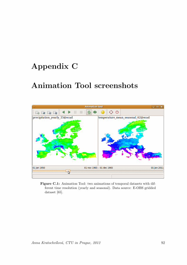
Appendix C

Animation Tool screenshots

Figure C.1: Animation Tool: two animations of temporal datasets with dif-ferent time resolution (yearly and seasonal). Data source: E-OBS griddeddataset [65].


Chapter C. Animation Tool screenshots

Figure C.2: Animation Tool: synchronized 2D and 2.5D animation of thesame area using multiple maps without time information. Data source:NagsHead mapset [54]

Figure C.3: Animation Tool: dialog for defining animation properties


Chapter C. Animation Tool screenshots

Figure C.4: Animation Tool: dialog for exporting animation — adding dec-orations

Figure C.5: Animation Tool: dialog for adjusting speed of animation (tem-poral mode active)


czech technical university in prague faculty of civil...

Documents