cyclic behavior in real estate_05

8/6/2019 Cyclic Behavior in Real Estate_05

http://slidepdf.com/reader/full/cyclic-behavior-in-real-estate05 1/21

Jin and Grissom 105

INTERNATIONAL REAL ESTATE REVIEW

2008 Vol. 11 No. 2: pp. 105 – 125

Forecasting Dynamic Investment Timing underthe Cyclic Behavior in Real Estate

Changha JinDepartment of Real Estate, J. Mack Robinson College of Business, Georgia StateUniversity, P.O. Box 4020, Atlanta, Georgia 30302-4020; Tel: (404) 413-7733, Fax:(404) 413-7736; E-mail: [email protected]

Terry V. GrissomSchool of the Built Environment, The University of Ulster, Jordanstown Campus,Shore Road, Newtownabbey Co. Antrim. UK BT 37, 01144-289-068-3794; E-mail:

[email protected]

This paper applies the Hodrck-Prescott (HP) filter to forecast short-termresidential real estate prices under cyclical movements. We separate thetrend component from the cyclical component. We show that each regionalresidential market reacts not only to previous price movements, but also thatthese regional markets react to previous shocks under Auto RegressiveIntegrated Moving Average (ARIMA) modeling. Using the S&P Case-ShillerHome Price Index, we compare our forecast to index values from theChicago Mercantile Exchange (CME) Housing Futures and Options. Ourstudy identifies possible systematic errors from the different priceadjustments reflecting current market situations.

Keywords

Real estate investment; Real estate cycle; residential housing futures contract; Realestate risk hedging



106 Jin and Grissom

1. Introduction

Although real estate has been regarded as an asset class for investment in various

previous research papers, it does not have the appropriate hedging tool to account forits own risk. This conditional state is especially evident in dealing with residentialproperties as noted by Shiller (2003). In comparing securities markets with a broaddelineation of risk, he determines that the major risk to individuals is their potentialloss of income and their expenditures on housing. The latter exposure may occur aseither deficient flows or wealth erosion. He further notes that despite the potentialfrequency and magnitude of loss that can be encountered, no readily availablehedging devises or strategies are available or operating.

The Chicago Mercantile Exchange (CME) has created an innovation enablinghedging tool that provides derivative products such as futures and options to hedgerisk in the residential real estate that is available. As more sophisticated risk-hedgingtools are developed, there will be an increasing demand to accurately forecastfluctuations in the real estate market. Accurately forecasting the future price of housing, while considering aggregate market behavior, would offer substantialbenefits to both investors and owners seeking to hedge a major component of theirpersonal wealth.

Regarding cyclic behavior in the real estate market, it is generally assumed that realestate markets go through both physical and financial market cycles and that thesehave differing effects on property prices. Fisher, Hudson-Wilson, and Wurtzebach(1996) used comparative statistics to investigate the separate and integrated impactthat these cycles have on space and capital markets. Their work offers theoreticalfoundations for the cyclical descriptions promulgated by Mueller (1999) and othergeneralized studies of property cycles.

The recursive relationship between market structures and cycles is important to

understanding property markets and cycles as it allows a dynamic rather than acomparatively static approach to modeling and developing the analytics of property.Forecasting the accuracy of property markets cannot be separated from a market’scyclical patterns. However, the forecasting of cyclical behavior has been challenginggiven that real estate’s cyclic integration with the assumptions of pure marketefficiency is inconclusive in terms of the effects on pricing.

Differences in cyclic studies premised on housing market efficiencies have produceddifferent findings and conclusions in the literature. For instance, Case and Shiller

(1990) found that the residential housing market was not efficient in predictingannual changes in prices and tended to be followed by changes in the same directionas in the preceding year. This conflicts with the concept of rational expectations,which Gau (1987) contends is a primary assumption and the foundation of theefficient market hypothesis (EMH). Case and Shiller’s findings suggest thatresidential property markets are a function of adaptive expectations. The conjecture



Jin and Grissom 107

of adaptive expectations implies that knowledge of prior prices can influence currentprices, and this knowledge can help predict future price behavior.

In a similar context, Clapp and Giaccotto (1994) show evidence that housing pricesdo not quickly reflect publicly available information. Local unemployment statistics,expected levels of inflation, changes in mortgage rates, income levels, the averageage of the population, or other exogenous factors operate to offset “pure” adaptiveprice patterns. This suggests a possible lag and/or an endogenous affect on thedynamics of property prices.

Academic findings as to the occurrence of real estate market efficiency are stillinconclusive, and fundamental financial analysis remains the dominant approach

used to predict real estate market performance. As practiced, fundamental analysis isbased on a microeconomic framework that often employs macroeconomic variablesand policies that are applied using representative agent models. Variables are oftencombined to simulate cash flow measures. These include multiple inflationmeasures, volatility in mortgage interest rates, regional population and incomegrowth, and changes in money supplies and other capital market activities.

Analysts often use more complicated forecasting models than the parsimoniousmodel proposed in this study to characterize the effects of macroeconomic variables

as likelihood variables that best specify real estate asset and market behavior. Whileoffering exogenous likelihood models using the variables identified above, thetechnique usually used is often termed fundamental analysis. In this context, it tendsto concentrate on the variables quantifying systematic risk that do not fit the assetspecific measures that traditional fundamental analysis focuses on.

The following constraints challenge the validity of both types of fundamentalanalysis. First, the model must employ the right fundamentals with the rightspecifications and the right set of exogenous variables. It should then be able to

forecast the economic variables included in the model. The forecasts of thefundamentals must differ at least in part from those of the market. The model used inthis study is a reduced form, which offers a less complex alternative to thecomplicated forecasting models used by most analysts. Nevertheless, it still requiresthe consideration of an adaptive lagged relationship, which is difficult to identify.For this reason, it is subject to the dynamics of time variation.

This study applies analytics that focus on past prices while ignoring the exogenouseconomic and political factors characteristic of the arbitrage and fundamental

econometric model. In this context, successful modeling depends on the discovery of price patterns that repeat themselves or are within the range of expected amplitude.Variations in or the failure to comply with the criteria expected may assist inidentifying anomalies. Identification of anomalies requires further specializedinquiry. This study attempts to test for more sensitive forecasting models thatintegrate real estate cyclic behavior.



108 Jin and Grissom

2. Purposes of Research

The purpose of this study is to develop an alternative to the linear market models that

focus on systematic risk models. Assuming that the residential real estate market hasadaptive expectations of price patterns, we attempt to investigate endogenous timeseries components by focusing on trends and cyclical relationships withautoregressive structures and temporal lag patterns.

Hodrick – Prescott (1997) hypothesized that the growth component of aggregateeconomic time series would vary smoothly over time. We believe that an applicationof the Hodrick–Prescott (HP) filter to property is consistent with their conjecture thatthe real estate market – as major component of a macro-economy – will grow

smoothly over time.

Following the methodology adopted by Hodrick and Prescott, we attempt in thispaper to determine if cyclical behavior does, in fact, exist in residential markets. Byseparating the trend component from the cyclical component in the time series of prices using their filter, we attempt to achieve decomposition.

Another purpose of this research is to determine the best fitting model among theAuto Regressive Integrated Moving Average (ARIMA) models given the

endogenous adaptive expectations noted above. The ARIMA model selected isidentified by those that performed well in relatively short-term market predictions.The fit of the method selected supports the use of eight parsimonious models todecompose short-term cyclical series as created by Box-Jenkins. ARIMA-basedmodels have been widely used in short-term forecasts, which are likely a good fit foradaptive expectations. Support for the ARIMA methodology is consistent with theform of S&P/Case-Shiller housing price data and index. The S&P/C-S index is usedas a reference for CME housing futures and options. The index is designed to beupdated monthly using the transacted data from the previous three months.

The third purpose of this paper is to measure the systematic errors occurring betweenthe real estate cycle forecasting model suggested by this study and the actualoutcomes. The sample test logically follows the general rule for cash assessmentderived from CME housing futures transactions. Thus, the main study objective isnot to generate an optimal forecasting model, but rather to identify the systematicbehaviors of forecast errors estimated by variations between the forecast model andthe outcomes and observations of actual market fluctuations.

3. Literature Review

The real estate cycle has been the topic of a number of academic studies. Pyhrr,Webb, and Born (1990) provide a typical trend model for real estate analysis, with atheoretical cyclical model based on demand, supply, and inflation. Their conclusionson the benefits of real estate investment timing suggest an endogenous or inefficient



Jin and Grissom 109

market attribute with real estate assets benefiting from market timing. In this regard,they have, unlike securities markets, which are more exogenous, a more efficientmarket.

Pyhrr, Webb, and Born (1990) also compare traditional methods such as thetraditional correlation of inflation against a model using cyclical assumptions such asdemand, supply, absorption, occupancy rates, and rental rate differences betweennewly constructed and existing properties. They conclude that a cyclical model maybe a better indicator of investment value maximizing expected “real” returns incomparison to market value without taking inflation cycles into consideration. Thismeans that the real estate market cycle is based on its temporal position, which isdelineated by physical components. Changes in vacancy rates, rental prices, existing

stock, and new construction are all seen as cyclical descriptors of the market. Theyfurther suggest that the physical descriptors should be compared with financialcapital market factors.

With regard to the residential real estate market cycle, studies by Chinloy (1996) of multifamily housing in Tucson and Phoenix, Arizona, in the United States, suggestthat cycles are characterized by upside and downside lags of three years. Abrahamand Hendershott (1996) propose a model with housing prices appreciating along withequilibrium prices and the adjustment procedure in the equilibrium price process.

Capozza et al (2002) investigate the dynamics of housing prices using a time-seriesanalysis, which estimates serial correlations as well as means reversion parameters of the housing price index. They suggest that variations in the cyclical behavior of realhousing prices depend on variations in local economic variables along withconstruction costs and the growth rate of the metropolitan area.

Grissom and DeLisle (1999) find that the fluctuation characteristics of cycles can besegmented into temporally delineated economic regimes, which are defined asconsistent return behaviors that are associated with key systematic variables.Although the returns are consistent in the direction of the trends calculated with theuse of spline analysis, they delineate the segments of the splines linked to specificturning points. The direction of the returns is proven to be relative to the splines forthe span of a regime. The technical shifts that are conditional to these systematicvariables are used to designate inflection points that signify structural changes andfundamental relationships. The regimes represent long-term structural trends, whichenable the separation of return cycles that characterize unsystematic components of property assets in time.

Using short-term cyclical behavior, Witkiewicz (2002) examines the use of the H-Pfilter to identify the impact of indicators on the real estate cycle. Similarly, Matysiak,and Tsolacos (2003) attempt to investigate short-term cycles in office rental marketsand their leading relationship with other macro-economic variables. They also applyH-P filters to isolate the sensitivity of a rental index to corresponding economicvariables. Crawford and Frantantoni (2003) construct invariant time series modelsfor housing prices. This technique allows for a comparison of the forecasts of home



110 Jin and Grissom

price changes using three techniques: an ARIMA model, a Generalized AutoRegressive Conditional Heteroskedasticity (GARCH) model, and a Regime-Switching model. Crawford and Frantontoni (2003) conclude that while regime-

switching models tend to perform better in sample studies, the ARIMA modelsgenerally forecast better in terms of short-term predictions.

4. Data and Methodology

The period under study runs from January 1987 to October 2006. Data were drawnfrom the S&P/Case-Shiller Home Price Index, which was launched in May 2006 bythe CME to provide information on price housing futures and options on residential

housing markets in 10 metropolitan regions across the United States. It is calculatedmonthly, using three-month moving average tracking data. Its value for each monthis based on sales pairs found for that month and the preceding two months.

The H-P filter is widely used by macroeconomists to obtain a smooth estimate of thelong-term trend component of a series. We use it to identify short-term cyclicalbehavior and long-term trends The deviation of this trend from the actual rental valueis defined as the short-term cyclical volatility. We use the H-P filter specificationproposed by Witkiewicz (2002). In this form, the filter is useful for decomposing a

time series, , into a cyclical component, , and a trend component ,t y ct y gt y

= + (1)t y ct y g

t y The HP-filter sets the minimization of variance of the cyclical component subject toa penalty constraining the variation by the second difference of the growthcomponent. Thus, the method results in solving the following minimization problem:

(2)∑=

−++

= −−−+−=T

t

gt

gt

gt

gt

gt t

T t

gt y y y y y y y

1

211

210 ])]()[()[(min}{ λ

where λ controls the smoothness of the series by penalizing the growth component,gt y

The first order condition from the minimization problem results in

The first order condition for is given by

gt t y L L y ])1()1(1[ 212 −−−+= λ

ggt y L H y )(=

(3)

t

1212 ])1()1(1[)( −−−−+= L L L H g λ (4)

where L is the lag operator and the cyclical component, where

(5)t c

t gg

t t ct y L H y L H y y y )())(1( =−=−=

HP(L) is given by:t y

42

42

22

42

212

212

)1() / 1()1(

)1(1)1(

]1[]1[1]1[]1[

)( L L

L L L L

L L L L

L L L HP c

−+

−=

−+

−=

−−+

−−=

−

−

−

−

−

−

λ λ λ

λ λ

(6)



Jin and Grissom 111

As λ approaches infinity, the growth component approaches a trend line.gt y

Hodrick and Prescott (1997) recommend that λ = 100 for annual data, 1,600 for

quarterly data, and 14,400 for monthly data. In this study, the frequency power rulemethodology was suggested by Ravan and Uhlig (1997).

All regional series are filtered to remove the long-term trends and isolate the cyclicalcomponents of the series. The cycles obtained from this procedure are then used asinput for forecasting. The first step of the analysis decomposes the long-term trendand short-term cycle.

Table 1 presents descriptive statistics for long-term trends and short-term cycles for

the 10 regions traded in CME real estate futures and options. The calculation showsthat Las Vegas, Nevada; San Diego, California; Los Angeles, Califonria; and Miami,Florida, have a higher standard deviation on short-term cycles while San Diego, LosAngeles, Miami, and San Francisco, California, have greater fluctuations in long-term trends.

The short-term analysis used for technical modeling is critical because the periodicadjustments needed for indexing require monthly data measurements using analgorithm for a three-month moving average. To forecast the effects of the short-termcycle, we apply an ARIMA model. The ARIMA model contrasts directly with themethodology of property analysts, who use fundamental analysis based onexogenous economic variables. ARIMA models are generalizations of the simple ARmodel, which uses the following tools for modeling the serial correlation in thedisturbance.

ARIMA’s first component is the autoregressive or AR term. Each AR termcorresponds to the use of a lagged value in the forecasting equation. Therefore, thelagged value can reflect the current market situation. An autoregressive model of order p , AR ( p) has the form:

t pt pt t t y y y y ε β β β ++++= −−− ...221 (7)

The second component is the moving average (MA) term. With an MA, theforecasting model uses lagged values of the forecast error to improve the currentforecast. A first-order moving average term uses the most recent forecast error; asecond-order term uses the forecast error from the two most recent periods, and soon. The error can reflect any newly introduced shocks to current housing markets.The MA ( q) has the form:

t qt qt t t y ε ε θ ε θ ε θ ++++= −−− ...221 (8)

Thus, the auto regressive and moving average specifications can be combined toform an ARMA ( p,q ) specification:

t qt qt t t pt pt t t y y y y −−−−−− ++++++++= ε θ ε θ ε θ ε β β β ...... 221221 (9)



112 Forecasting Dynamic Investment Timing Under Cyclic Behavior

Table 1 Descriptive Statistics for Long-term Trends and Short-term Cycles

Short term Cycle Mean Max Min Std. Dev. Skewness Kurtosis Mean Beginning

Boston 2.92E-11 5.88 -7.23 1.89 -0.18 4.48 99.41 64.60

Chicago 3.95E-10 4.34 -4.62 1.56 0.17 3.72 96.85 58.17

Denver 2.55E-10 6.80 -4.71 2.35 0.62 3.37 84.70 48.11

Las Vegas 3.84E-10 23.48 -20.47 7.28 -0.18 5.61 107.86 64.30

Los Angeles 2.85E-10 15.43 -12.32 6.08 0.18 2.54 114.39 67.39

Miami 3.26E-10 20.41 -13.47 5.45 1.11 7.52 112.54 70.17

New York 4E-10 8.23 -8.53 2.52 -0.05 4.55 106.68 75.67

San Diego 2.85E-10 20.99 -22.66 6.24 0.73 5.28 111.09 58.16

San Francisco 3.74E-10 15.18 -10.87 5.38 0.71 3.44 100.63 50.85

Washington 3.79E-10 18.49 -14.84 4.94 0.94 6.23 115.41 71.59

Note : Begins January 1987 and ends October 2006. The data are on sales of specific single-family homes. Each sspecify for smoothing parameter, λ , the study followed the method suggested by Ravan and Uhlig (200




The method applied for short-term cyclic behavior is a function of the AR and MAprocesses. On the one hand, the AR represents the behavior of current values asfunctions of recent past values. The technique to decompose the MA component, on

the other hand, provides the processes in which past innovations continue toreverberate for a number of periods. The study follows the structure of the Box-Jenkins model. This model allows for a choice of lagged variables to maintain thedegrees of freedom.

5. Results

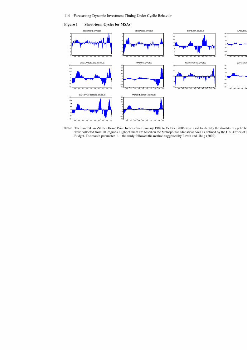
As examples, Figures 1 and 2 show the short-term cycles and long-term trends,

respectively, in Los Angeles after applying the H-P filter. The fluctuations of short-term cycles are detected from 1988 to 1990 and from 2003 to 2005 over most of theregions included in the study. The up-cycles observed in the late 1980’s areassociated with the massive speculation in construction that peaked in 1989-1990.The market started to slide in the early 1990’s for both residential and commercialproperties until vacancy exceeded 30% nationwide. Throughout the 1990’s, the realestate market experienced largely increasing development, with the nationwideinventory nearly tripling. In the up-cycle of the early 2000’s, there were increasingconcerns about the development of a national real estate bubble.

The traditional observations and the implications of past occurrences support theapplication of two forecasting techniques in the specification of trends and cycles.An exponential smoothing technique is applied in this study to forecast long-termtrends. This approach is utilized because the trend decomposed using the HP filtersshows stability to be positive and on an upward graphical pattern. The secondapproach used for short-term cycles is the ARIMA models. Unit root testing isconsidered to be the first stage for ARIMA modeling to check whether the absolutevalue of the parameter is less than one. The unit root results are reported in Table 2.

The test data reveal strong evidence of stationary conditions in the short-term cycleseries. The study shows that eight of the 10 regions are significant at the 1% level inthe Augmented Dickey-Fuller test. Los Angeles and San Diego are exceptions, beingsignificant at the 5% level. In addition, most regions exhibit strong evidence of astationary condition at the 5% level in the Phillips – Perron test. While a popularapproach for testing the stationary condition involves carrying out consecutivedifferencing on the data series and then fitting the ARIMA model to them, the short-term cycles are enough to confirm the stationary condition without a differencing

process. Therefore, the strict model definition in our study necessarily applies theAuto Regressive Moving Average Model (ARMA) as a stringent methodology term.

As a model selection rule, we employ the Akaike Information Criterion (AIC) toensure that the most accurate model is selected from the class of eight possiblemodels suggested by the Box-Jenkin’s methodology. In Table 3, four models aresorted and selected using the AIC criteria.




Figure 1 Short-term Cycles for MSAs

-8

-6

-4

-2

0

2

4

6

88 90 92 94 96 98 00 02 04 06

BOSTON_CYCLE

-6

-4

-2

0

2

4

6

88 90 92 94 96 98 00 02 04 06

CHICAGO_CYCLE

-6

-4

-2

0

2

4

6

8

88 90 92 94 96 98 00 02 04

DENVER_CYCLE

-15

-10

-5

0

5

10

15

20

88 90 92 94 96 98 00 02 04 06

LOS_ANGELES_CYCLE

-15

-10

-5

0

5

10

15

20

25

88 90 92 94 96 98 00 02 04 06

MAIAMI_CYCLE

-10

-5

0

5

10

88 90 92 94 96 98 00 02 04

NEW_YORK_CYCLE

-12

-8

-4

0

4

8

12

16

88 90 92 94 96 98 00 02 04 06

SAN_FRANCISCO_CYCLE

-16-12

-8

-4

0

4

8

12

16

20

88 90 92 94 96 98 00 02 04 06

WASHINGTON_CYCLE

Note: The SandP/Case-Shiller Home Price Indices from January 1987 to October 2006 were used to idenwere collected from 10 Regions. Eight of them are based on the Metropolitan Statistical Area as deBudget. To smooth parameter, λ , the study followed the method suggested by Ravan and Uhlig



Figure 2 Long –Term Trend for MSAs

60

80

100

120

140

160

180

200

88 90 92 94 96 98 00 02 04 06

BOSTON_TREND

40

60

80

100

120

140

160

180

88 90 92 94 96 98 00 02 04 06

CHICAGO_TREND

40

60

80

100

120

140

160

88 90 92 94 96 98 00 02 04 06

DENVER_TREND

40

80

120

160

200

240

280

320

88 90 92 94 96 98 00 02 04 06

LOS_ANGELES_TREND

40

80

120

160

200

240

280

88 90 92 94 96 98 00 02 04 06

MAIAMI_TREND

40

80

120

160

200

240

88 90 92 94 96 98 00 02 04 06

NEW_YORK_TREND

40

80

120

160

200

240

88 90 92 94 96 98 00 02 04 06

SAN_FRANCISCO_TREND

40

80

120

160

200

240

280

88 90 92 94 96 98 00 02 04 06

WASHINGTON_TREND

Note: The SandP/Case-Shiller Home Price Indices from January 1987 to Octover 2006 were used to ideThe data were collected from 10 Regions. Eight of then are based on the Metropolitan Statistical AManagement and Budget. To specify for smoothing parameter, λ , the study followed the meth




Table 2 Unit Roots Test for Short-term Cycles

ADF Test PP Testt-statistic p-value t-statistic p- value

Boston -5.256* 0.000 -3.378* 0.001

Chicago -5.017* 0.000 -3.876* 0.000

Denver -3.979* 0.000 -1.995** 0.044

Las Vegas -4.125* 0.000 -2.784* 0.005

Los Angeles -2.479** 0.013 -2.544** 0.011Miami -5.883* 0.000 -2.700* 0.007

New York -3.494* 0.001 -3.737* 0.000

San Diego -1.934** 0.050 -2.032** 0.041

San Francisco -3.527* 0.001 -2.886* 0.004

Washington -3.505* 0.001 -2.832* 0.005

Note: Augmented Dickey- Fuller test statistic (ADF), Phillips-Perron test statistic (PPtest)* and ** indicate significance at the 1% and 5% levels.

Table 3 shows that the ARMA (2, 2) model is the best forecasting model for Boston,Massachusetts; Los Angeles; Miami; New York, New York; San Francisco, andWashington, DC. The ARMA (1, 2) model is the best predictive structure inChicago, Illinois, and ARMA (2, 1) model achieves the appropriate forecastingstructure for Las Vegas. The simpler AR (2) with 2 short-term lag offers anappropriate forecasting procedure for Denver, Colorado, and San Diego.

Forecasting out-of-sample periods (2005 1Q – 2006 3Q) are presented in Table 4.We constructed the forecast index from two components: short-term cycle forecastsgenerated by the best-fitting model from Exhibit 5 and the long-term trend forecastsgenerated by double exponential smoothing. The monthly forecasts are shown for theperiod from April 2005 to October 2006. However, to make things smple, we onlypresent four data points per year with monthly data observations. The magnitude of error can be realized from the inequality between the actual index observed and theforecast index constructed. The last column in Table 4 shows the dollar amount of

gains and losses from the magnitude of error in forecast models with associated cashassessment.




Table 3 Alternative ARIMA Models1 β AIC 1 β

Boston miMiaARMA(2,2) 1.210* -0.358* 0.525* 0.579* 1.214 ARMA(2,2) 1.695* ARMA(1,2) 0.864* 0.825* 0.685* 1.232 AR(2) 1.777*AR(2) 1.614* -0.721* 1.419 AR(1) 0.989*ARMA(2,1) 1.616* -0.724 -0.006** 1.427 MA(1) Chicago New York ARMA(1,2) 0.859* 0.620* 0.543* 0.891 ARMA(2,2) 1.498 *ARMA(2,2) 0.873* -0.015* 0.602* 0.538* 0.894 AR(2) 1.809* AR(2) 1.451* -0.527* 1.014 ARMA(2,1) 1.798*ARMA(2,1) 1.513* -0.586* -0.085* 1.018 MA(1) Denver San Diego

AR(2) 1.658* -0.679* 0.414 AR(2) 1.845ARMA(2,1) 1.687* -0.707* -0.050* 0.420 ARMA(2,1) 1.871* MA(2) 1.413* 0.893* 2.357 MA(2) MA(1) 0.936* 3.331 MA(1) Las Vegas San FranciscoARMA(2,1) 1.832* -0.858* -0.013* 2.151 ARMA(2,2) 1.697*ARMA(1,1) 0.983* 0.652* 2.725 ARMA(2,1) 1.805*MA(2) 1.429* 0.969* 4.539 AR(2) 1.855*MA(1) 0.989* 5.497 MA(1) Los Angeles WashingtonARMA(2,2) 1.760* -0.787* 0.148* 0.370* 1.337 ARMA(2,2) 1.764AR(2) 1.858* -0.881* 1.468 ARMA(2,1) 1.846*ARMA(2,1) 1.839* -0.863* 0.075** 1.469 MA(2) MA(1) 0.981* 5.132 MA(1)

Note : AIC results for the alternative ARMA models over the estimation period. The lower the statistic the better the mo* and ** indicate significance at the 1% and 5% levels, respectively. The best fitting model are in bold fo




Table 4 Performance of Forecast Index and S&P/CS

PeriodForecastTrends

(T)

ForecastCycles

(C)

ForecastIndex(FI)

S&P/CS ForecastError (FE)

Dollaramount of gains and

losses

(Trend) (Cycle) (FI=T+C) (SPCS) (FI-SPCS) (FE/0.2)*$250

Boston2005 1Q 173.33 0.677 174.01 174.76 -0.751 -$1,000

2Q 175.35 4.865 180.22 181.17 -0.954 -$1,2503Q 177.09 4.491 181.58 181.67 -0.088 $04Q 178.58 3.114 181.70 181.69 0.006 $0

2006 1Q 179.88 -2.528 177.35 176.27 1.084 $1,2502Q 181.07 -2.151 178.92 178.61 0.307 $5003Q 182.20 -4.213 177.99 175.72 2.268 $2,750

Chicago2005 1Q 150.57 0.263 150.84 151.02 -0.184 -$250

2Q 153.47 0.356 153.82 154.72 -0.897 -$1,0003Q 156.37 1.815 158.19 157.81 0.375 $5004Q 159.28 2.038 161.32 162.44 -1.121 -$1,500

2006 1Q 162.19 2.696 164.89 164.67 0.218 $2502Q 165.10 1.255 166.36 166.61 -0.251 -$2503Q 168.01 0.727 168.74 167.99 0.751 $1,000

Denver2005 1Q 134.36 -1.913 132.45 132.63 -0.182 -$250

2Q 135.44 -0.695 134.75 134.82 -0.073 $03Q 136.51 0.576 137.09 137.19 -0.101 -$2504Q 137.58 0.274 137.85 137.53 0.319 $500

2006 1Q 138.63 -1.142 137.49 137.12 0.369 $5002Q 139.68 -2.018 137.66 138.31 -0.645 -$7503Q 140.73 0.158 140.89 140.27 0.623 $750

Las Vegas2005 1Q 194.39 12.649 207.04 209.31 -2.271 -$2,750

2Q 201.91 15.553 217.46 217.28 0.183 $2503Q 209.44 14.201 223.64 224.51 -0.868 -$1,0004Q 216.97 11.885 228.85 228.77 0.083 $0

2006 1Q 224.48 7.018 231.50 231.94 -0.440 -$5002Q 231.98 3.212 235.20 234.39 0.806 $1,0003Q 239.48 -4.327 235.15 234.78 0.370 $500

(Continue...)



Jin and Grissom 119

Table 4 Continued


(T)

ForecastCycles

(C)

ForecastIndex(FI)


Dollar

amount of gains andlosses


L A2005 1Q 221.23 0.390 221.62 222.29 -0.672 -$750

2Q 230.00 6.346 236.34 236.68 -0.338 -$5003Q 238.82 11.709 250.53 251.1 -0.573 -$7504Q 247.67 16.301 263.97 262.56 1.406 $1,750

2006 1Q 256.52 10.643 267.16 267.75 -0.586 -$7502Q 265.37 6.961 272.33 272.12 0.214 $2503Q 274.22 0.180 274.40 273.8 0.601 $750

Miami2005 1Q 214.15 -4.754 209.40 209.67 -0.275 -$250

2Q 223.27 3.749 227.01 227.10 -0.085 $03Q 232.52 11.447 243.97 245.24 -1.272 -$1,5004Q 241.87 19.961 261.83 261.00 0.826 $1,000

2006 1Q 251.26 19.959 271.22 271.68 -0.463 -$5002Q 260.67 17.619 278.29 278.68 -0.390 -$5003Q 270.09 8.141 278.23 276.80 1.430 $1,750

New York 2005 1Q 187.12 2.117 189.24 189.29 -0.048 $0

2Q 192.32 3.432 195.75 195.96 -0.209 -$2503Q 197.52 4.363 201.88 202.33 -0.447 -$5004Q 202.72 7.321 210.04 210.30 -0.261 -$250

2006 1Q 207.91 5.925 213.83 214.47 -0.636 -$7502Q 213.09 2.536 215.63 215.59 0.036 $03Q 218.26 -3.679 214.58 214.01 0.574 $750

San Diego2005 1Q 221.41 13.015 234.42 235.64 -1.219 -$1,500

2Q 228.37 13.882 242.25 242.00 0.248 $2503Q 235.25 13.833 249.08 248.45 0.633 $7504Q 242.06 8.503 250.57 250.34 0.226 $250

2006 1Q 248.82 -2.019 246.80 247.89 -1.089 -$1,2502Q 255.54 -4.736 250.80 249.15 1.654 $2,0003Q 262.24 -13.177 249.06 247.30 1.765 $2,250

(Continue...)



120 Jin and Grissom

Table 4 Continued


(T)

ForecastCycles

(C)

ForecastIndex(FI)


Dollar

amount of gains andlosses


San Francisco2005 1Q 189.08 3.907 192.99 193.50 -0.513 -$750

2Q 194.40 10.175 204.58 205.52 -0.943 -$1,2503Q 199.74 13.730 213.47 212.86 0.607 $7504Q 205.07 11.121 216.19 215.70 0.490 $500

2006 1Q 210.39 4.384 214.77 215.50 -0.727 -$1,0002Q 215.70 3.383 219.08 218.37 0.711 $1,0003Q 221.00 -3.562 217.44 217.23 0.208 $250

Washington2005 1Q 208.60 2.512 211.11 212.24 -1.128 -$1,500

2Q 216.07 13.835 229.90 229.87 0.031 $03Q 223.56 19.175 242.73 242.06 0.671 $7504Q 231.04 15.436 246.48 246.70 -0.219 -$250

2006 1Q 238.52 9.391 247.91 248.39 -0.479 -$5002Q 245.98 5.950 251.93 251.13 0.800 $1,0003Q 253.43 -3.644 249.78 248.17 1.613 $2,000

Note : S&P/CS represents S&P/Case Shiller home price indices. Dollarization follows the CMEFutures contract rule in terms of minimal increments called "ticks" with the value of 0.20index point, and $250 as a product multiplier. Therefore, 0.20 of differences in two indexvalues cause $250 x 0.20 =$50.0 gains or losses for investors holding short future position.The quarter presented in Table follows the CME trading month (February, May, August,and November) except 3rd quarter of 2006. Oct 2006 replaced the 3rd quarter basis. ForShort-term cycles, the best model selected from table 3 was applied to forecast the series.

Double exponential smoothing method was applied for Long-term trend.

Table 4 follows the transaction process used in the CME housing futures marketwhen an investor sells one future contract at the forecast index value. The unit of change is derived by comparing the CME method, with errors observed by theforecast being adjusted by 0.2. This adjustment is consistent with the minimum unitchanges in CME housing futures. The contract is valued at $250, which is the samevalue applied in a CME housing futures contract. Thus, the best forecast model is themodel that yields the cumulative error closest to zero where the dollar amount of gains and losses is closest to zero. In addition, the forecast errors can explain theamount of divergence from rational expectation based on previous existing marketinformation and the reflection of additional shocks. Therefore, the pattern and insightgained from the forecast errors will contribute to proper investment timing. If thereal estate market is fundamentally efficient, the fluctuation of current market



Jin and Grissom 121

estimates can be expected to converge toward the actual value of moderate marketconditions without any additional shocks taking place in the expected model.

The generated series, the differences between the forecasted model, and the referenceindex show that there is a consistent pattern and cyclical behavior. The changes inmarket direction are observed in subsequent periods, and decay is on a serial basis.The negative forecast errors in out-of-sample data are captured in the housing priceindex beginning in early 2005. We find that a cyclical behavior in negative forecasterror that started in the previous month increasingly occur in subsequent months. Thus, even though the forecast model is weak in identifying a large upward ordownward movement, changes in the number of forecast errors will provideinformation on market direction. They will also yield further insight regarding

investment timing.In Table 4, if the value of the S&P/CS index for Los Angeles was reported as 222.2in the first quarter of 2005, the contract value would equal $55,550 (= $250 x 222.2).The negative forecast error would result in a $750 loss on the futures transaction.The negative forecast errors observed in the first quarter of 2005 would be followedin subsequent periods with a loss of $500 in the second quarter of 2005 and a loss of $750 in the third quarter. The negative forecast errors would occur when the realS&P C-S index increased to a value that was higher than expected from the forecast

index for Boston, Chicago, Los Angeles, Miami, New York, and San Francisco.These regions were suspected of having potential housing bubbles in late 2004 andearly 2005.

In up-markets, the forecast model calls for conservative guidelines. This could be theresult of real market movements that exceeded the market forecasts, which, in turn,would result in cash losses for CME futures contracts. This would occur whenmarket demand increases as the trading volume increases. In this case, the forecastmodel would systematically project lower forecasting values than the real outcomefrom S&P Case Shiller index. As shown in early 2005, most regions would havelosses on CME futures contracts if guided by our forecast model. These systematicnegative errors occur in up-markets or seller’s markets, when the bid prices offeredby buyers rapidly move to the seller’s asking price because of increased tradingvolumes.

While consecutively negative additive or multiplicative errors are observed in up-markets, negative additive errors have also occurred in down-markets such as inearly 2006. Most regions have positive cash values on selling a future contract whenguided by our forecast. These systematic negative errors are typically observed indown-markets or buyers’ markets, when the asking prices offered by sellers rapidlymove to the buyer’s bid price owing to lower trading volumes. The additive ormultiplicative errors observed in down-markets can be attributed to these systematicnegative errors. Thus, the test results suggest that once a real estate market passes theturning point, the pattern shows serially additive or multiplicative movement.



122 Jin and Grissom

6. Conclusion

Various prior studies have regarded real estate as a distinct asset class for

investment. However, unlike other financial asset classes, real estate does not haveappropriate exogenous hedging tools to reduce the risk. As with other financial assetclasses, risk-hedging tools are offered for real estate through the housing derivativeprogram of the Chicago Mercantile Exchange (CME). Demand for relative short-term forecasts is expected to increase as the housing derivative market expands.

This study has compared the validity of the forecasting model constructed for 10regions across the United States. The H-P filtering technique was applied to test forsensitive forecasting models incorporating real estate cyclical behavior and market

reflection by decomposing the trend component of aggregated market growth fromthe cyclical component in a time series. The study used the decomposed short-termcyclical series as an alternative to ARIMA modeling. The results show that althoughthe ARIMA model is limited to identifying large upward and downward changes, itdoes sufficiently capture the market direction and pattern of the systematic errorspresented in Table 5. The study further shows that the forecast errors decayedserially and expanded additively while the amount of forecast errors stated inprevious months has also occurred in subsequent observations.

Although the main purpose of this study was not to generate an optimal forecastingmodel, these systematic behaviors from errors estimated by forecast model and realmarket fluctuation will be useful for designating a market proxy that adequately fitsthe needs of hedging loss exposure for investors interested in market timing. Whilethe forecasting developed within data from the prior month impact subsequentobservations, the effects reflect an additive pattern with the autoregressive andmoving average effects are consistent with adaptive expectation.

Though the proxy time series model in this study is a reduced form model of a highly

complex situation, significant insights can be derived from it. Market timing inresidential properties can significantly impact investor benefits, but these benefits atany given point in time would have a relatively short-term impact.

Given the relevance of market timing to the residential property market, appropriateforecasting techniques would have to consider the use of adaptive explanations as astraightforward form of the local property market. This study accepted a modelingconjecture of AR and supported the quantitative equipment of AR and MAcomponents in the Box Jenkins tradition of time series analysis. This study also

employed theoretically premised quantitative techniques to decompose time seriesinto a cyclical as risk component as variance around a relatively defined short onlong term growth trend enables insights to assist hedging to cover the significant risk exposure to housing expenditure.

The implication of adaptive pricing expectation from endogenous variables also setsa foundation for future research into decomposed patterns to identify useful



Jin and Grissom 123

indicators related to the real estate market. Future research is needed to adopt usefulindicators related to the real estate market. The economic variables will also be ahelpful tool for forecasting market turning points only if they can play a role as a

leading indicator.

Acknowledgements

The authors gratefully acknowledge the financial support for this research from theDepartment of Real Estate at the Robinson College of Business at Georgia StateUniversity. We would also like to acknowledge the insightful comments from theparticipants at the 2007 American Real Estate Society annual academic conferenceand Professor Alan Ziobrowski. This paper received the 2007 Best Research Paperon Real Estate Finance award, sponsored by the Fannie Mae Foundation andpresented at the 2007 ARES Annual Meeting.

References

Case, K. and Shiller, R. (2003). Is there a bubble in the housing market? BrookingsPapers on Economic Activity, (2), 299-362.

Capozza, D., Hendershott, P., Mack, C., and Mayer, C. (2002). Determinants of realhouse price dynamics. NBER Working Paper Series , No. 9262.

Chicago Mercantile Exchange (2006). CME housing futures and optionsintroductory guide. Retrieved March 10, 2007, fromhttp://www.cme.com/files/cmehousing_brochure.pdf

Chinloy, P. (1996). Real estate cycles and empirical evidence. Journal of Housing Research , 7, 173–190.

Clapp, J. and Giaccotto, C. (2002 ). Evaluating house price forecasts. Journal of Real Estate Research, 24 (1), 1-16.

Clayton, J. (1996). Rational expectations, market fundamentals and housing pricevolatility, Real Estate Economics, 24 (4), 30.

Crawford, G. and Michael, C. (2003). Assessing the forecasting performance of regime-switching, ARIMA and GARCH models of houses prices. Real Estate

Economics, 31 (2), 21.

http://www.cme.com/files/cmehousing_brochure.pdf





124 Jin and Grissom

Grissom, T. and Delisle, J. (1999). A multiplex index analysis of real estate cyclesand structural change. Journal of Real Estate Research , 18 (1), 33.

Grissom, T., Wang, K., and Webb, J. (1991). The spatial equilibrium of intra-regional rates of return and the implications for real estate portfolio diversification. Journal of Real Estate Research, 7 (1), 59.

Hodrick, R. and Prescott, E. (1997). Postwar U.S. business cycles: An empiricalinvestigation. Journal of Money, Credit and Banking, 29 (1), 1-16.

Matysiak, G. and Tsloacos, S. (2003). Identifying short-term leading indicators forreal estate rental performance. Journal of Property Investment and Finance, 21 (3),

20.Mueller, G. (1999). Real estate rental growth rates at different points in the physicalmarket cycle. Journal of Real Estate Research, 18 (1), 20.

Pyhrr, S., Born, W., Manning, C., and Roulac, S. (2003). Project and portfolioManagement decisions: A framework and body of knowledge model for cycleresearch. Journal of Real Estate Portfolio Management, 9 (1), 16.

Pyhrr, S., Born, W., and Webb, J. (1990). Development of a dynamic investmentstrategy under alternative inflation cycle scenarios. Journal of Real Estate Research,5 (2), 17.

Witkiewicz, W. (2002). The use of the HP-filter in constructing real estate cycleindicators. Journal of Real Estate Research, 23(1/2), 65.



Jin and Grissom 125

Appendix

Table 1A Metro Areas for the Original 10 S&P/Case-Shiller Home Price Indices*

MSA Represented Counties

1 Boston Essex MA, Middlesex MA, Norfolk MA, Plymouth MA, Suffolk MA,Rockingham NH, Strafford NH

2 Chicago Cook IL, Dekalb IL, Du Page IL, Grundy IL, Kane IL, Kendal IL,McHenry IL, Will IL

3 Denver Adams CO, Arapahoe CO, Broomfield CO, Clear Creek CO, DenverCO, Douglas CO, Elbert CO, Gilpin CO, Jefferson CO, Park CO

4 Las VegasClark NV

5 Los Angeles Los Angeles CA, Orange CA

6 Miami Broward FL, Miami-Dade FL, Palm Beach FL

7 New York City

Fairfield CT, New Haven CT, Bergen NJ, Essex NJ, Hudson NJ,Hunterdon NJ, Mercer NJ, Middlesex NJ, Monmouth NJ, Morris NJ,Ocean NJ, Passaic NJ, Somerset NJ, Sussex NJ, Union NJ, Warren NJ,Bronx NY, New York NY, Orange NY, Putnam NY, Queens NY,Richmond NY, Rockland N, Suffolk NY, Westchester NY, Pike PA

8 San Diego San Diego CA9 San Francisco Alameda CA, Contra Costa CA, Marin CA, San Francisco CA, San

Mateo CA

10 Washington

District of Columbia DC, Calvert MD, Charles MD, Frederick MD,Montgomery MD, Prince Georges MD, Alexandria City VA, ArlingtonVA, Clarke VA, Fairfax VA, Fairfax City VA, Falls Church City VA,Fauquier VA, Fredericksburg City VA, Loudoun VA, Manassas CityVA, Manassas Park City VA, Prince William VA, Spotsylvania VA,Stafford VA, Warren VA, Jefferson VA

Source : Standard & Poor’s Data Web Site

cyclic behavior in real estate_05

Documents