000CY)

~OF

DEPARTMENT OF THE AIR FORCE

AIR UNIVERSITY

AIR FORCE INSTITUTE OF TECHNOLOGY

Wright-Patterson Air Force Base, Ohio

AFIT/GA/ENY/9 1M-01 /

'y

EFFECTS OF COLOCATION AND NON-COLOCATEONOF SENSORS AND ACTUATORSON FLEXIBLE STRUCTURES

THESIS

W. C. LEE, Captain, USAF

AFIT/GA/ENY/9 IM-01

Approved for public release; distribution unlimited.

91-057431 " "~~~ ~~~~~~'ll Ii i~ ll I ill 11 l I

March 1991 Master ThesisEffect of Colocation and

Non-colocation of Sensors and Actuatorson Flexible Structures

W. C. Lee, Capt, USAF

Air Force Institute of Technology AFIT/GA/ENY/91M-01WPAFB, OH 45433-6583

Approved for public release;distributionunlimited

This thesis compares the performance and robustnessof colocated and non-colocated sensor/actuator pairs. Linear quadraticGaussian and loop transfer recovery (LQG/LTR) procedures are used todesign optimum controllers for three example problems. The firstexample is a single motion degree-of-freedom system having motion onlyabout one axis. This type of system does not have any right half planezeros for the non-colocated case;however, the thesis shows it behaves asa non-minimum phase system. The second example is a Bernoulli-Eulerbeam which does have RHP zeros. An optimum LQG/LTR controller can notimprove the robustness of non-minimum phase systems;whereas, colocatedsystems are aisy stabilize and make robust with LTR. However, thisthesis shows that non-colocated systems can achieve higher bandwidthand performance. So, each system has its own advantage.

control theory flexible qtructurcs, actuators, LQG/LTR

unclassified unclassified uncl .;sified unlimited

AFIT/GA/ENY/91M-01

EFFECTS OF COLOCATION AND NON-COLOCATIONOF SENSORS AND ACTUATORSON FLEXIBLE STRUCTURES

THESIS

Presented to the Faculty of the School of Engineering

of the Air Force Institute of Technology

Air University

In Partial Fulfillment of the

Requirements for the Degree of

Master of Science in Astronautical Engineering

W. C. Lee, B.S.C.E. /

Captain, USAF .

March 1991

Approv'ed for public release; distribution unlimited.

Acknowledqements

I wish to thank Mr Dan Malwitz of Contraves USA for

providinq the finite element model used in this thesis. He

was very helpful in clarifying questions I had concerning

finite element modeling and providing supporting materials.

Another group who deserves much thanks is the people at

Engineering Methods, Inc. of West Lafayette, Indiana. From

Luanna Hellerger, Paul Hunckler and Dave Phillips to Dr.

Charles Hunckler, I can not appreciate the amount of time and

effort they took to assist me in getting ANSYS up and running.

Also, Mr Bob Jurek and Mr Larry Falb at ASD's Scientific and

Engineering Applications Division were very helpful in getting

an account set up so I could use the commercial version of

ANSYS for some of my computer runs. I also appreciate the

contributions of the in-house people here at AFIT's computer

support and Capt Howard Gans in getting ANSYS set up in our

own laboratory. Finally, I need to thank Dr Patrick Sweeney

and Mr Tom Davis from University of Dayton who provided the

initial support in my using ANSYS as a research tool.

My deepest appreciation goes toward my thesis advisor, Dr

Brad Liebst, for his motivation and support during this thesis

effort. His patience and dedication to higher learning

allowed me to leave AFIT with a feeling of accomplishment in

ii

having learned a little about the new and exciLing field of

control engineering. I also appreciate the help of my thesis

committee members, Capt Brett Ridgely, Lt Col Ron Bagley and

Dr Curtis Spenny for the-- helpful advice and support in

finishing my thesis. Of course, my wife, Myong Sook, deserves

the most gratitude. Her endless patience during my long hours

at the computer and in the laboratory is something few people

could give. Her love and support got me through this project

and AFIT.

W. C. Lee

iii

Table of Contents

Acknowledgements............... . . . .. .. . .....

List of Figures....................vi

List of Tables...................ix

Abstract.......................x

I. Introduction.....................1-1

II. Background.....................2-1

2.1 Pole/Zero Patterns for the Colocated Systems 2-22.2 Pole/Zero Patterns for the

Non-colocated Systems.............2-62.3 Three Element Lumped Mass Model...........2-82.3.1 Colocation..................2-132.3.2 Non-crlocation...............2-17

III. Linear Quadratic Gaussian/Loop Traznsfer Recovery 3-1

3.1 LQG/LTR Theory..................3-13.2 Linear Quadrati.c Regulator...........3-23.3 Linear Quadratic Estimator............3-43.4 Linear Quadratic Gaussian............3-73.5 LQG Design On Three Element Model. ...... 3-103.6 Loop Transfer Recovery.............3-16

3.6.1 Root Mean Square Response ........ 3-193.6.2 LTR With Non-minimum Phase Systems . 3-20

3.7 LTR On Three Element Model...........3-203.8 Step Response...................3-253.9 Conclusion....................3-26

IV. A Two Motion Degree of Freedom Syste1........4-1

4.1 Introduction..................4-14.2 Exact Solution of a Transversr-, Beam.... 4-1

iv

4.2.1 Modal Truncation and ItsEffect on Zero Location ..... . . 4-5

4.3 Approximate Solution byFinite Element Method ... ........... 4-5

4.4 Ten Element Transverse Beam Example .... 4-8

4.4.1 Model Reduction to Four Modes . . 4-12

4.5 LQG/LTR Control Design on the Beam .... 4-19

4.5.1 Step Response ... ........... 4-25

4.6 Conclusion ..... .............. .. 4-26

V. Finite Element Model of Contraves P52F Gimbals . 5-1

5.1 Finite Element Modeling ... .......... 5-1

5.2 LQG/LTR Control Design on the Gimbals 5-8

5.3 Step Response ..... ............... 5-135.4 Conclusion ...... ................ 5-14

VI. Conclusion and Recommendations .. ......... 6-1

6.1 Summary ........ .. .................. 6-16.2 Contribution ........ ............... 6-46.3 Recommendations for Further Study ..... 6-5

APPENDIX A: LQG/LTR Design Results .. ......... . A-I

APPENDIX B: ANSYS FEM Files .... ........... . B-i

APPENDIX C: MATLAB Programs ... ............ C-1

Bibliography ........ ................... BIB-i

Vita ......... ..................... V-i

v

List of Figures

Figure Page

2.1 Alternating Poles and Zeros .. .......... 2-5

2.2 Three Element Lumped Mass Model . ........ 2-8

2.3 Bode Plots of Colocated and Non-colocatedThree Element Model ..... .............. 2-12

2.4 Closed Loop System with Unity Feedbackand Proportional Gain .... ............. 2-13

2.5 Colocation of Sensors and Actuators ...... 2-15

2.6 Colocation with Lead Compensation . ....... 2-16

2.7 Non-colocation under Proportional Feedback withSensor Located at Mass J2 ... ........... 2-17

2.8 Non-colocation under Proportional Feedback w±thSensor Located at the Opposite End at Mass J3 2-18

2.9 Non-colocation with a Lead Compensator ..... . 2-19

3.1 Block Diagram of the Full-state Controller . . 3-4

3.2 Block Diagram of the Kalman Filter ........ 3-5

3.3 Block Diagram of the LQG System . ........ 3-9

3.4 Closed Loop Bandwidths for theThree Element Model ..... .............. 3-12

3.5 Root Locus Plot for the LQG Design Without LTRfor the Colocated System ... ............ 3-14

3.6 Root Locus Plot for the LQG Design Without LTRfor the Non-colocated System .. .......... 3-15

3.7 Loop Transfer Recovery for the Colocated System 3-23

3.8 Root Locus for the LQG Design with LTRfor the Colocated System ... ............ 3-23

vi

3.9 LTR for the Non-colocated System ......... 3-24

3.10 Foot Locus for the LQG Design With LTRfor the Non-colocated System .... ......... 3-24

3.il Step Response Three Element Model ........ . 3-26

4.1 Free-free Transverse Beam ... ........... 4-2

4.2 Exact Poles/Zeros of a Colocated System . . .. 4-4

4.3 Exact Poles/Zeros of a Non-colocated System 4-4

4.4 Ten Element Transverse Beam ... .......... 4-9

4.5 DOF for the Two Dimensional Element ...... 4-9

4.6 Bode Plot Comparing Frequency Response of 11 Modesto the Reduced 4 Modes for the Colocated Beam . 4-14

4.7 Bode Plot Comparing Frequency Response of 11 Modesto the Reduced 4 Modes for the Non-colocated Beam 4-14

4.8 Four Mode Shapes of the Ten Element Beam . . . . 4-15

4.9 Bode Plots of the Colocated and Non-colocatedTen Element Beam ...... ................ 4-18

4.10 Closed Loop Bandwidths for theTen Element Beam ...... ............... 4-20

4.11 Root Locus for the LQG Design Without LTRfor the Colocated System ... ........... 4-21

4.12 Root Locus for the LQG Design Without LTRfor the Non-colocated System .. ......... 4-22

4.13 LTR for the Colocated System .. ......... 4-23

4.14 Root Locus for the LQG Design with LT..for the Colocated System ... ........... 4-23

4.15 LTR for the Non-Colocated System . ....... 4-24

4.16 Root Locus for the LQG Design with LTRfor the Non-colocated System .. ......... 4-24

4.17 Step Response of the Ten Element Beam ..... . 4-25

vii

5.1 Contraves P52F Gimbal .... ............. 5-2

5.2 First Mode Showing the Rigid Boy Rotation 5-4

5.3 Bode Plots of the Colocated and Non-colocatedContraves Model ...... ................ 5-5

5.4 Truncated Model Compared to the Frequency Responsefor the Colocated Case .... ............. 5-6

5.5 Truncated Model Compared to the Frequency Responsefor the Non-colocated Case ... ........... 5-6

5.6 8th Ord-- Curve Fit Using Ansys.m to theFrequency Response Data ... ............ 5-7

5.7 Closed Loop Bandwidths for the Contraves Model 5-9

5.8 LTR for te Colocated Systems .. ......... 5-11

6.9 Root Locus for the TQG Design with LTR for theColocated System ...... ................ 5-1]

5.10 LTR for the Non-colocated Systems ........ .. 5-12

5.11 Root Locus for the LQG Design with LTR for theNon-colocated System .................... . 5-

5.12 Step Response of the Contraves Girbals . . . . 5-13

viii

List of Tables

Tables Page

2.1 Poles and Zeros of the Transfer Function,Eqn. 2.11 ....... ................... 2-12

3.1 LTR for Colocated and Non-colocated ThreeElement Model ....... ................. 3-21

4.1 Eigenvalues from ANSYS and the Closed

Form Solution ....... ................. 4-10

4.2 Poles and Zeros of the Ten Element Beam . . . . 4-17

5.1 Poles and Zeros of the Contraves Model . . . . 5-3

6.1 Comparison of Colocated and Non-colocated Systems 6-4

ix

AFIT/GA/ENY/9 IM-01

Abstract

This thesis examines the effects of colocation and non-

colocation of sensors and actuators on flexible structures.

Colocated structures are easy to stablize and make robust

because they have alternating poles and zeros on the imaginary

axis. On the other hand, non-colocated systems are difficult

to make robust because they have right half plane (RHP) zeros.

Systems with RHP zeros are defined as non-minimum phase

systems and have traditionally been avoided in control design.

The thesis uses linear quadratic Gaussian and loop

transfer recovery (LQG/LTR) procedures to design optimum

controllers for three example problems. The first example

studied is a three element single motion degree of freedom

(DOF) system analogous to torsional or longitudinal vibration

models. Because single motion DOF systems have motion about

just one axis, they have no RHP zeros. However, this thesis

will show that indeed the non-colocated single motion degree-

of-freedomd system behaves like non-minimum phase systems.

To model structures with RHP zeros, a finite element

model of a Bernoulli-Euler beam is investigated. LQG/LTR

controllers are designed for the colocated and non-colocated

x

systems. Then the closed loop systems are compared for

performance and robustness. Finally, a three dimensional

finite element model of a Contraves P52F gimbal structure is

analyzed. This third example has significantly more complex

plant characteristics than the previous two examples.

LQG/LTR controllers were designed for this commercially

available structure. The results from the different desin

iterations show that non-colocated structures although they

may not be robust can achieve higher performance.

xi

AFIT/GA/ENY/91M-01

EFFECTS OF COLOCATION AND NON-COLOCATIONOF SENSORS AND ACTUATORSON FLEXIBLE STRUCTURES

THESIS

W. C. LEE, Captain, USAF

AFIT/GA/ENY/91M-01

Approved for public release; distribution unlimited.

EFFECTS OF COLOCATION AND NON-COLOCATIONOF SENSORS AND ACTUATORSON FLEXIBLE STRUCTURES

I. INTRODUCTION

Active control systems will be required in the design of

Large Flexible Space Structures (LFSS). The future space

station is a good example because it will likely consist of a

rigid central hub with flexible beam appendages surrounding

it. These beams will have many low vibrational modes as a

result of maneuvers, motion of mass within the structure and

docking procedures [12:521]. Because such low density

structures have little damping, the control system must dampen

out these vibrational modes. Furthermore, the control system

can help increase the size by allowing lighter and more

flexible structures to be built. However, the low mass and

low frequency modes of such structures can cause problems in

keeping it stable.

Not only is the low vibrational modes of the structure a

problem, but physical limitations will govern the location of

the sensor and the actuator pairs. Ideally, colocated systems

are desired because stability is easy to achieve using simple

control laws as shown by Gevarter in 1970 [3]. Since that

time, most of the control theories and designs have been based

on using colocated systems. But, frequently on space

structures, physical limitations prevent colocation. A recent

example is the Galileo spacecraft launched by NASA in 1989.

It has a separated actuator and sensor pair which made it

difficult to control a television camera and other instruments

(sensors) located at the end of a flexible beam [4:1]. This

beam had four low frequency modes below the required

bandwidth. To meet the performance specifications, the

controller designed by the Jet Propulsion Laboratory had to be

supplemented with a slewing manuever to minimize vibratory

motion. When possible, the sensor and the actuator should be

colocated for ease of control design.

In some cases, as stated by Thomas and Schmidt, it is

better to have non-colocated sensors and actuators [12:521].

Sometimes the sensor must be placed at a node which gives the

most information, but where an actuator can not be placed. A

good example (given in Reference 12) is placing a sensor at

the tip end of a cantilever beam to measure the largest

displacements with its actuator located at the wall. Non-

colocated systems also allow greater design flexibility if

precise stable control can be exerted at a distance through

the flexible structure.

In design of these control systems, whether they are

colocated or non-colocated, an accurate mathematical model of

the structure is required. When the structure is modeled as

a continuous systems, it is described by partial differential

1 - 2

equations. But, for large problems these may be impractical

to solve. Instead, computer based Finite Element Method (FEM)

is the preferred way to model structures. These models too

can become very difficult to solve simply because of its size.

Each element has nodes associated with it and each node can

have up to six Degrees of Freedom (DOF) for translations and

rotations (the DOF represents the unknowns in the problem).

Large finite element models are usually truncated to smaller

number of modes. But, the truncation introduces more

uncertainties and modeling errors to the system. In

particular, the truncated models introduce RHP zeros which

makes the system non-minimum phase. Traditionally, non-

minimum phase systems have been avoided because they are

difficult to control. Therefore, the objective of the

controller is to a make the system robust in the face of

uncertainties and model variations.

This thesis examines the effects between colocated and

non-colocated sensors and actuators on flexible structures.

To truly model the complexities of a flexible system, a

commercially available finite element model of a Contraves

P52F gimbal structure will be used. First, a simple three

element lumped spring-mass system is used to illustrate basic

principles of applying control theory to a structure.

However, this single motion DOF model does not exhibit any RHP

1 - 3

zeros of a non-minimum phase system usually associated with

non-colocation. A two motion degree of freedom system, a

transverse beam, is examined to deal with RHP zeros in control

design.

The optimal control design techniques of linear quadratic

Gaussian and loop transfer recovery (LQG/LTR) are used to

control these systems. The design techniques developed for

the beam are then applied to the Contraves P52F gimbal. This

allows the LQG/LTR design methodology to be used on a

structure which exhibits more complex plant characteristics

than a transverse beam. Then a thorough design analysis can

be evaluated for performance and robustness characteristics

between the two types of systems.

The following sections of the thesis first covers the

transfer function between the input (actuator) and the output

(sensor) for the flexible systems in Chapter II. It will be

shown that the poles of the transfer function are the system's

natural frequencies; whereas, the zeros are functions of the

sensor and the actuator locations. Chapter II also introduces

the single motion DOF three element lumped mass model.

Chapter III introduces the LQG/LTR theory used to design the

controllers for the colocated and the non-colocated systems.

The three element model is used to illustrate the concepts of

the LQG/LTR theory. Chapter IV presents the transverse beam

having RHP zeros for the non-colocated case. Modal equations

of motion (EOM) for finite element models is used to derive

1 - 4

the state-space equations which are needed for control theory.

Then the LQG/LTR theory is used to design controllers for the

finite element transverse beam. Chapter V investigates the

gimbal structure which because of its large number of modes is

truncated. The control design is compared between the two

systems and evaluated for performance and robustness.

Finally, Chapter VI summarizes the results and gives

recommendations for further study.

1 - 5

II. BACKGROUND

This section will present a thorough background on the

poles and zeros associated with colocated and non-colocated

systems. Before analyzing the more complex Contraves P52F

gimbal structure, a simpler model will first be examined to

illustrate basic principles. A three element model was chosen

to simulate the torsional effects of the motor on the gimbal.

This model is analogous to studying the longitudinal or the

torsional vibration of a system. Because these systems have

only motion about one axis, the term single motion DOF will be

used in this thesis.

This elementary model can show the effects of colocation

and non-colocation of the actuator and the sensor. With

colocation it is much simpler to stabilize a system because

the transfer function exhibits the desirable property of

pole/zero alternation on the imaginary axis. In this case the

poles go to the neutrally stable zeros during high gain

compensated feedback. Non-colocated systems may have the

poles and zeros alternating on the imaginary axis, but they

usually have right half plane zeros as well. As discovered by

Cannon and Rosenthal [1], non-colocated systems are sensitive

to parameter variations and may have "zero flipping".

The three element model for the non-colocated system

2 - 1

examined in this chapter has no zeros. But, it can be shown

to behave as a non-minimum phase system. Therefore, one can

not necessarily make the assumption that the system is minimum

phase because it has no RHP zeros when modeling structures as

a single motion DOF system (i.e. longitudinal and torsional

vibration models).

2.1 POLE/ZERO PATTERNS FOR COLOCATED SYSTEMS

First, the theory on pole/zero alternation is presented

below as proved by Martin in Reference 7. Shown below is the

transfer function with finite number of modes for a position

output sensor, y(x,s), and a control force input actuator,

u(s), for a flexible structure

H(s) = y(xs) - 2 (2.1)U(S) i S2 + 2Ci~is + Wi

where Wi = i'th mode natural frequency,

Ci = i'th mode damping

s is the frequency domain notation after

Laplace transformation

The quantities g, and h, are functions of the location of

the sensor and the actuator, respectively, with respect to the

2 - 2

i'th mode shape. The zeros which are a function of hig have

the following properties as proved by Martin.

Theorem:

A rational function of the form

NN-X ) a, + a2 + + (2.2)TN(X) D (x) x-b I x-b 2 x-bN

with a i * 0; b i > b2 > ... > bN; a,, b i E R;

will have alternating poles and zeros on the real axis if, and

only if

sign(aj) = sign(ak) for all j, k.

Collorary:

In Eqn 2.2, if

sign(a) = sign(ai 1 )

then TN(x) has a real zero between the poles b, and b,+l .

The significance of the alternating poles and zeros as

shown by the theorems will be developed in the following

sections. The transfer function for a flexible mechanical

system given in Eqn 2.1 can be related to that of Eqn 2.2 by

2 - 3

setting x = s, = O, b i = _2, and a. = hig i. Thus an

undamped system with poles at

s -2 = _2, 1 i N

will have zeros at

s 2 = Zk 2 , 1 k N

with wk < Z k < Wk+12

if and only if

sign(hjg,) = sign(hkgk) for all j,k.

Eqn 2.1 for the colocated sensor/actuator pair without

damping for position output can be expressed as

N a,H(s) = y (,S) - (2.3)

u (s) i= s2 , 223

where a = hg i is the residue of the i'th mode shape. Using

the mode shape for a longitudinal vibration of a rod as an

example (this is also analogous to torsional vibration)

[9:158, 15:155], the actuator and the sensor mode shapes are

the following:

2 - 4

hi F2cos{ iw (0) }, actuator located at x = 0,

gi= F2cos( ir (x1 }, sensor located at distance x

When the sk-sor and the actuator are colocated at : = 0,

the dot product of h. and gi becomes /2cos(0)*/2cos(0) = 2.

The residues ai will always equal 2 and is positive;therefore,

the zeros and poles alternate on the imaginary axis as shown

in Figure 2.1.

Y

Figure 2.1 AlternatingPoles and Zeros

To stabilize this type of system, the double poles at the

origin require a lead compensator to shift them away from the

origin. Then the remaining flexible poles will go to the

zeros with an angle of departure greater than 90" tc remain in

the left half plane (LHP). In section 2.3.1, an examplc of

this will be shown.

2 - 5

2.2 POLE/ZERO PATTERNS FOR NON-COLOCATED SYSTEMS

Using Eqn 2.3 when the sensor (gi) is located at the

opposite end (x = 1), the finite transfer function is

H(S) - y(l,s) _ 1 + (-l)lla

u~s) =~ Y2 ++ (2.4)U (S) S 2 j=1 S2 + W2

h i = /2cos{ i7r(O ) = /-

g i = F4cos{ iir(l) } = +,/2 for even number i

- -,/ for odd number i

Clearly, the residues do not have the same sign for all the

modes and thus do not have alternating pole/zero pattern on

the imaginary axis. Bryson and Wie show that the transfer

function Eqn 2.4 for infinite number of modes do not have

zeros except at infinity [15:159]. In Reference 15, they

derive the product expansion form of Eqn 2.4 from the

transcendental transfer functions of a wave equation for

single motion DOF systems. Eqn 2.5 shows the zero locations

for the three different cases of sensor location used in

Section 2.3 for the three element model.

2 - 6

_____~ - 25

H(s) = ______ _ _ __

Wk,

where Zk 2 7rk7r

For colocation when x =0, the zeros,

Zk = (k - 1/2) 7r

alternates between the poles. For non-colocation when

x= 1/2, the zeros,

Zk = (2k - 1) 7r

are canceled by the poles. For non-colocation when x =1,

the zeros,

z k

so that s 2/co -0, and has no zeros.

2- 7

2.3 THREE ELEMENT LUMPED MASS MODEL

This section will examine a single motion DOF system

about a single axis for a three element lumped spring-mass

model to illustrate the principles used in this thesis. This

model is in essence a simple finite element model of a

torsional rod. The diagram below shows the lumped spring-mass

model and the governing equations of motion.

ei 62

Ji J2 J3

Figure 2.2 Three ElementLumped Mass Model

Ji01 = Tm - K 1 (0 1 - Oe)

J 2 0 2 = K, (0 1 -0 2 ) - K2(02 - 03) (2.6)

J303 = K2(02 - 03)

2 - 8

where

Ji are the moments of inertia,

ei are the angle of rotation,

Tm is the motor torque applied at mass i1

Ki are the spring constants.

Taking the values for the moments of inertia and the

spring constants as unity, the ecquation simplifies to the

following:

1= -01 + 02 + Tm

02 = 01 - 202 + 03 (2.7)

03 = 02 - 03

The output of the measurements of the torsional rotation

are the following:

Y= 01

Y2 02'

Y3= 03

These three second order linear equations can be put into

the tollowing state space form:

= Ax + Bu (2.8)

y = Cx

2 - 9

Defining the following as the state and control vectors

010 2

03x= 01 U = Tm = input

02

03

you have the following state space form for the equations of

motion

000100 x1 0

000010 X2 0

000001 X3 0X + U

-110000 X4 1

1-2 1000 0 (2.9)

01-1000 0X6 I

100000]

y= 010000 x

0 0 1 0 0 0.

Eqn 2.8, the state space equation, can be represented in

the frequency domain by the following familiar form of a

transfer function.

H(s) = C[sI - A]B (2.10)

2 - 10

For the lumped spring-mass system, the SISO transfer functions

are the following:'

S4+ 3 S2 + 1

S 2 + 1 (2.11)1

H(s) 2 (4 + 42 + 3 )

The numerator represents the zeros for the three output

locations. Note the first polynomial in the numerator is for

the colocated case and the second one is the non-colocated

case for Y2 = 02" The third polynomial which is zeroth order

represents the case where the sensor/actuator pair are located

on opposite ends. The denominator of the transfer function is

the characteristic equation of the model. Colving for the

roots of the characteristic equation gives the system poles

(structure's natural frequencies). These poles are the same

as taking the eigenvalues of the A matrix. The poles and the

zeros are listed below in Table 2.1. The table agrees with

Eqn 2.5 which shows colocation has alternating zeros and non-

colocation does not have zeros.

Matlab was used, using [num,den] = ss2tf(A,B, C, D,l,w)

2 - 11

Table 2.1 Poles and Zeros of the Transfer Function, Ean 2.11

poles zeros, y. zeros, v2 zeros, Y3

0,0± 1.000i ± .618i ± 1.000i none± 1.732i ± 1.618i

The following are the Bode plots of the magnitude versus

frequency for the colocated (yl as output) and the non-

colocated (Y3 as output) transfer functions. The dips

represent the zeros on the imaginary axis and the rises are

the poles.

BODE PLOT

104

102

10'

100

10-2

10o- 2

KEY \

o -3 ,o',-colocoted

10-410-2 10-

1 100 10' 102

FREO (Rod/See)

Figure 2.3 For Colocated, yl, and Non-colocated, Y3

2 - 12

2.3.1 COLOCATION

The zeros of the transfer function depend on the sensor

and the actuator location. One can see from Eqn 2.11 that

there are th'ree polynomial equations each representing one of

the output cases. For the colocated case (y, = 01), the second

order polynomial, s4 + 3s2 + 1, has zeros(roots of the

numerator) as shown in Table 2.1. The poles and zeros are

shown to be alternating. Using Eqn 2.2 reveals the transfer

function after partial-fraction expansion has all its residues

having the same sign. The root locus plot of Figure 2.4 shows

the alternating pattern of poles and zeros when the residues

have all the same sign as Martin's theorem shows.

To see the robust properties of the colocated system, the

root locus for open loop plant for the system in Figure 2.4

will be plotted.

.,, T )G(s)

Figure 2.4 Closed Loop System with UnityFeedback and Proportional Gain

2 - 13

The following equation represents the closed loop transfer

function of the plant under unity feedback with proportional

gain.

GCL (s) = kG(s) (2.12)1 + kG(s)

where G(s) represents the transfer function of the open loop

plant.

k = proportional feedback of the output with no

compensation

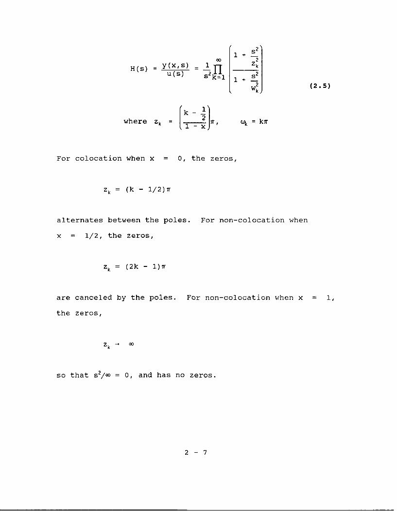
The root locus plot of Figure 2.5 contains the poles of

the solution to the characteristic equation of Eqn 2.12 as

gain k increases. The plot reveals one of the rigid body

poles (there are two at the origin) are destabilized

immediately while the flexible poles are marginally stable on

the imaginary axis.

2 - 14

ROOT LOCUS

2

1.5

u, 0.5

-0.5

-1

-1.5

-5 -4 -3 -2 -1 0 1 2 3 4 5

REAL AXIS

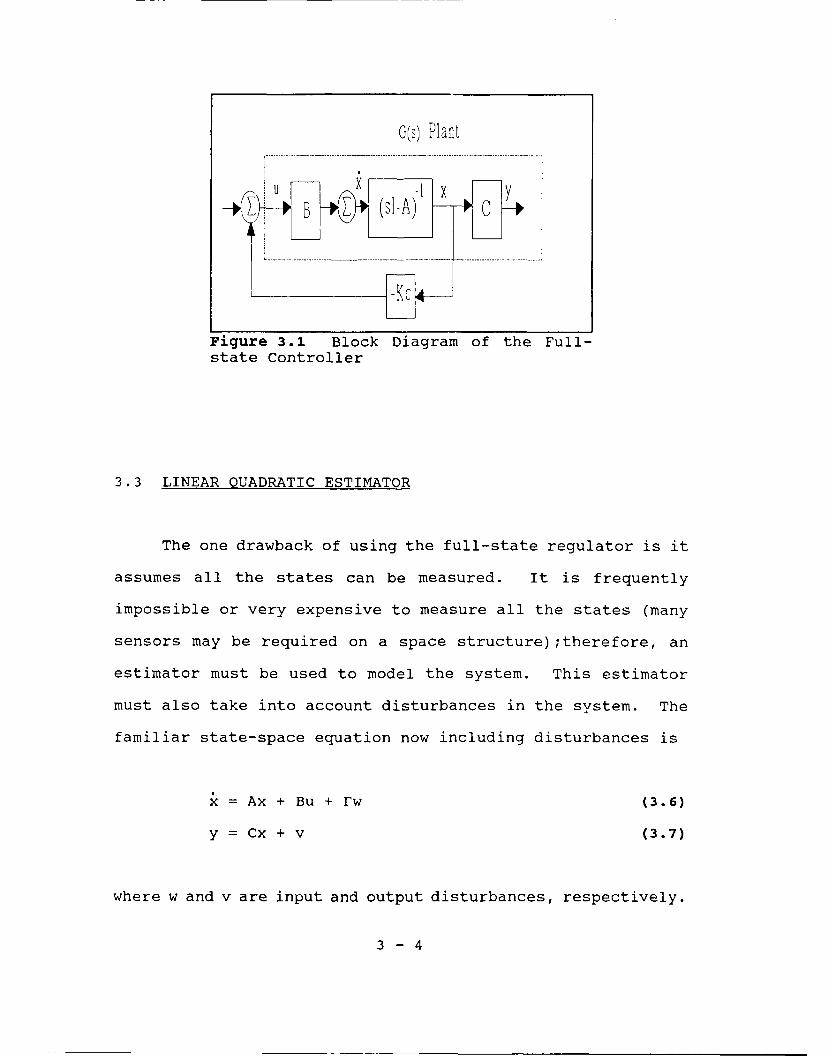
Figure 2.5 Colocation of Sensors and Actuators

The system is clearly unstable for proportional compensation.

But, a simple lead compensator can stabilize the plant as

shown in Figure 2.6.

2 - 15

ROOT LOCUS

6

4

2 2

0

-2

-4

-6-25 -20 -15 -10 -5 0

REAL AXIS

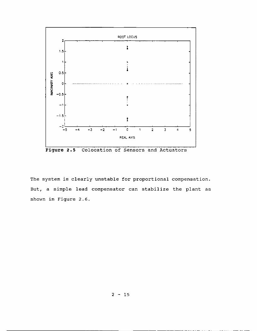
Figure 2.6 Colocation with Lead Compensation

The compensator used is the following:

GCL =-32( s + 8 ) (2.11)

As depicted in Figure 2.6, the colocated system remains stable

even under high gain feedback. The gain value was increased

from .5 to 20.

2 - 16

2.3.2 NON-COLOCATION

For the case where the sensor is located in the middle

(Y2 = 02), there is an excess pole which causes the root locus

plot to go unstable during proportional feedback as shown in

Figure 2.7.

ROOT LOCUS2.5

2

1.5

1

0.5

S-0.5

-1

-1.5

-2.5-2 -1.5 -1 -0.5 0 0.5 1 1.5 2

REAL AXIS

Figure 2.7 Non-colocation Under ProportionalFeedback with the Sensor Located at Mass J2

Partial-fraction expansion reveals this non-colocated

system does not all have the same sign for its residues, so,

the system does not have alternating poles and zeros. This is

clear by examining the poles and zeros in Table 2.1. In fact,

2 - 17

this system has the iindesirable property of being unobservable

because the zeros cancel one of the poles. For the third case

where the sensor and the actuator are located on opposite ends

of the structure, there are no zeros. Therefore the system is

clearly unstable during proportional feedback as shown in

Figure 2.7.

) 'TOCUS2

0 0.5

-0.5

-1,5

-1.5 -1 -0.5 0 0.5 1.5

REAL AX;S

Figure 2.8 Non-colocated Case Under i7-oportionalFeedback with Sensor at the Opposite End at Mass J3

Using a simple lead compensator as in the colocated case,

the first flexible pole is immediately destabilized as shown

in the root locus plot in Figure '.8. The transfer function

for the lead compensator used is

2 - 18

GcL 3 s__.2

In the n'>i-colocated case, a lead compensator is ineffective.

To ach'.;-ve stability, a higher order compensator is clearly

needed. For this thesis, the Linaar Quadratic Gaussian (LQG)

desig:, techniques will be used to design the controller.

ROOT LOCUS

...........................................................

(A 0.5

-05-

-1 -0.8 -0.5 -0.4 -0.2 0 0.2 0.4 0. 0.5

PEA1. Axis

Figure 2.9 Non-colocation With a Lead Compensator

2 - 19

III. LINEAR QUADRATIC GAUSSIAN / LOOP TRANSFER RECOVERY

3.1 LQG/LTR THEORY

Linear Quadratic Gaussian/Loop Transfer Recovery

(LQG/LTR) theory is used to design the controllers to increase

the performance and robustness of the control systems

presented in this thesis. The first step to the LQG/LTR

method is to design the Linear Quadratic Gaussian (LQG)

controller. A quadratic performance index is used to define

the LQG controller; therefore, it produces an optimal control

design stabilizes the closed loop system for the given design

conditions. The LQG controller is comprised of the Linear

Quadratic Regulator (LQR) and the Linear Quadratic Estimator

(LQE). The LQR is a full-state feedback controller and the

LQE is an estimator, commonly called the Kalman filter.

The LQG/LTR design method modifies the standard LQE and

recovers the guaranteed robustness of the full-state

regulator. This results in a closed loop system (the combined

plant and the compensator) that is robust to uncertainties,

disturbances and gain increases. The LQG/LTR methodology is

also ideal for mu?.ti-input-multi-output (MIMO) systems. The

following section will first introduce the basics of the full-

state feedback control theory. Then, the estimator and the

3 - 1

LQG controller will be presented. Finally, loop transfer

recovery is developed. These sections briefly introduce the

optimal control theory which is presented in more detail in

many other references. In particular the technical report,

Introduction to Robust Multivariable Control, by Ridqely and

Banda is extensively used by the author to develop the next

four sections [10].

3.2 LINEAR QUADRATIC REGULATOR

The linear quadratic regulator as taken from chapter 6 of

Ridgely and Banda is the following. The LQR relies on

minimizing the quadratic performance index

j = f [XI( t) Qc)x(t) + uT(t) Rcu(t) ] dt (3.1)

for the state-space Eqn 2.9.

The weighting matrices Qc and RC are chosen by the

designer depending on the importance of the state or the

control vectors. If the (A, B] pair is stabilizable, then the

optimal control law is

u = -KCx (3.2)

3 - 2

The gain matrix, K., is given by

Kc = KC-IB TP (3.3)

where P is the symmetric positive semi-definite matrix

solution to the algebraic Riccati equation

0 = ATp + PA -PBRlCBTp + Q (3.4)

where selecting Qc = Q > 0 (postive semi-definite) is a

sufficient condition for asymptotic stability of the closed-

loop system. Rc must be postive definite. Substituting the

control law, Eqn 3.2, into Eqn 2.9 yields the closed loop

system.

x= Ax + B[-Kcx]

= [A - BKC]x (3.5)

Figure 3.1 depicts the state space system of Eqn 3.5.

3 - 3

G(s) Plant

Uo

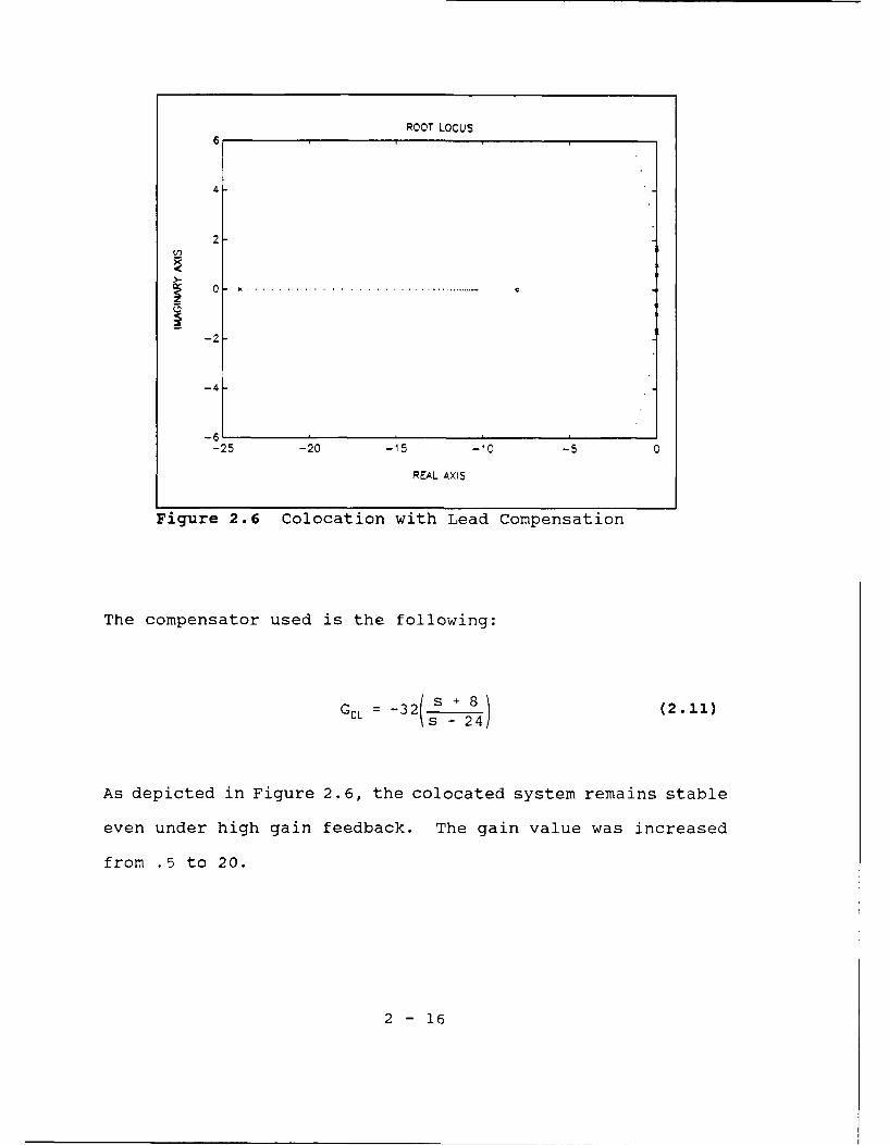
Figure 3.1 Block Diagram of the Full-state Controller

3.3 LINEAR QUADRATIC ESTIMATOR

The one drawback of using the full-state regulator is it

assumes all the states can be measured. It is frequently

impossible or very expensive to measure all the states (many

sensors may be required on a space structure) ;therefore, an

estimator must be used to model the system. This estimator

must also take into account disturbances in the system. The

familiar state-space equation now including disturbances is

x = Ax + Bu + rw (3.6)

y = Cx + v (3.7)

where w and v are input and output disturbances, respectively.

3 - 4

The disturbances are assumed zero-mean Gaussian stochastic

processes which are uncorrelated in time and have the

covariances

E[ w(t)wT(7) ] = Q 06(t-T) 0,

E[ v(t)vT(7) ] = Rf6(t-r) > 0

The covariance matrix Q0 is positive semi-definite;whereas, Rf

is positive definite. The correlation between w and v will be

assumed to be zero

E[ w(t)vT(t) j = 0

Equation 3.6 and the Kalman filter are represented by the

block diagram below.

B

T

Figure 3.2 Block Diagram of the KalmanFilter

3 - 5

The equation for the estimator is given by

Xe = Axe + Bu + Kf(y - CXe) (3.8)

where xe is the estimate of the states.

The following development of the Kalman filter is taken

directly from Ridgely and Banda. First, an assumption must be

made: the input and output disturbances, w and v, are time-

invariant and wide-sense stationary. Then the matrices Q0 and

Rf are constant. This is a valid assumption as long as the

observation of the output is much greater than the dominant

time constants of the system. The Kalman filter gain matrix,

Kf, minimizing the mean-square error

E[eTe] (3.9)

where

e = x - xe (3.10)

is

Kf = ZCTRf " (3.11)

Z, the variance of the error function, is found by solving the

algebraic variance Riccati equation

0 = AZ + ZAT - ZCTRf ICZ + Qf (3.12)

3 - 6

with Qf = rQoQT . Frequently, F = I (meaning each state has its

own distinct process noise).

The algebraic variance Riccati equation shown in Eqn 3.12

has several solutions, for which the correct solution is

unique and positive definite. A sufficient condition for Z to

exist is that the pair [A, C] be completely observable. This

condition may be relaxed to detectability, in which case it is

necessary and sufficient and Z may be positive semidefinite.

Given that Z exists, the error dynamics of the filter are

=X - e (3.13)= [Ax + Bu + rw] - [Axe + Bu +Kf{y - CXe}]

= [A - KfC]e + [F -Kf][w v]'

Therefore, the poles of [A - KfC] are the poles of the

estimator error response. The poles must be asymptotically

stable( the error must be getting smaller) if and only if the

pair [A, F] is stabilizable.

3.4 LINEAR QUADRATIC GAUSSIAN

Combining the results of LQR and LQE gives the following

expression for the LQG compensator

3 - 7

xe(t) = Ax(t) - BKcXe(t) + Kf[y(t) - CXe(t)] (3.14)

= (A - BK c + KfC)Xe(t) + Kfy(t)

Taking the Laplace transform yields the following

Xe(S) = [sI - A + BK c + KfC]- Kfy(s) (3.15)

Now, substituting this into the control law (dropping the

s notation)

u = -KcX e (3.16)

yields the expression for the LQG compensator

u = -Kc[sI - A + BK c + KfC]IKfy (3.17)

substituting the plant transfer function without the noises,

w and v,

y = C(sI - A) 'Bu (3.18)

gives

u = -Kc[sI - A + BKc + KfC] 'KfC(sI - A)-Bu (3.19)

The following figure represents the Eqn 3.19 for the LQG

compensator and the plant.

3 - 8

K's)__Compsar

Figure 3.3. Block diagram of the LQG system.

The poles of the LQG compensator are seen to be solutions of

detfsI -A + BK- + KfCE = 0

Although the poles of the regulator, the estimator and the

closed loop system are all stable, the LQG compensator poles

are not always stable. The eigenvalues of the closed-loop

system are evaluated to prove the stability. Taking the two

equations we have for the state

X = Ax + B[-KcXe] + Tw (3.20a)

Xe = (A - BK C + KfC)X e + KfCX + Kfv (3.20b)

3 - 9

Remembering that

= X - Xe (3.13)

We can put Eqn 3.20a and Eqn 3.20b into its state space form

[xA - BKA BK [ ] (3.21)= 0 A - BKf Cj~e ] r -E

Using Schur's formula, the above equation can be broken into

its determinant form

det[sI - A + BKc].det[sI - A + KfC] = 0 (3.22)

Eqn 3.22 shows that the LQG compensator is composed of the

regulator and the estimator poles which are stable.

Therefore, the closed loop LQG systems are always stable,

although the compensator itself may not be stable. An example

of this unstable compensator will be shown in the next

section.

3.5 LOG DESIGN ON THREE ELEMENT MODEL

The Linear Quadratic Gaussian (LQG) design technique

developed in section 3.4 will be used to develop a sixth order

3 - 10

compensator (same order as the plant) for both the colocated

and non-colocated cases. To make a fair design comparison,

the closed loop bandwidths for the two systems were made

equal. This bandwidth was pushed as close as possible to the

lowest frequency zero. This ensures the flexible poles will

have an effect the plant and the controller.

Briefly, the LQ Regulator is designed for the highest

bandwidth it can achieve by varying the state space weighting

matrix, QC" The bandwidth achievable is limited by the first

imaginary zero which causes the closed loop gain to go below

the -3 dB line quickly. Then, the LQ Estimator is calculated

by estimating the noise matrices, Q0 and Rf. This thesis uses

an approximate noise intensity for Q0 as ten percent of the

input force. The regulator and the estimator are then

combined to construct the LQG controller. In each case, the

design is iterated by varying the QC weighting matrix for the

LQR until they have approximately the same bandwidth. See

Figure 3.4.

3 - 11

BODE PLOT30. . . .. . . . . . . .

20

10

0

1; -10

-20\

-30\

-40- KEY

-50 non-olocoted

-6010-2 10-1 100 101 102

FREQ (Rad/Sec)

Figure 3.4 Closed Loop Bandwidths for the ThreeElement Model

The procedure leading to the LQG design was facilitated

by using a MATLAB script file, LQGD.M (See Appendix C for the

program). The weighting matrices used for the LQR for the

colocated case is

QC = diag(10 10 10' 10' 10' 10')

and for the non-colocated case is

Qc = diag(10 10 10 10 102.5 102.5)

For both cases, the noise intensity at the input for the LQE

is chosen as

Q0 = 102.

3 - 12

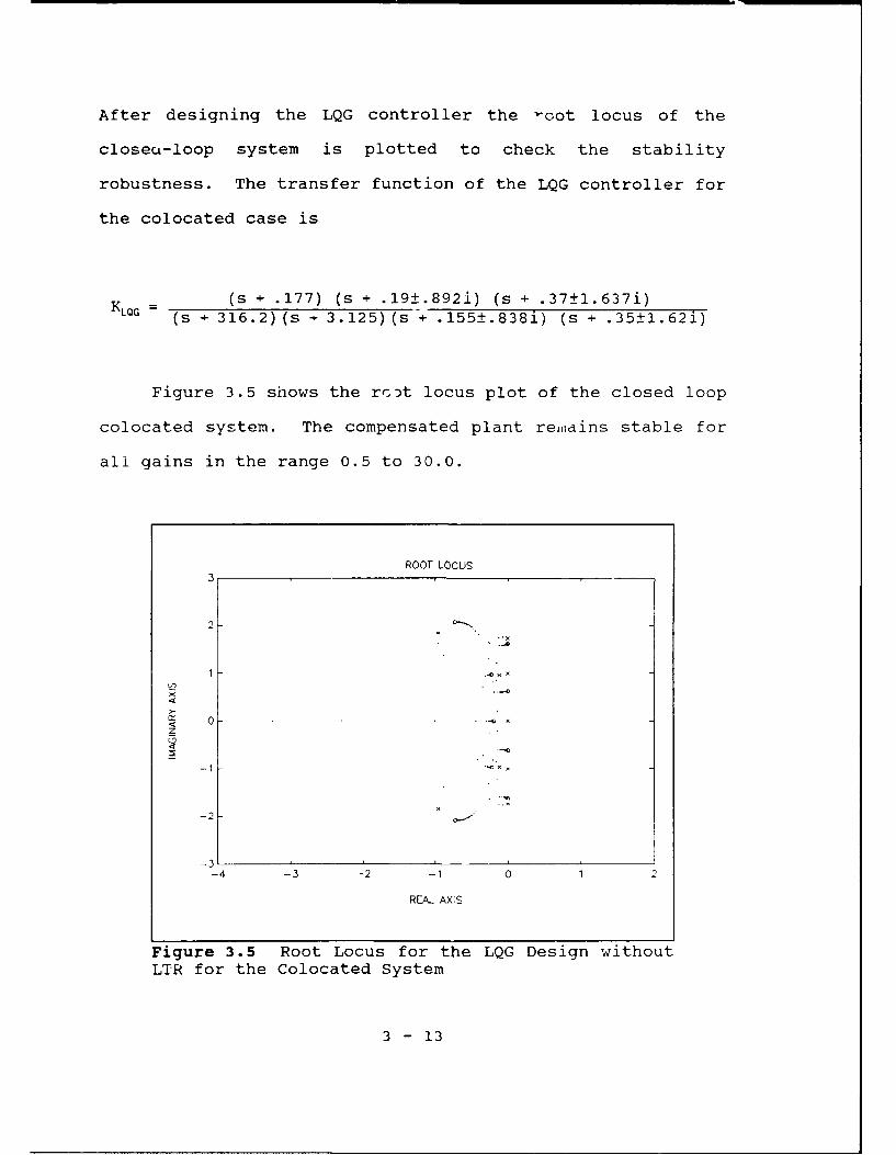
After designing the LQG controller the -oot locus of the

closea-loop system is plotted to check the stability

robustness. The transfer function of the LQG controller for

the colocated case is

KLOG = (s + .177) (s + .19±.892i) (s + .37±1.637i)(s + 316.2) (s + 3.125) (s + .155±.838i) (s + .35±1.62i)

Figure 3.5 shows the rc3t locus plot of the closed loop

colocated system. The compensated plant rewains stable for

all gains in the range 0.5 to 30.0.

ROOT LOCUS3

2

( 0 -z

-2 -.

-4 -3 -2 -2

REAL AXIS

Figure 3.5 Root Locus for the LQG Design withoutLTR for the Colocated System

3 - 13

The transfer function of the LQG controller for the non-

colocated case is

KLOG " (s + .12) (s + 1.72) (s - 7.5) (s - .208±1.07i)(s + 1.304) (s + 3.1) (s 1. 33±1.56i) (s + .952±2.li)

Figure 3.6 shows the root locus of the non-colocated

closed loop system. With increasing gain, the closed loop

poles of the compensator and the plant move into the right

half plane after a gain of k=1.75. This is a seventy-five

percent gain increase from the nominal design, but it is not

as robust as the colocated system which remains stable for

gains up to k = 30. One can see that LQG does not guarantee

stability in the face of uncertainties. In fact, for the non-

colocated system, it goes unstable rather easily. In other

words, the controller is not robust and LTR techniques are

needed.

3 - 14

ROOT LOCUS3

xx

-2-

xx

-1

-4 -3 -2 -1G 2

REAL AXIS

Figure 3.6 Root Locus for the LQG Design without LTR forthe Non-colocated System

3 - 15

3.6 LOOP TRANSFER RECOVERY

As mentioned in section 3.5, the disadvantage of the LQG

compensator is that it is generally not robust. The three

element non-colocated example went unstable after a small gain

increase. One reason is that the estimator inserted into the

LQG loop no longer guarantees the stability margins from the

full-state feedback regulator. Loop recovery technique must

be used by adjusting the Kalman filter gains.

In looking at Figure 3.3 of the LQG block diagram, the

return ratio (the characteristic equation of the SISO transfer

function) at point marked 1 determines the robustness and

performance properties for the plant, G(s). The return ratio

at point 1 is

K(s)G(s) = -Kc[sI - A + BKC + KfC]'KfC(sI - A) IB (3.23)

If you break the loop at point 1, the return ratio at point 2

is the full state feedback controller

KLQR(S) = Kc(sI - A)_1B (3.24)

The reason is when you break the loop at point 1, the signal

to the Kalman filter matrix Kf is zero. This assumes that the

A, B, and C matrices of the filter match those of the plant

exactly. Thus, the gist of the LTR theory is to make the

3 - 16

return ratios at points 1 and 2 to be the same. The following

is taken from Maciejowski (6:232].

Let * = (sI - A) and rewrite Eqn 3.23 without the

frequency domain notation (s) for brevity.

K(s)G(s) = -Kc[t + BK c + KfC]-KfC-B (3.25)

Without going into the formal proof which is shown in

Ridgely and Banda [10:ch. 8] and Maciejowski [6:232-234], one

can see how Eqn 3.25 becomes 3.24 by observing what happens as

Kf is increased toward infinity. At low frequenies (s = jw),

the term inside the bracket, t + BKc, becomes much smaller

than KfC. Thus, the bracketed term approaches [KfC] I . This

leads to

K(s)G(s) = -Kc [ KfC]1 KfC t-1 B (3.26)

K(s)G(s) = -K c I V1B

K(s)G(s) = -KcVIB

Intuitively, Eqn 3.26 shows that at low frequencies and

high estimator gains the LQG controller and the plant

approaches the behavior of a full state regulator. In terms

of poles and zeros, the effect of increasing the gain Kf

causes the closed loop poles of the Kalman filter to notch out

the plant zeros. The plant poles then move toward the

3 - 17

compensator zeros. In turn, these compensator zeros approach

the closed loop pole locations of the full-state regulator and

thus achieves the robustness guaranteed by the LQR. One can

then increase the robustness over large a bandwidth by

increasing the gain Kf. See the LTR plots of Figure 3.7 and

Figure 3.9 in Section 3.7 for examples.

However, there is a design trade off because increasing

the filter gains also increases the system noise response.

One thing to keep in mind is that increasing the gain no

longer makes it a true Kalman filter. The noise intensity is

changing from the initial assumed Qf = Q0. See the equation

below when the loop transfer recovery is applied at the plant

input.

Qf = Q, + q 2BVBT

Rf = Ro

V is any postive definite symmetric matrix and is usually

taken as identity. Q0 and Ro are the actual noise intensities.

The second term with q2 is the additional fictitious output

noise associated with LTR. When q = 0, it becomes the

standard Kalman filter.

3 - 18

3.6.1 ROOT MEAN SQUARE RESPONSE

The effect of the incredsing the fictitious noise on the

system can be measured by the Root Mean Square (RMS) response

for the LQG/LTR closed loop system. The covariance of the

output must be found by first solving the Lyapuno,, equation

for the state variance [5:104].

AQ x + QXAT + BVBT = 0 (3.27)

where

Qx E(xxT)

V= I

A and B are from state space equation

The output covariance is then

Qy = E(yyT)

which after combining with Eqn 3.27 becomes

Qy = CQxCT (3.28)

The RMS response is found by simply taking the square root of

the diagonal of the covariance in Eqn 3.28.

3 - 19

3.6.2 LTR WITH NON-MINIMUM PHASE SYSTEMS

LTR theory is not guaranteed to work with non-minimum

phase systems. Maciejowski states that some of the Kalman

filter's eigenvalues or poles from the LQG design moves toward

the plant's zeros [6:231]. This implies LTR can only be used

for minimum phase plants since the eigenvalues of the closed-

loop regulator and the estimator cannot be in the left half

plane. However, LTR may still work if the right half plane

zeros are above the cross-over frequency.

3.7 LOOP TRANSFER RECOVERY ON THE THREE ELEMENT MODEL

For the three element model, the colocated system shows

excellent loop recovery properties throughout its frequency

range (10-2 to 102 rad/sec). Examination of the system

eigenvalues shows that the poles of the plant and the

compensator moving toward the poles of the full-state

controller. Figure 3.7 shows clearly the open loop system

approaching the target loop of the full-state. The high

fictitious noise of 1015 was able to get full recovery (as

evident by the loop matching the full state). The root locus

of the closed loop K(s)G(s) system shows it retains excellent

robustness with the poles going unstable after a gain increase

of k = 28.5 at q2 = 1015. This is almost a three-thousand

3 - 20

percent gain variation that the colocated system can handle!

See Figure 3.8 for the root locus plot.

The non-colocated system does improve its robustness

slightly with LTR, although loop recovery is not as easy to

achieve with the non-colocated system (indication that this

type of system is non minimum phase). See Figure 3.9 for

q2 = [ 0 1018 o1020 . Notice the good recovery at low

frequencies, but not at high frequencies. In fact there are

small spikes in the loops where it diverges from the full

state's open loop. Using a large fictitious noise value of

1020 did get good recovery and damped out the spike. It also

improved the robustness of the system to gain variations up to

k = 4. See Table 3.1

Table 3.1 LTR for Colocated and Non-colocated Three ElementModel

2 colocated non-colocated

0 30 1.7510 30 1.7510 17.0 1. 25

109 6.5 1.501012 8.0 1.501015 28.5 2.01018 30 2.751020 30 4.01024 30 7.0

The table shows a decrease in the colocated system when

q2 = 19 and 1012. Starting at these fictitious noise values,

3 - 21

the colocated RMS response becomes greater. Then the RMS

response stabilizes after q2 = 1015. See Table A.l in Appendix

A. Thus, the increase in the noise of the colocated system

appears to have an effect on the robustness of the system to

loop transfer recovery.

In looking at the LTR plots and the Bode plots, the non-

colocated system has the advantage of having the high

frequency roll-off. This is desirable to prevent the noise

from amplifying and driving the system unstable. The non-

colocated system does have a major drawback in that it behaves

like a non-minimum phase system with RHP zeros. Figure 3.10

shows the root locus plot using the fictitious noise value of

1018. Note the poles moving into the right half plane as if

there were RHP transmission zeros.

3 - 22

LOG .1th LTR140 !U.t r' P

8000

400

20 2000

-200O

-400 0

-- 00-1 0 - 00 1-600 -4000 -200 0 1 200

RRCIEALY AXIS.

Fiue3LRfor the Colocated System

ROO LOC23

LQG .1th LTR

1220

q401

202

-0 q!l

10-2 10-' 100 10' 10'

FREOUENCY ( Rod/Sec

Figure 3.9 LTR for the Non-colocated System

ROOT LOCUS

30-

20

10-

-20-

-30

-35 -30 -25 -20 -15 -10 -5 0 5 10 15

REAL AXIS

Figure 3.10 Root locus for the LQG desing withoutLTR for the non-colocated system

3 - 24

3.8 STEP RESPONSE

The unit step input will now be applied to the closed

loop full state regulator. The unit step input response is

useful for analyzing the performance characteristics of a

system. The time response is useful in revealing the rise

time, settling time, and the steady state value [9:40].

The RHP zero has an interesting influence on the step

response. Reid states that for non-minimum phase systems the

initial response is negative. This means the system moves in

the opposite direction in relation to the final steady-state

value. If the system has no zeros (i.e. the non-colocated

three element mass model), the initial response will be flat.

The plot of the step response for the colocated and non-

colocated systems are shown in Figure 3.11. The non-colocated

system shows a flat response initially since it has no zeros.

The colocated step response shows it fluctuates as it comes to

its steady-state value. This is the result of the imaginary

zeros and because the poles are lightly damped.

3 - 25

STEP RESPONSE1.2

0.2

0.2 //

// KEY./ colocoted " -

... ----- non-colocoted

-0.2 10 2 4 6 8 10 12 14 16

TIME (sec)

Figure 3.11. Step Response of the Three ElementModel

3.9 CONCLUSION

The colocated LQG/LTR system is very robust to gain

variations. However, the robustness decreases for q2 = 109

through 1012. The RMS response at these fictitious noise

values show that the colocated system is much higher than the

non-colocated system. While the non-colocated case has low

RMS response, it is not robust in comparison to the colocated

system. It does improve slightly for very large q2 values.

See Table A.I in Appendix A. Looking at the closed loop

bandwidths show that the non-colocated system has very good

damping and has the desirable high frequency roll off. The

colocated system has little damping of its flexible poles. In

this regard the non-colocated case is better.

3 - 26

The step response to the unit input also shows the non-

colocated system has better damped poles and a smoother rise

time curve. However, the system exhibits non-minimum phase

behavior of having no initial response to the input for the

first two seconds. See Figure 3.11. This maj be an

unacceptable response. Recall this single motion DOF model

did not have RHP zeros to cause a negative response typical of

non-minimum phase systems. This leads to the next chapter

which shows that non-colocated systems have RHP zeros for two-

motion DOF models.

Observing the closed loop eigenvalues of the LQG/LTR

controller showed how it becomes robust. LQG design is helped

by LTR because as the fictitious noise is increased, the

compensator poles move toward the open loop planK zeros to

notch them out. The Kalman filter accomplishes this task

since its closed loop poles (A - KfC) at high q2 values moves

right onto the plant zeros. On the other hand, the

compensator zeros move toward the stable poles of the closed

loop regulator (A-EKC). Thus, the plant poles during

compensated feedback must move toward the compensator zeros

which guarantees the stability and the robustness of the

closed loop full-state regulator. In essence, the LQG

compensator inverts the nominal plant and substitutes the

desired LQR dynamics.

To summarize for the three element model using an initial

noise intensity of Q0 = 102, the colocated system can be made

3 - 27

robust by just using the LQG compensator; whereas, the non-

colocated system can be improved slightly with LTR. To get

better rise time curve and damping for the colocated system

requires a lower bandwidth away from its low frequency

imaginary zeros and therefore a drop in performance. On the

other hand, the non-colocated system can achieve a higher

bandwidth and better damping since it has no imaginary zeros

affecting the crossover frequency it can attain.

3 - 28

IV. A TWO MOTION DEGREE OF FREEDOM SYSTEM

4.1 Introduction

The first example presented in this thesis of the three

element lumped mass system showed the non-colocated system was

technically minimum phase (i.e. no zeros in the right half

plane). However, the system showed non-minimum phase

characteristics. For instance, the step response had initial

flat resronse characteristic of a non-minimum phase system

with no zeros. Loop transfer recovery to the full-state loop

shape was limited, especially in comparison to the colocated

loop recovery shapes. At high frequencies, it exhibited the

characteristic steep roll-off of a non-minimum phase system.

4.2 EXACT SOLUTION OF A TRANSVERSE BEAM

The three element lumped mass model is a single motion

DOF system since it only has plane rotation about one axis.

The numerator of the non-colocated transfer function was

zeroth order and had no roots (refer to section 2.3.2). Thus,

a single motion DOF system will not yield any zeros in the

RHP. Therefore, a two motion DOF system will be examined to

4 - I

demonstrate the non-minimum phase behavior for non-colocated

structures. A two-dimensional beam which can translate and

rotate will be needed. As shown in Reference 14 by Bryson and

Wie, a Bernoulli-Euler beam with transverse bending vibrations

will have zeros in the RHP [14:165].

7

El, L,E(

Figure 4.1 Free-free Transverse Beam

The equation of motion for the transverse beam is

y(IV, (x, t) + (x, t) = 0

(4.1)

where y(IV) a a Y and a y(x4 at 2

and y(x,t) is the transverse displacement.

The displacement variables x and y are in units of L,

time in units of (cL4/EI) /2. a is the mass density per unit

length. Taking the Laplace transforms of Eqn 4.1 yields

4 - 2

y(iV) (x,s) + s2 y(x,s) = 0 (4.2)

Thus the transcendental transfer functions for free-free

boundary conditions for the two cases of colocation and non-

colocation yields the following

v(0,s) = sinhXcosX - coshlsinX (4.3a)u(s) A3 ( 1 - coslcoshA )

y(ls) = sinhA - sinX (4.3b)u(s) A3 ( 1 - coslcoshA )

where ;,= - s2 or s = jw (in the frequency domain)

Solving for Eqn 4.3a directly shows the poles and zeros

alternating on the imaginary axis of the complex plane as

shown in 1igure 4.2. The non-colocated case, Eqn 4.3b, has

infinite number of reflexive zeros on the real axis as shown

in Figure 4.3.

4 - 3

120.90A

61.67C49.96

22.37x15.41

Figure 4.2 Exact Poles/Zeros of aColocated System

Figure 4.3 Exact Poles/Zeros of aNon-colocated System

4 -4

4.2.1 MODAL TRUNCATION AND ITS EFFECT ON ZERO LOCATION

Eqn 4.3 for the closed form solution to the Bernoulli-

Euler beam shows that non-colocated structures have RHP zeros

on the real axis. When the model is truncated, the finite

dimensional form of the transfer function derived from Eqn 2.1

shows that there can be complex zeros as well.

y(l,s) , 2 I 4 (-l)i!+a(- + E (4.2)U(S) S2 S= s2 +

Reference 14 shows that Eqn 4.4 yields zeros on the real axis

of the RHP when N = 1. When N = 2, Eqn 4.4 yields complex

zeros in the RHP. Thus, a truncated model will not

necessarily have all its zeros on the real axis. But, it will

have RHP zeros.

4.3 APPROXIMATE SOLUTION BY FINITE ELEMENT METHOD

Using partial differential equation representation for

structures can be difficult to solve; therefore, the Finite

Element Method (FLM), will be used to analyze a two motion DOF

beam. The author used the FEM computer program, ANSYS, to

solve for the eigenvectors and the eigenvalues needed to get

4 - 5

the equations of motion (EOM).

Using the finite element approach as presented by

Meirovitch [8:ch.4], the general EOM for an undamped system is

[m](q(t)) + [k](q(t)) = (Q(t)) (4.5)

where [M] and [K] are constant mass and stiffness

matrices of size n (number of modes used)

(q) and (Q(t)) are the column matrices of

generalized coordinates and generalized forces,

respectively.

Eqn 4.4 is difficult to solve because of the coupling in

the mass and the stiffness matrices. To solve these linear

2nd order equations, the linear transformation

(q(t)) = [u](r(t)} (4.6)

where (r(t)} is a new set of generalized coordinates,

[u] is a transformation matrix or a modal matrixcomprised of the eigenvectors,

is used to decouple the mass and stiffness matrices so that

they are diagonalized. The EOM using the new generalized

coordinates is

[m][u] ( (t)) + [k][u](?7(t)} = (Q(t)} (4.7)

4 - 6

Pre-multiplying by [u]T results in the modal EOM

[M]{(r(t)) + [K](n(t)) = (N(t)} (4.8)

where [M] = [u]T[m][u] is the modal mass matrix,

[K] = [u]T[k][u] is the modal stiffness matrix.

Orthogonality of the modal matrices diagonalize the mass

and the stiffness matrices (given that they are constant and

symmetric). It is common to normalize the mass matrix to an

identity matrix. Multiplying by the inverse of the identity

mass matrix makes the stiffness matrix equal to the

eigenvalues since w 2 = K/M. The final form of the EOM is then

[I] {u(t) ) + [2] (77(t) ) = {N(t) ) (4.9)

This form of the EOM is readily available from finite element

computer programs such as ANSYS. Eqn 4.8 can be put into the

state-space form of Eqn 2.8

= [ 2 ] + UT (4.10)

where u is the input control force,

4 - 7

Linear transformation must also be applied to y = Cx to get

the output matrix in the state space equation form.

y = .[u] [7 ]'T (4.11)

Thus, the state space equation for output becomes

y = [ C[u] : 0 ]x

The matrix C is padded with zeros to match the size of the

state vector x (since no velocity measurements are taken).

The C matrix in Eqn 4.11 for a single output case will be a

row matrix of size 1 x n with ones at the nodes of interest.

4.4 TEN ELEMENT TRANSVERSE BEAM EXAMPLE

To show that the FEM can produce the [A], [B], and [C]

matrices required for the state-space equations, a ten element

transverse beam is modelled in ANSYS. See Appendix B for the

ANSYS data input file.

4 - 8

y X

x F

node 1 rode 1

Figure 4.4 Ten Element Transverse Beam

The two dimensional beam element (STIF 3) is an uniaxial

element with tension-compression and bending capabilities. It

has three DOF at each node: translation in the x and y

direction; and rotation about the z axis.

Uyl Uy2

I &x 2

STIF e1enznt

Figure 4.5 DOF for the TwoDimensional Element

For this example problem because bending is the primary

mode of interest, x translational DOFs were neglected. The

ten element beam has a total of 40 DOF (4 DOF/element x 10

elements). Eliminating the DOFs at the internal nodes due to

the constraints results in total of 22 unkown DOF. Solving

this free-free beam using modal analysis in ANSYS produces a

4 - 9

22x22 modal matrix, [u], assoicated with the DOF

Uyl

Oz1

DOF = 1 !

uy11Ozl

The A matrix is formed from the mass and stiffness matrices,

but ANSYS has normalized the mass matrix to identity so that

A can be derived by Eqn 4.9. The A matrix is

r 0 22x22 I22x221A =

[_W [ 2 2

x2 2

0 22X22

ANSYS outputs the eigenvalues in natural frequencies in units

of cycles per time and must be converted to radians per time

before using in the A matrix. Listed in Table 4.1 are the

eigenvalues from Ansys compared to the closed form solution

for free-free transverse beams [14:275].

Table 4.1 Eiqenvalues from Ansys and the Closed Form Solution

Ansys Closed Form Solution Error

0.0 Hertz 0.0 0.0 %0.0 0.0 0.04.072 4.088 0.411.196 11.259 0.621.884 22.080 0.9

4 - 10

Note the first two modes are the rigid body modes (X = 0.0).

The error is less than one percent for the first five modes,

which shows the accuracy of the model with the full twenty-two

modes. Later section will compare the eigenvalue solution for

just four modes. The Q force matrix is

00

Q= 0

1

where 1 has been placed at the 21st row representing node 11

in the y direction. Therefore the B matrix is

[0

where UTQ is the 21st row of the transposed modal matrix.

The output matrix is

4 0 00.10]

4 - 11

where the ones represent a displacement sensor at node 1 (non-

colocated) and node 11 (colocated). Remembering

C = [c[u](2x22) o(2X22)]

where C[u] becomes the 1st row and the 21st row of the modal

matrix, [u].

4.4.1 MODEL REDUCTION TO FOUR MODES

Because of the large size of the A matrix (44x44), the

model was reduced to only the first four modes. For the ten

element beam, going from twenty-two to four modes still

produced accurate results for the first two flexible poles.

This is evident by examining Figures 4.6 and 4.7. The Bode

plot of the reduced beam with four modes is compared with the

frequency response spectrum from ANSYS (KAN 6 Analysis). In

this way, two different methods are used to find the transfer

function between input and output for a beam.

The reduction produced a 8x8 A matrix containing the mode

shapes of interest. The first four eigenvalues are still very

accurate to the closed form solution shown in Table 4.1.

4 - 12

0.0 Hertz

0. 87!e-64.23212.727

The second mode is the rigid body rotation, so the value was

made zero. The first flexible pole is accurate to within 3.5

percent of the closed form solution. See Figure 4.8 for the

mode shapes associated with the eigenvalues.

4 - 13

BODE PLOT

IC'

MATLAEB'

1 C -

51 A',SY S

me 10' 102 1C,3

FREQ (Red/Sec)

Figure 4.6 Bode Plot Comparing Frequenc,%,, Responserf 11 Modes to the Reduced 4 Modes for theColocated Beam

muDE PLOT

1 -- ,

FR[E (e i, 'S~e

Figure 4.7 Bode Plot Comparing the Frecjuernc,Response of 11 Modes to the Reduced 4 Modes for theNon-colocated Beam

4 - 14

y]

Figure 4.8 The Four Mode Shapes of the TenElement Beam

4 - 15

The final A matrix is

0 0 0 0 1 0 0 0

0 0 0 0 0 1 0 0

0 0 0 0 0 0 1 0

0 0 0 0 0 0 0 1A= 0 0 0 0 0 0 0 0

0 0 0 0 0 0 0 0

0 0 -7.06x10 2 0 0 0 0 0

0 0 0 -6.39x10 3 0 0 0 0

The B matrix is

00

0

0B=3.288

').7273.393

4.128]

The C matrix is

[ 3.288 0.727 3.393 4.128 0 0 0 0'C = [-2.272 2.485 3.654 -3.011 0 0 0 0,

The eigenvalues of the A matrix are the system poles and

the transmission zeros are found using the tzero command in

MATLAB. They are listed in Table 4.2.

4 - 16

Table 4.2 Poles and Zeros of the Ten Element Beam

Poles Colocated Zeros Non-colocated Zeros

0,0,0,0 r/s 0,0 0,0±26.59i ±18.32i ±32.52±79.97i ±61.89i ±65.20

Note the extra pair of zeros for the second rigid body motion

is canceled by the pair of zeros for the colocated and non-

colocated zeros. This pole/zero cancellation did not cause

observability problems. Shown below is the Bode plot of the

open loop plant for both the colocated and non-colocated

systems. Note the dips in the colocated plot indicating it

has imaginary zeros;whereas, the non-colocated has no dips

because its zeros are on the real axis. The non-colocated low

frequency gain is little less than the colocated

gain;therefore, a pre-filter gain of 2 is required to the

input of the B matrix to make the two systems equal for

comparison purposes.

4 - 17

I,

10'

Figure 4.9. Bode Plots of the Colocated and Non-colocated Ten Element Beam

4 - 18

4.5 LOG/LTR CONTROL DESIGN ON THE BEAM

The control design on the transverse beam produced

interesting results. The control design without LTR (the

fictitious noise parameter q = 0 ), resulted in the colocated

system being robust to large gain variations (from 0.5 to 43).

The non-colocated system did not improve with LTR as expected

of a non-minimum phase system.

Both systems were designed to have the same bandwidth of

about 8 rad/sec. Figure 4.10 represents the Bode plot of the

closed loop bandwidths for both cases. The weighting matrices

used for the LQR for the colocated case is

Qc = diag(105 1 0 5 1 0 5 1 0 5 1 0 1 0 103 L03),

and for the non-colocated case is

Qc = diag(104-5 104.1 104 104 103 103 103 103)

For both cases, the noise intensity at the input for the LQE

was selected as

Q4 = 101

4 - 19

BODE PLOT60

40

20

C3 0

S-20

-40

-0 - c :o- c oted - - -

10' 102 10,3

Figure 4.10 Closed Loop Bandwidths for the TenElement Beam

The root locus plots show the poles of the closed loop

system as gain is varied. The colocated system went unstable

at gain of k = 43. See Figure 4.11. This system became less

robust after LTR for q2 = 109" Then the system started to

increase in robustness until the gain value exceeded 100.

Observing the LTR plots of Figure 4.13 clearly shows that the

system gained the robustness of a full-state regulator. See

Table A.2 in Appendix A for the results from the design

iterations. Figures 4.14 shows the root locus plot for

q2 = 1012. Note the highest frequency pole is the one that

goes unstable. So, this system is very robust for the lower

frequency poles.

4 - 20

The non-colocated case was not able to get full loop

recovery no matter how much fictitious noise was added. In

fact, gains after q = 1012 made no improvement on the low

frequency recovery. See Figure 4.15 for the LTR plots. The

poles became unstable after a gain of k = 2 for all q2 values.

See Table A.2 in Appendix A. The root locus plot for q2 = 1012

is shown in Figure 4.16. This plot clearly shows the poles

moving toward the right half plane zeros.

POOT LOCUS80 .

..........................

S20

0 ,,..

-40 "

x

-0 -25 -20 -15 -10 -5 0

REAL AXIS

Figure 4.11 Root Locus for the LQG Design Without LTR forthe Colocated System

4 - 21

ROOT LOCUS

80

60-

40

_ 20 o

- -a0

-40 "

-60-

-80 __ __ _ __ _ __ __ _ __ _ __ _ __ __ _ __ _ __ __ _ __ _ __ _

-60 -40 -20 0 20 40 60

REAL AYIS

Figure 4.12 Root Locus for the LQG Design Without LTR forthe Non-colocated System.

4 - 22

LQG WIth LTR

80

60

+0. 220

- 20 q1

-40

-00 -21-01 -1102 -503

FRQEALY AXIS

Fgr43LR for the Colocated System

4 - 2

LOC with LTR

10 101122 0

40

-401

-60O

-10-0 2 10 12 0 3

FRQEALY RAIS )

Fgr 45LRfor the Non-colocated System

4 - 2

4.5.2 STEP RESPONSE

The step response plot clearly shows which system is non-

minimum phase. The non-colocated system has an initial

negative response to the step input. Otherwise, this system

has much better damping than the colocated system which has

ringing.

STEP RESPONSE1.2

06

0.4

I/ KEY

/ cOIccOted

- 20 01 02 03 04 G5 06 0.7 S0 LI 1

71ME (Se':)

Figure 4.17 Step Response of the Ten Element Beam

4 - 25

4.6 CONCLUSION

For the ten element beam after large amounts of

fictitious noise was added, the colocated system became very

robust as it approached the target full-state regulator. On

the other hand, the non-colocated system did not get any

recovery for any value of fictitious noise. The RMS response

of the colocated system was also much less than the non-

colocated system. See Table A.2 in Appendix A.

The step response for both systems had similar results as

the three element lumped mass example. The colocated system

had ringing in its rise curve due to the lightly damped poles

and the influence of the zeros on the imaginary axis. The

non-colocated rise curve had the initial negative rise

associated with the RHP zero.

Reviewing the closed loop pole locations show that

LQG/LTR designs agree with theory. As q2 is increased for

the colocated system, the Kalman filter's closed loop poles

notches out the plant zeros. Meanwhile, the LQG/LTR

compensator zeros move toward the closed loop poles of the

full-state regulator. In turn, the root locus shows the

plant's poles moving toward the compensator zeros during

feedback. This is clear in Figure 4.15 of the non-colocated

system which shows the filter poles notching out the plant

zeros in the LHP. Thus, the compensated feedback system

achieves the robustness of a full-state regulator. The non-

4 - 26

colocated system can not achieve loop recovery since it has

RHP zeros which prevent the Kalman filter poles from notching

out the zeros. However, the colocated system has higher noise

which seems to cause the design trade-off in improving system

robustness with LTR.

4 - 27

V. FINITE ELEMENT MODEL OF CONTRAVES P52F GIMBALS

5.1 FINITE ELEMENT MODELING

The gimbal structure used in this investigation is a

target motion simulator built by Contraves USA. This gimbal

must be robust to parameter variations because it must

aG.omodate many different types of missiles for testing. The

control design must be able to handle the changes in the mass

and inertia of the different payloads.

The gimbal has an inner (azimuth axis) and an outer

(elevation axis) gimbal arrangement. The gimbal is driven by

hydraulic actuators that provide torque and uses position and

torque transducers (sensors) . The torque for the finite

element model is applied on a node on the inner gimbal at

point A in Figure 5.1. Point A is also the location of the

colocated sensor and Point B is the location for the non-

colocated sensor. The two gimbals are connected together by

a pipe element (STIF 12) with soft beam elements (STIF 3)

representing the bearing connection that simulates the

rotation of the inner gimbal. For this thesis, the outer

gimbal was fixed against rotation. The model is three

dimensional in that it has all six DOF (xyz translation and

rotation) associated with the nodes.

5 - 1

The ANSYS model in Figure 5.1 has over one thousand

elements. Because of the large number of modes available, the

modal analysis used only the first five modes.

Figure 5.1 Contraves P52F Gimbal

5 - 2

This truncated model produced the following eigenvalues in its

natural frequency form.

S=1.418 Hz13.73661.4603940.8614761.030

The first mode was found to be the rigid body mode of the

inner gimbal. So, this frequency was taken as zero. The mode

shape plot of Figure 5.2 shows the rotation (the solid shape)

and the dotted line representing the original shape. The

second mode caused a pole/zero cancelation and was omitted

from the analysis. The last two eigenvalues are at very high

frequencies. Thus, the only effective flexible pole is the

third mode at 61.46 Hz or 386.2 rad/sec.

Table 5.1 Poles and Zeros of the Contraves Model

Poles Colocated Zeros Non-colocated Zeros

0,0±386.2i ±173.6i ±229.7±24761.Oi ±2247.8i ±8667.1±29914.Oi ±26915.Oi 0.0 ± 11631.Oi

Note Table 5.1 shows the non-colocated case has an imaginary

zero. This is not that unusual and is the result of modal

truncation. The bode plot shows the poles and zeros in Figure

5.3.

5 - 3

Figure 5.2 The First Mode Showing the Rigid BodyRotation

5 - 4

BODE PLOT

10-'

102/ I

EY

1 D- 4

OIOC tea

103 102 103

FEEC (ReciSe:

Figure 5.3 Bode Plots of the Colocated and Non-

colocated Contraves Model

The accuracy of the truncation compared to the frequency

response of the structure shows the dominant pole at 386

rad/sec was matched very well. But, the frequency response

shows there is also another pole/zero pair near 250 rad/sec

that the truncated model does not have. See Figures 5.4 and

5.5 on the next page. Considering the fact this model has all

six DOF and our sensor is only taking the rotational

measurement, the author considers this to be an acceptable

since the closed loop bandwidth is at 100 rad/sec which is

below this first pole at 250 rad/sec. A position sensor

located elsewhere on the model may sense the pole missed by

the sensor located at points A and B in Figure 5.1. Then the

control problem becomes single input and multi-output; but,

this thesis is only examining the SISO case.

5 - 5

BODE P .CT

102 1- 14,

FRC-Pc/Sc

Fiur 5. Trnae MdlCmard t h

Frqec Resons fo th----1td as

Figure 5.4 Truncated Model Compared to theFrequency Response for the Col-ocated Case

5 -

Further investigation was done to better match the

fr-quency response curve by using a MATLAB script file ANSYS.r!

written by Professor Bradley Liebst to do a least squares fit.

This method produces a transfer function in polynomial form.

The curve fit modeled the first two flexible poles well and

produced an eighth order polynomial. See Figure 5.6.

SoId - True Trans. Fur c. I oshed - Best Fit Trans. Func.10 1 I. . .. . .

100

10-2K

Q-2

10- 3

1 0--

10-5

1 O-e I. 1.100 10' 102 103

Frequency (Hz)

Figure 5.6 8th Order Curve Fit Using Ansys.m tothe Frequency Response Data

However, converting from transfer function to state space

produced a poorly conditioned (A, B, C, D) representation. It

appears the most numerically reliable method for state space

design is using the FEM modal analysis presented in Chapter 4.

5 - 7

5.2 LOG/LTR DESIGN ON THE GIMBAL

The final A matrix after truncation and reduction is

8 x 8 in size. The state weighting selected for khe colocated

system is

QC = diag(106 106 1 03 103 102 102 10 10)

and for the non-collocated sytem is

K diag(101-5 105"5 101 1 03 10? 102 10 10)

For both cases, the noise intensity at the input was model2d

as

Qo = lG

The closed loop bandwidth for the LQG designs are shown

in Figure 5.6 where the crossover frequency is defined as -3dB

below the 0dB axis.

5 - 8

ODE PLOT

40

20

-20

-40

-60- otoccted

norl-COlocoted -- -

-80-

101 102 103 104 105 Joe

FREO (Pod/Sec)

Figure 5.7 Closed Loop Bandwidths for theContraves Model

The LQG design without LTR for the colocated case

produced a system that went unstable at gain k = 5.5. The

non-colocated system went unstable at k = 2.5. Interestingly,

the LQG design for both systems placed compensator zeros in

the RHP. It was not until the fictitious noise value became

q2 = 109 did the all the colocated compensator zeros move into

the LHP. At this time, the system became very robust and it

wpnt unstable at k = 25. The non-colocated case never gained

any robustness after LTR. Its compensator zeros remained in

the RHP for all fictitious noise values. See the results in

Table A.3 in appendix A. The loop transfer recovery plots and

5 - 9

the root locus plots for the colocated and non-colocated cases

are shown on the following pages.

5 - 10

L.C3 -t" LTP

50'-

10,J2 103 10. IC ,

PE. ,NCZ' ( Rod,'Sec

Figure 5.8 LTR for the Crn1ocated System

08G R007 !.OC1L'S

4

3-

- I-

-5 -4 - 2 -

REAL AxIS X10,

Figure 5.9 Root Locus for the LQG Design with LTRfor the Colocated System

5 -1

FP .GE-C .. " Se

Figure 5.10 LTR for the Non-colocated System

ROCT LOCUS

-2 -1 -

REAL AXIS

Figure 5.11 Root Locus for the LQG Desiqi with LTRfor thie lNcn-colocated System

5.3 STEP RESPONSE

The step response of Figure 5.12 shows the colocated and

non-colocated systems having similar rise times. Both systems

have good damping of its poles with the colocated showing a

small fluctuation due to its zero on the imaginary axis. The

non-colocated system because it has RHP zeros has the initial

negative rise in its step reponse.

K.K'

T

Figure 5.12 Step Response of the Contraves Gimbal

5 - 13

5.4 CONCLUSION

The non-colocated system since it was non-minimum phase

could not recover any robustness with LTR. On the other hand,

the colocated system after sufficient fictitious noise was

added at the plant input increased its robustness. See Table

A.3 in Appendix A.

The RMS noise responses for the colocated system was

generally larger than the non-colocated system due to the

larger QC weighting matrix used. The unit step input response

revealed the negative rise expected from non-minimum phase

systems for the non-colocated case. Both rise times were the

similar and both had good damping.

Some modeling inaccuracies were introduced by modal

truncation of the very large system to only the first five

modes. Even then, one of the modes proved to be unobservable

and had to be removed from the analysis. More analysis with

higher order models might be needed to more accurately model

the system.

5 - 14

VI. CONCLUSIONS AND RECOMMENDATIONS

6.1 SUMMARY

Chapter II introduced the three element lumped mass model

to illustrate basic principles of pole/zero patterns

associated with different cases of sensor and actuator

locations. The colocated system (sensors and actuators at the

same location) has the desirable property of alternating poles

and zeros on the imaginary axis. This pole/zero pattern makes

it easy to stabilize the system with a simple le&d

compensator. The non-colocated system could not be stabilize:

with a lead compensator. Because the three element model is

a single motion DOF system, it did not have any RHP zeros.

But, it exhibited non-minimum phase like behavior. The non-

colocated system required a higher order controller to

stabilize it.

Chapter III introduced the LQG/LTR theory used to design

the higher order controller for the non-colocated system.

Despite large fictitious noise added, loop recovery was

limited and marginally successful only at low frequencies. It

maintained its high frequency roll-off characteristic of a

non-minimum phase system.

6 - 1

To show RHP zeros of a non-minimum phase system, Chapter

IV introduced the FEM and the ten element transverse beam.

This model exhibited the RHP zeros for the non-colocated case.

As expected of a non-minimum phase system, LTR had little

effect on improving the robustness in comparison to the

colocated system. Because the LTR theory relies on placing

the poles of the Kalman filter at the plant's zeros, the RHP

zeros make this impossible to accomplish. For the colocated

system, LQG design without LTR was sufficient to make it very

robust. However, LTR made the system much more robust as it

approached the robustness of the target full-state loop.

Chapter V designed the LQG/LTR controllers for the

Contraves gimbal. The final results were similar to the ten

element beam. LTR made the colocated system more robust,

although the robustness did not increase linearly. Of course,

the non-colocated system which had RHP zeros had unsuccessful

LTR.

This finite element model was much more complex than the

beam;therefore, modal truncation did not model one of the

system's flexible poles at 250 rad/sec. However, this

flexible pole was above the design bandwidth of 100 rad/sec.

The author considered the system to be accurate enough for

design comparisons.

Interesting observations were made concerning the LQG/LTR

controllers. LQG design is helped by LTR because as the

fictitious noise is increased, the compensator poles move

6 - 2

toward the open loop plant zeros to notch them out. The

Kalman filter accomplishes this task since its closed loop

poles (A - KfC) at high q2 values moves to the plant zeros.

On the other hand, the compensator zeros move toward the

stable poles of the closed loop regulator (A-BKc). Thus,

during compensated feedback the plant poles move to the

compensator zeros which recovers the robustness of the full-

state regulator.

The two designs are compared in Table 6.1. The following

were used as criteria:

A. Robustness

1. Gain at which the root locus goes into the RHP

2. Whether full recovery to the target full state loopis achieved

3. Alternating poles and zeros indicating whether asystem can be easily stabilized

B. Performance

1. Bandwidth

2. Step response

- settling time- ringing- initial negative response or no response

3. Damping

4. RMS noise response

6 - 3

C. Designability

1. RHP compensator poles

2. High frequency roll off

3. State weighting required

Table 6.1 Comparison of Colocated and Non-colocated Systems

COLOCATED DESIGN NON-COLOCATED DESIGN

A.1: Robust to gain variations Not robust to gainvariations

A.2: LTR is possible over a LTR is not achieved,large bandwidth especially at high

frequency

A.3: Has alternating poles/zeros No alternating pattern

B.1: Lower bandwidth achievable Higher bandwidth achievable

B.2: - Faster settling time - Slower settling time- Ringing - No ringing- n/a - Initial negative response

B.3: Poorly damped poles Poles damped well

B.4: Higher RMS response Lower RMS response

C.I: Compensator can have RHP poles for both systems

C.2: No high frequency roll-off High frequency roll-off

C.3: Larger state weighting Smaller state weightingmatrix required to matchbandwidth

6 - 4

6.2 CONTRIBUTION

It appears each system has its own advantage. The

colocated system is very robust and can handle large gain

variations. But, the colocated system for a given state

weighting matrix can not achieve the same bandwidth the non-

colocated system can. If performance was more important than

robustness, the non-colocated system may be desired. Of

course, one has to live with the initial negative response of

a non-minimum phase system. Therefore, the control engineer

can determine whether to go with colocation or non-colocation

depending on the specifications that are required.

6.3 RECOMMENDATION FOR FURTHER STUDY

To continue to the research on the effects of colocation

and non-colocation of sensors and actuators, several other

factors need to be evaluated. The selection of the state

weighting matrix, QC, seems to have a major influence on the

bandwidth, damping, and the noise. Several references should

be investigated further in selecting the weighting matrices.

Major Michael DeLorenzo presents an algorithm for efficient

weight selection techniques in Reference 2. One more source

that should be examined is Gunter Stein and Michael Athans

paper LQG/LTR Procedure for Multivariable Feedback Control

6 - 5

Design. They also introduce a formal weight augmentation

procedure that should be investigated. Further LQG/LTR design

iterations should be attempted based on the optimum QC

selected.

Second, the noise from the LTR procedures need to be

evaluated to see what influence it has on the robustness and

to quantify when it drives systems unstable. Third, more

different modal truncations need to be tried on the Contraves

gimbal to model all the low frequency poles. However, it may

require additional sensors to observe the modes that are not

observable with a rotational sensor. Thus, further research

on the effects of colocation and non-colocation should be done

on multi-input and multi-output systems.

6 - 6

Appendix A: LOC/LTR Design Resulcs

Table A.1 LQG/LTR Design Results of the Three Element Model

RHP K(s) RHP K(s) RMS Root Locusq2 poles* zeros* Response gain k**

co non co non co non co non

0 no no no yes 1.00 1.14 30 1.75103 no no no yes 1.25 1.02 30 1.75

106 no yes no no 3.51 2.46 17 1.25

109 no yes no no 7.46 4.06 6.5 1.5

1012 no no no no 11.27 3.54 8.0 1.5

1015 no no no no 12.41 3.00 28.5 2.0

1018 no no no no 12.61 2.66 30 2.75

1020 no no no no 12.61 2.44 30 4.0

Note:

q = fictitious noise value

* = "yes" means compensator has RHP poles or zeros for thecolocated or non-colocated systems

** = the gain value of the closed loop compensator and plantwhen its eigenvalues(the poles) goes into the RHP

A - 1

Table A.2 LQG/LTR Design Results of the Ten Element Beam

RHP K(s) RHP K(s) RMS Root Locusq poles* zeros* Response gain k**

co non co Tnon co rnon co Inon

0 no no no yes 4.8 156 43 2

103 no no no yes 5.8 1.5i 36 2

106 no no no yes 6.1 582 34 2

109 no no no yes 10.8 8.6e4 15 2

1012 no no no yes 12.3 530 37 2

1015 no no no yes 12.4 9.3e3 199 2

1018 no no no yes 12.4 4.6e3i 1100 2

A - 2

Table A.3 LQG/LTR Design Results of the Contraves Gimbal

P!IP K's) RHP K(s) RMS Root Locusq poles* zeros* Response gain k**

co non co non co non co non

0 no no yes yes 40.9 39.1 5.5 2.5

103 no no yes yes 42.3 41.7 7 2

106 no no yes yes 95.0 67.5 3 2

109 no no no yes 239 157 25 2

1012 no no no yes 509 247 8 2

1015 no no no yes 885 389 6.5 2

1018 no yes no yes 1044 3209 17 2

A- 3

Appendix B: ANSYS FEM Files

Ten Element Beam Model

/PREP7/TITLE, Free-Free Beam with E = 1000

KAN,2KAY,2,5KAY,3,1

/COM NODE DEFINITIONS

CSYS, 0

N, 1, 0., 0., 0.N, 2, 300., 0., 0.N, 3, 600., 0., 0.N, 4, 900., 0., 0.N, 5, 1200., 0., 0.N, 6, 1500., 0., 0.N, 7, 1800., 0., 0.N, 8, 2100., 0., 0.N, 9, 2400., 0., 0.N, 10, 2700., 0., 0.N, 11, 3000., 0., 0.

/COM Real constant table

RSIZE, 10R, 1, 15000., 1.25E+07, 100.

/COM Material properties

MP,EX, 1, 1000MP,NUXY, 1, 3.OOOOOOE-01MP,DENS, 1, 7.8330000E-09MP,ALPX, 1, 0.000000E+00

/COM Element type table

ET, 1, 3, 0, 0, 0, 0, 0, 0

/COM ELEMENT DEFINITIONS

TYPE, 1 $ REAL, 1 $ MAT, 1

B - 1

EN, 1, 1, 2EN, 2, 2, 3EN, 3, 3, 4EN, 4, 4, 5EN, 5, 5, 6EN, 6, 6, 7EN, 7, 7, 8EN, 8, 8, 9EN, 9, 9, 10EN, 10, 10, 11

DDELE, 1, ALL, 11

/COM NODAL DISPLACEMENT RESTRAINTS

D,all,ux,0D,all,rotz,0

/COM Load set

M,l,uyM, lluy

TOTAL,4ITER,4,1,1

/COM NODAL FORCES

F, 11, FY, 1.

FREQ, 100,25000Sv,,1,ISVTYPE,1

LWRITEAFWRITEFINISH/OUTPUT,imode4E,out/EXE/INPUT,27FINISH

B- 2

Contraves P52F Gimbal

C*** PARAMETRIC 52T PARAMETERS

C*** PAYLOAD

*SET,PWT,200 * "PAYLOAD WEIGHT , POUNDS"*SET,PCG,18 *CG ABOVE MOUNTING SURFACE*SETELAC,1200 *DEG/SEC"2

*SET,AZAC,1200 *DEG/SEC-2

*SET,RINT,54 * RADIUS TO INTERFACE SURFACE

C*** INTERFACE PLATE

*SET,Dl,25 * WIDTH*SET,D2,25 * "LENGTH , AZ AXIS DIRECTION"*SET,Tl,l.25 *THICKNESS

*SET,D3,20 * THRU HOLE DIA

C*** INN1ER GIMBAL

*SET,Ml,2 *MATERTAL STEEL=l ALUMINIJMr2 CASTIRON=3*SET,D4,4 *NARROW SECTION THICKNESS*SET,D8,l0 *THICK SECTION THICKNESS*SET,T2,0.3125 *WALL THICKNESS*SET,D5,ll * HALF WIDTH*SET,D6,42 * CL TO AZ HUB*SETD7,5 * HUB HALF HEIGHT

C*** CALCULATED

*SET,RIl,31.156 *INNER RADIUS BASED ON WIDTH (PLATECL)*SETP12,45.156 * INNER RADIUS BASED ON HEIGHT*SETRI 31.156 *LESSER OF ABOVE*SET,RO,25.918 *OUTER RADIUS*SET,Zl,ll Z COORD OF RI*SET,X1,18.5 *X COORD OF RI*SET,Z2,19.926 *Z COORD OF RO*SET,X2,27.457 *X COORD OF RO

C*** AZIM4UTH ACTUATOR

*SEIT,D50,1.968 *SHAFT OUTSIDE RADIUS UN4DER RINGEEDER*SET,D5,1,O.750 *SHAFT WALL*SET,D)3,3.125 *BEARINGC OPTER RADIUS*SET,D54,6.300 *ENDPLATE OUTER RADIUS*SET,T'50,2.000 *ENDPLATE THIC',NESS

B -3

*SET,D55,4.520 * STATOR BORE*SET,D56,1.950 * STATOR LENGTH*SETYAX,2E+06 * 1/2 HERTZIAN AXIAL BEARING STIFFNESS*SET,YRAD,4E+06 *1/2 HERZIAN RADIAL STIFFNESS

C*** CALCULATED

*S-TAA,0.273 * 4 BEAM BEARING AREA*SET,AIYY,0.073 *4 BEAM BEARING INERTIA*SETD57,48.8 * INNER ENDPLATE LOCATION*SET,D58,55.270 *OUTER ENDPLATE LOCATION

C*** OUTER GIMBAL

*SET,M2,2 *MATERIAL STEEL=1 ALUMINUM=2 CASTIRON=3*SET,T60,0.313 *GIMBAL WALL*SETT61,0.750 *HUB WALL*SET, D61,5.000 * GIMBAL DEPTH AT YAW HUB (YAW AXIS DIR)*SET,D62,5.000 *GIMBAL DEPTH AT CORNER*SET,D63,4.500 *WIDTH OF PITCH ARMS*SET,D65,2.000 * SPACE BETWEEN TOP/BOT PLATE AND YAW HUB*SET,D67,6.000 *HALF HEIGHT AT CORNER*SET,D68,6.000 *HALF HEIGHT AT PITCH HUB*SET,D69,60.000 *INSIDE HALF LENGTH*SET,D80,48.O0 * INSIDE HALF LENGTH TO CORNER*SET,D71,3.937 *RINGFEDER OUTER RADIUS*SETD72,6.000 *HALF WIDTH OF PITCH HUB*SET,D73,2.800 *OUTER GIMBAL TO INBOARD PITCH BEARING*SET,D74,5.000 *BEARING-BEARING

*SET,D75,3.000 * PITCH ACTUATOR SHAFT OUTER RADIUS UNDERRE*SET,D76,2.000 *SHAFT WALL

C*** CALCULATED

*SET,D60,47.036 *INNER PLATE LOCATION4 CL*SET,D64,6.675 *AZIMUTH HUB OUTER RADIUS CL*SET,D66,8.831 *MODEL HEIGHT*SET,D70,51.724 * OUTE-I~ PLATE MODEL LOCA"TION AT YAW , HUBCL

C*** ELEVATION BEARINGS

*SET,PAX,2E+07 * 1/2 HERTZIAN*SET,PPRAD,lE*07 * 1/2 HERTZIAN*SET,D77,1.000 * BEAM AREA*SE? D78,1.2667 * BEAM IYY

C***~ END PARAMETERS

B - 4

/PREP7/TITLE, PARAMETRIC 52T ELEVATION MODES P52

KAN, 2KAY, 2 ,5KAY, 3 ,5

ET, 1,63ET, 2,16

ET, 3,21, ... 2ET, 4,4

C*** DEFINE COORDINATE SYSTEMS

K, 1001K, 1002, 1K, 1003,,K, 1004, ... 1CSKP,11,1,1001,1003,1004 *ROLL AXISCSKP,12,1,1001,1004,1002 *PITCH AXISCSKP,13,1,1001,1002,1003 *YAW AXISCSYS

C*** MATERIALS

EX,1,29E6 *STEELDENS, 1, .00088NUXY,1, .3

EX, 2, 1E7 *ALUMINUMDENS, 2,.0003NUXY,2, .3

EX, 9, 10E6 *MASSLESSDENS, 9, 0NUXY, 9, .3

EX,3,26E6 *CAST IRONNUXY,3, .16DENS, 3, .0008

The geometric data is omitted for brevity

The complete P52F.DAT file is on disk with Professor BradLiebst

C*** MIRROR MODELESEL, REAL, 2,90

B- 5

EASE, REAL, 92,99

NE LE

CS YS

SY'I, 3, 1000,ALL

EGEN,2, 1000,ALL

ESEL,REAL,2, 19

EASE,REAL, 21,99

NELE

SY4M, 2, 2000,ALL

EGEN,2,2000,ALL

C***

EALL

NALL

MERG, .1

WAVE

CE,1,,313,UX,1,303,ROTZ,D53CE,2,,1313,UX,1,1303,ROTZ,D53CE,3,,2313,UX,1,303,ROTZ,-D53CE,4,,3313,UX,1,1303,ROTZ,-D53

M, 301,ROTZM, 303 ,ROTZM, 1301,ROTYM, 1303, ROTY

TOTAL, 5

C*** END GAMECSYS

C***

NA LLEALL

TOTAL, 100ITER, 1,1,1

C*** RESTRAIN PITCH SHAFT

B- 6

KD, 154 ,ROTYKD, 155 ,ROTY

C*** PITCH BEARINGSCSYS, 12ESEL, REAL, 92NELENRSE,X, 1,111D, ALL, ALLEALLNALLCsSAFWRFINI/INP. 27FINI/SHO, FILE33 ,DAT, 1C*** RENAME FILE33.DAT AT END OF RUN/POST1/TIT, PARAMETRIC MEDIUM 52T MODES P52SET, 1,1

/VUP, ,X/TYP, ,3E PLO/TYPSET, 1,1PLDI, 1/VIE, ,,-1PLDI, 1/VIE,,, ,-1PLDI, 1/VIE, ,1,1, 1SET, 1,2PLDI, 1/VIE, ,,PLDI, 1/VIE, , ,,

PLDI, 1/VIE, ,1,1, 1SET, 1,3PLDI, 1/VIE, ,,PLDI, 1/VIE, , ,,PT rN-r

SET, 1,4PLDI, 1/VIE,, ,-1PLDI, 1/VIE, ,,,-1

B- 7

APPENDIX C: MATLAB PROGRAMS

% SCRIPT FILE LQGD.M

% Calculates closed loop LQG for colocated and non-colocated% systems. Also calculates LTR and closed loop bandwidths.

% Must have the following matrices available% - a,b, co (colocated c matrix), cn(non-colocated c matrix)% and d state space matrices.% - w, the frequency values from LOGSPACE.M% - no, the noise intensity at the input

% Inputs are

% Wc and Wn = diagmx(Q,R)% Q.M is available to facilitate inputing the% diagonal weighting matrix% r = fictitious noise values used in loop transfer recovery

% This program assumes V = Q0*eye(n) matrix for Kalman% filter calculations. Select the most realistic possible.

% W. C. Lee, 1-1-91

dim=size(a);dim=dim(1);

jmc,pc]=bode(a,b,co,d,l,w); % Bode plots of the open loop plant[mn,pn]=bode(a,b,cn,d,l,w);

clear k!del graph.met;*

for i=l:100 % Runs the menu for up to 100 iterations

if (i-=l)k=menu('LQGDMENU','LQR colocated iteration','Continue to LTR design',...

'LQR non-colocated', 'LTR non-colocated', 'Comparison','Exit'); end

if (k==6)disp('run graphit to get prints from this session')

% clear r dfc dfn Bb Bbn Cb Cbn Db Dbn pcc pc pcn pn MC MN sys% clear dim xi th sck scko sckn skcno Ab ABn bfc cfc bfn cfnreturn

end;

% COLOCATED FULL-STATE REGULATOR DESIGN ITERATION

C-i

if (k==l)

kclqrc(a,b,Wc);skc=sigma(a-b*kc, b,co,d,l,w); % Closed ioop LQR

loglog(w,mc,w, skc), title(['Closed loop LQR - colocated graph #~... int2str(l) ])pause

%meta graph % puts graphs into graph.met for later printing

end

% LTR DESIGN

if (k==2)

sys=[a b;co d];xirno*eye(dim);thrl; % Select xi based on individual problem

skco=2O*loglO(sigma(a,b,kc,d,l,w)); % SV for open loop LQRr~input('input r for loop recovery= )

[afc,bfc,cfc,dfci~ltrin(sys,dim,kc,xi,th,r,w,skco);kf~bfc;

% Closed loop K(s)G(s) system

Ab=[a -b*kc;kf*co a-b*kc-kf*co]; Bb=[b;b]; Cbz[co zeros(co)]; Db=d;[mcc ,pcc]=bode(Ab,Bb,Cb,Db, l,w);

%loglog(w,mc,w,mcc),title([t Colocated LQG closed loop graph #,int2str(i) ])

end

% NON - COLOCATED LQR DESIGN ITERATION

if (k==3)

Wn-nput('input Wnkcnlqrc(a,b,Wn);skcnsigma(a-b*kcn, b, cn,d,l,w);

loglog(w,mn,w, skcn),title(I7'Closed loop LQR for non-colocatedgraph It',. int2str(i)] )pause

% meta graph

c - 2

end

% NON-COLOCATED LTR DESIGN

if (k==4)

sys=[a b;cn d];xi~no*eye(dim);th~l; %select xi based individual problem

skcno=2O*loglO(sigma(a,b,kcn,d,l,w));r~input('input r for ioop recovery = )

[afn,bfn,cfn,dfnjltrin(sys,dim,kcn,xi,th,r,w,skcno);kfn~bfn;

Aun~[a -b*kcn; kfn*cn a-b*kcn-kfn*cn]; Bbn=[b;b]; Cbn=[cnzeros(cn)];

Dbn~d*

[men .pcnhj~hode(Abn, Bbn, Cbn,Dbn,l1,w);%loglog(w,mn,w,mcn), titleQ 'Non-Colocated LQG closed, graph #1 I int2str(i)I );-

end

% Compare closed loop bandwidth

if (k==5)MG=2O*loglO(mcc/mcc(l) );MN=20*loglO(mcn/mcn(l) )wl=[min(w) max(w)1;

BODE PLOT');

xlabel( 'FREQ (Rad/Sec))ylabel('MAG dB')text(.2, .3, 'KEY', 'sc')text(.15,.26,'colocated " ',sc')

text(.15,.23, 'non-colocated "-"''sc')

pausemeta graph

end

end % goes with for i=1:100 on top

C- 3

LTRIN.M

function [af,bf,cf,df,svlI ltrin(sys ,dim,Kc ,xi,th,r,w,svk)

% My modified LQG/LTR program to calculate loop transfer recovery% and compare open ioop SV for LQR and LTR

% [af,bf,cf,df,svl] = ltrin(sys,dim,Kc,xi ,th,r,w,skc)

% LQG/LTR at inputs of the plant, such that the LQG loop TF% will converge to LQSF's loop TF as the plant noise goes to INF:

%-i -1GKc(Is-A+B*Kc+Kf*C) Kf ------- > Kc(Is-A) B (as r --- > INF)

SInputs: sys -- system matrix,% dim -- no.of states% Kc -- LQR gain,%skc -- SV of (Kc inv(Is-A)B) Must be input as dB *

% w -- frequency points (rad/sec)% xi -- plant noise intensity, taken as identity

th -- sensor noise intensity, taken as identity% r -- a row vector containing a set of recovery gains

% Outputs: svl -- singular value plots of all the recovery points% (af,bf,cf,df) -- final state-space controller% ~where bf=Kf and cf=Kc

% - - - - - - - - - - - - - - - - - - - - - - - - - - - - - - - - - - - -

nq =length(r):[A,B,G,D] =sys2ss(sys,dim);[md,nd] =size(D):

for i =l:nqdisp(' ')disp([' LQG/LTR --- > recovery gain num2str(r(1,i))' )xi = xi + r(l,i)*B*B';qrnc =diagxnx(xi,th);Kf = lqrc(A',C',qrnc);Kf=Kf';

af =A - B*Kc - Kf*C;

bf = Kf;cf =Kc;df=D;

%df =zeros(size(Kc)*[1;OI,size(Kf)*[O;1]);

[al,bl,cl,dlI series(af~bf,cf,df,A,B,C,D);sv =sigzma(al,bl,cl,dl,l,w); sv 20*loglO(sv);

C- 4

if i ==1SVl = sv;

elsesvl [svl;svl;

end

end % for I=l:NQ

semilogx(w, svk,w, svl)

title('LQG with LTR')xlabel('FREQUENCY ( Rad/Sec)'ylabel('SV dB')text(.17,.88,jtarget full-state open loop ',sct )pausemneta graph

disp('(run graphit to get print. Sent to LNO3)')

-End of LTRY.M -- RYG

c-

ROOTPLOT.M

function r=rootplot(a,b,c,d,kc,kf,alpha,zero)

% ROOTPLOT R=Rootplot(A,B,C,D,Kc,Kf,alpha,zero)

% alpha - gains on the output matrix c% zero - the zeros from tzero with large ones omitted

% Same as RLOCUS except that the roots are automatically% plotted and crosshairs appear for determining the gain% corresponding to a desired closed loop pole location.% Once the crosshairs are positioned near a pole on the% screen, hitting carriage return results in the calculation% and display of the gain corresponding to the nearest% closed loop pole. In addition all: the closed loop poles,% their natural frequencies and damping factors% corresponding to that gain are displayed.

% B.S. Liebst, 6-1-88% W. C. Lee, 1-1-91

poles=eig(a);pr=real(check(poles));pi=imag(check(poles));zrrreal(zero):zi=imag(zero);

r=[];

if(nargin==8);

for i=l:length(alpha)

cstar=alpha(i)*c:abig=[a -b*kc;kf*cstar a-b*kc-kf*c];

rt=eig(abig);

r=[r;rt'1;

end

elseerror('Incorrect number of input arguments')

end

j=sqrt(-l);is=0:km=l;

plot(real(r),imag(r),'.',pr,pi, 'x' zr,zi,'o')title(' ROOT LOCUS')xlabel('REAL AXIS')

C- 6

ylabel( 'IMAGINARY AXIS')

for icl1:500is~is+l;

if(is>1),km~xnenu('ROOTNEW mENu','Show root locus','Exit');end

if(km==2) ,return,end

shg

[xr.yrlginput(1);rq=(xr+j*yr)*ones(r);rq~r-rq;

[y,i2]>min(y);

i1~i1(i2);kq~alpha(il);

cdisp('Gain, alphadicp(kq)

rq~r( ii,:)'[wn,z]zdamp(rq);

disp(' ci. loop roots wn zeta')disp(' ')disp([rq+j*zeros(rq) wn z])disp('Hit carriage return to continue')pause

end

C - 7

NOISE .M

function [Qx]=noise(a,b, c,kc ,kf)

% NOISE [Qx] noise(a,b,c,kc,kf)

Solves the Lyapunov equation for output noise RMS value

AX + XA'+BVB' =O

assumes that V is identity

Ablra -bkkc :kf*c a-b*kc-kf*c1; %Closed loop K(s)G(s) systemBbztlzeros(kf) ;kf];

X=lyap(Ab,Bb*Bb');diag(X)

Cb27[c zeros(c)];Qx=Cb*X*Cb';

C - 8

STEPP .M

function stepp(a,b,co,cn,d,kc ,kcn,time.type)

SSTEPP stepp(a,b,co,cn,d,kc .kcn,tirne,type)

Calculates step response for closed ioop full-state regulator

time needs to be in small enough steps to cover the poles

% type =1 plot normalized to steady state value% type =2 plot normalized to max value

!del graph.met;l

Yc~step(a-b*kc,b,co,d,l,time);Yn~step(a-b'kkcn,b,cn,d,l,time);

w=[min(time) max(time)]; % set length for faster plotting

if (type==l)Yc=Yc/Yc(length(Yc));.w;-Yn/Yn(length(Yn));

p1,(t(time,Yc,time,Yn,w,-.2*ones(w), w,.95*ones(w),w. 1.05*ones(w), ':')

Smeta graph'~pause

end

if (type==2)Yc=Yc,/max(Yc);Yn-Ynjmax(Yn):plot(time,Yc,time,Yn,w, .95*ones(w), ':',w,l.05*ones(w), ':' ...

w,-.2*ones(w))

meta graph

end

title('STEP RESPONSE');xlabel('IitMh (sec)');ylabel( DISPLACEMENT y')tevt ( .7, .3, 'KEY', 'sc')text( .65, .26, colocated " ', sc')text( .65, .23, non-colocated "--" 'sc)meta graphpausedisp('ruan graphit to get prints')

C-9

Bibliography

1. Cannon, Robert H., Jr. and Dan E. Rosenthal, "Exerimentsin Control of Flexible Structures with NoncolocatedSensors and Actuators", Journal of Guidance. 7:546-553(Sept-Oct 1984)

2. DeLorenzo, Major Michael L. "Sensor and ActuatorSelection For Large Space Structure Control". StudenetReport. Air Command and Staff College, Air University,Maxwell AFB, AL. June 1988. (AD-A194912)

3. Gervarter, W. B. "Basic Relations for Control of FlexibleVehicles", AIAA Journal. 8: 666-672 (April 1970).

4. Kopf, E. H., T. K. Brown, and E. L. Marsh, "FlexibleStator Control on the Gailileo Spacecraft", AAS Paper79-161, Provincetown, MA, June 197Q.

5. Kwakernaak, H. and R. Sivan. Linear Optimal ControlSystems New York: Wiley-Interscience, 1972.

6. Maciejowski, J. M. Multivariable Feedback Design.Workingham, England: Addison-Wesley Publishing Company,1989.

7. Martin, Gary D. On the Control of Flexible MechanicalSystems, Ph. D. dissertaiton, Dept of Aeronautics andAstronautics, Standford University, Standford, CA. May1978 (SUDAAR 511)

8. Meirovitch, Leonard. Elements of Vibration Analysis.New York: McGraw-Hill Book Company, 1986.

9. Meriovitch, Leonard. Analytical Methods in Vibrations.New York: Macmillian Publishing Co., Inc., 1967.

10. Reid, J. Gary. Linear Systems Fundamentals. New York:McGraw-Hill Book Company, 1983.

11. Ridgely, Brett D. and Siva S. Banda. Introduction toRobust Multivariable Control. AFWAL -TR-85-3102. WPAFB,OH: Control Dynamics Branch, Fliqht Dynamics Laboratory,September 1985. (AD-A165891)

BIB - 1

12. Thomas, H. L. and L. A. Schmit, Jr. "Control AugmentedStructural Synthesis with Dynamic Stability Constraints",AIAA Paper 89-1216 April, 1989.

13. Thomson, William T. Vibration Theory and Applications.Englewood Cliffs, N.J.: Prentice-Hall, Inc., 1965.

14. Wie, Bong and Arthur E. Bryson, Jr. "Modeling andControl of Flexible Space Structures", Dynamics andControl of Large Flexible Spacecraft: Proceedinqs of theThird Symposium, Blacksburg, VA, June 15-17, 1981.

BIB - 2