customized calculated savings guidelines for non ... · pdf filecustomized calculated savings...

1

Customized Calculated Savings Guidelines for Non Residential Programs

July 1, 2014

Version 6.0

2

Table of Contents Table of Contents ............................................................................................................................ 2

What’s New in Version 6.0 .......................................................................................................... 7

Energy Efficiency Definitions & General Concepts ......................................................................... 8

General Energy Consumption Model.......................................................................................... 8

Energy Savings Estimation Approaches ........................................................................................ 13

EEM Project Complexity ............................................................................................................ 13

Hierarchy of Estimation Approaches ........................................................................................ 14

Preferred Calculation Tools .......................................................................................................... 21

Engineering Calculations ............................................................................................................... 22

Savings Calculation Process ...................................................................................................... 25

Minimum Production /Service Decision ................................................................................... 38

Industry Standard Practice ........................................................................................................ 41

DEER Peak Demand Reduction Calculations ................................................................................. 44

Reporting Units of Measurement ................................................................................................. 54

Project Documentation ................................................................................................................. 55

Project Cost Documentation ......................................................................................................... 59

Sampling ........................................................................................................................................ 64

Measure Specific Savings Estimation & Verification Approaches ................................................ 78

LIGHTING – LINEAR FLUORESCENT ........................................................................................... 79

LIGHTING – HID ......................................................................................................................... 87

LIGHTING – INDUCTION ............................................................................................................ 95

LIGHTING – LED ....................................................................................................................... 103

LIGHTING – COMPACT FLUORESCENT FIXTURES RETROFITS ................................................. 111

3

LIGHTING CONTROLS – OCCUPANCY SENSORS (LT-43077) .................................................... 119

LIGHTING CONTROLS – DAY LIGHTING (LT-90853& LT-74751) .............................................. 125

REFRIGERATION – STRIP CURTAINS ........................................................................................ 130

REFRIGERATION – DOORS ....................................................................................................... 133

REFRIGERATION – MOTORS .................................................................................................... 136

REFRIGERATION – CONDENSER (RF-90876) ........................................................................... 140



REFRIGERATION – COMPRESSOR............................................................................................ 153

REFRIGERATION – SYSTEMS (RF-16859) ................................................................................. 157

REFRIGERATION – SYSTEMS (RF-28375 & RF-28734) ............................................................. 162

REFRIGERATION – SYSTEMS (RF-38743) ................................................................................. 167

REFRIGERATION – CONTROLS (RF-43954 & RF-12190) .......................................................... 171

REFRIGERATION – CONTROLS (RF-56398) .............................................................................. 176

REFRIGERATION – CONTROLS (RF-87644, RF-94589 & RF-67588) ......................................... 180

BUILDING ENVELOPE – WINDOW FILM .................................................................................. 186

BUILDING ENVELOPE – WINDOWS ......................................................................................... 190

HVAC – EVAPORATIVE COOLERS ............................................................................................. 193

HVAC – ECONOMIZERS (AC-15142) ........................................................................................ 196



HVAC – CHILLERS ..................................................................................................................... 208

HVAC – FRICTIONLESS CHILLER RETROFITS ............................................................................ 214

HVAC – INSULATION ............................................................................................................... 229

4

HVAC – COOLING TOWER ....................................................................................................... 233

HVAC – COMPRESSOR RETROFIT (AC-18574) ......................................................................... 240

HVAC – CONDENSER ............................................................................................................... 245

HVAC – SYSTEMS VARIABLE REFRIGERANT FLOW (AC-46584) ............................................... 253

HVAC – CONTROLS CAV to VAV CONVERSIONS (AC-68030) .................................................. 257

HVAC – CONTROLS FAN STATIC PRESSURE RESET (AC-96957) ............................................... 261

HVAC– CONTROLS HOT AND COLD DECK RESET (AC-87564) ................................................. 266

HVAC – CONTROLS (AC-45213 & AC-68796) .......................................................................... 270

HVAC – CONTROLS VFD ON CHILLED WATER PUMP MOTOR (AC-50398) ............................. 275

HVAC – CONTROLS VFD ON CONDENSER WATER PUMP MOTOR (AC-74984) ...................... 282

HVAC – CONTROLS VFD ON HOT WATER PUMP MOTOR (AC-69858).................................... 289

OFFICE EQUIPMENT – COMPUTERS ....................................................................................... 296

OFFICE EQUIPMENT – EQUIPMENT CONTROLS ..................................................................... 299

MOTORS – HIGH EFFICIENCY MOTORS ................................................................................... 302

MOTORS – CONTROLS (MT-50941) ........................................................................................ 306

PUMPING – PUMPS................................................................................................................. 310

PUMPING – SMART WELLS ..................................................................................................... 318

PUMPING – CONTROLS MILKING VACUUM PUMP –VSD (PM-14041) ................................... 322

PUMPING – CONTROLS POCs FOR OIL WELLS (PM-70932) ................................................ 326

PROCESS – EFFICIENT BATTERY CHARGER (PR-69844) ........................................................... 333

PROCESS – FANS ..................................................................................................................... 339

PROCESS – COMPRESSED AIR ................................................................................................. 343

PROCESS – DRYER ................................................................................................................... 349

PROCESS – CHILLER ................................................................................................................. 352

5

PROCESS – HEAT EXCHANGER ................................................................................................ 357

PROCESS – SYSTEM OPTIMIZATION ........................................................................................ 362

PROCESS – INJECTION MOLDING MACHINE ........................................................................... 365

PROCESS – INSULATION .......................................................................................................... 371

PROCESS – GRINDER ............................................................................................................... 375

PROCESS – MELTER ................................................................................................................. 379

PROCESS – OVEN ..................................................................................................................... 383

PROCESS – CONTROLS DUST COLLECTOR VSD (PR-94826) .................................................... 387

PROCESS – STORAGE TANKS ................................................................................................... 391

PROCESS – WET CLEANING ..................................................................................................... 392

Revision History .......................................................................................................................... 395

Background and Purpose The purpose of these guidelines is to establish standardized electric energy savings and demand reduction estimation and verification methods that are compatible with existing California energy efficiency policy1

1 “ENERGY EFFICIENCY POLICY MANUAL VERSION 4”, Prepared by the CPUC Energy Division August 2008.

, as well as to document lessons learned and interpretations from past program cycles. These guidelines are intended to be used by IOU internal reviewers, IOU field engineers, third party implementers and third party technical reviewers. Much of these guidelines are derived from other documents that already existed but the content has been enhanced and consolidated by defining a general approach to energy savings for all custom energy efficiency projects. While the guidelines are focused primarily on the statewide customized program, they are meant to be general enough to apply to all non-residential non new construction custom programs. It is expected that the guidelines will cover many typical situations; however, the Utility will have discretion to request additional information in cases that require additional clarification. It is envisioned that these guidelines will improve and evolve overtime as detailed technical and policy issues are resolved and documented. These guidelines include suggested calculation methods, and the Utility is not required to calculate project savings in the manner described herein.

6

The quality and sophistication of submitted energy savings estimations and post-installation verifications have varied greatly during previous energy efficiency programs that required calculations as part of the incentive reservation process. Even with technical review of savings estimations, there is room to improve the process by establishing standard estimation and verification methods that are based on completed EM&V studies, technical and policy principles.

The objectives of these guidelines are to –

• Provide comprehensive guidance on reasonable, appropriate, and supportable means of calculating and verifying energy and DEER-defined peak savings based on measure criteria and available resources.

• Provide specific approaches for typical measures, categorized by impact.

• Develop a generic energy consumption model based on external load and performance influences.

• Present a catalog of available and preferred methodologies, models, tools and methods.

• Provide procedures for developing/designating data requirements and sources.

• Provide procedures for evaluating and verifying costs.

• Provide a list of ineligible measures.

• Clarify the need for baselines and approaches for determining baselines.

• Add some general procedures for how to deal with new technologies, fuel switching, non-operational equipment, increased load/production, etc.

• Codify typical issues that occur with specific measures and how to deal with them in a consistent manner.

• Clarify required documentation that is to be provided for each project.

7

What’s New in Version 6.0

Document adopted by California statewide IOUs (Southern California Edison, Pacific Gas & Electric, San Diego Gas & Electric, Southern California Gas Company).

Projects involving the installation of new, high-efficiency equipment to meet the expanded process needs of an existing facility or to accommodate new production loads should be evaluated as NEW, rather than ROB as previously directed (pg. 37).

Updated Program Type section to include pump refurbishment as an example for Retrofit Add-on (pg. 31).

Updated the Preferred Calculation Tool List (pg. 21) Updated Industry Standard Practice measure examples for VFDs on multistage

centrifugal blowers and wastewater aeration turbine blowers, based on latest ISP study results (pg. 43).

Included monitoring requirements to support claims of 8,760 hours of use for lighting measures (reference lighting measure specific sections).

Added language to the appropriate measure specific sections indicating that Whole Building Simulations are not required to apply Coincident Diversity Factor to the energy savings (reference lighting measure specific sections).

Updated example equations for lighting and lighting controls measure specific sections to include Interactive Effects (IE) factors for kWh, kW, and therms.

Included new CPUC defined DEER peak periods by climate zone that go into effect on July 1, 2014 (pg. 45)

Effective immediately, IMC factors from previous versions of the Customized Savings Calculations Guidelines are no longer accepted by SCE (pg. 63)

Clarified DEER methodology for estimating occupancy sensor savings and revised annual energy savings and peak demand reduction equation examples (pg. 121).

For measures involving the implementation of programmable thermostat control with occupancy sensor functionality, the reasonable assumptions were amended for occupancy rates to reflect DEER (pg. 272)

Updated M&V requirements for MT-50941 Constant Speed Variable Load Motor Controllers and AC-75931 HVAC Compressor Controls (pg. 305)

Specified non-residential (including multi-family common areas) swimming pool and spa pump control baseline requirements (pg. 313).

Included new measure specific guidelines for Pumping – Smart Wells (pg. 316)

8

Energy Efficiency Definitions & General Concepts These guidelines establish policy for appropriate energy savings and measurement & verification (M&V) methodologies by measure type and size of project. This is accomplished by establishing a general energy efficiency model and developing measure type classifications.

Programmatically energy efficiency is defined as “Using less energy/electricity to perform the same function“2

Energy efficiency is a reduction in an overall annual facility electric (energy) consumption resulting from reducing; the ratio of electric energy consumed to produce a unit of work or product (reduction in energy intensity), the work or product needed to perform the same function (reduction in load) and/or unproductive equipment operating hours.

. For the purposes of these guidelines the following expanded definition is adopted for energy efficiency:

Peak demand has been defined by the CPUC as the DEER Peak definition.

“DEER defines peak demand as the average grid level impact for a measure between 2:00 p.m. and 5:00 p.m. during the three consecutive weekday periods containing the weekday temperature with the hottest temperature of the year.”

The DEER Peak periods are defined by individual climate zones and are average grid-level impacts. Dates for these DEER Peak Periods are published for each climate zone and included in the appendices of this document. All measures must use the predefined demand peak periods defined in the DEER specifications.

General Energy Consumption Model The first step in estimating savings for energy efficiency measure (EEM) projects is to identify the key characteristics of each measure. To identify the key measure characteristics a general energy consumption model (shown below) is useful to help identify these characteristics.

2 The California Evaluation Framework, Prepared for the California Public Utilities, Commission and the Project Advisory Group, June 2004, pg 419.

9

In this model, the “End-Use Equipment or System” and “Load” are two distinct systems that interact through the equipment’s output (work or product) in response to the demand resulting from the load.

“End-Use Equipment or System” consumes energy to provide a service, perform work or produce a product. In general, the equipment’s output should track or follow the load’s demand, except in cases where demand is higher or lower than the equipment’s operating range (e.g. cooling load exceeds the cooling capacity of a chiller).

The “Load” is serviced by the End-Use Equipment or System. Changes in Load magnitude can be caused by a number of parameters such as; weather, distribution losses, controls/scheduling, etc.

The “Performance” of the equipment or system is the amount of work or product per unit electric (or energy) input. It can be instantaneous ([Work/time]/kW) or over a period of time (Work/kWh). Performance can be influenced by a number of external and internal parameters such as; loading level, controls, weather, internal and external energy losses, human factors, maintenance, etc.

The following definitions are listed to further clarify the relationships illustrated in the generic energy consumption model.

Equipmentor SystemBoundary

LoadBoundary

Electric (energy)

Input

Load

Performance Parameters• Load (rate of production or

work)• Weather• Control Signals• Heat Gain or Loss• Ancillary Equipment

Operation• etc.

Load Parameters• External/Internal Heat Gain or Loss• Operating Schedule• Product Type and/or Characteristics• Market Demand• Control Signals• etc.

Work or ProductionEnd-Use

Equipment or System

10

• End-Use Equipment or System Boundary – defines the End-Use Equipment or System whose energy consumption is affected by the implementation of an Energy Efficiency Measure. It also assists in identifying the parameters - electricity input, work or product output and performance – whose accounting is necessary to properly determine the energy efficiency.

• Work or Product – is the output of the end-use equipment or system and can be instantaneous or totalized (integrated) over a period of time. Example Work or Products are -

o Shaft Work (Brake Horse Power (BHP)) o Gas Pressure & Flow o Fluid Pressure & Flow o Lumens o Tons Cooling or Refrigeration o Heating Energy o Mass or volume of product (mfg)

• Load Boundary – demarcates the load being serviced by the equipment or system. The magnitude of the load is a function of variables of load (external heat gain/loss, internal heat gain/loss, schedule, season, product type/characteristics, market demand, controls, etc.) Note that the peak load can be higher or lower than the capacity of the equipment or system serving it.

11

Based on the generic model template, a water cooled chiller plant for space cooling could look like –

Note that the Equipment or System Boundary must include all the equipment affected by the proposed EEM. It could be comprehensive or limited to certain equipment or components if no other parts of the system are affected. In the example shown above some of the applicable equipment/system EEMs could include; implementation of high efficiency chillers, oversized condenser/evaporator, and optimum loop controls. EEMs reducing building cooling load could include improved building insulation, improved or repaired economizer.

Equipmentor SystemBoundary Load

Boundary

Electric (energy)

Input

Building Cooling

Load

Performance Parameters• Cooling Load Level• Weather (Twb)• Control Signals• Heat Gain or Loss

From Equipment• Ancillary Equipment

Operation Load Parameters• Building Characteristics• Operating Schedule• Weather• Internal Cooling Loads

Tons CoolingCT

Evap.Cond.

Comp.

Exp. Valve

M

CWHS

CWHR

Pump

Pump

12

For an air compressor, the model could look like –

A consumption model must be defined for the baseline and EEM cases in order to determine the annual energy savings and DEER peak demand reduction. Defining the consumption model and key parameters establishes what needs to be accounted for in the energy and demand savings estimation method and collected measurement & verification (M&V) data.

Equipmentor SystemBoundary

LoadBoundary

Electric (energy)

Input

Air Flow Demand

Performance Parameters• Air Flow Demand• Ambient Air Density• Supply Pressure• Control Strategy (Staging,

Loading/Unloading, etc.)• Ancillary Equipment

Operation

Load Parameters• Distribution Losses &

Leaks• End-Use

Characteristics

CFM of Air @ X PSIG

Comp.

M

Comp.

M

AirFilter

Inlet Air Dryer

Receiver

13

Energy Savings Estimation Approaches The general objective in selecting an appropriate savings estimation approach is to take into consideration the appropriate level of rigor (exactness) to conform to policy requirements. In general, the level of sophistication for estimating savings should be higher for more complex EEM projects and/or EEMs that result in higher savings impact.

Regardless of the approach selected, it should be consistently used for both the baseline and post EEM implementation cases.

EEM Project Complexity One way to classify EEM project complexity is to examine the baseline and implemented EEM in terms of the load and performance characteristics. In general, performance or load can be characterized as constant or variable. Definitions for these characteristics are below.

Constant Performance3

Variable Performance – the performance of the equipment or system changes over time. This may be due to variations in load and/or external influences which can include weather.

– the performance of the equipment or system doesn’t change over time. This may be due to the nature of the system (low performance sensitivity) or that load and external influence variation is minimal that can be ignored.

Constant Load4

Variable Load – the load on the equipment, when it is operational, varies over time or may be constant, but unpredictable. The cause of the variation may be changes in process needs, manufacturing rate, weather, other internal heat gains, etc.

– the load on the equipment, when it is operational, is predictable and at the same level over time. This includes intermittent constant loads where the duty cycle of the equipment is known and predictable.

In terms of appropriate energy savings estimation and M&V methods, end-use equipment can be characterized as having constant or variable performance as well as having loads that are constant or variable. Determining how the equipment is controlled and applied in the customer’s facility is just as important as the type of equipment when determining performance and load characteristics. Performance and load characteristics can be summarized as –

3 Constant Performance is defined as variability of baseline or post EEM implementation performance that changes the energy or demand savings by no more than ±10%. 4 Constant Load is defined as variability of baseline or post EEM implementation load that changes the energy or demand savings by no more than ±10%.

14

Equipment Performance

Load Examples

Constant Constant Lighting (non-dimmable)

Varying Constant Process Cooling (constant mass flow & delta temp)

Constant Varying Ideal Dimmable LED

Varying Varying Commercial Building HVAC

The features and complexity of energy savings estimation and M&V methods depend on the characteristics of the equipment and load. For example, constant performance equipment at constant load requires a much less rigorous method than a system that is both variable performance and variable load. In the latter case, the energy savings method must be based on a reasonable representation of the equipment load over time and correctly calculate the electric consumption based on minimum to part-load to full load conditions based on the correct influences (e.g. weather and load). Appropriate M&V is much more complicated when equipment performance and load vary.

Hierarchy of Estimation Approaches The following table summarizes estimation methods and appropriate M&V data ranked order from least rigorous to most rigorous.

15

App

roac

h #

Estimation Approaches

Estimation Approach Description

Types of Tools/ Methods (in order of preference)

General Constraints Measurement Requirements

1 Calibrated Simulations (IPMVP D)

Savings are determined through simulation or calculation of the energy use of components or the whole facility. Simulation routines should be demonstrated to adequately model actual energy performance measured in the facility. Savings are estimated from energy use simulation, calibrated with hourly or recent monthly electric and gas5

• IOU Preferred Calculation Tools

billing data, and/or end use metering.

• Engineering Calculations

• Pre-Calculation Methods (e.g., RCx Precalc Tables or DEER database)

• Other Models Recommended by IOU on a case-by-case basis.

The selected method must be appropriate for the EEM. In other words, the method must include algorithms that simulate and account for EEM load and performance variability if appropriate for that EEM. “Other Models” that are proprietary are not preferred, unless their algorithm and assumptions are fully disclosed and verified. Need to have adequate data in timely manner to calibrate the models and be able to quantify other changes such as weather, plug loads, fixed internal loads and occupancy that need to be accounted.

Spot6 or short term7

5 Customized projects must quantify gas savings impacts if gas interactions indirectly impact the electric savings or vice versa to a significant degree. Energy simulation models must be properly calibrated to gas and electric utility bills to ensure that the gas interactions are taken into account. This should require reviewing the customer's electric and gas fuel bills and assessing if the gas impacts need to be accounted for in the simulation model or calculations. These types of projects are not typically expected to require metering to quantify gas interactions.

measurements to confirm equipment operation and calibrate models and calculations.

16

6 “Spot” measurements are instantaneous parameter measurements. Multiple spot measures may be conducted to capture different operating modes. Note that spot measurements does not capture equipment operating hours, which would have to be established through other means. 7 “Short-term” measurements are taken over an intermediate duration of time; hours, days, weeks or months. The length of the short-term measurement duration depends on the operating modes, operating hours and performance & load variation that would be captured by the short-term monitoring.

17

App

roac

h #





2 Whole Facility Measurement (IPMVP C)

Savings are determined by measuring energy use at the whole-facility level. Short-term or continuous measurements are taken throughout the post-retrofit period and compared to 12 to 24 months of pre-retrofit data. Savings are estimated from an analysis of whole-facility utility meter or sub-meter data, using techniques ranging from simple comparison to regression analysis. This approach is very close in concept to a billing analysis, but may contain baseline adjustment factors that are specific to each building addressed under this option.

• Approach #1 Estimation plus,

• Facility Interval Data Analysis

• Billing Analysis

EEM savings must be significant (>10% of baseline load) compared to total facility load and changes in other loads must be well characterized. Need to be able in timely manner to quantify other changes such as weather and occupancy that need to be accounted for.

Whole facility billing or interval electric consumption with corresponding data on weather, occupancy and other parameters.

18

App

roac

h #





3 Retrofit Isolation: Key Parameter Measurement (IPMVP A)

Savings are determined by partial field measurement of the energy use of the system(s) to which an energy conservation measure (EEM) was applied separate from the energy use of the rest of the facility. Measurements may be either short-term or continuous. Partial measurement means that some parameter(s) affecting the building’s energy use may be stipulated, if the total impact of possible stipulation error(s) is not significant to the resultant savings.


• Combination of Measurements and Estimates

Only estimates of EEM External Performance and Load Influences that are well understood and substantiated can be used to estimate savings. All other key parameters must be measured in timely manner.

Measurement and data collection of key parameters for a duration that captures enough data to characterize variability of load and performance.

19

App

roac

h #





4 Retrofit Isolation: All Parameter Measurement (IPMVP B)

Savings are determined by field measurement of the energy use of the systems to which the EEM was applied separate from the energy use of the rest of the facility. Short-term or continuous measurements are taken throughout the Measurement and Verification post-retrofit period. Savings are estimated from engineering calculations using short term or continuous measurements.


• Equipment Electric & Load Measurement

Measurement period duration is dependent on variability of load and performance over time. Need to have adequate data in timely manner.

Measurement and data collection of all parameters for a duration that captures the load and performance variability.

20

The combination of measure complexity characteristics and savings impact drives the appropriate estimation method. The flow chart below illustrates the process of determining the appropriate estimation method for the measure.

Note that the suggested estimation methods presented here are examples and will differ depending on the type of measure. Individual measure approaches are detailed in the Measure Specific Savings Estimation & Verification Approaches section.

Define the Project

Equipment & Load

Boundaries

Variable Performance?

Variable Load?No Yes

No Yes

Variable Performance?

No Yes

Identify Variables

Load Parameters

Performance Parameters

0 to

250

,000

kWh/

yr25

0,00

0 to

1,

000,

000

kWh/

yr>

1,00

0,00

0kW

h/yr

Est

imat

ion

App

roac

h Fe

atur

es

& C

apab

ilitie

s Load Range vs Load Parameters

Fixed Full or Single Point Part Load

Single Point Performance

Performance Range vs Performance Parameters

Pro

ject

Siz

e vs

Est

imat

ion

App

roac

h R

igor

1. Calibrated Simulations

1. Calibrated Simulations

1. Calibrated Simulations2. Whole Facility Measurement3. Key Parameter Measurement






3. Key Parameter Measurement4. All Parameter Measurement

3. Key Parameter Measurement4. All Parameter Measurement

4. All Parameter Measurement4. All Parameter Measurement

21

Preferred Calculation Tools Customized projects are encouraged to use this list of preferred tools when applicable. The tools listed have been reviewed by the IOUs engineering groups for satisfactory use in calculating customized project savings. While the tools listed have been reviewed, none of them are endorsed by the IOUs or it's engineering groups. Uses of these tools are NOT mandatory, however, they are recommended to help improve accuracy and shorten review time. Project savings calculated by these tools are not pre-approved. Projects will need to be IOU

reviewed and approved to ensure inputs are appropriate and consistent with the project scope, and that all documentation is available. The table below includes a list of EAS’ preferred calculation tools at the time of the latest revision of the Customized Calculated Savings Guidelines. In SCE’s service territory, please consult the Tools for Renewables & Energy Efficiency (TREE) internal website for the most current version of EAS’ Preferred Tool List.

Table 1. EAS’ Preferred Tool List – Version 14

Note: This list will routinely be updated for new versions, software phase out (i.e. SPC moving to Online Application), and stakeholder recommendations on new methodologies.

Note 2: Newest Versions should be used at all times, Inter-version (e.g. 1.2.1 vs 1.2.3) are okay, only if changes do not impact calculation method in a significant way (i.e. savings significantly different from previous version).

22

Engineering Calculations Engineering calculations are customized savings estimation methods developed for specific projects. They are permitted for savings estimations, but the assumptions and equations must be well documented and supported. In addition, depending on the measure complexity and impact the calculations should be supported with measured data for baseline and post-installation conditions.

There are several methodologies that can be used to calculate the energy savings per measure class. These energy analysis methods vary widely in complexity and accuracy. To select the appropriate energy analysis method, several factors should be considered including accuracy, sensitivity and data requirements. The following section summarizes selected engineering calculation methods in order of complexity, from lowest to highest.

Simple Engineering Calculations are appropriate when load and performance are constant. An example of a simple engineering calculation for improved equipment performance is –

Energy Savings = (Baseline Efficiency – Proposed Efficiency) * Production Rate or Load * Operating Hours

For constant performance systems with changes in load due to implemented controls or measures that reduce losses, the simple engineering calculation is –

Energy Savings = System Efficiency * (Baseline Load – Proposed Load) * Operating Hours

Performance and load can typically be determined from equipment manufacturer curves and by collecting data from spot measurements.

Bin Methods are based on the frequency distribution, or histogram, of load values. The method determines the number of hours per year the load was in different ranges, or bins. The bin analysis is an intermediate calculation approach between simple steady state model calculations and full-blown time dependent modeling. For example, this method is widely used to perform building energy analysis.8

8 Bin calculations can also be used for non-HVAC applications where a parameter, hours and performance are “binned” to account for variations throughout the year.

In this case, the outdoor temperatures are grouped into

bins of equal size, typically 5°F (dry or wet bulb depending on the technology modeled) bins

and the number of hours of occurrence is also determined for each bin. The energy consumption can then be calculated for different values of the outdoor temperature and multiplied by the corresponding number of hours. For other weather variables, only average

23

values coincident to each temperature bin are determined. Bin methods should not be used when the indoor temperature is allowed to fluctuate or when interior gains vary.

Statistical Modeling is a method where measurements are made to develop a curve or map of a system’s energy consumption in response to one or more parameters. One way to simplify energy analyses is to correlate energy requirements to various input variables. Typically, the result of a correlation is a single or multi-variable linear or non-linear equation that may be used to calculate or to develop a graph that provides quick insight into the energy requirements.

For any measure, a simple or multivariate regression model can normally be identified between measured energy use and the various influential parameters. The form of the regression models can be either purely statistical or loosely based on some basic engineering formulation of energy use of that equipment. In any case, the identified model coefficients are such that no (or very little) physical meaning can be assigned to them. For example, energy consumption characteristics of primary equipment where the load is mostly weather driven can be modeled using simple equations developed by regression analysis of manufacturers’ published design data. Because published data are often available only for full-load design conditions, additional correction functions are used to correct the full-load data to part-load conditions. The functional form of the regression equations and correction functions takes many forms, including exponentials and second- or third-order polynomials. Selection of an appropriate functional form depends on the behavior of the equipment.9

The accuracy of correlation methods for any energy efficiency measure depends on the size and accuracy of the database and the statistical means used to develop the correlation. A database generated from measured data can lead to accurate correlations. The key to proper use of a correlation is ensuring that the case being studied matches the cases used in developing the database. Inputs to the correlation (independent variables) indicate factors that are considered to significantly affect energy consumption. The data collection period should be adequate to capture the parameter variability, such as temperature, to adequately correlate with performance.

Several standard statistical tests can evaluate the goodness-of-fit of the statistical model and the degree of influence that each independent variable exerts on the response variable. Although energy use in fact depends on several variables, there are strong practical incentives

9 Regression and correlation equations for HVAC applications can be found in the ENERGY ESTIMATING AND MODELING METHODS section of the latest ASHRAE Fundamentals Handbook.

24

for identifying the simplest model that results in acceptable accuracy. Multivariate models require more metering and are unusable if even one of the variables becomes unavailable.

Input/Output Modeling is a method where manufacturer or generic equipment performance curves are used to determine the electric consumption for a system. It is not related to the Leontief Input-Output Model used by economists.10

Energy/Heat Balance calculations are a subset of first principle calculations (see below). In this case, the calculations are limited to conservation of energy (first law of thermodynamics) and are used to calculate the energy balance between input (electricity) and output (work and product) of the end-use equipment shown on the general energy consumption model. The heat balance method can be applied globally to a system or load, or applied to each component within the system or load. For example, to calculate the building heating or cooling load, a heat balance equation should be written for each enclosing surface, plus one equation for room air. This set of equations can then be solved for the unknown surface and air temperatures. Once these temperatures are known, they can be used to calculate the convective heat flow to or from the space air mass. Energy and heat balance calculations are rarely developed for one off projects, but many of the IOU preferred calculation tools use energy and heat balance algorithms.

This type of approach can be used for single point as well as varying load and performance calculations and can be calibrated using measured data. Multiple system components can be analyzed separately by referencing their performance curves to determine the final electric consumption. For example, a fixed speed process fan with damper being retrofitted with a VSD would be analyzed by first determining the electric consumption and work performed by the baseline. The “work” in this hypothetical case would be the process CFM requirements. If air flow is not directly measured, the manufacturers’ fan and motor performance curves can be used to determine the flow calibrated with fan pressure rise and electric consumption data. The fan “work” profile would then be used as an input to a variable speed fan performance curve to determine the brake horsepower. In turn the brake horsepower would be used to determine the variable frequency AC input to the motor and VSD electric consumption.

First-Principle Calculations: First or fundamental engineering principles (i.e. conservation of mass, momentum and energy as well as thermodynamic and heat transfer principles) can be used to develop steady-state or dynamic physical models of any equipment. This type of

10 See “Leontief Input Output Model” at http://www.math.ucdavis.edu/~daddel/linear_algebra_appl/Applications/Leonteif_model/Leontief_model_9_19/node1.html.

25

approach is rarely developed for a single project. However, some of the IOU preferred calculation tools utilized first principle calculations for the basis of the simulations.

Savings Calculation Process The process of establishing savings estimates can be divided into five basic steps, which are described in detail in the following sections.

Step 1. Defining the Project In order to select an appropriate savings estimation approach, the project must be defined. Defining the project includes identifying –

• The existing equipment, its operation, age, performance characteristics and load profile

• The proposed measure and its impact on equipment performance, operation and/or load

• The equipment and load boundaries which establishes the scope of the equipment, The major parameters on equipment performance and load

• The characteristics of equipment operation and load; constant or varying

• The project installation type (Retrofit, Retrofit –Add On, New Construction, Replace on Replace on Burnout), and load type (existing/new/added load).

• That the project/measure is high risk. In general, a high risk project is one where more than one of these is an issue:

o There are very high potential savings (over 1 million kWh/ year) o The type of technology being used is new with a limited run record o The technology’s ability to save energy is highly site dependent (e.g. a device

that only saves energy if a system is oversized). o The technology requires a level of commissioning that is not always employed in

order to make it work effectively (e.g. frictionless compressors).

Ineligible Measures

The list below summarizes the types of measures that do not qualify for program incentive funds. This is not a comprehensive list of ineligible efficiency measures, but instead identifies the more common violations of the program policy.

• T8 and T5 fluorescent lighting retrofits where the proposed equipment does not meet the CRI and Lamp Life requirements

• Compact fluorescent lamps not equipped with electronic ballasts.

• LED luminaries that are not listed or do not comply with the testing standards and requirements

26

• LED T8 tubes replacing T5/T8 lamps (linear fluorescents) or HID lamps

• Screw-In CFLs (Eligible only in select Partnership Programs)

• Incandescent to incandescent retrofits (including halogen incandescent)

• Packaged or split system air conditioning units and heat pumps of any size (Eligible only in the Packaged HVAC Program)

• Technologies where there is no significant replacement/installation of equipment or modification to existing equipment, as determined by the Utility Administrator (Eligible only in the RCx Program)

• Measures that are not permanently installed and can be easily removed, as determined by the Utility Administrator

• Measures that save energy only because of operational changes (Eligible only in the RCx Program)

• Cool roof systems

• Wine tank insulation

• Server virtualization (ineligible beginning 12/31/12)

• Motors that don’t exceed full load efficiencies defined by NEMA

• High efficiency transformers

• Limestone addition to cement grinding process

• Carbon Adsorption Vapor Recovery System (ineligible 10/1/13)

• Fuel-switching measures that do not meet the CPUC’s three-prong test as defined in the CPUC Energy Efficiency Policy Manual, version 4 - (1) Source-BTU comparison: “The program must not increase source-BTU consumption. Proponents of fuel substitution programs should calculate the source-BTU impacts using the current CEC-established heat rate,” (2) Benefit-cost ratio calculation: “The program must have a Total Resource Cost (TRC) and Program Administration Cost (PAC) benefit-cost ratio of 1.0 or greater. The TRC and PAC tests used for this purpose should be developed in a manner consistent with these Rules,” (3) Environmental impact analysis: “The program must not adversely impact the environment. To quantify this impact, respondents should compare the environmental costs with and without the program using the most recently

27

adopted values for residual emissions in the avoided cost rulemaking, R.04-04-025. The burden of proof lies with the sponsoring party to show that the material environmental impacts have been adequately considered in the analysis.” ** The three-prong test does not apply to project retrofits that are part of existing equipment that produces power. A measure is ineligible if the equipment being retrofitted is not providing any service to the process or end use and fuel -switching is not taking place. For projects that require analysis, please contact the IOU engineering groups to obtain the Three-Prong Test Template.

• Self-generation or cogeneration projects - Measures that are replacing or installing self-generation or cogeneration equipment are only eligible in the Self-Generation Incentive Program “SGIP” or the California Solar Initiative “CSI”. Energy efficiency incentives do not apply to improvements made to equipment used in self-generation, cogeneration, stand-by generation, or any other form of power generation. According to the 2013-14 Statewide Customized Offering Procedures Manual for Business, “When Non-Utility supply is involved, any energy savings for which incentives are paid cannot exceed the net potential benefit provided to the Utility. Non-utility supply, such as cogeneration or deliveries from another commodity supplier, does not qualify as usage from the utility (with the exception of Direct Access customers or customers paying departing load fees for which the utility collects PPP surcharges)”.

• Repair or maintenance projects. (Exceptions are granted for failed HVAC air-side economizers and pump test/improvement in the Ag/pump and RCx programs and for compressed air leakage repair in individual programs. Additionally, there are program specific allowances for other O&M measures.)

• Re-commissioning activities (Eligible only in the RCx Program)

• Power correction or power conditioning equipment

• Pre-owned equipment that doesn’t meet specific conditions (please contact the Utility Administrator for eligibility)

• Plug Load Sensors

• Power Controllers for Non-Perishable Refrigerated Coolers11

• Equipment that saves energy for less than 5 years

12

11 This ineligible measure is a proximity triggered stand-alone convenience refrigeration systems for non-perishable items.

28

Step 2. Selecting an Appropriate Estimating Method & M&V Approach A savings estimation method and M&V approach must be selected for the project based on the following –

• Appropriateness for the defined project type and size.

• It is measure specific, i.e. it properly captures the performance, load and parameters affecting both.

• Properly captures the equipment performance/load characteristics (constant or variable)

• The level of rigor is appropriate for the level of pre-estimated savings. See previous diagram of project size and load/performance variability

• Consistent with any site or measure specific limitations, including accessibility to equipment and/or limitations of existing SCADA/EMS systems. In cases, where there are significant site limitations, a proxy for direct measurements may be used when this type of limitation is clearly indicated and an acceptable alternative approach is provided and approved by the IOU.

• High risk projects as defined above.

Step 3. Establish Equipment Useful Life Values Equipment Useful Life Values must first be established in order to determine project baselines and project cost effectiveness.

Effective Useful Life (EUL)

The Effective Useful Life (EUL) is an estimate of median number of years for equipment life and thus, at a project-specific level, equipment is expected to function longer than the EUL in 50% of the population. Additionally, some industry practices like routine maintenance can extend equipment life beyond the estimated EUL values. The California Energy Commission’s (CEC) Database for Energy Efficiency Resources (DEER) list EULs for common equipment.

Remaining Useful Life (RUL)

The Remaining Useful Life (RUL) is the EUL minus the number of years since equipment has been installed (based on fully commissioned date). RUL is relevant for early replacement

12 The Project Agreement requires that the new equipment or system retrofit must guarantee energy savings for the effective useful life of the product or for a period of five years, whichever is less. Equipment that has previously been incented by the IOUs can be removed prior to 5 years as long as it is replaced with equipment that saves more energy; however, these types of projects often receive a higher level of scrutiny, and therefore, must be well documented.

29

measures that are retired before the end of their EUL. Early replacement measures capture this additional energy savings that result from the replacement of older, less efficient equipment with newer, higher efficiency equipment.

Calculating Useful Life Values

RUL should be determined using the following methods:

1. DEER EUL and RUL: Use DEER EUL and RUL=EUL/3 (in the absence of existing equipment installation date).

2. Non DEER EUL and RUL: Use other approaches when the equipment installation date or other data is available using the following approaches to provide additional project justification for ER and non-DEER EUL and RUL (please reference Project Documentation section for additional details regarding project justification):

a. Provide industry data or facility data of planned "continuous repair". Typical applications for this approach are indicated below.

i. Large investment ii. Industry specific equipment

iii. Industry maintenance practices In these cases, the effective EUL will be established based upon documented industry and/or facility data on ongoing equipment maintenance and may require in-service and/or equipment dates. This value will be capped at 20 years for reporting. RUL=EUL.

b. For projects where data on on-going maintenance is not readily available, or has multiple components with multiple in service dates, or existing equipment has been refurbished (e.g. Industrial process equipment, HVAC):

i. If the date cannot be readily determined, provide the minimum life from best available information sources (key informants, subject matter experts, as-built, known models by production year, etc.). Add 20% to the known minimum life to account for the uncertainty in age. Provide documentation for this assumption.

ii. For equipment with multiple in-services dates, determine those components that are the critical path of the equipment’s remaining life. The effective age is the minimum of the component lives, assuming some reasonable level of maintenance of the other components. For example, linear fluorescent fixture housing is 30 years old, the ballast is 12 years old, and the lamp is 2 years old. The critical component path is the ballast and the lamp. It is assumed that the fixture housing will be maintained indefinitely, and the lamps will be replaced on a regular basis. Thus the age is essentially 12 years old. If the industry norm for custom

30

measures in a specific market is that lighting systems are replaced every 25 years (EUL), then the RUL=25-12 =13 years. This would require documentation for the component lives, and the 12 year measure life where DEER median values are not used.

iii. For refurbished equipment, a similar approach to item (ii) is used, except that the refurbishment dates essentially reset the age of the individual components that have been refurbished.

For control measures, the appropriate EUL depends on the way in which the control is tied to the affected system or equipment. The EUL should be that of the installed hardware if the control is completely separate from the equipment (e.g. occupancy sensors). However, the EUL is capped at the RUL of the affected equipment if the control is tied to the equipment’s life (e.g. maintenance, fan motor, etc.).

Step 4. Establish Project Type As directed by the CPUC in July of 2011, all Customized projects require the selection of a baseline performance. In order to properly determine the baseline parameters, a project type must be established. There are four different project types in the Customized program: Replace on Burnout (ROB), New Construction/New Load (NEW), Retrofit Add-on (REA) and Retrofit Early Retirement (RET). These categories will help determine the alternative baseline parameters set by Code or Standard requirements, industry standard practice, CPUC policy or other considerations. The Equipment Useful Life Values established in Step 3 will also be used to help determine project type. The effective useful life (based on the equipment type) and the number of years the existing equipment has been installed should be compared. If the Effective Useful Life is greater than the number years installed plus one, then the project is considered to have Remaining Useful Life (RUL) and two baselines will be established as described in the Early Retirement (RET) section below. Otherwise only one baseline will be established.

Table 2: Project Type Summary Descriptions Project Type Project Description

Replace on Burnout (ROB) Existing equipment has less than one of year of Remaining Useful Life (RUL)

Early Retirement (RET) Existing equipment is fully functional and has more than one year of Remaining Useful Life (RUL)

Retrofit Add-on (REA) Control is added to existing fully functional equipment

31

New Load/Equipment (NEW) Installation of new equipment to service new or added load

Replace on Burnout or Standard Retrofit (ROB)

Replace on Burnout (ROB) covers retrofits where the existing equipment is either non-functional or has less than one year of remaining useful life remaining. Cases in which the existing equipment is non-functional are considered ROB. Cases in which the equipment is still functional but has less than 1 year RUL are also considered ROB.

A single baseline is determined for ROB measures. The baseline must use the forecasted equipment load and an appropriate minimum efficiency standard to establish baseline performance. The baseline should be the current industry practice at or above the government minimum efficiency standards. Industry standard practice (ISP) baselines reflect typical actions and standard operating scenarios that would be in-place absent the program. For additional details, please refer to the ISP section. In cases where this is unclear, the Program Administrator will coordinate the establishment of this value.

New Load/New Added Equipment (NEW)

New Load measures include eligible projects where equipment is installed to serve new customer loads. A single baseline is determined and must use the forecasted equipment load and an appropriate minimum efficiency standard to establish baseline performance. An acceptable minimum efficiency standard must be a government minimum efficiency standard or, if a minimum standard efficiency is not available, the current industry practice. In cases where this is unclear, the Program Administrator will coordinate the establishment of this value.

Retrofit Add On (REA)

Retrofit Add-on (REA) covers measures where a control is added to an existing operating piece of equipment that allows it to operate at higher system efficiencies. A typical case is the installation of VSD/VFD on an existing single speed motor driven process. Savings are based upon equipment being controlled at the time of the install. A single baseline for the control system is used. In most cases the simple addition would not trigger code, and thus the baseline is the existing piece of equipment. However, in the event that a code or policy exists that covers the control then the government minimum efficiency standard or current ISP must be utilized. Another example of an REA measure is pump refurbishment, sometimes referred to as pump overhaul. A pump refurbishment that improves the overall condition of an existing pump (e.g., via repair of critical internal parts) is considered REA. A distinction should be made

32

between refurbishment and replacement; pump refurbishment is considered REA, while a full replacement of the pump (unit swap-out) is considered either RET or ROB.

Early Retirement (RET)

Early Retirement (RET) covers the replacement of existing equipment with higher performance equipment. The retrofit can also include improvements to performance, control, and configuration. If there is at least one year of Effective Useful Life (EUL) left then a RET will be eligible for Early Retirement and two baselines (“dual-baseline”) will be established.

1st Baseline Calculations

Baseline 1 in a dual-baseline calculation generally uses the in-situ or existing baseline system efficiency to calculate energy savings (see figure 4.1). This calculation estimates what the measure will save during the existing equipment’s remaining useful life. Customer incentives are based on first year savings therefore they are based on baseline 1.

2nd Baseline Calculations

Baseline2 generally uses industry standard practice, regulations, or building codes and standards to determine the baseline system efficiency (see figure 4.1). This calculation is applied the period of time from RUL of the existing equipment to the end of the Expected Useful Life (EUL) of the new equipment. These values are used in cost effectiveness tests and are reported to the CPUC.

Commission Language

“Pre-existing equipment baselines are only used for the portion of the remaining useful life (RUL) of the pre-existing equipment that was eliminated due to the program. These early or accelerated retirement cases may require the use of a “dual baseline” analysis that utilizes the pre-existing equipment baseline during an initial RUL period and code requirement/industry standard practice baseline for the balance of the EUL of the new equipment.

• A pre-existing equipment baseline is used as the gross baseline only when there is compelling evidence that the pre-existing equipment has a remaining useful life and that the program activity induced or accelerated the equipment replacement. This baseline can only apply for the RUL of the pre-existing equipment.

• A code requirement or industry standard practice baseline is used for replace-on-burnout, natural turnover and new construction (including major rehab projects) situations. This baseline applies for the entire EUL as well as the RUL +1 through EUL period program induced early retirement of pre-existing equipment cases (the second period of the dual baseline case).

33

In some situations, a measure for which savings might be claimed could be determined to be the only acceptable equipment for an application. In such cases, the baseline must be set at the minimum needed to meet the requirements, which may be the same as the equipment planned for installation. For situations where the baseline conditions or requirements were changed (such as production levels changes), the baseline equipment is defined as the minimum equipment needed to meet the revised conditions. If the pre-existing equipment is not capable of reliably meeting the new requirement for its remaining life, then a new equipment baseline must be established utilizing either minimum code requirement or industry standard practice equipment, whichever is applicable.” 13

Preponderance of Evidence

If RUL is greater than one year, compelling evidence must be provided.

Pre-existing equipment baselines are only used in cases where there is clear evidence the program has induced the replacement rather than merely caused an increase in efficiency in a replacement that would have occurred in the absence of the program.

Adequate documentation on the utility program interactions with the customer and project implementation contactor to show influence for non-RET measures and preponderance of evidence for RET measures include the following: Influence for general measures (ROB, NEW, REA, and RET) A. Dialogue from IOU meetings or conversations with the customer demonstrating how IOU

or Implementer convinced the customer to install the measure (ROB, NEW, REA) OR retire the existing equipment early (RET). Documentation should state what the customer was planning to do prior to the meeting taking place and why the customer changed their mind as a result of the meeting. Provide points that IOU/Implementer brought up during the meeting that influenced the decision. Include meeting dates and participant names.

B. Prototype drawings (e.g. for retail store chains) before AND after IOU/Implementer influence. Drawings must clearly show that the measure changed as a result of IOU/Implementer involvement.

C. Payback calculations with and without IOU incentive. Additional preponderance of evidence for early retirement (RET) measures

13 Language from the CPUC’s Third Decision Addressing Petition for Modification of Decision 09-09-047 – Summary of Final Determinations of Non-DEER Ex Ante Energy Savings Values for High Impact Energy Efficiency Measures for Utility 2010-2012 Portfolios, Attachment B

34

D. Existing equipment installation dates. E. Calculation of remaining useful life using installation dates, and justification for the RUL

calculation. F. Affirmation that the existing equipment is still in proper working condition and will

continue to operate for at least one year.

Weak forms of influence

Memos or emails from the customer simply stating that they would not have proceeded with the project without the utility incentive.

Unacceptable forms of influence

Memos or emails from internal IOU employees or Implementers justifying their influence on the project.

The figure below provides a flow chart of the baseline selection process for cases where there is clear evidence that the program has induced the replacement rather than merely caused the increase in efficiency in a replacement that would have occurred in the absence of the program.

35

Figure 4.1: Energy Division Methodology for Determination of Baseline for Gross Savings Estimate14

Changes in Technology

Projects where an existing technology is replaced by a more efficient technology, the savings due to the technology change is included in the savings estimate as long as the minimum efficiency standards are met for the baseline and post-installation equipment. Examples of

14 Figure from the CPUC’s Third Decision Addressing Petition for Modification of Decision 09-09-047 – Appendix I

36

changes in technology are fluorescents replaced by LEDs, air-cooled chillers replaced by water cooled units, or in rare instances, water-cooled chillers replaced by air-cooled units. In the case of an air-cooled to water-cooled chiller replacement, savings can be claimed for the increase in efficiency from upgrading the technology from air-cooled to water-cooled as well as any efficiency improvements for the water-cooled unit above and beyond a minimum standards. Additional details regarding changes in technology can be found in the Measure Specific Savings sections below.

Step 5. Establish Baseline Annual Energy Usage Baseline annual energy usage is based on existing equipment operation, but assuming minimum -standard efficiency equipment, which include state-mandated codes, federal-mandated codes, industry-accepted performance standards, or other baseline energy performance standards as determined by the Utility Administrator.15

First, the equipment load characteristics and operating hours of the existing baseline equipment must be obtained and documented. This can be done through load simulations, regressions on historical data, direct measurements, operational logs, etc.

Second, the baseline energy use must be established using the equipment load and baseline performance. It may be necessary to adjust the energy use estimate for the existing equipment to account for “standard equipment” efficiency or Title 24 or government minimum standards. For example, a customer that proposes to replace an existing 50-hp motor with a nominal full-load efficiency of 90.2% with a premium efficiency motor having an efficiency of 94.1% must establish the baseline energy using the accepted standard motor efficiency. In this case, the previously mentioned Energy Policy Act of 1992 guideline for a 50-hp motor is 93%. The baseline energy use of the existing motor must therefore be calculated based on the higher 93% efficiency value, which reduces the baseline (and associated savings) value.

Third, load dependences that vary significantly over time should be accounted for so that the annual baseline consumption is “typical”:

• For weather, TMY2/3 or bin data should be used to project baseline usage (note that this would be different than the data used for simulation calibration)

15 Minimum equipment efficiencies can be found in Appendix C of the 2010 Statewide Customized Offering Procedures Manual. Equipment not covered by government standards are subject to industry efficiency standards. In some cases, actual efficiency may be the appropriate performance assumption.

37

• Production rate for industrial projects should reflect a multiyear average, as appropriate when the measure is not expected to impact production rate.

• Occupancy/seasonal values should be applied for those sectors that have significant seasonal variation that could impact the baseline consumption.

Install/Program Type Energy Savings

• For RET – early retirement type measures, calculations should be submitted using a dual baseline approach. This dual baseline approach requires two savings calculations to be performed: for the RUL of the old equipment, savings are calculated as the difference in energy use between the high-efficiency equipment and the pre-existing equipment being replaced, and for the remaining measure life (EUL-RUL), savings are calculated as the difference in energy use between the high-efficiency equipment and the standard-efficiency equipment.

• As ROB measures replace existing equipment with more energy efficient equipment upon failure of the existing equipment, the energy savings for ROB measures are calculated as the difference in energy use between the high-efficiency equipment and the standard-efficiency equipment that would have been purchased without program intervention.

• For REA measures, equipment is being added to an existing system or equipment to make the overall system or equipment more efficient. Therefore, REA energy savings are typically calculated as the difference in energy use between the high-efficiency equipment and the pre-existing equipment.

• NEW measures are new construction or the installation of equipment that has never been installed before. Projects involving the installation of new, high-efficiency equipment to meet the expanded process needs of an existing facility or to accommodate new production loads should be evaluated as NEW. NEW energy savings are calculated as the difference in energy use between the high-efficiency equipment and the standard-efficiency equipment.

Table 3 below provides a summary of the energy savings baseline that should be used for each installation type.

Table 3. Energy Savings Baseline Summary

Install/Program Type

Measure Life Basis

(RUL)/First Period Energy Savings Baseline

(EUL – RUL)/Second Period Energy Savings Baseline

NEW EUL Code Baseline N/A

38

ROB EUL Code Baseline N/A

RET RUL/

EUL-RUL Customer Average Baseline Code Baseline

REA EUL Customer Average Baseline N/A

Regressive Baselines

For ROB, NEW alterations and RET second period savings, the baseline must be the more efficient option between the pre-existing equipment and current code/ISP.

Minimum Production /Service Decision

In some situations, a measure for which savings might be claimed could be determined to be the only acceptable equipment for an application. In such cases, the baseline must be set at the minimum needed to meet the requirements, which may be the same as the equipment planned for installation. An example would be an industrial process where only a variable-speed drive pumping system could meet the production requirements. For situations where the baseline conditions or requirements were changed (such as production level changes), the baseline equipment is defined as the minimum equipment needed to meet the revised conditions. If the pre-existing equipment is not capable of reliably meeting the new requirement (such as production change) for its remaining life, then a new equipment baseline must be established utilizing either minimum code requirement or industry standard practice equipment, whichever is applicable.

Step 6. Establish Post-Installation Annual Energy Use and Demand Post-installation annual energy usage is based on the load and performance of the implemented measure.

Estimation of post-installation annual energy usage and estimated savings is typically performed twice; once before the measure is actually implemented and again after implementation to adjust the estimation for actual field installed conditions and equipment operation.

First, the load and operating hours of the post-installation equipment must be obtained: this is preferably performed by direct measurement; however, simulated or calculated loads are acceptable if the underlying assumptions can be substantiated with spot or short-term measurements.

39

Second, the post-installation energy use must be established using the post-installation load and performance. The same method used to estimate the baseline annual energy use should be used for the post-installation case with the post-installation load and performance parameters. Short term monitoring will need to be extrapolated for all operational periods to determine annual post-installation energy consumption.

While the baseline energy use calculation is based on “standard efficiency” equipment, the post-installation calculation is based on the projected or measured performance of the new equipment or process. The overall energy consumption estimation approach must be the same for the baseline and post-installed cases. Switching from one approach in Project Application (PA) stage to another one at Installation Review (IR) stage (i.e., use of DEER in the baseline to eQuest simulations for the post-installed case) is prohibited unless approved by the IOU.

Changes in Production

Changes in work or production of the equipment pre- and post- EEM are allowed, but the savings estimate must be based on the post-EEM production levels.

In a simple engineering calculation, the general equation is –

Eligible Energy Savings =� ((𝐵𝑎𝑠𝑒𝑙𝑖𝑛𝑒 𝐸𝑓𝑓𝑖𝑐𝑖𝑒𝑛𝑐𝑦𝑖 − 𝑃𝑟𝑜𝑝𝑜𝑠𝑒𝑑 𝐸𝑓𝑓𝑖𝑐𝑖𝑒𝑛𝑐𝑦𝑖) ∗𝑛𝑖=1

𝑃𝑟𝑜𝑝𝑜𝑠𝑒𝑑 𝑃𝑟𝑜𝑑𝑢𝑐𝑡𝑖𝑜𝑛 𝑅𝑎𝑡𝑒 𝑜𝑟 𝐿𝑜𝑎𝑑𝑖 ∗ 𝑃𝑟𝑜𝑝𝑜𝑠𝑒𝑑 𝑂𝑝𝑒𝑟𝑎𝑡𝑖𝑛𝑔 𝐻𝑜𝑢𝑟𝑠𝑖)

Where i = load point

For projects involving changes in production, the baseline energy usage (kWh) should be determined by analyzing what the existing equipment would consume (in kWh) at the increased load level, assuming the existing equipment could meet the increased production and/or load.

Interactive and Secondary Effects

Interactive effects include the interactions between the measure and non-measure-related end uses. One example is building internal heat reduction due to improved lighting efficiency, resulting in reduced space cooling and increased space heating loads.

Interactive effects between measure and non-measure related end uses are accounted for if submitted by the customer, project sponsor, or 3rd party; however, incentives are not adjusted for interactive effects. The type of interactive effect and how it is specifically handled is measure specific and further discussed in the measure section if applicable.

A special type of interactive effect is “stacking” effects, which are interactions between measures that can cause the sum of the measure savings to be less than the sum of individual

40

measure savings. In general, the measures must be considered in serial order, where the proposed implementation of one measure, results in a new baseline for the second measure.

Step 6. Calculate Energy Saving, Demand Savings, and Incentive Amount The annual savings is the difference between the baseline and post-installation annual energy use. This can be expressed in general as -

Energy Savings (kWh/year) = Baseline Energy Use - Post-Installation Energy Use

For retrofit of existing equipment/systems with different capacity equipment than the baseline or post-installation production levels are different (i.e. the equipment load is higher or lower), the annual energy savings will be calculated assuming the post-installation production. The general equation for calculating savings with changes in production is:

Eligible Energy Savings (kWh/year) = (Baseline Efficiency – Proposed Efficiency) * Proposed Production Rate or Load * Proposed Operating Hours

Where “Proposed Production Rate * Proposed Operating Hours” is the forecasted annual equipment load based on the post-installed measure conditions.

The peak demand savings (kW) are based on the DEER Peak Definition explained in the following section.

41

Industry Standard Practice Establishing correct baselines for customized projects is important for determining proper programmatic kWh savings, kW reduction, and incentive amounts for individual projects and for protecting the customized Energy Efficiency portfolio from potentially negative impact evaluations. In addition to baselines defined by codes such as California’s Title 24 and Title 20, it is important to determine what measures are typically installed in industry in the absence of Energy Efficiency Programs. This is commonly referred to as industry standard practice (ISP). ISP studies of individual measures are conducted by an independent third party engineering firm. Members of the IOU engineering and evaluation teams review the studies and establish if a given measure constitutes ISP.

In order for a measure to qualify for a customized incentive, energy and demand savings must exceed state and federal-mandated codes, industry-accepted performance standards, and industry standard practices as determined by the Utility. Industry standard practice baselines are determined to reflect typical actions and standard operating scenarios that would be in-place absent the program. If the IOUs deem a proposed energy efficiency measure industry standard practice, energy savings and demand reduction should be declined.

Regulatory Background “A code requirements or industry standard practice baseline is used for replace-on-burnout, natural turnover and new construction (including major rehabilitation projects) situations. This baseline applies for the entire EUL as well as the RUL+1 through EUL period of program induced early retirement of pre-existing equipment cases (the second period of the dual baseline case.)” D. 11.07.030, Attachment B at B13. “If the pre-existing equipment is not capable of reliably meeting the new requirement (such as production change) for its remaining life, then a new equipment baseline must be established utilizing either minimum code requirement or industry standard practice equipment, whichever is applicable.” D. 11.07.030, Attachment B at Page B14. “Industry standard practice baselines are established to reflect typical actions absent the program

Industry standard practice baselines establish typically adopted industry-specific efficiency levels that would be expected to be utilized absent the program. Standard practice determination must be supported by recent studies or market research that reflects current market activity. Typically market studies should be less than five years old; however this guideline is dependent on the rate of change in the market of interest relative to the equipment in question. For example, the lighting markets may change significantly in the next

42

two years while larger process equipment markets might change more slowly. Regulatory changes might cause very rapid market practice shifts and must also be considered. For example, forthcoming changes in Federal Standards relating to linear fluorescent ballasts will result in rapid market shifts of equipment use.” Attachment B. D. 11.07.030. Page B14

“This approach requires the review of the evidence related to one of the two baseline choices: (1) the pre-existing equipment used in the early retirement case; or (2) new equipment that is feasible to use and is code-compliant or an industry standard practice. Evidence relating to the reasons for the equipment replacement is used to make the baseline choice.” D.12-05-015 at 346.

“The equipment used as the second baseline in early retirement must be equipment that is feasible to use and would be compliant with code requirements or industry standard practice. Regulations, codes, and standards applied to a baseline should be those that are known to be effective at the start of that baseline period, due to regulatory action that has been taken and will be effective at that future date.” D.12-05-015 at 349.

“In the cases when there is no regulation, code, or standard that applies, which would normally set the baseline equipment requirements, the baseline must be established using a “standard practice” choice. For purposes of establishing a baseline for energy savings, we interpret the standard practice case as a choice that represents the typical equipment or commonly-used practice, not necessarily predominantly used practice. We understand that the range of common practices may vary depending on many industry- and/or region-specific factors and that, as with other parameters, experts may provide a range of opinions on the interpretation of evidence for standard practice choice. Here again, we expect Commission Staff to use its ex ante review process to establish guidelines on how to determine a standard practice baseline.” D.12-05-015 at 351.

Guiding Principles 1. Industry standard practice (ISP) represents typical current purchase practice, not the

efficiency of the installed base. 2. ISP is an indicator of market transformation and the policy intent is to move the market to

a higher efficiency level by requiring incented equipment to exceed ISP. 3. ISP is a market-based assessment of typical practice, not a mandatory code. Therefore, it

does not have to apply to the entire affected market. 4. The determination of ISP may need different approaches depending on the size of the

market. 5. ISP determination should draw on the understanding of the market and use more than one

research method where possible to establish preponderance of evidence.

43

6. A continual screening of market changes using equipment price, regulations, technology maturity, technology advancement, project economics and free ridership should be used to identify candidate technologies for an ISP study.

7. Determination of ISP for custom-engineered one-of-a-kind solution may need a special approach.

8. Baseline determination should be made early on to allow ISP determination without delaying project implementation.

Applicable custom project applications should include a narrative on ISP explanation with supporting evidence. Measure examples and EAS’ determination regarding ISP are as follows:

• All Electric or hybrid Injection Molding Machine (IMM) Controls may be considered ISP depending on industry type and machine size. Please reference the measure specific section Process – Injection Molding Machine for further details on IMM ISP.

• Installation bypass controls for a metal cleaning system is considered ISP and is therefore not a viable customized measure.

• Retrofitting an existing Computer Room Air Conditioner (CRAC) unit (without a VFD) with a new CRAC unit with a VFD is considered ISP and is not a viable customized measure; however, installing a VFD on an existing CRAC unit is not considered ISP and is a viable customized measure.

• Carbon Adsorption Vapor Recovery Systems (VRS) are industry standard practice for gasoline distribution bulk terminals.

• VFDs on multistage centrifugal blowers used for wastewater aeration is not ISP. Rather, inlet valve throttling on constant speed multistage centrifugal blowers is ISP.

• For wastewater aeration, turbine blowers (with VFD) are not ISP.

Industry standard practices studies are available on SCE’s Online Application Tool (https://www.sceonlineapp.com/). Access “Documents” under the Help menu, and change the View to “Industry Standard Practice Studies”.

https://www.sceonlineapp.com/�

44

DEER Peak Demand Reduction Calculations DEER Peak reduction estimates depend on the measure type, measure operation, and level of data available. The DEER Peak method is the average grid level impact for a measure between 2:00 p.m. and 5:00 p.m. during the three consecutive weekday periods containing the weekday temperature with the hottest temperature of the year.

The DEER Peak periods are defined by individual climate zones. Because the definition is based on average grid-level impacts it has been determined that all measures must use the predefined periods.

Table 4. CPUC Defined DEER Peak Periods by Climate Zone

(Before July 1, 2014)

Climate Zone Start Date End Date

1 30-Sep 2-Oct

2 22-Jul 24-Jul

3 17-Jul 19-Jul

4 17-Jul 19-Jul

5 3-Sep 5-Sep

6 9-Jul 11-July

7 9-Sep 11-Sep

8 23-Sep 25-Sep

9 6-Aug 8-Aug

10 8-Jul 10-Jul

11 31-Jul 2-Aug

12 5-Aug 7-Aug

13 14-Aug 16-Aug

14 9-Jul 11-Jul

45

15 30-Jul 1-Aug

16 6-Aug 8-Aug

Table 5. CPUC Defined DEER Peak Periods by Climate Zone (Beginning July 1, 2014)

Climate Zone Start Date End Date

1 16-Sep 18-Sep

2 8-Jul 10-Jul

3 8-Jul 10-Jul

4 1-Sep 3-Sep

5 8-Sep 3-Sep

6 1-Sep 3-Sep

7 1-Sep 3-Sep

8 1-Sep 3-Sep

9 1-Sep 3-Sep

10 1-Sep 3-Sep

11 8-Jul 10-Jul

12 8-Jul 10-Jul

13 8-Jul 10-Jul

14 26-Aug 28-Aug

15 25-Aug 27-Aug

16 8-Jul 10-Jul

The periods are based on a typical year using a 1991 calendar for projects submitted before July 1, 2014 and a 2013 calendar for projects submitted on or after July 1, 2014. DEER interactive

46

effects factors and coincident diversity factors are also changing on July 1, 2014. If the CPUC Mandated peak period falls on a weekend, the proceeding three day period will be utilized.

47

Data Types

The available data for the measure is the major component that affects the recommended DEER Peak Estimation method. How close a measure fits the DEER Peak definition is determined primarily by the available SPC/NRR-DR data. Data type is comprised of two components: data granularity; and data period.

Data granularity refers to period of time between measurements. Based on measure type and operation, eligible data granularity can range widely (e.g. 1 second, 15-minute, 1-hour, daily, weekly, monthly, annual, etc.). Data Period refers to length of overall time data is gathered. Data period can range from a single spot measurement to a full years measured data based on measure type and operation. It is possible to have short-term data coincident to the DEER Peak period but not likely.

For the purpose of this analysis, data types have been classified into 8 major categories listed in Table 6. Examples of actual data types are included for reference.

Table 6. Data Types

Data Type Data Granularity Data Period Example

Measured data Hourly or finer 8,760 hours M&V measure

Simulated/modeled data Hourly or finer 8,760 Hours DOE2, eQuest, EnergyPro

Short term monitor / projected 15-Minute or finer One Week or

greater bin analysis, AirMaster+, PSAT

Spot measurement / projected 1-Minute or finer Instantaneous or

greater Motor analysis

Daily data / projected Daily One Month or

greater hand calculations using data from

logs

Weekly or Monthly data / projected Weekly or Monthly

One Month or greater billing analysis

Weekly or Monthly data / coincident peak period Weekly or Monthly

One Month or greater billing analysis

Annual Savings Number (derived from inputs) None None Empirical Model, Cool Roof Calc,

48

Measured Data – This type of data is usually the result of a measure that is calculated using the measured (M&V) approach. Typically these are measures of high value, high complexity, or of an uncertain nature. The peak and energy usage estimations at the project approval stage are sometimes made using historical data. The DEER Peak estimation could initially be based on this information but then later revised at the installation review to the data corresponding to the actual DEER peak period when measured as part of the M&V, or reasonable estimates that follow the DEER approach when the M&V does not include the DEER period.

Simulated/Modeled Data – This type of data is usually the result of modeling software such as DOE2. Both the pre- and post-installation data are generally available and sufficiently detailed. The DEER Peak estimation should be based on the hourly simulated data. When TMY2 data is used for the model, the DEER peak periods (defined in Table 4) should be used to determine the dates and times used to determine the peak values from the simulation output. In some instances (e.g., not using the TMY2 weather data set), the dates and times used to determine the peak demand should be based upon the DEER approach, but not the DEER peak periods defined in Table 4. For instance, the DEER approach establishes the "peak days" from an M&V data set that contains the facility's measured weather data.

Short Term Monitor – This type of data is used for variable operation that can be projected annually. Usually a term of 1-3 weeks is sufficient to determine typical operation. The data is a measure of production variability and can be taken pre- or post-installation but generally is performed pre-install. The appropriate data is used directly to approximate DEER Peak.

Spot Measurement – This type of data is used for measures that operate at a constant level or stepped constant levels. Usually a single measurement at each level is sufficient. The data is a measure of loading. If the measure is expected to operate through the peak period, the measurement is used directly to approximate DEER Peak.

Daily Data – This type of data is used for measures that operate fairly consistently throughout the day or can be directly tied to daily production. This data typically exists for both the pre- and post-install periods. DEER Peak is approximated through the average kW reduction over the Summer Weekdays.

Weekly or Monthly Data / Projected – This type of data is generally used for billing analysis. This data typically exists for both the pre- and post-install periods. DEER Peak is approximated through the average kW reduction over the available appropriate periods. If summer months or weeks are available they are used, if not all data is utilized.

Weekly or Monthly Data / Coincidental– This type of data is generally used for billing analysis. This data typically exists for both the pre- and post-install periods. DEER Peak is approximated through the average kW reduction over the most granular DEER Period.

49

Annual Savings Numbers – This type of data is generally used for measures calculated with empirical models. Input data is used to calculate an energy usage based on typical operation for a similar measure. DEER Peak is approximated as the average kW reduction. Typically this is calculated as kWh Saved / hours.

DEER Peak Estimation Method Selection

Based on the measure and data types from historical program data, six DEER Peak estimation methods have been developed. These methods will help ensure that a consistent and repeatable calculations approach is used. Calculating measures utilizing these methods are described in detail in the sections below.

Table 7. DEER Peak Estimation Methods 1 Average kW Directly from DEER Peak period

2 Average kW from Peak (2 pm - 5 pm) Weekday Hours

3 Average kW from Weekday Hours

4 Average kW from all available data

5 Average kW from corresponding DEER peak week or month

6 Average Peak from Energy Savings (kWh / hours)

Method selections are based on the combination Measure and Data Type described in Table 8.

Table 8. Determine Appropriate DEER Peak Estimation Method Data Type Measure Type

Constant Load / Constant Performance

Other Combinations

Hourly measured data - 8760 hours 1 1

Hourly simulated/modeled data - 8760 hours 1 1

Short term monitor / projected (<= hourly data; >= one week) 4 2

Spot measurement / projected 6 N/A

Daily data / projected 4 3

50

Weekly or Monthly data / projected 4 4

Weekly or Monthly data / coincident peak period 5 5

Annual Savings Number (derived from inputs) 6 6

51

Calculating DEER Peak Estimation Methods

1. Average kW Directly from DEER Peak period In this method, data from the 9 hour DEER Peak period (2 pm – 5 pm for three consecutive days) is averaged for both the baseline and the proposed datasets. Either or both datasets may the product of measured or modeled data. The DEER Peak Savings is the baseline average minus the proposed average.

If the measure atypically, does not operate through the peak period (i.e. down for maintenance) then the proceeding three-day period will be utilized as the DEER Peak period.

Example: an industrial cement mill is being replaced with a more efficient mill. The mill is operated 24/7 except for maintenance. Data from historical operations establishes a kWh/ton system efficiency. Manufacturer guaranteed efficiencies based on similar installation are utilized to estimate proposed system efficiencies. Based on expected operation, the average kW demand reduction is used to approximate DEER Peak savings at the project application review. At the Installation review, 3 weeks of performance data are used to revise the proposed savings and peak demand reduction. All data is used as operation is not tied to weather and is expected to represent typical operation. At the Operating Report review, the actual peak period (assuming normal operation) is used to calculate the new peak energy demand. The DEER Peak is calculated as the difference between this value and the estimated baseline demand (baseline kWh/ton times post-install tons).

2. Average kW from Peak (2 pm - 5 pm) Weekday Hours In this method, all available weekday data from 2 pm to 5 pm is averaged for both the baseline and the proposed datasets. One dataset will be measured and the other will be measured or modeled. The DEER Peak Savings is the baseline average minus the proposed average.

Example: an existing refrigeration compressor is being replaced by a more efficient unit. The refrigeration system serves a -32F refrigerated warehouse. The compressor energy and cooling load are measured with 15 minute data over a period of three weeks. Manufacturers Specifications (curves) for the proposed system are used to estimate proposed demand based on estimated load (bin analysis). Based on expected operation, the average kW demand reduction over the (2 pm – 5 pm) weekday hours are used to approximate DEER Peak savings at the project application review.

3. Average kW from Weekday Hours In this method, all available weekday data is averaged for both the baseline and the proposed datasets. One dataset will be measured or gathered and the other will be measured or modeled. The DEER Peak Savings is the baseline average minus the proposed average.

52

Example: a standard hydraulic injection molding machine is being replaced by an all-electric unit. The machine operates three shifts weekdays. The IMM throughput (tons/hr) and efficiency (kW/ton) are verified during pre-installation inspection. Annual historic daily production values are obtained. Manufacturer’s specifications for the proposed system are used to estimate proposed demand based on historic load. Based on expected operation, the average kW demand reduction over the weekday hours are used to approximate DEER Peak savings for the project.

4. Average kW from all available data In this method, all available data is averaged for both the baseline and the proposed datasets. One dataset will be measured or gathered and the other will be measured or modeled. The DEER Peak Savings is the baseline average minus the proposed average.

Example: an industrial fabrication facility optimizes their system using VSDs and controls. The system operates two shifts during the weekdays. The existing motors are spot measured using a watt meter. The system is the primary variable load on a billing meter and one-month billing data is captured pre- and post-install. A billing analysis is utilized to determine energy savings. Based on expected operation, the average kW demand reduction over the data set are used to approximate DEER Peak savings for the project.

5. Average kW from corresponding DEER peak week or month In this method, the corresponding weekly or monthly data is averaged for both the baseline and the proposed datasets. One dataset will be measured or gathered and the other will be measured or modeled. The DEER Peak Savings is the baseline average minus the proposed average.

Example: an industrial transport system is improved by replacing bucket/belt conveyors with a scroll conveyor. The system load is fairly consistent and operates three shifts, seven days a week. The existing motors are spot measured using a watt meter. The system is the primary load on a billing meter and one-week billing data is captured pre- and post-install. The post billing data occurs during the DEER peak period. A billing analysis is utilized to determine energy savings. Based on expected operation, the average kW demand reduction over the DEER Peak week are used to approximate DEER Peak savings for the project.

6. Average Peak from Energy Savings (kWh / hours)

In this method, baseline and the proposed demand savings are the averaged. Both values are represented a single kW demand. The DEER Peak Savings is the baseline average minus the proposed average or the total energy savings divided by the total proposed operating hours.

53

Example: a tar and gravel roof on an industrial facility is replaced by a cool roof. The roof parameters are verified during the pre-installation inspection. These parameters along with properties of the new roof from manufacturer specifications are input into an empirical modeling tool. The average kW demand is used to approximate DEER Peak savings for the project.

Adjusting for Intermittent Operation

Data for all measures should be averaged only during runtime where appropriate. For estimating methods 1-3, the data should be checked to ensure only operating periods are included. A minimum of 0.25 runtime hours (15 minutes) is required to calculate DEER Peak. For estimating methods 4-6, the average kW should only be evaluated during equipment runtime hours and not elapsed time (consider duty cycle). If the proposed and baseline operating hours differ than the following adjustment algorithms needs to be utilized.

If baseline runtime is greater than proposed runtime, calculate kW reduction using the following formula:

kW = ((IPbase – IPpro) * RTpro + IPbase * (RTbase – RTpro)) / RTbase (1)

Where;

IP = average peak period instantaneous demand

RT = runtime during the period

If proposed runtime is greater than baseline runtime, calculate kW reduction using the following formula:

kW = ((IPbase – IPpro) * RTbase + IPpro * (RTpro – RTbase)) / RTpro

Where;

IP = average peak period instantaneous demand

RT = runtime during the period

Adjusting for Seasonal Operation

If the measure evaluated is seasonal in nature than a load factor needs to be developed and applied. The load factor should be based on the projected increase or decrease in expected operation for the DEER Peak period. The load factor should be developed from historical production and usage data or from projected manufacturing/production data. The load factor should take into consideration any peak period fluctuations. The load factor should be applied directly to the estimated average peak determined from the analyzed data.

54

Reporting Units of Measurement Savings should be reported based on the recommended decimal places outlined below. These recommendations shall be applicable to measured data, calculations and final results presented in the submitted application.

kWh should be reported to the first decimal place (tenth).

Example: 120,251.6 kWh

kW should be reported to the second decimal place (hundredth).

Example: 0.23 kW

Therms should be reported to the first decimal place (tenth).

Example: -8.2 therms

55

Project Documentation Project documentation should include the following elements:

• Summary of project by measure

• Calculation approach by measure, including tool references

• Key assumptions used for calculations

• EUL of each measure (and RUL when applicable as stated below)

• Cost backup, by measure

• “Install/Program Type” for each measure, including basis for this claim

• Description of any project changes from the initial review to the final review and approval

• Process flow diagrams for audit and inspections, including but not limited to photos of DDC graphics, control drawings combined with observations and interviews for verification

• Building plans and/or diagrams to document project scope and/or adherence to building code requirements

• Justification of savings associated with occupancy sensor lighting controls (e.g. IDSM OAT, work paper, DEER reference, etc.) that indicates the primary data source for the assumed reduction in annual operating hours

• Documentation and justification of savings for areas where day-lighting controls are proposed

• Other documentation that may be requested by the IOU upon review

In the event that a retrofit triggers code, documentation should be submitted to substantiate the claim that code requirements have been met and considered in the baseline assumptions for the energy savings calculation. There are several types of codes that may affect energy efficiency projects, including efficiency standards (i.e. Title 24, Title 20, NEMA, etc.) and other general standards (i.e. AQMD, EPA, water conservation, etc.). If a retrofit prompts or is prompted by an applicable code, standard, or mandate, the following should be submitted with the project:

56

• Documentation demonstrating that the retrofit has triggered and will meet code

• Justification for base case selection, including existing equipment age (determine install date of equipment), condition, maintenance, replacement schedules, and the estimated RUL of the existing measure (in most cases, this is the EUL divided by 3)

• Description and verification of pre- and post-retrofit controls mechanism. If the existing building has an energy management system (EMS), available EMS data should be provided.

• Calculations indicating the code requirements have been properly addressed

• Statement of the baseline type and documentation of the approach used in the savings calculations

• Documentation showing that the proposed measure or system meets or ideally exceeds code requirements. If installed equipment is required to meet code, savings or rebates associated with such equipment should be excluded.

The data should be obtained and reviewed to ensure code compliance as it relates to the baseline selection and energy savings calculations.

Example: For RET – early retirement and ROB interior lighting retrofits, it’s necessary to consider and provide proper documentation for Title-24 lighting replacement and lighting controls standards:

• Indicate what equipment to be installed, if any, is required to meet the Title-24 lighting controls requirements and omit any savings associated with those controls.

• For all Calculated interior luminaire/fixture lighting retrofit projects, lighting power density calculations are required. Provide documentation confirming the following:

o Existing LPD o Code LPD o Proposed LPD

The Applicant may choose one of the following four required document options: A, B, C, or D. No other documents will be accepted at this time.

57

Table 9. Required Documents for Calculated Interior Luminaire Lighting Retrofit Projects

Options PA/IR LPD Type

Required Documentation with PA or IR Submittal

A

Existing LPD

PA

Excel spreadsheet (or similar) summarizing existing area square footage, lighting fixtures, and LPD + To-scale or not-to-scale drawing with area square footage and lighting fixtures marked

Code LPD Reflected Ceiling Plan + Lighting Fixture Schedule + Building Department Approval + Permitted Title 24 forms Proposed

LPD

Existing LPD

IR


Code LPD Reflected Ceiling Plan + Lighting Fixture Schedule + Building Department Approval + Permitted Title 24 forms + updates (if needed)

Proposed LPD

B

Existing LPD

PA


Code LPD Excel spreadsheet (or similar) summarizing proposed area square footage, lighting fixtures, code LPD, and proposed LPD + Reflected Ceiling Plan + Lighting Fixture Schedule + No Building Department Approval

Proposed LPD

Existing LPD

IR


Code LPD Excel spreadsheet (or similar) summarizing proposed area square footage, lighting fixtures, code LPD, and proposed LPD + Reflected Ceiling Plan + Lighting Fixture Schedule + Building Department Approval + Permitted T24 Forms

Proposed LPD

C

Existing LPD

PA

Excel spreadsheet (or similar) summarizing existing area square footage, lighting fixtures, and LPD + To-scale drawing with area square footage and lighting fixtures marked

Code LPD Excel spreadsheet (or similar) summarizing proposed area square footage, lighting fixtures, code LPD, and proposed LPD + To-scale drawing with area square footage and lighting fixtures marked (Note that area square footage may change with proposed retrofit)

Proposed LPD

Existing LPD IR

Excel spreadsheet (or similar) summarizing existing area square footage, lighting fixtures, and LPD + To-scale drawing with area square footage and lighting fixtures marked

Code LPD Excel spreadsheet (or similar) summarizing proposed area square

58

Proposed LPD

footage, lighting fixtures, code LPD, and proposed LPD + To-scale drawing with area square footage and lighting fixtures marked (Note that area square footage may change with proposed retrofit)

D

Existing LPD

PA

Excel spreadsheet (or similar) summarizing existing area square footage, lighting fixtures, and LPD + Not-to-scale drawing with area square footage and lighting fixtures marked

Code LPD Excel spreadsheet (or similar) summarizing proposed area square footage, lighting fixtures, code LPD, and proposed LPD + Not-to-scale drawing with area square footage and lighting fixtures marked (Note that area square footage may change with proposed retrofit)

Proposed LPD

Existing LPD

IR

Excel spreadsheet (or similar) summarizing existing area square footage, lighting fixtures, and LPD + Not-to-scale drawing with area square footage and lighting fixtures marked

Code LPD Excel spreadsheet (or similar) summarizing proposed area square footage, lighting fixtures, code LPD, and proposed LPD + Not-to-scale drawing with area square footage and lighting fixtures marked (Note that area square footage may change with proposed retrofit)

Proposed LPD

59

Project Cost Documentation Project costs must be reported for all Custom Calculation energy efficiency projects at a solution/measure code level.

Allowable project costs may include audits (e.g. M&V), design, engineering, construction, equipment and materials, overhead, tax, shipping, and labor on a per measure basis. Labor costs can be contractor or in-house if proof of direct project hours and costs are provided.

Some projects may include redundant or backup equipment that contribute to the project’s energy savings. In general, the material and labor costs for redundant or backup equipment that does not operate is considered to be ineligible project costs. These costs must be subtracted from project invoices and not factor into the incentive cost cap calculation. The cost of this equipment may only be included as eligible project costs if it operated during the year and factored into the energy saving calculations (i.e. the primary equipment operated for 98% of the year and the backup equipment operated for 2%). The Customer will need to show evidence of this operation. The Customer may submit existing or new energy management system (EMS) or logger data as acceptable evidence to show redundant equipment operation. The submitted data period must be long enough to demonstrate typical backup operation.

The Gross Measure Cost (GMC) is determined by either all or a subset of 4 values including base case equipment and labor cost as well as measure case equipment and labor cost. Depending on the installation/program type of the measure (ROB, NEW, RET, REA), the 4 equipment and labor values will vary as being relevant to the measure cost equations.

In a special case, RET measures have two cost periods, a Remaining Useful Life (RUL) period or the first baseline period; and an Estimate Useful Life minus Remaining Useful Life (EUL- RUL) period or the second baseline period. In RET situations; it is assumed that the equipment replaced had 1/3 of the new equipment’s life remaining before failure. The cost will be calculated differently for those two periods.

Note: For ROB, NEW, and REA the new equipment is either not replacing existing equipment or replacing equipment that has been assumed to have failed so there is no RUL period of existing equipment.

The following discussion and equations will attempt to demonstrate the proper use of the Gross Measure Cost (GMC) equations as well.

60

Gross Measure Cost is the cost to install an energy efficient measure per the E3. This definition implies two different meanings depending on the install type. In the case of RET16 and REA, GMC means the full cost of the measure to purchase and install. In the case of ROB and NEW, GMC means the cost premium required to install the energy efficient measure over a less efficient piece of equipment. Being that RET, REA, ROB, and NEW have different definitions, there is a clear distinction between the equations for the various install types. For RET17

GMC = Measure Equipment Cost + Measure Labor Cost

and REA, GMC is represented by the equation below:

For NEW and ROB, GMC is represented by the equation below:

GMC = (Measure Equipment Cost + Measure Labor Cost) –

(Base Case Equipment Cost + Base Case Labor Cost)

As seen in the above equations, the gross measure cost is dependent on the installation type of the measure.

In the case of RET and REA, the customer is making a conscience decision to replace existing, working equipment before the useful life of the equipment. Since this is a discretionary choice by the consumer, the cost invoked is the full cost of equipment and installation of the energy efficient equipment.

In the case of ROB and NEW, the equipment being replaced/installed is assumed to have failed in place or is past its useful life so the customer is in the situation of having to purchase new equipment. The customer is then faced with either purchasing standard efficiency or code baseline equipment versus energy efficient equipment. Since the customer will be spending money to replace equipment anyway, the gross cost for the energy efficient measure is the premium paid above the non-efficient or code baseline equipment.

Special Notes on RET with concern to 1st and 2nd baseline periods

16 This part of the discussion only pertains to the RUL period or first baseline period for RET measures. The discussion on the GMC for the second baseline cost is under the subsection titled “Special Notes on RET with concern to 1st and 2nd baseline periods.”

17 This part of the discussion only pertains to the RUL period or first baseline period for RET measures. The discussion on the GMC for the second baseline cost is under the subsection titled “Special Notes on RET with concern to 1st and 2nd baseline periods.”

61

RET measures have the potential to have two baseline periods for energy savings depending on whether or not the measure has an applicable code baseline. The equation described above for RET is the equation used for the RUL/first baseline period, if that RET measure has applicable code. If a measure does not have a code baseline, the 1st baseline GMC is the only cost that needs to be developed.

For RET measures with a code baseline, at the expiration of the RUL period and the start of the EUL-RUL period, the base case is assumed to jump from the customer baseline to the code baseline. At this point the GMC equation for RET would shift to an equation similar to NEW and ROB, where the base equipment cost is based upon costs for adopted codes and standards at the project start; other methods to develop base equipment cost, such as RS Means, can be incorporated as appropriate.

For RET EUL - RUL period (2nd baseline), GMC is represented by the equation below:

GMC = (Measure Equipment Cost + Measure Labor Cost) –

(Base Equipment Cost + Base Labor Cost)

*Note: Various complicated price fluctuations are not addressed in these equations, such as future costs due to inflation in labor, future costs due to deflation in material cost, and other variables that cannot be accurately described at this time.

Table 10. Measure Cost Summary

Install/Program Type

Gross Measure Cost

(First Baseline Period)

Gross Measure Cost

(Second Baseline Period)

NEW

(Measure Equipment Cost + Measure Labor Cost) – (Base Equipment Cost + Base Labor Cost) N/A

ROB

(Measure Equipment Cost + Measure Labor Cost) – (Base Equipment Cost + Base Labor Cost) N/A

RET Measure Equipment Cost + Measure Labor Cost

(Measure Equipment Cost + Measure Labor Cost) – (Base Equipment Cost + Base Labor Cost)

REA Measure Equipment Cost + Measure Labor Cost N/A

62

Preferred Measure Pre-Install Documentation for Project Costs The preferred costs basis is actual project costs data for the EE portion of the project broken down at a measure level. In some cases, this data may not be readily available at this level.

For full measure/equipment costs, acceptable methods for project cost documentation, given in order of descending preference, are:

1. Quote (PA)

2. Costing Estimation Documentation (RS Means, etc.)

3. Trade Study (like quotes, etc.)DEER

4. Provide an invoice or multiple invoices containing the cost breakdown per end use (lighting, motors, pumping, etc.) Then allocate the cost breakdown for each solution code (analyze the percent of kWh savings that each solution code contributed to the total end use kWh savings and use this to approximate the cost).

Incremental costs, to the extent possible, shall be taken from the Database for Energy Efficiency Resources (DEER). Measures not covered by DEER should use another method for incremental cost evaluation, including project bid options that contain this level of data. The Utilities are currently working to determine approximations that may be used to calculate incremental cost if all known methods have been explored and incremental cost cannot reasonably be determined for a given measure. However, the IMC factors from prior versions of the Customized Savings Calculation Guidelines are no longer accepted.

Lighting Measures: Incremental Cost = XX% of Full Measure/Equipment Cost

HVAC Measures: Incremental Cost = XX% of Full Measure/Equipment Cost

Process/Refrigeration/Other Measures = XX% of Full Measure/Equipment Cost

Post-Install Project Cost After the completion of a project installation, an overall project invoice containing the entire project cost must be submitted. Preferably, this invoice should include only the energy efficiency portion of the project. For projects containing multiple solution codes, each invoice should be itemized by solution code. In cases where this is not possible or difficult to obtain, the following will be accepted, in addition to the overall project invoice:

• A purchase order for each solution code. The combination of these purchase orders shall total up to the energy efficiency cost value provided in the overall project invoice.

63

• Use RS Means or DEER to approximate the cost breakdown per solution code. The RS Means or DEER Analysis should also reconcile to the total energy efficiency portion of the completed project.

• Provide an invoice or multiple invoices containing the cost breakdown per end use (lighting, motors, pumping, etc.) Then allocate the cost breakdown for each solution code (analyze the percent of kWh savings that each solution code contributed to the total end use kWh savings and use this to approximate the cost). All claimed project costs must be justified (either by a memo for internal labor costs or an invoice for everything else). Internal labor costs that cannot be supported by an invoice must be justified by a signed memo on company letterhead from the customer (not the 3rd party implementer). The memo must state the dollar amount of internal labor costs that were spent related to the energy efficiency portion of the project and provide labor rates/hour and the number of hours charged to perform the work.

64

Sampling The sampling guidelines are designed to provide assistance in determining the number of sample points that should be monitored in order to meet the program precision requirements and provide a reliable estimate of parameters such as annual energy savings or hours of operation.

There are two purposes of monitoring a sample of equipment. These include:

To measure operating patterns or other equipment characteristics used to estimate energy savings or other key parameters for the population from which the sample is drawn; and,

To minimize the monitoring costs while maintaining specified requirements for the reliability of the estimates.

General Approach

The techniques in this section describe a procedure for selecting a properly sized random sample of equipment for monitoring operating hours. The measurements, taken from a sample of equipment, can then be used to estimate values (which are used to calculate energy savings) for the entire population (i.e., all equipment in the project/application).

A successful sample will be sufficiently representative of the population to draw reliable inferences about the population as a whole. The reliability with which the sample-based estimate reflects the true population is based on specified statistical criteria, such as the confidence interval and precision level, used in the sample design.

The reliability of a sample-based estimate can only be computed after the metered data have been gathered. Before collecting the data, the level of reliability that a given sample size will yield cannot be quantified. However, the sample size that is expected to be sufficient to achieve a specified reliability level can be calculated. This is accomplished through the use of projections of certain values and criteria in the sample size calculations. If the projections are too conservative, the estimate will exceed the reliability requirements. If these projections prove to be overly optimistic, then the reliability of the estimates will fall short of the requirements, necessitating additional data collection to achieve the specified reliability level.

The sampling approaches consist of grouping the population of the equipment that is affected by the EEMs at the Project Site into “usage groups” from which samples are drawn. Usage groups are subsets of the entire population of affected equipment at the Project Site that have similar operating characteristics. The grouping of the affected equipment into homogeneous groups reduces the size of sample required to obtain an estimate. After monitoring activity is

65

conducted, the proper designation of usage groups is critical for maintaining small sample sizes while still obtaining statistically valid results within specified confidence bounds.

Estimates of the average value and variability of the monitored data are used to calculate the sample size(s) required to achieve an estimate of the annual energy savings with the program’s level of reliability. For lighting or motor projects this variable is usually operating hours.

Sample points in each usage group are selected randomly, as is consistent with statistical practice. After the required monitoring is performed on the sample of equipment, annual energy savings are estimated and, if applicable, the reliability of that estimate is computed using metered data from the sample.

Sampling Options

The sampling approaches discussed in these guidelines include18

Single Building Level Sampling using stratified random sampling at the building level; or,

:

Multiple Building Level Sampling using simple random sampling at the usage group level, over multiple buildings.

Building Level Sampling

This approach includes guidelines for calculating sample size and allocating the sample across usage groups designed to achieve a specified level of precision for the savings estimate for a single building. The approach is based on an optimal allocation of sample points across the usage groups based on expected energy savings. This approach is not straightforward to implement because it includes a complex sample calculation. This approach may only be applied to a Project within one building.

Usage Group Sampling

A simple random sampling approach applies the precision criteria to each usage group within one or more buildings. This can lead to a higher than needed precision level for a single building. The advantages of this approach are: (a) ease of implementation given a pre-specified sample size table based on equipment population size; and (b) allowing for sampling across buildings that are similar, operated in the same manner and have the same usage groups.

18Schiller Associates developed these methodologies for various utility performance contracting programs in collaboration with the Dr. Andrew Goett of AAG and Associates and Dr. M. Sami Khawaja of Quantec.

66

The key to the success of either of these approaches is properly defined usage groups.

Definitions

The guidelines presented in this Appendix use certain terminology and notation that are defined in this section. Table 11 summarizes the key terms.

Table 11. List of Variables and Definitions

Variable Definition

N Population of LPCs

K Usage Group

N Total Sample Size

Nk Population of LPCs in Usage Group k

nk Sample Size in Usage Group k

nk/Nk Percentage of Points Sampled

S Standard Deviation

SE Standard Error

c.v. Coefficient of Variation

I Sample Point (from metering)

Last Point of Control (LPC). The last point of control (LPC) is defined as that portion of an electrical circuit serving a set of equipment that is controlled on a single switch. As a result, all of the pieces of equipment on that LPC are typically operated the same number of hours per year. An example of an LPC would be pieces of equipment that operate on a single switch. If there were two separate switches controlling different pieces of equipment in the room, then each one would constitute an LPC for the purpose of metering. In the formulas presented later, the total number of LPCs in the Project or building is denoted by the population term N.

Usage Group. A usage group is a subset of the whole population of affected equipment at the Project Site. Usage groups are designated for similar types of equipment, similar areas, or with applications that have similar operating characteristics. The designation of usage

67

groups is based on equipment application and operating characteristics. This grouping technique subdivides a large group into smaller groups that are more homogeneous and thus reduces the variance of the projected operating hours in each group19

For example, the total number of LPCs in the usage group k is denoted by the term Nk. Usage groups are not appropriately designated if they combine different functional groups with different operating patterns (e.g. offices and closets), lump smaller usage groups together (e.g. closets, storage and utility rooms), or lump groups based on total annual hours but not operating function and pattern (e.g. offices and commons).

. By using stratified sampling techniques, the number of LPCs that must be monitored to obtain an estimate of operating hours or other key parameter with a given level of reliability is minimized. In the formulas presented later, usage groups are indexed by k.

Aggregation of Project Sites. For aggregation of Project Sites into a single measure-specific M&V plan, all the Project Sites must have the same Project Sponsor, measures, occupancy schedule, functional use and energy consumption patterns.

Sample. The sample is the number of points (LPCs) that are monitored in each year. This sample must be drawn at random from the population of LPCs in each usage group, so that each LPC in a given usage group has the same likelihood of being selected to be monitored. The total sample size is denoted by n, and the sample in each usage group is nk. The percentage of circuits sampled in a given usage group is denoted by nk/Nk.

Sample Mean. The purpose of monitoring a sample of equipment or circuits is to estimate the mean or average value for one or more variables. For example, a typical objective of monitoring is to estimate the average hours of operation per year for the equipment that has been retrofitted with EEMs. The estimate of operating hours from the sample is used, in turn, to estimate the total energy savings.

Measures of Variability. The variance, standard deviation, standard error, and coefficient of variation are measures of the variability of the values of the variable of interest (e.g. hours of operation) around the average. If the values are all clustered very close together, these measures are small. In the formulas presented later in this section, the variance is denoted

19 Care must be taken when designating usage groups, since too few groupings may result in higher variances in operating hours and require a larger sample for each usage group in subsequent monitoring periods. If there are too many groupings with too few points, the estimate of variance used for determining sample size in subsequent years will be poor and possibly lead to under sampling.

68

by S2(). The standard deviation is SD(), the standard error is SE(), and the coefficient of variation is c.v.(). (c.v.() = SD()/mean())

Reliability Level. The reliability of the sample refers to the confidence with which one can state that the estimate produced by the sample falls within a specified range of the true value in the population. Any time that an estimate of some variable, such as average operating hours, is based on measurements from a sample (rather than the entire population) one must recognize that the estimate will typically differ from the true value for the population. This difference will vary from sample to sample, so that one cannot state with certainty the magnitude of any error in the estimate caused by using a sample. However, one can state the likelihood or probability that the estimate falls within some specified range of the true value for the population.

For example, one may be able to state that the probability is 95% that an estimate from a given sample falls within 100 hours of the true average number of operating hours per year. This means that if one drew 1000 different independent samples, then 95% of them would produce estimates within 100 hours of the population average. The probability (95%) is referred to as the confidence level. The specified range (100 hours) is the level of precision. This precision can be stated in absolute terms (+/-100 hours) or percentage terms (+/- 10%). By increasing the size of the sample used to produce the estimate, one can increase the reliability of the estimate (i.e., increase the confidence level, narrow the precision, or both).

Assumptions

The guidelines described in this Section for determining sample size are based on several key assumptions and criteria:

Parameter to be Measured. Annual energy savings are the critical parameters to be estimated in the Utility Administrator’s performance contracting program. For the sampling of equipment in motor replacement projects, the key variable for which measurements will be taken is operating hours per year. The changes in the number of units and watts are assumed to be known without error for the entire population of affected equipment. Thus, the accuracy of the average operating hours is directly related to the accuracy level for the estimate of energy savings.

Sample Design Variable. For single building level sampling, the variable that will be used to determine the required sample size is the annual electricity savings for the building in which the EEMs are installed. As a first order approximation, the annual savings are equal to:

Savings watts OpHoursk kk

= ×∑∆

69

Where,

Savings = the annual energy savings for the building; i

∆wattsk

= the total change in wattage in the usage group denoted by k;

= the average hours of operation per year of the equipment in usage group k.

Changes in Wattage. As part of the installation of EEMs, the change in wattage due to the replacement is recorded. As a result, the total change in wattage is known with certainty for all of the affected equipment in each usage group in the building.

Projection of Operating Hours. A projection is made of the average operating hours of the affected equipment in each usage group. Prior to the first year of monitoring, this may be a subjective judgment based on: (a) the building operator’s knowledge of how the affected equipment is typically used in each area; (b) a prior study of similar areas; and (c) a Utility Administrator approved, pre-installation metering of a small sample in each usage group

Reliability Level. The sample will be sufficiently large to estimate the average annual operating hours for a population within acceptable reliability requirements. Under the Utility Administrator’s program, the default reliability level is set at a precision of plus or minus 10 percent at 90 percent confidence level.

Steps in Calculating Sample Size

Calculate the required sample size using the following procedure:

1. Compiling EEM Information. As part of the installation of EEMs, compile the following information for the equipment affected by the measures:

Number of LPCs. Identify and document the LPCs that are affected by the installation of EEMs. This would be in the form of an equipment inventory survey where each line in the survey represents an LPC that includes descriptions of the affected and proposed EEM nameplate data, quantity of equipment, and location information.

Total Change in Wattage. From equipment inventory survey, tabulate the total change in wattage of the affected equipment by usage group.

OpHoursk

70

Projected Hours of Operation. Project the average hours of operation of the equipment. This projection, which is distinguished from the estimate based on the monitoring, will be used solely for calculating the size and distribution of the sample required for monitoring. It should be based on the experience of the building operator, on the operation of the affected equipment or even some preliminary monitoring.

Expected Savings. Project the expected annual savings from the EEMs installed in the building. This projection will be consistent with the change in wattage and projected hours of operation.

2. Designating Usage Groups. Assign each LPC to a usage group based on similarities in equipment and operating characteristics, specifically:

Area type (e.g., office, hallway, bathroom, etc.),

Annual operating hours,

Timing of the operating hours,

Variability of operating hours, and

Functional use (e.g., exhaust fans or chilled water-circulating pumps).

Project Sponsors should avoid designating usage groups with populations that will yield less than 10 points.

Sources of information on operating characteristics, other than monitoring, used in defining usage groups include: (a) operating schedules that provide information on energy consumption or hours of operation; and (b) type of application or location that provides information on how and when equipment (e.g., motors) are operated.

Examples of standard usage groups for fan motors with similar operating characteristics are HVAC ventilation supply fans, return fans, and exhaust fans.

In some instances, area type alone may be insufficient to designate usage groups. Usage groups may need to be further subdivided if an area type is inherently variable in nature due to different characteristics of their occupants. For example, some laboratories may have longer operating hours than others and should be subdivided, if information is available that predicts the operating hours (e.g., computer laboratory hours are 8 hours per day while agriculture laboratory hours are 4 hours per day).

71

Usage groups will typically be defined for the population on a building-by-building basis. However, for some projects it may be reasonable to determine sample sizes across a number of buildings with similar usage areas.

3. Establishing Coefficient of Variation. In the first year of monitoring, the projection of operating hours is typically drawn from other studies that have metered the operation of buildings with similar operating characteristics. However, under this guideline always use a coefficient of variation in each group of 0.5 as a default value. This assumption requires proper designation of homogeneous usage groups (where in a given usage group, each point’s projected operating hours vary no more than two standard deviations from the mean).

4. Calculating Sample Sizes. Using the information above, calculate the total sample size and its allocation across usage groups. Utility Administrator Web sites may have sample calculators available that incorporate the following formulas.

OPTION 1: Single Building Level Sampling

Option 1 produces a sample expected to estimate the average hours of operation with sufficient accuracy that the estimate of total annual energy savings in the building falls within 10% of the true population value at a 90% level of statistical confidence. The steps and necessary formulas for computing the smallest sample size necessary to achieve these levels of precision and statistical confidence are the following:

Total Sample Size. The total sample size is given by the following formula:

(1.1)

Where,

N = Total sample size;

Nk = Total number of LPCs in usage group k;

∑

∑

× × ∆ +

×

× × ∆

=

k k k k k

k k k k

N

projHrs projHrs v c watts ExpSavings

projHrs projHrs v c watts n

2 2

2

) )] .( . [ ( 645 . 1

1 .

) )] .( . [ (

72

ExpSavings = The projected annual energy savings for the building;

∆wattsk = The total change in wattage in the usage group denoted by k;

= The projected average hours of operation per year of the equipment in usage group k.

= The coefficient of variation of operating hours in usage group k.

Allocation of Sample by Usage Group. The percentage of the total sample n that is assigned to the usage group denoted by k is:

(1.2)

Where,

nk = the sample size in usage group k; and other terms are defined above.

The steps for computing the sample size and allocation are:

Using (1.1), calculate the total sample size n based on the information on the change in wattage, projected hours of operation, and coefficient of variation by usage group;

Calculate the percentage of n to be allocated to each usage group (nk) based on the formula in (1.2), rounding the result up to the nearest whole number;

OPTION 2: Multiple Building Sampling

Option 2 produces a sample expected to estimate the average hours of operation with sufficient accuracy that the estimate of total annual energy savings for each usage group in the

building or buildings fall within ± 10% of the true population value at a 90% level of statistical confidence. The steps and necessary formulas for computing the smallest sample necessary to achieve these levels of precision and statistical confidence are the following:

projHrsk

c v projHrsk. .( )

[ ][ ]

nwatts c v projHrs projHrs

watts c v projHrs projHrsnk

k k k

k k kk

=× ×

× ×

×

∑∆

∆

. .( ). .( )

73

Sample Size per Usage Group. The sample size for an infinite population in a usage group is given by the following formula:

(1.4)

Please note, the t-value of 1.645 is for a normal distribution (n>30). For a sample size n<30, use the values from the t- distribution table. When the population under study is relatively small compared to the sample size estimated, a finite population correction factor should be employed; rule of thumb being where a sample represents more than 5% of the population. The finite population adjustment equation is:

(1.5)

Tables G2-4 present simple reference tables to obtain sample sizes by population based on the estimated cv.

The step for computing the sample size and allocation are:

Using equation (1.4), calculate the total sample size n based on the information on the change in wattage, projected hours of operation, and coefficient of variation by usage group; and,

Round the result up to the nearest whole number.

nnn N*

/=

+1

[ ] 2

2 2 k

0.10

rs) c.v.(projH 1.645 n ×

=

74

Table G2 - First-Year Sample Size Table based on Usage Group Sampling, cv=0.5*

Population

N

Sample Size 90/10

n*

4 4

5 5

10 9

12 11

13 12

14 12

15 13

16 14

17 14

18 15

19 16

20 16

21 17

22 17

23 18

24 19

25 19

26 20

27 20

28 21

29 21

30 22

50 29

75 36

100 41

200 51

300 56

500 60

*This table is valid for 90% confidence level and 10% precision, with a cv(y) of 0.5 and using a finite population correction factor.

75


Population

N

Sample Size 90/10

n*

4 3

5 4

10 6

12 7

13 8

14 8

15 9

16 9

17 9

18 10

19 10

20 11

21 11

22 11

23 12

24 12

25 12

26 13

27 13

28 13

29 14

30 14

50 19

75 23

100 26

200 33

300 36

500 39


76


Population

N

Sample Size 90/10

n*

4 2

5 2

10 4

12 4

13 5

14 5

15 5

16 5

17 6

18 6

19 6

20 6

21 6

22 7

23 7

24 7

25 7

26 7

27 8

28 8

29 8

30 8

50 11

75 13

100 15

200 19

300 20

500 22


77

Sample Selection

Given the values of nk, the samples in each usage group should be drawn at random1, so that each LPC has an equal probability of being selected.

The metering period should be selected so that it is representative of the utilization of the equipment during the year. The metering should not be performed during periods with major holidays or where significant portions of building occupants are on vacation.

If there is reason to believe that there are significant seasonal variations in the average hours of operation of the equipment, then conduct monitoring during different seasons. Select the periods in each season that are representative of equipment utilization. The average annual operating hours will be estimated by taking an average of the seasonal values, weighted by the number of months in each season.

1 For purposes of calculating sample size, secondary effects, such as reduced internal loads caused by more

efficient equipment, are ignored.

1 Random selection of monitoring points is critical to avoid bias in the sample. Spreadsheet or other computer

software should be used to generate a list of random numbers which may be used to place loggers on a given LPC.

78

Measure Specific Savings Estimation & Verification Approaches The purpose of this section is to provide comprehensive guidance on reasonable, appropriate, and supportable means of calculating and verifying energy and DEER-defined peak savings based on measure criteria and available resources. Each measure specific write-up presents a catalog of available and preferred methodologies, models, tools and methods. Specific approaches for typical measures have been categorized by measure parameters and program impact. The measure specific guidelines also provide direction for designating data requirements, clarification for determining baselines, identification of required documentation, and depictions of common issues and the consistent manner with which to address them. Measure groupings were established from the solution code sub-categories outlined in SCE’s 2013-2014 Solutions Directory. If a measure write-up does not contain a solution code in its title, it indicates that all solution codes specified in the Solutions Directory for that measure sub-category are included. Only measure sub-categories that required separate guidelines to appropriately detail the measure specific savings estimation and verification approaches will have solution codes identified in the write-up’s title.

79

LIGHTING – LINEAR FLUORESCENT

EEM Description: Replacement of existing lamps and fixtures with linear fluorescent units of higher efficacy. Work or Product: Lumens Load Influences: None (load influences would only occur in measures involving lighting controls, which is considered a separate EEM) Measures that include de-lamping are addressed in the Production Changes section below. Performance Influences: None

<= Im

pact

kW

h/yr

Constant Load?

Yes No

Constant Performance? Constant Performance?

Yes No Yes No

0 to

250

,000

Acceptable Methods

IDSM Online Application Tool – Lighting Replacement

Model Engineering Spreadsheet

Calculations – Lighting Table

Measurements

None

Not Typical Not Typical Not Typical

250,

000

to 1

,000

,000

Acceptable Methods IDSM Online Application

Tool – Lighting Replacement Model

Engineering Spreadsheet Calculations – Lighting

Table

Measurements Short Duration (seven days)

System On/Off Status, if required


80

> 1,

000,

.000

0




Table




Documentation & Source Information

Obtain fixture wattages for the existing unit(s) from a manufacturer’s specification sheet or from the 2013-14 Statewide Customized Offering Procedures Manual, Appendix B Table of Standard Fixture Wattages. Obtain fixture wattages for the proposed unit(s) from a manufacturer’s specification sheet (combination ballast and lamp). If a project is submitted without specification sheets, submitted baseline and proposed wattages will be verified using the Table of Standard Fixture Wattages and adjusted accordingly.

Measured Data Requirements

Measurements are not typically required for lighting applications unless the operating hours necessitate greater accuracy or further validation. For applications larger than 250,000 kWh, where operating hours vary greatly from that of the facility and/or between usage areas, lighting loggers should be installed to verify the on/off usage of the lighting system. The monitoring period should be no less than one week and include all operating modes of the equipment.

For facilities, such as hospitals, that operate lighting systems 8,760 hours per year, monitoring is required to substantiate the claim of continual operation. Lighting loggers should be installed to verify the on/off usage of the lighting system for a period of one to two months, depending on project impact. For projects with energy savings greater than or equal to 500,000 kWh, monitoring period should be two months. For projects with energy savings less than 500,000 kWh, monitoring period should be one month. In addition, if any existing lamps are controlled with dimmers, circuit power draw measurements are also required. If the collected data demonstrates an 8,760 hour annual operation, Coincident Diversity Factor should not be applied to the demand savings.

Baseline to Post-Installation Production Changes

81

De-lamping is the removal of bulbs and/or the disabling of fixtures, which would result in a change in load for a lighting replacement application. De-lamping measures are eligible only as an integral part of a lighting efficiency upgrade. The energy savings associated with a de-lamping measure should be quantified by reducing the number of fixtures between the existing and proposed conditions per a given fixture type or line item. Savings associated with de-lamping can also be claimed for projects involving retrofit kits if high efficiency lamps and/or a reflector is added. The customer is responsible to ensure that adequate lighting levels are maintained. Substantial reduction in lighting levels may require further investigation to ensure persistency.

Baseline Considerations

In order for a project to be eligible for the Statewide Customized Offering, any existing equipment required to establish the project baseline must be operating and available for inspection. If, at the time of pre-installation inspection, less than 10% of the existing fixtures include burned out lamps, they may be counted and included when calculating the energy associated with the baseline system. However, if more than 10% of the fixtures house burned out lamps, or if the fixtures are found to be non-operational, those fixtures will not be considered eligible when determining energy savings.

One must first determine if the measure is eligible for early retirement (RET). If the measure does not qualify for early retirement (RET), then a single baseline is determined and must use the forecasted equipment load and an appropriate minimum efficiency standard to establish baseline performance. An acceptable minimum efficiency standard must be a government minimum efficiency standard or, if a minimum standard efficiency is not available, the current industry practice. If early retirement does apply, then two separate baselines must be determined. The first baseline shall be determined using the pre-existing equipment efficiencies. The second baseline shall be determined using forecasted equipment load and an appropriate minimum efficiency.

For a project where the existing lighting is below acceptable illumination levels and the proposed lighting improves illumination levels, energy savings must be established using a replace-on-burnout (ROB) approach. The appropriate baseline to use with ROB is code or industry standard practice.

Operating Hours

System operating hours should, at minimum be calculated based on the existing lighting schedule and in accordance with the existing operating hours of the facility. When not supportable with available data, DEER values by building type should be used as proxies. When appropriate, it is recommended that system operating hours be calculated based on short term

82

monitoring. Lighting loggers should be installed to determine operating hours where lighting schedules vary greatly on a daily basis or fluctuate between usage areas. Please see the Data Requirements section above for further details.

Reasonable Assumptions

If a lighting project includes groupings of similar fixtures with similar usage patterns, multiple line items can be entered as a single measure. These lighting fixtures and the associated savings are grouped by usage, which may include offices, restrooms, hallways/stairs, sales floor, conference rooms, etc. For lighting measures, operating hours may be estimated but should be supportable. Typically proposed operating hours should not differ from existing operating hours.

Enclosed parking garages are considered interior spaces, even though in most cases the structure is unconditioned, because parking garages are included in the Title 24 indoor lighting section. As such, parking garage fixture lighting retrofit projects require lighting power density (LPD) calculations. See Engineering Calculation Specification and Details below for additional LPD calculation information.

Special Requirements

All fixtures must comply with Title 10 of the Code of Federal Regulations (same as CWT) as well as California’s Title 24 Regulations. T8 and T5 Fluorescent Lamps must meet the Color Rendering Index (CRI) and Rated Lamp Life Standards described in Table 1-2 of the 2013-14 Statewide Customized Offering Procedures Manual, Policy section. Additionally, T8 and T5 fluorescent ballasts must exhibit total harmonic distortion (THD) less than or equal to 20% and a power factor greater than 0.9.

All fixtures using 4-foot or U-tube “standard” 40 W fluorescent lamps (F40T12 or FU40T12) are excluded, with the exception of equivalent “standard” high-output and instant-start fixtures. All fixtures with 8-foot “standard” 75 W lamps (F96T12) are excluded as well as all fixtures with 8-foot “high output” 110 W lamps (F96T12HO).

Fixture wattages can be determined from manufacturer’s specification or the Table of Standard Fixture Wattages in the appendices of the Statewide Customized Offering Procedures Manual.

Engineering Calculation Specifications and Details

Energy savings for Calculated interior luminaire/fixture lighting retrofit projects are based on a lighting power density calculation. All Calculated interior luminaire/fixture lighting retrofit projects are subject to a lighting power density calculation, regardless of the fraction of

83

luminaires replaced, removed, or installed in an enclosed space. Lighting power density is defined as follows:

Lighting Power Density (LPD) = Watts of all permanent and portable lighting systems/Square foot of area

The lighting power density calculation includes three (3) methods of calculation:

1) Complete Building

• Can only be used when one type of occupancy makes up 90 percent of the entire building

• Retail, wholesale stores, hotel/motels, and high-rise residential buildings may not use this method

2) Area/Category

• Can be used when there is a need to exclude areas, such as main entry areas, lobbies, corridors, restrooms, & support functions

• Can be used when the project does not fit one of the Title 24 building type definitions

3) Tailored Method

• Includes special power allowances

• Must contact IOU engineering support if this method is used

Lighting power density calculation uses the following formulas to determine energy savings of the project:

Existing Baseline/Proposed Calculation:

QTY x FW x OPHR = annual kWh (Eq. 1)

QTY x FW = kW (Eq. 2)

(QTY x FW) / Square Foot = LPD (Eq. 3)

Code Baseline Calculation:

Code LPD x Square Foot x OPHR / 1000 = annual kWh (Eq. 4)

Code LPD x Square Foot / 1000 = kW (Eq. 5)

Where;

84

QTY = number of fixtures

FW = fixture kW

OPHR = annual hours of operation

Code LPD = maximum lighting power density defined by Title 24

Square Foot = area of space being retrofitted

Table 12. LPD Baseline per Project Installation Type

Installation Type 1st Baseline 2nd Baseline

RET – Early Retirement Existing LPD Existing LPD or Code LPD*

ROB – Replace-on-Burnout Existing LPD or Code LPD* N/A

NEW – New Construction Existing LPD or Code LPD* N/A

REA – Retrofit Add-On N/A N/A

* To determine the correct baseline, select the lesser of the Existing LPD and Code LPD.

Energy savings are obtained by taking the difference between the baseline cases and the proposed cases.

(Baseline kWh – Proposed kWh) x DIE [kWh/kWh] = Annual kWh savings (Eq. 6)

(Baseline kW – Proposed kW) x DIE [kW/kW] x CDF = kW saved (Eq. 7)

(Baseline kWh – Proposed kWh) x DIE [therm/kWh] = Annual therms saved (Eq. 8)

Annual kWh savings x incentive rate = Incentive payment (Eq. 9)

Where;

DIE = DEER Interactive Effects Factor for project’s technology (CFL, Non-CFL, or LED Exit Sign), building type and climate zone. Interactive effects should be calculated for all lighting retrofits performed in conditioned spaces. By reducing the lighting load in these areas, the load on the HVAC system is lowered and this effect must be quantified. DEER therms IE factor should only be applied when the project has a natural gas heater. Calculations that have been created using Whole Building Simulations are not required to apply DIE to energy savings.

CDF = Coincident Diversity Factor for peak demand based on project’s technology (CFL, Non-CFL, or LED Exit Sign), building type and climate zone. These factors are documented in the Database for Energy Efficiency Resources. CDF applies to interior

85

lighting projects only. Calculations that have been created using Whole Building Simulations are not required to apply CDF to energy savings.

The baseline fixtures are the customer’s existing fixtures, except in cases where the customer’s existing fixtures are T12 linear fluorescents. Code-equivalent T8 linear fluorescents must be used as the baseline fixtures in place of T12 linear fluorescents.

The following are exceptions to Lighting Power Density Requirement:

1. Exterior lighting retrofit project requirements are not being addressed at this time. 2. Certain lighting retrofits do not require lighting power density calculations. These

exceptions are described below: a. Before 7/1/2014, the following retrofits do not require lighting power density

calculations: i. Lamp only

ii. Dimming Ballast only iii. Lamp and Ballast

b. On or after 7/1/2014, the following retrofits do not require lighting power density calculations:

i. Lamp only Dimming Ballast only

For lighting measures that do not require LPD calculation, the following calculation should be used to determine energy savings:

Baseline/Proposed Calculation:



Where;


FW = fixture kW


Energy savings are obtained by taking the difference between the baseline cases and the proposed cases, as shown in Equations 6-9 above.

86

If a lighting replacement measure also involves the installation of lighting controls, energy savings should first be calculated for the lighting replacement. Savings associated with the installation of controls should then be applied to the proposed system usage, not to the baseline system.

Given:

Building Type: Office, small

Baseline Demand (kW): 11.2

Baseline Usage (kWh): 29,232

Proposed Demand (kW): 5.9

Proposed Usage (kWh): 15,399

DEER Interactive Effects (DIE): 1.20 kWh/kWh, 1.3 kW/kW, -0.000598 therm/kWh

DEER Coincident Diversity Factor (CDF): 0.693

The annual energy, demand, and therm savings estimates are calculated as follows:

[ ] [ ]( ) [ ] 6.599,16/2.1399,15232,29]_[__ =×−= kWhkWhkWhkWhkWhSavingsEnergyAnnual

[ ] [ ]( ) [ ] 77.4693.0/3.19.52.11]_[_ =××−= kWkWkWkWkWSavingsDemand

[ ] [ ]( ) [ ] 27.8/000598.0399,15232,29]_[__ −=−×−= kWhthermkWhkWhthermsSavingsThermAnnual

Note that demand savings should be calculated using the DEER Peak method. Please reference section, Calculating DEER Peak Estimation Methods, for additional details regarding the recommended approaches for determining eligible demand savings.

87

LIGHTING – HID

EEM Description: Replacement of existing lamps and fixtures with HID units of higher efficacy. Work or Product: Lumens Load Influences: None (load influences would only occur in measures involving lighting controls, which is considered a separate EEM) Measures that include de-lamping are addressed in the Production Changes section below. Performance Influences: None

<= Im

pact

kW

h/yr

Constant Load?

Yes No


Yes No Yes No

0 to

250

,000

Acceptable Methods




Measurements

None


250,

000

to 1

,000

,000




Table




88

> 1,

000,

.000

0




Table





Obtain fixture wattages for the existing unit(s) from a manufacturer’s specification sheet or from the 2013-14 Statewide Customized Offering Procedures Manual, Appendix B Table of Standard Fixture Wattages. Obtain fixture wattages for the proposed unit(s) from a manufacturer’s specification sheet. If a project is submitted without specification sheets, submitted baseline and proposed wattages will be verified using the Table of Standard Fixture Wattages and adjusted accordingly.


Measurements are not typically required for lighting applications unless the operating hours necessitate greater accuracy or further validation. For applications larger than 250,000 kWh, where operating hours vary greatly from that of the facility and/or between usage areas, lighting loggers should be installed to verify the on/off usage of the lighting system. The monitoring period should be no less than one week and include all operating modes of the equipment. Facilities/Space Types where usage pattern is predictable may be an exception to the monitoring requirement.



89

De-lamping is the removal of bulbs and/or the disabling of fixtures, which would result in a change in load for a lighting replacement application. De-lamping measures are eligible only as an integral part of a lighting efficiency upgrade. The energy savings associated with a de-lamping measure should be quantified by reducing the number of fixtures between the existing and proposed conditions per a given fixture type or line item. The customer is responsible to ensure that adequate lighting levels are maintained. Substantial reduction in lighting levels may require further investigation to ensure persistency.


In order for a project to be eligible for the Statewide Customized Offering, any existing equipment required to establish the project baseline must be operating and available for inspection. If, at the time of pre-installation inspection, less than 10% of the existing fixtures include burned out lamps, they may be counted and included when calculating the energy associated with the baseline system. However, if more than 10% of the fixtures house burned out lamps, or if the fixtures are found to be non-operational, those fixtures will not be considered eligible when determining the energy savings.



Operating Hours

System operating hours should, at minimum be calculated based on the existing lighting schedule and in accordance with the existing operating hours of the facility. When not supportable with available data, DEER values by building type should be used as proxies. When appropriate, it is recommended that system operating hours be calculated based on short term monitoring. Lighting loggers should be installed to determine operating hours where lighting

90

schedules vary greatly on a daily basis or fluctuate between usage areas. Please see the Data Requirements section above for further details.





All fixtures must comply with Title 10 of the Code of Federal Regulations (same as CWT) as well as California’s Title 24 Regulations. Fixture wattages can be determined from manufacturer’s specification or the Table of Standard Fixture Wattages in the appendices of the Statewide Customized Offering Procedures Manual.

Dimming controls for HID fixtures is eligible under the solution code for HID auto-transformer controls (LT-59970).


Energy savings for Calculated interior luminaire/fixture lighting retrofit projects are based on a lighting power density calculation. All Calculated interior luminaire/fixture lighting retrofit projects are subject to a lighting power density calculation, regardless of the fraction of luminaires replaced, removed, or installed in an enclosed space. Lighting power density is defined as follows:




91



5) Area/Category



6) Tailored Method











Where;


FW = fixture kW



92














Where;


CDF = Coincident Diversity Factor for peak demand based on project’s technology (CFL, Non-CFL, or LED Exit Sign), building type and climate zone. These factors are documented in the Database for Energy Efficiency Resources. CDF applies to interior lighting projects only. Calculations that have been created using Whole Building Simulations are not required to apply CDF to energy savings.


3. Exterior lighting retrofit project requirements are not being addressed at this time.

93

4. Certain lighting retrofits do not require lighting power density calculations. These exceptions are described below:

a. Before 7/1/2014, the following retrofits do not require lighting power density calculations:

i. Lamp only ii. Dimming Ballast only

iii. Lamp and Ballast b. On or after 7/1/2014, the following retrofits do not require lighting power

density calculations: i. Lamp only

Dimming Ballast only





Where;


FW = fixture kW




Given:

Building Type: Assembly, conditioned



94



DEER Interactive Effects (DIE): 1.13 kWh/kWh, 1.22 kW/kW, -0.0.0041 therm/kWh





[ ] [ ]( ) [ ] 78.179/000598.0340,15120,29]_[__ −=−×−= kWhthermkWhkWhthermsSavingsThermAnnual


95

LIGHTING – INDUCTION

EEM Description: Replacement of existing lamps and fixtures with induction units of higher efficacy. Work or Product: Lumens Load Influences: None (load influences would only occur in measures involving lighting controls, which is considered a separate EEM) Measures that include de-lamping are addressed in the Production Changes section below. Performance Influences: None

<= Im

pact

kW

h/yr

Constant Load?

Yes No


Yes No Yes No

0 to

250

,000

Acceptable Methods




Measurements

None


250,

000

to 1

,000

,000




Table




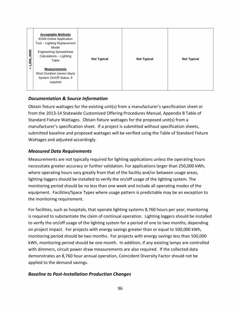
96

> 1,

000,

.000

0




Table










97






Operating Hours


98






All fixtures must comply with Title 10 of the Code of Federal Regulations as well as California’s Title 24 Regulations.








99


8) Area/Category



9) Tailored Method











Where;


FW = fixture kW





100












Where;







101








Where;


FW = fixture kW




Given:

Building Type: Storage, conditioned






102





[ ] [ ]( ) [ ] 8.208/00421.0300,51890,100]_[__ −=−×−= kWhthermkWhkWhkWhSavingsThermAnnual

Note that demand savings should be calculated using the DEER Peak method.Please reference section, Calculating DEER Peak Estimation Methods, for additional details regarding the recommended approaches for determining eligible demand savings.

103

LIGHTING – LED

EEM Description: Replacement of existing lamps and fixtures with LED units of higher efficacy. Work or Product: Lumens Load Influences: None (load influences would only occur in measures involving lighting controls, which is considered a separate EEM) Measures that include de-lamping are addressed in the Production Changes section below. Performance Influences: None

<= Im

pact

kW

h/yr

Constant Load?

Yes No


Yes No Yes No

0 to

250

,000

Acceptable Methods




Measurements

None


250,

000

to 1

,000

,000




Table




104

> 1,

000,

.000

0




Table





Obtain fixture wattages for the existing unit(s) from a manufacturer’s specification sheet or from the 2013-14 Statewide Customized Offering Procedures Manual, Appendix B Table of Standard Fixture Wattages. If a project is submitted without specification sheets, submitted baseline wattages will be verified using the Table of Standard Fixture Wattages and adjusted accordingly. Obtain fixture wattages for the proposed unit from a manufacturer’s specification sheet, LM-79 Testing Report, EnergyStar, or from Design Lights Consortium (DLC).



For facilities, such as hospitals, that operate lighting systems 8,760 hours per year, monitoring is required to substantiate the claim of continual operation. Lighting loggers should be installed to verify the on/off usage of the lighting system for a period of three months and electrical panel metering should be conducted for 75 days. In addition, if any existing lamps are controlled with dimmers, circuit power draw measurements are also required. If the collected data demonstrates an 8,760 hour annual operation, Coincident Diversity Factor should not be applied to the demand savings.


105






Operating Hours

System operating hours should, at minimum be calculated based on the existing lighting schedule and in accordance with the existing operating hours of the facility. When not supportable with available data, DEER values by building type should be used as proxies. When appropriate, it is recommended that system operating hours be calculated based on short term

106

monitoring. Lighting loggers should be installed to determine operating hours where lighting schedules vary greatly on a daily basis or fluctuate between usage areas. Please see the Data Requirements section above for further details.





LED fixtures must be specifically listed in or comply with the testing standard requirements described in the 2013-14 Statewide Customized Offering Procedures Manual for Business, Appendix E, where Table E1 includes approved EnergyStar rated, DLC qualified, and Utility qualified LED fixtures. Integral LED lamps must be specifically listed in or comply with the testing standards and requirements described in Appendix F. Table F1 includes DLC and IOUqualified integral LED lamps.

EnergyStar - http://www.energystar.gov/index.cfm?c=ssl.pr_commercial

DesignLights Consortium - http://www.designlights.org

LED retrofit kits include installing a new ballast, socket, reflector, and LED modular strip. LED retrofit kits MUST follow the identified criteria. In addition to DLC retrofit criteria:

1. All existing interconnects, sockets, and ballasts must be removed from existing fixture, in accordance with T24 2013

2. All LED kits should be hard-wired, in accordance with IOU policy

3. For Linear Fluorescent retrofits, LED retrofit kits need comparable dimming capability – should follow the minimum T24 requirements for its baseline application

http://www.energystar.gov/index.cfm?c=ssl.pr_commercial%20�

http://www.designlights.org/�

107








11) Area/Category



12) Tailored Method










108


Where;


FW = fixture kW
















Where;


109


Calculated projects must use the CFL interactive effects and CDF (in lieu of non-CFL) for the LED screw in lamps. The CFL IEs and CDFs should be applied to all the screw-in, A-base fixtures, both the screw-in lamp baseline and the screw-in LED measure.












Where;


FW = fixture kW


110



Given:

Building Type: Grocery


Baseline Usage (kWh): 5,793.8


Proposed Usage (kWh): 3,928.0




[ ] [ ]( ) [ ] 1.959,1/05.10.928,38.793,5]_[__ =×−= kWhkWhkWhkWhkWhSavingsEnergyAnnual


[ ] [ ]( ) [ ] 4.22/012.00.928,38.793,5]_[__ −=−×−= kWhthermkWhkWhkWhSavingsThermAnnual


111

LIGHTING – COMPACT FLUORESCENT FIXTURES RETROFITS

EEM Description: Replacement of existing lamps and fixtures with CFL units of higher efficacy. Work or Product: Lumens Load Influences: None (load influences would only occur in measures involving lighting controls, which is considered a separate EEM) Measures that include de-lamping are addressed in the Production Changes section below. Performance Influences: None

<= Im

pact

kW

h/yr

Constant Load?

Yes No


Yes No Yes No

0 to

250

,000

Acceptable Methods




Measurements

None


250,

000

to 1

,000

,000




Table




112

> 1,

000,

.000

0




Table








For facilities, such as hospitals, that operate lighting systems 8,760 hours per year, monitoring is required to substantiate the claim of continual operation. Lighting loggers should be installed to verify the on/off usage of the lighting system for a period of three months and electrical panel metering should be conducted for 75 days. In addition, if any existing lamps are controlled with dimmers, circuit power draw measurements are also required. If the collected data demonstrates an 8,760 hour annual operation, Coincident Diversity Factor should not be applied to the demand savings.


113






Operating Hours


114





All fixtures must comply with Title 10 of the Code of Federal Regulations (same as CWT) as well as California’s Title 24 Regulations. Compact fluorescent lamps must be equipped with electronic ballasts. Screw-in lamps CFLs are not eligible for Statewide Customized Offering incentives.









14) Area/Category

115



15) Tailored Method











Where;


FW = fixture kW







116










Where;







117








Where;


FW = fixture kW




Given:

Building Type: Retail, small





DEER Interactive Effects (DIE): 1.14 kWh/kWh, 1.3 kW/kW, -.0.0013 therm/kWh

118





[ ] [ ]( ) [ ] 6.26/0013.0624,9075,30]_[__ −=−×−= kWhthermkWhkWhkWhSavingsThermAnnual


119

LIGHTING CONTROLS – OCCUPANCY SENSORS (LT-43077)

EEM Description: Addition of occupancy sensor(s) to existing lighting fixtures or to proposed lighting fixtures as part of a lighting retrofit. Work or Product: Lumens Load Parameters: Human occupancy Performance Influences: None. It is assumed that the controlled fixtures operate in ON/OFF fashion

<= Im

pact

kW

h/yr

Constant Load?

Yes No


Yes No Yes No

0 to

250

,000

Not Typical

Not Typical

Acceptable Methods

IDSM Online Application Tool – Lighting Controls

Engineering Spreadsheet Calculations – Lighting Table

Measurements

Short Duration (seven days) System On/Off Status

System Power (for kW)

Not Typical

250,

000

to 1

,000

,000

Not Typical Not Typical

Acceptable Methods



Measurements



Not Typical

> 1,

000,

.000

0

Not Typical

Not Typical

Acceptable Methods



Measurements



Not Typical

120


A manufacturer’s specification sheet should be obtained to verify the input wattage of the controlled lighting fixtures (ballast and lamp, if applicable). If a project is submitted without specification sheets, submitted fixture wattages will be verified using the 2013-14 Statewide Customized Offering Procedures Manual, Appendices B – Table of Standard Fixture Wattages, E – Table of Pre-Qualified LED Fixtures, and F – Table of Pre-Qualified Integral Led Lamps and adjusted accordingly. Operating specifications for the proposed occupancy sensors should be obtained from a manufacturer’s specification sheet.


If neither of the methods mentioned in the Reasonable Assumptions section are suitable for estimating savings, an alternate method may be utilized in which reduction in lighting operating time is defined by pre- and post-installation data collection. Reduction in lighting demand is based on the difference in the coincident peak demand between the pre-and post-installation conditions. For applications utilizing M&V, at a minimum, lighting loggers (ON/OFF) should be installed on all or a sample of the fixtures in question to verify actual operation. The monitoring period should be no less than one week and should include all operating modes of the equipment. The analysis should determine the estimated reduction in operating time due to the occupancy sensors for the same schedule. This approach can only be utilized if energy savings are to be claimed. The sampling rate should be no longer than hourly.

For demand reduction, kWh meters shall be installed on all or a sample of the fixtures in question to verify actual demand reduction. Analysis should determine the estimated reduction in coincident peak due to the occupancy sensors for the same schedule. The analysis should also determine the estimated reduction in operating time due to the occupancy sensors for the same schedule. A 15 minute data sampling rate is recommended.

Data sampling can be employed when there are a significant number of different areas to monitor. Sampling should follow the requirements outlined in the Sampling section on page 55 of this document.

If an existing study that contains data similar to the M&V requirements is available for the same building type, occupancy, and usage, it can be submitted and reviewed to address the M&V approach. If this option is selected, the M&V plan will require Energy Division staff review and approval prior to any work commencing.

121


The work product (lumens) of the system is reduced through the implementation of occupancy sensors. The required amount of illumination is still provided in the post-installation condition, but fixtures are de-energized when they are not required.

If the lighting requirements of the facility are changed from the baseline condition, then the most current operating schedule is to be used in the savings calculations. An example of this situation would be the addition of a second shift in a manufacturing facility. This schedule change would by increase the amount of time that lighting fixtures would operate in a theoretical baseline situation.


In order for a project to be eligible for the Statewide Customized Offering, any existing equipment required to establish the project baseline must be operating and available for inspection. If, at the time of pre-installation inspection, less than 10% of the controlled lighting fixtures include burned out lamps, they may be counted and included when calculating the energy associated with the baseline system. However, if more than 10% of the fixtures house burned out lamps, or if the fixtures are found to be non-operational, those fixtures will not be considered eligible when determining the baseline energy usage. The proposed occupancy sensors cannot be installed or on site in the baseline condition.

Lighting fixtures that are controlled with broken or malfunctioning sensors in the baseline condition are not eligible for energy savings incentives.

This measure is typically considered a Retrofit Add-on (REA) and as such a single baseline for the control system should be used. In most cases the simple addition would not trigger code, and thus the baseline is the existing piece of equipment. However, the upcoming 2013 Title 24 will mandate lighting occupancy sensors with most lighting retrofits. As such, effective July 1, 2014, most lighting projects will need to account for occupancy sensors in the code baseline. It should be noted, though, that Title 24 includes some exceptions to this mandatory requirement.

Operating Hours

Baseline system operating hours should, at minimum be estimated based on the existing lighting schedule and in accordance with the existing operating hours of the facility. When not supportable with available data, DEER values by building type should be used as proxies. If the

122

M&V method is chosen to estimate energy savings associated with occupancy sensors, system operating hours (pre and post) may be calculated based on short term monitoring. Lighting loggers (ON/OFF) should be installed to determine operating hours.

Please note that the baseline operating hours must be reasonable. Baseline fixture operating hours should correspond with the occupancy hours of the facility, with the exception of emergency lighting such as exit signs.


As of February 15, 2013, Table 2-1, Section 2 of the 2013 Statewide Customized Offering Procedures Manual for Business reduction rates in operating time for occupancy sensors relating to various space types can no longer be utilized in energy savings calculations for occupancy measures.

Reasonable methods to estimate energy savings associated with occupancy sensors are provided below. These reduction rates can be utilized in calculations in lieu of measurement data or other documentation to verify the reduction in operating hours.

1. The first approach assumes that occupancy sensors deliver (a) 15% reduction or less in lighting operating time (energy savings), and (b) 0% reduction in peak demand. This assumption applies to all building types and may only be used to estimate annual energy saved. For this method, M&V is not required to validate annual energy saved.

2. The second approach utilizes the DEER methodology. DEER methodology includes an

acceptable percent reduction of full load hours and fractions of full load hour reductions for weekday and weekend open and closed periods based on DEER building. DEER assumptions are limited to the building types listed in the DEER spreadsheet. The DEER methodology is acceptable to estimate annual energy saved and peak demand reduction. The appropriate DEER approach should be referenced in the calculations. The DEER methodology only applies to interior applications. For exterior applications, the Applicant may either assume 15% reduction in operating time or perform measurement and verification. However, M&V is not required if DEER methodology is used. Additionally, note that the DEER Demand Direct Impact kW Reduction factor already accounts for Coincident Diversity Factor.


123

For wireless, battery-powered, lighting controls and sensors:

1. The battery-powered wireless devices must be supplied with an active feedback system that provides an alarm/clear notification when the unit's battery is low and requires replacement.

2. The EUL will be the battery life in years divided by two.

3. The minimum battery life must be at least 5 years (or longer) to qualify for an incentive. A third party test is required to verify the battery life.


The energy savings for occupancy sensors stem from a reduction in the existing lighting system operating hours. Therefore, the energy savings are calculated by applying the fixture kW to the reduction in hours. If the project also involves a fixture efficiency improvement, then the replacement kW should be used to estimate the savings.

Given:

Building Type: Assembly, conditioned

Controlled Wattage: 10,000

Annual Hours of Use: 4,380

DEER Interactive Effects (DIE): 1.13 kWh/kWh, 1.22 kW/kW, -0.0041 therm/kwh


DEER Energy Use Direct Impact (EUDI), [kWh]: 0.2

DEER Demand Direct Impact (DDI), [kW]: 0.077

The annual energy savings estimate assuming a 15% reduction in operating time is calculated as follows:

×××=

kWhHoursWatt

DIEUseofHoursAnnualWattageControlledkWhSavingsEnergyAnnual_000,1

15.0____]_[__

[ ] [ ] [ ]kWh

kWhHoursWatt

HoursWattskWhSavingsEnergyAnnual 1.424,7_000,1

15.013.1380,4000,10]_[__ =

×××=

Note that if this approach is used, no reduction in peak demand may be claimed.

124

The annual energy and demand savings estimates assuming DEER Methodology is calculated as follows:

×××=

kWhHoursWatt

EUDIDIEUseofHoursAnnualWattageControlledkWhSavingsEnergyAnnual_000,1

____]_[__

[ ] [ ] [ ]kWh

kWhHoursWatt

HoursWattskWhSavingsEnergyAnnual 8.898,9_000,1

2.013.1380,4000,10]_[__ =

×××=

××=

kWWatts

DDIDIEWattageControlledkWSavingsDemand000,1

_]_[_

[ ] [ ]kW

kWWatts

WattskWSavingsDemand 94.0000,1

077.022.1000,10]_[_ =

××=

Since the Demand Direct Impact already includes Coincident Diversity Factor, the Coincident Diversity Factor is not applied again to the Total Peak Reduction calculation.

×××=

kWhHoursWatt

EUDIDIEUseofHoursAnnualWattageControlledthermsSavingsThermAnnual_000,1

____]_[__

[ ] [ ] [ ] [ ]therms

kWhHoursWatt

kWhthermHoursWattsthermsSavingsThermAnnual 92.35_000,1

2.0/0038.0380,4000,10]_[__ −=

×−××=

Annual therm savings should only be calculated for sites that have a natural gas heater.

125

LIGHTING CONTROLS – DAY LIGHTING (LT-90853& LT-74751)

EEM Description: The installation of photocells to existing lighting fixtures or to proposed lighting fixtures as part of a lighting retrofit. The fixtures may or may not contain dimmable ballasts. Work or Product: Lumens Load Parameters: Ambient daylight conditions Performance Influences: The input power of dimmable ballasts fixtures varies with efficacy.

<= Im

pact

kW

h/yr

Constant Load?

Yes No


Yes No Yes No (Dimmable Ballasts)

0 to

250

,000

Not Typical

Not Typical

Acceptable Methods eQUEST – Lighting Controls

EEM Engage 2008 – Daylighting

Controls Superlite 2.0 Skycalc v3.0

Measurements

None




Measurements

None

250,

000

to 1

,000

,000





Measurements


System Amperage

Acceptable Methods

eQUEST – Lighting Controls EEM

Engage 2008 – Daylighting Controls

Superlite 2.0 Skycalc v3.0

Measurements


System Amperage

> 1,

000,

.000

0

Not Typical

Not Typical





System Power

Acceptable Methods

eQUEST – Lighting Controls EEM

Engage 2008 – Daylighting Controls

Superlite 2.0 Skycalc v3.0


System Power

126


A manufacturer’s specification sheet should be obtained to verify the input wattage of the controlled lighting fixtures. If a project is submitted without specification sheets, submitted fixture wattages will be verified using the 2013-14 Statewide Customized Offering Procedures Manual, Appendix B Table of Standard Fixture Wattages and adjusted accordingly. Operating specifications for the proposed photo cells and lighting control system should be obtained from manufacturer’s specifications. The documentation should include the type of control strategy to be utilized in the proposed system (ON/OFF, Continuous, Stepped, etc).

If the system will utilize dimmable ballasts, then the appropriate specification sheets should be provided to substantiate the power demand of the lighting fixtures at part loads.


Measurements are not typically required for day lighting control applications unless the suggested baseline operating hours necessitate greater accuracy or further validation. For applications larger than 250,000 kWh, where operating hours vary greatly from that of the facility and/or between usage areas, or where the lighting controls operation is questionable or complicated, lighting loggers (ON/OFF) should be installed on the fixtures in question to verify actual operation. The monitoring period should be no less than one week and include all operating modes of the equipment. Amperage data should be recorded if lighting loggers (ON/OFF) are deemed insufficient in verifying the lighting system operation. True RMS power measurements should be taken for projects over 1,000,000 kWh.

Measurements may also be required to verify the power draw of lighting fixtures with dimmable ballasts. Spot measurements in amperage or kW may be appropriate or short term monitoring may be required that includes all operating modes of the equipment.

Lighting set points may be verified with spot measurements of light levels (lumens/foot candles).


The work product (lumens) of the system is reduced through the implementation of a daylighting control system. The required amount of illumination is still provided in the post-installation condition, however some (or all) of this load may be supplied by natural light. The input power to lighting fixtures may be reduced or eliminated in these conditions.

If the lighting requirements of the facility are changed from the baseline condition, then the latest operating schedule is to be used in the savings calculations. An example of this situation would be the addition of a second shift in a manufacturing facility. This schedule change would

127

increase the amount of time that lighting fixtures would operate in a theoretical baseline situation.

The customer is responsible to ensure that adequate lighting levels are maintained. Generally the lumen output of the installed lighting system is not measured except in extreme cases where the lighting level is not reasonable for the intended purpose of the area.


In order for a project to be eligible for the Statewide Customized Offering, any existing equipment required to establish the project baseline must be operating and available for inspection. If, at the time of pre-installation inspection, less than 10% of the controlled lighting fixtures include burned out lamps, they may be counted and included when calculating the energy associated with the baseline system. However, if more than 10% of the fixtures house burned out lamps, or if the fixtures are found to be non-operational, those fixtures will not be considered eligible when determining the baseline energy usage. The proposed occupancy sensors cannot be installed or on site in the baseline condition.

Lighting fixtures that are controlled with broken or malfunctioning photo sensor controls in the baseline condition are not eligible for energy savings incentives.

This measure is typically considered a Retrofit Add-on (REA) and as such a single baseline for the control system should be used. In most cases the simple addition would not trigger code, and thus the baseline is the existing piece of equipment. However, the upcoming 2013 Title 24 will mandate lighting occupancy sensors with most lighting retrofits. As such, effective July 1, 2014, most lighting projects will need to account for occupancy sensors in the code baseline. It should be noted, though, that Title 24 includes some exceptions to this mandatory requirement.

Operating Hours

Baseline system operating hours should, at minimum be estimated based on the existing lighting schedule and in accordance with the existing operating hours of the facility. When not supportable with available data, DEER values by building type should be used as proxies. When appropriate, it is recommended that baseline system operating hours be calculated based on short term monitoring. Lighting loggers (ON/OFF) should be installed to determine operating hours where lighting schedules vary greatly on a daily basis or fluctuate between usage areas. (For applications greater than 250,000 kWh, where operating hours vary greatly from that of the facility and/or between usage areas.)

The proposed operating hours should be determined an accepted modeling program.

128


Assumptions regarding facility space type can be made to match that of DEER Model building. Skylight specifications (Ufactor, SHGC, and Transmittance) may be assumed in lieu of available specification sheets.

If the proposed day lighting project consists of photo sensors for fully exposed outdoor fixtures (sensors), it is reasonable to assume an operation of 12 hours per day in the post-installation case.


There is no minimum lumen requirement or lighting standard set by the Customized Offering Program. The lighting set points on most daylighting control systems are programmed manually based on a lighting level deemed appropriate by site personnel.

For wireless, battery-powered, lighting controls and sensors:

1. The battery-powered wireless devices must be supplied with an active feedback system that provides an alarm/clear notification when the unit's battery is low and requires replacement.

2. The EUL will be the battery life in years divided by two.

3. The minimum battery life must be at least 5 years (or longer) to qualify for an incentive. A third party test is required to verify the battery life.


In most cases, the energy savings for daylighting projects should be calculated using an energy modeling tool that accounts for annual climate zone specific weather data. This data is used to determine the amount of natural light available to be captured based on the attributes of the facility. The lighting levels are then incorporated into the proposed daylighting control strategy to determine the amount of energy savings. The following tools are eligible to be used on day lighting control projects:

• eQUEST 3.63– Lighting Controls EEM

• Engage 2008 – Daylighting Controls

• Superlite 2.0

129

• Skycalc v3.0

DEER Peak Demand savings can also calculated by these tools.

Please note that spreadsheet or lighting table calculations may be appropriate for daylighting control projects involving lighting fixtures on a building exterior or fully exposed outdoor parking lot.

130

REFRIGERATION – STRIP CURTAINS

EEM Description: Installation of Strip Curtains in order to decrease infiltration. Work or Product: Tons of Cooling. Load Influences: Insulation efficiency of Strip Curtains, operating schedule, and the number, temperature & humidity of infiltrating air and duration of door openings/closings. Performance Influences: Cooling load level and ambient conditions.

<= Im

pact

kW

h/yr

Constant Load?

Yes No


Yes No Yes No

0 to

250

,000

Not Typical


Acceptable Methods IDSM Online Application Tool

– Rapid Close Doors (Strip Curtain Measure)

Engineering Spreadsheet Calculations

Measurements None

250,

000

to 1

,000

,000



– Rapid Close Doors (Strip Curtain Measure)Engineering

Spreadsheet Calculations Measurements

Refrigeration system power draw and cooling load. Short Term Monitoring (one week).

> 1,

000,

.000

0



– Rapid Close Doors (Strip Curtain Measure)Engineering

Spreadsheet Calculations Measurements

Refrigeration system power draw and cooling load. Short

Term Monitoring (2 – 4 weeks)


Obtain specification sheets for both the existing and proposed Strip Curtains in order to verify insulation properties, U-Factor for example. If baseline equipment exists, but specification sheets cannot be provided, insulation efficiency should be compared to engineering resources or industry standards to determine reasonableness and accuracy. Determine the operating

131

schedule of the facility in order to verify the hours of operation and number of door openings. Gather the refrigeration equipment nameplate power ratings and system cooling capacity in order to determine the interior and exterior refrigeration system efficiencies. If the doorway opens to the outside, only the interior refrigeration system efficiency will be analyzed.


Measurements are not typically required for Strip Curtain applications. For applications larger than 250,000 kWh, the power draw (kW) and cooling load (ton hours) of the refrigeration system should be monitored prior to installation for a minimum of one week in order to determine the system efficiency. The power draw of the system is easily monitored, while the cooling load is not. For larger applications, the facility will generally have a central monitoring system, and trend data for the cooling load should accessible. At a minimum, the cooling capacity and nameplate power ratings for the refrigeration system equipment should be gathered in order to estimate the system efficiency.


Changes to the refrigeration system operating conditions during the installation of the equipment should be reflected in a revised baseline. For example, if a facility decides to stop operation on weekends, the baseline will be revised to reflect these new operating hours.



Operating Hours

Depending on the application, Operating Schedules could vary throughout the year. These schedules should be submitted by the customer and should be supportable.


All doors operating under the same doorway characteristics (similar operating schedules, doorway specifications, traffic flow, etc.) can be grouped into doorway types. Multiple

132

doorway types can be identified and modeled simultaneously using the IDSM Online Application Tool – Rapid Close Door Tool.


None


Strip Curtain retrofits typically save energy by reducing the refrigeration system load due to infiltration. This can be achieved by improving the seal/insulation of the doorway, increasing the door speed and/or reducing the amount of time a door simply stands open.

Detailed energy savings calculations for rapid close doors in Appendix A can be modified for use with strip curtains.

133

REFRIGERATION – DOORS

EEM Description: Installation of increased efficiency Refrigeration Doors in order to decrease infiltration. Work or Product: Tons of Cooling Load Influences: Insulation efficiency of Refrigeration Door, operating schedule, and the number and duration of door openings/closings. Performance Influences: Temperature of infiltrating air, cooling load level and ambient conditions.

<= Im

pact

kW

h/yr

Constant Load?

Yes No


Yes No Yes No

0 to

250

,000

Not Typical



– Rapid Close Doors Engineering Spreadsheet

Calculations Measurements

None

250,

000

to 1

,000

,000





Refrigeration system power draw and cooling load. Short Term Monitoring (one week).

> 1,

000,

.000

0





Refrigeration system power draw and cooling load. Short

Term Monitoring (2 – 4 weeks)

134


Obtain specification sheets for both the existing and proposed refrigeration doors in order to verify insulation properties, U-Factor for example. If specification sheets cannot be provided for the baseline equipment, insulation efficiency should be compared to engineering resources or industry standards to determine reasonableness and accuracy. Determine the operating schedule of the facility in order to verify the hours of operation and number of door openings. Gather the refrigeration equipment nameplate power ratings and system cooling capacity in order to determine the interior and exterior refrigeration system efficiencies. If the doorway opens to the outside, only the interior refrigeration system efficiency will be analyzed.


Measurements are not typically required for Refrigeration Door applications. For applications larger than 250,000 kWh, the power draw (kW) and cooling load (ton hours) of the refrigeration system should be monitored prior to installation for a minimum of one week in order to determine the system efficiency. The power draw of the system is easily monitored, while the cooling load is not. For larger applications, the facility will generally have a central monitoring system, and trend data for the cooling load should accessible. At a minimum, the cooling capacity and nameplate power ratings for the refrigeration system equipment should be gathered in order to estimate the system efficiency.


Changes to the refrigeration system operating conditions during the installation of the equipment should be reflected in a revised baseline. For example, if a facility decides to stop operation on weekends, the baseline will be revised to reflect these new operating hours.


One must first determine if the measure is eligible for early retirement (RET). If the measure does not qualify for early retirement (RET), then a single baseline is determined and must use the forecasted equipment load and an appropriate minimum efficiency standard to establish baseline performance. An acceptable minimum efficiency standard must be a government minimum efficiency standard or, if a minimum standard efficiency is not available, the current industry practice. If early retirement does apply, then two separate baselines must be determined. The first baseline shall be determined using the pre-existing equipment efficiencies. The second baseline shall be determined using forecasted equipment load and an appropriate minimum efficiency. For non-RET, the industry standard is strip curtains.

135

Operating Hours

Depending on the application, Operating Schedules could vary throughout the year. These schedules should be submitted by the customer and should be supportable.


All doors operating under the same doorway characteristics (similar operating schedules, doorway specifications, traffic flow, etc.) can be grouped into doorway types. Multiple doorway types can be identified and modeled simultaneously using the IDSM Online Application Tool – Rapid Close Door Tool.


None


Refrigeration Door retrofits typically save energy by reducing the refrigeration system load due to infiltration of outside air. This can be achieved by improving the seal/insulation of the doorway, increasing the door speed and/or reducing the amount of time a door simply stands open.

Energy savings calculation details may be found in the rapid close door portion of Appendix A

136

REFRIGERATION – MOTORS

EEM Description: Replacement of inefficient fractional horsepower shaded pole or permanent split capacitor (PSC) evaporator fan motors with more efficient electronically commutated motors (ECM) for evaporator fans in refrigerated display cases or walk-in coolers. Work or Product: Tons of cooling Load Influences: Evaporator fan motors for refrigerated display cases and walk-in coolers typically run at full air-flow and constant load. However, there are applications where evaporator fan controllers actuate the motor to operate at reduced speeds (power draw) when the system detects no mass flow (refrigeration compressors cycle off). These systems allow the fans to operate at a high and low speed (2 speeds). Performance Influences: In applications where evaporator fan controllers are implemented, the cycling of the compressors allows the speed of the fan motors to be reduced. This cycling of compressors can be influenced by things such as weather, restocking of items, lighting, and opened refrigerated doors.

<= Im

pact

kW

h/yr

Constant Load?

Yes No


Yes No Yes No

0 to

250

,000

Acceptable Methods


Measurements None

Not Typical

Not Typical

Acceptable Methods


Measurements None

250,

000

to 1

,000

,000

Not Typical Not Typical Not Typical Not Typical

> 1,

000,

.000

0

Not Typical


137


For refrigerated display cases, the number of doors should be counted and the manufacturer/model number should be recorded. Obtaining the specifications for display cases should provide you with the watts/door consumption. The nameplate should also reveal the amperage and voltage of the evaporator fans.

Refrigeration schedules would also provide quantity, voltage and amperage draw of the evaporator fans in addition to the make, model and quantity of doors.

If the system applies evaporator fan controllers, it should be determined which fans are controlled. Evaporator fan controllers allow the speed of a fan motor to be reduced when the load is satisfied and compressors are not activated. Refrigeration system specification and capacity should be obtained and assessed against the load since compressors that are undersized will operate continuously and the controllers will not drop the voltage to the motor. If the system is oversized, the compressors will cycle off more and evaporator fan motors will operate at reduced speeds for longer periods of time. The motor rpm reduction set-point should also be obtained from the customer.


Measurements are not required for this measure


Changes from baseline to post-installation production would occur if the facility has more or less refrigerated display cases or walk-in coolers. The inventory of motors should be carefully counted in the post installation inspections as the production loads will be based on the post-installed number of cases or coolers.



138

Operating Hours

Evaporator fan motors for refrigerated display cases and walk in coolers operate continuously and typically have a duty cycle of 100%. Low-temperature display cases may have a slightly lower duty cycle (96%) due to defrost cycles.


The following assumptions are based on reports that were provided to the Department of Energy. It would be reasonable to assume that evaporator fans operate continuously for refrigerated display cases and walk in coolers. In establishing baseline consumption for systems that implement evaporator controls, it would be reasonable to assume that the compressors operate between 60-70% if they are not undersized.

*Energy Savings Potential and R&D Opportunities for Commercial Refrigeration Final Report, Submitted to: U.S. DOE Energy Efficiency and Renewable Energy Building Technologies Program; Navigant Consulting, Inc. September 23, 2009.

*Energy Savings Potential for Commercial Refrigeration Equipment Final Report; Submitted to: U.S. DOE Building Equipment Division Office of Building Technologies; Arthur D. Little, Inc. June 1996.


If the facility plans to add new load, it may be eligible for incentives if it meets the Statewide Customized Offering Guidelines or is deemed reasonable by the Utility Administrator. Section 1.4.4 New Load Project Eligibility should be reviewed in the 2013-14 Statewide Customized Offering Procedures Manual for Business to determine eligibility.


The following calculation should be used to determine the energy savings for a refrigeration motor project:


QTY x MCFL x OPHR = annual kWh

Medium Temperature Duty Cycle Assumptions DOE A.D. LittleRefrigerated Display Case Evaporators: 100% 100%

Walk in Coolers Evaporators: 100% 100%Walk in Cooler Compressors: 66% 66%

Low Temperature Duty Cycle Assumptions DOE A.D. LittleRefrigerated Display Case Evaporators: 96% 96%

Walk in Freezer Evaporators: 100% 100%Walk in Freezer Compressors: 70% 63%

139

QTY x MCFL = kW

Baseline/Proposed Calculation with Evaporator Fan Controllers

QTY x OPHR X (MCFL X Duty Cycle FL + MCRL X Duty Cycle RL) = annual kWh

QTY x MCFL = kW

Where;

QTY = number of motors

MCFL = Motor consumption at Full Load (kW)

MCRL = Motor consumption at Reduced Load (kW)

OPHR = annual hours of operation (hrs)

Duty Cycle FL = Duty Cycle at Full Load (%)

Duty Cycle RL = Duty Cycle at Reduced Load (%)

The motor consumption at reduced load (sites that apply evaporator controls in the baseline scenario) should be calculated by obtaining the pre-set RPM for low load conditions and applying the affinity laws.


140

REFRIGERATION – CONDENSER (RF-90876)

EEM Description: Air Cooled Condenser measures include replacement of existing air cooled condensers for high efficiency air cooled condensers containing bigger surface area, high efficiency fan motors / inverter duty motors, and controls, which are optimized to yield the best energy operating efficiency. Energy savings are realized due to the fact a bigger size air cooled condenser could operate at a lower saturated condensing temperature or pressure; therefore lowering the system compression ratio or reduced fan energy consumption. Work or Product: Tons of refrigeration Load Influences: Weather (EDBT°F), Saturated condenser temperature, CFM, and Design TD, Evaporator Load, and Heat of Compression. Performance Influences: Weather (EDBT°F), Location (altitude and air flow restriction), and condenser design.

<= Im

pact

kW

h/yr

Constant Load?

Yes No


Yes No Yes No

0 to

250

,000


Acceptable Methods Engineering spreadsheets bin analysis & regression

analysis calculations eQuest Refrigeration

Measurements

Short Duration Fan Motor(s) Power Consumption, Cooling

Load & Outside Air Temperature

(Duration will depend on variability in performance &

load – 1 week)

250,

000

to 1

,000

,000



calculations eQuest Refrigeration

Measurements Extended Duration Fan

Motor(s) Power Consumption, Cooling Load & Outside Air Temperature (Duration will depend on

variability in performance & load – 2-4 weeks)

141

> 1,

000,

.000

0



calculations eQuest Refrigeration

Measurements

Extended Duration Fan Motor(s) Power

Consumption, Cooling Load & Outside Air Temperature (Duration will depend on

variability in performance & load – 4 weeks)


Obtain air cooled condenser product data specifications from customer/project sponsor. If product data is not available from either one of them, then please contact the original equipment manufacturer (OEM). When applicable, attain process flow diagrams of the affected system.

Air cooled condenser product data specifications should contain the following information:

• THR Capacity: (MBH, Tons, BTUH)

• Design Air flow: CFM

• Design TD

• Fan configuration

• Number of fans

• Fan motor specifications

• Control mechanism types : o Variable Condenser Fan Speed Control o Condenser Fan Cycling o Split or Multi Circuit Condenser System o “Flooded” Head Pressure Control


If baseline could not be established with exactness due to the lack of product data specifications and unknown operating number of hours, the following should be done:

Voltage, current, and power factor measurements on energy consuming components are required to calculate energy consumption (kWh) and energy demand (kW). The monitoring period would depend on the magnitude of customer’s energy impact (kWh/yr). This goes generally from one week to four weeks.

142

The above is also mandatory and applicable to larger applications (>250,000 kWh) where the load and/or performance would vary based on weather conditions; therefore the trend monitored data should display power consumed by the pertinent equipment and outdoor air temperatures.


In cases where there is an increase/decrease in load due to production, or contraction /expansion on a facility, the reviewer will have to use the following approach to calculate the energy savings:

The baseline energy use is based on the current production or thermal load and equipment current power consumption.

The proposed load is assumed to be based on the current production or thermal load and current power consumption versus the forecasted production and/or increase/ decrease in building load.

The production (+/-) or load (+/-) could be verified through production logs and equipment run time monitoring during the installation review phase.


In order for a project to be eligible for the Statewide Customized Offering, any existing equipment required to establish the project baseline must be operating and available for inspection. Moreover, the equipment must be running and in good conditions at the time of inspection. The nameplate rate performance of the existing equipment is used to define baseline heat rejection equipment performance, where applicable.


143

Operating Hours

System operating hours should be determined based on equipment operation schedule or existing operating hours of the facility. This critical information could also be verified with the use of data loggers.


Air cooled condenser operate at different design TD’s based on their application. For example:

Air Conditioning = 25°F to 30°F TD

Refrigeration:

• Medium Temperature = 15°F TD

• Low Temperature = 10°F TD

TD = Temperature Difference = Saturated Condensing Temperature (SCT°F) – Ambient Temperature (DBT°F)


Noise reduction, reduced fan motor watts, and fin spacing are considered special requirements. There are applications of air cooled condensers in high dust or dirt areas in which wider fin spacing is required to prevent the coils from being blocked.

If an air cooled condenser is retrofitted to a water cooled condenser, the following design parameters need to be taken into consideration:

• Inlet fluid temperature – °F

• Condensing Refrigerant Temperature - °F

• Fouling factor (0.00025 ARI Standard)

• Total Heat of Rejection (THR) - BTUH Refrigerant

• Fluid Side Pressure Drop (PSI)

• Pump selection


144

Develop a regression analysis based on logged and collected data in conjunction with weather bin temperature data (DBT°F for air cooled condensers, and WBT°F for evaporative condensers).

145


EEM Description: Replacement of existing evaporative condensers with oversized and high efficiency evaporative condensers containing high efficiency inverter duty fan motors for capacity control, and high efficiency basin water pump. Energy Savings: are realized due to the fact that evaporative condensers provide a lower condensing temperature than a dry-air cooled condenser because of the evaporative effect of the sprays. Work or Product: Tons of refrigeration Load Influences: Weather (reduced WBT°F), lightened loads and capacity control Performance Influences: Weather (EWBT°F), location (altitude and air flow restriction), and scaling.

<= Im

pact

kW

h/yr

Constant Load?

Yes No


Yes No Yes No

0 to

250

,000


Acceptable Methods

Engineering spreadsheets bin analysis & regression


Measurements

Short Duration Fan Motor(s) Power Consumption, Water Pump Consumption & OAT’s


load – 1 week)

250,

000

to 1

,000

,000




Measurements

Extended Duration Fan Motor(s) and Water Pump

Power Consumption Monitoring & OAT’s


load – 2 - 4 weeks)

146

> 1,

000,

.000

0




Measurements Extended Duration Fan

Motor(s) and Water Pump Power Consumption Monitoring & OAT’s


load – 4 weeks)


Obtain evaporative condenser product data specifications from customer/project sponsor. If product data is not available from either one of them, then please contact the original equipment manufacturer (OEM). When applicable, attain process flow diagrams of the affected system.

Evaporative condenser product data specifications should contain the following information:

• Capacity: THR (MBH, Tons, BTUH)

• Design WBT°F

• Fan type (centrifugal or propeller)

• Number of fans

• Fan motor specifications

• Sump pump motor specifications

• Control mechanism types: o Variable Condenser Fan Speed Control o Condenser Fan Cycling o Two speed fan motors o Modulating fan discharge dampers




147



In cases where there is an increase/decrease in load due to production or contraction/expansion of a facility, the reviewer will have to use the described below approach to calculate the energy savings.

For retrofit of existing/systems with different capacity equipment than the baseline or post-installation production levels are different (i.e. the equipment load is higher or lower), the annual energy savings will be calculated assuming the post-installation production or load. The general equation for calculating savings with changes in production is:

Eligible Energy Savings (kWh/year) = (Baseline Efficiency – Proposed Efficiency) x Proposed Production rate or Load x Proposed Operating Hours.


In order for a project to be eligible for the Statewide Customized Offering, any existing equipment required to establish the project baseline must be operating and available for inspection. Moreover, the equipment must be running and in good condition at the time of the inspection. The nameplate rate performance of the existing equipment is used to define baseline heat rejection equipment performance, where applicable.


Operating Hours


148


None


None


Estimations can be performed using bin methods with historical ambient temperature (WBT or DBT depending on type of condenser). More detailed analysis can be performed using one of the preferred building energy modeling tools such as eQuest. M&V can be performed by developing a regression analysis based on logged data in conjunction with corresponding climate zone weather bin temperature data (WBT°F for evaporative condensers).

149


EEM Description: Replacement of existing shell and tube water cooled condensers with oversized and optimized water cooled condenser, or with brazed plate heat exchangers or semi-welded plate heat exchangers if application permits it. Energy Savings: are realized due to the fact that water cooled condensers provide a lower condensing temperature than dry air-cooled condensers. Work or Product: Tons of refrigeration Load Influences: Entering condenser water temperature (ECWT°F), saturated condensing temperature (SCT°F) Performance Influences: Entering condenser water temperature, fluid volumetric flow rate (gpm), fluid side pressure drop, # of passes, and fouling factor.

<= Im

pact

kW

h/yr

Constant Load?

Yes No


Yes No Yes No

0 to

250

,000




Measurements Short Duration

Compressor(s) Power Consumption, Evaporator Fan Motor(s) and Pump

Power Consumption (Duration will depend on

variability in performance & load – 1 week)

250,

000

to 1

,000

,000




Measurements Extended duration

compressor(s) power consumption, evaporator fan

motor(s) and pump power Consumption


load – 2 - 4 weeks)

150

> 1,

000,

.000

0




Measurements

Extended duration compressor(s) power

consumption, evaporator fan motor(s) and pump power

consumption (Duration will depend on

variability in performance & load - 4 weeks)


Obtain water cooled condenser product data specifications from customer/project sponsor. If product data is not available from either one of them, then, please contact the original equipment manufacturer (OEM). When applicable, attain process flow diagrams of the affected system.

Water cooled condenser product data specifications should contain the following information:

• Inlet fluid temperature – °F

• Condensing Refrigerant Temperature - °F

• Fouling factor (0.00025 ARI Standard)

• Total Heat of Rejection (THR) – BTUH

• Refrigerant Type

• Fluid Side Pressure Drop (PSI)




The above is also mandatory and applicable to larger applications (>250,000 kWh) where the load and/or performance would vary based on weather conditions; therefore the trend

151

monitored data should display power consumed by the pertinent equipment and outdoor air temperatures.



For retrofit of existing/systems with different capacity equipment than the baseline or post-installation production levels are different (i.e. the equipment load is higher or lower), the annual energy savings will be calculated assuming the post-installation production load or load system. The general equation for calculating savings with changes in production is:

Eligible Energy Savings (kWh/yr) = (Baseline Efficiency – Proposed Efficiency) x Proposed Production rate or Load x Proposed Operating Hours.


In order for a project to be eligible for the Statewide Customized Offering, any existing equipment required to establish the project baseline must be operating and available for inspection. Moreover, the equipment must be running and in good condition at the time of the inspection. The nameplate rate performance of the existing equipment is used to define baseline heat rejection equipment performance, where applicable.


Operating Hours


152


If maintained properly, it can be assumed that it is operating efficiently. On the contrary, poor maintenance implies increase power consumption on compressor(s).


Some of the special requirements for water cooled condensers are as follows:

• Fluid type to be used for condensation

• Number of passes

• Fluid side pressure drop

• Marine application (construction material) – most common in refrigeration application than air conditioning application.

• Single circuit or dual circuit


Develop a regression analysis based on logged data in conjunction with corresponding climate zone weather bin temperature data.

eQuest can be used to calculate energy savings in a chilled water plant system where water cooled condensers are used.

eQuest (kW/TR)_Centralized water system = ∑Compressor(s) (kW/TR)+ Chilled water pump(s) (kW/TR)+ Condenser water pump(s) (kW/TR) + Cooling tower fan(s) (kW/TR)

153

REFRIGERATION – COMPRESSOR

EEM Description: Replacement of existing refrigeration compressor with a new higher efficiency compressor, addition of sequencing controls for optimal loading of multiple compressor refrigeration systems and/or installing VFD. Work or Product: Tons of cooling Load Influences: Outdoor ambient conditions, characteristics and mass of material being refrigerated, product entering and set point temperatures of refrigerated space or the coil discharge air, occupancy, internal heat sources, building envelope insulation and infiltration. Performance Influences: Ambient temperature, control strategy, refrigerant type, compressor staging (for multiple units), TXV operation, condenser temp reset and proper commissioning of equipment

<= Im

pact

kW

h/yr

Constant Load?

Yes No


Yes No Yes No

0 to

250

,000

Not Typical

Acceptable Methods Engineering Spreadsheet

Calculations Emerson Product Selection & Energy Analysis Software

Measurements

Spot Measurement Production rate (mass of

product) Electric demand (kW)

Not Typical


Calculations Emerson Product Selection &

Energy Analysis Software

Measurements Spot Measurement

Production rate (mass of product)

Electric demand (kW)

250,

000

to 1

,000

,000

Not Typical


Calculations

Measurements Short term (seven days minimum, sufficient to capture any production

cycle) Production rate (mass of


Not Typical


Calculations

Measurements Short term (seven days minimum, sufficient to

capture any production cycle) Production rate (mass of


154

> 1,

000,

.000

0

Not Typical


Calculations

Measurements Medium term (one month

minimum, sufficient to capture any production



Not Typical


Calculations


minimum, sufficient to capture any production cycle)




Obtain manufacturer’s specifications, if available, for both existing and retrofit equipment. These specifications should include:

• Manufacturer

• Compressor type

• Control type (load/unload, inlet modulation, VFD, etc.)

• Drive motor nameplate rating

• Compressor performance curves

• Total refrigeration system power at rated capacity and full load operating pressure

If the equipment is purchased as a standard package this information will probably be available. For built up systems, try to obtain the design specifications for the system. Also, customer needs to provide the invoices including a detailed breakdown of project costs (i.e. installation, equipment removal, worker and engineering labor costs) at Installation Review (IR) stage of project. When applicable, attain process flow diagrams of the affected system.


Measurements will be required to establish the post-installation operation and to verify savings after the measure is completed. The minimum monitoring period should be no less than two weeks and will increase for larger applications as defined in the above measure table. This data monitoring (cooling load of the system, compressor and condenser fan power, dry bulb and wet bulb temperatures) should be measured to verify system performance and to determine load profile. This measurement needs to be conducted in both the pre and post installation cases to verify the energy model.

155


If the production rate and/or product characteristics are not constant, then the baseline monitoring period must be of sufficient length to capture all potential variations. Baseline energy intensity should then be correlated to both production rate and type of product, and the baseline adjusted to correspond to the measured post-installation production.



Operating Hours

System operating hours for the pre-installation estimate may be based on operation observed during the baseline period. For final savings estimates, operating hours should be based on the operating hours observed during the post-installation monitoring period, and should also take into account any expected variations in schedule or production over the first year of post-installation operation.


None


None


The following calculation should be used to determine energy savings:

Energy Savings = Baseline Energy – Reporting Period Energy ± Adjustments

Where;

156

Baseline Energy = Baseline Intensity (kWh/kg product) * Baseline Production Rate (kg/hr) * Annual Operating Hours

Reporting Period Energy = Reporting Period Intensity (kWh/kg product) * Reporting Period Production Rate (kg/hr) * Annual Operating Hours

Adjustments = Any adjustments required to make the baseline period conditions and production equal to the reporting period conditions and production.

Since 12 months of data collection in either the baseline or post-installation (reporting) period is unlikely, a binned approach, using ambient temperature bins, should be employed in both the pre-installation estimate and the final verified energy savings calculation.

Equipment performance may depend on the characteristics of the product being stored or chilled and the ambient temperature under which the compressor(s) will operate. Energy intensity (kWh/kg of product) must be evaluated for both the “pre” and “post” systems and correlated to ambient temperature using a “binned” approach. Appropriate length of the verification period and required data rate will depend on the process in question. If the system is serving a batch chilling process, energy intensity will need to be analyzed on the basis of the mass of product, dwell time and kWh used for each batch.

Please refer to Appendix A for guidelines in preparing the savings estimate using engineering calculations.

157

REFRIGERATION – SYSTEMS (RF-16859)

EEM Description: Reduced Load on Refrigeration System- Increased Condenser Capacity Work or Product: Tons of refrigeration Load Influences: Load has a significant influence on refrigeration systems. Load can vary because of climate conditions (a warehouse has more heat gain in the summer than in the winter) and/or because of the production type (a warehouse that processes produce will have spikes of load in the late summer and early fall). The load influences the efficiency of the refrigeration system including the compressor(s) and mostly all other auxiliary components. The efficiency of the compressor(s) is based on its differential pressure. Performance Influences: The performance of a refrigeration system can vary significantly based on load (as already described) and on climate conditions. The climate conditions affect the compressor performance by requiring a higher discharge during hotter ambient temperatures. The condenser(s)’ ability to reject heat depends on the ambient conditions too. By oversizing the condenser it is able to reject more heat allowing the compressor to discharge at low pressures however the system will consume more fan energy.

<= Im

pact

kW

h/yr

Constant Load?

Yes No


Yes No Yes No

0 to

250

,000

Not Typical


Bin Analysis Calculations or eQUEST refrigeration

Measurements

Spot measurement of compressor, condenser, and

evaporator

Not Typical

Acceptable Methods Engineering Spreadsheet Bin

Analysis Calculations or eQUEST refrigeration

Measurements


evaporator

250,

000

to 1

,000

,000

Not Typical



Measurements

Compressor, condenser, and evaporator power: short term monitoring for one or

two weeks

Not Typical



Measurements

Compressor, condenser, and evaporator power: short term

monitoring for one or two weeks

158

> 1,

000,

.000

0

Not Typical



Measurements

Compressor, condenser, and evaporator power :

short term monitoring for two to four weeks

Not Typical



Measurements

Compressor, condenser, and evaporator power : short term monitoring for two to

four weeks

Documentation & Source Information Obtain manufacturer specs sheets of the baseline and proposed component involved, at least compressor(s) and condenser(s). In the specs the reviewer needs to find capacity in ton or BTU/hr, power requirement, suction and discharge temperatures/pressures and any other information that can lead to determine the capacity and efficiency of the system and its components. If the specs sheet of the baseline equipment has been lost, which often happens for the 15 year or older equipment, the nameplates of the equipment can be used. In particular HP, kW, suction and discharge pressures or temperatures read from the gauges. Facility production logs, or operations information should also be collected to confirm the yearly operation of the facility and to establish a load profile. When applicable, attain process flow diagrams of the affected system.

Measured Data Requirements Measurements are required to understand load and operation of the systems always in the pre installation inspection and preferably in the post installation as well, unless the control panel clearly shows the important parameters: load and power. For small applications (<250,000 kWh savings) a spot measurement of true power can be sufficient to confirm the power assumptions based on the nameplate information. For larger application (>250,000 kWh savings) where usually the performance of the systems vary depending on the climate conditions trend data are needed. Trend data should show power absorbed by compressors, power absorbed by the condenser, refrigeration delivered, suction and discharge temperature/pressures, outside air temperature and relative humidity. The trend duration should reflect the accuracy required: generally trends go from one week to four weeks (a.k.a. short term monitoring).

Baseline to Post-Installation Production Changes Often such system retrofits happen when the customer is planning to expand the operations. In such case, the reviewer has to apply the current performance to the proposed load which will mean a greater compressor(s) load than during the pre-installation observation. The proposed load is assumed based on the current production and current consumption versus the

159

forecasted production. The production is verified through production logs and/or monitoring during the Installation Review. When there is no expected expansion to the facility operations the load profile for the baseline and post-installation will remain the same.

Baseline Considerations In order for a project to be eligible for the Statewide Customized Offering, any existing equipment required to establish the project baseline must be operating and available for inspection. If, at the time of pre-installation inspection, the equipment must be running and be in good conditions.

One must first determine if the measure is eligible for early retirement (RET). If the measure does not qualify for early retirement (RET), then a single baseline is determined and must use the forecasted equipment load and an appropriate minimum efficiency standard to establish baseline performance. An acceptable minimum efficiency standard must be a government minimum efficiency standard or, if a minimum standard efficiency is not available, the current industry practice. If early retirement does apply, then two separate baselines must be determined. The first baseline shall be determined using the pre-existing equipment efficiencies. The second baseline shall be determined using forecasted equipment load and an appropriate minimum efficiency. Depending on the type of measure either Title 24 for commercial application or Industry standard (AHSRAE) for industrial application shall be used to define minimum efficiency.

Operating Hours System operating hours should, at minimum be calculated based on the existing system and in accordance with the existing operating hours of the facility. When appropriate, it is recommended that system operating hours be calculated based on short term monitoring. Please see the Data Requirements section above for further details.

Reasonable Assumptions Refrigeration systems usually run continuously. For that reason a short term monitoring is usually considered enough to describe the system. Typically proposed operating hours should not differ from existing operating hours. Depending on the type of measure, either Title 24 for commercial application or Industry standard (AHSRAE) for industrial application are used to define the baseline.

Operating Hours System operating hours should, at minimum be calculated based on the existing system and in accordance with the existing operating hours of the facility. When appropriate, it is

160

recommended that system operating hours be calculated based on short term monitoring. Please see the Data Requirements section above for further details.

Reasonable Assumptions Refrigeration systems usually run continuously. For that reason, short term monitoring is usually considered enough to describe the system. The measure will result in a greater amount of hours where the condenser operates a full load however the compressor will operate more efficiency. It is not reasonable to assume that system operates at the same efficiency at different ambient conditions therefore a bin analysis should be used or an eQUEST simulation.

Special Requirements Compressors type, cooling tower or evaporative condensers have to be defined appropriately. Partial load ratios, water cooled or air cooled condensers, and wet bulb or dry bulb approaches have to be defined as well as discharge pressures controls if any.

Engineering Calculation Specifications and Details The following calculation should be used to determine energy savings of a refrigeration upgrade measure:

Load and efficiency can be calculated through the eQUEST simulation, found in the trend data or calculated with engineering spreadsheet with facility envelope characteristics, weather, and production information (lb. of product to be cooled from a temperature to another). The efficiency can be found in eQUEST (if the described system is available) or is calculated in the engineering spreadsheet by combining the power consumption (measured or trended) and the load previously calculated.


Annual kWh= Σ(Compressor + Condenser)*Hours

Compressor= Load * Eff@Load

Condenser (on/off)= PLR * Rated Power

Condenser (VFD)= PLR^n * Rated Power

Where;

Load = Ton of refrigeration required/delivered

Eff@Load= kW/Ton that the current/proposed system uses to provide that cooling capacity

Hours = annual hours of operation for each bin

161

PLR= Heat rejection required by the condenser vs. Heat rejection capacity

n = 3 (in ideal conditions) Energy savings are obtained by taking the difference between the baseline cases and the proposed cases.

The general idea is that the proposed system will have a better efficiency in delivering the same load than the current system due to partial load performance of the compressor. Although there is a trade-off of increased condenser fan energy the compressor energy saved will usually outweigh the former.

The affinity law equation must be modified to reflect non-ideal conditions in calculated projects. To adjust for real-word conditions, the exponent n is reduced to a value less than 3. Please reference the measure specific write-up for RF-87644 or RF-94589 for guidelines that must be used to establish a more appropriate exponent to estimate energy savings.

162

REFRIGERATION – SYSTEMS (RF-28375 & RF-28734)

EEM Description: Single-stage to two-stage refrigeration system conversion and subcooling refrigeration controls Work or Product: Tons of refrigeration Load Influences: Load can vary because of climate conditions (a warehouse has more heat gain in the summer than in the winter) and/or because of the production type (a warehouse that process produce will have spikes of load in the late summer and early fall). On the same refrigeration systems there can be loads that have different temperature needs. Performance Influences: The performance of a refrigeration system can vary significantly based on load (as already described) and on climate conditions. The climate conditions affect the performance in two ways: depending on the outside temperature the condenser will be more effective to dissipate the heat (if the dry or wet bulbs are cold), and depending how the heat gain in the system require the suction temperature to be lowered. For instance if a freezer has little infiltration from the outside it will be able to keep a suction temperature relatively high (i.e. 10 deg F) while if it has lots of heat gain it will be required to lower the suction temperature (i.e. -10 deg F).

<= Im

pact

kW

h/yr

Constant Load?

Yes No


Yes No Yes No

0 to

250

,000

Not Typical

Acceptable Methods Engineering Spreadsheet Calculations (hourly or bin

analysis) or eQUEST refrigeration

Measurements Spot measurement of

compressor, condenser, and evaporator

Not Typical





250,

000

to 1

,000

,000

Not Typical



Measurements Compressor, condenser,

and evaporator power: short term monitoring for one or

two weeks

Not Typical



Measurements Compressor, condenser, and evaporator power: short term


163

> 1,

000,

.000

0

Not Typical



Measurements Compressor, condenser, and evaporator power :


Not Typical



Measurements Compressor, condenser, and

evaporator power : short term monitoring for two to

four weeks

Documentation & Source Information Obtain manufacturer specs sheets of the baseline and proposed component involved, at least compressor(s) and condenser(s). In the specs the reviewer needs to find capacity in ton or BTU/hr, power requirement, suction and discharge temperatures/pressures and any other information that can lead to determine the capacity and efficiency of the system and its components. If the specs sheet of the baseline equipment has been lost, which often happens for older equipment, the nameplates of the equipment can be used. In particular HP, kW, suction and discharge pressures or temperatures read from the gauges, and mass flow can be used to sufficiently describe the system. Facility production logs or operations information should also be collected to confirm the yearly operation of the facility. Each load should be classified at the temperature that needs to be served. When applicable, attain process flow diagrams of the affected system.

Measured Data Requirements Measurements are required to understand load and operation of the systems always in the pre installation inspection and preferably in the post installation as well, unless the control panel clearly shows the important parameters: load and power. For small applications (<250,000 kWh savings) a spot measurement of true power can be sufficient to confirm the power assumptions based on the nameplate information. For larger application (>250,000 kWh savings) where usually the performance of the systems vary depending on the climate conditions, trend data are needed. Trend data should show power absorbed by compressors, power absorbed by the condenser, refrigeration delivered, staging, suction and discharge temperature/pressures, outside air temperature. The trend duration should reflect the accuracy required: generally trends go from one week to four weeks (a.k.a. short term monitoring). The different temperatures at which each cold storage must be kept should be part of the trend data collection.

164

Baseline to Post-Installation Production Changes The reviewer has to apply the current performance to the proposed load. The proposed load is assumed based on forecasted production. The production is verified through production logs and/or monitoring during the Installation Review.




Reasonable Assumptions Refrigeration systems usually run continuously. For that reason a short term monitoring is usually considered enough to describe the system.

Single-stage to two-stage conversion - Two-stage systems are used to replace single-stage systems if the load has different temperature requirements. The single-stage system provides the lowest suction pressure to all loads and reduces the flow accordingly in the medium temperature load (in order not to overcool it). The retrofitted two-stage system has the refrigerant flow split in two. Part of it serves the mid temp load and part of it serves the low temp loads. Some compressors (the boosters) that receive the low suction pressure flow from the low temp load and they increase the pressure to match the suction pressure of the mid temp load. The common pressure flow then is then compressed by the main compressors to the condensing pressure.

165

Subcooling refrigeration controls – Another method to increase efficiency or increase capacity to a refrigeration system is to use subcooling. The refrigeration flow is split again. Part of it serves the mid temp load and part of it serves the low temp loads. The mid temp flow is used before returning to the compressor to sub cool the low temp dedicated flow after the condenser and before the expansion valve. For reasons related to the thermodynamics of the vapor compression cycle such flow split increases the efficiency of the overall cycle.

Typically proposed operating hours should not differ from existing operating hours.

Special Requirements Compressors type, cooling tower or evaporative condensers have to be defined appropriately. Partial load ratios, water cooled or air cooled condensers, and wet bulb or dry bulb approaches have to be defined as well as suction and discharge pressures for both stages or for the sub cooled flow.



Baseline Calculation:

= annual kWh

Where;

= Refrigeration load at the n hour

= kW/Ton at the n hours

Proposed Calculations:

For two-stage system - low+ mid = annual

kWh

For Subcooling system - with sub-cooling = annual kWh

166

Energy savings are obtained by taking the difference between the baseline cases and the proposed cases. If the analysis is in bin instead of hourly the result of each bin will be multiplied by the hours in that bin.

The general idea is that the proposed staged system will have a better efficiency in delivering the same load than the current system due to partial load performance.

167

REFRIGERATION – SYSTEMS (RF-38743)

EEM Description: Replace a single refrigeration system with multiplex/parallel system Work or Product: Ton of refrigeration Load Influences: Load has a significant influence on refrigeration systems and the variability of the load is often the reason for this measure to be implemented. Load can vary because of climate conditions (a warehouse has more heat gain in the summer than in the winter) and/or because of the production type (a warehouse that process produce will have spikes of load in the late summer and early fall). The load influences the efficiency of the refrigeration system because the compressor(s) and mostly all other auxiliary components are more efficient when they operate at full load. However since the system is sized for the max load it often run at partial load. Schedules, controls, staging are some of the means to verify the partial load efficiency of the system. Performance Influences: The performance of a refrigeration system can vary significantly based on load (as already described) and on climate conditions. The climate conditions affect the performance in two ways: depending on the outside temperature the condenser will be more effective to dissipate the heat (if the dry or wet bulbs are cold), and depending how the heat gain in the system require the suction temperature to be lowered. For instance if a freezer has little infiltration from the outside it will be able to keep a suction temperature relatively high (i.e. 10 deg F) while if it has lots of heat gain it will be required to lower the suction temperature (i.e. -10 deg F).

<= Im

pact

kW

h/yr

Constant Load?

Yes No


Yes No Yes No

0 to

250

,000






168

250,

000

to 1

,000

,000




Measurements Compressor, condenser, and evaporator power: short term


> 1,

000,

.000

0




Measurements Compressor, condenser, and

evaporator power : short term monitoring for two to

four weeks

Documentation & Source Information Obtain manufacturer specs sheets of the baseline and proposed component involved, at least compressor(s) and condenser(s). In the specs the reviewer needs to find capacity in ton or BTU/hr, power requirement, suction and discharge temperatures/pressures and any other information that can lead to determine the capacity and efficiency of the system and its components. If the specs sheet of the baseline equipment has been lost, which often happens for the 15 year or older equipment, the nameplates of the equipment can be used. In particular HP, kW, suction and discharge pressures or temperatures read from the gauges, and mass flow can be used to sufficiently describe the system. Facility production logs or operations information should also be collected to confirm the yearly operation of the facility. When applicable, attain process flow diagrams of the affected system.

Measured Data Requirements Measurements are required to understand load and operation of the systems always in the pre installation inspection and preferably in the post installation as well, unless the control panel clearly shows the important parameters: load and power. For small applications (<250,000 kWh savings) a spot measurement of true power can be sufficient to confirm the power assumptions based on the nameplate information. For larger application (>250,000 kWh savings) where usually the performance of the systems vary depending on the climate conditions trend data are needed. Trend data should show power absorbed by compressors, power absorbed by the condenser, refrigeration delivered, staging, suction and discharge temperature/pressures,

169

outside air temperature. The trend duration should reflect the accuracy required: generally trends go from one week to four weeks (a.k.a. short term monitoring).

Baseline to Post-Installation Production Changes The reviewer has to apply the current performance to the proposed load if the load is expected to change. The production is verified through production logs and/or monitoring during the Installation Review.




Reasonable Assumptions Refrigeration systems usually run continuously. For that reason a short term monitoring is usually considered enough to describe the system. Single systems often operate inefficiently at partial load because they are designed for the maximum possible load. Multiplex system stages different compressors to accommodate the load in the most effective way allowing each on compressor to run at full load and to keep the remaining not needed compressors off.

170

Special Requirements Compressors type, cooling tower or evaporative condensers have to be defined appropriately. Partial load ratios, water cooled or air cooled condensers, and wet bulb or dry bulb approaches have to be defined as well as suction and discharge pressures controls if any.




= annual kWh

Where;

= Refrigeration load at the n hour

= kW/Ton at the n hours

Energy savings are obtained by taking the difference between the baseline cases and the proposed cases. If the analysis is in bin instead of hourly the result of each bin will be multiplied by the hours in that bin.

The general idea is that the proposed staged system will have a better efficiency in delivering the same load than the current system due to partial load performance.

171

REFRIGERATION – CONTROLS (RF-43954 & RF-12190)

EEM Description: Floating head/suction pressure controls to reduce compressor load and electric consumption. Work or Product: Tons of refrigeration Load Influences: Load has a significant influence on refrigeration systems. Load can vary because of climate conditions (a warehouse has more heat gain in the summer than in the winter) and/or because of the production type (a warehouse that processes produce will have spikes of load in the late summer and early fall). The load influences the efficiency of the refrigeration system including the compressor(s) and mostly all other auxiliary components. The efficiency of the compressor(s) is based on its differential pressure. Performance Influences: The performance of a refrigeration system can vary significantly based on load (as already described) and on climate conditions. The climate conditions affect the compressor performance by requiring a higher discharge during hotter ambient temperatures. The condenser(s)’ ability to reject heat depends on the ambient conditions and will dictate the ability of the compressor(s) to adjust discharge pressure. The suction pressure too will define the performance of the compressor(s) and is dependent on ambient conditions and the operation of the system. For instance if a freezer has little infiltration from the outside it will be able to keep a suction temperature relatively high (i.e. 10 deg F) while if it has lots of heat gain it will be required to lower the suction temperature (i.e. -10 deg F).

<= Im

pact

kW

h/yr

Constant Load?

Yes No


Yes No Yes No

0 to

250

,000

Not Typical



Measurements


evaporator

Not Typical



Measurements


evaporator

250,

000

to 1

,000

,000

Not Typical



Measurements

Compressor, condenser, and evaporator power: short term monitoring for one or

two weeks

Not Typical



Measurements



172

> 1,

000,

.000

0

Not Typical



Measurements

Compressor, condenser, and evaporator power :


Not Typical

Acceptable Methods Calibrated eQUEST refrigeration model

Measurements


four weeks

Documentation & Source Information Obtain manufacturer specs sheets of the baseline and proposed component involved, at least compressor(s) and condenser(s). In the specs the reviewer needs to find capacity in ton or BTU/hr, power requirement, suction and discharge temperatures/pressures and any other information that can lead to determine the capacity and efficiency of the system and its components. If the specs sheet of the baseline equipment has been lost, which often happens for the 15 year or older equipment, the nameplates of the equipment can be used. In particular HP, kW, suction and discharge pressures or temperatures read from the gauges. Facility production logs or operations information should also be collected to confirm the yearly operation of the facility and to establish a load profile. A computer printout of the saturation pressures and/or a photo of the gauge should be obtained for both the base case and the measure case in order to verify the saturation condensing temperatures claimed for the project. When applicable, attain process flow diagrams of the affected system.

Measured Data Requirements Measurements are required to understand load and operation of the systems always in the pre installation inspection and preferably in the post installation as well, unless the control panel clearly shows the important parameters: load and power. For small applications (<250,000 kWh savings) a spot measurement of true power can be sufficient to confirm the power assumptions based on the nameplate information. For larger application (>250,000 kWh savings) where usually the performance of the systems vary depending on the climate conditions trend data are needed. Trend data should show power absorbed by compressors, power absorbed by the condenser, refrigeration delivered, suction and discharge temperature/pressures, outside air temperature and relative humidity. The trend duration should reflect the accuracy required: generally trends go from one week to four weeks (a.k.a. short term monitoring).

Baseline to Post-Installation Production Changes Often such system retrofits happen when the customer is planning to expand the operations. In such case, the reviewer has to apply the current performance to the proposed load which will

173

mean a greater compressor(s) load than during the pre-installation observation. The proposed load is assumed based on the current production and current consumption versus the forecasted production. The production is verified through production logs and/or monitoring during the Installation Review. When there is no expected expansion to the facility operations the load profile for the baseline and post-installation will remain the same.




Reasonable Assumptions Refrigeration systems usually run continuously. For that reason a short term monitoring is usually considered enough to describe the system. Typically proposed operating hours should not differ from existing operating hours. The compressor(s) will have a minimum discharge pressure and maximum suction pressure required to maintain proper operation of the refrigeration equipment. It is not reasonable to assume that system operates the same at different ambient conditions therefore a bin analysis should be used or an eQUEST simulation.

Special Requirements Compressors type, cooling tower or evaporative condensers have to be defined appropriately. Partial load ratios, water cooled or air cooled condensers, and wet bulb or dry bulb approaches have to be defined.

174

Engineering Calculation Specifications and Details Load and efficiency can be calculated through the eQUEST simulation, found in the trend data or calculated with engineering spreadsheet with facility envelope characteristics, weather, and production information (lb. of product to be cooled from a temperature to another). The efficiency can be found in eQUEST (if the described system is available) or is calculated in the engineering spreadsheet by combining the power consumption (measured or trended) and the load previously calculated.

The following calculation should be used to determine energy savings of a refrigeration upgrade measure:


Annual kWh= Σ(Compressor + Condenser + Evaporator)*Hours

Compressor= Load * Eff@Load

Fan (on/off)= PLR * Rated Power

Fan (VFD)= PLR^n * Rated Power

Where;


Eff@Load= kW/Ton that the current/proposed system uses to provide that cooling capacity

Hours = annual hours of operation for each bin

PLR= Part Load Ratio of the refrigeration equipment

n = 3 (in ideal conditions)


The general idea is that the proposed system will have a better efficiency in delivering the same load than the current system due to partial load performance of the compressor. Although there is a trade-off of increased condenser/evaporator fan energy the compressor energy saved will usually outweigh the former.

The affinity law equation must be modified to reflect non-ideal conditions in calculated projects. To adjust for real-word conditions, the exponent n is reduced to a value less than 3.

175

Please reference the measure specific write-up for RF-87644 or RF-94589 for guidelines that must be used to establish a more appropriate exponent to estimate energy savings.

176

REFRIGERATION – CONTROLS (RF-56398)

EEM Description: Evaporator fan control (cycling) Work or Product: CFM cold air Load Influences: Fan load usually constant and is dictated by hours of operation. Performance Influences: Fan performance can be influenced by temperature and air density, but these usually minor in this case.

<= Im

pact

kW

h/yr

Constant Load?

Yes No


Yes No Yes No

0 to

250

,000




Measurements


evaporator

250,

000

to 1

,000

,000




Measurements



> 1,

000,

.000

0




Measurements


four weeks

177

Documentation & Source Information Obtain manufacturer specs sheets of the baseline and proposed component involved, and other refrigeration equipment including compressor(s), condenser(s) and evaporator(s). In the specs the reviewer needs to find capacity in ton or BTU/hr, power requirement, suction and discharge temperatures/pressures and any other information that can lead to determine the capacity and efficiency of the system and its components. If the specs sheet of the baseline equipment has been lost, which often happens for the 15 year or older equipment, the nameplates of the equipment can be used. In particular HP, kW, suction and discharge pressures or temperatures read from the gauges. Facility production logs, or operations information should also be collected to confirm the yearly operation of the facility and to establish a load profile. When applicable, attain process flow diagrams of the affected system.

Measured Data Requirements Measurements are required to understand load and operation of the systems always in the pre installation inspection and in the post installation as well to confirm the duty cycle of the equipment and load factor. For small applications (<250,000 kWh savings) a spot measurement of true power can be sufficient to confirm the power assumptions based on the nameplate information. For larger application (>250,000 kWh savings) the duty cycle must be confirmed thru measured data.

Baseline to Post-Installation Production Changes In cases where the facility is planning to increase/decrease operation the reviewer has to apply the current performance to the proposed load. The proposed load is assumed based on the current production and current consumption versus the forecasted production. The production is verified through production logs and/or monitoring during the Installation Review. When there is no expected expansion to the facility operations the load profile for the baseline and post-installation will remain the same.


This measure is typically considered a Retrofit Add-on (REA) and as such a single baseline for the control system should be used. In most cases the simple addition would not trigger code, and thus the baseline is the existing piece of equipment. However, in the event that a code or policy exists that covers the control then the government minimum efficiency standard or current ISP must be utilized.

178


Reasonable Assumptions Refrigeration systems usually run continuously. For that reason a short term monitoring is usually considered enough to describe the system. Typically the proposed operating hours should not differ from existing operating hours of the facility. It is not reasonable to assume that system operates the same efficiency at different ambient conditions, therefore a bin analysis should be used or an eQUEST simulation.

Special Requirements The calculations should include a duty cycle that is estimated from the refrigeration requirements vs. the evaporator cooling capacity.


Load can be calculated through the eQUEST simulation, found in the trend data or calculated with engineering spreadsheet with facility envelope characteristics, weather, and production information (lb. of product to be cooled from a temperature to another). The efficiency can be found in eQUEST (if the described system is available) or is calculated in the engineering spreadsheet by combining the power consumption (measured or trended) and the load previously calculated.


Annual kWh= ΣEquipment*Hours

Fan (no cycling)= Rated Power


Where;

Hours = annual hours of operation


179


The general idea is that the proposed system will have a lower operating time (duty cycle) to deliver the system required cooling.

180

REFRIGERATION – CONTROLS (RF-87644, RF-94589 & RF-67588)

EEM Description: Variable Frequency Drives (VFD’s); for Evaporator Fan, Refrigeration Compressor, Condenser Fan, Other Refrigeration Controls Work or Product: Refrigeration Load Influences: Load has a significant influence on refrigeration systems. Load can vary because of climate conditions (a warehouse has more heat gain in the summer than in the winter) and/or because of the production type (a warehouse that processes produce will have spikes of load in the late summer and early fall). The load influences the efficiency of the refrigeration system including the compressor(s), evaporator(s) and condensers(s). Performance Influences: The performance of a refrigeration system can vary significantly based on load (as already described) and on climate conditions. The climate conditions affect the compressor performance by requiring a higher discharge during hotter ambient temperatures. The condenser(s)’ ability to reject heat depends on the ambient conditions. The evaporator(s)’ operation is dependent on the load due to the product and losses to the environment thus it too is weather dependent.

<= Im

pact

kW

h/yr

Constant Load?

Yes No


Yes No Yes No

0 to

250

,000




Measurements


evaporator

250,

000

to 1

,000

,000




Measurements



181

> 1,

000,

.000

0




Measurements


four weeks

Documentation & Source Information Obtain manufacturer specs sheets of the baseline and proposed component involved, at least compressor(s), condenser(s) and evaporator(s). In the specs the reviewer needs to find capacity in ton or BTU/hr, power requirement, suction and discharge temperatures/pressures and any other information that can lead to determine the capacity and efficiency of the system and its components. If the specs sheet of the baseline equipment has been lost, which often happens for the 15 year or older equipment, the nameplates of the equipment can be used. In particular HP, kW, suction and discharge pressures or temperatures read from the gauges. Facility production logs, or operations information should also be collected to confirm the yearly operation of the facility and to establish a load profile. When applicable, attain process flow diagrams of the affected system.

Measured Data Requirements Measurements are required to understand load and operation of the systems always in the pre installation inspection and preferably in the post installation as well, unless the control panel clearly shows the important parameters: load and power. For small applications (<250,000 kWh savings) a spot measurement of true power can be sufficient to confirm the power assumptions based on the nameplate information. For larger application (>250,000 kWh savings) where usually the performance of the systems vary depending on the climate conditions trend data are needed. Trend data should show power absorbed by equipment being retrofit, refrigeration delivered, suction and discharge temperature/pressures, outside air temperature and relative humidity. The trend duration should reflect the accuracy required: generally trends go from one week to four weeks (a.k.a. short term monitoring).

Baseline to Post-Installation Production Changes In cases where the facility is planning to increase/decrease operation the reviewer has to apply the current performance to the proposed load. The proposed load is assumed based on the current production and current consumption versus the forecasted production. The production is verified through production logs and/or monitoring during the Installation Review. When

182

there is no expected expansion to the facility operations the load profile for the baseline and post-installation will remain the same.




Reasonable Assumptions Refrigeration systems usually run continuously. For that reason a short term monitoring is usually considered enough to describe the system. Typically proposed operating hours should not differ from existing operating hours. The VFD will have an inherent inefficiency which increases with a reduction in speed. It is not reasonable to assume that system operates the same at different ambient conditions therefore a bin analysis should be used or an eQUEST simulation.

Special Requirements Compressors type, cooling tower or evaporative condensers have to be defined appropriately. Partial load ratios, water cooled or air cooled condensers, and wet bulb or dry bulb approaches have to be defined.


Load and efficiency can be calculated through the eQUEST simulation, found in the trend data or calculated with engineering spreadsheet with facility envelope characteristics, weather, and

183

production information (lb. of product to be cooled from a temperature to another). The efficiency can be found in eQUEST (if the described system is available) or is calculated in the engineering spreadsheet by combining the power consumption (measured or trended) and the load previously calculated.


Annual kWh= ΣEquipment*Hours

Compressor= Load * Eff@load


Fan (VFD)= PLR^n * Rated Power

Where;


Eff@load= kW/Ton that the current/proposed system uses to provide that cooling capacity

Hours = annual hours of operation




The general idea is that the proposed system will have a better efficiency in delivering the same load than the current system due to partial load performance of the equipment. Remember a VFD has an inefficiency associated with it and will increase with a decrease in speed.


The following guidelines must be used to establish a more appropriate exponent to estimate energy savings. The source of these guidelines is PG&E’s Energy Efficiency Baselines for Data Centers study (Revision 1) dated March 1, 2013.

For Systems of Fixed Geometry

Air/Water Loop is:

184

Fully or Mostly Closed

Semi-Closed Mostly or Fully

Open

Fixed Geometry 2.4 2.2 2.0

For Systems of Variable Geometry

The Pressure Setpoint is this percent of the Total Static Pressure at Maximum Flow

20% of Less

Greater than 20%, Less than

50%


80% 80% or More

Fixed Geometry 2.4 2.0 1.5 1.0

Variable Pressure Setpoint

2.4

Explanation of Terms

Geometry This refers to the shape and dimensions of the path the fluid moves through – pipes, ducts, valves, dampers, filters, grills, etc.

Fixed Geometry A system of fixed geometry has no moving parts other than the pump or fan. A chilled water system with 3-way valves at the cooling coils is also treated as fixed geometry.

Closed vs Open Systems

In a closed system the working fluid is entirely contained by pipes/ducts and other fittings, all of which provide some significant resistance to flow. A completely open system

consists of just the fan or pump, with no appreciable external resistance to flow.

Examples of Fully or Mostly

Closed Systems

• Chilled water pumping system.

• Contained, in-cabinet IT cooling systems.

185

Examples of Semi-Closed

Systems

• Condenser water loop serving open cooling towers.

• CRACs/CRAHs serving enclosed hot/cold aisles.

Examples of Mostly or Fully

Open Systems

• CRACs/CRAHs serving an unobstructed underfloor

plenum, open aisles, open returns.

Variable Geometry

A system of variable geometry has automatically-controlled components that modulate during operation and affect the resistance to flow.

Examples:

• A chilled water system serving cooling coils equipped with automatically controlled 2-way valves.

• An air distribution system equipped with automatically controlled volume dampers.

Pressure Setpoint This refers to a point in the system, remote from the pump or fan that is maintained at a specific pressure during operation.

In a pump system, this may be due simply to the physical configuration (for example, pumping water uphill to an open reservoir). More commonly, the setpoint is maintained by means of a pressure sensor and a control system.

Constant Pressure Setpoint

The pressure setpoint is maintained at a constant value during system operation.


The pressure setpoint is automatically reset during system operation, such that the setpoint is lower when less flow is needed.

186

BUILDING ENVELOPE – WINDOW FILM

ECM Description: Adding window film or glazing to existing windows (solar reflectance & insulating qualities). Work or Product: Tons Cooling Load Influences: Weather Performance Influences: Weather

<= Im

pact

kW

h/yr

Constant Load?

Yes No


Yes No Yes No

0 to

250

,000


Acceptable Methods Engage 2008 eQuest Model

Measurements

None

250,

000

to 1

,000

,000



Measurements

Short Duration (seven days) Chiller Load/Performance

> 1,

000,

.000

0



Measurements


187


Obtain window information from building drawings or manufacturer specification sheets. The National Fenestration Rating Council (NFRC) may also be a good source of specifications. The following information should be obtained: window area to be retrofitted, solar heat gain coefficient (SHGC), U-factor, and window orientation.

Obtain proposed film/glazing SHGC and U-factor from manufacturer spec sheets. Manufacturer specifications for proposed window film SHGC and U-factor are generally based on an 1/8” single pane clear window. If the window film will be applied on an existing window that does not match the baseline described on the manufacturer’s spec sheet, consideration should be made to contact the manufacturer to obtain proposed SHGC and U-factor values for window film applied to the existing window specifications or Title 24 minimum standards.

If a more detailed model will be created in eQuest, also obtain the type of window frame, number of panes, air gap thickness between panes, type of gas between panes, type and thickness of the glass, if any overhangs, shades, and/or blinds exist, and if the windows are operable.

If window film or glazing (not typical) will be applied to skylighting, obtain the skylight quantity, dimensions, shape (dome, pyramid, flat, etc), material type (acrylic, polycarbonate, etc), number of panes, and depth of the skylight well.


Measurements are not typically required for window applications unless the HVAC operating hours necessitate greater accuracy or further validation. For applications larger than 250,000 kWh, post- installation measurements (kW or amps) may be taken at the chiller for one week during warm outdoor weather to verify the reduction in cooling energy usage.


The main purpose of a window film or glazing measure is to reduce the radiant solar heat gain and/or conductive heat transfer into the building, resulting in a reduction of cooling load on the building’s HVAC system. The building will likely increase the heating required in the winter months since the heat rejection will be greater in the proposed case; however, this secondary effect is not considered for the purposes of this program.


In order for a project to be eligible for the Statewide Customized Offering, any existing equipment required to establish the project baseline must be operating and available for

188

inspection. Since this measure directly affects the amount of cooling necessary in the affected spaces, the cooling equipment must be considered.

Cooling equipment: The existing cooling equipment efficiency should be used as the baseline since the cooling system itself is not undergoing a retrofit.

Windows: This measure is typically considered a Retrofit Add-on (REA) and as such a single baseline for the control system should be used. In most cases the simple addition would not trigger code, and thus the baseline is the existing piece of equipment. However, in the event that a code or policy exists that covers the control then the government minimum efficiency standard or current ISP must be utilized

Operating Hours

System operating hours should be based on the cooling system schedule. If not known, DEER prototype building default schedules can be used.


All windows facing the same orientation can be assumed to be of the same type. Operating hours may be estimated (see above paragraph) but should be supportable. Typically proposed operating hours should not differ from existing operating hours.


None


Energy savings for window film and glazing can be calculated using the IDSM Online Application Tool, Engage Tool, or eQuest. Energy Savings result from increases in solar reflectance and decreases in heat losses/gains through the window based on improved insulating qualities.

If the IDSM Online Application Tool or Engage are used, the baseline will automatically use the Title 24 minimum solar heat gain coefficient (SHGC) and U-factor, unless the existing window specifications exceed Title 24, in which case the existing window specifications will be used. If eQuest is used, the building orientation, window placement, cooling equipment, and more can be further customized for a complex project. Additionally, the model can account for factors such as window placement or skylighting, shadows from adjacent buildings, overhangs, blinds and shades, glass type, frame type, frame width, glass thickness, type of gas between panes, low-E coatings, and more. If window film or glazing will be applied to a skylighting measure,

189

eQuest must be used since neither the IDSM Online Application Tool nor Engage are designed to calculate such savings.

190

BUILDING ENVELOPE – WINDOWS

EEM Description: Replacement of windows with more efficient windows (solar reflectance & insulating qualities). Work or Product: Tons Cooling Load Influences: Weather, Orientation Performance Influences: Weather

<= Im

pact

kW

h/yr

Constant Load?

Yes No


Yes No Yes No

0 to

250

,000



– LSHG Coefficient for Windows Measure

Engage 2008 eQuest Model

Measurements

None

250,

000

to 1

,000

,000





Measurements


> 1,

000,

.000

0





Measurements


191


Obtain window information from building drawings or manufacturer specification sheets. The National Fenestration Rating Council (NFRC) may also be a good source of specifications. The following information should also be obtained: window area to be replaced, solar heat gain coefficient (SHGC), U-factor, the type of frame, number of panes, air gap thickness between panes, type of gas between panes, type and thickness of the glass, window orientation, if any overhangs, shades, and/or blinds exist, and if the windows are operable.


Measurements are not typically required for window applications unless the HVAC operating hours necessitate greater accuracy or further validation. For applications larger than 250,000 kWh, post- installation measurements (kW or amps) may be taken at the chiller for one week during warm outdoor weather to verify the reduction in cooling energy usage.


The main purpose of a window replacement measure is to reduce the radiant solar heat gain and/or conductive heat transfer into the building, resulting in a reduction of cooling load on the building’s HVAC system. The building will likely increase the heating required in the winter months since the heat rejection will be greater in the proposed case; however, this secondary effect is not considered for the purposes of this program at this time.


In order for a project to be eligible for the Statewide Customized Offering, any existing equipment required to establish the project baseline must be operating and available for inspection. Since this measure directly affects the amount of cooling necessary in the affected spaces, the cooling equipment must be considered.

Cooling equipment: The existing cooling equipment efficiency should be used as the baseline since the cooling system itself is not undergoing a retrofit.

Windows: Current Title 24 standards must be used as the baseline. If the existing windows exceed Title 24 minimum standards, the existing window specifications must be used.

Operating Hours

System operating hours should be based on the cooling system schedule. If not known, DEER prototype building default schedules can be used.

192


All similar windows facing the same orientation can be assumed to be of the same type. Operating hours may be estimated (see above paragraph) but should be supportable. Typically proposed operating hours should not differ from existing operating hours.


None


Energy savings for window replacements can be calculated using the IDSM Online Application Tool, Engage Tool, or eQuest. Energy Savings result from increases in solar reflectance and decreases heat losses/gains through the window based on improved insulating qualities.

If the IDSM Online Application Tool or Engage are used, the baseline will automatically use the Title 24 minimum solar heat gain coefficient (SHGC) and U-factor, which may or may not apply as discussed in the Baseline Considerations above. Also, window replacements using either of these two methods are limited only to considering changes in the SHGC and U-factor between the baseline and proposed cases.

If eQuest is used, the building orientation, window placement, cooling equipment, and more can be further customized for a complex project. Additionally, the model can account for factors such as window placement or skylighting, shadows from adjacent buildings, overhangs, blinds and shades, glass type, frame type, frame width, glass thickness, type of gas between panes, low-E coatings, and more.

193

HVAC – EVAPORATIVE COOLERS

EEM Description: The measure would include replacing an existing refrigerant cycle HVAC system with an evaporative cooler, installing an evaporative pre-cooler or indirect evaporative cooling. Work or Product: Tons cooling Load Influences: Building envelope attributes, weather, occupancy and building equipment Performance Influences: Weather

<= Im

pact

kW

h/yr

Constant Load?

Yes No


Yes No Yes No

0 to

250

,000

Not Typical


Acceptable Methods eQuest v3.63 eQuest v3.64

Measurements

None

250,

000

to 1

,000

,000

Not Typical



Measurements

Short to Extended Duration Power Consumption

(Duration Depending on Variability in Performance)

> 1,

000,

.000

0



Measurements

Extended Duration Power Consumption (Duration

Depending on Variability in Performance)


Specification sheets should be obtained for the proposed evaporative cooler. The specification sheet is needed to provide inputs into the eQuest software. The specification sheet should include direct or indirect effectiveness, fan and pump power demand (kW). When applicable, process flow diagrams of the affected system should be attained.

194


Typically, measured data would not be required for evaporative upgrade projects. Large (Savings>1,000,000 kWh) and medium (250,000 kWh>Savings<1,000,000 kWh) impact measures would require a short to extended (2 to 4 weeks) monitoring period of evaporative cooler power (kW) to verify the eQuest simulation results.


Typically there is no baseline to post-installation production changes for this type of measure.



Operating Hours

The inputted eQUEST equipment operating hours should be based on the existing operating hours of the facility with an additional hour before open and an additional hour after close. When not supportable with available data, DEER values by building type should be used as proxies.


When modeling a building in eQuest many building assumptions must be made. The building assumptions include, but are not limited to, eQuest defaults for building envelope, internal loads, occupancy schedules, etc. If a custom building simulation is created, the inputs must be documented and supported.


None


195

The energy savings for this measure type can be calculated using either eQuest 3.63 or eQuest 3.64. The methodology for both versions is identical. A building model must be created that reasonably represents the existing building. This can be accomplished by using a DEER prototypical building from Engage 2008 v1.21 software or by creating a custom building in eQuest. Once the baseline building is established with the existing equipment and utilizing Title 24, another model or parametric run should be created with the proposed equipment to estimate the energy savings.

196

HVAC – ECONOMIZERS (AC-15142)

ECM Description: Air side economizer measures include replacement of existing air side economizer section and/or components, which should be optimized to yield the best energy operating efficiency. Energy Savings: are realized when outside air conditions are suitable for free or assisted cooling and ventilation. That is to say that an air side economizer minimizes compressor operation by using outdoor air for free cooling whenever the outdoor air conditions are sufficiently cool and/or dry. Economizer use is geography dependent. Work or Product: Tons of cooling Load Influences: Supply CFM, OAT°F, RAT°F, MAT°F and SAT ° F, and damper % position. Performance Influences: Weather, geography, OA damper and return air dampers along with their controls mechanism.

<= Im

pact

kW

h/yr

Constant Load?

Yes No


Yes No Yes No

0 to

250

,000



analysis calculations eQuest


Compressor(s) + Fan Motor(s) Power

Consumption, Cooling Load & Outside Air Temperatures


load – 1 week)

250,

000

to 1

,000

,000



calculations eQuest

Measurements Extended Duration

Compressor(s) + Fan Motor(s) Power



load – 2-4 weeks)

197

> 1,

000,

.000

0



calculations eQuest

Measurements

Extended Duration Fan Motor(s) Power

Consumption, Cooling Load & Outside Air Temperature (Duration will depend on



Obtain unit economizer product data specifications, mode and sequence of operation from customer/project sponsor. If product data is not available from either one of them, then please contact the original equipment manufacturer (OEM). When applicable, attain process flow diagrams of the affected system.

Unit economizer section product data specifications should contain the following information:

• Existing set points • Damper % position • OAT°F, RAT°F, MAT°F, and SAT°F • Supply CFM • Economizer control method

o Dry-bulb control o Enthalpy control o Differential enthalpy control


If baseline could not be established with exactness due to the lack of product data specifications, mode and sequence of operations or unknown operating number of hours, the following should be done:

For package rooftops and/or air handling units, OAT, RAT, MAT, SAT, supply CFM, damper % position, voltage, current, and power factor measurements on energy consuming components are required to calculate energy consumption (kWh) and energy demand (kW). The monitoring period would depend on the magnitude of customer’s energy impact (kWh/yr). This goes generally from one week to four weeks.

The above is also mandatory and applicable to larger applications (>250,000 kWh) where the load and/or performance would vary based on weather & IAQ conditions; therefore the trend

198

monitored data should display power consumed by the pertinent equipment and outdoor air temperatures.


In cases where there is an increase/decrease in load due to an expansion/contraction on a facility, the reviewer will have to use the following approach to calculate the energy savings:

The baseline energy use is based on the current thermal load and equipment current power consumption.

The proposed load is assumed to be based on the current thermal load and current power consumption versus the forecasted increase/ decrease in building load.

The load (+/-) could be verified through unit DDC controller, and/or equipment run time monitoring during the installation review phase.


In order for a project to be eligible for the Statewide Customized Offering, any existing equipment or component required to establish the project baseline must be operating and available for inspection. Moreover, the equipment must be running and in good conditions at the time of inspection. One must first determine if the measure is eligible for early retirement (RET). If the measure does not qualify for early retirement (RET), then a single baseline is determined and must use the forecasted equipment load and an appropriate minimum efficiency standard to establish baseline performance. An acceptable minimum efficiency standard must be a government minimum efficiency standard or, if a minimum standard efficiency is not available, the current industry practice. If early retirement does apply, then two separate baselines must be determined. The first baseline shall be determined using the pre-existing equipment efficiencies. The second baseline shall be determined using forecasted equipment load and an appropriate minimum efficiency. ASHRAE 62 IAQ and ASHRAE 90.1 efficiency could be used to define minimum efficiency.

Operating Hours



The use of an economizer is related to the number of operating hours when outside air conditions are suitable for free cooling or assisted cooling.

199


Powered exhaust fans are often available for larger capacity rooftop units equipped with economizers, and they are used to minimize excessive building pressurization.


Develop a regression analysis based on logged and collected data in conjunction with weather bin temperature data. Please see the following example which describes engineering calculations specifications and details.

MID-TEMP. POINT

DB (F) HRS WB (F)

AVG RAT

SUPPLY FAN

SPEED CFM SAT

EXISITING MAT

EXISITING COOLING

KWH

PROPOSED MAT

PROPOSED COOLING

KWH 95 94 to 96 1 60.6 74.9 100% 28,020 60.7 77.9 32 77.9 32

Using X =95°F temperature bin

CFMTOTAL = 28,020

CFMOA = 0.15 x 28,020 = 4,203

CFMRAT = 0.85 x 28,020 = 23,817

The following correlated equations are derived from the logged and collected raw data parameters such as: OAT, RAT, % Supply Fan Speed & SAT.

YRAT = 6.731*Ln (x) + 44.28 = 74.93°F

YFAN SPEED = minimum – 0.054 + 0.00132928*X

YSAT-14854, ORTHO = 57.05184 + 0.0382617*X

TMAT-DBT°F = (TRAT x CFMRAT) + (TOAT x CFMOA) / CFMTOTAL = (74.9° x 23,817) + (95° x 4,203) / [28,020] = 77.9°F

QS_COOLING = 1.08*CFM*∆T = 1.08*CFM*(TMAT-TSAT) = 1.08*28,020*(77.9°-60.7°) = 520,499.52 Btu/h ÷ 12,000 Btu/h = 43.38 Ton

Cooling Efficiency = 0.74 kW/Ton

QS_COOLING = 43.38 Ton x 0.74 kW/Ton * 1 h = 32.1 kWh

200


ECM Description: A water side economizer measure deals with the fact that supply air of a cooling system is cooled indirectly with water which has been itself cooled by a heat rejection and/or heat transfer device without the use of mechanical cooling. When a water side economizer is integrated with a mechanical cooling system in order to meet the remainder of the cooling load, this is known as an integrated water side economizer. Energy savings are realized when outside air condition (WBT° F) is suitable for free or assisted cooling. Water side economizer minimizes compressor operation and energy use. Integrated water side economizer use is required in certain climate zones per ASHRAE Standard 90.1. Work or Product: Tons of cooling Load Influences: WBT°F, CT range and approach, Cooling coil EWT°F & LWT°F. Performance Influences: Summer and winter weather conditions, occupancy, cooling tower lowest water supply temperature, and HX approach temperature

<= Im

pact

kW

h/yr

Constant Load?

Yes No


Yes No Yes No

0 to

250

,000





Chilled Water Plant Equipment + Auxiliary

Components Power Consumption, Cooling

Load & Outside Air Temperatures


load – 1 week)

201

250,

000

to 1

,000

,000



calculations eQuest

Measurements Extended Duration Heat

Chilled Water Plant Equipment + Auxiliary Components Power



load – 2-4 weeks)

> 1,

000,

.000

0



calculations eQuest

Measurements

Extended Duration Heat Chilled Water Plant

Equipment + Auxiliary Components

Power Consumption, Cooling Load & Outside Air

Temperature (Duration will depend on variability in performance & load – 4

weeks) Documentation & Source Information

Obtain integrated water side economizer operating design parameters, schedule and sequence of operation from customer/project sponsor.

Integrated water side economizer specifications should contain the following information:

• Sequence of operations o Water side economizer mode is “on” and chiller(s) and chilled water pump(s) are

also “on” in order to meet the remainder of the cooling load. o Cooling towers spray pumps, and condenser pumps also operate when

integrated water side economizer mode is “on”.

• Schedule of operation

When applicable, attain process flow diagrams of the affected system.

202


If baseline could not be established with exactness due to the lack of product data specifications, mode and sequence of operations or unknown operating number of hours, the following methodology should be used:

OAT’s, voltage, current, and power factor measurements on energy consuming components are required to calculate energy consumption (kWh) and energy demand (kW). The monitoring period would depend on the magnitude of customer’s energy impact (kWh/yr). This goes generally from one week to four weeks.

The above is also mandatory and applicable to larger applications (>250,000 kWh) where the load and/or performance would vary based on weather & IAQ conditions; therefore the trend monitored data should display power consumed by the pertinent equipment and outdoor air temperatures.





The load (+/-) could be verified through an EMS, and/or equipment run time monitoring during the installation review phase.


In order for a project to be eligible for the Statewide Customized Offering, any existing equipment or component required to establish the project baseline must be operating and available for inspection. Moreover, the equipment must be running and in good conditions at the time of inspection.

One must first determine if the measure is eligible for early retirement (RET). If the measure does not qualify for early retirement (RET), then a single baseline is determined and must use the forecasted equipment load and an appropriate minimum efficiency standard to establish baseline performance. An acceptable minimum efficiency standard must be a government minimum efficiency standard or, if a minimum standard efficiency is not available, the current

203

industry practice. If early retirement does apply, then two separate baselines must be determined. The first baseline shall be determined using the pre-existing equipment efficiencies. The second baseline shall be determined using forecasted equipment load and an appropriate minimum efficiency.

Operating Hours




Water side economizer should be capable of providing 100% of the system cooling load.


Heat exchanger(s) to be used in a water side economizer system should be made of all stainless steel to prevent corrosion, be selected with minimum pressure drop, and smallest approach temperature.

It is required that heat rejection devices have fan control mechanism in order to control lowest water temperature before freezing problems emerge.



Baseline Usage (kWh) = ∑Chiller(s) + Pump(s)* + Cooling Tower Fan(s)

Proposed/Installed Usage (kWh) = ∑ Chiller(s)Partial_Cooling + Pump(s)* + Cooling Tower Fan(s) + WSEPartial_Cooling

Energy Savings (kWh) = Baseline usage – Proposed usage

Pump(s)* = spray pumps, condenser water, and primary/secondary.

204


ECM Description: A water side economizer measure deals with the fact that supply air of a cooling system is cooled indirectly with water which has been itself cooled by a heat rejection and/or heat transfer device without the use of mechanical cooling. This type of water side economizer is known as a non-integrated economizer. That is to say chiller is “off” when WSE is “on” or vice versa. Energy savings are realized when outside air condition (WBT° F) is suitable for free or assisted cooling. Water side economizer minimizes compressor operation and energy use. Water economizer use is based on cooling system capacity requirements per ASHRAE Standard 90.1. Work or Product: Tons of cooling Load Influences: WBT°F, CT range and approach, Cooling coil EWT°F & LWT°F. Performance Influences: Summer and winter weather conditions, occupancy, cooling tower lowest water supply temperature and, HX approach temperature.

<= Im

pact

kW

h/yr

Constant Load?

Yes No


Yes No Yes No

0 to

250

,000





Heat Rejection Device + Auxiliary Equipment

Power Consumption, Cooling Load & Outside Air

Temperatures (Duration will depend on

variability in performance & load – 1 week)

250,

000

to 1

,000

,000



calculations eQuest

Measurements Extended Duration Heat

Rejection Device + Auxiliary Equipment Power



load – 2-4 weeks)

205

> 1,

000,

.000

0



calculations eQuest

Measurements

Extended Duration Heat Rejection Device + Auxiliary

Equipment Power Consumption, Cooling Load & Outside Air Temperature (Duration will depend on



Obtain water side economizer operating design parameters, schedule and sequence of operation from customer/project sponsor.

Water side economizer specifications should contain the following information:

• Sequence of operations o Water side economizer mode is “on” when chiller(s) and chilled water pump(s)

are “off”. o Cooling tower, spray pump, and condenser pump also operate when water side

economizer mode is “on”. Free cooling is not really free! • Schedule of operation

When applicable, attain process flow diagrams of the affected system.


If baseline could not be established with exactness due to the lack of product data specifications, mode and sequence of operations or unknown operating number of hours, the following methodology should be used:

OAT’s, voltage, current, and power factor measurements on energy consuming components are required to calculate energy consumption (kWh) and energy demand (kW). The monitoring period would depend on the magnitude of customer’s energy impact (kWh/yr). This goes generally from one week to four weeks.

The above is also mandatory and applicable to larger applications (>250,000 kWh) where the load and/or performance would vary based on weather & IAQ conditions; therefore the trend monitored data should display power consumed by the pertinent equipment and outdoor air temperatures.

206





The load (+/-) could be verified through an EMS, and/or equipment run time monitoring during the installation review phase.


In order for a project to be eligible for the Statewide Customized Offering, any existing equipment or component required to establish the project baseline must be operating and available for inspection. Moreover, the equipment must be running and in good conditions at the time of inspection.


Operating Hours




Water side economizer should be capable of providing 100% of the system cooling load.

207


Heat exchanger(s) to be used in a water side economizer system should be made of all stainless steel to prevent corrosion, be selected with minimum pressure drop, and smallest approach temperature.

It is required that heat rejection devices have fan control mechanism in order to control lowest temperature water before freezing problems emerge.



Baseline Usage (kWh) = ∑Chiller(s) + Pump(s)* + Cooling Tower Fan(s)

Proposed/Installed Usage (kWh) = ∑ Pump(s)* + Cooling Tower Fan(s)

Energy Savings (kWh) = Baseline usage – Proposed usage

Pump(s)* = spray pump, condenser water, primary/secondary

208

HVAC – CHILLERS

EEM Description: Retrofit (RET), Replace on Burnout (ROB) or New Installation (NEW) of a high efficiency water-cooled or air-cooled chiller. There are four (4) potential replacement scenarios for this measure: water-cooled to air-cooled, air-cooled to water-cooled, water-cooled to water-cooled and air-cooled to air-cooled. This section does not include frictionless chiller systems. Work or Product: Tons of Cooling Load Influences: Ambient Conditions, Internal Loads Performance Influences: Ambient Conditions, Internal Loads

<= Im

pact

kW

h/yr

Constant Load?

Yes No


Yes No Yes No

0 to

250

,000



– High Efficiency Chillers eQuest/Engage Modeling

Engineering Spreadsheet – Bin Analysis

Measurements If manufacturer’s

performance data is not available.

EMS Trending - Cooling (Tons), Power (kW)

Short Term Monitoring (seven days) – Power (kW), Entering Water Temperature

& Leaving Water Temperature of Chiller (deg F), flow rate through chiller

(gpm)

250,

000

to 1

,000

,000



– High Efficiency Chillers eQuest/Engage Modeling

Engineering Spreadsheet – Bin Analysis




Short Term Monitoring (fourteen days) – Power

(kW), Entering Water Temperature & Leaving

Water Temperature of Chiller (deg F), flow rate through

chiller (gpm)

209

> 1,

000,

.000

0



– High Efficiency Chillers eQuest/Engage Modeling Engineering Calculations




Extended Duration (one month, although one month

in summer and another month in winter is preferred)

– Power (kW), Entering Water Temperature &

Leaving Water Temperature of Chiller (deg F), flow rate

through chiller (gpm)


Establish baseline equipment by obtaining manufacturer’s specification sheets and equipment schedules. Specification sheets should provide performance data at design and ARI conditions. Performance data is typically provided at the full load and often part load ranges in kW/Ton. Equipment schedules should detail all installed equipment related to the HVAC system that will be affected by the retrofit. This includes Air Handling Units (AHU), pumps, motors, and any revisions since original construction. While only the chiller will be affected by this measure, the remaining information is needed to construct an accurate simulation model for verification purposes. When applicable, attain process flow diagrams of the affected system.

To assist in determining the existing useful life (EUL) of a piece of equipment, documentation confirming the installation date of the baseline equipment may be required.

Establish proposed equipment by obtaining manufacturers specification sheets for new chillers. Specification sheets should provide performance data at design and ARI conditions. Performance data is typically provided at the full load and often part load ranges in kW/Ton.


Measurements are not typically required for HVAC chiller retrofits unless site specific conditions provide challenges for simulation models. This includes unique chiller loading, scheduling or sequencing or when baseline or proposed chiller performance cannot be established.

If measured data is required, there are two options that will provide the necessary information for measure verification in both the pre-installation and post-installation phases of the project.

210

Option 1 is to provide trending data from the attached Energy Management System (EMS). Trending data should provide the amount of cooling produced in Tons and the power consumption of the chiller in kW. Option 2 is taking direct measurements to provide the kW, flow rate (gpm), Entering Water Temperature (EWT) and Leaving Water Temperature (LWT) (deg F) at regular intervals for an adequate period of time. An adequate period of time will depend on the expected operation of the chiller, but typically no less than 2 weeks. If the chiller is expected to operate at all part load ranges, the measurement period must be long enough to establish performance across the entire operating profile. If the chiller is expected to only operate at full load, only the full load performance needs to be verified.


Chiller retrofits are calculated on a same load basis. If the proposed chiller size is reduced or increased due to post-installation production requirements, a program baseline will be established by calculating the power consumption of a Title 24 chiller plant operating at the proposed cooling load.


Special consideration must be made in determining the energy performance (kW/ton) of the existing chiller to be used in the energy savings calculations. This baseline efficiency shall be determined based on the size (tons) and type (reciprocating, centrifugal, etc) of the existing equipment, as well as whether or not the project is classified as a Retrofit (RET) or Replace on Burnout (ROB).

There are four (4) potential replacement scenarios when determining baseline energy performance:

1. Existing water-cooled chiller replaced with an air-cooled unit 2. Existing air-cooled chiller replaced with a water-cooled unit 3. Existing water-cooled chiller replaced with a water-cooled unit 4. Existing air-cooled chiller replaced with an air-cooled unit

Scenario 1 - Water-cooled to Air-cooled Chiller

Although it is rare that a water-cooled chiller is replaced with an air-cooled chiller, the project can be eligible for savings as long as sufficient evidence is provided that the air-cooled unit is in fact more efficient than the existing water-cooled system. The capacity of the current chiller (tons) should be evaluated against current standards to ensure that the code allows for the specified tonnage to be served by an air cooled system. If the code requires the installation of a water-cooled chiller, the project is not eligible. Title 24 currently states that any new unit over 300 tons must be water-cooled; however, units under 300 tons may be air-cooled. If the

211

measure is eligible for RET – Early Retirement and the new unit capacity is less than 300 tons, baseline 1 is the existing water-cooled unit and baseline 2 is the code requirement for a water-cooled chiller with the same capacity as the existing equipment. If the measure is not eligible for RET, it should be evaluated as ROB. In this case the baseline efficiency would be as specified by the current energy code for a water-cooled chiller with the same capacity as the existing equipment. However, if the proposed air-cooled chiller is less efficient than the Title 24 code requirement for a water-cooled chiller, there could be negative savings associated with ROB or RET baseline 2. Additionally, although the ROB baseline and RET baseline 2 are typically a Title 24 code compliant water-cooled chiller, in some cases it can be argued that it is industry standard practice to replace a water-cooled chiller with an air-cooled unit (due to poor water quality or other industry specific reasons). If an air-cooled chiller installation is considered ISP, the ROB baseline and RET baseline 2 may be a Title 24 compliant air-cooled chiller. This may result in a greater savings estimate for RET baseline 2 than RET baseline 1, which is not typical.

Scenario 2 - Air-cooled to Water-cooled Chiller

The capacity (tons) of the existing chiller should be evaluated against current standards to ensure that the code allows for the specified tonnage to be served by an air cooled system. Title 24 currently states that any new unit over 300 tons must be water-cooled; however, units under 300 tons may be air-cooled. If the measure is eligible for RET-Early Retirement, baseline 1 is the existing air-cooled chiller (under and over 300 tons). Baseline 2 is the code requirement for an air-cooled chiller (under 300 tons) or the code requirement for a water-cooled chiller (over 300 tons). Baselines should be considered at the same capacity as the existing equipment. If the measure is not eligible for RET, it should be evaluated as ROB. For ROB, the baseline is the code requirement for an air-cooled chiller (under 300 tons) or the code requirement for a water-cooled chiller (over 300 tons) at the same capacity as the existing equipment.

Scenario 3 - Water-cooled to Water-cooled Chiller

If the measure is eligible for RET – Early Retirement, baseline 1 is the existing water-cooled unit and baseline 2 is the code requirement for a water-cooled chiller with the same capacity as the existing equipment. If the measure is not eligible for RET, it should be evaluated as ROB. In this case the baseline efficiency would be as specified by the current energy code for a water-cooled chiller with the same capacity as the existing equipment.

Scenario 4 - Air-cooled to Air-cooled Chiller

The capacity of the current chiller (tons) should be evaluated against current standards to ensure that the code allows for the specified tonnage to be served by an air cooled system. If the code requires the installation of a water-cooled chiller, the project is not eligible. Title 24 currently states that any new unit over 300 tons must be water-cooled; however, units under

212

300 tons may be air-cooled. If the measure is eligible for RET – Early Retirement, baseline 1 is the existing air-cooled unit and baseline 2 is the code requirement for an air-cooled chiller with the same capacity as the existing equipment. In the case of a unit that is over 300 tons, baseline 1 is the existing air-cooled unit and baseline 2 is the code requirement for a water-cooled chiller with the same capacity as the existing equipment. If the measure is not eligible for RET, it should be evaluated as ROB. In this case the baseline efficiency would be as specified by the current energy code for an air-cooled chiller with the same capacity as the existing equipment.

Operating Hours

Buildings may have separate schedules for occupancy and HVAC usage. In order to generate an accurate simulation model, both occupancy and HVAC schedules are necessary.


In many cases, if no manufacturer specification can be provided for the baseline equipment, the current Title 24 efficiency of the existing chiller equipment can be assumed for the baseline case.


For RET measures, the savings are estimated using a dual baseline approach which requires that two savings calculations be performed; one with respect to RUL and another with respect to existing useful life (EUL).

RUL (baseline 1) savings are calculated using the reduced energy use between the existing baseline equipment efficiency and the planned replacement equipment efficiency, depending on size and type. EUL-RUL (baseline 2) savings are calculated using the incremental energy use difference between the current T24 code and the replacement equipment efficiency. Note that RUL is fixed to 1/3 of existing equipment EUL for all projects.


If the Statewide Customized Offering Software is used, no additional calculations are typically necessary. If a preferred building simulation is used, all simulation files should be provided. These files should be accompanied by a list of key assumptions used in generating the model, specifically if they differ from what is typical for the building type and vintage being modeled. Savings should only be accounted for end-uses that can be directly tied to the HVAC system. In order to accurately model savings associated with the chiller replacement internal loads for both the baseline and measure case should be identical.

213

In some cases, building simulations cannot accurately portray the operation and power consumption of the facility. If appropriate, engineering calculations (bin, hourly, etc…) can be used to determine energy usage and measure savings for a measure. When the indoor temperature is allowed to fluctuate or when interior gains vary, simple steady-state models must not be used.

DEER Peak savings will need to be calculated by generating an hourly report spreadsheet from simulation program’s output sheet. DEER peak usage is the average usage for the applicable categories during the 9 hour period for the building’s climate zone. If a bin calculation approach is used, the average power consumption at the DEER peak period temperatures may be appropriate.

214

HVAC – FRICTIONLESS CHILLER RETROFITS

EEM Description: Replacement of chillers with high efficiency chillers with Original Equipment Manufacturer (OEM) frictionless variable speed compressors. Energy Savings are realized by reduced friction losses in compressor, improved head pressure control and optimized refrigerant flow versus load. In general, the following scenarios will be evaluated:

1) New frictionless water cooled chillers/DX System installed 2) Existing water cooled chillers/DX Systems retrofitted with frictionless

compressors. 3) New frictionless air cooled chillers/DX Systems installed 4) Existing air cooled chillers/DX Systems retrofitted with frictionless

compressors. Work or Product: Tons of cooling Load Influences: Internal building loads, infiltration and weather. Performance Influences: Weather, compressor staging (chillers with multiple compressors), Entering Condenser Water (CW) approach, Inlet Guide Vane (IGV) operation, Electronic Expansion Valve (EXV) operation, CW temp reset and proper commissioning of equipment.

<= Im

pact

kW

h/yr

Constant Load?

Yes No


Yes No Yes No

0 to

250

,000


Acceptable Methods eQuest, IDSM Online Application Tool and

Spreadsheet Calculations (see below)

Measurements

See M&V plan below. Short Duration (seven days) Power Consumption & Cooling Load

250,

000

to 1

,000

,000




Measurements

See M&V plan below. Short Duration (fourteen days) Power Consumption &

Cooling Load

215

> 1,

000,

.000

0




Measurements

See M&V plan below. Extended Duration (at least

one month, Power Consumption & Cooling Load


• Obtain baseline building information that are required inputs in the IDSM or DOE2 based modeling tools (i.e. age of building, building type, conditioned area, cooling operating hours etc ..).

• Obtain and identify the baseline cooling system (i.e. air or water cooled, chilled water or DX, quantity/type/age of chiller/DX unit, condenser fans, cooling towers, chilled and condenser water pumps, applications of variable speed drives if any etc ..).

• Obtain and identify baseline central cooling plant operating parameters. (i.e. staging/sequencing strategy of main equipment, chilled and condenser water set-points, if reset control strategy is employed, air or water-side economizer capabilities, chiller lockouts, design operating parameters etc ..).

• Obtain process flow diagrams of the affected system, when applicable.

• Obtain performance curve from the manufacturer tech sheet for the existing DX system or chiller.

• Obtain the basis for the submitted chiller/DX retrofit unit full load efficiency from the manufacture (i.e. at ARI conditions, field data, etc.).

• Provide the invoices including a detailed breakdown of project costs (i.e. installation, equipment removal, worker and engineering labor costs) at Installation Review (IR) stage of project.

216


Measurements will be required to establish the post-installation operation and to verify energy savings after the new chiller is installed. The goal of the verification strategy is to validate the load and correctness of the performance curves assumed in the pre-implementation calculations. Acceptable calculation methodologies include using a DOE2 based software or excel based bin estimations that utilize DOE2 electric chiller methodology. For both approaches, the baseline equipment should consider California Energy Commission Part-Load Default Chiller Performance Curves and Title 24 to meet program guidelines for minimum equipment efficiency standards when they apply.

Measurements can also be collected pre-implementation to improve on the accuracy of the calculation as the overall energy consumption of the system is dependent on the load that the cooling system sees. These approaches are all described below.

Baseline Data Requirements

The baseline monitoring effort will primarily be used to validate loads, which will improve on overall accuracy of the estimated energy savings and incentive value pre-implementation. This load profile generated from the data collection will be used directly in customized Excel Based Tools or used to calibrate DOE2 based simulation models. Data on the chilled and condenser water supply temperature is also to be collected as these are key variables in determining baseline performance using the DOE2 Electric Chiller Methodology.

Power measurements of the existing system can also be acquired to determine performance of the existing system with respect to load. The following points should be trended on the facilities existing energy management system or data loggers deployed to generate a load profile in correlation to ambient conditions.

*If the chilled water system flow is not constant and the EMS does not trend chilled water flow, proxy’s to estimate flow can be determined from pump speed or valve position. Conversely, if the air distribution system is not constant volume and the EMS does not trend supply air flow, proxy’s to determine flow can be estimated through fan speed or IGV position.

Type Load Parameters Power ParametersChilled Water Systems Ambient Conditions (Dry and Wet-Bulb) Condenser Supply Temperature (If water-cooled)

Chilled Water Supply and Return Temperature (deg F) Condenser Fan kW (air-cooled)Chilled Water Flow (GPM)* Chiller kW

DX Systems Ambient Conditions (Dry and Wet-Bulb) Condenser Supply Temperature (If water-cooled)Mixed and Supply Air Temperature (deg F) Condenser Fan kW (air-cooled)Fan Flow (CFM)* Compressor kW

217

Installed Data Requirements

Measurements will be required to establish the post-installation operation and to verify energy savings after the new chiller is installed. The goal of the verification strategy is to validate the load and correctness of the performance curves assumed in the pre-implementation calculations. Data collection to estimate the load profile will be assessed in the same manner as described in the baseline data requirements section above (ambient conditions, flow and chiller delta (for Chillers), air-flow and coil delta (for DX Systems). To determine the power requirements of the compressors, the following parameters should be collected.

M&V Procedure

The following monitoring periods to verify energy savings for frictionless chillers and DX units are required. It is recommended that the data be collected in 2min intervals that demonstrate a broad temperature operating range.

Type Load Parameters Power ParametersChilled Water Systems Ambient Conditions (Dry and Wet-Bulb) Condenser Supply Temperature (If water-cooled)

Chilled Water Supply and Return Temperature (deg F) kW Consumed by compressorsChilled Water Flow (GPM) kW consumed by condenser fan (air-cooled)

Unloading mechanism position (VFD % Speed and Inlet Guide Vane Positions)Discharge pressure of refrigerant at the exit of compressor

DX Systems Ambient Conditions (Dry and Wet-Bulb) Condenser Supply Temperature (If water-cooled)Mixed and Supply Air Temperature (deg F) kW Consumed by compressorsFan Flow (CFM) kW consumed by condenser fan (air-cooled)

Unloading mechanism position (VFD % Speed and Inlet Guide Vane Positions)Discharge pressure of refrigerant at the exit of compressor

Savings Impact (kWh/Year) Measurement Duration

0 to 250,000 kWh/YearMinimum of 7 days of Power Consumption and Cooling Load. 2 minute intervals.

250,000 to 1,000,000 kWh/YearMinimum of 14 days of Power Consumption and Cooling Load. 2 minute intervals.

> 1,000,000 kWh/Year

One summer month, however 2months is preferred (1 winter and 1 summer month). 2 minute intervals.

218


In the event of a change in the cooling load (in tons) at the site due to non-weather dependent loads (say, increase in misc. loads, lighting loads, etc. which increases the cooling capacity required at the site), the baseline consumption will be adjusted to correspond with the post retrofit chiller conditions. Savings in the project will then be calculated as the difference between the Adjusted Baseline Energy consumption and the simulated post energy consumption.


The baseline equipment should consider California Energy Commission Part-Load Default Chiller Performance Curves and Title 24 to meet program guidelines for minimum equipment efficiency standards when they apply. For complete chiller/DX system retrofits, Title 24 applies when the project is ineligible for Early Retirement (RET) Savings and the existing system’s full load efficiency is less efficient then Title 24. When the existing system’s performance is more efficient then Title 24 or the project is eligible for Early Retirement (RET), the existing system full load efficiency at ARI conditions are used for the baseline system.

For compressor replacements only, the existing system efficiency is used.

Retrofit Description

Full System Retrofits

1) New frictionless water cooled chillers/DX System installed 2) New frictionless air cooled chillers/DX Systems installed

If the measure is eligible for RET – Early Retirement, baseline 1 should utilize the existing system full load efficiency and baseline 2 is the Title 24 code requirement for a chiller/DX system retrofit with the same capacity as the existing equipment. If the measure is not eligible for RET, it should be evaluated as ROB. In this case, the baseline efficiency would be as specified by the current energy code for a chiller/DX system with the same capacity as the existing equipment. If the performance of the existing system exceeds Title 24, the baseline would simply be the existing system full load efficiency. Please reference the HVAC – Chiller measure specific section for the baseline considerations for each retrofit scenario (i.e. air-cooled to air-cooled, air-cooled to air-cooled, etc.).

Compressor Retrofits Only 3) Existing water cooled chillers/DX Systems retrofitted with frictionless compressors. 4) Existing air cooled chillers/DX Systems retrofitted with frictionless compressors.

219

One must first determine if the measure is eligible for RET – Early Retirement. If the measure does not qualify for RET, then a single baseline is determined and must use the forecasted equipment load and an appropriate minimum efficiency standard to establish baseline performance. The baseline must utilize a government minimum efficiency standard or, if a minimum standard efficiency is not available, the current industry practice. If the measure is eligible for RET – Early Retirement, baseline 1 is determined using the pre-existing equipment efficiencies and baseline 2 is determined using the appropriate minimum efficiency or industry practice.

Operating Hours

The operating hours are based on the scheduled equipment runs and shall be provided by customer facilities personnel. If operating hours vary depending on season, the customer must submit supporting documentation to verify seasonal operating hours.


When engineering calculations are performed all assumptions made by the engineer and equations used in the calculations must be well documented. The assumptions regarding the building envelope and equipment specification need to be substantiated by the building operator and/or equipment manufacturer. Any assumptions that are made in modeling of the chiller units using DOE2 based software tools need to be substantiated as well.


As part of the IR review process, the Frictionless OEM chiller/DX system installer shall provide the start-up sheet/commissioning report and customer installation completion report that is typically prepared by Frictionless OEM installers. This installation completion report must contain the following information:

1. Explanation, if present, of any system optimization methodology (full control or Hartman loop) that may have been implemented during installation of chiller or DX system.

2. Confirm the cooling tower capacity. If the cooling tower is shared what are the sizes of the other chillers.

3. Provide documentation to substantiate the implementation of floating head pressure and condenser cooling water temperature reset controls.


220

For pre-installation energy savings estimation:

1. Use DOE2 based software to predict the energy savings due to retrofitting frictionless compressor chiller.

2. Excel based bin estimations that utilize DOE2 electric chiller methodology. 3. Provide the basis for the submitted chiller retrofit unit full load kW/ton efficiency used

in the model.

For post-installation energy savings estimation:

1. Collect data as explained in the M&V plan above. 2. Generate custom curves as explained below to assess equipment performance both at

rated conditions and the full spectrum of operation.

Calculation Methodology

Explained below are the methodologies to estimate the chiller load profile with targeted statistical correlation for statistical significance. Also included in this section is a methodology for custom chiller curve generation using trend data to compare frictionless chiller performance with DOE2 electric chiller methodology coefficient assumptions that were assumed in the pre-implementation calculations.

The instructions should be treated as a guideline. The engineer is expected to use sound engineering judgment in applying the methodologies explained here to generate custom curves.

Estimating Load Profile and Statistical Significance

Based on M&V results, the load output of the chiller is calculated using the formulas below:

Equation 1 (Chillers)

𝑻𝒐𝒏𝒔𝑩𝒂𝒔𝒆 = 𝟓𝟎𝟎 ∗ 𝒄𝒉𝒊𝒍𝒍𝒆𝒅 𝒘𝒂𝒕𝒆𝒓 𝒇𝒍𝒐𝒘 (𝑮𝑷𝑴) ∗(𝒕𝑪𝑯𝑾𝑹 − 𝒕𝑪𝑯𝑾𝑺)

𝟏𝟐,𝟎𝟎𝟎

Equation 2 (DX Units)

𝑻𝒐𝒏𝒔𝑩𝒂𝒔𝒆 = 𝟏.𝟎𝟖 ∗ 𝒔𝒖𝒑𝒑𝒍𝒚 𝒂𝒊𝒓 𝒇𝒍𝒐𝒘 (𝑪𝑭𝑴) ∗(𝒕𝑴𝑨𝑻 − 𝒕𝑺𝑨𝑻)𝟏𝟐,𝟎𝟎𝟎

where Tons refers to the cooling load output by the cooling system, tCHWR - tCHWS is the temperature difference across the chiller and tMAT - tSAT is the delta across the cooling coil for DX systems measured at the site.

221

Regression and Statistical Significance

After the load is calculated for the trending period, it must be correlated to parameters to generate a load profile to be used in a bin assessment through a regression analysis. This load profile can also be used to calibrate DOE2 simulation models. Typically, the load profile is assessed as a function of ambient air-conditions. Weather parameters include dry and wet-bulb temperatures. For statistical significance, an R2 value of >75% and a T-statistic value of >2 is targeted.

It should be noted that the regressions generated will not necessarily be unique and applicable to the entire range of ambient DBT. In such cases, when a unique fit/equation is not obtained, data will be split into different sets and separate equations will be obtained for each range of ambient DBT, WBT vs Tons produced by the chiller. The above regression model(s) will then be used in conjunction with the normalized ambient DBT values (say, TMY3 for the corresponding city) to arrive at the normalized ton output by the chiller at normalized conditions. The output from the energy simulation model is then reconciled so as to match with these normalized ton values obtained above to establish the baseline energy consumption of the chiller in this project.

Custom Curve Generation

To generate a custom curve for the proposed frictionless Chiller/DX System, the loads calculated are assessed alongside raw data points obtained during the post M&V process and inputted into the DOE 2 simulation model or Excel based estimation tool to evaluate the Frictionless chiller operation in the post case.

To develop curves that accurately model chiller operation, the energy modeler needs access to a range of data which fully cover the range of conditions that will be simulated. The required data consists of one subset of full-load data and a second subset of part-load data. The modeler is cautioned to ensure that the data covers the full range of conditions under which the chiller will be modeled.

During the simulation, if the chiller is subjected to conditions outside of the range of tuning data, very unpredictable and inaccurate results can occur.

Full-load data used for defining the CAPFT and EIRFT curves must represent the entire range of condenser and chilled water supply temperatures that will be evaluated by the energy model. For water-cooled chillers, condenser temperature is defined as the entering condenser water temperature; for air-cooled chillers, the condenser temperature is defined as the outside air dry-bulb temperature. To generate the full-load curves, there must be at least six full-load data

222

points, with at least two different values for both chilled water and condenser temperatures, and the data points must include both the minimum and maximum chilled water and condenser temperature values that will be evaluated by the model. The information required for each full-load data point includes chiller capacity, input power, chilled water temperature, and condenser temperature. It is recommended that at least 10-20 data set points be used to create full load curves. The data chosen should be representative of the full range of operation for the chiller. A wide range of data must be used to make sure that the results are not skewed and inaccurate. It is important to note that full load does not mean just the rated condition. Full load represents all operation of the chiller when the unloading mechanisms (VSD, inlet guide vane etc) are completely open. This is an important distinction and the modeler is cautioned to pay attention to this detail.

Part-load data used for defining the EIRFPLR curve must represent the complete range of chiller unloading that will be analyzed within the energy model. At least three distinct data points are required in order to develop the EIRfPLRdT curve, but a significantly larger number of points (greater than 20 points) should be used to improve the accuracy of the chiller curve. In DOE-2.2, at least six distinct points are required when defining the EIRFPLR curve for VSDs and additional data should be included whenever possible. For each data point defined in any EIRfPLRdT curve, the minimum amount of information needed from the chiller sales representative includes chiller capacity, input power, and condenser and evaporator temperatures. Additionally, each part-load data point must have a corresponding full-load data point with matching evaporator and condenser temperatures.

• Get accurate data from the chiller manufacturer. Make sure that the “full load” data is truly at an operating point with the chiller fully loaded.

• De-rate the data based on the ARI tolerance curve. Do not de-rate the capacity, but use the full tolerance to de-rate the stated power at each point of operation. This applies to manufacturer supplied data only.

• Make sure that the data points used for the curves extends over the full range of simulated operation. If you extrapolate performance beyond the data points, you will get useless results.

• Use sufficient amounts of data. Results will increase in accuracy as the number of data points is increased, provided that the data points cover the full range of conditions that will be simulated in the energy analysis program.

• Pay attention to the order of data input. Whether using the COEFFICIENT method or the DATA method to define chiller curves, the order of the data input must be entered as

223

outlined in this guideline. For example, in the EIRfPLRdT curve, information for PLR should be listed first, dT should be listed after that and EIRFPLR should be listed at the end. If the order of the data is reversed, then the energy efficiency of the chiller at various part-load conditions will be calculated incorrectly, and therefore, overall chiller energy use will be inaccurate.

1. Procure 20-40 points of data from chiller manufacturers, where each point includes condenser temperature, chilled water supply temperature, chiller capacity, input power, and percent loading/position of unloading mechanism. Data should include both part-load and full-load data over the full range of condenser and chilled water temperatures for which the chiller will operate.

2. Select the reference point by which the chiller curves will be normalized. The reference point should correspond to the most common full-load operating conditions.

3. Generate CAPFT Curve

a) For each set of full-load data, calculate CAPFTi, as defined below

Equation 3

Qref

QiCAPFT i=

Where: Qi = chiller capacity at specified temperature conditions Qref = reference capacity, which can be selected based on either the design capacity or the ARI-rated capacity of the chiller, but must be equal to the nominal capacity defined for the chiller.

b) DATA Method: Enter each set of full load data points for the CAPFT curve into a DOE-2 based simulation program, where each point includes a term for chilled water temperature, condenser temperature, and CAPFTi. Confirm that the CAPFTi for the first point is normalized to 1.0 based on the reference point identified above.

c) COEFFICIENTS Method: Input each set of full load data points including chilled water temperature, condenser temperature, and CAPFTi into a matrix and solve for the six

224

regression coefficients. The equation will look similar to one given below.

Equation 4

OATCWSCHWSOATCWSOATCWSCHWSCHWS ttftetdtctbaCAPFT /12

/1/12

111 )()( ××+×+×+×+×+=

Where:

tCWS/OAT = Entering condenser water temperature for water cooled condensers and outside air dry bulb temperature for air cooled condensers.

a1, b1, c1, d1, e1 and f1 are regression coefficients.

4. Generate EIRFT Curve

a) For each set of full-load data, calculate EIRFTi, as defined below

Equation 5

QiPref

QrefPiEIRFTi ×

×=

Where: Pi = chiller input power at specified temperature conditions Pref = reference input power, which can be selected based on either the design capacity or the ARI-rated capacity of the chiller, but must use the same conditions as Qref .

b) DATA Method: Enter each set of full load data points for the EIRFT curve into a DOE-2 based simulation program, where each point includes a term for chilled water temperature, condenser temperature, and EIRFTi. Confirm that the EIRFTi for the first point is normalized to 1.0 based on the reference point identified in above.

c) COEFFICIENTS Method: Input each set of full load data points including chilled water temperature, condenser temperature, and CAPFTi into a matrix, and solve for the six regression coefficients. The equation will look similar to one given below.

225

Equation 6

OATCWSCHWSOATCWSOATCWSCHWSCHWS ttftetdtctbaEIRFT /22

/2/22

222 )()( ××+×+×+×+×+=

Where:


5. Generate EIRfPLRdT Curve

a) For each set of part-load data, calculate the PLRi and EIRFPLRi as defined in equations below. Note that you will need to calculate the CAPFTi and EIRFTi at each point in order to calculate the PLRi and EIRFPLRi. If you are defining a curve for a variable speed chiller in DOE2.2, you should also calculate dT which is defined as the difference between condenser water temperature/outside air dry bulb temperature and the chilled water temperature.

Equation 7

CAPFTiQref

QiPLRi ×

=

Equation 8

EIRFT iCAPFT iPref

PiEIRFPLRi ××

=

b) DATA Method: Enter each set of full load data points for the EIRFPLR curve into a DOE-2 based simulation program, where each point includes a term for PLRi and EIRFPLRi. Confirm that the PLRi and EIRFPLRi for the first point are normalized to 1.0 based on the reference point identified in Step # 2 above. For chillers with variable speed drives defined in DOE2.2, include terms for PLRi, dT, and EIRFPLRi. Please see Figure 1 below for an example of using the data method to create custom curves.

226

Figure 1 Data Method for Curve Generation

c) COEFFICIENT method: Input the data for PLRi, dT and EIRFPLRi into a matrix and, solve for the six regression coefficients. Enter the curve coefficients in eQuest as shown in Figure 2 below

227

Figure 2 Coefficient Method for EIRfPLRdT Curve

Equation 9 dTPLRfdTedTdPLRcPLRbaEIRfPLRdT ××+×+×+×+×+= 3

233

2333

Where:

dT = tCWS/OAT - tCHWS


d) In the absence of complete range of data, default CAPFT and EIRFT curves can be used for simulating chiller performance. EIRfPLRdT curve must be created to model Frictionless performance. This documents talks about using a combination of M&V approach and data processing to create custom curves in DOE 2 based modeling software.

6. Adjusting Nominal Size and EIR

a) Size: Nominal Rated Output Capacity. This input for nominal chiller capacity, expressed in units of one million Btus per hour (MBtu/h), is used to normalize the CAPFT curve.

228

Equation 10

tonhMBtu

tonsinQSize ref/012.0

][ ×=

b) Electric Input Ratio: This input is used to define the efficiency of the chiller at the reference conditions. The EIR is calculated as follows:

Equation 11

×

=

tonBtuhkWBtuh

tonsQkWP

EIRref

ref

000,12

413,3

][][

229

HVAC – INSULATION

EEM Description: Replacement of the existing HVAC insulation with more effective insulation OR the installation of a premium HVAC insulation that supersedes the minimums established by Title 24. Work or Product: Tons of Cooling Load Influences: Weather or Inside Temperature, Operating Schedule Performance Influences: Type of cooling-medium, cooling load controls and equipment location. Efficiency of the refrigeration equipment for both the cooling-medium and comfort cooling for equipment location (*inside only)

<= Im

pact

kW

h/yr

Constant Load?

Yes No


Yes No Yes No

0 to

250

,000

Not Typical

Acceptable Methods eQuest

Measurements None

Not Typical


Measurements 7 Days of Power Data

250,

000

to 1

,000

,000

Not Typical



Not Typical



> 1,

000,

.000

0

Not Typical



Not Typical




Retrieve the efficiencies of all relevant cooling equipment (Chiller, Cooling Tower, Packaged Units…etc) from manufacturer specification sheets. Obtain the resistance values and insulating

230

thickness from specification sheets of both the existing and proposed insulation/jacket materials.


Projects that occur inside a conditioned space and are claiming less than 250,000 kWh in savings do not require monitoring. Projects that occur outdoors or that result in savings higher than 250,000 kWh will be required to provide a short term period of monitoring. The monitoring must consist of either the equipment power or current flow coupled with voltage and power-factor values.

The suggested monitoring time is dictated in the table above, which is dependent on complexity and impact.


The replacement of HVAC insulation layers with more effective insulation layers reduces the amount of cooling load lost in transit. Additionally, an HVAC insulation upgrade might enable the system to become more stable and thus allow the optimization of the existing configuration, resulting in a more energy efficient system.

A new installation project involves the installation of premium insulation that supersedes the minimum requirements established by Title 24. A new installation project for HVAC insulation uses all of the same details as the previous scenario, except the baseline will be developed using Title 24 standards.


In order for a project to be eligible for the Statewide Customized Offering, any existing equipment required to establish the project baseline must be operating and available for inspection. One must first determine if the measure is eligible for early retirement (RET). If the measure does not qualify for early retirement (RET), then a single baseline is determined and must use the forecasted equipment load and an appropriate minimum efficiency standard to establish baseline performance. An acceptable minimum efficiency standard must be a government minimum efficiency standard or, if a minimum standard efficiency is not available, the current industry practice. If early retirement does apply, then two separate baselines must be determined. The first baseline shall be determined using the pre-existing equipment efficiencies. The second baseline shall be determined using forecasted equipment load and an appropriate minimum efficiency.

231

Operating Hours

For projects that are both indoor and low impact (<250,000 kWh) it is acceptable to develop the baseline by utilizing the facility hours of operation as inputs into an eQuest simulation. If the equipment loading is variable or if the project size is larger, it is recommended that a short period of monitoring be used to support the analysis.

A new installation project will require some sort of justification for the proposed operating hours and monitoring will be required in the Post-Installation phase.


Cooling equipment operating hours are assumed the same before and after the installation, unless monitoring suggests the new insulation has allowed the cooling equipment scheduled operating hours to decrease.


HVAC insulation projects must meet and exceed standards established by Title 24.


The following calculation methods should be used to determine energy savings of a HVAC Insulation Project:

Baseline/Proposed Calculations

If the project is based inside a conditioned space, eQuest should be used to model both the primary and secondary effects.

The 3E Plus software is effective when there is little variation in the Process & Ambient Temperatures. The software offers only Heat Flux, which will need to be multiplied by the surface area of the Pipe. Some of the required inputs for the software are listed below:

• Process Temperature

• Ambient Temperature

• Pipe Size

Engineering Spreadsheets should be used as a last resort due to avoid a higher probability of error. Simple Conduction/Convection equations can be used to determine the heat transfer from the pipes. If the pipes are kept at a constant temperature by the refrigeration process, then it is acceptable to model the metal/insulation cross-section to determine a heat-flux. The

232

heat-flux model should consider any variation in the temperature differences between the cooling medium and the outside air.

Ambient temperatures need to be documented and explained clearly to confirm the validity of the temperatures. If the pipes are exposed to seasonal changes, annual weather data from an approved source should be provided.


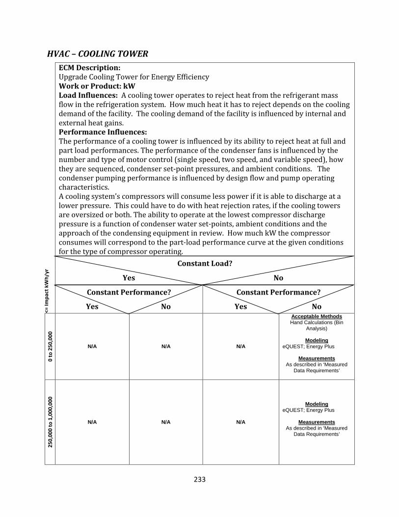
233

HVAC – COOLING TOWER

ECM Description: Upgrade Cooling Tower for Energy Efficiency Work or Product: kW Load Influences: A cooling tower operates to reject heat from the refrigerant mass flow in the refrigeration system. How much heat it has to reject depends on the cooling demand of the facility. The cooling demand of the facility is influenced by internal and external heat gains. Performance Influences: The performance of a cooling tower is influenced by its ability to reject heat at full and part load performances. The performance of the condenser fans is influenced by the number and type of motor control (single speed, two speed, and variable speed), how they are sequenced, condenser set-point pressures, and ambient conditions. The condenser pumping performance is influenced by design flow and pump operating characteristics. A cooling system’s compressors will consume less power if it is able to discharge at a lower pressure. This could have to do with heat rejection rates, if the cooling towers are oversized or both. The ability to operate at the lowest compressor discharge pressure is a function of condenser water set-points, ambient conditions and the approach of the condensing equipment in review. How much kW the compressor consumes will correspond to the part-load performance curve at the given conditions for the type of compressor operating.

<= Im

pact

kW

h/yr

Constant Load?

Yes No


Yes No Yes No

0 to

250

,000

N/A N/A

N/A

Acceptable Methods Hand Calculations (Bin

Analysis)

Modeling eQUEST; Energy Plus

Measurements As described in ‘Measured

Data Requirements’

250,

000

to 1

,000

,000

N/A N/A N/A




234

> 1,

000,

.000

0

N/A N/A N/A Not Typical


The energy savings with upgrading a cooling tower can be associated with the cooling compressors, condenser pumps, and cooling tower fans. For this reason, pre and post operating conditions and specifications needs to be acquired.

For the compressors, this would include refrigerant used, type and quantity of compressors, how they are sequenced, capacity, and temperature set-points. For cooling towers, nameplate, data, the number of condenser fans, if they are equipped with single speed, 2 speed motors or variable speed drives, and how they are staged. Condenser pump nameplate and flow requirements are required information as well as if there is any additional equipment (i.e. spray pump motor for closed loop cooling towers).

Attention should be paid to if the facility is implementing chilled water or condenser water reset strategies. These factors influence the compression ratio and condenser fan requirements at different ambient conditions.

Other information that should be collected is if the facility implements water or air-side economizer strategies. The operating hours of the system should also be discussed with the plant engineers. When applicable, attain process flow diagrams of the affected system.


The IOUs prefer that the level of sophistication for estimating savings should be higher for more complex EEM projects and/or EEMs that result in higher savings impact.

Given the overall end use consumption of the central plant, to generate energy savings greater than 250,000 kWh would have to include multiple sites or a very large facility. The largest savings associated with upgrading the cooling tower would likely have to do with reduced compressor discharge pressures (oversized cooling tower). Utilizing CEUS for IOU Zones Energy-Use Indices for All Commercial spaces, cooling equipment is estimated to consume 3.49 kWh/ft^2/year. Considering a 500,000 ft^2 facility, the cooling load consumption is 1,750,000 kWh. The rule of thumb for compressor discharge reduction is 1-1.5% energy savings off the compressor load for each degree condenser reduction. Assume that the compressor load is half the cooling load consumption and that the facility on average is able to drop the condensing temperature by 15 degrees (85 deg Condensing to 70 deg Condensing), liberally

235

speaking, installing evaporative condenser could save approximately 200,000 kWh/year for this site.

Although, the associated potential for this measure is deemed low by Utility Standards, spot measurements and monitoring is a useful tool to estimate the energy savings and should be applied as necessary. The following data requirements are guidelines in estimating and validating the energy savings associated with this measure.

Baseline Scenario

Monitor two weeks of data of outside air temperature, wet-bulb, chiller and condenser amperage. If possible, it is preferred that direct measurements of power and usage be obtained over calculating its proxy using measured amperage data. Chiller tons would also be beneficial in the analysis. Spot measurements on condenser pumps are also an important piece of information. Create a regression and estimate proposed consumption using a bin methodology.

Proposed Scenario

Monitor two weeks of data of outside air temperature, wet-bulb, chiller and condenser amperage. If possible, it is preferred that direct measurements of power and usage be obtained over calculating its proxy using measured amperage data. Chiller tons would also be beneficial in the analysis. Spot measurements on condenser pumps are also an important piece of information. Create a regression and estimate proposed consumption using a bin methodology.


Changes from baseline to post-installation production would occur if the facility increases its cooling requirements (i.e. more tenants, data servers, space functionality etc.). This should be identified in the pre-installation inspection and if this is the case, the anticipated loads needs to be assessed and savings adjusted accordingly.


In order for a project to be eligible for the Statewide Customized Offering, any existing equipment required to establish the project baseline must be operating and available for inspection.

If the facility is eligible as a new load project, the estimated new load profile should be applied to estimate the potential savings.

236


Operating Hours

The cooling plant will operate if there is a need for cooling. Schedules and economizer operation should be considered.


If engineering specification is not available an approach of 15 degrees from the wet-bulb is considered reasonable.




The following formulas are useful in estimating the energy savings associated with implementing evaporative condensers:

Measured Data

Motor kW = (1.73 X Volts X Amps X Power Factor)/1000

Pump and Fan Equations

Pump kW = (Head X Flow X Specific Gravity)/ (3960 X Pump Efficiency X Motor Efficiency)*0.7457

Fan kW = (Static Pressure X Flow X Specific Gravity)/ (6356 X Fan Efficiency X Motor Efficiency)*0.7457

237

Affinity Laws for Pumps

Energy usage of the baseline and proposed cases are determined by utilizing the affinity laws. Energy savings are then obtained by taking the difference between the two cases.

𝑔𝑝𝑚1

𝑔𝑝𝑚2 =𝑟𝑝𝑚1

𝑟𝑝𝑚2

where:

gpm = gallons per minute

rpm = revolution per minute

𝑑𝑝1𝑑𝑝2

= �𝑟𝑝𝑚1

𝑟𝑝𝑚2�2

where:

dp = head or pressure

𝑘𝑊1

𝑘𝑊2 = �

𝑔𝑝𝑚1

𝑔𝑝𝑚2�𝑛

where:

kW = pump power





Air/Water Loop is:



Open


238



20% of Less

Greater than 20%, Less than 50%

Greater than 50%, Less than 80%

80% or More



2.4








Closed Systems




Systems




Open Systems



239

Variable Geometry


Examples:









240

HVAC – COMPRESSOR RETROFIT (AC-18574)

EEM Description: Replacement of OEM compressor on existing chiller or DX systems with one or more frictionless variable speed compressors. Energy savings are realized by reduced friction losses in compressor, improved head pressure control and optimized refrigerant flow versus load. Work or Product: Tons of cooling Load Influences: Internal building loads, infiltration and weather Performance Influences: Weather, compressor staging (for multiple units), Condenser Cooling Water (CCW) approach, Inlet Guide Vane (IGV) operation, Electronic Expansion Valve (EXV) operation, CCW temp reset and proper commissioning of equipment.

<= Im

pact

kW

h/yr

Constant Load?

Yes No


Yes No Yes No

0 to

250

,000




Measurements

Short Duration (seven days) Power Consumption &

Cooling Load

250,

000

to 1

,000

,000




Measurements

Short Duration (fourteen days) Power Consumption &

Cooling Load

> 1,

000,

.000

0




Measurements

Extended Duration (one month, although one month

in summer and another month in winter is preferred)

Power Consumption & Cooling Load

241


• Obtain performance curve from the manufacturer tech sheet for the existing DX system or chiller.

• Obtain building envelope, equipment specification and schedule of facility operation from the audit, building drawing, O&M manual and facilities personnel.

• Obtain the basis for the submitted chiller/DX retrofit unit full load efficiency from the manufacture (i.e. at ARI conditions, field data, etc.).




Measurements will be required to establish the post-installation operation and to verify savings after the measure is completed. The measured data will be for a period of seven contiguous days at intervals not greater than 15 minutes (averaged) for total chiller/DX system including:

• Cooling load (Tons) on the chiller/DX coil;

• Condenser cooling water temperature, dry bulb (air cooled) and wet bulb (water and evaporative cooled) temperatures;

• Turbocor compressor and condenser fan (kW), saturated suction and saturated condensing temperatures, suction, and discharge temperatures & pressures.


The energy savings are calculated based on the monitored post-installation measurements.

Baseline Considerations One must first determine if the measure is eligible for early retirement (RET). If the measure does not qualify for early retirement (RET), then a single baseline is determined and must use the forecasted equipment load and an appropriate minimum efficiency standard to establish baseline performance. An acceptable minimum efficiency standard must be a government minimum efficiency standard or, if a minimum standard efficiency is not available, the current industry practice. If early retirement does apply, then two separate baselines must be determined. The first baseline shall be determined using the pre-existing equipment

242

efficiencies. The second baseline shall be determined using forecasted equipment load and an appropriate minimum efficiency.

Operating Hours

The operating hours are based on the scheduled equipment runs and shall be provided by customer facilities personnel. If operating hours vary depending on season, the customer must submit supporting documentation to verify seasonal operating hours.


When engineering calculations are performed, all assumptions made by the engineer and equations used in the calculations must be well documented. The assumptions regarding the building envelope and equipment specification need to be substantiated by the building operator and/or equipment manufacture. Any assumptions that are made in modeling of the chiller/DX units using eQuest/ IDSM Online Application Tool need to be substantiated as well.


As part of the IR review process, the Turbocor compressor retrofit installer shall provide the start-up sheet/commissioning report and customer installation completion report that is typically prepared by Turbocor installers. This installation completion report must contain the following information:

1. Description of remaining components from the original chiller/DX system (i.e. condenser, expansion valve type, receiving tanks and evaporator) and their conditions.

2. Provide documentation to substantiate the implementation of floating head pressure and condenser cooling water temperature reset controls.

3. Explanation, if present, of any system optimization methodology (full control or Hartman loop) that may have been implemented during installation of chiller or DX system.

4. Confirm if the refrigeration piping system is clean and free of all debris. Note any unusual piping section that may cause higher than normal pressure drop.

5. Description of oil evacuation procedures implemented. Note if a suction line accumulator was temporarily installed in front of the Turbocor compressor.

6. Note if the existing equipment, i.e. condenser and evaporator are relatively oil free (<3%) using information provided by the Turbocor monitor BMCC program.

243

7. Note if a suction line accumulator has been temporarily installed in front of the Turbocor compressor or not.

8. Compressor retrofits size relative to the baseline unit (i.e. 2-120 ton replacing 1-200 ton, etc.).

9. Compressor staging strategy description (for multiple compressors) and whether the retrofitted compressors are expected to operate in a mostly part-load condition.

10. Verify if each evaporator has its own independent EXV and a common suction temperature or pressure sensor.

11. Confirm the cooling tower capacity. If the cooling tower is shared what are the sizes of the other chillers.

12. Note if the inter-stage economizer between the two stages of compressor is operating.


For pre-installation energy savings estimation:

If this is a compressor retrofit for a DX system then:

1. Do not obtain savings directly from eQuest or IDSM Online Application Tool. 2. Obtain building hourly cooling load and hours the equipment operates from eQuest

and performs spreadsheet calculations to obtain %Capacity of DX system (hourly load/full load).

3. Title 24 minimum efficiencies are used for the baseline reciprocating/screw compressors kW/ton at full load.

4. Baseline compressor performance curves are the eQuest packaged DX unit curve and, for proposed, the OEM’s frictionless compressor DX unit published curves at ARI conditions.

If this is a compressor retrofit for a chiller system then:

1. Use eQuest/ IDSM Online Application Tool to predict the energy savings due to retrofitting frictionless compressor chiller.

2. Provide the basis for the submitted chiller retrofit unit full load kW/ton efficiency used in the model.

For post-installation energy savings estimation:

If this is a compressor retrofit for a DX system then:

244

1. Collect seven days of electric power and cooling load data (DX coil air flow measurement required).

2. Compare collected performance (kW/Ton) versus pct rated capacity against the OEM’s frictionless compressor published performance curve to confirm that unit is operating correctly. (spreadsheet template available)

3. If the performance difference is more than ±10%, diagnose installation problems and if necessary adjust OEM’s frictionless compressor performance curve to best fit collected data and re-run the spreadsheet calculations described above.

If this is a compressor retrofit for a chiller system then:

1. Collect seven days of electric power and cooling load data (Chilled water GPM required).

2. Compare collected performance (kW/Ton) versus pct rated capacity against the frictionless compressor chiller published performance curve to confirm that unit is operating correctly. (spreadsheet template available)

3. If the performance difference is more than ±10%, diagnose installation problems and if necessary adjust OEM’s frictionless compressor performance curve to best fit collected data and re-run eQuest/ IDSM Online Application Tool.


245

HVAC – CONDENSER

ECM Description: Replace air cooled condenser with evaporative condensers. Work or Product: Tons of cooling. Load Influences: Mechanical cooling is influenced by the cooling demand of the facility. Direct Expansion Air-Cooled and Evaporative Cooled condenser’s load is influenced by chiller load, condenser set-point and ambient conditions. Performance Influences: The energy savings associated with replacing an air cooled condenser with an evaporative condenser is largely to do with the air conditioning system being able to operate at a lower compressor discharge pressure. The ability to operate at the lowest compressor discharge pressure is a function of ambient conditions and the approach of the condensing equipment in review. How much kW the compressor consumes will correspond to the part-load performance curve at the given conditions for the type of compressor operating. The condensers operate to reject heat from the refrigerant mass flow from the compressors. The performance of the condenser fans is influenced by the number and type of motor control (single speed, two speed, and variable speed), how they are sequenced, condenser set-point pressures, and ambient conditions.

<= Im

pact

kW

h/yr

Constant Load?

Yes No


Yes No Yes No

0 to

250

,000

N/A N/A

N/A


Analysis) Modeling

eQUEST; Energy Plus Measurements

As described in ‘Measured Data Requirements’

250,

000

to 1

,000

,000

N/A N/A N/A




246

> 1,

000,

.000

0

N/A N/A N/A Not Typical


The energy savings associated with replacing an air cooled condenser with an evaporative condenser is largely to do with the air conditioning system being able to operate at lower compressor discharge pressures. For this reason nameplate information and specifications needs to be collected to assess the performance of the compressors. This includes refrigerant used, type and quantity of compressors, how they are sequences, capacity, and temperature set-points.

Evaporator condensers are different in comparison to air cooled condensers. Where air-cooled condensers may just have a series of condenser fans, evaporative condensers are equipped with additional equipment like a spray pump and utilize water which has a better heat transfer coefficient then air. These two pieces of equipment have different performance curves and to collect nameplate data on the number of condenser fans, if they are equipped with single speed, 2 speed motors or variable speed drives, and how they are staged.

Manufacturer’s specifications on the performance of the existing compressors, air-cooled condenser and proposed evaporative condenser should also be collected to better understand capacity and plant performance.

Economizer operation is an important consideration as well as it will impact the total load the cooling plant will need to generate. The operating hours of the system should also be discussed with the plant engineers. When applicable, attain process flow diagrams of the affected system.



Given the overall end use consumption of the central plant, to generate energy savings greater than 250,000 kWh would have to include multiple sites or a very large facility. And it is reasonable to assume that most facilities greater the 500,000 square feet of conditioned space would implement water cooled chillers in their design. Utilizing CEUS for IOU Zones Energy-Use Indices for All Commercial spaces, cooling equipment is estimated to consume 3.49 kWh/ft^2/year. Considering a 500,000 ft^2 facility, the cooling load consumption is 1,750,000

247

kWh. The rule of thumb for compressor discharge reduction is 1-1.5% energy savings off the compressor load for each degree condenser reduction. Assume that the compressor load is half the cooling load consumption and that the facility on average is able to drop the condensing temperature by 15 degrees (85 deg Condensing to 70 deg Condensing), liberally speaking, installing evaporative condenser could save approximately 200,000 kWh/year for this site.


Baseline Scenario

Monitor two weeks of data of outside air temperature, wet-bulb, chiller and condenser amperage. If possible, it is preferred that direct measurements of power and usage be obtained over calculating its proxy using measured amperage data. Chiller tons would also be beneficial in the analysis. Create a regression and estimate proposed consumption using a bin methodology.

Proposed Scenario – Installation of VFD’s

Monitor two weeks of data of outside air temperature, wet-bulb, chiller and condenser amperage. If possible, it is preferred that direct measurements of power and usage be obtained over calculating its proxy using measured amperage data. Chiller tons would also be beneficial in the analysis. Create a regression and estimate proposed consumption using a bin methodology.





248



Operating Hours

The air-cooled or evaporative cooled condenser will operate if there is a need for mechanical cooling (i.e. chiller). Schedules and economizer operation should be considered.


If engineering specification is not available for air-cooled condensers, an approach of 15 degrees from the dry bulb is considered reasonable. If engineering specification is not available for the evaporative cooled condenser, an approach of 15 degrees from the wet bulb is considered reasonable.




The following formulas are useful in estimating the energy savings associated with implementing evaporative condensers:

Measured Data

Motor kW = (1.73 X Volts X Amps X Power Factor)/1000

Pump Equations

249

Pump kW = (Head X Flow X Specific Gravity)/ (3960 X Pump Efficiency X Motor Efficiency) X 0.746

Chiller Load

Chiller Load (Tons) = 500 X Gallons/Minute X (Chilled Water Return Temperature – Chilled Water Supply Temperature)/12,000

Total Heat Rejection (THR)

THR (Btuh) = [Compressor Heat (Btuh) + Evaporator Heat (Btuh)] X Condenser Capacity Conversion Factor

Open Type Compressors: Compressor Heat (Btuh) = 2545 X Compressor BHP

Hermetic Compressors: Compressor Heat (Btuh) = Compressor kW X 3413

Evaporator Heat (Btuh) = Load (Tons) X 12,000

Part Load Evaporative Condenser Equation

Capacity Actual = Capacity Rated X (Fan Speed Actual/Fan Speed Rated) ^ (0.76)

Affinity Laws for Fans


𝑐𝑓𝑚1

𝑐𝑓𝑚2 =𝑟𝑝𝑚1

𝑟𝑝𝑚2

where:

cpm = cubic feet per minute


𝑑𝑝1𝑑𝑝2

= �𝑟𝑝𝑚1

𝑟𝑝𝑚2�2

where:


𝑘𝑊1

𝑘𝑊2 = �

𝑐𝑓𝑚1

𝑐𝑓𝑚2�𝑛

250

where:

kW = pump power





Air/Water Loop is:



Open




20% of Less


50%


80% 80% or More



2.4



251






Closed Systems




Systems




Open Systems



Variable Geometry


Examples:







252



253

HVAC – SYSTEMS VARIABLE REFRIGERANT FLOW (AC-46584)

EEM Description: Replacement of existing AC equipment with VRF systems result in energy efficiency savings in comparison to chilled water and DX ducted systems. Existing typical duct losses in the range of 10% to 20% of total supply airflow are eliminated with VRF systems. Energy Savings: are realized in VRF systems because the better match individual building load zones with more precision or exactness. This is due to its wide capacity modulation characteristic found in their condensing unit design due to the use of variable speed compressors and sophisticated electronic controls. Work or Product: Tons of Cooling and Heating Load Influences: Weather, loads, equipment schedule, and building envelope parameters, infiltration, internal heat gains, occupancy and miscellaneous loads. Performance Influences: Weather, and misapplication of VRF system.

<= Im

pact

kW

h/yr

Constant Load?

Yes No


Yes No Yes No

0 to

250

,000



analysis calculations EnergyPro

eQuest -WIP

Measurements Short duration on consuming energy system components

(Duration will depend on variability in performance and

load – 1 week) units

250,

000

to 1

,000

,000




eQuest -WIP

Measurements Extended duration on

consuming energy system components


load – 2- 4 weeks)

254

> 1,

000,

.000

0




eQuest -WIP

Measurements Extended duration on

consuming energy system components


load – 4 week)


Obtain VRF system engineering product data specifications from customer/project sponsor. If product data is not available from either one of them, then please contact the original equipment manufacturer. When applicable, attain process flow diagrams of the affected system.

VRF product data specifications should contain the following information:

• Cooling Capacity & Heating Capacity: BTUH

• Power input (kW): compressor(s) + outdoor fan motor(s)

• Outdoor air temperature

• Compressor(s) specifications

• Indoor & outdoor fan motor(s) specifications





255



For retrofit of existing/systems with different capacity equipment than the baseline or post-installation production levels are different (i.e. the equipment load is higher or lower), the annual energy savings will be calculated assuming the post-installation production load or load system. The general equation for calculating savings with changes in production is:

Eligible Energy Savings (kWh/yr) = (Baseline Efficiency – Proposed Efficiency) x Proposed Production rate or Load x Proposed Operating Hours.


In order for a project to be eligible for the Statewide Customized Offering, any existing equipment required to establish the project baseline must be operating and available for inspection. Moreover, the equipment must be running and in good condition at the time of the inspection.


Operating Hours



Same operating hours of building schedule, equipment schedule and building load profile.

256


Building design construction and piping distance application from condensing unit(s) to fan coil(s) are critical and special requirement to consider due to oil return to compressor(s).


Published ARI directory or company product engineering data for existing equipment at full load and part load capacity and efficiency should be used when comparing to a new proposed system if available. If not available, installation of data loggers on pertinent equipment are required to establish the baseline energy consumption (kWh) and energy demand (kW). Then develop a regression analysis based on logged and recorded data in conjunction with corresponding climate zone weather bin temperature data. The same approach could be used for the installation review phase to correct and verify the proposed energy savings.

257

HVAC – CONTROLS CAV to VAV CONVERSIONS (AC-68030)

EEM Description: The air-side portion of an HVAC system is modified to meet changing cooling load requirements by adjusting the amount of cool air that is supplied to a conditioned space. The temperature of the cool air is adjusted in the baseline condition to meet load demand. Work or Product: BTUH or tons of cooling Load Parameters: Building envelope attributes, ambient air conditions, building occupancy Performance Influences: Ambient air conditions (condenser water), system load, airflow requirements (supply fans at post installation)

<= Im

pact

kW

h/yr

Constant Load?

Yes No


Yes No Yes No

0 to

250

,000

Not Typical


Acceptable Methods eQUEST v 3.63 or 3.64 –

Whole Site/Building EEM or Parametric Runs

Measurements

None

250,

000

to 1

,000

,000


Acceptable Methods

eQUEST v 3.63 or 3.64 – Whole Site/Building EEM or

Parametric Runs

Measurements None

> 1,

000,

.000

0

Not Typical


Acceptable Methods

eQUEST v 3.63 or 3.64 – Whole Site/Building EEM or

Parametric Runs

Measurements Fan power, compressor

power, and cooling load of the system

258


A manufacturer’s specification sheet or documentation should be obtained to verify the energy performance profile of the refrigeration system. If a project is submitted without specification sheets, then the minimum standard (Title 24) may be appropriate for the given system size and type. Similarly, manufacturer’s information regarding the fan size and capacity should be obtained if this information is not available from a system nameplate. Motor information should be available during site inspections. When applicable, process flow diagrams of the affected system should be attained.

A contractor’s scope of work or similar documentation can be used to verify the applicable equipment has been removed and appropriate equipment installed that constitute this measure.


Measured data is not typically required for smaller projects due to the fact that system performance is largely dependent on annual weather patterns. However, short term monitoring may be required to verify the operating hours of the facility.

For applications larger than 1,000,000 kWh, fan power, compressor power, and cooling load of the system should be measured to verify system performance. The monitoring period should be no less than two weeks and include all operating modes of the equipment. This data monitoring should be conducted in both the pre and post installation cases to verify the energy model.


The work product (BTUH or Tons of cooling) of the system is reduced through the implementation of a variable volume (VAV) air-side HVAC system. The required amount of cooling to meet the building load is still provided in the post-installation condition, however some of the excess cooling provided in the baseline case would be eliminated. This is accomplished by reducing the amount of air volume that is seen by the cooling coils.

If the cooling requirements of the facility are changed from the baseline condition – potentially due to a change in operating hours or occupancy -- then the latest operating schedule is to be used in the savings calculations.


In order for a project to be eligible for the Statewide Customized Offering, any existing equipment required to establish the project baseline must be operating and available for

259

inspection. The proposed equipment required for the upgrade (VAV boxes, dampers, duct work, etc) cannot be installed or on site in the baseline condition.


Operating Hours

Baseline system operating hours should, at minimum be estimated in accordance with the existing operating hours of the facility. When not supportable with available data, DEER values by building type should be used as proxies. When appropriate, it is recommended that baseline system operating hours be calculated based on short term monitoring. For fixed speed baselines, motor loggers (ON/OFF) should be installed to determine system operating hours.

The proposed operating hours should be determined through an accepted modeling program.


Assumptions regarding facility space type can be made to match that of the DEER Model building prototypes. Efficiency of the refrigeration equipment and fan-motor system may be assumed in lieu of available specification sheets.

eQUEST system defaults are acceptable for most inputs with the exception of those relating specifically to that of the measure involved and that of the air-side system. If the inputs unrelated to the specific measure in the building energy simulation have been customized, then the inputs must be supported with applicable documentation.


Though the measure is designed to minimize the amount of airflow while still meeting the internal cooling load of the building, there are minimum ventilation requirements that impact this reduction. These requirements vary depending on the facility type and other factors. For

260

more information, please refer to the recommended ventilation rates contained in ASHRAE standard 62.1.


The energy savings for constant to variable air volume conversion projects should be calculated using the building energy simulation software tool, eQUEST (v3.63 or v3.64). The energy model and subsequent savings can be calculated using the Whole Site/Building EEM (Energy Efficiency Measure) or through the use of Parametric Runs.

This tool should be used due to the fact that it utilized hourly annual weather data specific to a California Climate Zone. This information, along with the building characteristics such as building envelope details and occupancy profiles, is used to determine hourly cooling load profiles on an annual basis. This cooling demand profile is then applied to the pre and post installation air-side HVAC system to determine annual energy consumption of pre and post installation scenarios.

The appropriateness of the model can be verified through hourly reports generated by the simulation tool. The airflow should be constant in the baseline and varying in the replacement scenario.

DEER Peak Demand savings are also calculated by this tool. The kW consumption for the applicable CPU defined peak demand period is to be extracted from hourly reports.

261

HVAC – CONTROLS FAN STATIC PRESSURE RESET (AC-96957)

EEM Description: The static pressure set point controlling the supply fans is allowed to adjust based on the position of the airflow dampers in each zone. Work or Product: BTUH or tons of cooling Load Parameters: Building envelope attributes, ambient air conditions, building occupancy Performance Influences: Ambient air conditions (condenser water), system load, static pressure requirements (supply fans at post installation), fan control type

<= Im

pact

kW

h/yr

Constant Load?

Yes No


Yes No Yes No

0 to

250

,000

Not Typical


Acceptable Methods FanSystemCalc v.2.0

(eQUEST v 3.63 or 3.64)

Measurements - Spot pressure

measurements of duct and fan static pressure

250,

000

to 1

,000

,000



(eQUEST v 3.63 or 3.64)



- 1 week of measurements including fan power and

static pressure in the duct

> 1,

000,

.000

0

Not Typical



(eQUEST v 3.63 or 3.64)



- 2 weeks of measurements including fan power and

static pressure in the duct

262


Drawings or relevant documentation should be obtained to verify the fan conditions at peak efficiency. This information includes fan speed, air flow, static pressure, and brake HP. It may be possible to confirm this information from a generic fan curve for a similar fan type and size. The system design air flow may be obtained from design drawings. Fan motor nameplate information should be available during site inspections from the motor nameplate. When applicable, process flow diagrams of the affected system should be attained.

Drawings or mechanical schedules depicting the new sequence of operations should be provided to confirm the pressure reset schedule in the replacement scenario.


Spot measurements are required at the static pressure sensor and static pressure at the supply fan with all system dampers open. These measurements are required for all projects. If these measurements are unable to be obtained, then the information may be obtained through calculations based on design data.

For applications with savings estimates larger than 250,000 kWh, fan power and duct static pressure should be monitored for a period of no less than one (1) week to verify system performance. It is recommended that this period be increased to two (2) weeks for savings projects larger than 1,000,000 kWh. This data monitoring should be conducted in both the pre and post installation cases to verify the energy model.

This information may be available from the control system computer in the post installation case.


The work product for this measure is BTUH or tons of cooling. The required amount of this product does not change through the implementation of static pressure reset control. The amount of fan power required to supply the airflow to meet the building cooling demand is reduced through the implementation of this measure.

If the cooling requirements of the facility are changed from the baseline condition – potentially due to a change in operating hours or occupancy -- then the latest operating schedule is to be used in the savings calculations.

263


In order for a project to be eligible for the Statewide Customized Offering, any existing equipment required to establish the project baseline must be operating and available for inspection. The proposed equipment required for the upgrade includes a direct digital control system (DDC) with the capability to reset the pressure set point controlling the supply fans. If this capability exists in the baseline condition of the system, then the measure is ineligible for savings.

The baseline fan system should have an existing control system (such as air dampers, guide vanes, or variable speed drive).


Operating Hours

The operating hours are developed by a building simulation tool (eQUEST) that is used to develop the CFM profile required from the existing air-side HVAC system to meet the annual cooling load of the building or facility. The annual operating hours of the fan are allocated into CFM bins based on outside air temperature. Though eQUEST calculates the system baseline operating hours, it requires the general operating hours of the facility or cooled areas as inputs. These inputs should, at minimum be estimated in accordance with the existing operating hours of the facility. When not supportable with available data, DEER values by building type should be used as proxies. When appropriate, it is recommended that baseline system operating hours be calculated based on short term monitoring. For fixed speed baseline, motor loggers (ON/OFF) should be installed on the applicable equipment to determine facility operating hours.

System operating hours are not expected to be affected by this measure unless there is a change in the production of the facility. If there is a change in facility operation, then the system operating hours should be re-calculated.


It is assumed that the cooling load and subsequently, the air flow required from the air-side HVAC system, are dependent on ambient air temperature.

264

eQUEST system defaults are acceptable for most inputs with the exception of those relating specifically that of the air-side system. If the inputs unrelated to the specific measure in the building energy simulation have been customized, then the inputs must be supported with applicable documentation. Assumptions regarding facility space type can be made to match that of the DEER Model building prototypes. In some cases, efficiency of the refrigeration equipment and fan-motor system may be assumed in lieu of available specification sheets.

The replacement air side system is assumed to have full direct digital control (DDC) and feedback on VAV box damper position.


The FansystemCalc 2.0 modeling tool assumes an AHU serving a single zone. Therefore, it is critical that the zone modeled in the tool is the critical zone of the facility, meaning that it requires the greatest supply air pressure.

Additionally, the calculation tool does not account for return fan energy.

Though the measure is designed to minimize the amount of work done by the supply fans while still meeting the internal cooling load of the building, there are minimum ventilation requirements that impact this reduction. These requirements vary depending on the facility type and other factors. For more information, please refer to the recommended ventilation rates contained in ASHRAE standard 62.1.


The energy savings calculations are conducted in two stages with separate tools. First, the annual CFM profile is estimated using building energy simulation software. This should be done using eQUEST (v3.63 or v3.64) with the appropriate building type and mechanical equipment.

This tool should be used due to the fact that it utilized hourly annual weather data specific to a California Climate Zone. This information, along with the building characteristics such as envelope details and occupancy profiles, is used to determine hourly cooling load profiles on an annual basis. This cooling demand profile is then applied to the existing air-side HVAC system to determine annual energy consumption. For this measure, only the calculated CFM profile to meet the cooling load is needed. This information can be retrieved from hourly reports generated by eQUEST and then allocated into flow bins based on hourly temperature.

The FanSystemCalc 2.0 is then used develop the energy savings estimate using the static pressure set point value at the baseline. The tool utilizes the CFM flow bin information with the fan system characteristics to estimate the energy use at the measured static pressure and performs iterations to calculate the required fan speed and duct pressure for each flow bin.

265

The input efficiencies are projected to a fan curve that is used along with standard motor and VFD efficiencies to calculate the fan kW and kWh at each bin. The calculations are adjusted for the proposed condition by utilizing a pressure set point reset schedule input by the user.

Please see the Calculation Methodology of the FanSystemCalc 2.0 tool for additional information.

266

HVAC– CONTROLS HOT AND COLD DECK RESET (AC-87564)

EEM Description: The controls to the air-side portion of an HVAC system are modified to meet changing cooling load requirements by adjusting the temperature of cooling coil to adequately cool the zone with the highest temperature. The controls work in the opposite manner for hot deck reset control. Work or Product: BTUH or tons (cooling) or MBTU (heating) Load Parameters: Building envelope attributes, ambient air conditions, building occupancy Performance Influences: Ambient air conditions (condenser water), system load

<= Im

pact

kW

h/yr

Constant Load?

Yes No


Yes No Yes No

0 to

250

,000

Not Typical



Deck Reset EEM

Measurements None

250,

000

to 1

,000

,000



Deck Reset EEM

Measurements 1 week of measurements

including compressor power and cooling load

> 1,

000,

.000

0

Not Typical


Acceptable Methods

eQUEST v 3.63 or 3.64 – Deck Reset EEM

Measurements 2-3 weeks of measurements including compressor power

and cooling load

267


A manufacturer’s specification sheet or documentation should be obtained to verify the energy performance profile of the refrigeration system. If a project is submitted without specification sheets, then the minimum standard (Title 24) may be appropriate for the given system size and type. Similarly, manufacturer’s information regarding the coil size and capacity should be obtained if this information is not available from a system nameplate. When applicable, process flow diagrams of the affected system should be attained.

Drawings or mechanical schedules depicting the supply air set point in the baseline scenario. Schedules containing the new sequence of operations should also be provided to confirm the air reset schedule in the replacement scenario.


Measured data is not typically required due to the fact that system performance is largely dependent on annual weather patterns. However, short term monitoring may be required to verify the operating hours of the facility.

For applications with savings estimates larger than 250,000 kWh, compressor power and cooling load should be monitored for a period of no less than one (1) week to verify system performance. The monitoring period should include all operating modes of the equipment. For applications larger than 1,000,000 kWh, this information should be measured for a period of no less than two weeks.

This data monitoring should be conducted in both the pre and post installation cases to verify the energy model. This information may be available from the control system computer in the post installation case.


The work product for this measure is BTUH or tons of cooling. The required amount of this product does not change through the implementation of hot and cold deck reset control. However, some of the excess cooling provided in the baseline case would be eliminated. This is accomplished by increasing the set point temperature of the supply air (cooling case) while still meeting the cooling demand of the highest temperature zone. The situation is reversed for the heating case.

If the heating and/or cooling requirements of the facility are changed from the baseline condition – potentially due to a change in operating hours or occupancy -- then the latest operating schedule is to be used in the savings calculations.

268


In order for a project to be eligible for the Statewide Customized Offering, any existing equipment required to establish the project baseline must be operating and available for inspection. The proposed equipment required for the upgrade includes a direct digital control system (DDC) with the capability to reset the supply air temperature set point controlling the operation of the refrigeration or heating system. If this capability exists in the baseline condition of the system, then the measure is ineligible for savings.

This energy savings measure is typically implemented on constant volume air side systems. Though energy savings can be realized on variable volume systems, it should be noted that an energy trade off situation may result. This is due to the fact that by reducing the required supply air temperature, compressor work is reduced; however the amount of required system air volume is increased which thereby increases fan use.


Operating Hours

The operating hours are developed by a building simulation tool (eQUEST) that is used to develop the typical annual cooling demand required to be met by the existing refrigeration system. Though eQUEST calculates the system baseline operating hours, it requires the general operating hours of the facility or cooled areas as inputs. These inputs should, at minimum be estimated in accordance with the existing operating hours of the facility. When not supportable with available data, DEER values by building type should be used as proxies. When appropriate, it is recommended that baseline system operating hours be calculated based on short term monitoring. Motor loggers (ON/OFF) should be installed on the applicable equipment to determine facility operating hours.


Assumptions regarding facility space type can be made to match that of the DEER Model building prototypes. In some cases, efficiency of the refrigeration equipment may be assumed in lieu of available specification sheets.

eQUEST system defaults are acceptable for most inputs with the exception of those relating specifically to that of the measure involved (refrigeration compressor and applicable auxiliary equipment). If the inputs unrelated to the specific measure in the building energy simulation

269

have been customized, then the inputs must be supported with applicable documentation. The baseline cooling supply air temperature is typically set at 55 deg. It is reasonable to assume this value in lieu of available schedules or drawings for projects under 250,000 kWh.

The replacement air side system is assumed to have full direct digital control (DDC) and feedback on cold and/or hot deck temperature.


It should be noted that hot deck reset measures typically result in gas savings (therms) and may not be applicable. Electric energy savings are not typically realized for hot deck reset controls unless the system utilizes resistive heating.


The energy savings for supply air (hot and cold deck) reset projects should be calculated using the building energy simulation software tool, eQUEST (v3.63 or v3.64) – Deck Reset EEM (Energy Efficiency Measure).

This tool should be used due to the fact that it utilized hourly annual weather data specific to a California Climate Zone. This information, along with the building characteristics such as building envelope details and occupancy profiles, is used to determine hourly cooling load profiles on an annual basis. This cooling demand profile is then applied to the pre and post installation supply air set point scenarios to determine annual energy savings.

The baseline supply air set point scenario utilizes a constant supply air set point value (default 55 deg) to meet the required cooling load at any given time. The proposed measure scenario sets the cold deck each hour to adequately cool the zone with the highest temperature. The situation is reversed for hot deck reset. A minimum and maximum allowable deck temperature is defined by the user.

DEER Peak Demand savings are also calculated by this tool. The kW consumption of the refrigeration equipment for the applicable CPU defined peak demand period can be extracted from hourly reports.

270

HVAC – CONTROLS (AC-45213 & AC-68796)

EEM Description: The functionality of zone thermostats is enhanced to enable the temperature set point be adjusted based on time of day, day type, as well as occupancy. Work or Product: BTUH or tons (cooling) Load Parameters: Building envelope attributes, ambient air conditions, building occupancy Performance Influences: Ambient air conditions (condenser water), system load

<= Im

pact

kW

h/yr

Constant Load?

Yes No


Yes No Yes No

0 to

250

,000

Not Typical


Acceptable Methods eQUEST (v3.63 or v3.64) –

Tstat Management EEM (Parametric Runs for Occupancy Sensors),

Engage 2008 – Thermostat Setback and/or set points, or POST – PTAC Occupancy Sensors for motels/small

hotels

Measurements None

250,

000

to 1

,000

,000


Acceptable Methods eQUEST (v3.63 or v3.64) –

Tstat Management EEM (Parametric Runs for Occupancy Sensors)

Or Engage 2008 – Thermostat Setback and/or set points

Measurements

1 week of measurements including compressor power

and cooling load

271

> 1,

000,

.000

0

Not Typical


Acceptable Methods

eQUEST (v3.63 or v3.64) – Tstat Management EEM

(Parametric Runs for Occupancy Sensors)

Or Engage 2008 – Thermostat Setback and/or set points

Measurements

2-3 weeks of measurements including compressor power

and cooling load


A manufacturer’s specification sheet or documentation should be obtained to verify the energy performance profile of the refrigeration system. If a project is submitted without specification sheets, then the minimum standard (Title 24) may be appropriate for the given system size and type. When applicable, process flow diagrams of the affected system should be attained.

Manufacturer’s specifications should be obtained to verify the programming capabilities of the baseline (if applicable) and replacement thermostats.


Measured data is not typically required for HVAC control measures due to the fact that system performance is largely dependent on annual weather patterns. However, short term monitoring may be required to verify the operating hours of the facility.

For applications with savings estimates larger than 250,000 kWh, compressor power and cooling load should be monitored for a period of no less than one (1) week to verify system performance. The monitoring period should include all operating modes of the equipment. For applications larger than 1,000,000 kWh, this information should be measured for a period of no less than two weeks.

This data monitoring should be conducted in both the pre and post installation cases to verify the energy model.


The work product for this measure is BTUH or tons of cooling. Given the same performance influences, the amount of the product is reduced through the implementation of programmable thermostats with setback capabilities due to the fact that a higher temperature is sought to be achieved (cooling scenario).

272

If the heating and/or cooling requirements of the facility are changed from the baseline condition – potentially due to a change in operating hours or occupancy -- then the latest operating schedule is to be used in the savings calculations.


In order for a project to be eligible for the Statewide Customized Offering, any existing equipment required to establish the project baseline must be operating and available for inspection. Typically this equipment is to include thermostats that are set manually with no central control. In any case, the replacement equipment must demonstrate an increase in functionality over the baseline zone thermostat controls.


Operating Hours

The operating hours are developed by a building simulation tool (eQUEST or Engage) that is used to develop the typical annual cooling demand required to be met by the existing refrigeration system. Though these simulation tools calculate system baseline operating hours, they require the general operating hours of the facility or cooled areas as inputs. These inputs should, at minimum be estimated in accordance with the existing operating hours of the facility. When not supportable with available data, DEER values by building type should be used as proxies. When appropriate, it is recommended that baseline system operating hours be calculated based on short term monitoring. Motor loggers (ON/OFF) should be installed on the applicable equipment to determine facility operating hours.


Assumptions regarding facility space type can be made to match that of the DEER Model building prototypes. In some cases, efficiency of the refrigeration equipment may be assumed in lieu of available specification sheets.

eQUEST system defaults are acceptable for most inputs with the exception of those relating specifically to that of the measure involved (refrigeration compressor and applicable auxiliary equipment). If the inputs unrelated to the specific measure in the building energy simulation have been customized, then the inputs must be supported with applicable documentation. It is reasonable to assume that on average, manual thermostat set points are 74 deg cooling and 68

273

deg heating. These values can be accepted as baseline conditions in lieu of available schedules or drawings.

For measures involving the implementation of programmable thermostat control with occupancy sensor functionality, it is reasonable for calculations to utilize occupancy rates by building type as defined by DEER. DEER assumptions are limited to the building types listed in the

DEER spreadsheet.

The replacement HVAC system is assumed to have full direct digital control (DDC) and feedback on zone temperature.


For Wireless HVAC controls/thermostats:

1. The wireless devices must be supplied with an active feedback system that provides an alarm/clear notification when the unit's battery is low and requires replacement.

2. The EUL will be the battery life in years divided by two. 3. The minimum battery life must be at least 5 years (or longer) to qualify for an incentive.

A third party test is required to verify the battery life.


The energy savings for supply air (hot and cold deck) reset projects should be calculated using building energy simulation software tools. The most appropriate tools are eQUEST (v3.63 or v3.64) – Tstat Management EEM (Energy Efficiency Measure) and Engage 2008 – Thermostat Setback and/or set points. While both tools may be appropriate in certain instances, eQUEST offers the user the ability to create a more customizable model.

These tools are appropriate due to the fact that they utilize hourly annual weather data specific to a California Climate Zone. This information, along with the building characteristics such as building envelope details and occupancy profiles, is used to determine hourly cooling load profiles on an annual basis based on the given thermostat set points defined by the user. Higher temperature set points reduce the cooling load required by the refrigeration system.

It should be noted that the listed tools do not have the capability to account for intermittent zone occupancy, meaning that unoccupied time must be scheduled regularly (for example overnight and during holidays). Energy savings calculations for measures involving the implementation of occupancy sensor functionality with programmable thermostats control should utilize parametric eQUEST runs. Parametric runs are recommended to account for the changes to the controlling cooling and heating set points throughout the course of the facility operation.

274

DEER Peak Demand savings are also calculated by this tool. The kW consumption of the refrigeration equipment for the applicable CPU defined peak demand period can be extracted from hourly reports.

The PTAC Occupancy Sensor Calculation Tool (POST) can be used to estimate the energy savings associated with projects less than 250,000 kWh involving the installation of occupancy sensors on Packaged Terminal Air Conditioning (PTAC) units. For these projects, sensors are installed in the individual motel/hotel room to detect motion or body heat and a switch is installed between the PTAC unit and power outlet. Once the switch receives a signal from the sensor, the PTAC unit is turned on or off accordingly. The tool is only applicable for PTAC units with electric resistance heating in motel or small hotel applications. Measurement and verification of savings is not required for projects of this type and size.

275

HVAC – CONTROLS VFD ON CHILLED WATER PUMP MOTOR (AC-50398)

ECM Description: Install Variable Frequency Drives to single stage chilled water pumps Work or Product: Flow or Tons of cooling Load Influences: Chilled Water Pump kW will vary based on chiller demand, which is a function of the chilled water temperature control, economizer capabilities, and cooling requirements of the building. *Note: This document provides saving estimation approaches for primary-only systems or the secondary loop of a primary-secondary loop chilled water distribution configuration. In addition, the implementation of control strategies such as pump differential pressure reset measures is not considered in the document. Performance Influences: Three Way Valves – For air handling units that are equipped with three way valves (i.e. bypass), the CHW Pump will operate at constant power. The number of chilled water pumps operating is dependent on how many CHW Pumps are present in the distribution loop and how they are commissioned to operate. Typically, there may be redundancy in pumps where a fixed number will only operate in a parallel. If there are multiple chillers and CHW Pumps, then the pumps may be initiated when the lead pump is unable to meet the load. In order to implement variable speed drives, two way valves must be installed so that the chilled water pump can sense pressure changes in the loop to vary its speed based on differential pressure. Two Way Valves – For air handling units that are equipped with two way valves (i.e. no bypass), the CHW Pump power draw will vary based on the demand at the zones. When the demand of a zone is satisfied, the two way modulating valve at the air handler will begin to close creating increased pressure in the line. As this occurs, the CHW Pump will throttle back operating at a different point on its pump curve. The number of chilled water pumps operating is dependent on how many CHW Pumps are present in the distribution loop and how they are commissioned to operate. Typically, there may be redundancy in pumps where a fixed number will only operate in parallel. If there are multiple chillers and CHW Pumps, then the pumps may be initiated when the lead pump is unable to meet the load.

<= Im

pact

kW

h/yr

Constant Load?

Yes No


Yes No Yes No

276

0 to

250

,000

N/A N/A


Analysis) DEER Database

Modeling California Commissioning

Collaborative (IDSM Online Application Tool) Pump and Fan Tool; eQUEST; Energy

Plus





Modeling

California Commissioning Collaborative (IDSM Online Application Tool) Pump and Fan Tool; eQUEST; Energy

Plus



250,

000

to 1

,000

,000

N/A N/A Not Typical Not Typical

> 1,

000,

.000

0



In considering baseline electricity consumption, the chilled water distribution system needs to be assessed. It must be determined if there are two-way, three-way valves or both. It should also be noted on how the facility engineers operate the pumps, if there is redundancy and what the operating schedules are. When applicable, process flow diagrams of the affected system should be attained.

Economizer operation is an important consideration as well as it will impact the amount of pumping required by the CHW Pumps. It is also beneficial to consider chilled water and supply air set-points in the analysis as these are variables to consider in pre and post analysis.

Pump motor and nameplate data should be obtained from the pre-field inspection in addition to an understanding of the demand and cooling loads of the facility. Pump curves are also beneficial in understanding pump performance.

277



Given the size of HVAC Chilled Water Pump Motors for space conditioning, the baseline consumption rarely would exceed 250,000 kWh. In order to achieve these values, a number of separate VFD measures may need to be included.

*DEER does not show any savings converting from a 2-way Valve to VFD’s for a chilled water pump.


Baseline Scenario – Three Way Valves

Take spot measurements of the chilled water pump to establish a baseline power draw.

Baseline Scenario – Two Way Valves

Temperature and chilled water pump consumption correlates fairly well with one another. Monitor two weeks of data of outside air temperature and amperage of chilled water pumps. If possible, it is preferred that direct measurements of power and usage be obtained over calculating its proxy using measured amperage data. Create a regression and estimate proposed consumption using a bin methodology.


Temperature and chilled water pump consumption correlates fairly well with one another. Monitor two weeks of data of outside air temperature and amperage of chilled water pumps. If possible, it is preferred that direct measurements of power and usage be obtained over calculating its proxy using measured amperage data. Create a regression and estimate proposed consumption using a bin methodology.


Changes from baseline to post-installation production would occur if the facility increases its cooling requirements (i.e. more tenants, data servers, space functionality etc.). This should be

278

identified in the pre-installation inspection and if this is the case, the anticipated loads needs to be assessed and savings adjusted accordingly.





Operating Hours

Chilled Water Pumps will operate if there is a need for mechanical cooling (i.e. chiller) for the air handlers it serves. Schedules and economizer operation should be considered.


For a three way chilled water piping configuration, it is reasonable to assume that the power draw of the chilled water pump is constant during operation. When considering a minimum pump flow, 30% speed is reasonable.



Please note 3-way to 2-way valve conversion is not eligible under the Customized Program. 2-way valves are required by code, and therefore, provide no savings for retrofit types NEW or ROB. For RET measures, savings only exist for the RUL (i.e. first baseline) period. The EUL of a valve is approximated by the life of an HVAC unit and is assumed to be 15 years, which yields a 5 year RUL according to the DEER approach (RUL = 1/3 * EUL). However, any new HVAC unit installed within the last 5 years would be held to code, and code requires 2-way valves. As

279

such, there is no eligible savings for retrofit type RET. 3-way to 2-way valve conversion is only eligible under the RCx Program.


The following formulas are useful in estimating the energy savings associated with implementing variable speed drives on CHW Pumps:

Measured Data

Pump kW = (1.73 X Volts X Amps X Power Factor)/1000

Pump Equations

Pump kW = (Head X Flow X Specific Gravity)/ (3960 X Pump Efficiency X Motor Efficiency)



𝑔𝑝𝑚1


𝑟𝑝𝑚2

where:



𝑑𝑝1𝑑𝑝2

= �𝑟𝑝𝑚1

𝑟𝑝𝑚2�2

where:


𝑘𝑊1

𝑘𝑊2 = �

𝑔𝑝𝑚1


where:

kW = pump power


280




Air/Water Loop is:



Open




20% of Less


50%


80% 80% or More



2.4




281





Closed Systems




Systems




Open Systems



Variable Geometry


Examples:









282

HVAC – CONTROLS VFD ON CONDENSER WATER PUMP MOTOR (AC-74984)

ECM Description: Install Variable Frequency Drives to single stage condenser water pumps Work or Product: Tons of Cooling Load Influences: Condenser pump kW is driven by condenser water flow requirements from the chiller. Typical configuration is each chiller has its own dedicated cooling tower and condenser water pump and the number of condenser pumps operating is dependent on the number of chillers in operation. After implementation of variable speed drives, the pump flow requirements are a function of chiller load, condenser supply temperature set-point and ambient conditions. Performance Influences: Condenser pumps operate in an open loop system and draw constant power when in operation.

<= Im

pact

kW

h/yr

Constant Load?

Yes No


Yes No Yes No

0 to

250

,000

N/A N/A


Analysis)


Measurements

Spot Measurements for baseline case to establish

base case demand.

N/A

250,

000

to 1

,000

,000

N/A N/A

Modeling

eQUEST; Energy Plus

Measurements Spot Measurements for

baseline case to establish base case demand.

N/A

> 1,

000,

.000

0

N/A N/A Not Typical N/A

283


To assess condenser pump VSD measures, the configuration and operation of the chilled water plant needs to be understood. The number of chillers and how they are sequenced will provide an understanding of how often the condenser pumps are on and will operate. It should be noted if the cooling tower and condenser pumps are dedicated to a chiller or if the condenser water has a common header. When applicable, attain process flow diagrams of the affected system.

Collect cooling tower nameplate information and gather equipment specifications. Knowing the cooling towers ability to reject heat under specific ambient conditions (delta T across the tower) is an important factor in estimating proposed consumption. It also should be noted on how the condenser water is controlled (i.e. condenser supply set-point temperature, reset strategy) and if the facility implements air or water side economizers. The condenser pump curves can also be obtained for pre-field analysis.

Spot measurements should be collected in addition to nameplate information to establish baseline kW draw as condenser pumps are generally oversized. Operating parameters such as condenser supply and return temperatures, chiller load and ambient temperatures should also be recorded.


SCE prefers that the level of sophistication for estimating savings should be higher for more complex EEM projects and/or EEMs that result in higher savings impact.

The ability for condenser pumps to reduce speed is a function of the heat rejection requirements of the operating chillers. The greater the hours the chillers operate at part-load, the greater the potential savings. The scale of the energy savings associated with condenser pump vfd’s is also a function of how often the condenser pumps are required to operate and how oversized the condenser pumps currently are.

Given the size of HVAC CW Water Pump Motors for space conditioning, the baseline consumption rarely would exceed 250,000 kWh. . In order to achieve these values, a number of separate VFD measures may need to be included. Engineering judgment should be used to determine if post monitoring verification is necessary.

Although, the associated potential for this measure is deemed low by Utility Standards, spot measurements to establish a baseline power consumption for the condenser pump is recommended over using nameplate information since condenser pumps are typically

284

oversized. Post monitoring data collection is a useful tool to validate the energy savings and should be applied as necessary. The following data requirements are guidelines in estimating and validating the energy savings associated with this measure.

Baseline Scenario

Take spot measurements of the condenser water pump to establish a baseline power draw.


To verify energy savings associated with this measure, condenser pump amperage, condenser delta T, and ambient conditions should be collected for two weeks. If possible, it is preferred that direct measurements of power and usage be obtained over calculating its proxy using measured amperage data. For further accuracy, data to estimate chiller tonnage should be collected.







Operating Hours

Condenser Pumps will operate if the chillers are in operation. Schedules and operation should be discussed with the facility engineers.

285


For baseline condenser pump operation, it is reasonable to assume that the power draw of the condenser pump is constant during operation.




The following formulas are useful in estimating the energy savings associated with implementing variable speed drives on CW Pumps:

Measured Data


Water-Side Equations

Heat Rejection Capacity (Btuh) = 500 X Gallons/Minute X (Condenser Return Temperature – Condenser Supply Temperature)

Pump Equations




𝑔𝑝𝑚1


𝑟𝑝𝑚2

where:



286

𝑑𝑝1𝑑𝑝2

= �𝑟𝑝𝑚1

𝑟𝑝𝑚2�2

where:


𝑘𝑊1

𝑘𝑊2 = �

𝑔𝑝𝑚1


where:

kW = pump power





Air/Water Loop is:



Open




20% of Less


50%


80% 80% or More


287


2.4








Closed Systems




Systems




Open Systems



Variable Geometry


Examples:



288







289

HVAC – CONTROLS VFD ON HOT WATER PUMP MOTOR (AC-69858)

ECM Description: Install Variable Frequency Drives to single stage hot water pumps Work or Product: Flow or Btu’s of heating Load Influences: Hot Water Pump kW is driven by the heating demand of the facility. However, the pump kW draw will be dependent on if the hot water distribution system is equipped with two or three way valves. *Note: This document provides saving estimation approaches for primary-only systems or the secondary loop of a primary-secondary loop hot water distribution configuration. In addition, the implementation of control strategies such as pump differential pressure reset measures is not considered in the document. Performance Influences: Three Way Valves – For air handling and reheat units that are equipped with three way valves (i.e. bypass), the HW Pump will operate at constant power. The number of hot water pumps operating is dependent on how many hot water pumps are present in the distribution loop and how they are commissioned to operate. Typically, there may be redundancy in pumps where a fixed number will only operate in a parallel. If there are multiple boilers and HW Pumps, then the pumps may be initiated when the lead pump is unable to meet the load. In order to implement variable speed drives, two way valves must be installed so that the hot water pump can sense pressure changes in the loop to vary its speed based pressure differential. Two Way Valves – For air handling and terminal reheat units that are equipped with two way valves (i.e. no bypass), the HW Pump power draw will vary based on the demand at the zones and the air handler. When the demand of a zone is satisfied, the two way modulating valve at the reheats will begin to close creating increased pressure in the line. This is the same for the heating coil at the air handler. As this occurs, the HW Pump will throttle back operating at a different point on its pump curve. The number of hot water pumps operating is dependent on how many HW Pumps are present in the distribution loop and how they are commissioned to operate. Typically, there may be redundancy in pumps where a fixed number will only operate in parallel. If there are multiple boilers and HW Pumps, then the pumps may be initiated when the lead pump is unable to meet the load.

<= Im

pact

kW

h/yr

Constant Load?

Yes No


Yes No Yes No

290

0 to

250

,000

N/A N/A



Modeling


Plus





Modeling


Plus



250,

000

to 1

,000

,000


> 1,

000,

.000

0



In considering baseline electricity consumption, the hot water distribution system needs to be assessed. It must be determined if there are two-way, three-way valves or both. It should also be noted on how the facility engineers operate the pumps, if there is redundancy and what the operating schedules are. It is also beneficial to consider hot water and supply air set-points in the analysis as these are variables to consider in pre and post analysis. When applicable, process flow diagrams of the affected system should be attained.

Pump motor and nameplate data should be obtained from the pre-field inspection in addition to an understanding of the demand and heating demands of the facility. Pump curves are also beneficial in understanding the operating performance of the pumps.



291

Given the size of HVAC Hot Water Pump Motors for space conditioning, the baseline consumption rarely would exceed 250,000 kWh. In order to achieve these values, a number of separate VFD measures may need to be included. Using DEER as a benchmark, for a hospital that operates 24/7 converting from 3-way to 2-way with VSD generates energy savings on the liberal side of around 4,000 kWh/nameplate hp (energy savings associated with an office building can be half of this value). This equates to approximately a 60 hp motor. It should also be noted that the reduction in motor heat gains may offset and cost savings associated with implementing variable speed drives.


Baseline Scenario – Three Way Valves

Take spot measurements of the hot water pump to establish a baseline power draw.

Baseline Scenario – Two Way Valves

Temperature and hot water pump consumption correlates reasonably well with one another. Monitor two weeks of data of outside air temperature and amperage of hot water pumps. If possible, it is preferred that direct measurements of power and usage be obtained over calculating its proxy using measured amperage data. Create a regression and estimate proposed consumption using a bin methodology.


Temperature and hot water pump consumption correlates reasonably well with one another. Monitor two weeks of data of outside air temperature and amperage of hot water pumps. If possible, it is preferred that direct measurements of power and usage be obtained over calculating its proxy using measured amperage data. Create a regression and estimate proposed consumption using a bin methodology.



292





Operating Hours

Hot Water Pumps will operate if there is a need for heating in the zones. Schedules and operation should be discussed with the facility engineers.


For a three way hot water piping configuration, it is reasonable to assume that the power draw of the hot water pump is constant during operation. When considering a minimum pump flow, 30% speed is reasonable.




The following formulas are useful in estimating the energy savings associated with implementing variable speed drives on HW Pumps:

Measured Data


Pump Equations

293




𝑔𝑝𝑚1


𝑟𝑝𝑚2

where:



𝑑𝑝1𝑑𝑝2

= �𝑟𝑝𝑚1

𝑟𝑝𝑚2�2

where:


𝑘𝑊1

𝑘𝑊2 = �

𝑔𝑝𝑚1


where:

kW = pump power





Air/Water Loop is:



Open

294




20% of Less


50%


80% 80% or More



2.4








Closed Systems




Systems



295


Open Systems



Variable Geometry


Examples:









296

OFFICE EQUIPMENT – COMPUTERS

EEM Description: The measure includes a data center server virtualization. Server virtualization is the consolidation of low performance physical servers into higher performance physical servers. Servers can use virtualization software to allocate hardware to virtualized servers as needed. Work or Product: Information Storing and/or Retrieving and/or Processing Load Influences: None Performance Influences: None

<= Im

pact

kW

h/yr

Constant Load

Yes No


Yes No Yes No

0 to

250

,000

Acceptable Methods Excel Sheet- Server

Virtualization

Measurements None


250,

000

to 1

,000

,000


Virtualization

Measurements Spot Measurement of Power


> 1,

000,

.000

0


Virtualization

Measurements Short Duration Power

Consumption



Obtain specification sheets for existing and proposed server equipment and UPS. The specification sheets should include power (kW) demand of equipment. Obtain basis for assumed CPU loading or references to live spreadsheets by manufacturer that allow the user to calculate kW based on the typical, average CPU load. In addition Server list should be provided as well. In most cases, the site should be able to print out a list of physical servers along with

297

the server name. A similar list should be provided in the post-install showing that the servers were removed. If custom built servers are found in the existing equipment, specifications should be provided. Specs should provide CPU type, speed, amount of RAM, number of hard drives as well as any other peripherals or expansions to the system that may affect power consumption. Network Area Storage (NAS) spec sheet would be required if one is being added.


The measured data will typically be for a period of one (1) week at intervals of 15 minutes or less and will include power (kW) of the baseline equipment and proposed equipment. Monitored data would only be required for large (Savings>1,000,000 kWh) impact projects. For a medium impact (250,000 <Savings<1,000,000 kWh) project a spot measurement of power (kW) demand would typically be sufficient due to the constant performance and load of the equipment. All energy savings measurements must be taken upstream of any UPS (even if it wasn’t replaced). The calculated energy savings shall include the UPS losses.


In some cases additional storage is needed. If a Network Area Storage (NAS) is used in the post and not the preexisting case, the power consumption for the NAS will need to be counted in the post-installation calculations.



Operating Hours

Typical operating hours are 8,760 hours per year.


To use the Excel Sheet- Server Virtualization, it is assumed the baseline and proposed equipment power demand is constant, UPS efficiency is based on the LBNL UPS Efficiency Calculator and the operating hours of the equipment are 8,760 hours per year.

Please note: The UPS efficiency calculator only takes into account the servers entered into the sheet. If more servers exist, especially in large data centers it may apply a disproportionate load

298

efficiency to the either case depending on if the UPS is changed or not. (For example, if there are actually 18,000 servers on site, but the Applicant is only replacing 2,000)


The Excel Sheet- Server Virtualization calculates the direct energy savings as a result of the measure as well as the indirect energy savings. The indirect savings are energy savings associated with the reduced HVAC load and are not eligible at this time for a Customized incentive.


The Excel Sheet- Server Virtualization tool should be used to calculate the energy savings. The tool uses existing and proposed equipment specifications to estimate the energy savings associated with a server virtualization project. If the case is more complicated, a custom spreadsheet may be needed.

299

OFFICE EQUIPMENT – EQUIPMENT CONTROLS

EEM Description: The measure would include installing an air flow management system in a server room. Work or Product: Tons cooling Load Influences: None Performance Influences: Weather

<= Im

pact

kW

h/yr

Constant Load?

Yes No


Yes No Yes No

0 to

250

,000

Not Typical

Acceptable Methods

Engineering Calculations

Measurements Short to Extended Duration

Power Consumption (Duration Depending on

Variability in Performance)


250,

000

to 1

,000

,000

Not Typical

Acceptable Methods






> 1,

000,

.000

0

Not Typical

Acceptable Methods Engineering Calculations

Measurements





A detailed scope of work and measure description should be required to verify the measure details. In the absence of available measured data air distribution fans and CRAC or chiller performance specifications should be provided. As the cooling load these units serve is dependent on the load present in the service area, the total wattage of all plug loads should be provided.

300


Measurements are required to establish the baseline energy consumption and to verify savings after the measure is completed. The measured data will typically be for a period of three (3) weeks at intervals of 15 minutes or less and will include power (kW) and a spot measurement of the load (supply air flow (cfm), supply air leaving and supply air return temperatures). The measurement period for large impact projects will typically be four (4) to six (6) weeks.


Typically there is no baseline to post-installation load changes for this type of measure.


This measure is typically considered a Retrofit Add-on (REA) and as such a single baseline for the control system should be used. In most cases the simple addition would not trigger code, and thus the baseline is the existing piece of equipment. The baseline energy consumption would be based on the monitored data of the existing server room HVAC system. However, in the event that a code or policy exists that covers the control then the government minimum efficiency standard or current ISP must be utilized.

Operating Hours

The equipment operating hours will typically be 8760 hours per year.


When engineering calculations are performed all assumptions made by the engineer and equations used in the calculations must be well documented and supported. For example it should be stated and verified that the monitored period is under typical operation, the weather data used in the calculations represents the location of the facility and a correlation exists between the ambient temperature and computer server room HVAC equipment power (kW).


None


Engineering calculations are customized savings estimation methods developed for specific projects. They are permitted for savings estimations, but the assumptions and equations must be well documented and supported. In addition, depending on the measure complexity and impact the calculations should be supported with measured data for baseline and post-installation conditions.

301

An example of an acceptable engineering calculation method would be a bin analysis. In a bin

analysis, the outdoor temperatures are grouped into bins of equal size, typically 5°F bins and

the number of hours of occurrence is also determined for each bin. The monitored data is used to correlate outdoor air temperature to power (kW) of the server room HVAC unit. The power demand (kW) is multiplied by the corresponding number of hours in the bin to calculate the baseline energy consumption. The proposed energy consumption is calculated in the same methodology, the difference is the power would be calculated using the estimated proposed performance data from the manufacturer of the air flow management system.

302

MOTORS – HIGH EFFICIENCY MOTORS

EEM Description: The installation of new or replacement of existing motors with premium efficiency motors. Limited to 3 phase Induction motors 1horsepower and above. Work or Product: Brake Horsepower Load Influences: Mass flow requirements, gas, fluid; changes in torque requirements. Therefore, varies depending on end-use and how the system is controlled. Performance Influences: Motor efficiency primarily depends on % load, but also on voltage and power factor if varied.

<= Im

pact

kW

h/yr

Constant Load?

Yes No


Yes No Yes No

0 to

250

,000


Tool – High Efficiency Motors

Engineering Spreadsheet Calculations – Motor Load

Monitor Data MotorMaster+ analysis

Measurements

Power Spot Measurement acceptable

Not Typical

Not Typical


– High Efficiency Motors Engineering Spreadsheet Calculations – Motor Load


Measurements

Power Spot Measurement at each typical load point

acceptable

250,

000

to 1

,000

,000


Tool – High Efficiency Motors

Engineering Spreadsheet Calculations – Motor Load


Measurements

Power Monitoring, 1 week minimum

Not Typical

Not Typical




Measurements


303

> 1,

000,

.000

0 Acceptable Methods

IDSM Online Application Tool – High Efficiency

Motors Engineering Spreadsheet Calculations – Motor Load


Measurements

Power Monitoring, 1 week minimum (or spot

measurement and motor operation logging, 1 week)

Not Typical

Not Typical




Measurements



Obtain existing motor nameplate data from site. Obtain proposed motor specifications from applicant or manufacturer. If a project is submitted without specification sheets, submitted baseline wattages will be verified using IDSM Online Application Tool defaults (EPACT efficiency). Additionally, site measurements for voltage conditions and power factor are required. Verify motor load (centrifugal fan/pump, other fan/pump, compressor, extruder, mixer, transport, crush/mill, and general) duty cycle, rotational speed, operational hours, if it has been rewound.

Please refer to section 2.2.17 in the 2013-14 Statewide Customized Offering Procedures Manual for details.


Measurements are required to verify operational conditions and loading. Voltage, current and power factor measurements are typically required for motor operational evaluation. Depending on the amount of savings, the measurement effort can vary. For savings < 250,000 kWh/year, spot measurements may be sufficient to determine the motor loading. Measured current data may be indicated for motors with unpredictable variable load. For savings >=250,000 kW/year, the monitoring period should be no less than one week and include all operating modes of the equipment. These may include 3-phase true RMS power, current, or a combination of both. In any case measurements must account for actual voltage and power factor (including changes in power factor over changing loading).


Motor loading affects motor efficiency and thus performance. If the brake horsepower load (BHP) on the motor changes due change in motor size or efficiency, the post-installation performance may change. The key consideration is the existing motor load. In the case where the replacement motor hp rating is not the same as the existing motor hp rating, the analysis is

304

the same, except that part load efficiency data for each motor should be used to calculate the energy consumption. Also, any change or modification of the operational hours should also be considered. Changes in rated rotational speed must also be considered.


In order for a project to be eligible for the Statewide Customized Offering, any existing equipment required to establish the project baseline must be operating and available for inspection. The motor loading (brake horsepower, BHP), load profile and operational hours have to be determined for establishing the baseline. The efficiency of an electric motor depends on the horsepower rating, enclosure type, synchronous speed and BHP. Enclosure types and synchronous speed typically won’t change in a replacement. Since the efficiency of electric motors is dependent on the BHP, the most important element in obtaining a reasonable energy savings estimate is the determination of the motor load.


In cases of new or added load, the motor energy savings are determined by comparing the energy use of the minimum allowed EPACT efficiency motor of the same type and size, with the proposed ‘premium efficiency’ motor. Costs are assessed as the incremental cost between the EPACT and premium motors.

Operating Hours

In all cases, it is best to obtain as much information as possible regarding how the motor is used. Typically, data can be obtained from site personnel or correlated to production. When savings exceed 250,000 kWh/yr, motor operational hours should be verified by short term monitoring. Baseline and post-installation schedules should be also verified.


The existing motor load (brake horse power) will remain unchanged with the new motor; however the possibility of steady state rotational speed has to be accounted for to ensure that

305

the motor operates at the optimum efficiency point for the motor load. Usually the hp rating won’t change when replacing a motor, unless the baseline case was originally over-sized. Typically proposed operating hours should not differ from existing operating hours.


Applicable nameplate data and operational characteristics such as, hours of operation and motor function, for the existing and replacement motors are required. Power measurements, kW or current and voltage, are used to determine the baseline (pre-installation) motor brake horsepower (motor load). The post installation usage is estimated using the baseline brake horsepower (BHP) and the new motor nameplate efficiency. The annual energy savings are the difference in the energy usage of the high efficiency and standard efficiency motors, assuming the same BHP and operating hours.


The following calculation process should be used to determine energy savings of a motor measure:

The approach is to determine energy consumption and BHP (load) for existing motor. Then the savings are determined by using the proposed motor nameplate data, with the existing motor BHP (load) condition to estimate the proposed motor energy consumption. The difference in the energy will yield the estimated savings.

306

MOTORS – CONTROLS (MT-50941)

EEM Description: The installation of motor controllers that vary the voltage supplied to the motor during periods of reduced load. Work or Product: Brake Horsepower Load Influences: Mass flow requirements, gas, fluid; changes in torque requirements. Therefore, varies depending on end-use and how the system is controlled. Performance Influences: Motor efficiency depends on % load.

<= Im

pact

kW

h/yr

Constant Load?

Yes No


Yes No Yes No

0 to

250

,000


Calculations - Monitor Data

Measurements

kW, volts, amps, power factor, and internal

temperature data logging (one-minute intervals for two weeks, for both summer and

winter periods20

Not Typical

) using Three Phase Power Meter,

Output

Not Typical



Measurements


temperature data logging (one-minute intervals for two weeks, for both summer and winter periods20) using Three Phase Power Meter, Output

250,

000

to 1

,000

,000



Measurements


temperature data logging (one-minute intervals for two weeks, for both summer and winter periods20) using Three

Phase Power Meter,

Not Typical

Not Typical



Measurements



Phase Power Meter,

20 The M&V plan for MT-50941 Constant Speed Variable Load Motor Controllers and AC-75931 HVAC Compressor Controls must capture data at one-minute intervals for two weeks for both summer and winter periods, collect internal temperature data, and consider the existing site EMS in the data collection efforts.

307

> 1,

000,

.000

0 Acceptable Methods

Engineering Spreadsheet Calculations - Monitor Data

Measurements



Phase Power Meter,

Not Typical

Not Typical



Measurements



Phase Power Meter,


Obtain existing motor nameplate data from the site and the proposed motor controller specifications from the applicant or manufacturer. For constant speed variable load motor controller measures, monitoring is required using a three phase power meter capable of recording kW, volts, amps and power factor. Output (gpm, lbs/hr, cfm, etc.) should also be measured or, in some cases, recorded and obtained from production logs.


Pre and post-installation monitoring is required to verify operational conditions and motor loading for all motor controller projects. Demand (kW), Voltage (volts), Current (amps) and power factor are required for motor and controller operational evaluation. Internal temperature data should also be obtained, and existing site EMS data should be considered in the data collection efforts. Monitoring should occur at one-minute intervals for a minimum of two weeks, for both summer and winter periods. For a repetitive process, recorded data points should be averaged no fewer than three times per cycle. A cycle is defined as the period required to complete one repetition of the process from start to finish. For example, one cycle in an injection molding machine would be the length of time between the beginning of one pressing until the beginning of the next. Regardless of cycle time, monitoring period should include all operating modes of the equipment. If the process is not cyclical, monitored data points should be averaged at least once every minute.

Output should be recorded over the same time period as kW, volts, amps and power factor in order to correlate the amount of power required to complete an amount of work (actual specific energy usage). For example, output of a pump can be monitored with a flow meter, or output of an injection molding machine can be documented in lbs/hr through the production logs.


308

Changes in motor loading cause the controller to adjust the input voltage to the motor, which affects performance. If the brake horsepower load (BHP) on the motor in a constant load application, or the cycle rate in a repetitive process, changes between the baseline and the post-installation monitoring periods, the post-installation performance will no longer be comparable to the baseline performance. To ensure reasonable comparability, the post-installation production rate should be within 10% of the baseline rate. The final energy savings calculation should be based on post-installation production.


For a project to be eligible for the Statewide Customized Offering, any existing equipment required to establish the project baseline must be operating and available for inspection. The motor power consumption (kW, volts, amps and power factor), output and operational hours have to be determined for establishing the baseline.

If the proposed measure involves a motor replacement in addition to the motor controller installation, pre-installation monitoring is still required to establish the motor load and output. As the baseline is assumed to be a code or minimum industry standard motor, it is preferable to monitor the new motor to establish the baseline usage prior to the motor control installation. However, if it is not feasible to monitor the newly installed motor before the controls are installed, pre-installation monitoring can be performed on the existing motor. The monitored energy consumption is then adjusted by the ratio of the rated motor efficiency to the industry standard motor efficiency. In the case of a new or added load motor with a motor controller, the energy savings associated with the motor controller is calculated using the output at the post-installation stage. The actual specific energy usage is calculated from the output, which is then used to determine the power consumption of the baseline motor without the controller.

Operating Hours

System operating hours for the pre-installation estimate may be based on operation recorded during the baseline period. For final savings estimates, operating hours should be based on the operating hours recorded during the post-installation monitoring period.

In all cases, it is best to obtain as much information as possible regarding how the motor is used. Motor operational hours should be verified by short term monitoring. Baseline and post-installation schedules should be also verified.


If the annual energy savings are less than 250,000 kWh per year, it is reasonable to assume that a monitoring period of one week is sufficient to capture fluctuations in output and system

309

performance. If the annual energy savings are greater than 250,000 kWh per year, it is reasonable to assume that a three week monitoring period will provide a high degree of confidence in the data collected.


Power measurements must be performed using a three-phase power meter, capable of recording volts, amps, power factor and kW. Output must also be recorded to establish the actual specific energy usage.


Energy savings calculations for a constant speed variable load motor controller are dependent on the specific energy (kWh/unit of output) and annual output of the motor. Prior to implementation, detailed engineering calculations and clearly supported assumptions must be submitted with the application. Engineering calculations should clearly state the predicted load and its effect on the motor controller’s output voltage. Actual savings are determined by conducting detailed monitoring of kW, volts, amps, power factor and output before and after installation. It is important to ensure that post-installation production is within 10% of pre-installation production, such that motor load conditions are similar pre and post-retrofit. This will ensure accurate representation of the motor controller energy savings.

310

PUMPING – PUMPS

EEM Description: Pump measure includes direct replacement of a pump with one of higher efficiency. Energy Savings are realized by eliminating losses due to mechanically throttling fluid flow and/or installing a more efficient impeller. Work or Product: Total developed head and/or GPM Load Influences: Depends on production rate, product characteristics, system pressure and flow characteristic curve. Performance Influences: Control strategy, type of pump, type of flow or pressure control and pumped fluid type

<= Im

pact

kW

h/yr

Constant Load?

Yes No


Yes No Yes No

0 to

250

,000

Acceptable Methods IDSM Online Application Tool,

and Pumping System Assessment Tool (PSAT),

and Engineering Spreadsheet Calculations)

Measurements None

Engineering Calculations (Handcalc w mfg perf curves)

Not Typical


Tool, and Pumping System Assessment Tool (PSAT)

and Engineering Spreadsheet Calculations (Bin Method)

Measurements

None

250,

000

to 1

,000

,000


and Pumping System Assessment Tool (PSAT) and



Power Consumption and total developed head


Not Typical



and Engineering Spreadsheet Calculations

Measurements

Short to Extended Duration Power Consumption and

total developed head (Duration Depending on

Variability in Performance & Load)

> 1,

000,

.000

0


and Pumping System Assessment Tool (PSAT)

Measurements Extended Duration Power

Consumption and total developed head (Duration Depending on Variability in

Performance)

Not Typical



Measurements Extended Duration Power

Consumption and total developed head (Duration Depending on Variability in

Performance & Load)

311


• Obtain pump performance curve from the manufacturer tech sheet for the existing pumps.

• Obtain all the inputs data that are required for IDSM Online Application Tool /PSAT simulation tool.



Please refer to section 2.2.21 in the 2013 Statewide Customized Offering Procedures Manual for details.


Measurements will be required for estimated annual kWh savings of more than 250,000 to establish the post-installation operation and to verify savings after the measure is completed. The measured data will be for a period of two week (250k <annual kWh<1000k) to one month (annual kWh>1000k) at intervals not greater than 15 minutes for total pumping system including:

• Pump power consumption (kW) or flow (gpm)

• Pump Total developed head pressure, drive motor efficiency and pump efficiency at the pump’s design point (system static head for centrifugal pump retrofits will also need to be known)

A hydraulic pump test can be used for Agricultural Pump replacements.


When monitored data shows baseline to post-installation production differences, the energy savings should be calculated based on the monitored post-installation production.


Baseline efficiencies for agricultural retrofits utilizing a hydraulic pump test are based on the measured system efficiency. For non-agricultural retrofits, one must first determine if the measure is eligible for early retirement (RET). If the measure does not qualify for early retirement (RET), then a single baseline is determined and must use the forecasted equipment load and an appropriate minimum efficiency standard to establish baseline performance. An

312

acceptable minimum efficiency standard must be a government minimum efficiency standard or, if a minimum standard efficiency is not available, the current industry practice. If early retirement does apply, then two separate baselines must be determined. The first baseline shall be determined using the pre-existing equipment efficiencies. The second baseline shall be determined using forecasted equipment load and an appropriate minimum efficiency.

The IDSM Online Application Tool calculates typical efficiencies for baseline pumps and can be used where no nameplate information exists. These efficiencies (pump and motor) are based on the DOE’s Pumping System Assessment Tool (PSAT).

Based on health requirements (turnover time) detailed in Chapter 31B of the Title 24 California Building Codes, Title 24 must be used to establish a code baseline for variable speed drives (VSDs) installed on non-residential (including multi-family common areas) swimming pool and spa pumps. The code baseline may be the existing conditions, as long as the Title 24 turnover time requirements are satisfied.

Operating Hours

Pumps operating hours for the pre-installation estimate may be based on operation recorded during the baseline period and needs to be provided by facilities personnel. For final savings estimates, operating hours should be based on the operating hours recorded during the post-installation monitoring period, and should also take into account any expected variations in schedule or production over the first year of post-installation operation.

Guidelines for operating hours document requirements provided with incentive packages from Pump Tests Risk levels &

Energy savings

1 pump -1 meter 1 pump - 1 meter

with additional auxiliary load

1 meter Multiple pumps / Other load

Low

< 100,000 kWh

<80 kW

Accept - Billing history and pump test results. Note on field notes form:

Accept - billing history, pump test results, and reconciliation sheet showing aux. load usage.

Accept - billing history, pump test results, and reconciliation sheet showing additional pump

313

Medium

> 100,000 kWh

>80 kW

“one pump one meter”.

If aux. load is more than 5% of the total connected load or load is more than 12,500kWh/yr, follow hierarchy of reconciliation (1-7) to provide best obtainable information. If load is less than 5% or 12,500kWh/yr, pump tester simply reports the type of load(s) on field notes.

and aux. load usage (if applicable). If pump and/or aux. load is more than 5% of the total connected load or load is more than 12,500kWh/yr, follow hierarchy of reconciliation (1-7) to provide best obtainable information. If aux. load is less than 5% or 12,500kWh/yr, pump tester simply reports the type of load(s) on field notes.

314

High

> 250,000 kWh

> 200 kW

Accept - billing history, pump test results, and reconciliation sheet showing aux. load usage. If aux. load is more than 5% of the total connected load or load is more than 12,500kWh/yr, follow hierarchy of reconciliation (1-6) to provide best obtainable information. If one of 1-6 is unavailable, then short-term metering will be required. If load is less than 5% or 12,500kWh/yr, pump tester simply reports the type of load(s) on field notes.

Accept - billing history, pump test results, and reconciliation sheet showing additional pump and aux. load usage (if applicable). If pump and/or aux. load is more than 5% of the total connected load or load is more than 12,500kWh/yr, follow hierarchy of reconciliation (1-6) to provide best obtainable information. If one of 1-6 is unavailable, then short-term metering will be required. If aux. load is less than 5% or 12,500kWh/yr, pump tester simply reports the type of load(s) on field notes.

Hierarchy within reconciliation worksheet

0 12 months of billing data

1 Operating hours were provided from customers SCADA system.

2 Operating hours obtained through load / run monitoring.

3 Operating hours were derived from customer’s water meter.

4 Operating hours obtained through customer’s computer system.

5 Run hour were derived by customers hour clocks.

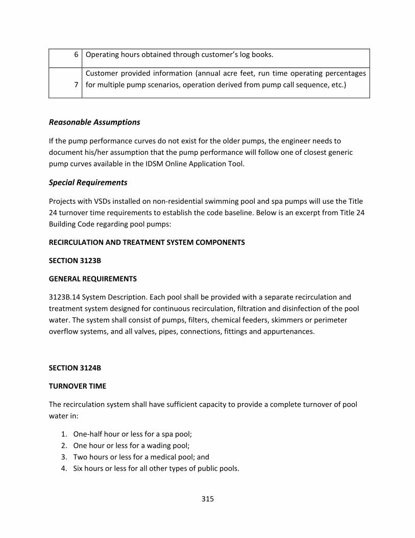
315

6 Operating hours obtained through customer’s log books.

7 Customer provided information (annual acre feet, run time operating percentages for multiple pump scenarios, operation derived from pump call sequence, etc.)


If the pump performance curves do not exist for the older pumps, the engineer needs to document his/her assumption that the pump performance will follow one of closest generic pump curves available in the IDSM Online Application Tool.


Projects with VSDs installed on non-residential swimming pool and spa pumps will use the Title 24 turnover time requirements to establish the code baseline. Below is an excerpt from Title 24 Building Code regarding pool pumps:

RECIRCULATION AND TREATMENT SYSTEM COMPONENTS

SECTION 3123B

GENERAL REQUIREMENTS

3123B.14 System Description. Each pool shall be provided with a separate recirculation and treatment system designed for continuous recirculation, filtration and disinfection of the pool water. The system shall consist of pumps, filters, chemical feeders, skimmers or perimeter overflow systems, and all valves, pipes, connections, fittings and appurtenances.

SECTION 3124B

TURNOVER TIME

The recirculation system shall have sufficient capacity to provide a complete turnover of pool water in:

1. One-half hour or less for a spa pool; 2. One hour or less for a wading pool; 3. Two hours or less for a medical pool; and 4. Six hours or less for all other types of public pools.

316


It is recommended to use IOU preferred tools (i.e. IDSM Online Application Tool (SCE), PSAT, etc.) for energy savings calculations. The pump curve as well as the following input parameters required for these calculations: site information, system design flow, TDH at design flow, and static head.

The following equation can be used to calculate the electric demand for a positive displacement pump:

=

where:

QD = Pump design flow (gpm)

PD = Pump discharge pressure (psig)

ηp = Pump design efficiency

ηe = Drive motor efficiency

And the electric demand of a dynamic pump such as a centrifugal or axial flow pump can be calculated using the following expression.

= (Equation 2)

where:

S = specific gravity of pumped fluid relative to water at 60F

Q = fluid flow (gpm)

H = Total developed head (Ft)

ηp = Pump efficiency


The specific gravity term in this expression, S, is considered constant and is based on the type and temperature of the pumped fluid. With the exception of pump flow, Q, the remaining terms will vary based on pump flow and this expression must therefore be evaluated for each

PUMPkWeP

DD PQηη **1714

**7457.0

PUMPkWeP

HQSηη **3960

***7457.0

317

individual operating mode. It should be noted that the dynamic pump head and efficiency vary depending on pump flow and must be evaluated at each operating point.

Annual energy savings is calculated by subtracting the proposed energy usage from the baseline usage. Incentive values are then calculated as the product of the incentive rate and the estimated energy savings value.

Annual Savings (kWh) = Baseline kWh – Proposed kWh

Incentive Amount ($) = Annual Savings (kWh) * Incentive Rate ($/kWh)

Please refer to Appendix A for details of engineering calculation.

318

PUMPING – SMART WELLS

EEM Description: The installation of new or replacement of existing oil wells with ‘smart’ wells. Smart wells use a slotted casing that skims fluid from relatively oil-rich zones, increasing the ratio of oil:water that is pumped to the surface. The fluid extracted from the well passes through an oil/water separator where the water is moved to the product water storage tank by a second pump (surface pump). This stored water is then re-injected underground by a third pump (product water injection pump). The selectively slotted casing decreases energy demand by reducing the amount of water that is pumped by all three of the pumps since less water is removed from the well per unit of oil product. Work or Product: BBLS of oil Load Influences: Depends on pump production rate, oil field reservoir, geological conditions, and groundwater elevation. Performance Influences: The improvement in performance over standard well completion is largely dependent on the oil:water ratio.

<= Im

pact

kW

h/yr

Constant Load?

Yes No


Yes No Yes No

0 to

250

,000

Not Typical


Calculations

Geologist’s Technical Modeling

Measurements

Oil and water production rates

Not Typical


Calculations


Measurements


250,

000

to 1

,000

,000

Not Typical


Calculations


Measurements


Not Typical


Calculations


Measurements


319

> 1,

000,

0000

Not Typical


Calculations


Measurements


Not Typical


Calculations


Measurements



Obtain all the required inputs for the energy calculation including number of wells, well identification number, motor horsepower (hp), fluid depth, average daily production (barrels of oil per day, bbls/day), annual operating hours, oil:water ratio, and specific gravity of well product.


Daily oil/water production rates should be provided both pre and post-installation for a minimum period of one month. For new installation measures, production rates will be initially estimated and then confirmed post-installation.


Savings should be calculated based on the lower annual oil production of either the standard well or the smart well.


In the case where a well is being converted to a smart well from a standard (or existing) well, the measure is considered a Retrofit Add-on (REA) and as such, a single baseline for the control system should be used. The actual field baseline operating conditions are used to calculate the baseline kWh (motor horsepower, pump efficiency, annual operating hours, and oil to water ratio). In the case where a well is being installed for the first time as a smart well, the expected operating conditions of a standard well serve as the baseline. The expected flow rate and oil:water ratio of a standard well can be estimated based on a geologist’s technical modeling report or other engineering forecast methods.

Estimated production data can be obtained, in some cases, from the California Department of Conservation, Division of Oil, Gas, and Geothermal Resources website:

320

http://opi.consrv.ca.gov/opi

Operating Hours System operating hours for the pre-installation estimate may be based on existing operation if a standard well is being converted to a smart well. For new wells being installed as smart wells, operating hours are predicted by a geologist’s technical model or based on estimated operating schedules. The reported annual runtime should take into account any expected variations in schedule or production, including routine repair or maintenance.


When engineering calculations are performed all assumptions made by the engineer and equations used in the calculations must be well documented and supported. For example, the assumed number of wells, baseline motor load factor and efficiency, pump specifications, oil:water ratio, and annual runtime need to be reasonable and substantiated.

Although metering is not required, savings calculations are likely to be more accurate if meters are installed to measure true kW consumed at the three pump motors. If metering is not able to be conducted, it is recommended that hydraulic head be calculated based on total dynamic head rather than the vertical depth of the well.


The total energy consumed in the process of product oil extraction, separated water treatment, and re-injection includes three pumping systems: the lift pump, the surface pump, and the product water injection pump. The energy use for each pump is calculated for both standard (existing) and smart well configurations, as exemplified by the following equations:

𝐴𝑛𝑛𝑢𝑎𝑙 𝐸𝑛𝑒𝑟𝑔𝑦 𝑈𝑠𝑒 = 𝑃𝑙𝑖𝑓𝑡 + 𝑃𝑆𝑢𝑟𝑓𝑎𝑐𝑒 + 𝑃𝑅𝑒−𝑖𝑛𝑗𝑒𝑐𝑡

with,

𝑃 = 𝑘𝑊𝑃𝑈𝑀𝑃𝑥 𝑡

where:

t = annual runtime of the pump in (hrs/yr)

The electric demand of a dynamic pump, such as a centrifugal or axial flow pump, can be calculated using the following expression:

http://opi.consrv.ca.gov/opi�

321

=

where:

S = specific gravity of pumped fluid (dependent on oil:water ratio)

Q = fluid flow (gpm)

H = Total developed head (Ft)

ηp = Pump efficiency


The estimated energy savings is based on the lower amount of the annual oil production of either the smart well or the standard well, shown by the following equation:

𝑘𝑊ℎ 𝑠𝑎𝑣𝑖𝑛𝑔𝑠 = |𝑙𝑜𝑤𝑒𝑟 𝑜𝑓 𝑃𝑅𝑆𝑇𝐷 𝑜𝑟 𝑃𝑅𝑆𝑀𝑇|𝑥 �𝐸𝑆𝑇𝐷𝑃𝑅𝑆𝑇𝐷

− 𝐸𝑆𝑀𝑇𝑃𝑅𝑆𝑀𝑇

�

where:

PR = total yearly oil production (gal/yr)

STD = Standard well

SMT = Smart well

Assuming the fluid (oil and water) does not have a high total suspended solids (TSS) content, neither the flow rate nor the current draw are expected to change due to deposition on the piping system. However, time of year may affect groundwater elevation, so the oil bearing zone might not always be consistent with the newly selected slotted casing. Therefore the quantity of fluid that drains into the casing might not be the same every day. As such, calculations should account for expected or observed changes in flow or oil/water production.

PUMPkWeP

HQSηη **3960

***7457.0

322

PUMPING – CONTROLS MILKING VACUUM PUMP –VSD (PM-14041)

EEM Description: Replacement of existing milking vacuum pump system with VSD controlled milking system Work or Product: Brake Horsepower, Vacuum Load Influences: Mass flow requirements, milk flow Performance Influences: Variable load

<= Im

pact

kW

h/yr

Constant Load?

Yes No


Yes No Yes No

0 to

250

,000



-Variable Speed Drives for Dairy Vacuum Pump

Measurements

None

250,

000

to 1

,000

,000



-Variable Speed Drives for Dairy Vacuum Pump

Measurements

None

> 1,

000,

.000

0

Not Typical Not Typical Not Typical Not Typical


Obtain manufacturer’s specification sheet and other data for the proposed system, including site data, dairy milk production, and milking hours. Obtain existing vacuum system data, including motor nameplate data. Verify if there are existing auxiliary motors and if they will remain in service or if they will be removed or upgraded.

Please refer to section 2.2.25 in the 2013-14 Statewide Customized Offering Procedures Manual for details

323


Measurements are not typically required for dairy vacuum pump systems.


Typically, dairy farm applications do not include production changes. In case there are production changes, they should be documented and verified. If using the IDSM Online Application Tool, the production change should be indicated in terms of operating hours per day (milking hours per day).



The baseline using only the existing vacuum system parameters is determined using the following: motor hp, motor efficiency, vacuum pump type and operational hours. If there are additional motors in the site that also comprise part of the system such as milk pumps, they are also considered in the baseline. The additional motors may or may not be part of the upgrade, and that is also taken into account when estimating the energy savings. The vacuum pump type may also be changed from the existing type.

The vacuum pump type should be specified as turbine, water ring, blower or vane. The motor efficiency should be specified in terms of NEMA efficiency (minimum EPACT efficiency) or ‘Premium Efficiency’ and horsepower.

Operating Hours

The milking hours per day are considered the operating hours. For dairy farms, they usually consist of up to three four hour shifts. The hours are usually verified from site personnel.


In a dairy farm, the milking schedule is usually fixed in a long-term pattern, since dairy herd sizes are stable. Therefore, operational hours should remain the same before and after

324

measure installation. Typically, the new motors will be rated a lower hp than the existing motor.


There are no special requirements other than to verify existing equipment and operational hours.


The energy savings are calculated using existing motor horsepower and efficiency; 90% motor loading (based on survey data for dairy vacuum pump systems) and operational hours; proposed motor horsepower, efficiency and operational hours. Additionally, vacuum pump types are also evaluated based on their efficiency. If the vacuum pump type remains the same, e.g. water ring existing/ water ring proposed, then, there is no adjustment. However, if the vacuum pump type changes, the efficiency values will be used to account for performance differences. Based on dairy farm surveys, relative efficiency factors were determined for the four vacuum pump types:

Pump Type Efficiency Factor

Turbine 1.00000

Water Ring 0.50979

Blower 0.45070

Vane 0.4324

The additional motors will also be taken into account for the energy savings estimate

The procedure for determining the baseline energy is:

1-determine demand (using existing system parameters)

Demand (kW) = motor hp * 0.7456 kW/hp * 0.9 / motor efficiency

2- determine baseline energy usage

kWh/yr = Demand (kW) * operational hours/yr

3- determine additional usage by additional motors:

kWh/yr (additional) = motor hp /motor efficiency* 0.7456kW/hp * operational hours/yr

325

The total of steps 2 and 3 (if needed) is the baseline energy use.

The proposed energy use is computed as follows:

1- determine demand (using proposed system parameters)

Demand1 (kW) = motor hp/motor efficiency * 0.7456 kW/hp * 0.9

Note if the new hp rating is less than the existing, do not multiply by 0.9

1.1 – modify demand by the vacuum pump efficiency factor ratio, proposed eff/existing eff (from table above)

Demand2 (kW) = Demand1 (kW) * (Prop Eff Factor)/(Existing Eff Factor)

Note this takes into account changes in vacuum pump efficiency.

1.2- modify demand to account for VSD. Based on dairy farm tests, the typical VSD savings is 46.9 %

Demand 3 (kW) Demand 2 * 0.469

1.3- modify demand if the additional motors in baseline case will remain

Demand4 (kW) = motor hp/motor efficiency * 0.7456 kW/hp * 0.9

Do this for each additional motor if more than 1

2 Determine proposed energy use:

kWh/yr (proposed) = (Demand3(kW) + Demand 4(kW) ) * operational hours/yr

The estimated energy savings are:

kWh/yr (baseline) – kWh/yr (proposed) = kWh/yr (savings).

326

PUMPING – CONTROLS POCs FOR OIL WELLS (PM-70932)

EEM Description: This EEM includes savings for the installation of pump-off controllers (POCs) on sucker rod pumping (SRP) systems. Pump-off controllers save energy by reducing the amount of time that the oil well pumping unit operates to match the flow conditions of well. Typically, these wells operate around the clock regardless of their production level. The pump-off controller operate the pump until reduced volumetric efficiency is sensed due to reduced flow of oil in the well, at which the pump is again operated. The pump-off controller uses a smart logic control unit which analyzes accumulated run and off times of the pump to determine the optimum off time for the best well production. The off-time is continuously adjusted based on the inputs from the latest operation information. This EEM is approved only for installations by minor oil producers. Consult Engineering Analysis & Support (EAS) to determine if an oil producer is considered a minor oil producer. Work or Product: BBLS of oil (usually a petroleum water mix) Load Influences: Depends on production rate, Field oil reservoir and geological conditions, well volumetric efficiency and flow. Performance Influences: Smart logic control type, pumped oil viscosity, stroke rate, Field oil reservoir and geological conditions

<= Im

pact

kW

h/yr

Constant Load?

Yes No


Yes No Yes No

0 to

250

,000


Acceptable Methods IDSM Online Application Tool Industrial Pump System

Controls -

WPSCNRMI0006 Measurements

None

250,

000

to 1

,000

,000



Controls -


Two Weeks oil barrel production rate

(Duration Depending on Variability in Performance &

Load)

327

> 1,

000,

.000

0



Controls -


One Month of oil barrel production rate (Duration

Depending on Variability in Performance & Load)


• Obtain all the required inputs of the IDSM Online Application Tool including number of wells, well identification number, motor horsepower (hp), average daily production (barrels of oil per day, bbls/day), annual hours, pump diameter (inches), stroke length (inches) and strokes per minute (spm).


Please refer to section 2.2.20 in the 2013 Statewide Customized Offering Procedures Manual for details.


Measurements will be required for estimated annual kWh savings of more than 250,000 to establish the post-installation operation and to verify savings after the measure is completed. The measured data will be for a period of two weeks (250k <annual kWh<1000k) to one month (annual kWh>1000k) at intervals not greater than 15 minutes (averaged) for total number of wells including:

• Pump power consumption (kW) and sucker rod speed (spm)

• Average daily production (barrels of fluid per day, bbls/day)


When monitored data shows baseline to post-installation production changes, the energy savings should be calculated based on the monitored post-installation production.


328

This measure is typically considered a Retrofit Add-on (REA) and as such a single baseline for the control system should be used. The actual field baseline operating conditions is used to calculate the baseline kWh (motor horsepower, load factor, motor efficiency and annual operating hours). The baseline condition for a sucker rod pump is continuous operation of the pump regardless of its volumetric efficiency.

Effective May 1, 2013, the following are new requirements for electric submersible pumps and pump control technologies in the oil industry.

Energy Division (ED) conducted an industry standard practice (ISP) study that established new pump control baselines for three (3) oil pump types: rod beam pumping, electric submersible pumps (ESP), and progressing cavity pumps (PCP). SCE also conducted a similar ISP study, which evaluated two measures: 1) replacing standard electric submersible pumps (ESP) with high efficiency ESPs, and 2) adding VFDs to ESPs in new wells and in existing wells. The tables below summarize the results from both studies.

Table 17. Summary of ISP Findings for Artificial Lift Pump Control Technologies

Pump Type (Install Type) Baseline Method of Control

Major Oil Producers Minor Oil Producers

Rod Beam Pumping (New) POC Continuous Operation

ESPs (New) VSD VSD

ESPs (Existing)* Throttling Throttling

PCPs (New) VSD VSD

* See SCE ISP Study for allowable applications for this baseline.

Table 18. ISP per Installation Type for High Efficiency ESPs

Install Type ESP Retrofit Baseline

ROB/NEW High Efficiency ESP

Major and minor oil producers are defined by their respective fraction of overall California oil production. The 2.5% oil production threshold is based on 2012 DOGGR data and may be updated by ED in a future study.

• A major oil producer generates more than 2.5% of the California oil production in 2012.

• A minor oil producer generates less than 2.5% of the California oil production in 2012.

Oil producers that generate less than 2.5% of the California oil production, but are affiliates of major oil producers must be considered major oil producers. ED believes that resources

329

available from financial and/or management control of firms influence operating and capital investment practices.

An affiliate is a firm that is related to another firm by any of the following circumstances:

a. Common shareholdings or other means of control b. Shared office or warehouse facilities, equipment, systems, and/or employees c. Shared or common owners, officers, and/or directors d. A financial relationship, including loans and assistance to meet bond, security or credit

requirements e. A contractual relationship, including assignment or transfer of rights, responsibility or

property f. Family ties (spouse, parent, child, or sibling) g. An arrangement with any other business to assign a contract, in whole or in part.

(Excluding those with a public financial institution.) h. An agent/broker relationship under which the firm is authorized to transact business

for, or manage/control the affairs of another firm or individual, or act for them under the contractual relationship of agency.

If a major oil producer terminates a relationship with an affiliate that produces less than the threshold, the affiliate is still considered a major oil producer. Operating Hours

System operating hours for the pre-installation estimate may be based on operation recorded during the baseline period. For final savings estimates, operating hours should be based on the operating hours recorded during the post-installation monitoring period, and should also take into account any expected variations in schedule or production over the first year of post-installation operation.

A 98% adjustment factor must be applied to the operating hours of pumps in oil fields for measures claiming 8,760 operation. This factor reduces the operating hours from 8,760 to 8,585 hours per year. This adjustment factor is based on the reference study, "Evaluation of the Energy Efficiency Services Electricity Consumption and Demand Reduction in Oil Production Program" by Quantec, prepared for GEP.21

21 Lee, Allen, Ken Seiden, and Elaine Prause. Evaluation of the Energy Efficiency Services for Electricity Consumption and Demand Reduction in Oil Production Program. Tech. N.p.: Quantec, LLC, 2004.

Pumps used in industries outside of the oil industry are not subject to the 98% adjustment factor.

330


When engineering calculations are performed all assumptions made by the engineer and equations used in the calculations must be well documented and supported. For example, the assumed number of wells, baseline motor load factor and efficiency, pump specifications, stroke speed, gross production and annual runtime need to be reasonable and substantiated by facilities personnel.

Production data can be obtained in some cases from the California Department of Conservation, Division of Oil, Gas, and Geothermal Resources website:

http://opi.consrv.ca.gov/opi


In the case of horizontal wells, the VSDs are used instead of POCs and offer similar benefits without having to turn off the pumping unit.


The estimated savings is based on a simplified empirical model, which correlates volumetric efficiency, percentage runtime and percentage energy use.

The first step is to determine the current volumetric efficiency. The volumetric efficiency is the ratio of the actual production to the theoretical production.

EQ-1

where,

VE = volumetric efficiency of well, after stroke speed and length modifications

PRa = average daily oil production, based on last 12 months of production data

PRt = theoretical daily oil production, based on Equation-2

The gross production should be based on the last 12 months of production. The theoretical production is calculated using the following equation.

EQ-2

a

t

PRVE =PR

2

t

(D /12)3.14 (SL /12) SPM 7.48 60 242PR =

42

× × × × × ×

331

where,

D = pump diameter (inches)

SL = stroke length (inches)

SPM = strokes per minute

Once the volumetric efficiency has been calculated, the percentage energy use can be estimated using the following empirical equations.

EQ-3

where,

RT% = percentage runtime

The equation used to estimate the percentage energy use after a well has been retrofit with a pump-off controller is

EQ-4

where,

E% = percentage energy consumption after installation

The last step is to estimate the baseline energy consumption. Based on several studies, the average loading of 194 motors was 20%.

EQ-5

Where,

P = average power demand of the motor (kW)

HP = motor horsepower (user input)

LF = load factor (assumed to be 0.20)

Eff = the motor efficiency (assumed to be 0.75)

The baseline energy consumption is

%RT = 8.336 0.956 VE+ ×

% %E = 20.76 0.907 RT+ ×

0.746 HP LFP =Eff× ×

332

EQ-6

Where,

Hrpre = average baseline operating hours per day

Epre = baseline energy consumption (kWh)

The post-installation energy consumption is

EQ-7

Where,

Epost = post-installation energy consumption (kWh)

Finally, the energy savings is

EQ-8

Where,

Esaved = energy savings (kWh)

The demand savings are based on the study that compared energy savings to coincidental peak demand reduction. The empirical relationship recommended by the study is

EQ-8

Where,

DF = POC Demand Factor

This equation estimates the percent demand of the well with the POC. Therefore, the post installation peak demand is

And the peak demand savings are

pre preE = P Hr×

post % preE = E E×

saved post preE = E - E

post

pre

EDF = 8.4% +

E

post prekW = DF kW×

saved pre postkW = kW kW−

333

PROCESS – EFFICIENT BATTERY CHARGER (PR-69844)

EEM Description: The installation of efficient battery chargers for commercial applications and large non-residential applications (input over 2 kW). Work or Product: Reduced total energy use for charging equipment. Load Influences: Battery type and capacity, attached equipment quantity, power conversion factor. Performance Influences: Charger load capacity, Charge return factor, power conversion factor, power factor, system load, equipment charge capacity, battery charge control design efficiency.

<= Im

pact

kW

h/yr

Constant Load?

Yes No


Yes No Yes No

0 to

250

,000


Calculations or Monitor Data

Measurements

AC charger input watt-hours, DC charger output watt-

hours, ampere-hours into & out of battery, power factor.

Not Typical


Calculations or Monitor Data

Measurements



Not Typical

250,

000

to 1

,000

,000



Measurements



Not Typical



Measurements



Not Typical

> 1,

000,

.000

0

Not Typical

Not Typical

Not Typical

Not Typical


For efficient battery chargers, obtain the nameplate ampere-hours into and out of the battery charger. The charge return factor is then defined as the ratio of ampere-hours into the battery over the ampere-hours out of the battery. Obtain the power conversion efficiency of the

334

electronics used to charge the battery, defined as the power out of the charger over the power into the charger.


The CEC battery charger system test procedure enables testing of all types of battery charger systems regardless of end use and has two parts. Part 1 applies primarily to small residential and commercial battery charger systems and Part 2 applies to larger industrial battery charger systems. Three modes of charge should be tested in both parts – energy consumption in charge mode, maintenance mode, and no battery mode.

Part 1 specifies the battery charger undergoes a 24-hour charge cycle and a 5-hour discharge cycle. The energy delivered from the battery during discharge can be compared to the energy consumed by the charger during charge, the result of which can be defined as the battery charger efficiency. Maintenance mode consumption should be measured by integrating the energy usage over the last 4 hours of the testing period, while no battery mode consumption is similarly measured for 10 minutes.

Part 2 specifies the large battery charger undergoes three discharge/charge cycles using three different depths of discharge, 100%, 80%, and 40%. The measurements distinguish between energy lost in the charger and energy lost in the battery. The charge return factor is used to quantify battery charger performance as defined above and represents how well the battery charger charges the battery. The power conversion efficiency and power factor should be recorded for three points during recharge, maximum, median, and minimum power levels. The energy consumption should also be measured for 72 hours of maintenance mode and one hour of no battery mode.


Changes from baseline to post-installation production would occur if the facility has more or less batteries in ports being charged at a given time. The inventory of batteries and battery chargers should be counted in the post-installation inspections as the production loads will be based on the post-installation number of batteries to be charged.


For a project to be eligible for the Statewide Customized Offering, any existing equipment required to establish the project baseline must be operating and available for inspection.

For commercial battery charging systems, the battery capacity and number of charger ports, average maintenance power, and no battery power should be determined for the baseline consideration.

335

For large non-residential battery charging systems, the number and type of batteries, battery capacity, battery depth of discharge, and equipment operational hours need to be determined to establish the baseline. Additionally, the type of battery charger technology, charge return factor, and power conversion efficiency need to be established.

Table 19 highlights the Title 20 effective dates for various battery charger applications. Calculations for non-residential projects should not use the residential code baseline. The current non-residential baseline is the industry standard practice. Effective 1/1/2014, Title 20 will be in effect for the large non-residential battery charger system.

Table 19. Title 20 - Energy Efficiency Standards for Battery Charger Systems

Table 20 and Table 21 below provide the applicable Title 20 Codes for small and large battery systems respectively.

336

Table 20 Small Battery Charger Systems

Table 21 Large Battery Charger Systems

337

Operating Hours

System operating hours for the pre-installation estimate may be based on operation recorded during the baseline period. For final savings estimates, operating hours should be based on the operating hours recorded during the post-installation monitoring period.

For large battery charger systems the typical charge times range from 8 to 10 hours* per battery and spend the majority of their time in charge mode, actively charging the battery. The number of times the battery charger is used per week needs to be determined in addition to the battery specific charge time.

*2010-2011 CASE Initiative for Analysis of Standards Options for Battery Charger Systems, Submitted to PG&E, SCE, SDG&E October 1, 2010.


If the annual energy savings are less than 250,000 kWh per year, it is reasonable to use estimated equipment operating hours and battery charger specifications (charge return factor, power conversion efficiency, etc) in lieu of monitored data. If the annual energy savings are greater than 250,000 kWh per year, it is reasonable to assume that a one week monitoring period, to establish the duty cycle in addition to how many batteries are being charged per day, will provide a high degree of confidence in the data collected.


The new standards apply to all battery chargers except those:

1. Used to charge electric vehicles, not including golf carts, or low speed vehicles as defined in the Division 1 of the California Vehicle Code

2. Designated as medical devices

3. Used to charge illuminated exit signs

4. Designed for a stationary power application

5. Utilized as battery analyzers

6. That are voltage/frequency independent (i.e. uninterruptible power supplies).

Power measurements must be performed using a three-phase power meter, capable of recording volts, amps, power factor and kW. Output must also be recorded to establish the actual specific energy usage.

338


Energy savings calculations for a battery charger are dependent on the charge return factor ratio, the power conversion efficiency of the electronics, and the battery depth of discharge and power factor. Prior to implementation, detailed engineering calculations and clearly supported assumptions must be submitted with the application. The charge return factor is determined from the ratio of ampere-hours into the battery over ampere-hours out of the battery. The power conversion factor is the power out of the battery charger over the power into the battery charger.

339

PROCESS – FANS

EEM Description: This includes direct replacement of a fan with a high efficiency fan or including a more efficient belt drive and/or blades. Energy Savings are realized by eliminating losses due to mechanically throttling air flow, better operation near or at best efficiency point and/or installing a more aerodynamically appropriate fan. Work or Product: Air flow or air horsepower Load Influences: Depends on flow controls, changes in gas characteristics and/or process demands. Performance Influences: Primarily load, but performance also can be influenced by flow controls and/or changes in gas characteristics.

<= Im

pact

kW

h/yr

Constant Load?

Yes No


Yes No Yes No

0 to

250

,000


Tool and Fan System Assessment Tool (FSAT)


Measurements None


Acceptable Methods IDSM Online Application Tool and Fan System Assessment Tool (FSAT) and Engineering

Spreadsheet Calculations

Measurements None

250,

000

to 1

,000

,000




Measurements

Two Weeks of Power Consumption or CFM



Acceptable Methods IDSM Online Application Tool and Fan System Assessment Tool (FSAT) and Engineering

Spreadsheet Calculations

Measurements Two Weeks of Power Consumption or CFM


Load)

> 1,

000,

.000

0



Measurements

One Month of Power Consumption or CFM



Acceptable Methods IDSM Online Application Tool and Fan System Assessment

Tool (FSAT)

Measurements One Month of Power Consumption or CFM


Load)

340


• Obtain characteristic performance curve from the manufacturer tech sheet for the existing fans.

• Obtain all the input data that are required for IDSM Online Application Tool /FSAT simulation tool including, but not limited to fan total static pressure, drive motor efficiency and fan efficiency at the fan’s design point.


Please refer to section 2.2.29 in the 2013-14 Statewide Customized Offering Procedures Manual for details.


Measurements will be required for estimated annual kWh savings of more than 250,000 to establish the post-installation operation and to verify savings after the measure is completed. The measured data will be recorded for a period of two weeks (250k <annual kWh<1000k) to one month (annual kWh>1000k) for the total fan system, including fan motor power consumption (kW), flow (CFM) and static pressure. The suggested sampling rate for these parameters is 1 minute, with average values recorded at intervals not greater than 15 minutes.





341

Operating Hours

Fans operating hours must be based on the baseline and post-installation conditions.


If the fan performance curves do not exist for the older fans, the engineer needs to document his/her assumption that the fan performance will follow one of closest generic fan curves available in the IDSM Online Application Tool.


None


It is recommended to use IOU preferred tools (i.e. IDSM Online Application Tool (SCE), FSAT, etc.) for energy savings calculations. The fan performance curve as well as the following input parameters required for these calculations: site information, inlet and ambient air temperatures, fan system type, number of fans, system design (maximum) flow, system total static pressure at maximum flow and static efficiency.

The electric demand of a fan is calculated using the following expression.

FANkW =

Where:

QF = Fan flow (CFM)

Ps = Fan static discharge pressure (inches Wg)

Kp = Compressibility Factor (initially set to 1.0)

ρin = Air density corrected for fan inlet conditions

ρstd = Air density at standard conditions (0.075 lbs/ft3)

ηF = Fan efficiency @ operating conditions

ηe = Electric drive motor efficiency

ηd = Drive efficiency (if applicable)

stdedF

inSFp

PQKρηηη

ρ****6.6349

****7457.0

342

Fans exhibit dynamic performance characteristics such that fan total static pressure (PS), brake horsepower and static efficiency (ηF) vary with flow. These performance parameters must therefore be calculated for each operating point (for use in above equation). Fan total static pressure and efficiency are typically characterized in a fan performance curve. These curves are generated by the fan manufacturer using test data and are used to determine the fan operating point (pressure and efficiency) under varying flows and speeds.

The savings associated with replacement of an existing fan with a fan of the same or different type, having a higher efficiency is calculated for each operating point in the same manner as described above for baseline energy use. The difference being that the new fan information (fan type, fan efficiency, etc.) is substituted for the existing fan information.

If both the fan and motor are being replaced the savings associated with replacement of the existing fan drive motor with a motor having a higher efficiency is calculated in the same manner as described above baseline energy use. The exception being that the new motor efficiency is substituted for the existing motor efficiency.

The electric demand of a fan operating with an improved belt drive is calculated using the same expression above with the exception that the new drive efficiency value is used in the drive efficiency term (ηd) in the above equation.

Annual energy savings is then calculated by subtracting the proposed energy usage from the baseline usage. Incentive values are then calculated as the product of the incentive rate and the estimated energy savings value.

Annual Savings (kWh) = Baseline kWh – Proposed kWh

Incentive Amount ($) = Annual Savings (kWh) * Incentive Rate ($/kWh)

Please refer to section 2.2.29 in the 2013-14 Statewide Customized Offering Procedures Manual for details of engineering calculation.

343

PROCESS – COMPRESSED AIR

EEM Description: This EEM includes air compressor retrofit, air compressor consolidation, increased storage for air compressors, right-sizing air compressors, other compressed air applications to improve compressor efficiency and reducing unnecessary compressor operation. Work or Product: Volumetric Flow – standard cubic feet per minute (scfm) - of compressed air. Load Influences: Production demand, unregulated demand, leaks, open blowing and other inappropriate uses. Performance Influences: Ambient conditions, system pressure, control strategy, load variations.

<= Im

pact

kW

h/yr

Constant Load?

Yes No


Yes No Yes No

0 to

250

,000


Acceptable Methods AirMaster+

IDSM Online Application Tool Custom Engineering


Short term (seven days minimum)

Electric demand (kW) or Production rate (acfm)

250,

000

to 1

,000

,000





Short term (seven days minimum, sufficient to capture any production

variation or cycle) Production rate (acfm) Electric demand (kW)

Compressed Air Supply System Efficiency (CASE)

344

> 1,

000,

.000

0


Not Typical




Medium term (one month minimum, sufficient to capture any production

variation cycle) Production rate (acfm) Electric demand (kW)

Compressed Air Supply System Efficiency (CASE)


Obtain manufacturer’s specifications (CAGI “Compressed Air & Gas Institute” datasheets), if available, for both existing and retrofit equipment.

If CAGI datasheets are not available, specifications should include:

• Manufacturer

• Compressor type

• Control type (load/unload, inlet modulation, vfd, etc.)

• Drive motor nameplate rating (hp)

• Full load operating pressure (psig)

• Rated capacity at full load operating pressure (acfm)

• Total package power at rated capacity and full load operating pressure (kW)

• Total package power at zero flow (unloaded kW)

• Specific package power at rated capacity and full load operating pressure (kW/100 acfm)

• Location of system (city). The IDSM Online Application Tool uses this to determine the average inlet pressure and temperature for the compressed air system.

For an old air compressor, the total package power at zero flow for the baseline unit may not available. If this is the case, the unloaded kW can usually be found/captured using monitored data if the air compressor unloads during the monitored period. However, if the compressor

345

never unloads during the monitored period, the default value available in AirMaster+ for an air compressor similar to the baseline air compressor should be used. When applicable, attain process flow diagrams of the affected system.

It is not recommended or preferred to use CAGI data for a representative sample manufacturer for like type equipment (i.e. different from existing or proposed) due to the fact that the performance characteristics of like equipment can vary greatly. Two compressors of equal rated capacity and similar control type may have different specific package power (efficiency) and operating pressures. When modeling a compressor retrofit, if specifications are not available for the baseline compressor, the AirMaster+ default configuration for a compressor of similar size, control type and discharge pressure can be used because the AirMaster+ default is the minimum standard efficiency for savings calculations. For the proposed equipment, it is much more important to use inputs that are as accurate as possible and manufacturer’s specifications should be available for any new compressor.


For savings estimates, both AirMaster+ and the IDSM Online Application Tool require an hourly load profile for each compressor, in either kW or acfm. Both models allow for multiple day types and seasonal operation. The user must identify weekday and weekend profiles. Model results may be confirmed by spot measurements or short term monitoring for lower complexity projects. Higher complexity projects may require longer term monitoring of both production and electric demand to verify system efficiency improvements.

Other data requirements:

• Nominal system operating pressure

• Receiver and total system storage volume

• Elevation, average inlet pressure (psia) and temperature (deg F), for AirMaster+

The IOUs developed an Industrial Compressed Air Supply System Efficiency (CASE) index as a stand-alone value for compressor central plant efficiency, which can be used to verify the actual energy savings for a compressed air project. CASE is not a modeling or simulation tool, but a method for quantitatively evaluating the energy savings using measurements obtained from the pre- and post-installation systems. The index captures the overall efficiency of a compressed air system’s supply side under typical plant operating conditions. Essentially, the index is a ratio of standard cubic feet (scf) of compressed air supplied by the central plant to the total number of kWh supplied over a given cycle period. To evaluate the CASE index the system flow should, ideally, be measured with a thermal mass flow meter at a point downstream of the

346

supply side storage and any pressure/flow control devices. This value, along with the electric demand of each compressor, should be measured at 15 second intervals recording one minute averages. The CASE index is then evaluated as the system efficiency in units of scf/kWh.


Compressed air demand (production) may change from the baseline period to post-installation (verification) period for several different reasons. Depending on these reasons the changes must be addressed accordingly in the savings calculations.

If compressed air demand decreases because of decreased production of the facility’s end product, then the effect of this decrease must be subtracted from the baseline energy use. If compressed air demand decreases due to leak repairs, there will be a program specific allowance that must be considered when determining the baseline energy use.

If compressed air demand decreases due to other demand side improvements that save energy, such as replacing pneumatic pumps or motors with equivalent electric equipment or reducing the system pressure to lessen the effects of unregulated users, then the net effects of these improvements may be included in the final savings.



One must first determine if the measure is eligible for early retirement (RET). If the measure does not qualify for early retirement (RET), then a single baseline is determined and must use the forecasted equipment load and an appropriate minimum efficiency standard to establish baseline performance. An acceptable minimum efficiency standard must be a government minimum efficiency standard or, if a minimum standard efficiency is not available, the current industry practice. If early retirement does apply, then two separate baselines must be determined. The first baseline shall be determined using the pre-existing equipment efficiencies. The second baseline shall be determined using forecasted equipment load and an appropriate minimum efficiency..

For new installations or new loads using high efficiency compressors, the baseline equipment efficiency will be the AirMaster+ efficiency described above.

For compressor of a size or type, such as large (>400 HP) multistage reciprocating compressors used in PET bottle manufacturing, that are not included in the Airmaster+ catalog the baseline efficiency should be the OEM rated efficiency of the existing equipment.

347

Operating Hours

System operating hours for the pre-installation estimate may be based on operation recorded during the baseline period. For final savings estimates, operating hours should be based on the operating hours recorded during the post-installation monitoring period, and should also take into account any expected variations in schedule or production over the first year of post-installation operation.


The replacement of compressed air systems with industrial blowers is eligible as a Customized measure under solution code PR-38532. A measure that is adding a blower without removing an air compressor is eligible if the existing compressed air system is equipped with a VFD and there is an overall reduction in the compressed air consumption.


Analysis using AirMaster+ should only be performed by those familiar with the software application.


The following calculation should be used to determine energy savings of a compressed air measure:

Savings = Baseline Energy – Reporting Period Energy ± Adjustments

Where;

Baseline Energy = Baseline Intensity (kW/scfm) * Baseline Production Rate (scfm) * Annual Operating Hours

Reporting Period Energy = Reporting Period Intensity (kW/scfm) * Reporting Period Production Rate (scfm) * Annual Operating Hours

Adjustments = Baseline efficiency adjustments and any adjustments required to make the baseline period conditions and production equal to the reporting period conditions and production.

And;

ACFM is the volumetric flow rate of air at the system pressure.

SCFM is the volumetric flow rate of air at some standard temperature and pressure

348

ACFM = SCFM [Pstd / (Pact - Psat Φ)](Tact / Tstd)

ACFM = Actual Cubic Feet per Minute

SCFM = Standard Cubic Feet per Minute

Pstd = Standard absolute air pressure (psia)

Pact = Absolute pressure at the actual level (psia)

Psat = Saturation pressure at the actual temperature (psi)

Φ = Actual relative humidity

Tact = Actual ambient air temperature (deg R)

Tstd = Standard temperature (deg R)

AirMaster+ and the IDSM Online Application Tool are not capable of analyzing all possible compressed air system upgrades. For projects that cannot be modeled using these tools, or if the analyst is not familiar with them, Custom Engineering Calculations, in the form of a live spreadsheet, may be acceptable. If Custom Engineering Calculations are used, the Baseline and Reporting Period energy calculations must account for:

• Compressed air demand

• Inlet conditions

• Overall system efficiency

• Changes in system controls and control strategy

• Changes in system pressure

• Baseline to Post-Installation Production Changes, as described above

• Minimum baseline efficiency, as described above in “Baseline Considerations”

349

PROCESS – DRYER

EEM Description: Equipment that produces and applies heated air (convective or direct drying) to reduce air relative humidity. This EEM includes high efficiency air dryer, cycling refrigerated and desiccant dryers Work or Product: Cubic feet per minute of dry air Load Influences: Process demand. Performance Influences: Performance is primarily constant, but occasional parameters such as inlet and outlet humidity and temperatures, air mass flow and controls, may also affect performance.

<= Im

pact

kW

h/yr

Constant Load?

Yes No


Yes No Yes No

0 to

250

,000


Calculations

Measurements None

Not Typical


Calculations

Measurements None

Not Typical

250,

000

to 1

,000

,000


Calculations

Measurements None

Not Typical


Calculations

Measurements None

Not Typical

> 1,

000,

.000

0


Calculations

Measurements Power Consumption &

Production Rates

Not Typical


Calculations

Measurements Power Consumption &

Production Rates

Not Typical

Documentation & Source Information Obtain manufacturer specs sheets of the baseline and proposed equipment involved. The important characteristics are power consumption and processed air flow rate. The equipment is typically rated in CFM capacity of the dryer. Facility production logs or operations information should also be collected to confirm the yearly operation of the facility. When applicable, attain process flow diagrams of the affected system.

350

Measured Data Requirements Measurements are not required since the specs sheets define the operation of the dryer appropriately.

Baseline to Post-Installation Production Changes If the load is expected to change post-installation, the current performance of the existing equipment should be applied to the proposed load in order to determine the baseline consumption. The production is verified through production logs. Unless there is also a compressor replacement air flow monitoring is not performed.

Baseline Considerations One must first determine if the measure is eligible for early retirement (RET). If the measure does not qualify for early retirement (RET), then a single baseline is determined and must use the forecasted equipment load and an appropriate minimum efficiency standard to establish baseline performance. An acceptable minimum efficiency standard must be a government minimum efficiency standard or, if a minimum standard efficiency is not available, the current industry practice. If early retirement does apply, then two separate baselines must be determined. The first baseline shall be determined using the pre-existing equipment efficiencies. The second baseline shall be determined using forecasted equipment load and an appropriate minimum efficiency.

.

Operating Hours System operating hours should, at minimum be calculated based on the existing system and in accordance with the existing operating hours of the facility.

Reasonable Assumptions Dryer replacements are usually bundled in compressed air system upgrades. It is very rare to see the replacement only of a dryer. Often non-cycling refrigerated dryers are replaced with more efficient cycling ones. In such case, the consumption of the non-cycling dryer has to be verified with the manufacturer specifications sheets and often the consumption does not depend on the load. The dryer still consumes the same amount of power when less CFM is required to be dried because the system goes into a hot gas by-pass mode.

Special Requirements None.


351

The following calculation should be used to determine energy savings of a refrigeration upgrade measure:


CFM * kW/100CFM * hrs * 100 = annual kWh

Where;

CFM= average compressed air system cubic feet per minute

kW/100CFM = efficiency of the dryer

hrs = operation hours of the system


352

PROCESS – CHILLER

EEM Description: Process chiller measures include the retrofit or new installation of a high efficiency water-cooled or air-cooled chiller to optimize the system’s operating efficiency. There are four (4) potential replacement scenarios for this measure: water-cooled to air-cooled, air-cooled to water-cooled, water-cooled to water-cooled and air-cooled to air-cooled. Work or Product: Tons cooling Load Influences: Production rate, product characteristics, differential temperature & phase change (if any). Performance Influences: Weather & load.

<= Im

pact

kW

h/yr

Constant Load?

Yes No


Yes No Yes No

0 to

250

,000

Not Typical

Acceptable Methods





Not Typical


Measurements

Short to Extended Duration Power Consumption & Cooling Load (Duration


250,

000

to 1

,000

,000

Not Typical

Acceptable Methods





Not Typical


Measurements

Short to Extended Duration Power Consumption & Cooling Load (Duration


> 1,

000,

.000

0

Not Typical


Measurements



Not Typical


Measurements

Extended Duration Power Consumption & Cooling Load


Load)

353


Obtain performance data from the manufacturer for the proposed chiller. The proposed performance data should be for the expected chiller condenser water entering temperature and chiller evaporator water leaving temperatures. The proposed performance data will be used in the energy savings calculations to estimate the power consumption at each weather bin load. This will be verified with post-installation monitored data. When applicable, attain process flow diagrams of the affected system.


Measurements are required to establish the baseline load and to verify savings after the measure is completed. The measured data will typically be for a period of three (3) weeks at intervals of 15 minutes or less and will include power (kW) and load (CHW flow (gpm), CHW leaving and CHW return temperatures). If the load is constant, only the power (kW) of the system must be monitored. The load of the system must be verified by a spot measurement (CHW flow (gpm), CHW leaving and CHW return temperatures). The measurement period for large impact projects will typically be four (4) to six (6) weeks.


When monitored data shows baseline to post-installation load changes, the energy savings should be calculated based on the monitored post-installation load


Process chillers retrofit measures apply the Title 24 efficiency (or efficiencies from the non-standard centrifugal chiller tables) and standard DOE-2 performance curves to establish baseline energy use. The program does not pay incentives for degraded operation, so measured data cannot be directly used for the standard energy use.

There are four (4) potential replacement scenarios when determining baseline energy performance:

1. Existing water-cooled chiller replaced with an air-cooled unit 2. Existing air-cooled chiller replaced with a water-cooled unit 3. Existing water-cooled chiller replaced with a water-cooled unit 4. Existing air-cooled chiller replaced with an air-cooled unit

Scenario 1 - Water-cooled to Air-cooled Chiller

Although it is rare that a water-cooled chiller is replaced with an air-cooled chiller, the project can be eligible for savings as long as sufficient evidence is provided that the air-cooled unit is in fact more efficient than the existing water-cooled system. The capacity of the current chiller

354

(tons) should be evaluated against current standards to ensure that the code allows for the specified tonnage to be served by an air cooled system. If the code requires the installation of a water-cooled chiller, the project is not eligible. Title 24 currently states that any new unit over 300 tons must be water-cooled; however, units under 300 tons may be air-cooled. If the measure is eligible for RET – Early Retirement and the new unit capacity is less than 300 tons, baseline 1 is the existing water-cooled unit and baseline 2 is the code requirement for a water-cooled chiller with the same capacity as the existing equipment. If the measure is not eligible for RET, it should be evaluated as ROB. In this case the baseline efficiency would be as specified by the current energy code for a water-cooled chiller with the same capacity as the existing equipment. However, if the proposed air-cooled chiller is less efficient than the Title 24 code requirement for a water-cooled chiller, there could be negative savings associated with ROB or RET baseline 2. Additionally, although the ROB baseline and RET baseline 2 are typically a Title 24 code compliant water-cooled chiller, in some cases it can be argued that it is industry standard practice to replace a water-cooled chiller with an air-cooled unit (due to poor water quality or other industry specific reasons). If an air-cooled chiller installation is considered ISP, the ROB baseline and RET baseline 2 may be a Title 24 compliant air-cooled chiller. This may result in a greater savings estimate for RET baseline 2 than RET baseline 1, which is not typical.

Scenario 2 - Air-cooled to Water-cooled Chiller

The capacity (tons) of the existing chiller should be evaluated against current standards to ensure that the code allows for the specified tonnage to be served by an air cooled system. Title 24 currently states that any new unit over 300 tons must be water-cooled; however, units under 300 tons may be air-cooled. If the measure is eligible for RET-Early Retirement, baseline 1 is the existing air-cooled chiller (under and over 300 tons). Baseline 2 is the code requirement for an air-cooled chiller (under 300 tons) or the code requirement for a water-cooled chiller (over 300 tons). Baselines should be considered at the same capacity as the existing equipment. If the measure is not eligible for RET, it should be evaluated as ROB. For ROB, the baseline is the code requirement for an air-cooled chiller (under 300 tons) or the code requirement for a water-cooled chiller (over 300 tons) at the same capacity as the existing equipment.

Scenario 3 - Water-cooled to Water-cooled Chiller

If the measure is eligible for RET – Early Retirement, baseline 1 is the existing water-cooled unit and baseline 2 is the code requirement for a water-cooled chiller with the same capacity as the existing equipment. If the measure is not eligible for RET, it should be evaluated as ROB. In this case the baseline efficiency would be as specified by the current energy code for a water-cooled chiller with the same capacity as the existing equipment.

355

Scenario 4 - Air-cooled to Air-cooled Chiller

The capacity of the current chiller (tons) should be evaluated against current standards to ensure that the code allows for the specified tonnage to be served by an air cooled system. If the code requires the installation of a water-cooled chiller, the project is not eligible. Title 24 currently states that any new unit over 300 tons must be water-cooled; however, units under 300 tons may be air-cooled. If the measure is eligible for RET – Early Retirement, baseline 1 is the existing air-cooled unit and baseline 2 is the code requirement for an air-cooled chiller with the same capacity as the existing equipment. In the case of a unit that is over 300 tons, baseline 1 is the existing air-cooled unit and baseline 2 is the code requirement for a water-cooled chiller with the same capacity as the existing equipment. If the measure is not eligible for RET, it should be evaluated as ROB. In this case the baseline efficiency would be as specified by the current energy code for an air-cooled chiller with the same capacity as the existing equipment.

Operating Hours

The operating hours are based on the monitored data. If operating hours vary depending on season, the customer must submit supporting documentation to verify seasonal operating hours.


When engineering calculations are performed all assumptions made by the engineer and equations used in the calculations must be well documented and supported. For example it should be stated and verified that the monitored period is under typical operation, the weather data used in the calculations represents the location of the facility and a correlation exists between the ambient temperature and load or power (kW) of the process chiller.


Some chillers may be dual use where a portion of the capacity is used for process cooling and a portion of the same chiller is used for space cooling. In a case where the facility’s chiller is used for both process and space cooling loads, the chiller should be held to Title24 efficiencies. When modeling chillers that are dual use, the load amount that will contribute to the process cooling and the amount that will contribute to space cooling will both need to be modeled. The efficiency of the chiller must still comply with the requirements of Section 112, the space conditioning requirements in Section 144, and documentation of the set-up. Any capacity for space conditioning will trigger Title 24 requirements. Chillers used 100% for industrial processes are still subject to Title 24 requirements. The load must still be accounted for and designated as process load. This will adjust the allowable budget (baseline energy will equal

356

the proposed energy) to not have the unit affect the energy compliance margin. All mechanical, lighting, and envelope requirements will still apply in a process load.


Engineering calculations are customized savings estimation methods developed for specific projects. They are permitted for savings estimations, but the assumptions and equations must be well documented and supported. In addition, depending on the measure complexity and impact the calculations should be supported with measured data for baseline and post-installation conditions.

An example of an acceptable engineering calculation method would be a bin analysis. In a bin

analysis, the outdoor temperatures are grouped into bins of equal size, typically 5°F bins and

the number of hours of occurrence is also determined for each bin. The monitored data is used to correlate outdoor air temperature to load. Using the full load nameplate efficiency (or efficiencies from the non-standard centrifugal chiller tables) and standard DOE-2 performance curves the baseline power demand is calculated for each weather bin and multiplied by the corresponding number of hours in the bin to calculate the baseline energy consumption. The proposed energy consumption is calculated in the same methodology, the difference is the power would be calculated using the proposed performance data from the manufacturer.

357

PROCESS – HEAT EXCHANGER

EEM Description: Upgrade of heat exchanger to improve process performance. The upgrade may involve heat recovery with the installation of a new heat exchanger to improve process performance; increasing the surface area of an existing heat exchanger to enhance the heat transfer and improve process performance; or simply remove heat from an electric process to improve process performance. Work or Product: Heat rejection or heat recovery from a process measured in Btu/hr. Load Influences: Variations in the load may result in a variable flow through or variable temperature differential across the heat exchanger. Performance Influences: Heat exchanger losses to the environment would affect the performance of the heat exchanger as a function of ambient temperature .

<= Im

pact

kW

h/yr

Constant Load?

Yes No


Yes No Yes No

0 to

250

,000

Acceptable Methods


Measurements

None

Acceptable Methods

Engineering Spreadsheet Calculations – Use

published fouling factors & bin analysis if rejecting heat

to ambient

Measurements None

Acceptable Methods


Measurements

None

Acceptable Methods

Engineering Spreadsheet Calculations – Use published fouling factors & bin analysis if rejecting heat to ambient – determine effect of variable load on HX performance.

Measurements

Short Duration (seven days)

250,

000

to 1

,000

,000


Calculations



Calculations – Use published fouling factors &

bin analysis if rejecting heat to ambient

Measurements



Calculations



Calculations – Use published fouling factors & bin analysis if rejecting heat to ambient – determine effect of variable load on HX performance.

Measurements


358

> 1,

000,

.000

0

Acceptable Methods


Measurements

Short Duration (fourteen days)

Acceptable Methods

Engineering Spreadsheet Calculations – Use

published fouling factors & bin analysis if rejecting heat

to ambient

Measurements Short Duration (fourteen

days)

Acceptable Methods


Measurements


Acceptable Methods

Engineering Spreadsheet Calculations – Use published fouling factors & bin analysis if rejecting heat to ambient – determine effect of variable load on HX performance.

Measurements



Obtain the inlet and outlet temperatures of the heat exchanger. Determine the heat exchanger fluid specific heat. Determine the mass flow rate through the heat exchanger. This information can be used to determine the heat removal by the heat exchanger (using the equation q = m x cp x ∆T). Determine how the heat removal or heat recovery by the heat exchanger influences the process operation. This may be quantified as BTUs removed or recovered per kWh consumed by the process.

If the afore-mentioned information is not available the manufacturer’s specification sheet may be referred to in order to determine the heat removal characteristics of the heat exchanger. The elements to look for in the specifications sheet are as follows:

• Overall conductance (Uo, Btu/hr-ft2-oF). This is typically given for outside of the tubes.

• Tube area (Ao, ft2). This is typically given for outside of the tubes.

• Since the temperature difference is not uniform along the length of a heat exchanger the log mean temperature difference must be used when calculating the heat transfer in heat exchangers (∆Tm, oF ).

The heat transfer from the heat exchanger can be calculated from the equation q= Uo Ao∆Tm.


Measurements should be taken of the energy consumption of the process utilizing the heat exchanger before and after the heat exchanger upgrade. Typical measurements would be voltage and amperage measurements, and power factor. If possible, it is preferred that direct measurements of power and usage be obtained over calculating its proxy using measured amperage data. If the process has a constant load then spot measurements may be sufficient to verify energy consumption. If the process has a variable load the monitoring period should be no less than one week and include all operating modes of the equipment.

359


Changes to the process utilizing the heat exchanger from the baseline to the post-installation stage must be well documented. The changes may simply involve installation of the heat exchanger in which case its impact on electrical consumption of the process would be relatively easy to assess. If however, the changes to the process are more involved, it will be necessary to try and isolate the impact of the heat exchanger on the process’ electrical consumption.


In order for a project to be eligible for the Statewide Customized Offering, any existing equipment required to establish the project baseline must be operating and available for inspection. The Tubular Exchanger Manufacturers Association (TEMA) standards are a good starting point for establishing a baseline for the heat exchanger and also useful in assessing the requirements for an upgrade. TEMA has software available that can be used in sizing a heat exchanger.

If the heat exchanger is rejecting significant amounts of heat to the ambient environment then a bin analysis may be needed that assesses the performance of the heat exchanger as the ambient temperature changes, and determine its impact on process electrical consumption.


Operating Hours

System operating hours should, at minimum be calculated based on the existing equipment operating schedule and in accordance with the existing operating hours of the facility. When appropriate, it is recommended that system operating hours be calculated based on short term monitoring.


Heat exchangers employ two moving fluids – one hot and one cold. Heat is transferred to the fluid primarily through forced convection. There are several types of tubular heat exchangers

360

also known as shell and tube heat exchangers. Heat exchangers may be single pass or multiple pass, cross flow or counter flow. Multiple tube correction factors (Fc) can be found in standard heat transfer text books and applied to the heat transfer equation as q= FcUA∆Tm.

Typical values of the heat transfer coefficient U are provided in the table below:

Source: Mechanical Engineering Reference Manual 8th Edition, by Michael R. Lindeburg

Resources & Special Requirements

In the United States the design of heat exchangers is governed by the ASME Pressure Vessel Design Codes. The specific codes that relate to the mechanical design of heat exchangers are ASME Code section III (21) and section VIII (Divisions 1 and 2). The Tubular Exchanger Manufacturers Association (TEMA) has also created standards for the industry that are used for heat exchanger design that are used worldwide. In addition they have developed software for the sizing of heat exchangers that are based upon the standards.

The Heat Exchange Institute (HEI) is an association of manufacturers of heat transfer equipment used in power generation. The association promotes improved designs by developing equipment design standards for tubular heat exchangers used in power generation. The American Petroleum Institute (API) has a Standard 660 that applies to shell and tube heat exchangers used in refineries. This standard exceeds or supplements the TEMA standards for R Class heat exchangers. The Expansion Joint Manufacturers Association (EJMA) is a group of manufacturers of bellows type expansion joints. These joints are found in tubular heat

361

exchangers, and the association issues standards on the design of these types of joints called EJMA standards.

ASME – http://www.asme.org

TEMA - http://www.tema.org

HEI - http://www.heatexchange.org/

API - http://www.api.org/

EJMA - http://www.ejma.org/


The following calculation should be used to determine the heat transfer within a heat exchanger:


q = U x A x ∆Tm

q = m x cp x ∆T

Where;

q = rate of heat transfer (Btu/hr)

U = heat exchanger heat transfer coefficient. Typically given for the outside of the tubes.

A = Tube area. This is typically given for outside of the tubes.

∆Tm = Log mean temperature difference = (∆TA - ∆TB)/ln(∆TA/∆TB), where ∆TA and ∆TB are the temperature differences at the right end and left end of the heat exchanger regardless of whether the fluids move in counter flow or parallel flow. (oF)

m = mass flow rate through the heat exchanger (lb/hr) on either the shell or the tube side.

cp = specific heat of the heat transfer fluid (Btu/lb -oF) on either the shell or the tube side.

∆T = The temperature differential across the shell or the tube side of the heat exchangers. (oF)

Energy savings are obtained by determining the effect of the heat exchanger upgrade (through the increase in heat transfer rate) on the electrical process. This may be quantified as Btus removed or recovered per kWh consumed by the process. Energy savings are calculated by taking the difference between the energy consumption in baseline case and the proposed case.

http://www.asme.org/�

http://www.tema.org/�

http://www.heatexchange.org/�

http://www.api.org/�

http://www.ejma.org/�

362

PROCESS – SYSTEM OPTIMIZATION

EEM Description: This EEM includes the coordinated application of technology-based measures and system design so as to most effectively match system service to production needs in the most efficient manner possible. For example, Compressed air optimization is a combination of energy management and equipment improvements. Pumping System Optimization includes technology-based capital improvements and energy management. Fan, Blower and Refrigeration optimization is a combination of energy management, and equipment improvements. The Whole Plant optimization bundles capture the synergistic savings opportunities of plant-wide energy management and equipment improvements for multiple systems; such as, compressed air, pumping, and fans & blowers systems. Work or Product: Pump GPM and TDH, Fan air horsepower and CFM and Tons of Cooling Load Influences: Depends on factory set production rate, product characteristics, weather, etc. Performance Influences: Equipment control strategy, proper commissioning of equipment, interaction effects between various equipment, etc.

<= Im

pact

kW

h/yr

Constant Load?

Yes No


Yes No Yes No

0 to

250

,000


Acceptable Methods IOU Preferred List of

Preferred Tools, Engineering Calculations, Design of

Experiment and Numerical Optimization Tools

Measurements

None

250,

000

to 1

,000

,000





Measurements

Short to Extended Duration Power Consumption, CFM, TDH and Tons of Cooling (Duration Depending on

Variability in Performance & Load)

363

> 1,

000,

.000

0





Measurements

Extended Duration Power Consumption CFM, TDH and

Tons of Cooling (Duration Depending on Variability in

Performance & Load)


• Obtain the characteristic performance curve from the manufacturer tech sheet for each piece of existing equipment included in plant.

• Obtain all the inputs data that are required for the IOU preferred list of simulation tools.



Please refer to section 2.2 in the 2013-14 Statewide Customized Offering Procedures Manual for details.


Measurements will be required for estimated annual kWh savings of more than 250.000 to establish the post-installation operation and to verify savings after the measure is completed. The measured data will be for a period of two week (250k <annual kWh<1000k) to one month (annual kWh>1000k) at intervals not greater than 15 minutes for total whole plant.




One must first determine if the measure is eligible for early retirement (RET). If the measure does not qualify for early retirement (RET), then a single baseline is determined and must use the forecasted equipment load and an appropriate minimum efficiency standard to establish

364

baseline performance. An acceptable minimum efficiency standard must be a government minimum efficiency standard or, if a minimum standard efficiency is not available, the current industry practice. If early retirement does apply, then two separate baselines must be determined. The first baseline shall be determined using the pre-existing equipment efficiencies. The second baseline shall be determined using forecasted equipment load and an appropriate minimum efficiency.

Operating Hours

The whole plant and individual equipment operating hours for the pre-installation estimate may be based on operation recorded during the baseline period. For final savings estimates, operating hours should be based on the operating hours recorded during the post-installation monitoring period, and should also take into account any expected variations in schedule or production over the first year of post-installation operation.


All the assumptions made to simplify the energy calculations need to be substantiated and supported by measurements data.


None


The major energy savings opportunities for industrial energy efficiency are to be found in the optimization of whole systems rather than primarily discrete equipment upgrades. Such optimization practices usually entail: demand-side assessment; proper design, sizing, and/or reconfigurations to match supply to demand; system “commissioning;” sustainable O&M; and supporting management practices. Engineering calculations, SCE preferred list of tools, design of experiment methodology and numerical optimization tools can be used to assess the whole plant annual kWh energy savings.


365

PROCESS – INJECTION MOLDING MACHINE

EEM Description: This measure includes replacement of standard injection molding machines with more efficient variable volume pumps, variable speed drive pumps, multi-pumps, and all-electric machines. It also covers pulse cooling for injection molders as well as replacing injection molding machine barrel heaters with induction heaters. Each of the above mentioned measures requires a different solution code and separate calculations. Work or Product: Pounds of Molded Parts Load Influences: Depends on fixed base load and daily production rate which is a function of process demand. Performance Influences: Quality of plastic resin materials, melt temperature control, mold temperature control, processor control technology, material consistency and batch variation

<= Im

pact

kW

h/yr

Constant Load?

Yes No


Yes No Yes No

0 to

250

,000

Not Typical


Measurements

Annual Pounds of Production Data (lbs/hr)

Not Typical


Measurements

Annual Pounds of Production Data (lbs/hr)

250,

000

to 1

,000

,000

Not Typical


Measurements

Duration of One Week to capture Power data (kW) and

to determine Annual Production Rate (lbs/hr).

Monitoring should consist of a minimum of 3 samples per

cycle.

Not Typical


Measurements




cycle.

> 1,

000,

.000

0

Not Typical


Measurements Duration of One Week to

capture Power data (kW) and to determine Annual

Production Rate (lbs/hr). Monitoring should consist of a

minimum of 3 samples per cycle.

Not Typical


Measurements




cycle.

366


• For RET projects with annual savings < 250,000 kWh and all ROB and NEW projects, obtain the input data that are required for the IDSM Online Application Tool /PSAT simulation tool (i.e. manufacturer, model and serial numbers, quantity of machines, machine capacity (tons), average production rate (lb/hr) and annual operating hours). The quantity of injection molding machines, average production rate (lb/hr), and runtime hours are used to calculate the baseline annual pounds produced, while the proposed set are used in calculating proposed annual pounds produced. For ROB, and NEW measures, only the proposed annual pounds of parts produced is needed. For RET measures, the two production values should be equal. If not, the smaller value is used in calculations for both baseline and proposed energy usage.

• For RET projects with annual savings > 250,000 kWh, monitor power (kW) and obtain data to support production rate (lb/hr) of the existing and proposed machine(s). If the existing equipment is not available for monitoring (non-operative), the project will be treated as an ROB measure.


Please refer to sections 2.2.15 and 2.2.19 in the 2013-14 Statewide Customized Offering Procedures Manual for details.


For RET projects with savings greater than 250,000 kWh, pre- and post-installation monitoring of the electrical demand will be required to verify savings. The monitoring period shall take place over a minimum one week period of normal operation, with a minimum sampling rate of 3 samples per cycle. Duration of the monitoring period is dependent on the variability and length of the cycle time. For applications with short cycle times, in order to provide the interval data required, the monitoring duration may be less than seven days if the available trending equipment does not have the capacity needed to monitor for a full one week period.


When monitored data shows baseline to post-installation production changes, the energy savings should be calculated based on the post-installation production.

367

For RET projects with annual savings > 250,000 kWh and post-installation production changes, energy savings should be calculated based on the pre and post-installation monitored specific energy usage (kWh/lb), and the observed post-installation production (lb).


One must first determine if the measure is eligible for early retirement (RET). If the measure does not qualify for early retirement (RET) then a single baseline is determined and must use the forecasted equipment load and an appropriate minimum efficiency standard to establish baseline performance. An acceptable minimum efficiency standard must be a government minimum efficiency standard or, if a minimum standard efficiency is not available, the current industry practice.

If early retirement applies, then two separate baselines must be determined. The first baseline shall be determined using the pre-existing equipment efficiencies. For projects with annual savings > 250,000 kWh, the baseline is established through monitoring of the power (kW) and production (lb/hr) of the baseline machine. The second baseline shall be determined using forecasted equipment load and an appropriate minimum efficiency.

For the second baseline energy calculation, the energy usage of an industry standard IMM must be used for the baseline equipment. The energy usage information can be provided by various manufacturers. Effective March 31, 2013, traditional fixed-speed hydraulic IMMs will not be accepted as the second baseline, as they no longer represent ISP. Therefore, if a customer replaces an old standard hydraulic machine with any of the eligible high efficiency machines, the second baseline will consist of the appropriate ISP IMM based on industry type and machine size. . For new load, added load, and replace on burnout projects, the first baseline energy usage should be estimated using the appropriate ISP as the standard baseline.

Additionally, IMM retrofits are not eligible for incentives if the existing and proposed machine types are the same. For example, if the base case (existing baseline or ISP baseline) is Hybrid 1, the measure case cannot also be a Hybrid 1, even if the measure specific energy usage is better (i.e. more efficient) than the IOUs’ average specific energy usage for a Hybrid 1.

368

Table 22 Industry Standard Practice by Industry Type and Machine Size22

Industry Type

Machine Size – Tons of Clamping Force

200 or Less 200-500 500 or Greater

Automotive All-electric Hybrid 1 Hybrid 1

Medical All-electric All-electric All-electric

Packaging All-electric Hybrid 1 Hybrid 1

Consumer Products All-electric Hybrid 1 Hybrid 1

All Other All-electric Hybrid 1 Hybrid 1

Where:

• Hybrid 1 machines include a variable speed pump with an electric motor with at least one electric machine function. The 2013-14 Statewide Customized Offering Procedures Manual for Business Savings includes average specific energy usage for variable volume hydraulic and all-electric injection molding machines. To determine the specific energy usage for the new Hybrid 1 baseline, use the average between the .53 kWh/kg for variable volume hydraulic and the 0.2 kWh/kg for all electric. The average specific energy usage for Hybrid 1 injection molding machines is 0.365 kWh/kg.

• All electric machines include an electric pump motor, and all other machine functions are electric.

Table 23. Applicable Baselines for RET and ROB Measures

Industry Type

Machine Size – Tons of Clamping Force

200 or Less 200-500 500 or Greater

1st Baseline

2nd Baseline

1st Baseline

2nd Baseline

1st Baseline

2nd Baseline

RET

Automotive Customer Existing

All-Electric Customer Existing

Hybrid 1 Customer Existing

Hybrid 1

Medical Customer Existing



All-Electric

Packaging Customer Existing



Hybrid 1

Consumer Products

Customer Existing



Hybrid 1

22 Injection Molding Machine Industry Standard Practice Study, prepared for The California Energy Commission, prepared by Energy & Resource Solutions, January 2013

369

Other Customer Existing



Hybrid 1

ROB

Automotive All-electric N/A Hybrid 1 N/A Hybrid 1 N/A

Medical All-electric N/A All-electric N/A All-electric N/A

Packaging All-electric N/A Hybrid 1 N/A Hybrid 1 N/A

Consumer Products

All-electric N/A Hybrid 1 N/A Hybrid 1 N/A

Other All-electric N/A Hybrid 1 N/A Hybrid 1 N/A

Table 24. Average Specific Energy Usage by Machine Type

Machine Type Specific Energy Usage

Hydraulic 0.93 kWh/kg

Hybrid 2 0.53 kWh/kg

Hybrid 1 0.365 kWh/kg

All-Electric 0.20 kWh/kg

Where specific energy usage [kWh/kg] defines how much energy a molding machine uses for every 1kg of parts produced.

Operating Hours

For RET projects with annual savings < 250,000 kWh as well as ROB and NEW projects, operating hours for the pre-installation estimate may be based on operation recorded during the baseline period and need to be provided by facilities personnel. For final savings estimates, operating hours should be based on the operating hours recorded during the post-installation period, and should also take into account any expected variations in schedule or production over the first year of post-installation operation.

For RET projects with annual savings > 250,000 kWh, operating hours are based on the pre- and post-installation operating hours recorded during the monitoring periods. If operating hours change from the pre-installation period to the post-installation period, final savings should be based on the confirmed post-installation hours. These operating hours should be used to extrapolate the annual operating hours, taking into account expected holidays and other equipment down-time.


All the assumptions made to simplify the energy calculations need to be substantiated and supported by measurements data.

370


For RET measures greater than 250,000 kWh, the specific energy used to calculate the post-installation energy consumption will be based on measured values.


Standard injection molding machines use electric motor-driven hydraulic pumps that pressurize the hydraulic rams that compress plastic pellets and inject them into the desired mold. During the machine’s cycle, there are many times when the hydraulic force is not required, and the fluid is bypassed through a throttling valve. High efficiency hydraulic units avoid this energy loss through the use of variable speed drives or variable volume configurations. The most efficient machines (all-electric) do not use hydraulics, but rather use high torque servo motors to drive the ram directly.

RET projects with annual savings < 250,000 kWh, as well as ROB and NEW projects, can use the IDSM Online Application Tool. Inputs for this tool include machine type, quantity of machines, machine capacity (tons), average production rate (lb/hr) and annual operating hours for the pre and post-installation machines. Machine type and capacity can be determined by the nameplate, and production rate can be obtained from production logs.

RET projects with annual savings > 250,000 kWh must use the actual specific energy use. This is determined through monitoring of the machine’s power demand (kW) and from obtained production (lb/hr). The actual energy use for the parts produced can be determined by correlating the monitored power data with the production data to determine the actual specific energy use (kWh/lb). The energy savings per pound of throughput (difference between old and new specific energy use) is multiplied by the annual production (in lb) to arrive at an annual savings value.

The following is the formula used to calculate a machine’s energy usage, given the product produced annually and the specific energy usage:

Annual Energy Usage [kWh] = Product produced annually [kg] * Specific Energy Usage [kWh/kg]

Please refer to sections 2.2.15 and 2.2.19 in the 2013-14 Statewide Customized Offering Procedures Manual for details of engineering calculation.

371

PROCESS – INSULATION

EEM Description: Replacement of the existing injection molder barrel insulation with more effective insulation or the installation of a premium barrel insulation to reduce electrical heating requirements. Work or Product: Mass of molded parts. Load Influences: Internal side Temperature, Operating Schedule, Process Cycle Time Performance Influences: Type of heating-medium, heating load controls, equipment location and thermal conductivity of the existing and proposed insulation. Efficiency of the comfort cooling for equipment location.

<= Im

pact

kW

h/yr

Constant Load?

Yes No


Yes No Yes No

0 to

250

,000

Not Typical

Acceptable Methods Spreadsheet to solve for Operating Hours & Heat

Flux Measurements

7 Days of Power Data

Not Typical

Acceptable Methods Spreadsheet to solve for

Operating Hours & Heat Flux Measurements


250,

000

to 1

,000

,000

Not Typical


Flux Measurements


Not Typical




> 1,

000,

.000

0

Not Typical


Flux Measurements


Not Typical





Retrieve the efficiencies of all relevant heating and cooling equipment (Boiler, Chiller, Cooling Tower, Packaged Units…etc) from manufacturer specification sheets. Include a process diagram that describes where the heat loss is and how the heat is being rejected from the facility. Obtain the resistance values and insulating thickness from specification sheets of both the

372

existing and proposed insulation/jacket materials. Gather process information regarding cycle time and typical annual quantities.


All Process related projects require a short term period of monitoring to confirm the production runtime, and injection molder cycle time. The monitoring must consist of either the equipment power or current flow coupled with voltage and power-factor values.

The suggested monitoring time is dictated in the table above, which is dependent on complexity and impact.


In cases where the production rate changes as a result of the proposed measure, the baseline energy use shall be modified by using the proposed production rate and the baseline system efficiency. This will allow a proposed production-based comparison of energy use between the baseline efficiency parameters and the proposed system efficiency parameters.




Operating Hours

The injection molder operating hours must be justified by monitoring. The injection molder operating hours can be used with the heat-flux and surface area to determine the total amount of heat loss.

373

If the measure occurs inside a conditioned space, it is acceptable to utilize eQuest typical hourly trends to determine the secondary effects.

A new installation project will require some sort of justification for the proposed operating hours and monitoring will be required in the Post-Installation phase.


Equipment operating hours are assumed the same before and after the installation, unless monitoring suggests the new insulation has allowed the heating equipment scheduled operating hours to decrease.


None.


The following calculation methods should be used to determine energy savings of a Process Insulation Project:

Baseline/Proposed Calculations:

The injection molder operating hours must be justified by monitoring.

If the project is under a constant load and based inside a conditioned space, 3E Plus & eQuest should be used to model both the primary and secondary effects.

The 3E Plus software is effective when there is little variation in the Process & Ambient Temperatures. The software offers only Heat Flux, which will need to be multiplied by the surface area of the Pipe. Some of the required inputs for the software are listed below:

• Process Temperature

• Ambient Temperature

• Pipe Size

The results of the 3E Plus software should be used as internal loading in the eQuest simulation. This will allow the software to quantify the energy savings amongst all primary and secondary equipment.

If the project is under a variable load, the applicant shall utilize spreadsheet calculations to determine the savings.

374

Simple Conduction/Convection equations can be used to determine the heat transfer from the barrel. Since the injection molder barrel is short, it is reasonable to assume the process temperature remains constant, thus a cross-section model can be developed to determine the heat-flux. The heat-flux model should consider any variation in the temperature differences between the heating medium and ambient. The heat load due to the injection molder will then be added into an eQuest model and used to quantify the savings.


375

PROCESS – GRINDER

EEM Description: Efficient grinding, other grinding machine applications Work or Product: Mass of finished product Load Influences: Characteristics of feedstock and finished product, rate of throughput Performance Influences: Load characteristics, efficiency of drive system and grinding media, electric demand during idle or setup periods

<= Im

pact

kW

h/yr

Constant Load?

Yes No


Yes No Yes No

0 to

250

,000

Acceptable Methods


Measurements

Short term (one to seven days)





Calculations




250,

000

to 1

,000

,000

Not Typical


> 1,

000,

.000

0

Not Typical



Obtain manufacturer’s specifications for both the existing and proposed equipment. Useful specification data include:

• Rated power consumption

376

• Rated throughput


Since there are no accepted standardized models for analysis of this measure, and equipment performance will depend on the characteristics of the feedstock and finished product, and the type of process, energy intensity (kWh/kg of product) must be measured for both the baseline and proposed systems. Appropriate length of the verification period and required data rate will depend on the use of the equipment. If the load remains constant (i.e. the product does not change) it may be sufficient to monitor the electric demand for one full shift and production for a week. If there are changes to the product, which generally require changes to the equipment setup, the monitoring period will need to account for those changes.


If the production rate and/or product characteristics are not constant, then the baseline and post-installation monitoring periods must be of sufficient length to capture all expected variations in product type and production rate. Baseline energy intensity should then be correlated to both production rate and type of product, and the baseline should be adjusted to correspond to the measured post-installation production.

Note that an increase in production capacity in the proposed system over the baseline system is not a sufficient reason to assume a post-installation increase in production. The production increase must materialize in the verification period, due to increased demand for the product or existing demand that was not being met by the baseline equipment. If increased production materializes do to shifting of production from other equipment that is not the baseline equipment, then the baseline energy intensity for this portion of the production must be the energy intensity of the equipment that was originally serving this production demand, and it must be measured as the baseline equipment intensity was measured.



One must first determine if the measure is eligible for early retirement (RET). If the measure does not qualify for early retirement (RET), then a single baseline is determined and must use the forecasted equipment load and an appropriate minimum efficiency standard to establish baseline performance. An acceptable minimum efficiency standard must be a government

377

minimum efficiency standard or, if a minimum standard efficiency is not available, the current industry practice. If early retirement does apply, then two separate baselines must be determined. The first baseline shall be determined using the pre-existing equipment efficiencies. The second baseline shall be determined using forecasted equipment load and an appropriate minimum efficiency.

Operating Hours

System operating hours for the pre-installation estimate may be based on operation measured during the baseline period, but may include any expected post-installation changes in production schedule. For final savings estimates, operating hours should be based on the operating hours measured during the post-installation monitoring period, and should also take into account any expected variations in schedule or production over the first year of post-installation operation.


A grinder operating at a constant rate, with constant feedstock and finished product characteristics, should exhibit consistent performance.


None


The following calculation should be used to determine energy savings of a grinder measure:


Where;

Baseline Energy = Baseline Intensity (kWh/kG product) * Baseline Production Rate (kG/hr) * Annual Operating Hours

Reporting Period Energy = Reporting Period Intensity (kWh/kG product) * Reporting Period Production Rate (kg/hr) * Annual Operating Hours


378

For pre-installation estimates it is generally sufficient to assume that pre-installation (baseline) conditions and production will be equal to the post-installation (reporting period), unless it is known that the retrofit equipment has a different production capacity than the baseline equipment.

379

PROCESS – MELTER

EEM Description: Efficient electric melting, other melting machine applications. Work or Product: Mass of finished product Load Influences: Characteristics of feedstock and finished product, operating temperature, rate of throughput Performance Influences: Characteristics of load, internal/external heat gains/losses, heating method

<= Im

pact

kW

h/yr

Constant Load?

Yes No


Yes No Yes No

0 to

250

,000

Acceptable Methods


Measurements Short term (spot

measurements of several batches)





Calculations




250,

000

to 1

,000

,000


Calculations






Calculations




> 1,

000,

.000

0

Acceptable Methods


Measurements

Short term (seven days minimum, sufficient to capture any production



Not Typical

Not Typical


Calculations





380


Obtain manufacturer’s specifications, if available, for both the existing and proposed equipment. If the equipment is purchased as a standard package this information will probably be available. In some cases, when the system is built-up, there may not be a manufacturer’s specification. If this is the case, try to obtain the design specifications for the system. Useful specification data include:



• Operating temperature or temperature range


Since there are no accepted standardized models for analysis of this measure, and equipment performance will depend on the characteristics of the feedstock and finished product, and the type of process, energy intensity (kWh/kg of product) must be measured for both the baseline and proposed systems. Appropriate length of the verification period and required data rate will depend on the process in question. For example, a large foundry melting batches of iron or steel may require several hours per batch while a melter that processes smaller batches of softer metal might require much less time per batch.

Pre-installation estimates of energy savings should be based on the measured performance of the baseline system and rated or specified performance of the proposed system. This estimate should also take into account any expected changes in post-installation production. The final energy savings analysis will include measured performance of both the baseline and proposed systems and account for actual changes in production.



Note that an increase in production capacity in the proposed system over the baseline system is not a sufficient reason to assume a post-installation increase in production. The production increase must materialize in the verification period, due to increased demand for the product

381

or existing demand that was not being met by the baseline equipment. If increased production materializes do to shifting of production from other equipment that is not the baseline equipment, then the baseline energy intensity for this portion of the production must be the energy intensity of the equipment that was originally serving this production demand, and it must be measured as the baseline equipment intensity was measured.




Operating Hours



A batch process operating at a constant rate and temperature, with constant feedstock and finished product characteristics, should exhibit consistent performance.


None

382




Where;





383

PROCESS – OVEN

EEM Description: Efficient curing oven, other process oven machine applications. Work or Product: Mass of finished product Load Influences: Characteristics of feedstock and finished product, type of process (batch or continuous), operating temperature, rate of throughput Performance Influences: Characteristics of load, method of heat transfer (convection or radiation) internal/external heat gains/losses.

<= Im

pact

kW

h/yr

Constant Load?

Yes No


Yes No Yes No

0 to

250

,000

Acceptable Methods


Measurements

Spot measurements Production rate (mass of



Calculations




Not Typical


Calculations




250,

000

to 1

,000

,000


Calculations

Measurements Short term (seven days) Production rate (mass of



Calculations




Not Typical


Calculations




> 1,

000,

.000

0

Acceptable Methods


Measurements

Short term (seven days) Production rate (mass of



Calculations


minimum, sufficient to capture any production



Not Typical


Calculations





384


Obtain manufacturer’s specifications, if available, for both the existing and proposed equipment. If the equipment is purchased as a standard package this information will probably be available. In some cases, when the system is built-up, there may not be a manufacturer’s specification. If this is the case, try to obtain the design specifications for the system. Useful specification data include:



• Operating temperature or temperature range


Since there are no accepted standardized models for analysis of this measure, and equipment performance will depend on the characteristics of the feedstock and the finished product, and the type of process, energy intensity (kWh/kg of product) must be measured for both the baseline and proposed systems. Appropriate length of the verification period and required data rate will depend on the process in question. For example, a batch process will need to be analyzed on the basis of the mass of product, dwell time and kWh used for each batch, while a continuous process will be analyzed on the basis of the rate of processing in kg/hr and electric demand of the oven in kW.

Pre-installation estimates of energy savings should be based on the measured performance of the baseline system and rated or specified performance of the proposed system. This estimate should also take into account any expected changes in post-installation production. The final energy savings analysis will include measured performance of both the baseline and proposed systems and account for actual changes in production.



Note that an increase in production capacity in the proposed system over the baseline system is not a sufficient reason to assume a post-installation increase in production. The production

385

increase must materialize in the verification period, due to increased demand for the product or existing demand that was not being met by the baseline equipment. If increased production materializes do to shifting of production from other equipment that is not the baseline equipment, then the baseline energy intensity for this portion of the production must be the energy intensity of the equipment that was originally serving this production demand, and it must be measured as the baseline equipment intensity was measured.




Operating Hours



A batch process operating at a constant rate and temperature, with constant feedstock and finished product characteristics, should exhibit consistent performance.


None

386




Where;



Adjustments = Any adjustments required to make the baseline period conditions and production equivalent to the reporting period conditions and production.


387

PROCESS – CONTROLS DUST COLLECTOR VSD (PR-94826)

EEM Description: The blower fan(s) on an industrial dust collection system are equipped with variable speed drive(s) (VSD) to reduce power consumption at part loads Work or Product: Air Volume used to remove waste particles (dust, dirt, etc) Load Parameters: Production levels, dust/dirt generation characteristics of working medium Performance Influences: Ambient air conditions (condenser water), system load, airflow requirements (supply fans at post installation)

<= Im

pact

kW

h/yr

Constant Load?

Yes No


Yes No Yes No

0 to

250

,000

Not Typical


Tool – VSD for Processes or Engineering Calculations

Measurements

Spot measurements of static pressure and fan power

Not Typical


– VSD for Processes or Engineering Calculations

Measurements

1 week of fan power depicting typical facility

operation

250,

000

to 1

,000

,000

Not Typical



Measurements

1 week of fan power depicting typical facility

operation

Not Typical

Acceptable Methods

IDSM Online Application Tool – VSD for Processes or


Measurements 1 week of fan power

depicting typical facility operation

> 1,

000,

.000

0

Not Typical



Measurements

2-3 weeks of fan power depicting typical facility

operation

Not Typical

Acceptable Methods

IDSM Online Application Tool – VSD for Processes or


Measurements 2-3 weeks of fan power depicting typical facility

operation

388


Equipment specifications should be obtained to verify the fan conditions at peak efficiency. This information includes fan speed, air flow, static pressure, and brake HP. It may be possible to confirm this information from a generic fan curve for a similar fan type and size. The system design air flow may be obtained from design drawings. Fan motor nameplate information should be available during site inspections from the motor nameplate.

Drawings or mechanical schedules depicting the new sequence of operations should be provided to confirm the pressure reset schedule in the replacement scenario.

The production schedules or similar documentation should be collected in both the baseline and replacement condition to verify that the dust collection load is consistent.


Measured data is typically required for improvements to process controls due the typically haphazard nature of the work product demand. However, in cases where this demand can documented as constant over its operation, the data requirement may be waived in favor of spot measurements. This exception should only be granted for projects less than 250,000 kWh.

For applications with savings estimates larger than 250,000 kWh, fan power should be monitored for a period of no less than one (1) week to verify system performance. The monitoring period should include all operating modes of the equipment. For applications larger than 1,000,000 kWh, this information should be measured for a period of no less than two weeks.

Please note that the required system CFM profile can be estimated using a combination of engineering calculations utilizing design information from system drawings, spot measurements, and production data. However, if this information is not available, then static pressure may also have to be measured.


The system work product (air volume or CFM) is reduced through the implementation of VSD control. The required amount of air volume to meet the process needs is still provided in the post-installation condition; however some of the excess air volume provided in the baseline case would be eliminated.

389

If the system airflow requirements are changed from the baseline condition – potentially due to a change in production schedule or product demand -- then the latest operating schedule is to be used in the savings calculations.


In order for a project to be eligible for the Statewide Customized Offering, any existing equipment required to establish the project baseline must be operating and available for inspection. This may include the existing fan controls such as dampers or guide vanes. The proposed equipment required for the upgrade (automated end use controls, pressure sensors, VSD, etc) cannot be installed or on site in the baseline condition.

The baseline dust collection system may or may not have existing controls to the blower fan(s). This measure is typically considered a Retrofit Add-on (REA) and as such a single baseline for the control system should be used. In most cases the simple addition would not trigger code, and thus the baseline is the existing piece of equipment. However, in the event that a code or policy exists that covers the control then the government minimum efficiency standard or current ISP must be utilized.

Operating Hours

Baseline system operating hours should, at minimum be estimated in accordance with production schedules or documentation for smaller projects with savings estimates less than 250,000 kWh. For larger projects, the operating hours are established based on data monitoring at the baseline and replacement conditions.


Appropriate system documentation should be collected and utilized in calculations, however the efficiency of the fan-motor system may be assumed in lieu of available specification sheets.

The replacement dust collection system is assumed to involve direct digital control (DDC) and feedback on fan speed based on duct static pressure.


The measure is designed to minimize the amount of airflow while still meeting the airflow required of the dust-producing process. However, there are minimum ventilation requirements that may impact this reduction if the dust collection system is also responsible for ventilation. These requirements vary depending on the facility type and other factors. For more information, please refer to the recommended ventilation rates contained in ASHRAE standard 62.1.

390

VFD measures do not require a feedback loop or lockdown to be eligible for Customized incentives. The Applicant can claim savings for VFDs that set the fan speed to a reduced flat rate (e.g. 60%).


The IDSM Online Application Tool – VSD for Processes is the tool most appropriate for calculating the energy savings associated with dust collector VSD projects.

This tool utilizes the appropriate control scenario as selected by the user with the part speed profile to develop the energy savings. This part speed profile should be developed from the monitored data or potentially production records.

Though the tool allows for flexibility of multiple process types, it may not be appropriate in all instances of this measure and hand calculations may be required. These calculations should also utilize monitored data or production records and clearly state assumptions and algorithms used to reach an energy savings estimate.

DEER Peak Demand savings should typically be calculated by hand calculations. These calculations should clearly demonstrate the reduction in fan power required between the baseline and the replacement cases.

391

PROCESS – STORAGE TANKS

392

PROCESS – WET CLEANING

EEM Description: Wet cleaning utilizes computer-controlled washing machines, biodegradable soaps and conditioners, and various types of pressing equipment that may be specialized for many different fabric and fiber types. The measure includes the conversion of a Perchloroethylene (Perc) dry cleaning system to a professional wet cleaning process. Work or Product: Pounds of Clean garments or number of cleaning cycles Load Influences: Human factors – customer traffic Performance Influences: None

<= Im

pact

kW

h/yr

Constant Load?

Yes No


Yes No Yes No

0 to

250

,000


Acceptable Methods IDSM Online Application Tool – Professional Wet Cleaning

Replacement model (Savings <10,560kWh)

Engineering Calculations (Savings >10,560kWh)

Measurements

Annual Billing Data (Savings <10,560kWh)

Short Duration (one to two

weeks) Power Consumption (Savings >10,560kWh)

Not Typical

250,

000

to 1

,000

,000



Measurements

Short Duration (two weeks)Power Consumption

Not Typical

> 1,

000,

.000

0



Measurements

Extended Duration (three weeks)Power Consumption

Not Typical

393


Measure Savings < 10,560 kWh: One year of monthly billing data is required.

Measure Savings > 10,560 kWh: Obtain specification sheets for proposed wet cleaning equipment. The specification sheets should include power (kW) demand of the equipment. Production logs of the facility during the monitoring period are required (i.e. Number of garments cleaned).


Measure Savings < 10,560 kWh: None

Measure Savings > 10,560 kWh: The measured data will typically be for a period of one (1) to three (3) weeks at intervals of 15 minutes or less and will include power (kW) of the baseline equipment and proposed equipment. The duration of the monitoring period will depend on impact of the project. In addition to the monitored data, the production of the facility during the monitoring period is required (i.e. Number of garments cleaned).


Measure Savings < 10,560 kWh: Production changes for measures with savings less than 10,560 kWh are not typical.

Measure Savings > 10,560 kWh: In a case where the baseline to post-installation production changes, the energy savings should be calculated based on the post-installation production. For example if the production was reduced based on the post-installation production of the facility, the kWh/garment cleaned would be calculated from the baseline monitored data and multiplied by the post-installation production to obtain an adjusted baseline energy consumption.



394

Operating Hours

Measure Savings < 10,560 kWh: The operating hours are not considered for savings less than 10,560 kWh because the IDSM Online Application Tool – Professional Wet Cleaning Replacement model only requires a monthly average kWh and kW from annual billing data.

Measure Savings > 10,560 kWh: The operating hours are based on the monitored data. If operating hours vary depending on season, the customer must submit supporting documentation to verify seasonal operating hours.


Measure Savings < 10,560 kWh: None

Measure Savings > 10,560 kWh: When engineering calculations are performed all assumptions made by the engineer and equations used in the calculations must be well documented and supported. The main assumption would be that the monitored period includes all operating modes of the system and is representative of an entire year.


None


Measure Savings < 10,560 kWh: The IDSM Online Application Tool should be used to calculate the energy savings associated with these projects.

Measure Savings > 10,560 kWh: Engineering calculations are customized savings estimation methods developed for specific projects. They are permitted for savings estimations, but the assumptions and equations must be well documented and supported. In addition, depending on the measure complexity and impact the calculations should be supported with measured data for baseline and post-installation conditions.

An example of an acceptable engineering calculation method would be a straight forward calculation using one (1) to three (3) weeks of typical monitored demand to estimate the baseline energy use. The proposed energy use would be calculated based on the proposed equipment specifications. The proposed energy use would be verified by post-installation monitored data.

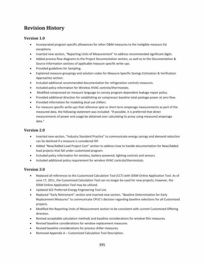
395

Revision History

Version 1.0 • Incorporated program specific allowances for other O&M measures to the ineligible measure list

exceptions.

• Inserted new section, “Reporting Units of Measurement” to address recommended significant digits.

• Added process flow diagrams to the Project Documentation section, as well as to the Documentation & Source Information sections of applicable measure specific write-ups.

• Provided guidelines for Sampling.

• Explained measure groupings and solution codes for Measure Specific Savings Estimation & Verification Approaches section.

• Included additional recommended documentation for refrigeration controls measures.

• Included policy information for Wireless HVAC controls/thermostats.

• Modified compressed air measure language to convey program dependent leakage repair policy.

• Provided additional direction for establishing air compressor baseline total package power at zero flow.

• Provided information for modeling dual use chillers.

• For measure specific write-ups that reference spot or short term amperage measurements as part of the measured data, the following statement was included: “If possible, it is preferred that direct measurements of power and usage be obtained over calculating its proxy using measured amperage data.”

Version 2.0 • Inserted new section, “Industry Standard Practice” to communicate energy savings and demand reduction

can be declined if a measure is considered ISP.

• Added “New/Added Load Project Cost” section to address how to handle documentation for New/Added load projects that fall under customized program.

• Included policy information for wireless, battery-powered, lighting controls and sensors.

• Included additional policy requirement for wireless HVAC controls/thermostats.

Version 3.0 • Replaced all references to the Customized Calculation Tool (CCT) with IDSM Online Application Tool. As of

June 17, 2011, the Customized Calculation Tool can no longer be used for new projects; however, the IDSM Online Application Tool may be utilized.

• Updated SCE Preferred Energy Engineering Tool List.

• Replaced “Early Retirement” section and inserted new section, “Baseline Determination for Early Replacement Measures” to communicate CPUC’s decision regarding baseline selections for all Customized projects.

• Modified the Reporting Units of Measurement section to be consistent with current Customized Offering direction.

• Revised acceptable calculation methods and baseline considerations for window film measures.

• Revised baseline considerations for window replacement measures.

• Revised baseline considerations for process chiller measures.

• Removed Appendix A – Customized Calculation Tool Description.

396

Version 4.0 • Added section for establishing retrofit type and expanded on descriptions for measure categories (ROB,

NEW, REA, RET).

• Removed references to right sizing, which is only eligible under the RCx program.

• Revised Project Cost Documentation section to address CPUC dual baseline decision; describes how to calculate measure costs for ROB, NEW, REA, RET baseline 1 and RET baseline 2.

• Addressed how to determine baseline energy performance for four replacement scenarios in the HVAC – Chillers and Process – Chillers sections. Provided detailed information for the following replacements: water-cooled to air-cooled, air-cooled to water-cooled, water-cooled to water-cooled and air-cooled to air-cooled.

• Updated measurement requirements for HVAC – Chillers, HVAC – Frictionless Chiller Retrofits and HVAC – Compressor Retrofits (0-250,000 kWh – seven days, 250,000-1,000,000 kWh – fourteen days, 1,000,000+ kWh – one month, although one month in summer and another month in winter is preferred).

• Corrected solution code for Pumping – Controls POCs for Oil Wells from PM-709320 to PM-70932.

• Clarified Measured Data Requirements for Process – Fans.

• Page 27 – Added details of the Three-Prong Test for Fuel Substitution Measures.

• Changed verbiage for “Air-cooled to Water-cooled Chiller, Scenario 2” on page 174.

• “Post Install Project Cost” section on page 52 - Clarified that all claimed project costs must be justified.

Version 4.1 • Included description of the three prong test for fuel switching measures.

• Specified guidelines for documenting internal labor costs.

• Documented new policy for calculating interactive effects for lighting replacement measures.

• Modified baseline 1 for the RET of an air-cooled chiller over 300 tons for HVAC – Chiller and Process – Chiller measure specific sections.

• Updated HVAC – Frictionless Chiller Retrofits section.

• Added language, where appropriate, to address measure specific baseline considerations for dual baselines.

Version 4.2 • Updated Preferred Tool List - Version 12.0.

• Specified that calculations should be submitted using a dual baseline approach for projects involving RET- early retirement measures.

• Provided RUL calculation methods.

• Clarified RET applicability for existing equipment that has exhausted DEER EUL.

• Expanded on Install/Program Type Energy Savings.

• Included description of required documentation for retrofits that trigger energy efficiency or general codes and standards.

• Updated project cost documentation section per EAS’ Measure Cost rev7.docx.

Version 5.0 • Updated project cost documentation section per EAS’ Dual Baseline and Interactive Effects Presentation

4-24-12.

• Clarified EUL for Retrofit Add-on Measures.

397

• Expanded Project Documentation section to specifically include requirements for occupancy sensor and day-lighting controls.

• Updated measure data requirements for high efficiency injection molding machine upgrades.

• Added new measure specific section to address motor controller measures.

• Updated preferred tool list to include PTAC Occupancy Sensor Calculation Tool (POST).

• Documented appropriate use of POST for PTAC occupancy sensor installations.

Version 6.0 • Additional clarification has been provided in the Ineligible Measures list for the three-prong test (pg. 25)

and self-generation or cogeneration projects (pg.26).

• Incremental cost guidance has been included in the Preferred Measure Pre-Install Documentation for Project Costs section (pg. 52) to address special circumstances where it not feasible to calculate incremental cost using standard methods.

• Effective February 15, 2013, the CPUC’s Energy Division imposed new requirements for lighting occupancy sensor projects. The approved approaches for calculating savings have been outlined in the Lighting Controls – Occupancy Sensors measure specific section (pg. 90).

• For compressed air system upgrades, information has been added to the Process – Compressed Air measure specific section (pg. 293) to address situations where CAGI performance data is not available.

• Effective July 1, 2014, the revision number has changed back to version 6.0 to be consistent with all appendices tied to the Customized Calculated Savings Guidelines.

Version 7.0 • Effective March 20, 2013, energy simulation models must be properly calibrated to gas and electric utility

bills to ensure that the gas interactions are taken into account. Additional clarification has been included in the Energy Savings Estimation Approaches section for Calibrated Simulations (pg. 16).

• High Efficiency Transformers and limestone addition to cement grinding process have been added to the list of Ineligible Measures (pg. 27)

• Details have been provided for regressive baselines (pg. 37).

• Baseline consideration clarification added to lighting retrofit projects where the existing illumination is below acceptable levels and the proposed measure improves illumination levels.

• Effective April 30, 2013, Energy Division established new pump control baselines for new construction projects in the oil well industry. The established Industry Standard Practice baselines have been outlines in the Industry Standard Practice section (pg. 40).

• DEER Peak Reduction clarification has been added to the Measured Data and Simulated/Modeled Data Types (pg. 44)

• For occupancy sensor measures, clarification has been added to the first approach for calculating energy savings in the measure specific section Lighting Controls – Occupancy Sensors (pg. 101). This modification provides improved clarification on the approach, but does not change the existing requirements for calculating savings.

• A new measure specific section to address battery charger measures has been included (pg. 295).

• Effective March 31, 2013, traditional fixed-speed hydraulic injection molding machines (IMM) are no longer be accepted as the standard baseline for IMM installations for new/added load or normal replacement projects. The approved Industry Standard Practice baselines for calculating savings have been outlined in the Process – Injection Molding Machine measure specific section (pg. 327).

398

Version 8.0 • Energy Division provided clarification to the existing policy for LED T8 Tubes. Based upon review of the

benefits and limitations of LED tubes, SCE’s policy remains that LED lamps replacing T5/T8 (linear fluorescents) or HID lamps do not qualify for deemed or customized incentives at this time (pg. 27).

• Clarification has been provided for regressive baselines (pg. 38).

• Document options and the corresponding required documents have been outlined for Calculated interior luminaire/fixture lighting retrofit projects in Project Documentation section (pg. 53).

• Redundant equipment cost policy has been addressed in the Project Cost Documentation section (pg. 56).

• Energy savings calculation requirements for applicable measure specific sections have been revised to include lighting power density calculations and coincident diversity factor for Calculated interior luminaire/fixture lighting retrofit projects.

• A definition of LED retrofit kits has been added in the LED measure specific section under special requirements (pg. 101).

• An explanation has been provided as to why 3-way to 2-way valve conversion is not eligible under the Customized Program for any retrofit type (pg. 265).

• For pump measures in the oil field industry claiming 8,760 operation, a 98% adjustment factor must be applied to the operating hours (pg. 305).

• For efficient battery charger projects less than 250,000 kWh, the acceptable calculation methods were modified to indicate that monitored data OR engineering spreadsheet calculations are acceptable (pg. 309).

• Program eligibility has been clarified for industrial blower additions to compressed air systems with VFDs (pg. 323).

• Injection molding machine baseline requirements have been updated in the measure specific section to include an “All Other” category. Average specific energy usage by machine types has been provided (pg. 344).

Version 9.0 • Carbon Absorption Vapor Recovery Systems (VRS) were added to the list of ineligible measures (pg. 27).

• Clarification was provided that equipment or system retrofit must guarantee energy savings for the effective useful life of the product OR for a period of five years, whichever is less. Additionally, a measure that was previously incented by SCE can be removed prior to 5 years (or product EUL) as long as it is replaced with more efficient equipment (pg. 29).

• Additional guidance has been included on how to show SCE influence for non-RET measures and preponderance of evidence for RET measure (pg. 34).

• The standard calculation for projects involving changes in production has been modified (pg. 40).

• Industry Standard Practice Regulatory Background and Guiding Principles have been added (pg. 42)

• M&V costs were identified as an eligible project cost for Custom measures (pg. 59).

• The description for eligible de-lamping measures was broadened to encompass all scenarios in which de-lamping savings can be claimed (pg. 80).

• Enclosed parking garages were defined as interior lighting spaces, in which lighting power density calculations are required (included in lighting measure specific sections).

• Dimming Technologies for HID fixtures was deemed eligible for custom incentive (pg. 89).

• Calculated projects must use the CFL interactive effects and CDF (in lieu of non-CFL) for the LED screw in lamps (pg. 105).

399

• Guidelines were provided to establish a more appropriate equation to estimate savings associated with fan and pump projects using the affinity laws (included in pump and fan measure specific sections).

• Definitions for major and minor oil producers have been provided (pg. 318).

• Clarification has been provided that no feedback loop or lockdown is necessary to be eligible for VFD incentives (pg. 380).