Customer Capital, Financial Constraints,

and Stock Returns

Winston Wei Dou Yan Ji David Reibstein Wei Wu∗

February 7, 2019

Abstract

We develop a model in which customer capital depends on key talents’ contribution

and pure brand recognition. Customer capital guarantees stable demand but is fragile

to financial constraints risk if retained mainly by talents, who tend to escape financially

constrained firms, thus damaging customer capital. Using a proprietary, granular

brand-perception survey, we construct a measure of the firm-level inalienability of

customer capital (ICC) that reflects the degree to which customer capital depends on

talents. Firms with higher ICC have higher average returns, higher talent turnover,

and more precautionary financial policies. The ICC-sorted long-short portfolio’s

return comoves with the financial-constraints-risk factor.

Keywords: Brand loyalty; Financial constraints risk; Inalienable human capital; Talent

turnover. (JEL: G12, G30, M31, M37, E22)

∗Dou: University of Pennsylvania (wdou@wharton.upenn.edu). Ji: HKUST (jiy@ust.hk). Reibstein:University of Pennsylvania (reibstein@wharton.upenn.edu). Wu: Texas A&M (wwu@mays.tamu.edu). Wethank Hengjie Ai, Markus Baldauf, Frederico Belo, Alex Belyakov (AFBC discussant), Christa Bouwman,Adrian Buss, Jeffrey Cai, Zhanhui Chen, Will Diamond, Lukasz Drozd, Bernard Dumas, Paolo Fulghieri,Alexandre Garel, Lorenzo Garlappi, Ron Giammarino, Stefano Giglio, Vincent Glode, Itay Goldstein, NaveenGondhi, Francois Gourio, Jillian Grennan, Po-Hsuan Hsu, Shiyang Huang (discussant), Chuan-Yang Hwang,Don Keim, Leonid Kogan, Adam Kolasinski, Doron Levit, Dongmei Li, Kai Li, Xiaoji Lin, Asaf Manela,Neil Morgan, Christian Opp, Pascal Maenhout, Hernan Ortiz-Molina, Carolin Pflueger, Yue Qiu (CFEAdiscussant), Adriano Rampini, Nick Roussanov, Leena Rudanko (AFA discussant), Alp Simsek, BrunoSolnik, Rob Stambaugh, Roberto Steri (EFA discussant), Sheridan Titman, Kumar Venkataraman, JessicaWachter, Neng Wang, James Weston, Toni Whited, Wei Xiong, Yu Xu, Jialin Yu, Morad Zekhnini (NFAdiscussant), Lu Zhang, Bart Zhou, John Zhu, as well as seminar participants at HKU, HKUST, INSEAD,NTU, Philadelphia Fed, SMU, Texas A&M, UBC, Wharton, AFA, EFA, CFEA, NFA, Rising Five-StarWorkshop at Columbia, AMA for their comments. We also thank John Gerzema, Anna Blender, and DamiRosanwo of the BAV Group for sharing the data, and Ed Lebar and Alina Sorescu for the guidance ondata processing. We thank Dian Yuan, Haowen Dong, and Hezel Gadzikwa for their excellent researchassistance. Winston Dou is especially grateful for the financial support of the Rodney L. White Center forFinancial Research.

1 Introduction

Customer capital – customers’ brand loyalty to the firm – is one of the firm’s most crucialintangible assets, as it determines the capacity of stable demand flows by creating entrybarriers and durable advantages over competitors (see, e.g., Bronnenberg, Dubé andGentzkow, 2012). Developing and sustaining customer capital is essential for a firm’ssurvival, growth, profitability, and ultimately its valuation, even though customer capitaldoes not explicitly appear on the balance sheet.1

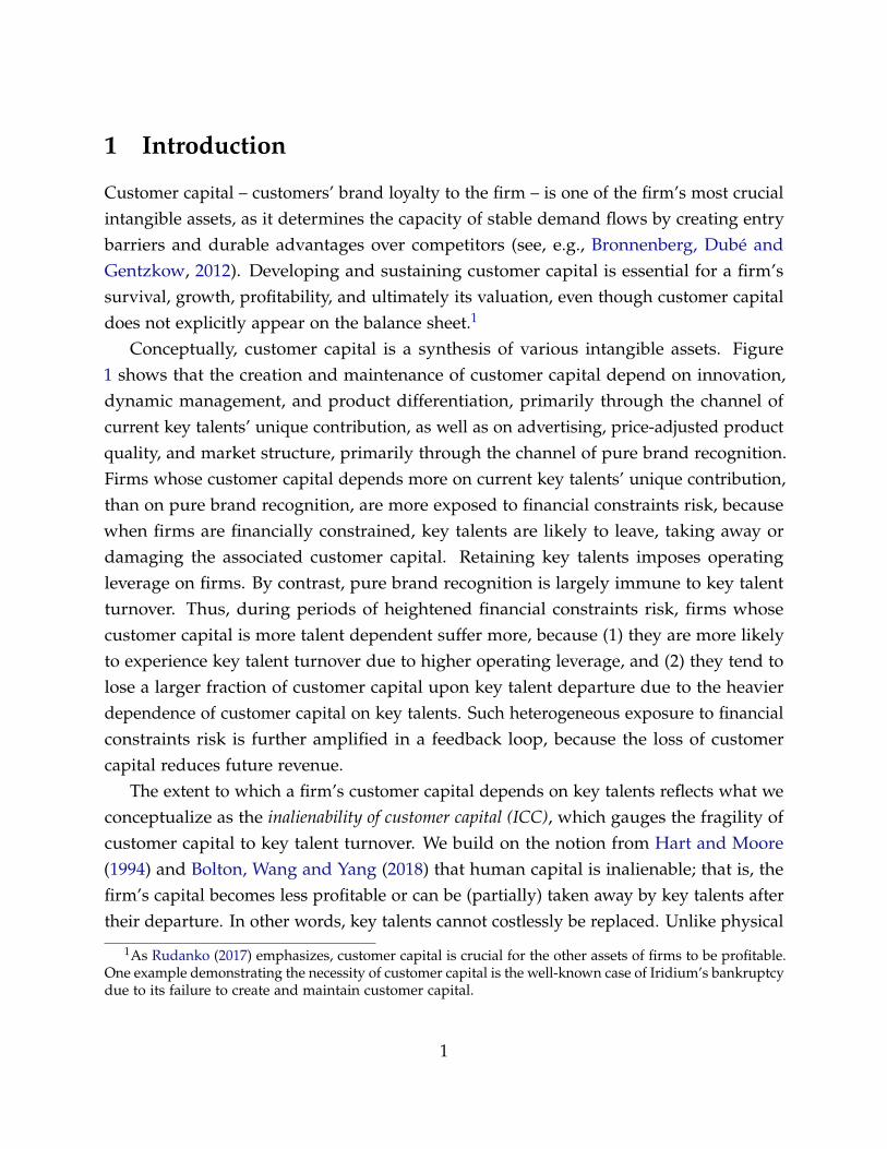
Conceptually, customer capital is a synthesis of various intangible assets. Figure1 shows that the creation and maintenance of customer capital depend on innovation,dynamic management, and product differentiation, primarily through the channel ofcurrent key talents’ unique contribution, as well as on advertising, price-adjusted productquality, and market structure, primarily through the channel of pure brand recognition.Firms whose customer capital depends more on current key talents’ unique contribution,than on pure brand recognition, are more exposed to financial constraints risk, becausewhen firms are financially constrained, key talents are likely to leave, taking away ordamaging the associated customer capital. Retaining key talents imposes operatingleverage on firms. By contrast, pure brand recognition is largely immune to key talentturnover. Thus, during periods of heightened financial constraints risk, firms whosecustomer capital is more talent dependent suffer more, because (1) they are more likelyto experience key talent turnover due to higher operating leverage, and (2) they tend tolose a larger fraction of customer capital upon key talent departure due to the heavierdependence of customer capital on key talents. Such heterogeneous exposure to financialconstraints risk is further amplified in a feedback loop, because the loss of customercapital reduces future revenue.

The extent to which a firm’s customer capital depends on key talents reflects what weconceptualize as the inalienability of customer capital (ICC), which gauges the fragility ofcustomer capital to key talent turnover. We build on the notion from Hart and Moore(1994) and Bolton, Wang and Yang (2018) that human capital is inalienable; that is, thefirm’s capital becomes less profitable or can be (partially) taken away by key talents aftertheir departure. In other words, key talents cannot costlessly be replaced. Unlike physical

1As Rudanko (2017) emphasizes, customer capital is crucial for the other assets of firms to be profitable.One example demonstrating the necessity of customer capital is the well-known case of Iridium’s bankruptcydue to its failure to create and maintain customer capital.

1

InnovationDynamic

ManagementAdvertising

Price-Adjusted Quality

Current Key Talents’ Contribution Pure Brand Recognition

Customer Capital

ProductDifferentiation

Market Structure

Note: The solid arrows represent primary channels, whereas the dashed arrows represent secondary channels.

Figure 1: Different channels of creating and maintaining customer capital

or some other types of intangible capital of the firm such as patents, customer capital thatrelies heavily upon the unique contribution of current key talents can be taken away orseriously damaged by key talents’ departure due to limited legal enforceability. Therefore,the ICC can be viewed as one concrete and important example of the inalienability ofhuman capital.2

Our major contribution lies in examining how the ICC interacts with financial con-straints and investigating the asset pricing implications of this interaction. Like Whitedand Wu (2006) and Buehlmaier and Whited (2018), we focus on the aggregate financial-constraints-risk shock that alters the marginal value of internal funds of all firms si-multaneously. The financial-constraints-risk shock can be jointly driven by multiplemore primitive macroeconomic shocks such as the TFP shock, the uncertainty shock, thefinancing-cost shock, and so on. This shock is shown to carry a negative market price ofrisk (see, e.g., Whited and Wu, 2006; Buehlmaier and Whited, 2018). As the main theoreti-cal contribution, we show that a firm’s exposure to financial-constraints-risk shocks issimultaneously reflected in two cross sections: firms have higher liquidity-driven talentturnover and higher average returns, if (1) their customer capital is more talent dependent,and (2) they are more financially constrained. The cross-equation restrictions implied bythe model predictions on both turnover and returns in the two cross sections over-identify

2The ICC is also linked to other types of inalienable capital associated with key talents, such as theirsocial capital (see, e.g., Arrow, 1999; Glaeser et al., 1999; Durlauf, 2002; Sobel, 2002; Durlauf and Fafchamps,2005).

2

the same asset pricing factor, the financial-constraints-risk factor, which makes our modelmore quantitatively disciplined. The empirical analyses rely upon measuring the ICC,which is challenging. As the main empirical contribution, we introduce a measure for theICC, based on a proprietary, granular brand perception survey database. We also provideempirical evidence that strongly supports the theoretical implications.

We start by developing a baseline dynamic model to illustrate the key underlyingmechanism. In the baseline model, the firm’s external financing is costly, which motivatesretained earnings and imposes financial constraints risk on itself. The marginal value of itsinternal funds is determined jointly by the endogenous level of firm-specific cash holdingsand the exogenous level of financial constraints risk. The latter is time-varying and drivenby an aggregate shock. Such a shock is referred to as the financial-constraints-risk shockand is the only systematic shock in the baseline model. Customer capital guaranteesstable demand flows and is partly maintained by key talents. The contract between keytalents and shareholders features two-sided limited commitment. On the one hand, keytalents have outside options and limited commitment to the firm; as a result, maintainingtalent-dependent customer capital requires that firms compensate key talents and thusimposes operating leverage on the firm. On the other hand, shareholders would chooseto let key talents go if retaining them becomes too costly. Thus, heterogeneous levels ofICC lead to firms’ differential exposure to the aggregate financial-constraints-risk shock,which simultaneously generates the spreads in (risk-adjusted) average stock returns andtalent turnover rates.

More precisely, shareholders face the intertemporal trade-off between risks and returnswhen they decide whether or not to retain talent-dependent customer capital. Althoughretaining talent-dependent customer capital on average brings positive net cash flows,the associated operating leverage increases firms’ exposure to financial constraints risk.When firms face heightened financial constraints risk, key talents may find it optimalto escape from a sinking ship or jump to a safer boat (see, e.g., Brown and Matsa, 2016;Babina, 2017; Baghai et al., 2017).3 Alternatively, firms may find it optimal to conductoperating deleveraging by replacing incumbent talents with less-cash-compensated newtalents (see, e.g., Gilson and Vetsuypens, 1993). Thus, customer capital is robust against

3Babina (2017) provides several pieces of evidence consistent with our model’s implications. First,employees’ exit rates are higher in distressed firms. Second, employees exiting distressed firms earn higherwages prior to the exit than employees exiting non-distressed firms. Third, the exit rate of employees fromdistressed firms is greater in the states with weaker enforcement of non-compete agreements.

3

financial constraints risk if it depends mainly on customers’ pure brand recognition.By contrast, customer capital is fragile to financial constraints risk if it depends mainlyon the contribution of current key talents, because the effective cost of compensationincreases with the marginal value of internal funds of the firm. Equilibrium liquidity-driven separation and turnover due to financial constraints, which is commonly observedin the data, is the key to our model’s mechanism. By contrast, in standard models ofinalienable human capital, such as those of Hart and Moore (1994), Lustig, Syverson andNieuwerburgh (2011), Eisfeldt and Papanikolaou (2013), and Bolton, Wang and Yang(2018), there is no separation in equilibrium.

After illustrating the key mechanisms using the baseline model, we formally test themodel’s empirical implications. The main empirical challenge lies in finding high-qualitydata on consumers’ brand loyalty and its talent dependence measured in a consistent wayacross firms. We tackle this challenge by constructing a measure for the degree to whichcustomer capital depends on talents, based on a proprietary, granular brand perceptionsurvey database. The database, provided by the BAV Group, is regarded as the world’smost comprehensive database of consumer brand perception.

The talent dependence of customer capital is reflected by the extent to which brandloyalty is associated with the firm’s key talents. The BAV consumer survey data directlyquantify a firm’s general brand loyalty and its specific components. Particularly, the BAVGroup has developed two major brand metrics: brand stature and brand strength. Brandstature quantifies a firm’s general brand loyalty, whereas brand strength quantifies a firm’sbrand loyalty specifically associated with key talents, mainly through the innovativenessand distinctiveness of the products as well as the efficiency of the management team. Thus,we use the ratio of the two as an empirical measure for the talent dependence of customercapital (i.e., the ICC). We emphasize that although the ICC can endogenously affect theextent to which a firm is financially constrained (i.e., the marginal value of internal funds),our survey-based ICC measure is not designed to be one of those empirical measures forfinancial constraints like the ones developed by Whited and Wu (2006) and Buehlmaierand Whited (2018). Those measures capture essentially different economic concepts.

To justify the connection between our survey-based ICC measure and its counterpart inthe model, the talent dependence of customer capital, we need to show that the empiricalICC measure is able to capture the three major properties of its theoretical counterpartin our model. The three properties are that (1) firms whose talents play relatively moreimportant roles are associated with higher ICC; (2) firms with higher ICC tend to lose a

4

larger fraction of customer capital upon talent turnover; and (3) firms’ customer capitalbecomes less talent dependent (i.e., the ICC declines) upon talent turnover. Followingthe methodology of external validation tests in the work of Bloom and Reenen (2007),we provide direct evidence that our survey-based ICC measure satisfies all of the threeaforementioned properties.

We present two main sets of empirical results to support our model. The first setshows that the patterns of cross-sectional stock returns based on ICC levels are consistentwith our model’s implications. The second set shows that the patterns of cross-sectionaltalent turnover based on ICC levels support our model’s main mechanism.

Regarding the first set of empirical results, we show that firms with higher ICChave higher average (risk-adjusted) excess returns. The ICC spread is persistent aroundthe time of portfolio formation and is robust after controlling for various measures ofcustomer capital, intangible assets, and industry classifications. Moreover, the ICC spreadremains significantly positive after controlling for R&D measures using Fama-MacBethregressions. By extending our sample to all U.S. public firms, we show that the ICCspread is an asset pricing factor, which is referred to as the c-factor. We further show thatthe c-factor is highly correlated with the financial-constraints-risk factor constructed basedon the two financial constraints measures of Whited and Wu (2006) and Buehlmaier andWhited (2018), suggesting that the c-factor also captures the same financial constraintsrisk to a large extent. The strong comovement between the c-factor and the financial-constraints-risk factor convincingly supports the main channel of our theory — theinteraction between the ICC and financial constraints.

Regarding the second set of empirical results, we show that firms with higher ICC areassociated with higher talent turnover rates, a finding that is robust for both executivesand innovators. Moreover, the positive relation between the ICC and the talent turnoverrate is more pronounced in the periods of heightened financial constraints risk and in thestates where the enforcement of non-compete agreements is weaker.

Finally, we extend the baseline model to a richer model with three additional ingre-dients for quantitative analysis. The first is the aggregate productivity shock to allowmultiple asset pricing factors in the model; the second is the firm-specific shock to theICC to match a more realistic cross-sectional distribution of talent compensation in thedata; and the third is the non-pecuniary private benefits to the key talents who work forthe firms with prestigious brands. Using the calibrated extended model, we show thatthe interaction between the ICC and financial constraints determines firms’ exposure to

5

the aggregate financial-constraints-risk shock, which can quantitatively explain the jointpatterns in talent turnover and stock returns. The calibrated extended model also allowsus to investigate the economic importance of each mechanism in the model. Accordingto the quantitative analysis, the interaction between the ICC and financial constraintsis crucial for generating the differential exposure to financial constraints risk. Missingeither the ICC or financial constraints makes it impossible for the model and the data toreconcile.

Related Literature. Our paper is related to the large literature on cross-sectional stockreturns (see, e.g., Cochrane, 1991; Berk, Green and Naik, 1999; Gomes, Kogan and Zhang,2003; Nagel, 2005; Zhang, 2005; Livdan, Sapriza and Zhang, 2009; Belo and Lin, 2012;Eisfeldt and Papanikolaou, 2013; Ai and Kiku, 2013; Ai, Croce and Li, 2013; Belo, Lin andBazdresch, 2014; Kogan and Papanikolaou, 2014; Kumar and Li, 2016; Belo et al., 2017;Hirshleifer, Hsu and Li, 2017). Nagel (2013) provides a comprehensive survey. Unlike mostpapers in this literature, we study the asset pricing implications in a dynamic corporatefinance model with financial constraints. Indeed, research on cross-sectional asset pricinghas been increasingly emphasizing the importance of financial constraints and corporateliquidity (see, e.g., Whited and Wu, 2006; Campbell, Hilscher and Szilagyi, 2008; Garlappi,Shu and Yan, 2008; Gomes and Schmid, 2010; Garlappi and Yan, 2011; Li, 2011; Ai et al.,2017; Buehlmaier and Whited, 2018). This increase is due to the empirical evidenceshowing that cash holdings are often large, and a more important reason is that corporateliquidity (or cash) arises naturally as an inevitable state variable in dynamic corporatefinance models with financial constraints. This idea is not yet as well appreciated inthe asset pricing literature as it perhaps should be. We contribute to the literature byshedding light on firms’ heterogeneous exposure to financial-constraints-risk shocksthrough their different ICC. Moreover, our model generates asset pricing implications offinancial-constraints-risk shocks in two different cross sections simultaneously.

Our paper also contributes to the emerging literature on the interaction between cus-tomer capital and finance. Titman (1984) and Titman and Wessels (1988) provide the firstpiece of theoretical insight into and empirical evidence on the interaction between firms’financial and product market characteristics. In this literature, a large body of researchexamines how financial characteristics influence firms’ performance and decisions in theproduct market (see, e.g., Chevalier and Scharfstein, 1996; Fresard, 2010; Phillips andSertsios, 2013; Gourio and Rudanko, 2014; Gilchrist et al., 2017; D’Acunto et al., 2018),

6

whereas only a few papers focus on the implication of product market characteristicson valuation and various corporate policies (see, e.g., Dumas, 1989; Banerjee, Dasguptaand Kim, 2008; Larkin, 2013; Belo, Lin and Vitorino, 2014; Gourio and Rudanko, 2014;Vitorino, 2014; Dou and Ji, 2017; Belo et al., 2018). We depart from the existing literatureby investigating the financial implications of the ICC.

Our paper is also related to the literature on inalienable human capital dating backto Hart and Moore (1994). Human capital is embodied in a firm’s key talents, who havethe option to walk away. Thus, shareholders are exposed to the risk inherent in thelimited commitment of key talents. The talent-dependent customer capital we investigateprovides one of the most concrete and convincing examples of inalienable human capital.Lustig, Syverson and Nieuwerburgh (2011) develop a model with optimal compensationto managers who cannot commit to staying with the firm. Eisfeldt and Papanikolaou(2013) show that the firms with more organization capital are riskier, due to their greaterexposure to technology frontier shocks. Berk, Stanton and Zechner (2010) develop a modelwith entrenched employees under long-term optimal labor contracts to analyze theirimplications on the optimal capital structure. Their model focuses on entrenched workerswho cannot be fired by firms and are thus overpaid. Our theory is related to the workof Bolton, Wang and Yang (2018), who analyze the implications of inalienable humancapital on corporate credit limits, talents’ idiosyncratic risk exposure, and liquidity andrisk management, in a standard long-term optimal contracting framework. Our modeldoes not focus on those implications. Instead, we highlight the operating leverage effectimposed by the ICC in models with financial constraints and discuss its asset pricingimplications.4

The inalienability of human capital is essentially caused by limited commitment. Ourpaper is also related to the optimal contracting problem with limited commitment (see,e.g., Alvarez and Jermann, 2000, 2001; Albuquerque and Hopenhayn, 2004; Rampiniand Viswanathan, 2013; Ai and Bhandari, 2018; Ai and Li, 2015; Bolton, Wang andYang, 2018). Several papers in this literature study the asset pricing implications oflimited commitment. For example, Alvarez and Jermann (2000, 2001) study its assetpricing implications in an incomplete market model with one-sided limited commitment.

4Eisfeldt and Rampini (2008) also propose a model of talent turnover. Their model is different from oursin two ways. First, in their model, managers are compensated due to a moral hazard problem. Second,they focus on the aggregate turnover patterns over the business cycle instead of the cross-sectional turnoverpatterns. Extending our model to a general equilibrium framework to analyze aggregate turnover is aninteresting direction for future research.

7

Recently, Ai and Bhandari (2018) provide a unified view of labor market risk and assetprice through a general equilibrium model with two-sided limited commitment andmoral hazard. Our paper is particularly related to Ai and Bhandari (2018) because bothpapers emphasize that firms offering larger labor compensation effectively bear higheroperating leverage, which generates cross-sectional asset pricing implications. Our modeladopts a different angle, however, by emphasizing compensation to key talents due tothe ICC. Moreover, we show that the presence of financial constraints risk amplifies theoperating leverage channel, generating significant asset pricing implications in the crosssection.

Finally, our paper is related to the growing literature on the intersection of marketingand finance. The BAV survey database is the standard data source for measuring brandvalue (see, e.g., Gerzema and Lebar, 2008; Keller, 2008; Mizik and Jacobson, 2008; Aaker,2012; Lovett, Peres and Shachar, 2014; Tavassoli, Sorescu and Chandy, 2014). Our studyadds to this strand of literature by dissecting the channels of maintaining customer capitaland providing new implications of customer capital on asset prices and talent turnover.

2 Baseline Model

We develop an asset pricing model of heterogeneous firms to explain the interactionbetween the ICC and financial constraints, as well as its role in determining the jointpatterns of asset pricing and talent turnover. Importantly, we show that the heterogeneousexposure to aggregate financial-constraints-risk shocks is simultaneously reflected intwo different cross sections — the ICC and the extent to which firms are financiallyconstrained.

2.1 Basic Environment

Firms and Agents. A continuum of firms and agents exist in the economy. Agents fundfirms by holding equity as shareholders and purchase firms’ goods as consumers. Someagents also act as talents who manage firms. We assume that agents can trade a completeset of contingent claims on consumption, and a representative agent owns the equity andconsumes the goods of all firms. The representative agent is only exposed to aggregateshocks. We omit the firm subscript for simplicity.

8

Production. All firms have the same AK production technology with productivity ea,and they produce a flow of goods over [t, t + dt] with intensity

Yt = eaKt, (2.1)

where physical capital Kt is rented from a capital rental market at the competitive rentalrate r + δK. Here, r is the risk-free rate and δK is the rate of physical capital depreciation.To keep the model manageable, we assume away physical capital adjustment costs andassume that firms can only rent physical capital. In fact, assuming that firms producegoods using rental capital is a standard modeling technique in the macroeconomicsliterature (see, e.g., Jorgenson, 1963; Buera and Shin, 2013; Moll, 2014) and in the corporatetheory literature (see, e.g., Rampini and Viswanathan, 2013).

Instantaneous demand capacity Btdt over [t, t + dt] depends on the firm’s customercapital Bt, which can be thought of as a measure of the firm’s existing customer base attime t. The amount of goods sold by the firm is Stdt over [t, t + dt], where we requireSt ≤ Yt and St ≤ Bt, capturing the fact that total sales cannot exceed production output Yt

or the demand capacity Bt as in Gourio and Rudanko (2014). In the equilibrium, the salesare equal to St = min(Yt, Bt). This does not mean that customer capital Bt is a productioninput or the production technology is Leontief. The production technology is still AKwith physical capital Kt as the only input. The Leontief functional form captures onlythe fact that the equilibrium sales cannot exceed the smaller value between consumerdemand and the firm’s production.

Under our benchmark calibration in which r + δK < ea, it is optimal for the firmto produce and match demand capacities by employing physical capital Kt = Bt/ea.Thus, all firms produce and sell all of the outputs up to the short-run demand capacitySt = Yt = Bt, and the firm size is essentially determined by the firm’s customer capital Bt.As will be shown in Section 2.4, by exploiting the homogeneity of Bt, we can reduce thedimensionality of the firm’s optimization problem. This modeling approach is inspiredby Bolton, Chen and Wang (2011), who exploit the homogeneity of firm size, measuredby physical capital Kt in their model.

Customer Capital Growth. The firm hires it sales representatives to build new customercapital at convex costs φ(it)Btdt over [t, t + dt], with the adjustment cost function being

9

φ(it) = αiηt . The evolution of customer capital Bt is given by

dBt = [µ(it)− δB]Btdt, (2.2)

where δB is the rate of depreciation of customer capital. We assume that5

µ(it) = ψit, (2.3)

implying that the firm can grow customer capital faster by hiring more sales representa-tives. The coefficient ψ captures the effective search-matching efficiency in the productmarket.

External Financial Constraints. We assume that the firm has access to the equitymarket but not the corporate debt market.6 The firm has the option to pay out dividenddDt or issue equity dHt to finance expenses over the next instant dt. The financing costincludes a fixed cost γ proportional to firm size and a variable cost ϕ proportional to theamount of equity issued. That is, the deadweight loss of shareholders for raising fundsW for a firm with customer capital B is

Φ(W; B) ≡ γB︸︷︷︸fixed cost

+ ϕW.︸︷︷︸variable cost

(2.4)

The modelling of fixed and variable equity financing costs follows the literature (see, e.g.,Gomes, 2001; Riddick and Whited, 2009; Gomes and Schmid, 2010; Bolton, Chen andWang, 2011; Eisfeldt and Muir, 2016). The key idea is simple: external funds are notperfect substitutes for internal funds.

Financial constraints motivate the firm to hoard cash Wt on its balance sheet. Holdingcash is costly due to the agency costs associated with free cash in the firm or taxdistortions.7 We assume that the return from cash is the risk-free rate r minus a carrycost ρ > 0. The cash-carrying cost implies that the firm would pay out dividends when

5In Online Appendix A1, we derive (2.3) as the equilibrium representation in a search-matching model.6This assumption is innocuous for our purpose because we focus on the endogenous time-varying

marginal value of internal funds. This simplification captures our theory’s main idea while maintainingtractability.

7The interest earned by the firm on its cash holdings is taxed at the corporate tax rate, which generallyexceeds the personal tax rate on interest income (see, e.g., Graham, 2000; Faulkender and Wang, 2006;Riddick and Whited, 2009).

10

cash holdings Wt are high. In our model, cash holdings capture all internal liquid fundsheld by the firm.

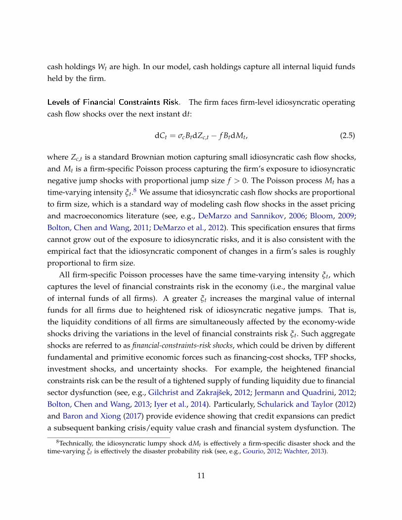
Levels of Financial Constraints Risk. The firm faces firm-level idiosyncratic operatingcash flow shocks over the next instant dt:

dCt = σcBtdZc,t − f BtdMt, (2.5)

where Zc,t is a standard Brownian motion capturing small idiosyncratic cash flow shocks,and Mt is a firm-specific Poisson process capturing the firm’s exposure to idiosyncraticnegative jump shocks with proportional jump size f > 0. The Poisson process Mt has atime-varying intensity ξt.8 We assume that idiosyncratic cash flow shocks are proportionalto firm size, which is a standard way of modeling cash flow shocks in the asset pricingand macroeconomics literature (see, e.g., DeMarzo and Sannikov, 2006; Bloom, 2009;Bolton, Chen and Wang, 2011; DeMarzo et al., 2012). This specification ensures that firmscannot grow out of the exposure to idiosyncratic risks, and it is also consistent with theempirical fact that the idiosyncratic component of changes in a firm’s sales is roughlyproportional to firm size.

All firm-specific Poisson processes have the same time-varying intensity ξt, whichcaptures the level of financial constraints risk in the economy (i.e., the marginal valueof internal funds of all firms). A greater ξt increases the marginal value of internalfunds for all firms due to heightened risk of idiosyncratic negative jumps. That is,the liquidity conditions of all firms are simultaneously affected by the economy-wideshocks driving the variations in the level of financial constraints risk ξt. Such aggregateshocks are referred to as financial-constraints-risk shocks, which could be driven by differentfundamental and primitive economic forces such as financing-cost shocks, TFP shocks,investment shocks, and uncertainty shocks. For example, the heightened financialconstraints risk can be the result of a tightened supply of funding liquidity due to financialsector dysfunction (see, e.g., Gilchrist and Zakrajšek, 2012; Jermann and Quadrini, 2012;Bolton, Chen and Wang, 2013; Iyer et al., 2014). Particularly, Schularick and Taylor (2012)and Baron and Xiong (2017) provide evidence showing that credit expansions can predicta subsequent banking crisis/equity value crash and financial system dysfunction. The

8Technically, the idiosyncratic lumpy shock dMt is effectively a firm-specific disaster shock and thetime-varying ξt is effectively the disaster probability risk (see, e.g., Gourio, 2012; Wachter, 2013).

11

heightened financial constraints risk could also be the result of excessive demand forfunding liquidity, when firms with great investment opportunities are eager to investaggressively (see, e.g., Gomes, Yaron and Zhang, 2006; Riddick and Whited, 2009). Theincentive for making such investments is especially large under the displacement riskimposed by peer innovations (see, e.g., Kogan et al., 2017). To structurally micro-foundour specification of financial-constraints-risk shocks, we develop a simple framework andformally show that primitive economic shocks can endogenously drive fluctuations in themarginal value of internal funds for firms. See Online Appendix A.2 for a more detaileddiscussion.

We focus on investigating the implications of the fluctuations in the marginal valueof their internal funds, without specifying the underlying primitive economic aggregateforces.9 In other words, we take a parsimonious yet generic modeling approach tocapture the random fluctuations in the marginal value of firms’ internal funds. We donot explicitly connect the financial-constraints-risk shock (i.e., the shock to the marginalvalue of internal funds) to any particular primitive shock, because we do not want to givethe false impression that the financial-constraints-risk shock is purely driven by somesingle primitive shock.

In particular, we model financial-constraints-risk shocks by assuming that the intensityξt follows a two-state Markov process, with its value being ξL and ξH, and ξL < ξH.10

The transition intensity from ξL to ξH is q(ξL,ξH), and that from ξH to ξL is q(ξH ,ξL). Theaggregate processes of transitions are denoted by N(ξL,ξH)

t and N(ξH ,ξL)t .

Pricing Kernel. Because the market is complete, only aggregate shocks are priced, andthe only aggregate shock is the financial-constraints-risk shock in the baseline model.We assume that the financial-constraints-risk shock carries a negative market price ofrisk. As discussed above, the financial-constraints-risk shock may well be driven by themore fundamental and primitive economic shocks. The asset pricing literature has shownextensively that those primitive economic shocks are priced by investors. More precisely,the financial-constraints-risk shock should be priced with a negative market price of risk

9The approach we are taking is similar in spirit to that of the Lucas-tree model for studying asset pricing.In the Lucas-tree model, to study asset pricing, shocks to consumption are directly modeled even thoughthey are driven by more fundamental and primitive economic forces.

10The importance of the aggregate shocks driving the variation in risks has been shown in the macroeco-nomics and asset pricing literature (see, e.g., Gourio, 2012; Gourio, Siemer and Verdelhan, 2013; Christiano,Motto and Rostagno, 2014).

12

because it is (1) positively driven by the financial-sector shock (i.e., the financing-costshock), which carries a negative market price of risk; (2) negatively driven by the TFPshock, which carries a positive market price of risk; (3) positively driven by the cash-flowuncertainty shock, which carries a negative market price of risk; and (4) positively drivenby the investment shock, which carries a negative market price of risk. Further, empiricalfindings support the assumption that the financial-constraints-risk shock is negativelypriced by investors (see Whited and Wu, 2006; Buehlmaier and Whited, 2018).

Thus, we assume that the representative agent’s state-price density Λt evolves asfollows:

dΛt

Λt= −rdt + ∑

ξ ′ 6=ξt

[e−κ(ξt ,ξ′) − 1]︸ ︷︷ ︸market price of risk

(dN(ξt,ξ ′)t − q(ξt,ξ ′)dt).︸ ︷︷ ︸

financial-constraints-risk shock

(2.6)

The market price of risk for financial-constraints-risk shocks is constant and exoge-nously specified, captured by κ(ξ,ξ ′). We assume κ(ξL,ξH) < 0, meaning that heightenedfinancial constraints risk raises the state-price density.

2.2 Inalienability of Customer Capital (ICC)

An essential feature of customer capital is its inalienability due to its dependence onkey talents’ human capital, including skills, knowledge, connections, reputation, and soon. Shareholders have the option to fire key talents, and key talents have the option toleave the firm and start their own business.11 We assume that a fraction τt of the firm’scustomer capital Bt can be affected by talent turnover. Thus, τt captures the degree towhich customer capital depends on key talents, and we refer to τtBt as talent-dependentcustomer capital. By definition, τt is the firm’s ICC at time t, because it reflects thefragility of customer capital to key talent turnover.

More precisely, when key talents leave, they take away mτtBt, where the parameter mcaptures the damage ratio of talent-dependent customer capital due to turnover. Uponthe occurrence of turnover over [t, t +dt], the remaining customer capital is (1−mτt)Bt =

Bt−mτBt, among which (1−m)τtBt = τtBt−mτtBt is maintained by key talents. Thus, τt

jumps to (1−m)τt/(1−mτt) immediately after turnover. Assume that the ICC τt ≡ e−ωt

11For simplicity, our contracting framework does not incorporate moral hazard (see, e.g., Holmstrom,1979; Holmstrom and Milgrom, 1987) or managerial short-termism (see, e.g., Stein, 1988, 1989; Shleiferand Vishny, 1990; Bolton, Scheinkman and Xiong, 2006). Evaluating the asset pricing implications of theirinteractions with customer capital is an interesting topic for future research.

13

is mean reverting and ωt follows

dωt = −µω(ωt −ω)dt +[ln(1−me−ωt

)− ln (1−m)

]dJt,︸ ︷︷ ︸

endogenous turnover

(2.7)

where the process Jt is an idiosyncratic Poisson process of the incidences of talent turnover;that is, the Poisson process Jt jumps up by one (dJt = 1) over [t, t + dt] if and only iftalent turnover occurs during [t, t + dt]. Upon turnover, ωt jumps upward over [t, t + dt]with the amount of ln (1−me−ωt)− ln (1−m). Because the endogenous jump is alwayspositive, ωt is always positive, and thus τt ∈ (0, 1).

The ICC is defined following the spirit of the concept of inalienable human capitalcoined by Hart and Moore (1994). In the models of Hart and Moore (1994) and Bolton,Wang and Yang (2018), human capital is inalienable in the sense that, as a productioninput, it cannot be taken away from its possessors (i.e. key talents) due to limited legalenforcement. Also due to limited commitment of key talents, human capital cannot befully collateralized for external financing or fully capitalized by firms for generatingprofits. Specifically, Hart and Moore (1994) assume that physical capital is operated mostefficiently by the original key talents, and its productivity drops when it is operatedby other talents. There is no separation between the firm and the key talent in theequilibrium, because their paper focuses on a deterministic contracting problem. In theirdeterministic model, the optimal debt contract can be achieved by restricting attention to“repudiation-proof” contracts. Their modeling specification of inalienability is essentiallysimilar to ours, but we consider a stochastic model. In the model of Bolton, Wang andYang (2018), human capital of key talents is a necessary input for operating a firm’sphysical capital. If talents leave, physical capital cannot generate any cash flows, and thefirm is terminated. As a result, there is no separation in the equilibrium either. In ourmodel, when key talents leave, a fraction of the firm’s customer capital (which dependson the ICC) is taken away and thus stops generating cash flows for the firm. However,the remaining customer capital in the firm can still generate cash flows, albeit in smalleramounts, because the firm can immediately hire new talents to replace old talents withoutpaying any upfront replacement costs. Therefore, the ICC is fundamentally linked tothe inalienability of human capital. But in some sense, our notion of inalienable humancapital is weaker than that of Bolton, Wang and Yang (2018), which is the key reason ourmodel can allow for endogenous separation between key talents and firms in equilibrium.

14

2.3 Liquidity-Driven Turnover

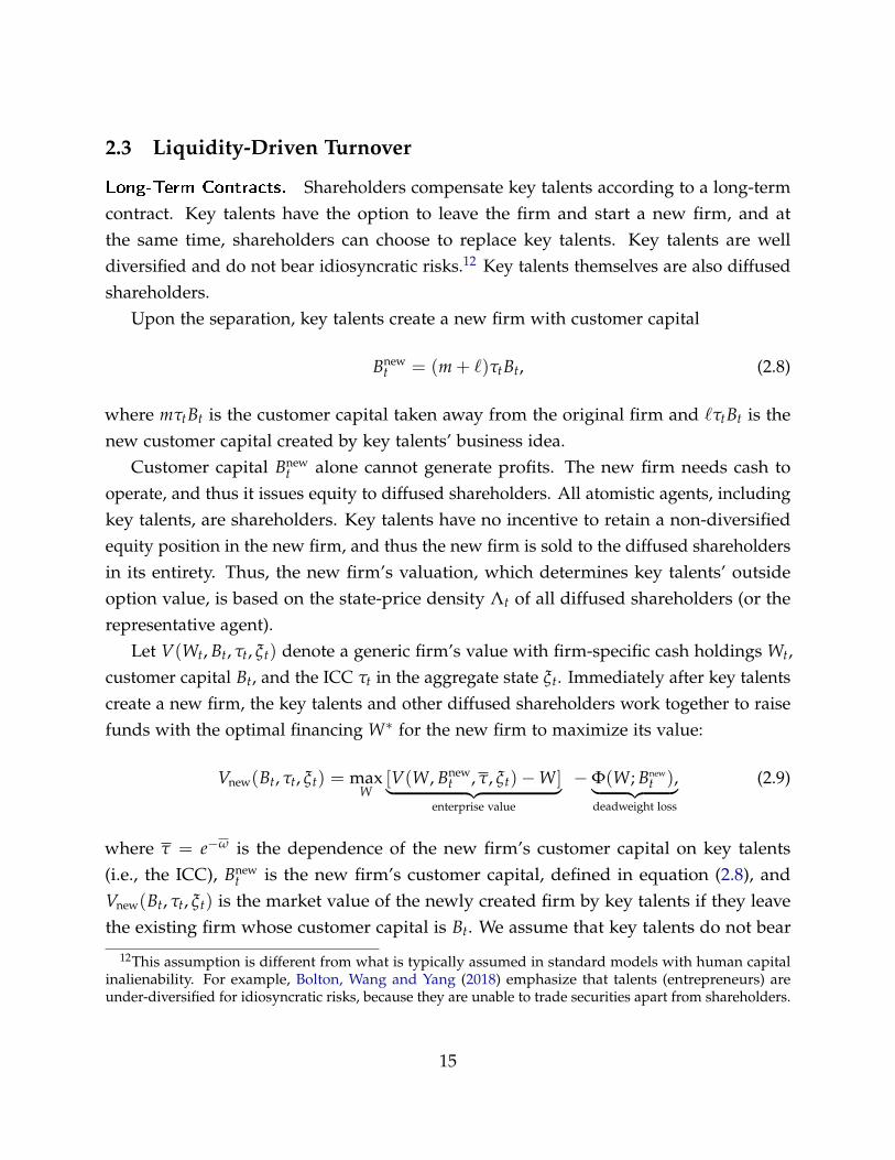
Long-Term Contracts. Shareholders compensate key talents according to a long-termcontract. Key talents have the option to leave the firm and start a new firm, and atthe same time, shareholders can choose to replace key talents. Key talents are welldiversified and do not bear idiosyncratic risks.12 Key talents themselves are also diffusedshareholders.

Upon the separation, key talents create a new firm with customer capital

Bnewt = (m + `)τtBt, (2.8)

where mτtBt is the customer capital taken away from the original firm and `τtBt is thenew customer capital created by key talents’ business idea.

Customer capital Bnewt alone cannot generate profits. The new firm needs cash to

operate, and thus it issues equity to diffused shareholders. All atomistic agents, includingkey talents, are shareholders. Key talents have no incentive to retain a non-diversifiedequity position in the new firm, and thus the new firm is sold to the diffused shareholdersin its entirety. Thus, the new firm’s valuation, which determines key talents’ outsideoption value, is based on the state-price density Λt of all diffused shareholders (or therepresentative agent).

Let V(Wt, Bt, τt, ξt) denote a generic firm’s value with firm-specific cash holdings Wt,customer capital Bt, and the ICC τt in the aggregate state ξt. Immediately after key talentscreate a new firm, the key talents and other diffused shareholders work together to raisefunds with the optimal financing W∗ for the new firm to maximize its value:

Vnew(Bt, τt, ξt) = maxW

[V(W, Bnewt , τ, ξt)−W]︸ ︷︷ ︸

enterprise value

−Φ(W; Bnewt ),︸ ︷︷ ︸

deadweight loss

(2.9)

where τ = e−ω is the dependence of the new firm’s customer capital on key talents(i.e., the ICC), Bnew

t is the new firm’s customer capital, defined in equation (2.8), andVnew(Bt, τt, ξt) is the market value of the newly created firm by key talents if they leavethe existing firm whose customer capital is Bt. We assume that key talents do not bear

12This assumption is different from what is typically assumed in standard models with human capitalinalienability. For example, Bolton, Wang and Yang (2018) emphasize that talents (entrepreneurs) areunder-diversified for idiosyncratic risks, because they are unable to trade securities apart from shareholders.

15

financing costs and thus can gain the enterprise value of the optimally financed firmV(W∗, Bnew

t , τ, ξt)−W∗, which equals Vnew(Bt, τt, ξt) + Φ(W∗; Bnewt ) according to (2.9).13

The value of key talents’ outside option is

U(Bt, τt, ξt) = V(W∗, Bnewt , τ, ξt)−W∗, (2.10)

where Bnewt is the new firm’s customer capital, defined in equation (2.8). In the equilibrium,

the promised utility equals key talents’ outside option value in all states of the worldas long as key talents stay in the existing firm, because shareholders have no reason topromise more in our model, given that key talents have no bargaining power. In otherwords, (2.10) is the participation constraint of key talents.

Shareholders can implement the promised utility of key talents, denoted by U(Bt, τt, ξt),through promising key talents a flow payment of Γtdt over [t, t + dt] as long as the rela-tionship continues. Hence, the promised utility of key talents equals the present valueof compensation over time while key talents remain in the existing firm plus the optionvalue of leaving the existing firm and starting a new firm:

U(Bt, τt, ξt) = Et

[∫ t

t

Λs

ΛtΓsds

]︸ ︷︷ ︸

present value of compensation

+ Et

{ΛtΛt

[V(W∗, Bnew

t , τ, ξ t)−W∗]}

︸ ︷︷ ︸option value of leaving and starting a new firm

. (2.11)

where t is the stopping time when key talent departure occurs.Based on equations (2.10) and (2.11), we have U(Bt, τt, ξt) = Et

[∫ ∞t

ΛsΛt

Γsds], and thus

we can explicitly solve for the dynamics of compensation to key talents Γt. Intuitively,the requirement that key talents’ promised utility equals their outside option in allstates of the world (see equation 2.10) pins down U(Bt, τt, ξt) and U(Bt+dt, τt+dt, ξt+dt).Shareholders will then compensate key talents according to the following way to ensurethat promises are kept:

U(Bt, τt, ξt) = Γtdt + Et

[Λt+dt

ΛtU(Bt+dt, τt+dt, ξt+dt)

]. (2.12)

The intuitive promise-keeping constraint (2.12) above can be formalized as

13This assumption is also explicitly or implicitly adopted by other models with financial constraints (see,e.g., Bolton, Chen and Wang, 2011, 2013).

16

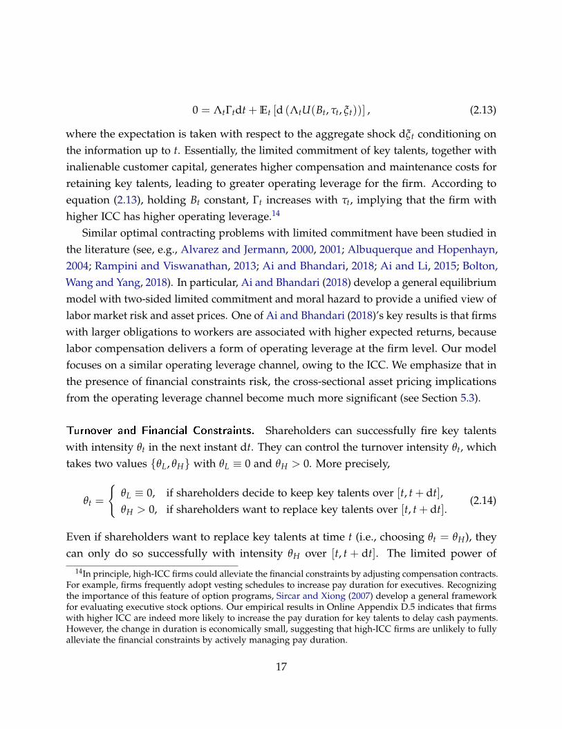
0 = ΛtΓtdt + Et [d (ΛtU(Bt, τt, ξt))] , (2.13)

where the expectation is taken with respect to the aggregate shock dξt conditioning onthe information up to t. Essentially, the limited commitment of key talents, together withinalienable customer capital, generates higher compensation and maintenance costs forretaining key talents, leading to greater operating leverage for the firm. According toequation (2.13), holding Bt constant, Γt increases with τt, implying that the firm withhigher ICC has higher operating leverage.14

Similar optimal contracting problems with limited commitment have been studied inthe literature (see, e.g., Alvarez and Jermann, 2000, 2001; Albuquerque and Hopenhayn,2004; Rampini and Viswanathan, 2013; Ai and Bhandari, 2018; Ai and Li, 2015; Bolton,Wang and Yang, 2018). In particular, Ai and Bhandari (2018) develop a general equilibriummodel with two-sided limited commitment and moral hazard to provide a unified view oflabor market risk and asset prices. One of Ai and Bhandari (2018)’s key results is that firmswith larger obligations to workers are associated with higher expected returns, becauselabor compensation delivers a form of operating leverage at the firm level. Our modelfocuses on a similar operating leverage channel, owing to the ICC. We emphasize that inthe presence of financial constraints risk, the cross-sectional asset pricing implicationsfrom the operating leverage channel become much more significant (see Section 5.3).

Turnover and Financial Constraints. Shareholders can successfully fire key talentswith intensity θt in the next instant dt. They can control the turnover intensity θt, whichtakes two values {θL, θH} with θL ≡ 0 and θH > 0. More precisely,

θt =

{θL ≡ 0, if shareholders decide to keep key talents over [t, t + dt],θH > 0, if shareholders want to replace key talents over [t, t + dt].

(2.14)

Even if shareholders want to replace key talents at time t (i.e., choosing θt = θH), theycan only do so successfully with intensity θH over [t, t + dt]. The limited power of

14In principle, high-ICC firms could alleviate the financial constraints by adjusting compensation contracts.For example, firms frequently adopt vesting schedules to increase pay duration for executives. Recognizingthe importance of this feature of option programs, Sircar and Xiong (2007) develop a general frameworkfor evaluating executive stock options. Our empirical results in Online Appendix D.5 indicates that firmswith higher ICC are indeed more likely to increase the pay duration for key talents to delay cash payments.However, the change in duration is economically small, suggesting that high-ICC firms are unlikely to fullyalleviate the financial constraints by actively managing pay duration.

17

shareholders to replace key talents reflects the latter’ entrenchment, which is estimated tobe the major reason for the low turnover rate observed in the data (see Taylor, 2010). Inour model, shareholders’ choice of replacement intensity θt ∈ {θL, θH} crucially dependson the firm’s current marginal value of internal funds. Intuitively, the firm is morelikely to replace key talents when it is financially constrained, because the requiredcompensation becomes very costly when the marginal value of the firm’s internal fundsis high. The mechanism has been documented and tested extensively in the literature(see, e.g., Brown and Matsa, 2016; Babina, 2017; Baghai et al., 2017). Such endogenousseparations due to heightened financial constraints risk play a crucial role in generatingsizable impacts on firm value and the cross-sectional asset pricing patterns across firmswith different ICC.

Key talents can extract additional rents when firms are financially distressed andexternal financing/restructuring is needed. This phenomenon has been extensivelydocumented in the literature (see, e.g., Bradley and Rosenzweig, 1992; Henderson, 2007;Goyal and Wang, 2017). For example, firms frequently offer pay retention and incentivebonuses to persuade key talents to stay with the firm through the restructuring process.To capture the rent extraction from key talents, we assume that key talents extractλU(Bt, τt, ξt) from shareholders when the firm runs out of cash. This is the amount offunds misappropriated by key talents rather than a deadweight loss that shareholdershave to bear. Particularly, such extraction would never happen when firms are financiallyfrictionless (i.e., γ = ϕ = 0).

2.4 Firm Optimality

Given Kt and it, the firm’s operating profit over [t, t + dt] is given by

dOt = [p min (Bt, eaKt)− (r + δK)Kt]dt︸ ︷︷ ︸production profits

− [φ(it)Bt + Γt]dt︸ ︷︷ ︸hiring costs

+ dCt,︸︷︷︸shocks

(2.15)

where min(Bt, eaKt)dt is the amount of goods sold that is capped by customer capital Bt,and p is the price of goods; the cost of renting the physical capital for production is (r +δK)Ktdt; the total cost of hiring key talents and sales representatives is [φ(st)Bt + Γt]dt;and the firm-specific operating cash flow shock is dCt, as described in (2.5).

18

The firm’s cash holdings evolve as follows:

dWt = dOt + (r− ρ)Wtdt + dHt − dDt, (2.16)

where (r− ρ)Wtdt is the interest income net of cash carrying cost ρ, and Ht and Dt arecumulative issuance and cumulative payout up to t.

The firm rents physical capital Kt, hires it sales representatives, decides the turnoverintensity θt, and chooses payout policy dDt and external financing policy dHt to maximizeshareholder value defined as follows:

V(Wt, Bt, τt, ξt) = maxKs,is,θs,dDs,dHs

E

[∫ ∞

t

Λs

Λt(dDs − dHs − dXs)

], (2.17)

where dXt = [γBt + ϕdHt + λU(Bt, τt, ξt)]1dHt>0 is the total financing cost when externalfinancing occurs 1dHt>0 = 1.

A key simplification in our setup is that the firm’s four-state optimization problem canbe reduced to a three-state problem by exploiting homogeneity. We define the functionv(w, τ, ξ) on D = R+ × (0, 1)× {ξL, ξH} such that

V(W, B, τ, ξ) ≡ v(w, τ, ξ)B, with w = W/B. (2.18)

The normalized value function v(w, τ, ξ) can be solved based on a group of two coupledpartial differential equations with free boundaries. Talent turnover and financial decisionscan be sufficiently characterized by decision boundaries, including the optimal externalequity issuance boundary w(τ, ξ) below which the firm pursues external financing(dH > 0), the optimal payout boundary w(τ, ξ) above which the firm chooses to pay outdividends (dD > 0), and the optimal turnover boundary w(τ, ξ) below which the firmchooses to replace existing key talents (θ = θH > 0). Within the internal liquidity-hoardingregion, there exists a conditional external financing region (w(τ, ξ) < w < w(τ, ξ) + f ),in which the firm issues equity conditional on the arrival of lumpy cash flow shocks f .Figure 2 provides an intuitive illustration of the regions and boundaries.

2.5 Discussions on Modeling Ingredients

The baseline model has three state variables: the cash ratio w, the ICC τ, and the levelof financial constraints risk ξ. These three state variables are the bare minimum for

19

Talent Turnover Talent Stay

External

FinancingInternal Liquidity Hoarding Payout

Conditional

External Financing

Figure 2: Decision boundaries and regions

delivering our key theoretical insights due to the following reasons: first, the cash ratiowt, as well as the financial friction, is necessary because our key mechanism relies onliquidity-driven turnover and financial constraints risk; second, the ICC τt, as well asthe dependence of customer capital on key talents, is necessary because it is the keycross-sectional heterogeneity, and its interaction with the financial constraints is the mainfocus of this paper; third, the level of financial constraints risk ξt is necessary because wefocus on the differential levels of exposure to the aggregate shocks in the level of financialconstraints risk.

We would like to emphasize that the interaction between inalienable customer capitaland financial constraints is crucial for generating significant quantitative effects. Missingeither the ICC or financial constraints would invalidate the model in terms of matchingthe data (see Section 5.3).

2.6 Main Predictions

We illustrate the basic mechanism and main predictions of the model by numericallysolving the model with calibrated parameters presented in Table 9. To highlight theimportance of financial constraints risk, we compare the numerical solutions from ourmodel with those from a model without financial frictions (by setting γ = ϕ = 0).

Cash Holdings and Financial Decisions. Panel A of Figure 3 plots the firm’s normalizedenterprise value v(w, τ, ξL) − w, i.e., the value of the firm’s marketable claims minusthe cash ratio, as a function of the cash ratio in the regime of low financial constraintsrisk (i.e., ξ = ξL). The figure shows that the low-ICC firm (τ = 0.1) has a significantly

20

higher enterprise value relative to the high-ICC firm (τ = 0.6) primarily because talent-dependent customer capital is more costly to maintain. The firm’s enterprise valueincreases with the cash ratio, because the financial constraints risk imposes a deadweightloss through costly equity financing and distorts the firm’s decisions. By contrast, in theabsence of financial frictions, both firms have higher and flat enterprise values.

Our model predicts that the low-ICC firm tends to issue less equity (i.e., optimalfinancing amount w∗l < w∗h) and pay out more dividends (i.e., dividend payout boundarywl < wh). As a result, the low-ICC firm’s endogenous steady-state distribution of cashratios is concentrated at lower levels (see panel D). We provide empirical evidence thatthe firms with lower ICC issue more equity, pay out less dividend, and hold more cashon average (see Appendix C.1). The difference in financial policies can be explained bythe difference in the marginal value of internal funds. Panel B shows that the high-ICCfirm has a higher marginal value of internal funds, because it is more exposed to financialconstraints risk due to greater operating leverage. When the firm’s cash ratios are high,the operating leverage does not increase financial constraints risk much, because internalfunds cushion the firm from cash flow shocks. However, when cash ratios are low, thecompensation required to retain key talents significantly increases the financial constraintsrisk that the high-ICC firm faces. In the frictionless benchmark, the marginal value ofinternal funds for both firms is flat and equal to 1.

Panel C compares the hiring decisions of the two firms. The variation in the en-dogenous marginal value of internal funds suggests that both firms hire fewer salesrepresentatives when cash ratios are low. On average, the low-ICC firm tends to hiremore sales representatives. These implications suggest that financial constraints riskalso distorts the firm’s decisions in the product market. When the financial market hasfrictions, the firm cuts its investment in customer capital to obtain short-term liquidity. Inthe frictionless benchmark, the first-best hiring units are higher for both firms.

Asset Pricing Implications. Panels E and F illustrate the asset pricing implications ofour model by plotting the firms’ exposure to financial-constraints-risk shocks, measuredby the betas with respect to ξ, that is, βξ(w, τ) = v(w, τ, ξH)/v(w, τ, ξL)− 1. Panel Eshows that conditioning on the ICC, firms’ exposure to financial-constraints-risk shocksincreases when their cash ratios decrease. As a result, investors demand higher expectedreturns for the firms with lower cash ratios. Importantly, the difference in betas between

21

0 0.1 0.2 0.3 0.4

0

0.5

1

1.5

2

2.5

3

0 0.1 0.2 0.3 0.4

1

1.5

2

2.5

3

0 0.1 0.2 0.3 0.4

0.06

0.08

0.1

0.12

0 0.1 0.2 0.3 0.4

0

0.05

0.1

0.15

0.2

0.25

0.3

0 0.1 0.2 0.3 0.4

-0.8

-0.6

-0.4

-0.2

0

0 0.2 0.4 0.6 0.8 1

-0.8

-0.6

-0.4

-0.2

0

Figure 3: The model’s basic mechanism and asset pricing implications

the high-ICC and the low-ICC firm decreases with cash ratios.15 Similar patterns areobserved in panel F, in which we compare betas of a high-cash firm (w = 0.2) and alow-cash firm (w = 0.1). Conditioning on the cash ratio, firms’ exposure to financial-constraints-risk shocks becomes more negative as their customer capital becomes moretalent dependent. Importantly, the difference in betas and expected excess returns betweenthe high-cash and the low-cash firm increases with the ICC. By contrast, in the frictionlessbenchmark, betas are almost zero, regardless of the cash ratio and the ICC.

Our model highlights that the interaction between the firm’s ICC and cash ratios has

15The quantitatively differential response to financial-constraints-risk shocks between the low and high-ICC firms also incorporates a countervailing force that dampens the relative response of the high-ICC firm,because an increase in financial constraints risk reduces key talents’ compensation as the outside optionof creating a new firm worsens. From shareholders’ perspective, the reduction in compensation providesinsurance against the regime with high financial constraints risk, increasing the firm’s value. This insuranceeffect is especially beneficial for the high-ICC firm, in which more customer capital is maintained by keytalents. Our numerical solutions suggest that this countervailing force is dominated by the main forcethrough greater operating leverage and customer capital damage due to key talent turnover.

22

crucial implications for asset prices. Thus, the firm’s heterogeneous exposure to financial-constraints-risk shocks is simultaneously reflected in two distinctive cross sections: theICC and the extent to which firms are financially constrained. In other words, themodel implies that the financial-constraints-risk shock can be jointly identified by twocross-sectional return spreads.

Turnover Implications. Our model’s asset pricing implications are closely dependenton talent turnover and the resulting customer capital damage. Panel A of Figure 4compares the effective compensation of high- and low-ICC firms, defined as the mone-tary compensation multiplied by the marginal value of internal funds. Relative to thefrictionless benchmark, the effective compensation to key talents of both the low- andhigh-ICC firms’ increases nonlinearly when cash ratios decrease. The increase in effectivecompensation is more dramatic and nonlinear for the high-ICC firm.

0 0.1 0.2 0.3 0.40

0.05

0.1

0.15

0.2

0.1 0.3 0.5 0.7 0.90

0.1

0.2

0.3

0.4

0.5

0.6

0.1 0.3 0.5 0.7 0.90

0.1

0.2

0.3

0.4

0.5

0.6

Figure 4: Model predictions on effective compensation and talent turnover

The high effective costs of retaining key talents imply that the firm tends to replacekey talents when cash ratios are low. As panel B shows, the firms with higher ICC andlower cash ratios are more likely to replace key talents. The turnover boundary w(τ, ξ)

shifts upward when aggregate financial constraints risk increases. The difference inturnover boundaries w(τ, ξH)− w(τ, ξL) increases with τ. Therefore, our model suggeststhat the high-ICC firm tends to be associated with a greater increase in turnover rateswhen financial constraints risk increases. In other words, customer capital owned by thehigh-ICC firm is more fragile to financial constraints risk.

Intuitively, retaining key talents is beneficial to the firm because, on average, customercapital generates positive net cash inflows. However, when the firm is financially con-

23

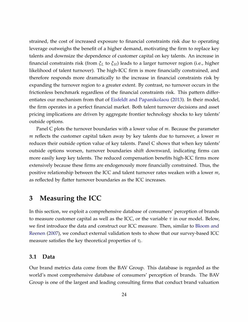
strained, the cost of increased exposure to financial constraints risk due to operatingleverage outweighs the benefit of a higher demand, motivating the firm to replace keytalents and downsize the dependence of customer capital on key talents. An increase infinancial constraints risk (from ξL to ξH) leads to a larger turnover region (i.e., higherlikelihood of talent turnover). The high-ICC firm is more financially constrained, andtherefore responds more dramatically to the increase in financial constraints risk byexpanding the turnover region to a greater extent. By contrast, no turnover occurs in thefrictionless benchmark regardless of the financial constraints risk. This pattern differ-entiates our mechanism from that of Eisfeldt and Papanikolaou (2013). In their model,the firm operates in a perfect financial market. Both talent turnover decisions and assetpricing implications are driven by aggregate frontier technology shocks to key talents’outside options.

Panel C plots the turnover boundaries with a lower value of m. Because the parameterm reflects the customer capital taken away by key talents due to turnover, a lower mreduces their outside option value of key talents. Panel C shows that when key talents’outside options worsen, turnover boundaries shift downward, indicating firms canmore easily keep key talents. The reduced compensation benefits high-ICC firms moreextensively because these firms are endogenously more financially constrained. Thus, thepositive relationship between the ICC and talent turnover rates weaken with a lower m,as reflected by flatter turnover boundaries as the ICC increases.

3 Measuring the ICC

In this section, we exploit a comprehensive database of consumers’ perception of brandsto measure customer capital as well as the ICC, or the variable τ in our model. Below,we first introduce the data and construct our ICC measure. Then, similar to Bloom andReenen (2007), we conduct external validation tests to show that our survey-based ICCmeasure satisfies the key theoretical properties of τt.

3.1 Data

Our brand metrics data come from the BAV Group. This database is regarded as theworld’s most comprehensive database of consumers’ perception of brands. The BAVGroup is one of the largest and leading consulting firms that conduct brand valuation

24

surveys and provide brand development strategies for clients. The BAV brand perceptionsurvey consists of more than 870,000 respondents, and it is constructed to representthe U.S. population according to gender, ethnicity, age, income group, and geographiclocation. The details of the survey have been described by finance and marketing academicpapers (see, e.g., Larkin, 2013; Tavassoli, Sorescu and Chandy, 2014). The BAV surveysare conducted at the brand level. Survey respondents are asked to complete a 45-minutesurvey that yields measures of brand value. The first survey was conducted in 1993, andsince 2001, the surveys have been conducted quarterly. The surveys cover more than 3,000brands and are not biased toward the BAV Group’s clients. The BAV Group updates thelist of brands regularly to include new brands and exclude the ones that have exited themarket, and it does not backfill the survey data. To make the surveys manageable, eachquestionnaire contains fewer than 120 brands that are randomly selected from the list ofbrands.

We identify the firms that own the brands over time, and link the BAV survey datawith Compustat and CRSP. We pay particular attention to the brands involved in mergersand acquisitions to ensure that the brands are assigned correctly to firms. For eachfirm in a given year, we calculate the average scores of various brand metrics over allthe brands owned by the firm.16 Our merged BAV-Compustat-CRSP data span 1993 -2016 and include firms listed on the NYSE, AMEX, and NASDAQ exchanges with sharecodes 10 or 11. We exclude financial firms and utility firms. We have 1,004 unique firmsin total, and on average, about 400 firms in the yearly cross section. The firms in themerged sample collectively own 4,745 unique brands covered by the BAV surveys. Theentry and exit rates of the firms in the merged sample are approximately 7%, whichare comparable to those in the Compustat data. Firms in the merged sample and in theCompustat/CRSP sample have comparable book-to-market ratios and debt-to-asset ratios.The merged sample is biased toward large firms.17 Because the merged sample is not arandom sample of U.S. public firms, in Section 4.1.2 we replicate our asset pricing testsin an extended sample that covers the cross section of all U.S. public firms. We further

16In our sample, 58% of firm-year observations have only one brand. For the firms that own more thanone brand, we use several alternative methods to compute the firm-level brand metrics from the brand-leveldata. We provide details on the construction of firm-level brand metrics in Online Appendix D1. Ourresults are robust to the choice of methods.

17In the merged sample, the median book-to-market ratio, debt-to-asset ratio, market capitalization,and sales are 0.37, 0.55, $4, 915 million, and $5, 115 million, respectively, whereas they are 0.49, 0.44, $420million, and $424 million in the Compustat/CRSP sample. We provide more details on the merged sample,including its distribution across industries, in Online Appendix D2.

25

link the merged BAV-Compustat-CRSP data with Execucomp, BoardEx, and the HarvardBusiness School patent and innovator database (see Li et al., 2014). Online AppendixTable OA.5 presents the summary statistics for the main variables.

3.2 The ICC Measure

Based on the brand perception survey data, the BAV Group has developed two majorbrand metrics to assess the value of firms’ customer capital: brand stature and brandstrength.

Brand Stature. The BAV Group constructs the brand stature measure to capture cus-tomer capital (i.e., brand loyalty of existing and potential customers); see, for example,Gerzema and Lebar (2008). Brand stature is the product of esteem and knowledge. Esteemgauges consumers’ respect and admiration for a brand. The components of esteem are(1) the brand score on “regard” (“How highly do you think of this brand?” on a 7-pointscale) and (2) the fraction of respondents who consider the brand to be of “high quality,”“reliable,” and a “leader.” Esteem reflects brand loyalty, because consumers are proudto be associated with the brand that they hold in high regard. To gauge the credibilityand precision of the esteem measure, BAV designed the knowledge measure to capturethe degree of personal familiarity (“How familiar are you with this brand?” on a 7-pointscale). BAV finds that the past, current, and potential users of a brand tend to ratethemselves as being significantly more knowledgeable. Thus, the knowledge measureserves as an adjustment factor for the esteem measure in quantifying brand stature (i.e.,customer capital defined by brand loyalty of existing and potential customers).

Brand Strength. The BAV Group constructs the brand strength measure to capture theextent to which a brand is perceived to be innovative, distinctive, and managed by adynamic team. Brand strength is the product of energized differentiation and relevance.Energized differentiation is the average fraction of respondents who consider a brandto be “innovative,” “distinctive,” “unique,” “different,” and “dynamic.” “Innovative”captures the innovativeness of the brand. “Distinctive,” “unique,” and “different” capturethe differentiation of a brand from its peers, whereas “dynamic” captures the vibrancy ofthe management team. Energized differentiation is obviously attributed to the uniquecontribution of key talents. The relevance measure (“How relevant do you feel the

26

brand is for you?” on a 7-point scale) serves as an adjustment factor for the energizeddifferentiation measure in quantifying brand strength (i.e., talent-dependent customercapital defined by brand loyalty of existing and potential customers attributed to theunique contribution of key talents). Consumers’ perception of a brand’s energizeddifferentiation can better reflect the firm’s talent-dependent customer capital when theyare more likely to purchase the goods and become the firms’ customers. The relevancemeasure is designed to capture the degree of personal appropriateness for consumers,which largely reflects the possibility for consumers to purchase the goods.

The ICC Measure. The ICC measure should reflect the degree to which customercapital depends on talents; thus, we measure the ICC at the firm level as follows:

The ICC measurei,t ≡brand strengthi,t

brand staturei,t, for firm i in year t. (3.1)

The distribution of our ICC measure is skewed, and we use the log transformation ofthe ICC measure, denoted by ln(ICC). Online Appendix D2 shows that ln(ICC) exhibitsa good amount of variation, with an approximately normal distribution. Moreover,brand stature and brand strength have a similar range and standard deviation. Thus thevariation in ln(ICC) does not predominantly come from either brand stature or brandstrength. To ease the interpretation of regression coefficients in our empirical analyses,we standardize ln(ICC) by its unconditional mean and standard deviation for all firmsacross the entire period. We sort the firms in our sample into five quintiles based on theICC measure. The summary statistics are shown in Table 1.

Because our ICC measure is constructed from consumer surveys of brand loyalty, itdirectly captures the perception of existing and potential customers. The ICC measure isvery different from brand metrics derived from firms’ financial and accounting variables,which have at least two major issues: (1) the estimation error introduced by indirectlyinferring the unobservable characteristics from noisy accounting information, and (2) thepotential measurement bias introduced by using the stale information from accountingnumbers. The BAV survey-based measures are designed to tackle these issues. Inaddition, because the ICC measure is not controlled by firm managers, it is unlikely to bemechanically linked to the outcome financial variables we study.

Let us provide a few concrete examples from the 2010s based on our ICC measure.

27

Table 1: Firm characteristics and the ICC

Median Mean

Portfolios sorted on ICC Low 2 3 4 High Low 2 3 4 High

ln(ICC) (standardized) −1.14 −0.68 −0.27 0.28 1.25 −1.13 −0.66 −0.26 0.23 1.32

Firm characteristicslnsize 8.87 9.13 9.00 8.24 7.63 8.86 9.01 8.92 8.28 7.65lnBEME −0.92 −1.08 −1.03 −0.99 −0.97 −0.98 −1.14 −1.03 −1.00 −1.01lnlev 0.59 0.45 0.14 −0.06 −0.27 0.65 0.52 0.17 −0.07 −0.18Operating profitability (%) 32.57 36.07 31.84 28.55 24.60 39.31 40.57 37.52 29.05 24.59∆Asset/lagged asset (%) 3.58 3.60 3.81 5.68 7.55 7.13 7.07 6.88 11.15 14.49

Cash flow volatilityVol(daily returns) (%) 1.85 1.81 1.92 2.20 2.57 2.21 2.08 2.21 2.51 2.91Vol(sales growth) (%) 7.31 6.41 7.45 8.80 10.01 13.13 10.13 10.94 13.31 17.61Vol(net income/asset) (%) 2.30 2.21 2.64 3.14 3.26 3.37 3.61 4.61 5.77 7.12Vol(EBITDA/asset) (%) 2.02 2.05 2.42 2.66 2.79 2.50 2.79 3.02 3.83 4.33

Key-talent compensationAdministrative expenses/sales (%) 17.35 19.02 22.06 23.67 25.36 18.69 19.67 23.08 25.21 27.58R&D/sales (%) 1.99 1.87 2.31 3.64 10.82 3.86 3.88 4.64 5.99 14.21Executive compensation/sales (%) 0.15 0.20 0.25 0.39 0.50 0.32 0.32 0.42 0.59 0.79

Corporate financial policyCash/lagged asset (%) 6.19 6.71 8.86 12.06 19.42 9.07 9.88 14.32 18.74 25.68∆Cash/net income (%) 3.86 3.60 2.68 6.33 9.08 12.08 8.03 10.63 23.35 24.25∆Equity/lagged asset (%) 0.33 0.48 0.55 0.55 0.64 0.94 1.01 1.23 2.28 3.42Payout/lagged asset (%) 3.39 4.95 5.38 3.35 1.98 5.67 6.96 7.07 5.65 4.89Dividend/lagged asset (%) 1.45 1.91 1.55 0.56 0.00 2.16 2.60 2.30 1.47 1.35Repurchases/lagged asset (%) 1.25 2.22 2.33 1.06 0.18 3.44 4.16 4.54 3.91 3.20

Note: This table presents characteristics of the five portfolios sorted on ICC. We report the mean and median firm characteristics foreach portfolio. Our sample includes the firms listed on the NYSE, AMEX, and NASDAQ exchanges with share codes 10 or 11, overthe period 1993 - 2016. We exclude financial firms and utility firms. The definition of variables is in Online Appendix Table OA.5.

In the automobile industry, Toyota is a typical low-ICC firm that enjoys strong brandrecognition all over the world. Tesla is a typical high-ICC firm whose customer capitalcrucially depends on its R&D team. In the beverage industry, Coca-Cola is a typicallow-ICC firm whose customers’ loyalty relies less on the firm’s current executives orinnovators and more on customers’ own habits and tastes. By contrast, Teavana — aninnovative tea company that sources and shares high-quality teas and “imaginative flavorsfrom around the world” with innovative brewing methods — is a typical high-ICC firm.In the IT and apparel industries, Microsoft and Gap are examples of low-ICC firms, andFacebook and Ralph Lauren are examples of high-ICC firms.

28

3.3 External Validation Tests on the ICC Measure

We conduct external validation tests for our ICC measure. According to our model, if theICC measure captures the ICC (or the variable τt in our model), we expect the following:(1) firms whose talents play relatively more important roles are associated with higherICC; (2) firms with higher ICC τt tends to lose a larger fraction of customer capital upontalent turnover; and (3) firms’ customer capital becomes less talent dependent (i.e., theICC τt decreases) upon talent turnover.

To test the theoretical property (1), we examine the relationship between our ICCmeasure and measures of various intangible assets. Conceptually, customer capital isnot a new type of intangible assets. Instead, it is a synthesis of various intangible assetssuch as innovation and product differentiation, dynamic management, and pure brandrecognition. If our ICC measure is valid to capture the ICC, we expect to see that thefirms whose talents play relatively more important roles are associated with higher valuesof the ICC measure. Therefore, we examine the relation between our ICC measure andR&D expenditures (a measure of innovation and product differentiation), administrativeexpenses/executive compensation (measures of dynamic management), and advertisingexpenditures (a measure of pure brand recognition). Using panel regressions (see Table 2),we find that the firms with higher values of the ICC measure are indeed associated withhigher R&D expenditures, higher administrative expenses, higher executive compensation,and lower advertising expenditures, suggesting that their customer capital depends moreon talents than on pure brand recognition.

We would like to emphasize that customer capital cannot be fully captured by anysingle type of intangible assets because a firm’s investment in one type of intangible assetssuch as R&D may not necessarily increase its customer capital. For example, when a firmincreases its R&D expenditures or administrative expenses, the products and services maynot necessarily improve or they may become less relevant to consumers, and thus theseexpenses will not always lead to higher brand loyalty. In other words, consumers may notappreciate the changes (if any) brought by increased R&D expenditures, administrativeexpenses, or executive compensation. By contrast, our survey-based measure from thedemand side directly reflects consumers’ brand perception, and thus it is able to capturecustomer capital in a more direct manner. Importantly, in Appendix B, we show that theasset pricing implications of our ICC measure cannot be fully explained by any singleintangible-asset measure.

29

Table 2: The ICC measure and measures of intangible assets.

(1) (2) (3) (4) (5)

ln(ICC)t

ln(administrative expenses/sales)t−3:t−1 0.133∗∗∗

[2.970]

ln(R&D/sales)t−3:t−1 0.256∗∗∗

[5.755]

ln(executive compensation/sales)t−3:t−1 0.252∗∗∗

[6.469]

ln(advertising expenditures/asset)t−3:t−1 −0.088∗∗

[−2.478]

ln(OC/asset)t−3:t−1 −0.039

[−1.307]

Firm controls Yes Yes Yes Yes Yes

Industry FEs & Year FEs Yes Yes Yes Yes Yes

Observations 5300 2695 5086 4329 5594

R-squared 0.386 0.468 0.411 0.413 0.382

Note: This table shows the relation between the ICC measure and measures of intangible assets. The dependent variable ln(ICC)is the natural log of the ICC. The independent variables are the natural log of the administrative-expenses-to-sales ratio, the naturallog of the R&D-to-sales ratio, the natural log of the executive-compensation-to-sales ratio, the natural log of the advertisement-to-asset ratio, and the natural log of the organization-capital-to-asset ratio, all computed using the average values from the previousthree years. Our results are robust if we use the average values in other time periods (one year to six years). Administrativeexpenses are estimated as SG&A net of advertising costs, R&D expenses, commissions, and foreign currency adjustments. Executivecompensation is measured by the total compensation for the top five executives of a firm in the Execucomp data. We constructorganization capital (OC), from SG&A expenditures using the perpetual inventory method with missing values being replaced by0. In column (2), we exclude firms with missing R&D, because these firms do not necessarily lack innovation activities (see, e.g.,Koh and Reeb, 2015), unlike zero R&D firms. In column (4), we exclude firms with missing advertising expenditures followingGrullon, Kanatas and Weston (2004) and Belo, Lin and Vitorino (2014). Our results remain robust if we replace missing values inR&D and advertising expenditures by zero. Firm controls include the natural log of market capitalization and the natural log of thebook-to-market ratio. The sample period spans 1993 - 2016. We include t-statistics in brackets. Standard errors are clustered by firmand year. *, **, and *** indicate statistical significance at the 10%, 5%, and 1% levels, respectively.

We also examine the relation between the ICC and organization capital (see Eisfeldtand Papanikolaou, 2013). We find a weak association between these two measures (see col-umn 5), probably because organization capital is constructed from SG&A, which containsboth advertising expenditures and administrative expenses. Advertising expendituresboost pure brand recognition and is negatively related to our ICC measure (see column4 of Table 2), whereas administrative expenses mainly reflect the contribution of talentsand thus are positively related to our ICC measure (see column 1 of Table 2). The weakcorrelation between our ICC measure and organization capital suggests that the twomeasures capture different firm characteristics.

To test the theoretical properties (2) and (3) of our ICC measure, we examine thegrowth rate of brand stature, a measure of customer capital, following the non-retirementturnover of CEOs. As shown in columns (1) and (2) of Table 3, the customer capital

30

Table 3: The ICC measure and changes in customer capital following talent turnover.

(1) (2) (3) (4) (5) (6) (7) (8)

Stature_grt:t+2 Sales_grt:t+2 Asset_grt:t+2 ∆ICCt:t+2

ln(ICC)t−1 × Turnovert −0.041∗ −0.047∗∗ −0.036∗∗ −0.027∗ −0.065∗∗ −0.059∗∗

[−1.804] [−1.982] [−2.402] [−1.794] [−2.320] [−2.302]

Turnovert −0.014 −0.023 −0.073∗∗∗ −0.055∗∗∗ −0.109∗∗∗ −0.095∗∗∗ −0.181∗∗∗ −0.159∗∗

[−0.634] [−1.007] [−3.652] [−3.300] [−4.508] [−3.684] [−2.701] [−2.398]

ln(ICC)t−1 0.141∗∗∗ 0.152∗∗∗ 0.069∗∗∗ 0.033∗∗∗ 0.073∗∗∗ 0.032∗

[17.600] [17.024] [5.919] [3.008] [3.886] [1.745]

Firm controls No Yes No Yes No Yes No Yes

Industry FEs & Year FEs Yes Yes Yes Yes Yes Yes Yes Yes

Observations 3709 3525 4523 4285 4523 4285 4059 3855

R-squared 0.440 0.443 0.170 0.233 0.135 0.211 0.099 0.108

Note: This table shows the relation between the ICC measure and changes in customer capital following talent turnover. The depen-dent variables are the two-year growth rate of brand stature (Stature_grt:t+2), the two-year growth rate of sales (Sales_grt:t+2), thetwo-year growth rate of assets (Asset_grt:t+2), and the two-year change in the ICC (∆ICCt:t+2). CEO turnovert is an indicator variablethat equals 1 if a CEO leaves the firm at age 59 or younger. The main independent variables are lagged standardized ln(ICC)t−1,the turnover indicator, and the interaction term between the two. Firm controls include the natural log of firm market capitalization,the natural log of the book-to-market ratio, the natural log of the debt-to-equity ratio, and the natural log of organization capitalnormalized by assets. We control for year fixed effects and SIC industry fixed effects. The sample spans 1993 - 2016. We includet-statistics in brackets. *, **, and *** indicate statistical significance at the 10%, 5%, and 1% levels, respectively.

of high-ICC firms is more negatively affected by CEO turnover than that of low-ICCfirms. In addition, the sales growth and asset growth of high-ICC firms also react morenegatively to CEO turnover (see columns 3 – 6 of Table 3). Finally, we examine thechanges in ICC after CEO turnover. As shown in columns (7) and (8), the ICC decreasesfollowing CEO turnover, suggesting that firms’ customer capital depends less on talentsafter they leave.

4 Empirical Results

We now test the joint cross-sectional implications of the ICC on stock returns and talentturnover.

4.1 Asset Pricing Tests

We first examine the asset pricing implications of the ICC. We show that firms with higherICC have higher average and risk-adjusted returns. Moreover, we find that the long-shortportfolio sorted on ICC comoves with the financial-constraints-risk factor.

31

4.1.1 Portfolios Sorted on ICC

In this subsection, we document the returns of the stock portfolios sorted on ICC. InJune of year t, we sort firms into five quintiles based on their ICC in year t− 1. Once theportfolios are formed, their monthly returns are tracked from July of year t to June ofyear t + 1. Table 4 shows that the equal-weighted (value-weighted) low-ICC portfolio (Q1)has annualized average excess returns of 10.20% (4.94%). By contrast, the equal-weighted(value-weighted) high-ICC portfolio (Q5) has annualized average excess returns of 16.18%(11.62%). The equal-weighted (value-weighted) portfolio that longs Q5 and shorts Q1 hasa positive and statistically significant annualized return of 5.98% (6.68%). The magnitudeof this return spread (i.e., the ICC spread) is also economically significant because it isclose to the level of equity premium and value premium. The equal-weighted portfoliosare preferred in our analysis, because the cross section includes about 400 firms and theoverweighting of large firms and the resulting diversification failure could be a concernfor the value-weighted portfolios (see, e.g., Gabaix, 2011).

Table 4: Excess returns and alphas of portfolios sorted on ICC

Equal weighted Value weightedPortfolios sorted on ICC 1 (L) 2 3 4 5 (H) 5− 1 1 (L) 2 3 4 5 (H) 5− 1

Average excess returns (%) 10.20∗∗ 12.17∗∗∗12.48∗∗∗13.29∗∗∗16.18∗∗∗ 5.98∗∗ 4.94 9.68∗∗∗ 9.84∗∗∗ 10.04∗∗ 11.62∗∗∗ 6.68∗

[2.53] [3.37] [3.33] [3.14] [3.46] [2.14] [1.56] [3.22] [3.02] [2.43] [2.65] [1.94]

Fama-French three-factor α (%) −0.42 2.94∗ 2.72 2.67 5.50∗∗ 5.92∗∗ −2.53∗ 3.47∗∗∗ 2.89∗ 1.45 4.25∗ 6.77∗∗

(Fama and French, 1993) [−0.23] [1.70] [1.56] [1.32] [2.44] [2.44] [−1.71] [2.70] [1.94] [0.78] [1.92] [2.35]

Carhart four-factor α (%) 1.81 4.84∗∗∗ 4.40∗∗∗ 5.16∗∗∗ 8.00∗∗∗ 6.19∗∗ −2.09 3.11∗∗ 3.08∗∗ 2.43 4.83∗∗ 6.92∗∗

(Carhart, 1997) [1.08] [3.06] [2.68] [2.87] [3.89] [2.51] [−1.41] [2.40] [2.04] [1.32] [2.17] [2.37]

Note: This table shows the equal-weighted and value-weighted average excess returns and alphas for portfolios sorted on ICC. Thesample period spans 1993 - 2016. We include t-statistics in brackets. Standard errors are computed using the Newey-West estimatorallowing for one lag of serial correlation in returns. We annualize the average excess returns and alphas by multiplying them by 12.*, **, and *** indicate statistical significance at the 10%, 5%, and 1% levels, respectively.

Because high- and low-ICC firms may have differential exposure to the priced riskfactors, we also estimate the alphas using the Fama-French three-factor model (see Famaand French, 1993) and the Carhart four-factor model (see Carhart, 1997). We find that thelong-short portfolio sorted on ICC has positive and statistically significant alphas in bothmodels.18

18In Online Appendix Table OA.6, we show that the ICC also has positive and statistically significantalphas in the q-factor model (see Hou, Xue and Zhang, 2015), the Fama-French five-factor model (seeFama and French, 2015), and the Pástor-Stambaugh five-factor model, the latter of which contains theFama-French three factors, the momentum factor, and the Pástor-Stambaugh liquidity factor (see Pástor

32

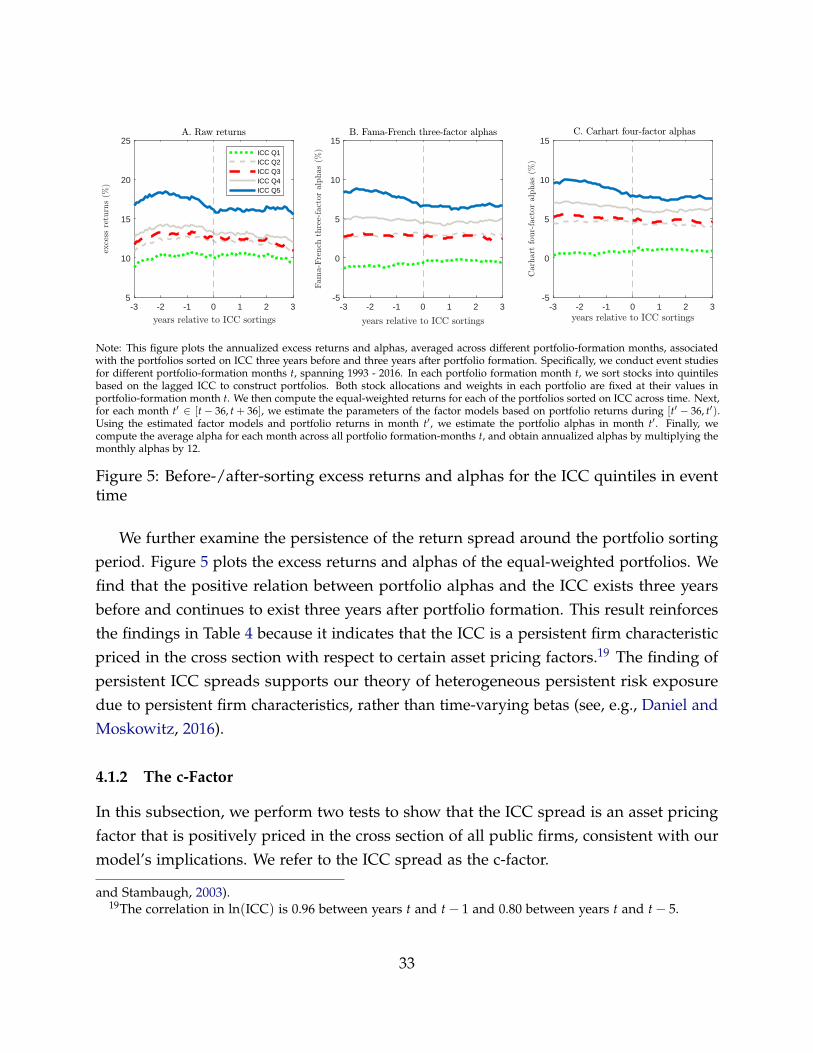
-3 -2 -1 0 1 2 35

10

15

20

25ICC Q1ICC Q2ICC Q3ICC Q4ICC Q5

-3 -2 -1 0 1 2 3-5

0

5

10

15

-3 -2 -1 0 1 2 3-5

0

5

10

15

Note: This figure plots the annualized excess returns and alphas, averaged across different portfolio-formation months, associatedwith the portfolios sorted on ICC three years before and three years after portfolio formation. Specifically, we conduct event studiesfor different portfolio-formation months t, spanning 1993 - 2016. In each portfolio formation month t, we sort stocks into quintilesbased on the lagged ICC to construct portfolios. Both stock allocations and weights in each portfolio are fixed at their values inportfolio-formation month t. We then compute the equal-weighted returns for each of the portfolios sorted on ICC across time. Next,for each month t′ ∈ [t− 36, t + 36], we estimate the parameters of the factor models based on portfolio returns during [t′ − 36, t′).Using the estimated factor models and portfolio returns in month t′, we estimate the portfolio alphas in month t′. Finally, wecompute the average alpha for each month across all portfolio formation-months t, and obtain annualized alphas by multiplying themonthly alphas by 12.

Figure 5: Before-/after-sorting excess returns and alphas for the ICC quintiles in eventtime

We further examine the persistence of the return spread around the portfolio sortingperiod. Figure 5 plots the excess returns and alphas of the equal-weighted portfolios. Wefind that the positive relation between portfolio alphas and the ICC exists three yearsbefore and continues to exist three years after portfolio formation. This result reinforcesthe findings in Table 4 because it indicates that the ICC is a persistent firm characteristicpriced in the cross section with respect to certain asset pricing factors.19 The finding ofpersistent ICC spreads supports our theory of heterogeneous persistent risk exposuredue to persistent firm characteristics, rather than time-varying betas (see, e.g., Daniel andMoskowitz, 2016).

4.1.2 The c-Factor

In this subsection, we perform two tests to show that the ICC spread is an asset pricingfactor that is positively priced in the cross section of all public firms, consistent with ourmodel’s implications. We refer to the ICC spread as the c-factor.

and Stambaugh, 2003).19The correlation in ln(ICC) is 0.96 between years t and t− 1 and 0.80 between years t and t− 5.

33

We first estimate the market price of risk for the ICC spread. As shown in Figure 5,the ICC is persistent and priced in the cross section; thus, an informative portfolio foridentification purposes is the one sorted on the ICC, the corresponding firm characteristic.Estimation based on arbitrary portfolios could be noisy because they may have clusteredbetas (i.e., betas are not dispersed enough in the cross section). We thus sort all U.S.public firms based on their betas with respect to the ICC spread, denoted by βc-factor,which is estimated with a rolling window.20 We then sort firms into quintiles based onβc-factor and compute the average excess returns and alphas of each quintile. We find thatthe firms with higher βc-factor have significantly higher average excess returns and alphas(see Table A.1 in Appendix A), suggesting that the ICC spread is positively priced in thecross section of all U.S. public firms.

To show robustness, we perform further cross-sectional asset pricing tests by includinga broad set of test assets (Fama-French size and value 5 × 5 portfolios, momentumportfolios, industry portfolios, portfolios of treasury bonds, and portfolios of corporatebonds), in addition to the portfolios sorted on ICC. Online Appendix Table OA.10shows that the ICC spread remains positively priced. Moreover, the pricing errors aresignificantly reduced by including the ICC spread in the Fama-French five-factor model.

4.1.3 What Economic Force Does the c-Factor Capture?

Our model implies that firms with higher ICC have greater exposure to financial con-straints risk and therefore must compensate investors with higher expected returns. Inthis subsection, we provide empirical evidence to support the linkage between the ICCand exposure to financial constraints risk.

Specifically, we examine the relation between our c-factor and the return spread oftwo financial constraints measures: (1) the WW index (see Whited and Wu, 2006), whichis structurally estimated to capture the marginal value of internal funds;21 and (2) the BW

20Because the ICC spread is exposed to the risk of traditional asset pricing factors, we control for thesefactors when estimating βc-factor. Pástor and Stambaugh (2003) use the same approach to study the assetpricing implications of their market liquidity factor. They estimate the market liquidity beta in regressionsthat control for the Fama-French three factors. We use the equal-weighted ICC spread to estimate βc-factor,because our sample contains a relatively small number of firms, and thus the value-weighted ICC spreadsuffers from small-sample biases.

21Similar financial-constraints-risk factors are structurally estimated by Eisfeldt and Muir (2016) andBelo, Lin and Yang (2018) using different approaches. We use the WW factor because it is available atmonthly frequency and our model fits into Whited and Wu (2006)’s estimation setup. Several other financialconstraints measures are constructed using the reduced-form approach (see, e.g., Kaplan and Zingales,

34

index, constructed by Buehlmaier and Whited (2018) based on Factiva textual analysis toprovide a direct measure of financial constraints.22 Figure 6 displays the time series andscatter plots of the c-factor, the WW factor, and the BW factor.23 The c-factor is highlycorrelated with both the WW factor and the BW factor, with quarterly correlation being0.59 and 0.68, respectively.

The high correlation between our theoretically motivated c-factor and the two financialconstraints factors has two implications. First, these findings provide empirical supportfor our theory because they suggest that to a large extent, the c-factor also captures thesame financial constraints risk as the WW factor and the BW factor. Second, by connectingour theoretically motivated c-factor to the financial constraints factors, we provide neweconomic insight on why financial constraints could be priced. Specifically, our theorysuggests that one major channel through which the financial-constraints-risk factor affectsstock returns is the ICC.

4.1.4 Financial-Constraints-Risk Shocks versus Primitive Economic Shocks

As discussed in Section 2, financial-constraints-risk shocks could be driven by manyprimitive economic shocks.

Separately identifying pure financial-constraints-risk shocks is challenging, primarilybecause the marginal value of the entire corporate sector’s internal funds cannot increaseor decrease without primitive economic forces. Therefore, similar to Whited and Wu (2006)and Buehlmaier and Whited (2018), we do not intend to disentangle the fundamental

1997; Hadlock and Pierce, 2010), but these estimates do not directly reflect the marginal value of internalfunds.

22Buehlmaier and Whited (2018) develop three financial constraints measures based on textual analysis.The BW index is constructed using the Dow Jones Factiva database as the training sample and it capturesgeneral financial constraints. The other two measures capture financial constraints owing to frictions inissuing equity or issuing debt. We use the BW index because the marginal value of internal funds can beaffected by both types of frictions and thus it is more accurately captured by a measure that also capturesgeneral financial constraints.

23We obtained the BW factor from Buehlmaier and Whited (2018) for the period 1995 - 2010. Thisfactor is calculated as the value-weighted long-short portfolio returns sorted on BW index. We constructthe WW factor following Whited and Wu (2006). First, we sort firms independently based on size andthe WW index into the top 40%, the middle 20%, and the bottom 40%. We then classify firms into thefollowing nine portfolios and calculate the value-weighted return of each portfolio: small size/low WWindex (SL), small size/middle WW index (SM), small size/high WW index (SH), medium size/low WWindex (ML), medium size/middle WW index (MM), medium size/high WW index (MH), large size/lowWW index (BL), large size/middle WW index (BM), and large size/high WW index (BH). The WW factoris constructed as the difference in the returns between the high-constrained firms and the low-constrainedfirms: (BH+MH+SH)/3 - (BL+ML+SL)/3.

35

year

1995 2000 2005 2010 2015

quarterlyreturns(%

)

-40

-20

0

20

40A. Time series of the c-factor and the WW factor

c-factorWW factor

c-factor (%)-30 -20 -10 0 10 20 30

WW

factor

(%)

-50

-25

0

25

50B. Scatter plot

year1995 2000 2005 2010 2015

quarterlyreturns(%

)

-30

-20

-10

0

10

20

30C. Time series of the c-factor and the BW factor

c-factorBW factor

c-factor (%)-30 -20 -10 0 10 20 30

BW

factor

(%)

-15

-10

-5

0

5

10

15D. Scatter plot

Correlation = 0.68

Correlation = 0.59

Note: Panels A and B illustrate the relation between the c-factor and the WW factor. Panels C and D illustrate the relation betweenthe c-factor and the BW factor.

Figure 6: Correlation between the c-factor and the financial constraints factors

drivers of the financial-constraints-risk shock, or to claim that the financial-constraints-riskshock is a new form of primitive economic shocks. In Online Appendix Table OA.11,we show that various primitive shocks, such as uncertainty shocks, TFP shocks, andfinancial-sector shocks are indeed correlated with our c-factor in a coherent way, and theycan explain part of the ICC spread. We find that the ICC spread remains significant aftercontrolling for each primitive economic shock. The ICC spread may well vanish if weexhaustively control for all possible primitive economic shocks. However, identifying allshocks that explain away the ICC spread is not the main objective of our paper.

36

4.1.5 The c-Factor is a Common Factor for Two Cross Sections

Our model implies that the exposure to financial constraints risk is reflected in boththe cross-sectional variation in the ICC and the extent to which firms are financiallyconstrained (panels E and F of Figure 3). Thus, in principle, the c-factor should be able tosimultaneously explain the return spread of the long-short portfolio sorted on ICC andthe degree to which firms are financially constrained. We now provide empirical support.

First, we show that the c-factor is able to explain the ICC spread. Adopting the samemethodology used in Eisfeldt and Papanikolaou (2013, Table VI), we examine the changesin the ICC spread after controlling for the returns of the long-short portfolio sorted onβc-factor. As panels A and B of Table 5 show, the ICC spread decreases significantly andbecomes statistically insignificant.

We continue to examine the return spreads of the BW index in panel C of Table5. Consistent with Buehlmaier and Whited (2018), we find that the alphas for thelong-short portfolio sorted on BW index are positive and statistically significant for thePástor-Stambaugh five-factor model, the Hou-Xue-Zhang q-factor model, and the Fama-French five-factor model. However, the average excess returns and the alphas decreasesignificantly and become statistically insignificant after controlling for the c-factor.

These results from testing the model-implied cross-equation restrictions further cor-roborate our argument that both the ICC and financial constraints measures capture firms’exposure to financial-constraints-risk shocks. However, we would like to emphasize thatfinancial constraints measures and our ICC measure capture different economic concepts.The ICC measure is not an alternative empirical measure for financial constraints. As weshow in Section 2.6, the ICC and the marginal value of internal funds are endogenouslylinked. However, the marginal value of internal funds is not solely determined by theICC; it is also largely determined by other factors such as cash holdings. Conditionalon the same marginal value of internal funds, the exposure to financial-constraints-riskshocks still varies with a firm’s ICC. Thus, even a perfect empirical measure for themarginal value of internal funds should not be considered a “sufficient statistic” for afirm’s exposure to financial-constraints-risk shocks. The primary goal of our paper is toshow that a firm’s ICC is informative and has first-order importance as an additionalcomplementary statistic for summarizing a firm’s exposure to financial-constraints-riskshocks.

37

Table 5: A common factor for two cross sections

Panel A: Equal-weighted excess returns and alphas of the ICC spread

Factor models Excess returns FF3F FF4F PS5F q-factor FF5F

Excess returns and α (%) 5.75∗ 5.91∗∗ 6.12∗∗ 5.59∗∗ 9.45∗∗∗ 9.24∗∗∗

[1.95] [2.32] [2.38] [2.17] [3.57] [3.62]

Excess returns and α controlling for the c-factor (%) 3.55 4.18 3.90 3.47 5.56 5.95

[1.00] [1.14] [1.05] [0.95] [1.36] [1.63]

Panel B: Value-weighted excess returns and alphas of the ICC spread

Factor models Excess returns FF3F FF4F PS5F q-factor FF5F

Excess returns and α (%) 6.42∗ 6.83∗∗ 6.95∗∗ 6.67∗∗ 11.52∗∗∗ 11.77∗∗∗

[1.77] [2.29] [2.31] [2.19] [3.79] [4.04]

Excess returns and α controlling for the c-factor (%) 3.57 4.74 4.26 4.07 7.00 8.08∗∗

[1.13] [1.20] [1.28] [1.36] [1.53] [2.01]

Panel C: Excess returns and alphas of the long-short portfolio sorted on BW index

Factor models Excess returns FF3F FF4F PS5F q-factor FF5F

Excess returns and α (%) 1.05 2.33 2.23 3.39∗∗ 5.02∗∗ 4.60∗∗

[0.56] [1.51] [1.49] [2.60] [2.38] [3.78]

Excess returns and α controlling for the c-factor (%) −1.85 −0.37 −0.45 0.71 0.33 0.62

[−1.52] [−0.26] [−0.29] [0.47] [0.21] [0.39]

Note: Panel A (panel B) tabulates the equal-weighted (value-weighted) excess returns and alphas of the ICC spread, with andwithout controlling for the returns of the long-short portfolio sorted on βc-factor under various factor models. βc-factor is the beta withrespect to the c-factor. The sample period is from 1995 to 2016, because we use data for the first two years to compute the laggedyearly βc-factor. The excess returns and alphas for the ICC spread are different from those in Table 4 due to the difference in thesample period. Panel C tabulates the value-weighted excess returns and alphas of the long-short portfolio sorted on BW index, withand without controlling for the c-factor. The sample period is from 1995 to 2010, during which the BW index is available. We includet-statistics in brackets. Standard errors are computed using the Newey-West estimator allowing for one lag of serial correlationin returns. We annualize the average excess returns and the alphas by multiplying them by 12. *, **, and *** indicate statisticalsignificance at the 10%, 5%, and 1% levels, respectively.

4.1.6 Robustness

Our double-sort analyses in Appendix B indicate that the asset pricing implications ofthe ICC are robust and not explained by other firm characteristics. We further checkthe robustness of our results using the Fama-MacBeth regression method (see Fama andMacBeth, 1973). We regress individual stocks’ returns on ln(ICC) and a battery of returnpredictors, such as size, book-to-market ratio, investment (capex-to-asset ratio), ROA,momentum, and short-term return reversal. Online Appendix Table OA.17 reports theaverage coefficients (in percent) from monthly Fama-MacBeth cross-sectional regressions.The coefficient of the ICC measure is positive and statistically significant. Moreover,following Li (2011), we control for various measures of firms’ R&D activities (R&D-to-sales ratio, R&D-to-asset ratio, R&D-to-capex ratio, R&D-to-number-of-employeesratio, and R&D-to-market-equity ratio). Consistent with the literature (see, e.g., Li,

38

2011; Hirshleifer, Hsu and Li, 2013, 2017), we find that the R&D measures have positivecoefficients in the Fama-MacBeth regressions. The coefficient of the ICC measure remainssignificantly positive after controlling for these R&D measures, suggesting that R&D isunlikely to fully explain the positive relation between the ICC and stock returns.

4.2 Turnover

We now test the model’s predictions on turnover. We show that the ICC is positivelyrelated to the turnover rates of executives and innovators. Moreover, the positive relation-ship is more pronounced during the periods of heightened financial constraints risk andfor firms located in states where the enforcement of non-compete agreements is weaker.

Table 6: The ICC and talent turnover

(1) (2) (3) (4) (5) (6)

Executives Innovators

Turnovert × 100 ln(1 + leavers)t ln(1 + new hires)t

ln(ICC)t−1 1.653∗∗∗ 1.546∗∗∗ 0.163∗∗ 0.170∗∗ 0.156∗∗ 0.158∗∗

[3.621] [3.232] [2.198] [2.299] [2.097] [2.113]

Firm controls Yes Yes Yes Yes Yes Yes

Executive controls Yes Yes – – – –

Industry FEs No Yes No Yes No Yes

Year FEs Yes Yes Yes Yes Yes Yes

Observations 24329 24329 1780 1774 1780 1774

R-squared 0.023 0.032 0.381 0.596 0.385 0.601

Note: This table shows the relation between the ICC and the turnover of executives and innovators. In columns (1) and (2), we studyexecutive turnover. Turnovert is an indicator variable that equals 1 for a given executive-year observation if the executive leaves thefirm at age 59 or below, and 0 otherwise. In columns (3) to (6), we study innovator turnover. A mover in a given year is defined as aninnovator who generates at least one patent in one firm and at least one patent in another firm later in the same year. If innovatorsleave their firms in a given year, they are classified as leavers of their former employers in that year. If innovators join new firmsin a given year, they are classified as new hires of their new employers in that year. The dependent variables are the natural logof 1 plus the number of leavers and the natural log of 1 plus the number of new hires. The main independent variable is laggedstandardized ln(ICC). Firm controls include the natural log of firm market capitalization, the natural log of the book-to-marketratio, the natural log of the debt-to-equity ratio, the natural log of organization capital normalized by assets, and the stock returnin the previous year. Executive controls include genders. We control for year fixed effects with and without SIC-2 industry fixedeffects. The executive turnover sample spans 1993 - 2016, whereas the innovator turnover sample spans 1993 - 2010. We includet-statistics in brackets. Standard errors are clustered by firm and year. *, **, and *** indicate statistical significance at the 10%, 5%,and 1% levels, respectively.

4.2.1 The ICC and Talent Turnover

We first study the relation between the ICC and executive turnover. We focus on theexecutives in the Execucomp database, which covers the top five executives of each S&P

39

500 firm in terms of compensation.24 We find that executive turnover rates are significantlyhigher in the firms with higher ICC (see columns 1 and 2 of Table 6). According to thespecification with both year and industry fixed effects, a one standard deviation increasein ln(ICC) is associated with an increase of 1.546 percentage points in the probability ofexecutive turnover each year, which is roughly one-eighth of the average turnover rate inthe data.

Next, we study the relation between the ICC and innovator turnover. We track theemployment history of innovators based on the HBS patent and innovator database,which provides innovators’ names and affiliations from 1975 to 2010. We find that thefirms with higher ICC are associated with significantly higher innovator turnover rates(see columns 3 – 6 of Table 6). According to the specifications with both year and industryfixed effects, a one-standard-deviation increase in ln(ICC) is approximately associatedwith a 17.0% increase in leavers and a 15.8% increase in new hires.

4.2.2 Interaction with Financial Constraints Risk

Our model implies that the positive relation between the ICC and turnover rates isstronger during periods with heightened financial constraints risk. Section 4.1.3 abovesuggests that a low level of c-factor is associated with heightened financial constraintsrisk. In this section, we thus include the interaction term between ln(ICC) and the yearlyc-factor as the main independent variable.

Table 7 shows that the coefficients for the interaction term are significantly negative,suggesting that the positive relation between the ICC and talent turnover rates is indeedmore pronounced during periods of heightened financial constraints risk. This interactioneffect is economically significant. For example, according to the specification with yearfixed effects (column 1), when the c-factor changes from its mean value (5.8%) to avalue that is two standard deviations below the mean (−27.5%), the sensitivity between

24Because Execucomp provides only limited information on the turnover of executives (especially fornon-CEOs), we further merge Execucomp with BoardEx and use the employment history data in BoardExto identify executive turnover. We focus on those instances of executive turnover that are not due toretirements, because (1) retirement is mostly due to age, health status, and lifestyle choices of executives,none of which reflects firms’ active decisions, and (2) non-retirement turnover is more likely to hurtcustomer capital and thus are more relevant to the mechanism proposed in our paper. We follow theliterature (see, e.g., Parrino, 1997; Jenter and Kanaan, 2015) and use age 60 as the cutoff for the retirementage. Our results are robust to other age cutoffs, such as 65. In Online Appendix D4, we replicate theturnover analyses in two different samples: (1) CEOs only and (2) all managers in the BoardEx dataset. Therelation between the ICC and turnover remains robust.

40

Table 7: The ICC and talent turnover: interaction with financial constraints risk

(1) (2) (3) (4) (5) (6)

Executives Innovators

Turnovert × 100 ln(1 + leavers)t ln(1 + new hires)t

ln(ICC)t−1 1.881∗∗∗ 1.758∗∗∗ 0.208∗∗∗ 0.209∗∗∗ 0.195∗∗ 0.194∗∗

[3.749] [3.449] [2.715] [2.703] [2.557] [2.494]

ln(ICC)t−1 × c-factort−1 −3.915∗∗ −4.263∗∗ −0.410∗∗∗ −0.415∗∗ −0.372∗∗∗ −0.379∗

[−2.344] [−2.533] [−3.970] [−2.672] [−3.337] [−2.052]

Firm controls Yes Yes Yes Yes Yes Yes

Executive controls Yes Yes – – – –

Industry FEs No Yes No Yes No Yes

Year FEs Yes Yes Yes Yes Yes Yes

Observations 24107 24107 1688 1682 1688 1682

R-squared 0.024 0.032 0.385 0.603 0.390 0.606

Note: This table shows the relation between talent turnover and the interaction between the ICC and the yearly c-factor. Thedependent variables, firm controls, executive controls, and fixed effects are defined in Table 6. The main independent variables arelagged standardized ln(ICC) and the product of lagged standardized ln(ICC) and lagged c-factor. We omit the term c-factort−1 inthe regressions because it is absorbed by year fixed effects. The executive turnover sample spans 1993 - 2016, whereas the innovatorturnover sample spans 1993 - 2010. We include t-statistics in brackets. Standard errors are clustered by firm and year. *, **, and ***indicate statistical significance at the 10%, 5%, and 1% levels, respectively.

ln(ICC) and executive turnover increases significantly (the coefficient changes from 1.654to 2.958).25

4.2.3 Interaction with Non-compete Enforceability

Our model implies that the positive relation between the ICC and talent turnover isweaker for firms in which key talents have lower outside option values (see panel C ofFigure 4). Thus, we expect to see a weaker relationship for firms located in states withstronger enforceability of non-compete agreements, because strictly enforced non-competeagreements decrease the outside option value of key talents. To test this hypothesis,we exploit the cross-state variation in the enforceability of non-compete agreements byincluding the interaction term between the ICC and the non-compete enforceability indexas the main independent variable.

As Table 8 shows, the coefficients for the interaction term are significantly negative,suggesting that the positive relation between the ICC and talent turnover rates is indeedweaker when non-compete agreements are more strictly enforced. Consider column 4 asan example. Conditional on the weakest enforceability (index value = 0), a one-standard-deviation increase in ln(ICC) is associated with a 31.8% increase in the number of leavers.

25 1.881 + 5.8%× (−3.915) = 1.654, and 1.881 + (−27.5%)× (−3.915) = 2.958.

41

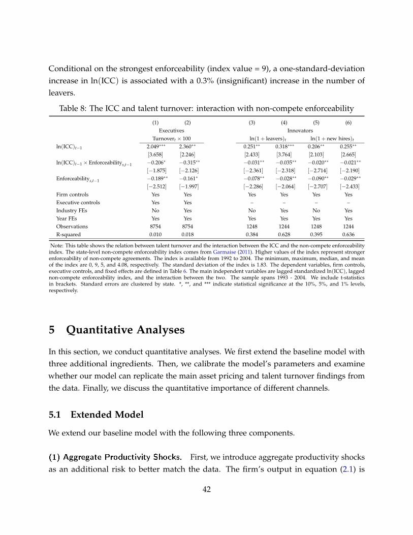
Conditional on the strongest enforceability (index value = 9), a one-standard-deviationincrease in ln(ICC) is associated with a 0.3% (insignificant) increase in the number ofleavers.

Table 8: The ICC and talent turnover: interaction with non-compete enforceability

(1) (2) (3) (4) (5) (6)Executives Innovators

Turnovert × 100 ln(1 + leavers)t ln(1 + new hires)t

ln(ICC)t−1 2.049∗∗∗ 2.360∗∗ 0.251∗∗ 0.318∗∗∗ 0.206∗∗ 0.255∗∗

[3.658] [2.246] [2.433] [3.764] [2.103] [2.665]ln(ICC)t−1 × Enforceabilitys,t−1 −0.206∗ −0.315∗∗ −0.031∗∗ −0.035∗∗ −0.020∗∗ −0.021∗∗

[−1.875] [−2.126] [−2.361] [−2.318] [−2.714] [−2.190]Enforceabilitys,t−1 −0.189∗∗ −0.161∗ −0.078∗∗ −0.028∗∗ −0.090∗∗ −0.029∗∗

[−2.512] [−1.997] [−2.286] [−2.064] [−2.707] [−2.433]Firm controls Yes Yes Yes Yes Yes YesExecutive controls Yes Yes – – – –Industry FEs No Yes No Yes No YesYear FEs Yes Yes Yes Yes Yes YesObservations 8754 8754 1248 1244 1248 1244R-squared 0.010 0.018 0.384 0.628 0.395 0.636

Note: This table shows the relation between talent turnover and the interaction between the ICC and the non-compete enforceabilityindex. The state-level non-compete enforceability index comes from Garmaise (2011). Higher values of the index represent strongerenforceability of non-compete agreements. The index is available from 1992 to 2004. The minimum, maximum, median, and meanof the index are 0, 9, 5, and 4.08, respectively. The standard deviation of the index is 1.83. The dependent variables, firm controls,executive controls, and fixed effects are defined in Table 6. The main independent variables are lagged standardized ln(ICC), laggednon-compete enforceability index, and the interaction between the two. The sample spans 1993 - 2004. We include t-statisticsin brackets. Standard errors are clustered by state. *, **, and *** indicate statistical significance at the 10%, 5%, and 1% levels,respectively.

5 Quantitative Analyses

In this section, we conduct quantitative analyses. We first extend the baseline model withthree additional ingredients. Then, we calibrate the model’s parameters and examinewhether our model can replicate the main asset pricing and talent turnover findings fromthe data. Finally, we discuss the quantitative importance of different channels.

5.1 Extended Model

We extend our baseline model with the following three components.

(1) Aggregate Productivity Shocks. First, we introduce aggregate productivity shocksas an additional risk to better match the data. The firm’s output in equation (2.1) is

42

affected by an aggregate productivity shock at evolving as follows:

dat = −µa(at − a)dt + σa√

atdZa,t, (5.1)

where Za,t is a standard Brownian motion independent of Zc,t. We assume that 2µaa > σ2a

to guarantee at > 0. The pricing kernel (2.6) thus becomes

dΛt

Λt= −rdt− κadZa,t + ∑

ξ ′ 6=ξt

[e−κ(ξt ,ξ′) − 1

](dN(ξt,ξ ′)

t − q(ξt,ξ ′)dt), (5.2)

where κa > 0 is the market price of risk for aggregate productivity shocks.

(2) Exogenous Firm-Speci�c Variations in the ICC. Second, to better match the cross-sectional distribution of talent compensation, we introduce an exogenous firm-specificidiosyncratic shock dZω,t to firms’ ICC. Thus, equation (2.7) is modified as

dωt = −µω(ωt −ω)dt +[ln(1−me−ωt

)− ln (1−m)

]dJt︸ ︷︷ ︸

baseline endogenous turnover

+ σω√

ωtdZω,t.︸ ︷︷ ︸exogenous shock

(5.3)

We assume that 2µωω > σ2ω. The process Zω,t is an idiosyncratic standard Brownian

motion, independent of Za,t and Zc,t. Equation (2.9) is rewritten as

Vnew(Bt, τt, at, ξt) = maxW∗

V(W∗, Bnewt , τ, at, ξt)−W∗ −Φ(W∗; Bnew

t ).

(3) Non-pecuniary Private Bene�ts. Third, we introduce another unique feature ofcustomer capital — the non-pecuniary private benefits, in addition to the inalienability.When managing a firm with customer capital Bt, key talents enjoy non-pecuniary privatebenefits hBt with a positive constant h.26 The promise-keeping constraint equation (2.13)

26The assumption that non-pecuniary private benefits are proportional to customer capital Bt reflects thefindings and discussions in the existing literature. For example, key talents can gain identity-based benefits(see Akerlof and Kranton, 2005) while working at the firms with strong brand value, because the firmswith stronger brands offer key talents more opportunities for self-enhancement, higher visibility amongtheir peers, and a greater likelihood of being seen as successful (see Tavassoli, Sorescu and Chandy, 2014).Moreover, future employers may rely on the brand affiliation as a credible indicator of human capital quality.Thus, working for high brand value firms benefits key talents by signaling their unobserved abilities (seeWeiss, 1995). The proportional non-pecuniary private benefits for key talents hBt are commonly adopted inthe literature as a parsimonious modeling technique (see, e.g., Eisfeldt and Rampini, 2008).

43

Table 9: Calibration

Parameters Symbol Value Parameters Symbol Value

Risk-free rate r 5% Damage ratio of talent-dependent customer capital m 0.35

Fixed financing costs γ 0.01 New customer capital created by a new firm ` 0.2

Variable financing costs ϕ 0.06 Private benefits h 0.011

Long-run average aggregate productivity a 1 Long-run fraction of talent-dependent customer capital ω 0.9

Mean reversion of aggregate productivity µa 0.275 Mean reversion of talent-dependent customer capital µω 0.038

Volatility of aggregate productivity σa 0.07 Volatility of talent-dependent customer capital σω 0.19

Physical capital depreciation rate δK 0.1 Customer capital depreciation rate δB 0.15

Cash-carrying costs ρ 1.5% Replacement intensity θH 0.19

Price of goods p 0.46 Idiosyncratic shocks to cash flows σc 0.15

Rent extraction λ 0.06 Lumpy cash flow shock size f 0.1

Effective matching efficiency ψ 0.75 Lumpy cash flow shock frequency ξL, ξH 0, 0.5

Sales’ representative hiring costs (scale) α 5.0 Price of risk of productivity shocks κa 0.4

Sales’ representative hiring costs (convex) η 2 Price of risk of financial-constraints-risk shocks κ(ξL ,ξH ) − ln(3)

Transition intensities q(ξH ,ξL) 0.2 κ(ξH ,ξL) ln(3)

q(ξL ,ξH ) 0.16

is rewritten as0 = Λt(Γt + hBt)dt + Et [d (ΛtU(Bt, τt, at, ξt))] . (5.4)

With the introduction of private benefits, all else equal, we can see that Γt decreaseswith Bt, suggesting that the firm with a weaker brand (smaller Bt) needs to offer a greatercompensating wage differential to keep key talents, due to smaller non-pecuniary privatebenefits. We provide supporting evidence in Appendix C.2.

5.2 Calibration and Parameter Choices

We discipline parameters based on both existing estimates and micro data (see Table 9).

Externally Determined Parameters. The annual interest rate is r = 5%. The deprecia-tion rate of physical capital is δK = 10% per year. We choose the variable financing costϕ = 6% based on the estimates of Altinkilic and Hansen (2000). Following Bolton, Chenand Wang (2011, 2013), we set the fixed financing cost γ = 1% and the cash-carryingcost ρ = 1.5%. We set the effective matching efficiency ψ = 0.75.27 We consider a

27In Online Appendix A1, we show that ψ = ψnχ−1 in a model with micro-founded customer capitalaccumulation based on competitive search. The effective matching efficiency ψ is calibrated as follows.We normalize the matching efficiency ψ and the disutility of search to 1. We set χ = 1.12, which impliesthat the elasticity parameter in the Cobb-Douglas matching function is χ−1

χ = 0.11, consistent with Gourioand Rudanko (2014)’s estimate based on the share of the labor force in sales-related occupations and the

44

quadratic cost function of hiring sales representatives; that is, η = 2. We set δB = 15%within the typical 10%− 25% range of the annual customer turnover rate (see Gourio andRudanko, 2014). We set m = 0.35, so that in our model, key talents leave with 35% oftalent-dependent customer capital.28

The long-run average aggregate productivity a is normalized to 1. We set µa = 0.275,following Gomes, Kogan and Zhang (2003). The transition intensities, q(ξL,ξH) = 0.16 andq(ξH ,ξL) = 0.20, are estimated using the regime-switching dynamics of the ICC spread. Theestimates are consistent with the average length of business cycles, which is 10 years. Weset the price of risk of productivity shocks to κa = 0.4 similar to Eisfeldt and Papanikolaou(2013), and the price of risk of financial-constraints-risk shocks to κ(ξL,ξH) = − ln(3) andκ(ξH ,ξL) = ln(3), similar to Bolton, Chen and Wang (2013). The risk-neutral transitionintensities are q(ξ,ξ ′) = e−κ(ξ,ξ ′)q(ξ,ξ ′) between two different levels of financial constraintsrisk ξ 6= ξ ′.

Internally Calibrated Parameters. The remaining parameters are calibrated by match-ing relevant moments. We simulate a sample of 1,000 firms for 100 years according tothe computed policy functions. The first 20 years are dropped as burn-in. When keytalents leave the firm, new firms are created and included in the sample for the remainingsimulation period. We then compute the model-implied moments and adjust parametersuntil these moments are in line with their values in the data (see Table 10).

We set the price of goods p = 0.46 to match the average cash-asset ratio. We set rentextraction rate λ = 0.06 so that the retention bonuses are between 30% and 70% of keytalents’ compensation (see Goyal and Wang, 2017). We calibrate the hiring cost coefficientα = 5.0 to target the average advertising expenditures as a percent of sales. We set ` = 0.2to match the average key talents’ compensation as a percentage of sales. We set the talentreplacement intensity θH = 19% to match the average executive turnover rate.

Because our empirical ICC measure does not have the same units as τt in our model, we

amount of time consumers spend shopping. Finally, we set the maximum discount n to 0.10 to ensure thatthe firm makes profits from new customers even if the highest initial discounts are offered.

28In the existing literature, several papers have developed models with this feature. For example, Lustig,Syverson and Nieuwerburgh (2011) match the increase in intra-industry wage inequality by assumingthat 50% of organization capital is transferred when the manager switches to a new firm. Eisfeldt andPapanikolaou (2013)’s model assumes that key talents can leave with all intangible capital. Bolton, Wangand Yang (2018)’s benchmark calibration assumes that the entrepreneur would be 20% less efficient if he orshe walks away from the firm.

45

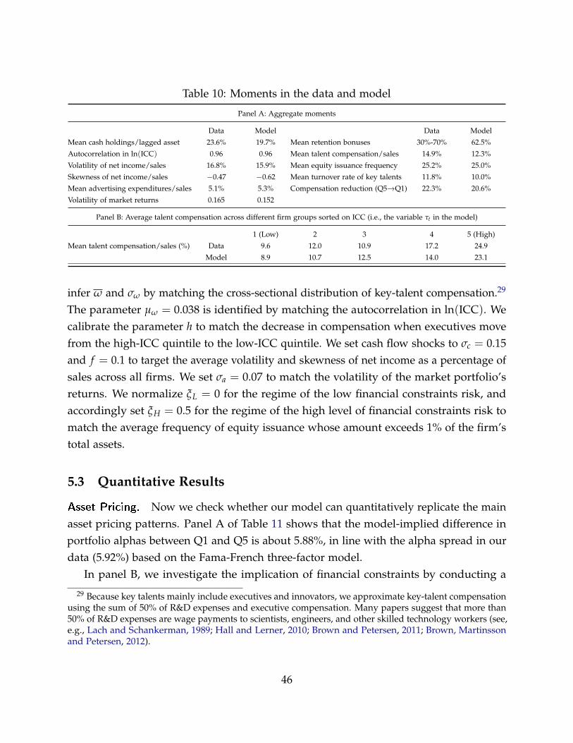
Table 10: Moments in the data and model

Panel A: Aggregate moments

Data Model Data Model

Mean cash holdings/lagged asset 23.6% 19.7% Mean retention bonuses 30%-70% 62.5%

Autocorrelation in ln(ICC) 0.96 0.96 Mean talent compensation/sales 14.9% 12.3%

Volatility of net income/sales 16.8% 15.9% Mean equity issuance frequency 25.2% 25.0%

Skewness of net income/sales −0.47 −0.62 Mean turnover rate of key talents 11.8% 10.0%

Mean advertising expenditures/sales 5.1% 5.3% Compensation reduction (Q5→Q1) 22.3% 20.6%

Volatility of market returns 0.165 0.152

Panel B: Average talent compensation across different firm groups sorted on ICC (i.e., the variable τt in the model)

1 (Low) 2 3 4 5 (High)

Mean talent compensation/sales (%) Data 9.6 12.0 10.9 17.2 24.9

Model 8.9 10.7 12.5 14.0 23.1

infer ω and σω by matching the cross-sectional distribution of key-talent compensation.29

The parameter µω = 0.038 is identified by matching the autocorrelation in ln(ICC). Wecalibrate the parameter h to match the decrease in compensation when executives movefrom the high-ICC quintile to the low-ICC quintile. We set cash flow shocks to σc = 0.15and f = 0.1 to target the average volatility and skewness of net income as a percentage ofsales across all firms. We set σa = 0.07 to match the volatility of the market portfolio’sreturns. We normalize ξL = 0 for the regime of the low financial constraints risk, andaccordingly set ξH = 0.5 for the regime of the high level of financial constraints risk tomatch the average frequency of equity issuance whose amount exceeds 1% of the firm’stotal assets.

5.3 Quantitative Results

Asset Pricing. Now we check whether our model can quantitatively replicate the mainasset pricing patterns. Panel A of Table 11 shows that the model-implied difference inportfolio alphas between Q1 and Q5 is about 5.88%, in line with the alpha spread in ourdata (5.92%) based on the Fama-French three-factor model.

In panel B, we investigate the implication of financial constraints by conducting a

29 Because key talents mainly include executives and innovators, we approximate key-talent compensationusing the sum of 50% of R&D expenses and executive compensation. Many papers suggest that more than50% of R&D expenses are wage payments to scientists, engineers, and other skilled technology workers (see,e.g., Lach and Schankerman, 1989; Hall and Lerner, 2010; Brown and Petersen, 2011; Brown, Martinssonand Petersen, 2012).

46

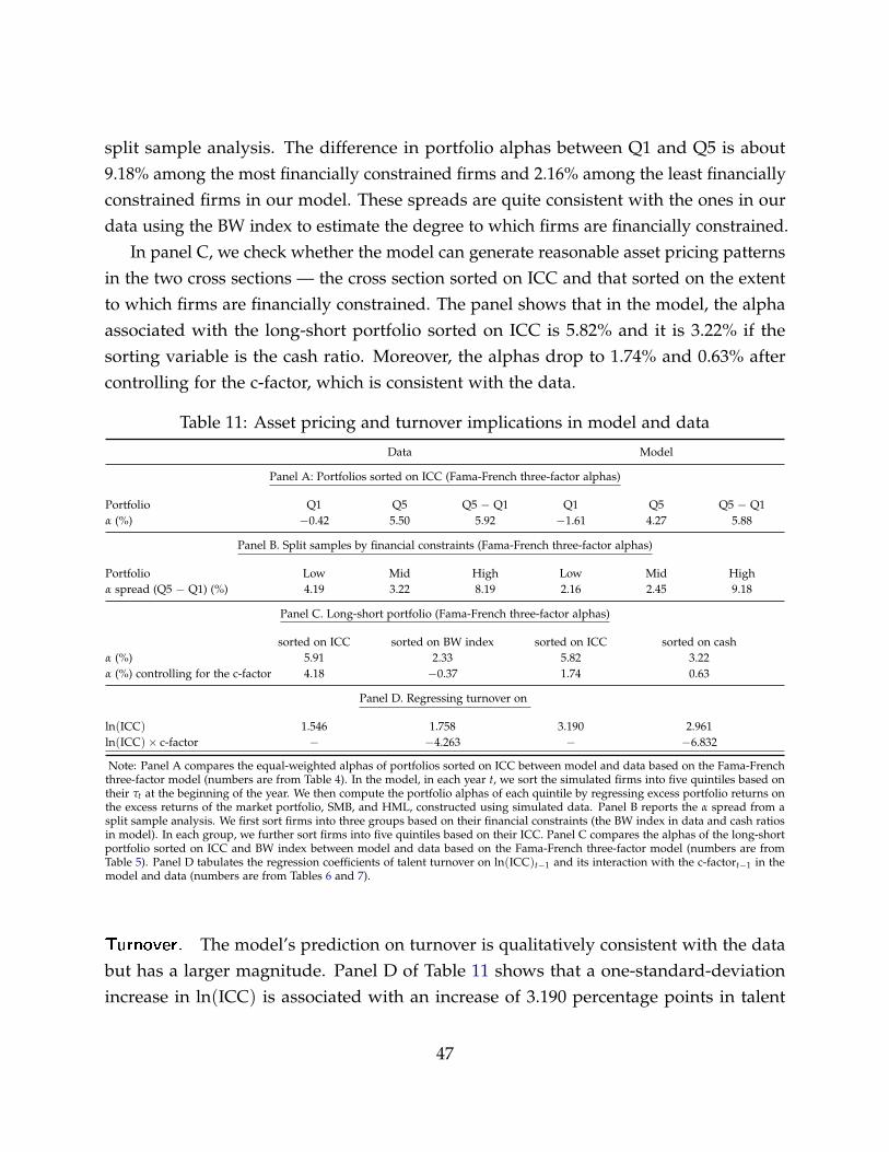
split sample analysis. The difference in portfolio alphas between Q1 and Q5 is about9.18% among the most financially constrained firms and 2.16% among the least financiallyconstrained firms in our model. These spreads are quite consistent with the ones in ourdata using the BW index to estimate the degree to which firms are financially constrained.

In panel C, we check whether the model can generate reasonable asset pricing patternsin the two cross sections — the cross section sorted on ICC and that sorted on the extentto which firms are financially constrained. The panel shows that in the model, the alphaassociated with the long-short portfolio sorted on ICC is 5.82% and it is 3.22% if thesorting variable is the cash ratio. Moreover, the alphas drop to 1.74% and 0.63% aftercontrolling for the c-factor, which is consistent with the data.

Table 11: Asset pricing and turnover implications in model and data

Data Model

Panel A: Portfolios sorted on ICC (Fama-French three-factor alphas)

Portfolio Q1 Q5 Q5 − Q1 Q1 Q5 Q5 − Q1α (%) −0.42 5.50 5.92 −1.61 4.27 5.88

Panel B. Split samples by financial constraints (Fama-French three-factor alphas)

Portfolio Low Mid High Low Mid Highα spread (Q5 − Q1) (%) 4.19 3.22 8.19 2.16 2.45 9.18

Panel C. Long-short portfolio (Fama-French three-factor alphas)

sorted on ICC sorted on BW index sorted on ICC sorted on cashα (%) 5.91 2.33 5.82 3.22α (%) controlling for the c-factor 4.18 −0.37 1.74 0.63

Panel D. Regressing turnover on

ln(ICC) 1.546 1.758 3.190 2.961ln(ICC)× c-factor − −4.263 − −6.832

Note: Panel A compares the equal-weighted alphas of portfolios sorted on ICC between model and data based on the Fama-Frenchthree-factor model (numbers are from Table 4). In the model, in each year t, we sort the simulated firms into five quintiles based ontheir τt at the beginning of the year. We then compute the portfolio alphas of each quintile by regressing excess portfolio returns onthe excess returns of the market portfolio, SMB, and HML, constructed using simulated data. Panel B reports the α spread from asplit sample analysis. We first sort firms into three groups based on their financial constraints (the BW index in data and cash ratiosin model). In each group, we further sort firms into five quintiles based on their ICC. Panel C compares the alphas of the long-shortportfolio sorted on ICC and BW index between model and data based on the Fama-French three-factor model (numbers are fromTable 5). Panel D tabulates the regression coefficients of talent turnover on ln(ICC)t−1 and its interaction with the c-factort−1 in themodel and data (numbers are from Tables 6 and 7).

Turnover. The model’s prediction on turnover is qualitatively consistent with the databut has a larger magnitude. Panel D of Table 11 shows that a one-standard-deviationincrease in ln(ICC) is associated with an increase of 3.190 percentage points in talent

47

Table 12: Inspecting the model mechanisms

α spread on the ICC (%) α spread on cash ratio (%) Annual turnover rate

Full model 5.88 3.25 0.1No ICC (m = 0) 0.27 0.28 0No financing costs (γ = ϕ = 0) 0.59 0 0No private benefits (h = 0) 4.73 3.09 0.12No entrenchment (θH = ∞) 2.72 1.33 0.25

turnover in the model, as compared with an increase of 1.546 percentage points in thedata. Regarding the interaction effect with financial constraints risk, panel D shows thatthe coefficient is −6.832 in the model, and −4.263 in the data.30

Inspecting the Mechanisms in the Model. In Table 12, we conduct the quantitativecomparative static analyses by turning off the key frictions one at a time.

The crucial feature of customer capital is its inalienability associated with key talents.If we instead assume that the turnover of key talents does not damage customer capital(by setting m = 0), the α spread drops to 0.27% and the annual turnover rate also dropsto 0. This is because the value of outside options is very low for key talents, and thusfirms can keep key talents at very low costs. Moreover, as firms become less financiallyconstrained due to the absence of talent compensation, the α spread on the cash ratio alsodrops significantly to 0.28%. If we assume that firms have access to a perfect financialmarket (by setting γ = ϕ = 0), the α spread on the ICC drops significantly to 0.59%.Moreover, both the spread on the cash ratio and the annual turnover rate become zero.These results collectively suggest that the interaction between the ICC and financialconstraints is what jointly determines the quantitative implications of the model in thetwo cross sections.

If we assume no non-pecuniary private benefits are associated with customer capital(by setting h = 0), the α spreads on the ICC and on the cash ratio would drop to 4.73%and 3.09%, respectively. Key talents would ask for higher compensation in the absence ofnon-pecuniary private benefits. The α spreads are lower because non-pecuniary privatebenefits mitigate the operating leverage for low-ICC firms to a larger extent. The annualturnover rate would increase by 2% as firms become more financially constrained due to

30We do not report the model’s quantitative implication on the interaction effect with non-competeenforceability (the results in Table 8), because it is not clear how the variation in the state-level non-competeenforcement index can be quantitatively translated to the variation in the model parameter m. However, aswe show in panel C of Figure 4, our model’s prediction is qualitatively consistent with the data.

48

higher compensation.Finally, we study the role of talents’ entrenchment. If we assume that shareholders can

replace key talents freely (by setting θH = ∞), the implied annual turnover rate wouldincrease to 25%, much larger than what we see in the data. Moreover, because replacingexisting key talents with new talents receiving less compensation essentially mitigatesfirms’ financial constraints, the α spreads on the ICC and the cash ratio would dropsignificantly to 2.72% and 1.33%, respectively.

6 Conclusions

This paper is the first to study the fragility of customer capital due to its inalienabilitycaused by limited legal enforcement, and more importantly, its interaction with financialconstraints such as in Bolton, Chen and Wang (2011). The model shows that the financial-constraints-risk shock (see Whited and Wu, 2006; Buehlmaier and Whited, 2018), asan aggregate economic shock, has strong asset pricing implications and is significantlypriced in the cross section. Particularly, the model shows that firms’ heterogeneousresponse to aggregate financial-constraints-risk shocks, in terms of their stock returnsand talent turnover rates, is simultaneously reflected in two different cross sections — thecross section sorted on ICC and that sorted on the extent to which firms are financiallyconstrained.

Based on a proprietary, granular brand perception survey database, we find empiricalevidence strongly supporting the model’s implications. The firms with higher ICC havehigher average (risk-adjusted) excess returns. The ICC spread is highly correlated withthe financial-constraints-risk factor constructed based on Whited and Wu (2006) andBuehlmaier and Whited (2018). Moreover, the firms with higher ICC are associatedwith higher talent turnover rates, and this pattern is more pronounced in the periods ofheightened financial constraints risk.

ReferencesAaker, David A. 2012. Building Strong Brands. Simon and Schuster.

Ai, Hengjie, and Anmol Bhandari. 2018. “Asset Pricing with Endogenously Uninsurable Tail Risks.” NBERWorking Paper.

49

Ai, Hengjie, and Dana Kiku. 2013. “Growth to Value: Option Exercise and the Cross Section of EquityReturns.” Journal of Financial Economics, 107(2): 325–349.

Ai, Hengjie, and Rui Li. 2015. “Investment and CEO compensation under limited commitment.” Journal ofFinancial Economics, 116(3): 452 – 472.

Ai, Hengjie, Kai Li, Jun Li, and Christian Schlag. 2017. “The Collateralizability Premium.” WorkingPaper.

Ai, Hengjie, Mariano Massimiliano Croce, and Kai Li. 2013. “Toward a Quantitative General EquilibriumAsset Pricing Model with Intangible Capital.” Review of Financial Studies, 26(2): 491–530.

Akerlof, George A., and Rachel E. Kranton. 2005. “Identity and the Economics of Organizations.” Journalof Economic Perspectives, 19(1): 9–32.

Albuquerque, Rui, and Hugo A. Hopenhayn. 2004. “Optimal Lending Contracts and Firm Dynamics.”Review of Economic Studies, 71(2): 285–315.

Altinkilic, Oya, and Robert S. Hansen. 2000. “Are There Economies of Scale in Underwriting Fees?Evidence of Rising External Financing Costs.” Review of Financial Studies, 13(1): 191–218.

Alvarez, Fernando, and Urban J. Jermann. 2000. “Efficiency, Equilibrium, and Asset Pricing with Risk ofDefault.” Econometrica, 68(4): 775–797.

Alvarez, Fernando, and Urban J. Jermann. 2001. “Quantitative Asset Pricing Implications of EndogenousSolvency Constraints.” Review of Financial Studies, 14(4): 1117–1151.

Arrow, Kenneth. 1999. “Observations on Social Capital.” In Social Capital. , ed. Serageldin-I. Dasgupta, P. AMultifaceted Perspective. Washington: The World Bank.

Babina, Tania. 2017. “Destructive Creation at Work: How Financial Distress Spurs Entrepreneurship.”Working Paper.

Baghai, Ramin, Rui Silva, Viktor Thell, and Vikrant Vig. 2017. “Talent in Distressed Firms: Investigatingthe Labor Costs of Financial Distress.” Working Paper.

Banerjee, Shantanu, Sudipto Dasgupta, and Yungsan Kim. 2008. “Buyer-Supplier Relationships and theStakeholder Theory of Capital Structure.” Journal of Finance, 63(5): 2507–2552.

Baron, Matthew, and Wei Xiong. 2017. “Credit Expansion and Neglected Crash Risk.” Quarterly Journal ofEconomics, 132(2): 713–764.

Belo, Frederico, and Xiaoji Lin. 2012. “The Inventory Growth Spread.” Review of Financial Studies, 25(1): 278–313.

Belo, Frederico, Vito Gala, Juliana Salomao, and Maria Ana Vitorino. 2018. “Decomposing Firm Value.”Working Paper.

Belo, Frederico, Xiaoji Lin, and Fan Yang. 2018. “External Equity Financing Shocks, Financial Flows, andAsset Prices.” Review of Financial Studies, forthcoming.

Belo, Frederico, Xiaoji Lin, and Maria Ana Vitorino. 2014. “Brand Capital and Firm Value.” Review ofEconomic Dynamics, 17(1): 150–169.

50

Belo, Frederico, Xiaoji Lin, and Santiago Bazdresch. 2014. “Labor Hiring, Investment, and Stock ReturnPredictability in the Cross Section.” Journal of Political Economy, 122(1): 129–177.

Belo, Frederico, Xiaoji Lin, Jun Li, and Xiaofei Zhao. 2017. “Labor-Force Heterogeneity and Asset Prices:The Importance of Skilled Labor.” Review of Financial Studies, 30(10): 3669–3709.

Berk, Jonathan B., Richard C. Green, and Vasant Naik. 1999. “Optimal Investment, Growth Options, andSecurity Returns.” Journal of Finance, 54(5): 1553–1607.

Berk, Jonathan B., Richard Stanton, and Josef Zechner. 2010. “Human Capital, Bankruptcy, and CapitalStructure.” Journal of Finance, 65(3): 891–926.

Bloom, Nicholas. 2009. “The Impact of Uncertainty Shocks.” Econometrica, 77(3): 623–685.

Bloom, Nicholas, and John Van Reenen. 2007. “Measuring and Explaining Management Practices AcrossFirms and Countries.” Quarterly Journal of Economics, 122(4): 1351–1408.

Bolton, Patrick, Hui Chen, and Neng Wang. 2011. “A Unified Theory of Tobin’s q, Corporate Investment,Financing, and Risk Management.” Journal of Finance, 66(5): 1545–1578.

Bolton, Patrick, Hui Chen, and Neng Wang. 2013. “Market Timing, Investment, and Risk Management.”Journal of Financial Economics, 109(1): 40–62.

Bolton, Patrick, Jose Scheinkman, and Wei Xiong. 2006. “Executive Compensation and Short-TermistBehaviour in Speculative Markets.” Review of Economic Studies, 73(3): 577–610.

Bolton, Patrick, Neng Wang, and Jinqiang Yang. 2018. “Liquidity and Risk Management: CoordinatingInvestment and Compensation Policies.” Journal of Finance, forthcoming.

Bradley, Michael, and Michael Rosenzweig. 1992. “The Untenable Case for Chapter 11.” Yale Law Review,101(5): 1043–1089.

Bronnenberg, Bart J., Jean-Pierre H. Dubé, and Matthew Gentzkow. 2012. “The Evolution of BrandPreferences: Evidence from Consumer Migration.” American Economic Review, 102(6): 2472–2508.

Brown, James R., and Bruce C. Petersen. 2011. “Cash Holdings and R&D Smoothing.” Journal of CorporateFinance, 17(3): 694–709.

Brown, James R., Gustav Martinsson, and Bruce C. Petersen. 2012. “Do Financing Constraints Matter forR&D?” European Economic Review, 56(8): 1512–1529.

Brown, Jennifer, and David A. Matsa. 2016. “Boarding a Sinking Ship? An Investigation of Job Applicationsto Distressed Firms.” Journal of Finance, 71(2): 507–550.

Buehlmaier, Matthias MM, and Toni M Whited. 2018. “Are Financial Constraints Priced? Evidence fromTextual Analysis.” Review of Financial Studies, 31(7): 2693–2728.

Buera, Francisco J., and Yongseok Shin. 2013. “Financial Frictions and the Persistence of History: AQuantitative Exploration.” Journal of Political Economy, 121(2): 221–272.

Cable, Daniel M, and Daniel B. Turban. 2003. “The Value of Organizational Reputation in the RecruitmentContext: A Brand-Equity Perspective.” Journal of Applied Social Psychology, 33(11): 2244–2266.

51

Campbell, John, Jens Hilscher, and Jan Szilagyi. 2008. “In Search of Distress Risk.” Journal of Finance,63(6): 2899–2939.

Carhart, Mark M. 1997. “On Persistence in Mutual Fund Performance.” Journal of Finance, 52(1): 57–82.

Chevalier, Judith A., and David S. Scharfstein. 1996. “Capital-Market Imperfections and CountercyclicalMarkups: Theory and Evidence.” American Economic Review, 86(4): 703–725.

Christiano, Lawrence J., Roberto Motto, and Massimo Rostagno. 2014. “Risk Shocks.” American EconomicReview, 104(1): 27–65.

Cochrane, John H. 1991. “ Production-Based Asset Pricing and the Link between Stock Returns andEconomic Fluctuations.” Journal of Finance, 46(1): 209–237.

D’Acunto, Francesco, Ryan Liu, Carolin Pflueger, and Michael Weber. 2018. “ Flexible Prices and Lever-age.” Journal of Financial Economics, 129(1): 46–68.

Daniel, Kent, and Tobias J. Moskowitz. 2016. “Momentum crashes.” Journal of Financial Economics,122(2): 221 – 247.

DeMarzo, Peter, and Yuliy Sannikov. 2006. “Optimal Security Design and Dynamic Capital Structure in aContinuous-Time Agency Model.” Journal of Finance, 61(6): 2681–2724.

DeMarzo, Peter M., Michael J. Fishman, Zhiguo He, and Neng Wang. 2012. “Dynamic Agency and the qTheory of Investment.” Journal of Finance, 67(6): 2295–2340.

Dou, Winston, and Yan Ji. 2017. “External Financing and Customer Capital: A Financial Theory ofMarkups.” University of Pennsylvania Working Paper.

Dumas, Bernard. 1989. “Perishable Investment and Hysteresis in Capital Formation.” NBER WorkingPaper.

Durlauf, Steven N. 2002. “On The Empirics Of Social Capital.” The Economic Journal, 112(483): F459–F479.

Durlauf, Steven N., and Marcel Fafchamps. 2005. “Social Capital.” In Handbook of Economic Growth. Vol. 1of Handbook of Economic Growth, , ed. Philippe Aghion and Steven Durlauf, Chapter 26, 1639–1699.Elsevier.

Eisfeldt, Andrea L., and Adriano A. Rampini. 2008. “Managerial Incentives, Capital Reallocation, and theBusiness Cycle.” Journal of Financial Economics, 87(1): 177–199.

Eisfeldt, Andrea L., and Dimitris Papanikolaou. 2013. “Organization Capital and the Cross-Section ofExpected Returns.” Journal of Finance, 68(4): 1365–1406.

Eisfeldt, Andrea L., and Tyler Muir. 2016. “Aggregate External Financing and Savings Waves.” Journal ofMonetary Economics, 84: 116–133.

Fama, Eugene F, and James D MacBeth. 1973. “Risk, Return, and Equilibrium: Empirical Tests.” Journal ofPolitical Economy, 81(3): 607–636.

Fama, Eugene F., and Kenneth R. French. 1993. “Common Risk Factors in the Returns on Stocks andBonds.” Journal of Financial Economics, 33(1): 3–56.

52

Fama, Eugene F., and Kenneth R. French. 2015. “A Five-Factor Asset Pricing Model.” Journal of FinancialEconomics, 116(1): 1–22.

Faulkender, Michael, and Rong Wang. 2006. “Corporate Financial Policy and the Value of Cash.” Journalof Finance, 61(4): 1957–1990.

Fresard, Laurent. 2010. “Financial Strength and Product Market Behavior: The Real Effects of CorporateCash Holdings.” Journal of Finance, 65(3): 1097–1122.

Gabaix, Xavier. 2011. “The Granular Origins of Aggregate Fluctuations.” Econometrica, 79(3): 733–772.

Garlappi, Lorenzo, and Hong Yan. 2011. “Financial Distress and the Cross-Section of Equity Returns.”Journal of Finance, 66(3): 789–822.

Garlappi, Lorenzo, Tao Shu, and Hong Yan. 2008. “Default Risk, Shareholder Advantage, and StockReturns.” Review of Financial Studies, 21(6): 2743–2778.

Garmaise, Mark J. 2011. “Ties That Truly Bind: Noncompetition Agreements, Executive Compensation,and Firm Investment.” Journal of Law, Economics, and Organization, 27(2): 376–425.

Gatewood, Robert D., Mary A. Gowan, and Gary J. Lautenschlager. 1993. “Corporate Image, RecruitmentImage and Initial Job Choice Decisions.” Academy of Management Journal, 36(2): 414–427.

Gerzema, John, and Edward Lebar. 2008. The Brand Bubble: The Looming Crisis in Brand Value and How toAvoid It. Jossey-Bass.

Gilchrist, Simon, and Egon Zakrajšek. 2012. “Credit Supply Shocks and Economic Activity in a FinancialAccelerator Model.” In Rethinking the Financial Crisis. , ed. Alan Blinder, Andrew Lo and Robert Solow,37–72. Russell Sage Foundation New York.

Gilchrist, Simon, Raphael Schoenle, Jae Sim, and Egon Zakrajsek. 2017. “Inflation Dynamics during theFinancial Crisis.” American Economic Review, 107(3): 785–823.

Gilson, Stuart C., and Michael R. Vetsuypens. 1993. “CEO Compensation in Financially Distressed Firms:An Empirical Analysis.” Journal of Finance, 48(2): 425–458.

Glaeser, Edward L., David Laibson, Jose A. Scheinkman, and Christine L. Soutter. 1999. “What is SocialCapital? The Determinants of Trust and Trustworthiness.”

Gomes, Joao F. 2001. “Financing Investment.” American Economic Review, 91(5): 1263–1285.

Gomes, Joao F., Amir Yaron, and Lu Zhang. 2006. “Asset Pricing Implications of Firms’ Financing Con-straints.” Review of Financial Studies, 19(4): 1321–1356.

Gomes, Joao F., and Lukas Schmid. 2010. “Levered Returns.” Journal of Finance, 65(2): 467–494.

Gomes, Joao, Leonid Kogan, and Lu Zhang. 2003. “Equilibrium Cross Section of Returns.” Journal ofPolitical Economy, 111(4): 693–732.

Gourio, Francois. 2012. “Disaster Risk and Business Cycles.” American Economic Review, 102(6): 2734–66.

Gourio, Francois, and Leena Rudanko. 2014. “Customer Capital.” Review of Economic Studies, 81(3): 1102–1136.

53

Gourio, François, Michael Siemer, and Adrien Verdelhan. 2013. “International Risk Cycles.” Journal ofInternational Economics, 89(2): 471 – 484.

Goyal, Vidhan K., and Wei Wang. 2017. “Provision of Management Incentives in Bankrupt Firms.” Journalof Law, Finance, and Accounting, 2(1): 87–123.

Graham, John R. 2000. “How Big Are the Tax Benefits of Debt?” Journal of Finance, 55(5): 1901–1941.

Grullon, Gustavo, George Kanatas, and James P Weston. 2004. “Advertising, Breadth of Ownership, andLiquidity.” Review of Financial Studies, 17(2): 439–461.

Hadlock, Charles J., and Joshua R. Pierce. 2010. “New Evidence on Measuring Financial Constraints:Moving Beyond the KZ Index.” Review of Financial Studies, 23(5): 1909–1940.

Hall, Bronwyn H., and Josh Lerner. 2010. “The Financing of R&D and Innovation.” Handbook of theEconomics of Innovation, 1: 609–639.

Hart, Oliver, and John Moore. 1994. “A Theory of Debt Based on the Inalienability of Human Capital.”Quarterly Journal of Economics, 109(4): 841–879.

Henderson, M. Todd. 2007. “Paying CEOs in Bankruptcy: Executive Compensation When Agency CostsAre Low.” Northwestern University Law Review, 101(4): 1543–1618.

Hirshleifer, David, Po-Hsuan Hsu, and Dongmei Li. 2013. “Innovative Efficiency and Stock Returns.”Journal of Financial Economics, 107(3): 632–654.

Hirshleifer, David, Po-Hsuan Hsu, and Dongmei Li. 2017. “Innovative Originality, Profitability, and StockReturns.” Review of Financial Studies, 31(7): 2553–2605.

Hoberg, Gerard, Gordon Phillips, and Nagpurnanand Prabhala. 2014. “Product Market Threats, Payouts,and Financial Flexibility.” Journal of Finance, 69(1): 293–324.

Holmstrom, Bengt. 1979. “Moral Hazard and Observability.” Bell Journal of Economics, 10(1): 74–91.

Holmstrom, Bengt, and Paul Milgrom. 1987. “Aggregation and Linearity in the Provision of IntertemporalIncentives.” Econometrica, 55(2): 303–28.

Hou, Kewei, Chen Xue, and Lu Zhang. 2015. “Digesting Anomalies: An Investment Approach.” Review ofFinancial Studies, 28(3): 650–705.

Iyer, Rajkamal, Jose-Luis Peydro, Samuel da Rocha-Lopes, and Antoinette Schoar. 2014. “InterbankLiquidity Crunch and the Firm Credit Crunch: Evidence from the 2007–2009 Crisis.” Review of FinancialStudies, 27(1): 347–372.

Jenter, Dirk, and Fadi Kanaan. 2015. “CEO Turnover and Relative Performance Evaluation.” Journal ofFinance, 70(5): 2155–2184.

Jermann, Urban, and Vincenzo Quadrini. 2012. “Macroeconomic Effects of Financial Shocks.” AmericanEconomic Review, 102(1): 238–271.

Jorgenson, Dale. 1963. “Capital Theory and Investment Behavior.” American Economic Review, 53(2): 247–259.

Kaplan, Steven N., and Luigi Zingales. 1997. “Do Investment-Cash Flow Sensitivities Provide UsefulMeasures of Financing Constraints?” Quarterly Journal of Economics, 112(1): 169–215.

54

Keller, Kevin Lane. 2008. Strategic Brand Management: Building, Measuring, and Managing Brand Equity.Pearson Education.

Kogan, Leonid, and Dimitris Papanikolaou. 2014. “Growth Opportunities, Technology Shocks, and AssetPrices.” Journal of Finance, 69(2): 675–718.

Kogan, Leonid, Dimitris Papanikolaou, Amit Seru, and Noah Stoffman. 2017. “Technological Innovation,Resource Allocation, and Growth.” Quarterly Journal of Economics, 132(2): 665–712.

Koh, Ping-Sheng, and David M Reeb. 2015. “Missing R&D.” Journal of Accounting and Economics, 60(1): 73–94.

Kumar, Praveen, and Dongmei Li. 2016. “Capital Investment, Innovative Capacity, and Stock Returns.”Journal of Finance, 71(5): 2059–2094.

Lach, Saul, and Mark Schankerman. 1989. “Dynamics of R&D and Investment in the Scientific Sector.”Journal of Political Economy, 97(4): 880–904.

Larkin, Yelena. 2013. “Brand Perception, Cash Flow Stability, and Financial Policy.” Journal of FinancialEconomics, 110(1): 232–253.

Li, Dongmei. 2011. “Financial Constraints, R&D Investment, and Stock Returns.” Review of Financial Studies,24(9): 2974–3007.

Li, Guan-Cheng, Ronald Lai, Alexander D’Amour, David M. Doolin, Ye Sun, Vetle I. Torvik, Z. YuAmy, and Lee Fleming. 2014. “Disambiguation and Co-authorship Networks of the US patent InventorDatabase (1975–2010).” Research Policy, 43(6): 941–955.

Livdan, Dmitry, Horacio Sapriza, and Lu Zhang. 2009. “Financially Constrained Stock Returns.” Journalof Finance, 64(4): 1827–1862.

Lovett, Mitchell, Renana Peres, and Ron Shachar. 2014. “A Data Set of Brands and Their Characteristics.”Marketing Science, 33(4): 609–617.

Lustig, Hanno, Chad Syverson, and Stijn Van Nieuwerburgh. 2011. “Technological Change and theGrowing Inequality in Managerial Compensation.” Journal of Financial Economics, 99(3): 601 – 627.

Mizik, Natalie, and Robert Jacobson. 2008. “The Financial Value Impact of Perceptual Brand Attributes.”Journal of Marketing Research, 45(1): 15–32.

Moll, Benjamin. 2014. “Productivity Losses from Financial Frictions: Can Self-Financing Undo CapitalMisallocation?” American Economic Review, 104(10): 3186–3221.

Nagel, Stefan. 2005. “Short Sales, Institutional Investors and the Cross-Section of Stock Returns.” Journal ofFinancial Economics, 78(2): 277–309.

Nagel, Stefan. 2013. “Empirical Cross-Sectional Asset Pricing.” Annual Review of Financial Economics,5(1): 167–199.

Parrino, Robert. 1997. “CEO Turnover and Outside Succession a Cross-Sectional Analysis.” Journal ofFinancial Economics, 46(2): 165–197.

Pástor, L’uboš, and Robert F. Stambaugh. 2003. “Liquidity Risk and Expected Stock Returns.” Journal ofPolitical Economy, 111(3): 642–685.

55

Phillips, Gordon, and Giorgo Sertsios. 2013. “How Do Firm Financial Conditions Affect Product Qualityand Pricing?” Management Science, 59(8): 1764–1782.

Rampini, Adriano A., and S. Viswanathan. 2013. “Collateral and Capital Structure.” Journal of FinancialEconomics, 109(2): 466 – 492.

Riddick, Leigh A., and Toni M. Whited. 2009. “The Corporate Propensity to Save.” Journal of Finance,64(4): 1729–1766.

Rudanko, Leena. 2017. “The Value of Loyal Customers.” FRB Philadelphia Economic Insights.

Schularick, Moritz, and Alan M. Taylor. 2012. “Credit Booms Gone Bust: Monetary Policy, LeverageCycles, and Financial Crises, 1870-2008.” American Economic Review, 102(2): 1029–1061.

Shleifer, Andrei, and Robert W Vishny. 1990. “Equilibrium Short Horizons of Investors and Firms.”American Economic Review, 80(2): 148–153.

Sircar, Ronnie, and Wei Xiong. 2007. “A General Framework for Evaluating Executive Stock Options.”Journal of Economic Dynamics and Control, 31(7): 2317–2349.

Sobel, Joel. 2002. “Can We Trust Social Capital?” Journal of Economic Literature, 40(1): 139–154.

Stein, Jeremy. 1988. “Takeover Threats and Managerial Myopia.” Journal of Political Economy, 96(1): 61–80.

Stein, Jeremy C. 1989. “Efficient Capital Markets, Inefficient Firms: A Model of Myopic Corporate Behavior.”Quarterly Journal of Economics, 104(4): 655–669.

Tavassoli, Nader T., Alina Sorescu, and Rajesh Chandy. 2014. “Employee-Based Brand Equity: Why Firmswith Strong Brands Pay Their Executives Less.” Journal of Marketing Research, 51(6): 676–690.

Taylor, Lucian A. 2010. “Why Are CEOs Rarely Fired? Evidence from Structural Estimation.” Journal ofFinance, 65(6): 2051–2087.

Titman, Sheridan. 1984. “The Effect of Capital Structure on a Firm’s Liquidation Decision.” Journal ofFinancial Economics, 13(1): 137–151.

Titman, Sheridan, and Roberto Wessels. 1988. “The Determinants of Capital Structure Choice.” Journal ofFinance, 43(1): 1–19.

Vitorino, Maria Ana. 2014. “Understanding the Effect of Advertising on Stock Returns and Firm Value:Theory and Evidence from a Structural Model.” Management Science, 60(1): 227–245.

Wachter, Jessica A. 2013. “Can Time-Varying Risk of Rare Disasters Explain Aggregate Stock MarketVolatility?” Journal of Finance, 68(3): 987–1035.

Weiss, Andrew. 1995. “Human Capital vs. Signalling Explanations of Wages.” Journal of Economic Perspectives,9(4): 133–154.

Whited, Toni M., and Guojun Wu. 2006. “Financial Constraints Risk.” Review of Financial Studies, 19(2): 531–559.

Zhang, Lu. 2005. “The Value Premium.” Journal of Finance, 60(1): 67–103.

56

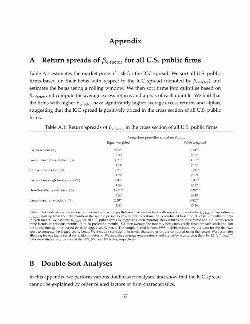
Appendix

A Return spreads of βc-factor for all U.S. public firms

Table A.1 estimates the market price of risk for the ICC spread. We sort all U.S. publicfirms based on their betas with respect to the ICC spread (denoted by βc-factor) andestimate the betas using a rolling window. We then sort firms into quintiles based onβc-factor and compute the average excess returns and alphas of each quintile. We find thatthe firms with higher βc-factor have significantly higher average excess returns and alphas,suggesting that the ICC spread is positively priced in the cross section of all U.S. publicfirms.

Table A.1: Return spreads of βc-factor in the cross section of all U.S. public firms

Long-short portfolios sorted on βc-factor

Equal weighted Value weighted

Excess returns (%) 2.04∗∗ 4.10∗∗∗

[2.02] [2.72]

Fama-French three-factor α (%) 1.75∗ 4.13∗∗

[1.71] [2.22]

Carhart four-factor α (%) 2.25∗ 5.21∗∗

[1.92] [2.59]

Pástor-Stambaugh five-factor α (%) 2.08∗ 5.03∗∗

[1.87] [2.32]

Hou-Xue-Zhang q-factor α (%) 3.45∗∗∗ 9.28∗∗∗

[3.30] [3.49]

Fama-French five-factor α (%) 2.20∗∗ 8.82∗∗∗

[2.00] [3.26]

Note: This table shows the excess returns and alphas for portfolios sorted on the beta with respect to the c-factor (βc-factor). We estimateβc-factor starting from the 13th month of the sample period to ensure that the estimation is conducted based on at least 12 months of data.In each month, we estimate βc-factor for all U.S. public firms by regressing their monthly stock returns on the c-factor and the Fama-Frenchthree factors in previous months up to 36 preceding months. We then average the monthly betas into yearly betas for each stock and sortthe stocks into quintiles based on their lagged yearly betas. The sample period is from 1995 to 2016, because we use data for the first twoyears to compute the lagged yearly betas. We include t-statistics in brackets. Standard errors are computed using the Newey-West estimatorallowing for one lag of serial correlation in returns. We annualize average excess returns and alphas by multiplying them by 12. *, **, and ***indicate statistical significance at the 10%, 5%, and 1% levels, respectively.

B Double-Sort Analyses

In this appendix, we perform various double-sort analyses, and show that the ICC spreadcannot be explained by other related factors or firm characteristics.

57

Controlling for the Measures of Customer Capital. We show that other measures ofcustomer capital are either not priced in the cross section or their association with stockreturns can be explained away by the ICC. Specifically, we study three measures ofcustomer capital: brand stature, brand strength, and firms’ product market fluidity (seeHoberg, Phillips and Prabhala, 2014). We find that none of the three measures are pricedin the cross section after controlling for the ICC (see Online Appendix Table OA.12). Onthe other hand, the ICC remains priced in the cross section after controlling for the threemeasures (see Online Appendix Table OA.13). These findings suggest that studying thedegree to which customer capital depends on key talents is essential to understandingthe role of customer capital in explaining cross-sectional stock returns.

Controlling for the Measures of Intangible Assets. We show that the average excessreturns and alphas of the ICC spread remain significantly positive after controlling forvarious proxies of intangible assets (see Online Appendix Table OA.14). In addition, wefind that the ICC spread is much more robust in firms that have high administrativeexpenses and R&D expenditures (see Online Appendix Table OA.15), suggesting aninteraction effect between the ICC and intangible assets. This result is reminiscent ofthe findings of Li (2011), who documents that the return spread of financial constraintsmeasures is much stronger in R&D intensive firms.

Controlling for Industry Classi�cations. We find that the long-short portfolios sortedon ICC within industries have positive alphas, that are both statistically and economicallysignificant (see Online Appendix Table OA.16). The return patterns are robust acrossvarious industry classifications, suggesting that the ICC’s within-industry variation ispriced in the cross section.

C More Tests for the Theoretical Mechanism

In this section, we provide two sets of additional empirical evidence to support our model.First, we show that the firms with higher ICC adopt more precautionary financial policies.Second, we show that key talents receive lower compensation in firms with greater brandstature. This finding supports our extended model’s assumption that key talents receivenon-pecuniary private benefits from customer capital.

58

Table C.2: The ICC and firms’ financial policies

(1) (1’) (2) (2’) (3) (3’) (4) (4’) (5) (6)Casht

Assett−1(%) ∆Casht

Net incomet(%)

∆EquitytAssett−1

(%)PayouttAssett−1

(%) DividendtAssett−1

(%)Repurchasest

Assett−1(%)

Data Model Data Model Data Model Data Model Data Dataln(ICC)t−1 3.475∗∗∗ 2.238∗∗∗ 9.421∗∗ 1.904∗∗∗ 0.665∗ 0.350∗∗∗ −0.903∗∗∗−0.545∗∗∗ −0.310∗∗∗ −0.591∗∗∗

[5.786] [8.672] [2.219] [4.872] [1.928] [7.354] [−4.457] [−3.985] [−3.111] [−3.934]Firm controls Yes Yes Yes Yes Yes YesIndustry FEs and year FEs Yes Yes Yes Yes Yes YesObservations 5842 5000 4958 5000 5842 5000 5842 5000 5842 5842R-squared 0.439 0.242 0.032 0.015 0.106 0.010 0.296 0.142 0.349 0.248

Note: This table shows the relation between the ICC and firms’ financial policies. The dependent variables are the amount of cashholdings (% of lagged assets), the change in cash holdings (% of contemporaneous net income), the amount of equity issuance (% oflagged assets), the amount of total payout (% of lagged assets), the amount of dividend issuance (% of lagged assets), and the amountof share repurchases (% of lagged assets). The outcome variables are winsorized at the 1st and 99th percentiles of their empiricaldistributions to mitigate the effect of outliers. In column (2), we include only observations with positive net income. The mainindependent variable is lagged standardized ln(ICC). Firm controls include the natural log of market capitalization, the naturallog of the book-to-market ratio, the natural log of the debt-to-equity ratio, and the natural log of organization capital normalizedby assets. The sample period spans 1993 - 2016. We include t-statistics in brackets. Standard errors are clustered by firm andyear. Columns (1’-4’) present the regression coefficient based on the simulated data of our calibrated extended model. *, **, and ***indicate statistical significance at the 10%, 5%, and 1% levels, respectively.

C.1 Low-ICC Firms Adopt More Precautionary Financial Policies

Table C.2 examines the relation between the ICC and firms’ financial policies. We findthat high-ICC firms hold more cash and convert a larger fraction of net income to cashholdings. High-ICC firms also issue more equity and pay out less dividend. Our empiricalfindings are roughly quantitatively consistent with the implications of our model.

C.2 Brand Stature and Private Benefits

In this appendix, we show that the private benefits of key talents increase with totalcustomer capital. Specifically, we show that executives are willing to accept lower payfrom firms with higher brand stature, a proxy for total customer capital.31 The relationbetween brand stature and executive pay is economically significant. According to theregression with executive fixed effects, industry fixed effects, and year fixed effects, aone-standard-deviation increase in brand stature is associated with a 10.8% reduction inmanagerial compensation (see column 4 of Table C.3). In addition, we find that youngerexecutives are more likely to enjoy non-pecuniary private benefits at the firms with strong

31Our findings are consistent with the literature. In a laboratory setting, researchers find that undergrad-uate students are willing to accept lower hypothetical salaries from the firms with higher reputation (see,e.g., Gatewood, Gowan and Lautenschlager, 1993; Cable and Turban, 2003). Using BAV and Execucompdata from 2000 to 2010, Tavassoli, Sorescu and Chandy (2014) show that CEOs and top executives arewilling to accept lower pay from firms with stronger brand value.

59

Table C.3: Brand stature and talents’ non-pecuniary private benefits

(1) (2) (3) (4) (5) (6)

lnExecuCompt

lnStaturet−1 −0.096∗∗∗ −0.063∗∗ −0.113∗∗ −0.108∗∗ −0.173∗∗∗ −0.158∗∗∗

[−4.002] [−2.704] [−2.524] [−2.303] [−3.542] [−3.561]

lnStaturet−1 × (Aget−1 − 30) 0.003∗ 0.004∗∗

[1.747] [2.306]

lnStrengtht−1 0.057∗ 0.015 0.053∗ 0.055∗ 0.026 −0.009

[2.035] [0.519] [1.863] [1.859] [0.307] [−0.122]

lnStrengtht−1 × (Aget−1 − 30) 0.001 0.001

[0.412] [0.350]

Aget−1 0.019∗∗∗ 0.019∗∗∗ −0.137∗∗∗ −0.152∗∗∗ 0.018∗∗∗ 0.018∗∗∗

[5.365] [6.125] [−5.195] [−4.655] [5.786] [6.690]

Firm controls Yes Yes Yes Yes Yes Yes

Executive controls Yes Yes No No Yes Yes

Executive FEs No No Yes Yes No No

Industry FEs No Yes No Yes No Yes

Year FEs Yes Yes Yes Yes Yes Yes

Observations 23496 23496 22267 22267 23496 23496

R-squared 0.283 0.299 0.748 0.749 0.283 0.299

Note: This table shows the relation between brand value and managerial compensation. lnExecuComp is the natural log of themanagerial compensation (tdc1 in the Execucomp data). We standardize both lnStature and lnStrength to ease the interpretationof coefficients. Firm controls include the natural log of firm market capitalization, the natural log of the book-to-market ratio, thenatural log of the debt-to-equity ratio, the natural log of organization capital normalized by assets, and the stock returns in theprevious year. We also include executive genders as executive controls in the specifications without executive fixed effects. Thesample period spans 1993 - 2016. We include t-statistics in brackets. Standard errors are clustered by firm and year. *, **, and ***indicate statistical significance at the 10%, 5%, and 1% levels, respectively.

brand stature. According to the specification with both industry and year fixed effects(see column 6 of Table C.3), a 30-year-old executive is willing to take a 15.8% cut incompensation with a one-standard-deviation increase in the brand stature of the firm,whereas a 67-year-old executive is not willing to accept any compensation cut.

60