current developments of remote sensing for mapping and

Current developments of remote sensing for mapping and monitoring land degradation at regional scale

Prof Graciela MetternichtChair, ICA Commission on Mapping from Satellite Imagery

Curtin University of TechnologyPerth, Western Australia

Email: [email protected]

UN-Zambia-ESA Regional Workshop on the Applications of GNSS in Sub-Saharan Africa

June 2006

UNOOSA – ESA Regional Workshop, Zambia, June 2006 2

What is land degradation?

Land degradation is the reduction in the capability of the land to produce benefits from a particular land use under a specified form of land management (after Blaikie and Brookfield 1987). Soil degradation is one aspect of land degradation; others are degradation of vegetation or water resources.


Processes of land degradationLand degradation results in adverse effects of which we like to know the spatial and temporal variation.Knowledge of:processes of land degradation, and hence the process-controlling variables, and the effects of degradation is a pre-requisite to determine which variables can be derived from remotely sensed images.


The Scale FactorFactors controlling spatial variation of land degradation depend on scale.Macro-scale: 1:1,000,000

climate is considered a very important factorMicro-scale: 1:50,000 and finer scales

Climate is fairly uniformVariation of soil propertiesLithologyTopographyVegetation properties, become important


The scale factor (cont)At micro-scale the short distance spatial variability of process-controlling factors becomes important.Using vegetation or soil maps with large mapping units doesn’t make sense, as local variation has to be captured.Remote sensing can play an important role in capturing local variation


Methods for assessing land degradation

Expert opinion: subjective assessment, using semi-quantitative definitions (e.g. GLASOD survey)Remote sensing: satellite and airborne images, linked to ground observations. Ground-based radiometryField observations: including stratified soil sampling and analysis, long term field observations of vegetation and biodiversity in specific sites.


Methods for land degradation assessment (cont.)

Productivity changes: observing changes in crop yieldLand users opinions and farm level field criteria: studies at farm level are seen as essential on a sample basis, to obtain a view of the severity of degradation and its causes, together with practicable remedial measuresModelling: based on data obtained by other methods, modelling is applied for:

Prediction of hazard to degradation (GIS-based models)Extending the range of applicability of results on observed degradation.

None of these consist in a single methodology, synergistic use (e.g. Combined approaches) are common.


Mapping and modelling land degradation

Satellite imagery and aerial photographs are recommended tools for:1. Assessing the spatial and temporal

distribution of land degradation features;2. Collecting input data for process simulation

models in order to produce land cover maps, vegetation cover maps, bare soil fraction maps, etc


1. Assessing spatial and temporal distributionSurveying: to assess the current status of the land in terms of ongoing degradation processes. Aims:

Determining the spatial variability and statusof:

Natural vegetation (coverage and structure)Agricultural crops (performance, coverage)Soil surface (e.g. sealing or crusting)Presence of soil erosion surface features (gullies, rills)

Monitoring changes over time:Development of crop canopy over a growing season (indicator of erosion)Long term development of rill and gully formation in an area.


Detecting and measuring indicators: Techniques

Indicators can be detected using a variety of techniques, including

Field observations (GPS), Laboratory analysis, Remotely sensed data or a combination thereof.


2. Input data for modelling

Process controlling variables such as:rainfall interception, water canopy storage and changing agricultural land use through the growing season are derived from air- or satellite-borne images to use the information in process simulation models.


Land degradation processes/ remote sensing requirements: temporal and spatial

Low spatial resolutionHigh temporal resolution

High spatial resolutionLow temporal resolution

Low spatial resolutionLow temporal resolution

High spatial resolutionHigh Temporal resolution

Fast changes Slow changes

Changes over extensive areas (regional scale)

Changes over small areas (local scale)

Land degradation mapping and monitoring

Factors influencing the use of RS as a mapping tool

Sensors and platforms commonly used


Factors affecting feature discrimination and mapping

The one-to-many relationship between surface features and land degradation processes, one feature characterising many degradation process (Figure 1);The spectral similarity among surface component associated with land degradation; and The differences in spatial resolution of various data sources used for mapping purposes, including remotely sensed data, field observations and laboratory determinations.


Constraints on the use of remote sensing: land salinization example

Salts at the terrain surface can be detected from remotely sensed data:

Directly: salt efflorescences, salt crusts, bare soilsIndirectly: through vegetation type and growth; vegetation health’s status

Remote Sensing Sources: soil salinity as a form of land degradation

SatelliteAirborne

Ground-based

Sources of remote sensing dataSatellite-borne sensors Sensor No of bands Spectral Range (µm) Spatial resolution

Visible, NIR, mid- and thermal infrared B1: 0.45-0.52 B2: 0.52-0.60 B3:0.63-0.69 B4:0.76-0.90 B5: 1.55-1.75 B6: 10.40-12.50 B7: 2.08-2.35

Landsat TM4&5 Landsat TM7-ETM+

7 ( 1-7) 8 (1-8)

B8: 0.52-0.90 (pan)

Bands 1-5 and 7: 30 m Band 6: 120m Band 8: 15m

Visible, NIR Xs1: 0.50-0.59 Xs2: 0.61-0.68 Xs3: 0.79-0.89 Xi4: 1.58-1.75 Pan:0.51-0.73

SPOT 1-3

SPOT 4

4 (Xs1-3 & Pan)

5 (Xi1-4 and Mono)

Mono:0.61-0.68

Xs or Xi: 20 m Pan and Mono: 10 m

Visible, NIR, mid-infrared B1: 0.52 - 0.59 B2: 0.62 - 0.68 B3: 0.77 - 0.86

LISS-III 4

B4: 1.55 - 1.70

Bands 1-3: 23 m Band 4: 70 m

Visible, NIR B1: 0.45-0.52 B2: 0.52-0.59 B3: 0.62-0.68

LISS-II 4

B4: 0.77-0.86

36.25m

IRS-1C 1 0.5-0.75 (pan) 5.8m JERS-1 1 Microwave 18-12.5 m

Airborne sensors Aerial photographs B/W; colour infrared variable, depending on

flight height Visible, NIR 0.54-0.55 0.64-0.65

Narrow-band videography

3

0.84-0.85

3.4 m

Visible, NIR 0.44-0.46 0.54-0.56 0.64-0.66

DMSV (Digital Multispectral Video Systems)

4

0.74-0.76

variable: 0.25m-2m

Microwave (full polarimetric) AIRSAR-TOPSAR 3P-, L- and C-bands

10m

Visible, NIR, mid-infrared Hyperspectral Hymap

1280.45 - 2.5

2- 10 m

0.4 - 12 0.4-1 (32 bands) 1.5-1.8 (8 bands) 2 - 2.5 (32 bands) 3 - 5 (1 band)

Hyperspectral DAIS-7915

79

8.5 - 12.3 (6 bands)

3 - 20 m

gravity magnetic electromagnetic

Airborne geophysics

gramma-ray


Mission Launch Year

Instrument Spatial Resolution (meters, at nadir) Swath • (km)

PAN* VNIR* SWIR* TIR* SAR*/ band

Repeat Cycle (day)

Landsat 5 1984 TM 30 30 120 185 16 SPOT-2 1990 HRV 10 20 60 1 to 26 ERS-1 1991 AMI-SAR 30/C 100 16-35 ATSR-1 1000 1000 50000 500 16-35 IRS-1B 1991 LISS I 72 148 22 LISS 2 36 74x2 22 IRS-P2 1994 LISS 2 36 132 24 Resurs-O1 N3 1994 MSU-SK 170 600 600 2 to 4 ERS-2 1995 AMI-SAR 30/C 100 16-35 ATSR-2 1000 1000 50000 500 16-35 IRS-1C 1995 PAN 6 70 5 to 24 LISS 3 23 70 142-148 24 1995 WiFS 188 188 774 5 to 24 Radarsat 1995 SAR 10-100/C 45-500 4 to 6 IRS-P3 1996 MOS 500 200 5 WiFS 188 188 770 5 IRS-1D 1997 PAN 6 70 5 to 24 LISS 3 23 70 142-148 24 WiFS 188 188 774 5 to 24 SPOT-4 1998 2xHRV-IR 10 10, 20 10, 20 60 3 Vegetation 1000 1000 2200 1 Landsat 7 1999 ETM+ 15 30 30 30 185 16 Ikonos 1999 Ikonos 1 4 11 3 CBERS 1999 CCD 20 20 20 120 3 to 26 IR-MSS 80 80 80 120 26 WFI 260 260 900 3 to 5 Terra (EOS AM-1) 1999 ASTER 15 20 90 60 16 MISR 240, 480,

960, 1900 370-408 2 to 9

MODIS 250, 500, 1000

500, 1000

1000 2300 2

Quickbird 2 2001 Quickbird 0.6 4 22 1 to 5

ADEOS-2 2002 GLI 250 250 1000 1600 4 Aqua (EOS PM-1) 2002 MODIS 250, 500,

1000 500, 1000

1000 2300 2

ENVISAT-1 2002 AATSR 1000 1000 1000 512 3 ASAR 30/C 100 3 SPOT-5a 2002 HRG 5 10 20 60 3 Vegetation 1000 1000 2200 1


Forthcoming High ResolutionIRS-P5 (CartoSat-1)

PAN-F 2.5 30 5 2005

35(70) ALOS PRISM, AVNIR-2

2.510(4)

70

46(2) 2005

MUX 20 (4) 120 26 2008 PAN 5 60 1 - 26 2011 ISR 40 40 (2) 80 120 26

CBERS 3 & 4

WFI 73 (4)

866 5 TopSat2 RALCam1 2.5 5 (3) 25 4 2005

Plèiades3–1 & 2 HiRI 0.7 2.8 (4) 20 26 to 4 2008-2009

RapidEye A-E4 REIS 6.5 6.5 (5) 78 1 2007

EROS B - C PIC 0.7 2.8 11 2005-2008

RazakSat5 MAC 2.5 5 (4) 20 13-157 2005China DMC+4 (Tsinghua-1)

MS DMC 4 32 (3) 600 2005

Resurs DK-16 ESI 1 3 (3) 28.3 N/A 20051DMC (Disaster Monitoring Constellation of 4 satellites) of sun-synchronic circular orbit, daily revisit cycle. 2 Circular, sun-synchronic orbit 3 two-spacecraft constellation of CNES (Space Agency of France), with provision of stereo images. 4 five-satellite constellation 5 near equatorial low Earth orbit (NEO) 6 Near-circular non-sun synchronous orbit 7 passes/day

Spatial Res o lution (meters ) and (# Bands ) Optical Sate llite

Sens or PAN VNIR SWIR MWIR TIR

Swath (Km)

Repeat Cyc le

Year Launch


Ground-based sensors Electromagnetic induction meter (EM38, EM31, EM34-3, EM39)

Electromagnetic conductivity meters, measures the bulk electrical conductivity of soils

Crop Scan multi-band radiometer (Skye Instruments Ltd, UK)

8 Visible, NIR

Sources of Remote Sensing data


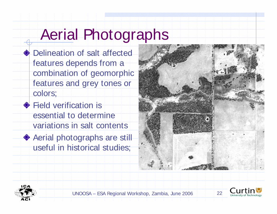
Aerial PhotographsDelineation of salt affected features depends from a combination of geomorphic features and grey tones or colors;Field verification is essential to determine variations in salt contentsAerial photographs are still useful in historical studies;


Airborne Videography & Digital Multispectral cameras

It presents the advantages of:High spatial resolutionNear real time data acquisitionDigital multispectral images

Previous studies have demonstrated good correlations between spectral variations and the response of cotton to soil salinity, in the range of the blue to NIRFor salt affected areas, colour infrared composites and red narrow band images have proven better than green and NIR bands.


Microwave SensingRelatively few studies have investigated the possibility of using microwave for mapping areas degraded by salinizationC-, P- and L- bands are considered adequate for detecting salinity Previous studies have focused on the following features:

Saline water detection by analysing the dependence of microwave responses on salinity and temperatureSoil salinity identification by relating salinity levels to the imaginary parts of the complex dielectric constantSoil salinity mapping, including discrimination of salinity levels by mapping surface roughness and vegetation types related to salinityThe info above is then used as ancillary data to estimate the extent of salinity at regional level.


Microwave: backscattering


Forthcoming Satellite SARsSATELLITE3 ERS-1 ERS2 RADARSAT-

1 JERS-1 ENVISAT RADARSAT-

2 ALOS TERRASAR-X COSMO/

SKYMED1

Sensor AMI AMI SAR SAR ASAR SAR PALSAR TSX-1 SAR-2000

Space Agency ESA ESA RadarSat Int

NASDA ESA RadarSat Int

NASDA DLR/Infoterra GmbH

ASI

Operational since

1991 1995 1995 1992 2002 2005 2004 2006 2005

Out of Service Since

2000 1998

Band C C C L C C L X X Wavelength (cm)

5.7 5.7 5.7 23.5 5.7 5.7 23.5 3 3

Polarization VV VV HH HH HH/VV QUAD-Pol*

All All HH/VV

Incidence angle (°)

23 23 20-50 35 15-45 10-60 8-60 15-60 Variable

Resolution range (m)

26 26 10-100 18 30-150 3-100 7-100 1-16 1-100

Resolution azimuth (m)

28 28 9-100 18 30-150 3-100 7-100 1-16 1-100

Scene width (km)

100 100 45-500 75 56-400 50-500 40-350 5-100 (up to 350)

10-200 (up to 1,300)

Repeat cycle (days)

35 35 24 44 35 24 2-46 2-11 5-16

Orbital elevation (km)

785 785 798 568 800 798 660 514 619


Hyperspectral sensing

Experiments carried out using Hymap (128 bands, 450-2500 nm). Mapped: salt scalds halophytic vegetation and soils with varying salinity degrees and types.Visible and NIR: enable detection of features related to hydrated evaporite minerals.


Ground sensing: electromagnetic induction

The EM series (EM 31, EM34-3, EM38, EM39) estimate soil salinity by measuring the bulk electrical conductivity of the soil, which depends on the salinity of the soil solution, porosity and the type and amount of clay in the soil.The instrument measures the apparent soil salinity (ECa) in a volume of soil below the transmitter and receiver coils.EM surveys are a way for rapid diagnosis and mapping of soil salinity. Survey speed depends on terrain conditions, topography and land use.


EM: how it works?

Multi-scale modelling

Integrating remote sensing and GIS for defining areas of priority

of intervention


Modelling at multi-scale level

Multi-level approaches are cost-effective and enable decision maker focussing on areas of high priority of intervention


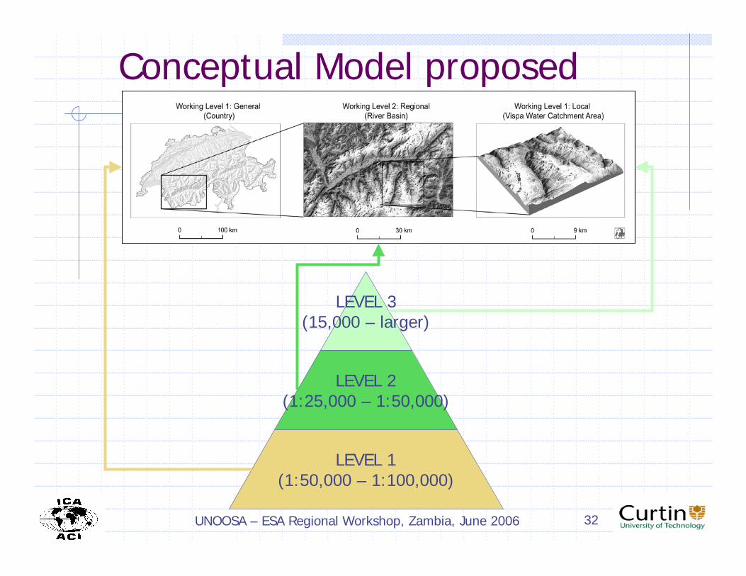
Conceptual Model proposed

LEVEL 3(15,000 – larger)

LEVEL 2(1:25,000 – 1:50,000)

LEVEL 1(1:50,000 – 1:100,000)


The modelLevel 1: Basic detection of diagnostic features over large areas.Sensors: Terra ASTER, Landsat TM, IRS, SPOT, Radarsat, Envisat, ERS.Multi-temporal &/or multi-sensor images can be used for mapping changes of environment-related factors over time.More qualitative assessment: Detect potentially dangerous areas of debris flows and associated hazards.


The modelLevel 2: assess hazard potential or diagnostic features at more detail, over areas identified as potentially dangerous in Level 1.Integrates GIS for analysis.Sensors: VHR satellites, & SPOT-5, IRS CartoSat-1) and satellites with InSAR capabilities.More quantitative assessment: Produce motion maps, etc.


The modelLevel 3: detailed investigations of areas identified in L1 & L2.Sensors: mostly limited to sensors with DInSAR or InSAR capabilities, very high res. Images, LiDAR szstems, Ground based DInSAR.Quantitative assessment: deposits thickness, motion, debris distribution along and across the debris flow deposits.

General conclusions

Perspectives: toolsMODISAstroVision

QuickbirdIkonosSPOT-5

QuickbirdIkonosSPOT-5ASTERCartosat

LandsatRadarsatERSEnvisatASTER

Low spatial resolutionHigh temporal resolution

High spatial resolutionLow temporal resolution

Low spatial resolutionLow temporal resolution

High spatial resolutionHigh Temporal resolution

Fast changes Slow changes

Changes over extensive areas (regional scale)

Changes over small areas (local scale)


Assessing Temporal and Spatial Changes

Monitoring land degradation changes from past to present faces the difficulty that, in general, there is no ground-truth information available for past situations.Consequently, validation of historical remote sensing data involves uncertaintiesFusion of multi-source remote sensing data and their integration with field and laboratory data can overcome part of this problem.


Issues in remote monitoring of land degradation

As salt related surface features change with seasons, time series of remote sensing data must be captured in similar periods of the year, preferably at the end of the dry season if passive remote sensors are used.Geo-referencing and co-registration of multi-temporal data are essentialRadiometric calibration between images so that digital numbers from different dates can be compared, particularly if direct application of a unique ‘training set’ is applied to the images.


Final comments

Regardless the land degradation type mapped and/or monitored, the identification of correct indicators or diagnostic features is essential before any Remote Sensing or GIS modellingare applied.Salinity: monitoring of soil salinity and early warning of salinisation cannot be achieved from remote sensing data alone. It requires synergy between remote sensing, field observations, laboratory analysis, and GISfacilities for processing, displaying, modelling.

current developments of remote sensing for mapping and

Documents