cse 473markov decision processes dan weld many slides from chris bishop, mausam, dan klein, stuart...
TRANSCRIPT

CSE 473 Markov Decision Processes
Dan Weld
Many slides from Chris Bishop, Mausam, Dan Klein, Stuart Russell, Andrew Moore & Luke Zettlemoyer

Logistics
PS 2 due Tuesday Thursday 10/18
PS 3 due Thursday 10/25

MDPs
Markov Decision Processes• Planning Under Uncertainty
• Mathematical Framework• Bellman Equations• Value Iteration• Real-Time Dynamic Programming• Policy Iteration
• Reinforcement Learning
Andrey Markov (1856-1922)

Planning Agent
What action next?
Percepts Actions
Environment
Static vs. Dynamic
Fully vs.
Partially Observable
Perfectvs.
Noisy
Deterministic vs.
Stochastic
Instantaneous vs.
Durative

Objective of an MDP
• Find a policy : S → A
• which optimizes • minimizes expected cost to reach a goal• maximizes expected reward• maximizes expected (reward-cost)
• given a ____ horizon• finite• infinite• indefinite
• assuming full observability
discountedor
undiscount.

Grid World
Walls block the agent’s path Agent’s actions may go astray:
80% of the time, North action takes the agent North (assuming no wall)
10% - actually go West 10% - actually go East If there is a wall in the chosen
direction, the agent stays put Small “living” reward each step Big rewards come at the end Goal: maximize sum of rewards

Markov Decision Processes An MDP is defined by:
• A set of states s S• A set of actions a A• A transition function T(s,a,s’)
• Prob that a from s leads to s’• i.e., P(s’ | s,a)• Also called “the model”
• A reward function R(s, a, s’) • Sometimes just R(s) or R(s’)
• A start state (or distribution)• Maybe a terminal state
• MDPs: non-deterministic search Reinforcement learning: MDPs where we don’t know the transition or reward functions

What is Markov about MDPs?
Andrey Markov (1856-1922)
“Markov” generally means that • conditioned on the present state, • the future is independent of the past
For Markov decision processes, “Markov” means:

Solving MDPs
In an MDP, we want an optimal policy *: S → A• A policy gives an action for each state• An optimal policy maximizes expected utility if followed• Defines a reflex agent
Optimal policy when R(s, a, s’) = -0.03
for all non-terminals s
In deterministic single-agent search problems, want an optimal plan, or sequence of actions, from start to a goal

Example Optimal Policies
R(s) = -2.0R(s) = -0.4
R(s) = -0.03R(s) = -0.01

Example Optimal Policies
R(s) = -2.0R(s) = -0.4
R(s) = -0.03R(s) = -0.01

Example Optimal Policies
R(s) = -2.0R(s) = -0.4
R(s) = -0.03R(s) = -0.01

Example Optimal Policies
R(s) = -2.0R(s) = -0.4
R(s) = -0.03R(s) = -0.01
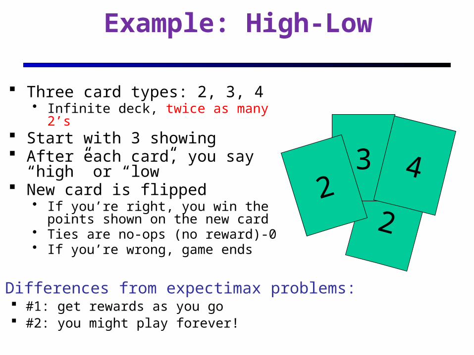
Example: High-Low
Three card types: 2, 3, 4• Infinite deck, twice as many 2’s
Start with 3 showing After each card, you say “high”
or “low” New card is flipped
• If you’re right, you win the points shown on the new card
• Ties are no-ops (no reward)-0• If you’re wrong, game ends
2
32
4
Differences from expectimax problems: #1: get rewards as you go #2: you might play forever!

High-Low as an MDP States:
• 2, 3, 4, done Actions:
• High, Low Model: T(s, a, s’):
• P(s’=4 | 4, Low) = • P(s’=3 | 4, Low) = • P(s’=2 | 4, Low) = • P(s’=done | 4, Low) = 0• P(s’=4 | 4, High) = 1/4 • P(s’=3 | 4, High) = 0• P(s’=2 | 4, High) = 0• P(s’=done | 4, High) = 3/4• …
Rewards: R(s, a, s’):• Number shown on s’ if s’<s a=“high” …• 0 otherwise
Start: 3
2
32
41/41/4
1/2

Search Tree: High-Low
3Low High
2 43High Low High Low High Low
3 , Low , High3
T = 0.5, R = 2
T = 0.25, R = 3
T = 0, R = 4
T = 0.25, R = 0

MDP Search Trees Each MDP state gives an expectimax-like search
tree
a
s
s’
s, a(s,a,s’) called a transition
T(s,a,s’) = P(s’|s,a)
R(s,a,s’)
s,a,s’
s is a state
(s, a) is a q-state

Utilities of Sequences
In order to formalize optimality of a policy, need to understand utilities of sequences of rewards
Typically consider stationary preferences:
Theorem: only two ways to define stationary utilities Additive utility:
Discounted utility:

Infinite Utilities?!
Problem: infinite state sequences have infinite rewards
Solutions:• Finite horizon:
• Terminate episodes after a fixed T steps (e.g. life)• Gives nonstationary policies ( depends on time left)
• Absorbing state: guarantee that for every policy, a terminal state will eventually be reached (like “done” for High-Low)
• Discounting: for 0 < < 1
• Smaller means smaller “horizon” – shorter term focus

Discounting
Typically discount rewards by < 1 each time step• Sooner rewards
have higher utility than later rewards
• Also helps the algorithms converge

Recap: Defining MDPs
Markov decision processes:• States S• Start state s0• Actions A• Transitions P(s’|s, a)
aka T(s,a,s’)• Rewards R(s,a,s’) (and discount )
MDP quantities so far:• Policy, = Function that chooses an action for each
state• Utility (aka “return”) = sum of discounted rewards
a
s
s, a
s,a,s’s’

Optimal Utilities
Define the value of a state s:V*(s) = expected utility starting in s and
acting optimally Define the value of a q-state (s,a):
Q*(s,a) = expected utility starting in s, taking action a and thereafter acting optimally
Define the optimal policy:*(s) = optimal action from state s
a
s
s, a
s,a,s’s’

Why Not Search Trees?
Why not solve with expectimax?
Problems:• This tree is usually infinite (why?)• Same states appear over and over
(why?)• We would search once per state
(why?)
Idea: Value iteration• Compute optimal values for all states
all at once using successive approximations
• Will be a bottom-up dynamic program similar in cost to memoization
• Do all planning offline, no replanning needed!

The Bellman Equations
Definition of “optimal utility” leads to a simple one-step look-ahead relationship between optimal utility values:
(1920-1984)
a
s
s, a
s,a,s’s’

Bellman Equations for MDPs
Q*(a, s)

Bellman Backup (MDP)
• Given an estimate of V* function (say Vn)• Backup Vn function at state s
• calculate a new estimate (Vn+1) :
• Qn+1(s,a) : value/cost of the strategy:• execute action a in s, execute n subsequently• n = argmaxa∈Ap(s)Qn(s,a)
V
R V
ax
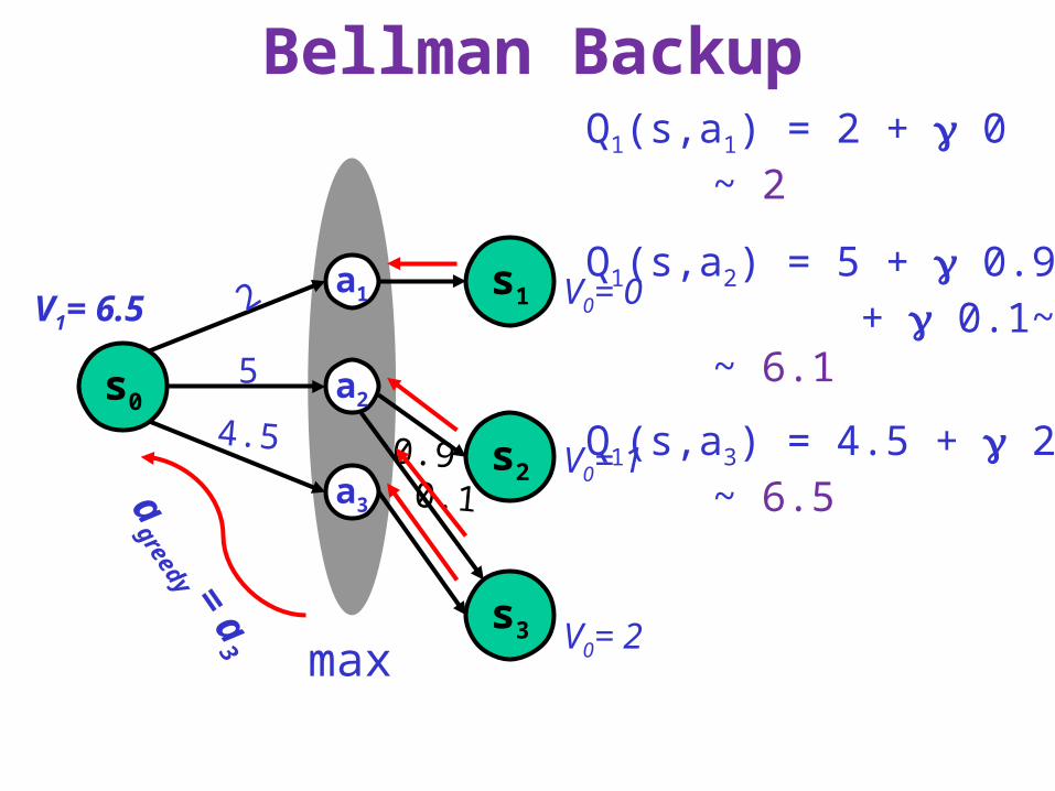
Bellman Backup
V0= 0
V0= 1
V0= 2
Q1(s,a1) = 2 + 0 ~ 2
Q1(s,a2) = 5 + 0.9~ 1 + 0.1~ 2 ~ 6.1
Q1(s,a3) = 4.5 + 2 ~ 6.5
max
V1= 6.5
agreed
y = a
3
2
4.5
5 a2
a1
a3
s0
s1
s2
s3
0.90.1

Value iteration [Bellman’57]
• assign an arbitrary assignment of V0 to each state.
• repeat• for all states s
• compute Vn+1(s) by Bellman backup at s.
• until maxs |Vn+1(s) – Vn(s)| <
Iteration n+1
Residual(s)
Theorem: will converge to unique optimal values Basic idea: approximations get refined towards optimal values Policy may converge long before values do
-convergence

Example: Bellman UpdatesExample: γ=0.9, living reward=0, noise=0.2
?
?
? ???
?
? ?

Example: Value Iteration
Information propagates outward from terminal states and eventually all states have correct value estimates
V1 V2

Example: Value Iteration
QuickTime™ and aGIF decompressor
are needed to see this picture.

Practice: Computing Actions
Which action should we chose from state s:
• Given optimal values Q?
• Given optimal values V?
• Lesson: actions are easier to select from Q’s!

Convergence
Define the max-norm:
Theorem: For any two approximations Ut and Vt
• I.e. any distinct approximations must get closer to each other, so, in particular, any approximation must get closer to the true V* (aka U) and value iteration converges to a unique, stable, optimal solution
Theorem:
• I.e. once the change in our approximation is small, it must also be close to correct

Value Iteration Complexity
Problem size: • |A| actions and |S| states
Each Iteration• Computation: O(|A|⋅|S|2)• Space: O(|S|)
Num of iterations• Can be exponential in the discount
factor γ

MDPs
Markov Decision Processes• Planning Under Uncertainty
• Mathematical Framework• Bellman Equations• Value Iteration• Real-Time Dynamic Programming• Policy Iteration
• Reinforcement Learning
Andrey Markov (1856-1922)

Asynchronous Value Iteration
States may be backed up in any order• Instead of systematically, iteration by iteration
Theorem: • As long as every state is backed up infinitely often…• Asynchronous value iteration converges to optimal

Asynchonous Value Iteration Prioritized Sweeping
Why backup a state if values of successors same? Prefer backing a state
• whose successors had most change
Priority Queue of (state, expected change in value) Backup in the order of priority After backing a state update priority queue
• for all predecessors

Asynchonous Value IterationReal Time Dynamic Programming
[Barto, Bradtke, Singh’95]
• Trial: simulate greedy policy starting from start state; perform Bellman backup on visited states
• RTDP: • Repeat Trials until value function converges

Why?
Why is next slide saying min

Min
?
?s0
Vn
Vn
Vn
Vn
Vn
Vn
Vn
Qn+1(s0,a)
Vn+1(s0)
agreedy = a2
RTDP Trial
Goala1
a2
a3
?

Comments
• Properties• if all states are visited infinitely often then Vn → V*
• Advantages• Anytime: more probable states explored quickly
• Disadvantages• complete convergence can be slow!

Labeled RTDP Stochastic Shortest Path Problems
• Policy w/ min expected cost to reach goal Initialize v0(s) with admissible heuristic
• Underestimates remaining cost Theorem:
• if residual of Vk(s) < e and Vk(s’) < e for all succ(s), s’, in greedy graph• Then Vk is e-consistent and will remain so
Labeling algorithm detects convergence
?s0
Goal
[Bonet&Geffner ICAPS03]

MDPs
Markov Decision Processes• Planning Under Uncertainty
• Mathematical Framework• Bellman Equations• Value Iteration• Real-Time Dynamic Programming• Policy Iteration
• Reinforcement Learning
Andrey Markov (1856-1922)

Changing the Search Space
• Value Iteration• Search in value space• Compute the resulting policy
• Policy Iteration• Search in policy space• Compute the resulting value

Utilities for Fixed Policies
Another basic operation: compute the utility of a state s under a fix (general non-optimal) policy
Define the utility of a state s, under a fixed policy p:Vp(s) = expected total
discounted rewards (return) starting in s and following p
Recursive relation (one-step look-ahead / Bellman equation):
p(s)
s
s, p(s)
s, p(s),s’
s’

Policy Evaluation
How do we calculate the V’s for a fixed policy?
Idea one: modify Bellman updates
Idea two: it’s just a linear system, solve with Matlab (or whatever)

Policy Iteration
Problem with value iteration:• Considering all actions each iteration is slow: takes |A|
times longer than policy evaluation• But policy doesn’t change each iteration, time wasted
Alternative to value iteration:• Step 1: Policy evaluation: calculate utilities for a fixed
policy (not optimal utilities!) until convergence (fast)• Step 2: Policy improvement: update policy using one-
step lookahead with resulting converged (but not optimal!) utilities (slow but infrequent)
• Repeat steps until policy converges
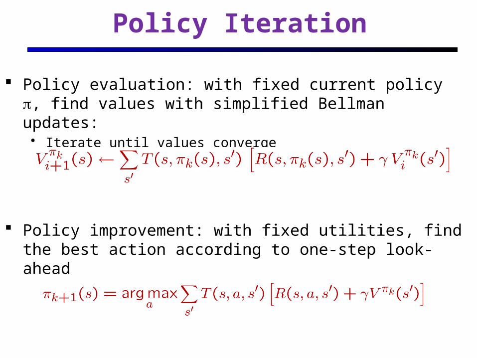
Policy Iteration
Policy evaluation: with fixed current policy p, find values with simplified Bellman updates:• Iterate until values converge
Policy improvement: with fixed utilities, find the best action according to one-step look-ahead

Policy iteration [Howard’60]
• assign an arbitrary assignment of 0 to each state.
• repeat• Policy Evaluation: compute Vn+1: the evaluation of n
• Policy Improvement: for all states s• compute n+1(s): argmaxa2 Ap(s)Qn+1(s,a)
• until n+1 = n
Advantage
• searching in a finite (policy) space as opposed to uncountably infinite (value) space ⇒ convergence faster.
• all other properties follow!
costly: O(n3)
approximateby value iteration using fixed policy
Modified Policy Iteration

Modified Policy iteration
• assign an arbitrary assignment of 0 to each state.
• repeat• Policy Evaluation: compute Vn+1 the approx. evaluation of n
• Policy Improvement: for all states s• compute n+1(s): argmaxa2 Ap(s)Qn+1(s,a)
• until n+1 = n
Advantage
• probably the most competitive synchronous dynamic programming algorithm.

Policy Iteration Complexity
Problem size: • |A| actions and |S| states
Each Iteration• Computation: O(|S|3 + |A|⋅|S|2)• Space: O(|S|)
Num of iterations• Unknown, but can be faster in practice• Convergence is guaranteed

Comparison
In value iteration:• Every pass (or “backup”) updates both utilities (explicitly,
based on current utilities) and policy (possibly implicitly, based on current policy)
In policy iteration:• Several passes to update utilities with frozen policy• Occasional passes to update policies
Hybrid approaches (asynchronous policy iteration):• Any sequences of partial updates to either policy entries or
utilities will converge if every state is visited infinitely often

Recap: MDPs
Markov decision processes:• States S• Actions A• Transitions P(s’|s,a) (or T(s,a,s’))• Rewards R(s,a,s’) (and discount γ)• Start state s0
Quantities:• Returns = sum of discounted rewards• Values = expected future returns from a state
(optimal, or for a fixed policy)• Q-Values = expected future returns from a q-
state (optimal, or for a fixed policy)
a
s
s, a
s,a,s’s’