CSCI 3104 Algorithms- Lecture Notes

Michael Levet

October 19, 2021

Contents

1 Proof by Induction 31.1 Supplemental Reading . . . . . . . . . . . . . . . . . . . . . . . . . . . . . . . . . . . . . . . . . 6

2 Graph Traversals 72.1 Depth-First Traversal . . . . . . . . . . . . . . . . . . . . . . . . . . . . . . . . . . . . . . . . . 72.2 Breadth-First Traversal . . . . . . . . . . . . . . . . . . . . . . . . . . . . . . . . . . . . . . . . 122.3 Shortest-Path Problem: Unweighted Graphs . . . . . . . . . . . . . . . . . . . . . . . . . . . . . 142.4 Shortest-Path Problem: Weighted Graphs and Dijkstra’s Algorithm . . . . . . . . . . . . . . . 17

2.4.1 Dijkstra’s Algorithm: Example 1 . . . . . . . . . . . . . . . . . . . . . . . . . . . . . . . 182.4.2 Dijkstra’s Algorithm: Example 2 . . . . . . . . . . . . . . . . . . . . . . . . . . . . . . . 22

2.5 Dijkstra’s Algorithm: Proof of Correctness . . . . . . . . . . . . . . . . . . . . . . . . . . . . . . 272.6 Supplemental Reading . . . . . . . . . . . . . . . . . . . . . . . . . . . . . . . . . . . . . . . . . 29

3 Greedy Algorithm Principles 303.1 Exchange Arguments . . . . . . . . . . . . . . . . . . . . . . . . . . . . . . . . . . . . . . . . . . 30

3.1.1 Supplemental Reading . . . . . . . . . . . . . . . . . . . . . . . . . . . . . . . . . . . . . 303.2 Interval Scheduling . . . . . . . . . . . . . . . . . . . . . . . . . . . . . . . . . . . . . . . . . . . 31

3.2.1 Supplemental Reading . . . . . . . . . . . . . . . . . . . . . . . . . . . . . . . . . . . . . 333.3 Example Where the Greedy Algorithm Yields Sub-Optimal Solutions . . . . . . . . . . . . . . . 34

4 Spanning Trees 374.1 Preliminaries: Trees . . . . . . . . . . . . . . . . . . . . . . . . . . . . . . . . . . . . . . . . . . 374.2 Safe and Useless Edges . . . . . . . . . . . . . . . . . . . . . . . . . . . . . . . . . . . . . . . . . 404.3 Kruskal’s Algorithm . . . . . . . . . . . . . . . . . . . . . . . . . . . . . . . . . . . . . . . . . . 45

4.3.1 Kruskal’s Algorithm: Proof of Correctness . . . . . . . . . . . . . . . . . . . . . . . . . . 484.3.2 Kruskal’s Algorithm: Runtime Complexity . . . . . . . . . . . . . . . . . . . . . . . . . 50

4.4 Prim’s Algorithm . . . . . . . . . . . . . . . . . . . . . . . . . . . . . . . . . . . . . . . . . . . . 514.4.1 Prim’s Algorithm: Example 1 . . . . . . . . . . . . . . . . . . . . . . . . . . . . . . . . . 524.4.2 Prim’s Algorithm: Example 2 . . . . . . . . . . . . . . . . . . . . . . . . . . . . . . . . . 554.4.3 Algorithm 7 Correctly Implements Prim’s Algorithm . . . . . . . . . . . . . . . . . . . . 594.4.4 Prim’s Algorithm: Proof of Correctness . . . . . . . . . . . . . . . . . . . . . . . . . . . 604.4.5 Prim’s Algorithm: Runtime Complexity . . . . . . . . . . . . . . . . . . . . . . . . . . . 62

5 Network Flows 635.1 Framework . . . . . . . . . . . . . . . . . . . . . . . . . . . . . . . . . . . . . . . . . . . . . . . 635.2 Flow Augmenting Paths . . . . . . . . . . . . . . . . . . . . . . . . . . . . . . . . . . . . . . . . 655.3 Ford-Fulkerson Algorithm . . . . . . . . . . . . . . . . . . . . . . . . . . . . . . . . . . . . . . . 67

5.3.1 Ford-Fulkerson: Example 1 . . . . . . . . . . . . . . . . . . . . . . . . . . . . . . . . . . 675.3.2 Ford-Fulkerson: Example 2 . . . . . . . . . . . . . . . . . . . . . . . . . . . . . . . . . . 70

5.4 Minimum-Capacity Cuts . . . . . . . . . . . . . . . . . . . . . . . . . . . . . . . . . . . . . . . . 725.5 Max-Flow Min-Cut Theorem . . . . . . . . . . . . . . . . . . . . . . . . . . . . . . . . . . . . . 745.6 Bipartite Matching . . . . . . . . . . . . . . . . . . . . . . . . . . . . . . . . . . . . . . . . . . . 75

1

6 Asymptotic Analysis 786.1 Asymptotics . . . . . . . . . . . . . . . . . . . . . . . . . . . . . . . . . . . . . . . . . . . . . . . 78

6.1.1 L’Hopital’s Rule . . . . . . . . . . . . . . . . . . . . . . . . . . . . . . . . . . . . . . . . 806.1.2 Ratio Test . . . . . . . . . . . . . . . . . . . . . . . . . . . . . . . . . . . . . . . . . . . . 826.1.3 Root Test . . . . . . . . . . . . . . . . . . . . . . . . . . . . . . . . . . . . . . . . . . . . 84

6.2 Analyzing Iterative Code . . . . . . . . . . . . . . . . . . . . . . . . . . . . . . . . . . . . . . . 856.2.1 Analyzing Code: Example 1 . . . . . . . . . . . . . . . . . . . . . . . . . . . . . . . . . . 866.2.2 Analyzing Code: Example 2 . . . . . . . . . . . . . . . . . . . . . . . . . . . . . . . . . . 876.2.3 Analyzing Code: Example 3 . . . . . . . . . . . . . . . . . . . . . . . . . . . . . . . . . . 88

6.3 Analyzing Recursive Code: Mergesort . . . . . . . . . . . . . . . . . . . . . . . . . . . . . . . . 896.3.1 Mergesort: Example . . . . . . . . . . . . . . . . . . . . . . . . . . . . . . . . . . . . . . 906.3.2 Mergesort: Runtime Complexity Function . . . . . . . . . . . . . . . . . . . . . . . . . . 91

6.4 Analyzing Recursive Code: More Examples . . . . . . . . . . . . . . . . . . . . . . . . . . . . . 926.5 Unrolling Method . . . . . . . . . . . . . . . . . . . . . . . . . . . . . . . . . . . . . . . . . . . . 936.6 Tree Method . . . . . . . . . . . . . . . . . . . . . . . . . . . . . . . . . . . . . . . . . . . . . . 95

7 Divide and Conquer 977.1 Deterministic Quicksort . . . . . . . . . . . . . . . . . . . . . . . . . . . . . . . . . . . . . . . . 977.2 Randomized Quicksort . . . . . . . . . . . . . . . . . . . . . . . . . . . . . . . . . . . . . . . . . 99

8 Dynamic Programming 1008.1 Rod-Cutting Problem . . . . . . . . . . . . . . . . . . . . . . . . . . . . . . . . . . . . . . . . . 1008.2 Recurrence Relations . . . . . . . . . . . . . . . . . . . . . . . . . . . . . . . . . . . . . . . . . . 1028.3 Longest Common Subsequence . . . . . . . . . . . . . . . . . . . . . . . . . . . . . . . . . . . . 1038.4 Edit Distance . . . . . . . . . . . . . . . . . . . . . . . . . . . . . . . . . . . . . . . . . . . . . . 107

9 Computational Complexity Theory 1119.1 Decision Problems . . . . . . . . . . . . . . . . . . . . . . . . . . . . . . . . . . . . . . . . . . . 1119.2 P and NP . . . . . . . . . . . . . . . . . . . . . . . . . . . . . . . . . . . . . . . . . . . . . . . . 1129.3 NP-completeness . . . . . . . . . . . . . . . . . . . . . . . . . . . . . . . . . . . . . . . . . . . . 114

10 Hash Tables 119

A Notation 121A.1 Collections . . . . . . . . . . . . . . . . . . . . . . . . . . . . . . . . . . . . . . . . . . . . . . . 121A.2 Series . . . . . . . . . . . . . . . . . . . . . . . . . . . . . . . . . . . . . . . . . . . . . . . . . . 121

B Graph Theory 122B.1 Introduction to Graphs . . . . . . . . . . . . . . . . . . . . . . . . . . . . . . . . . . . . . . . . 122

2

1 Proof by Induction

In this section, we recall the proof by induction technique. Induction is particularly useful in proving theorems,where properties of smaller or earlier cases imply that similar properties hold for subsequent cases. In orderfor the theorem to be true, we need to show that there exist initial or minimal objects that satisfy the desiredproperties. Having initial objects that satisfy the desired properties serves as the starting point for our chainof implications. Showing that this chain of implications exists is effectively what an inductive proof does.

Intuitively, we view the statements as a sequence of dominos. Proving the necessary base cases knocks (i.e.,proves true) the subsequent dominos (statements). It is inescapable that all the statements are knocked down;thus, the theorem is proven true.

Any inductive proof has three components: the base case(s), the inductive hypothesis, and the inductive step.

Base Case(s): We first establish that the minimal case(s) satisfy our desired properties.

Inductive Hypothesis: Recall that our goal is to show that if earlier cases satisfy our desired properties,then so do subsequent cases. That is, we have an if . . ., then . . . statement. The inductive hypothesis isthe if part. Here, we assume that all smaller cases hold.

Inductive Step: The inductive step is where we use the inductive hypothesis (the if part of our if . . .,then . . . statement) to show that a subsequent case also holds. That is, we prove that the then part ofour if . . ., then . . . statement holds.

We illustrate this proof technique with the following example.

Proposition 1. For all n ∈ N, we have:n∑

i=0

i =n(n+ 1)

2.

Proof. We prove this theorem by induction on n ∈ N.

Base Case. Our first step is to verify the base case: n = 0. In this case, we have∑n

i=0 i = 0. Note aswell that 0·1

2 = 0. Thus, the proposition holds when n = 0.

Inductive Hypothesis. Fix k ≥ 0, and suppose that:

k∑i=0

i =k(k + 1)

2.

Inductive Step. We will use the assumption that:

k∑i=0

i =k(k + 1)

2

to show that:k+1∑i=0

i =(k + 1)(k + 2)

2.

We have the following:

k+1∑i=0

i = (k + 1) +k∑

i=0

i (1)

= (k + 1) +k(k + 1)

2(2)

=2(k + 1) + k(k + 1)

2(3)

=(k + 1)(k + 2)

2. (4)

Here, we applied the inductive hypothesis to∑k

i=0 i, which yielded the expression on line (2).

3

The result follows by induction.

Remark 2. We also stress the verbiage for the inductive hypothesis. Notice in the proof of Proposition 1,that our verbiage was:

Fix k ≥ 0, and suppose that:k∑

i=0

i =k(k + 1)

2.

This is analogous to writing a method or function, which accepts a parameter int k. For our inductivestep, we argue about this parameter k. As k was arbitrary, the argument applies to any specific value of kwe want. This is analogous to writing code that works for any value of k we provide when invoking our method.

In contrast, a common mistake when writing an inductive hypothesis is to assume the entire theorem is true.This is called begging the question. Here is an example of such an incorrect inductive hypothesis:

Suppose that for all k ≥ 0:k∑

i=0

i =k(k + 1)

2.

Note that we are trying to prove the desired equation holds for all k ≥ 0. So we cannot assume this holdsfor all k. Instead, we fix k ≥ our largest base case and assume the proposition holds for our fixed k. In thecontext of Proposition 1, our largest base case is 0. So we fix k ≥ 0 in the inductive hypothesis.

Remark 3. Observe that in the inductive step for the proof of Proposition 1, we started with

k+1∑i=0

i

and manipulated this expression to obtain (k+1)(k+2)/2. We did not manipulate both sides of the equationat the same time. When trying to establish numerical equalities or inequalities, start with one side of theequation or inequality. Then work to manipulate that one side to obtain the expression on the other side. Itis poor practice to manipulate both sides of the inequality at the same time, as it often leads to making thesubtle yet fatal mistake of begging the question.

We now examine a second example of proof by induction.

Proposition 4. Fix c > −1 to be a constant. For each n ∈ N, we have that (1 + c)n ≥ 1 + nc.

Proof. The proof is by induction on n ∈ N.

Base Case. Consider the base case of n = 0. So we have (1 + c)n = 1 ≥ 1 + 0c = 1. So the propositionholds at n = 0.

Inductive Hypothesis. Fix k ≥ 0, and suppose that (1 + c)k ≥ 1 + kc.

Inductive Step. We will use the assumption that (1 + c)k ≥ 1 + kc in order to show that (1 + c)k+1 ≥1 + (k + 1)c. We have that:

(1 + c)k+1 = (1 + c)k(1 + c) (5)

≥ (1 + kc)(1 + c) (6)

= 1 + (k + 1)c+ kc2 (7)

≥ 1 + (k + 1)c. (8)

Here, line (6) follows by applying the inductive hypothesis to (1 + c)k. Now we obtain the expression online (7) by expanding the expression on line (6). Finally, we note that as c > −1, c2 ≥ 0. So kc2 ≥ 0.This yields the inequality on line (8).

4

The result follows by induction.

In the proofs of Proposition 1 and Proposition 4, we have only had a single base case. Additionally, the kthcase implied the (k+1)st case for both propositions. This is known as weak induction. In order to prove certaintheorems, we may need to verify multiple base cases and use multiple prior cases to prove a subsequent case.This is known as strong induction. Surprisingly, weak and strong induction are equally powerful. In practice,it may be easier to use strong induction, while weak induction may be clunky to use.

We next look at an example of where strong induction is helpful.

Proposition 5. Let f0 = 0, f1 = 1; and for each natural number n ≥ 2, let fn = fn−1+fn−2. We have fn ≤ 2n

for all n ∈ N.

Proof. The proof is by induction on n ∈ N.

Base Cases: We have two base cases in our recurrence: n = 0, and n = 1. So we verify that f0 ≤ 20

and f1 ≤ 21. Observe that f0 = 0 ≤ 20 = 1. Similarly, f1 = 1 ≤ 21 = 2. So our base cases of n = 0, 1hold.

Inductive Hypothesis: Fix k ≥ 1; and suppose that for all i ∈ 0, . . . , k, fi ≤ 2i.

Inductive Step: Using the assumption that fi ≤ 2i for all i ∈ 0, . . . , k, we will show that fk+1 ≤ 2k+1.We have that:

fk+1 = fk + fk−1 (9)

≤ 2k + 2k−1 (10)

= 2k(1 +

1

2

)(11)

≤ 2k · 2 = 2k+1. (12)

Here, line (11) follows by applying the inductive hypothesis to obtain that fk ≤ 2k and fk−1 ≤ 2k−1.

The result follows by induction.

Up to this point, we have only proven theorems regarding numerical equalities or inequalities. From theperspective of Algorithms, we will want to use induction to prove that our Algorithms are correct or to provetheorems about underlying structures. We illustrate this technique of inductive proofs on structures (alsoknown as structural induction) by proving a result about rooted binary trees. To this end, we begin with thefollowing definition.

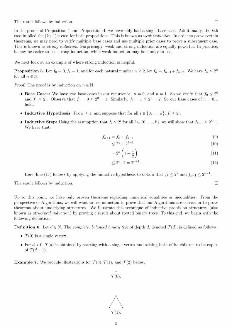
Definition 6. Let d ∈ N. The complete, balanced binary tree of depth d, denoted T (d), is defined as follows.

T (0) is a single vertex.

For d > 0, T (d) is obtained by starting with a single vertex and setting both of its children to be copiesof T (d− 1).

Example 7. We provide illustrations for T (0), T (1), and T (2) below.

T (0).

T (1).

5

T (2).

Proposition 8. The tree T (d) has 2d − 1 non-leaf nodes.

Proof. The proof is by induction on d ∈ N, the depth of the tree.

Base Case: We consider the base case of d = 0. Note that T (0) consists precisely of a single vertex,which is a leaf node. So T (0) has 20 = 1 leaf node. Thus, T (0) has 0 = 20− 1 non-leaf nodes, as desired.

Inductive Hypothesis: Fix d ≥ 0, and suppose that T (d) has 2d − 1 non-leaf nodes.

Inductive Step: We will use the assumption that T (d) has 2d− 1 non-leaf nodes to show that T (d+1)has 2d+1 − 1 non-leaf nodes. By construction, T (d + 1) consists of a single root node v, where each ofv’s two children are copies of T (d). By the inductive hypothesis, both the left and right copies of T (d)have 2d − 1 non-leaf nodes. This accounts for 2(2d − 1) non-leaf nodes in T (d+ 1). Note that v is also anon-leaf node. So T (d+ 1) has:

2(2d − 1) + 1 = 2d+1 − 2 + 1

= 2d+1 − 1

non-leaf nodes, as desired.

The result follows by induction.

Remark 9. In the inductive step of Proposition 8, observe that we used the structure of T (d + 1) to obtainthe number of non-leaf nodes. Precisely, we used the fact that T (d+ 1) is constructed by taking a root nodev and setting each of its children to be copies of T (d). We then used the inductive hypothesis to obtain thenumber of non-leaf nodes in the copies of T (d). That is, we had to use the construction of T (d+ 1) to obtainthe initial count of 2(2d − 1) + 1 non-leaf nodes.

A common and significant mistake would be to simply use algebraic manipulations to show that 2(2d−1)+1 =2d+1 − 1, without first showing that T (d+ 1) has 2(2d − 1) + 1 non-leaf nodes.

1.1 Supplemental Reading

For more resources on proof by induction, we recommend Richard Hammack’s Book of Proof (Chapter 10)[Ham20, Ch. 10], as well as Joe Fields’ A Gentle Introduction to the Art of Mathematics (Chapter 5) [Fie15,Ch. 5].

6

2 Graph Traversals

In this section, we examine graph traversal algorithms. Intuitively, a graph traversal takes as input a specifiedsource vertex, which we call s, and attempts to visit the remaining vertices in the graph. As a graph mayhave cycles, we need to take care not to revisit nodes, so as to avoid looping indefinitely. To this end, wemark vertices as visited once they have been evaluated. A graph traversal then only examines the unvisitedneighbors of the current vertex being considered.

We begin with the depth-first and breadth-first traversal algorithms. The depth-first traversal algorithm hasa myriad of applications, such as finding connected components on a graph, testing whether a graph is pla-nar, topological sorting, and exploring mazes. We may discuss some of these applications, such as topologicalsorting, later in the course. Other applications, such as generating and solving mazes, appear in subsequentcourses such as Artificial Intelligence.

The breadth-first search algorithm similarly has a number of applications. For our purposes, the key applicationof the breadth-first traversal is that it correctly finds shortest paths in unweighted graphs. For weighted graphs,the breadth-first traversal fails. This motivates Dijkstra’s algorithm.

2.1 Depth-First Traversal

The Depth-First Traversal algorithm takes as input a graph G, together with a source vertex s ∈ V (G). Werecursively traverse the unvisited neighbors of s. Effectively, DFS places the edges of s on to a stack. It thenpops off the first edge sv and recursively examines the neighbor v. The algorithm terminates when there areno more unvisited neighbors of s. We include pseudo-code below.

Algorithm 1 Depth-First Traversal

1: procedure DFS(Graph G,Vertex s)2: s.visited← true

3: for each unvisited neighbor v of s do4: DFS(G, v)

Example 10. We consider an example of the Depth-First Traversal procedure on the following graph G.

s

B

C

D

E

F

Suppose we invoke DFS(G, s). For the purpose of this example, we examine the unvisited neighbors of thecurrent vertex. Note that one could alternatively choose to order the vertices in a different way, which wouldresult in visiting the vertices in a different order. We also use red nodes to denote visited vertices. Thealgorithm does the following.

1. We first set s.visited := true.

7

s

B

C

D

E

F

2. Both neighbors of s, B and C, are unvisited. So we recurse and visit B next, invoking DFS(G,B).

s

B

C

D

E

F

3. Now the two unvisited neighbors of B are C and D. We visit C next, as we are choosing to order theneighbors alphabetically. We invoke DFS(G,C).

s

B

C

D

E

F

4. The only unvisited neighbor of C is E, so we next invoke DFS(G,E).

s

B

C

D

E

F

5. The unvisited neighbors of E are D and F . We visit D next, as D comes before F alphabetically. Weinvoke DFS(G,D).

8

s

B

C

D

E

F

6. The only unvisited neighbor of D is F . So we invoke BFS(G,D).

s

B

C

D

E

F

7. Now F has no unvisited neighbors. So DFS(G,F ) returns control to the invoking call DFS(G,D).

8. Similarly, as D has no unvisited neighbors, DFS(G,D) returns control to the invoking call DFS(G,E).

9. Now E has no unvisited neighbors. So DFS(G,E) returns control to the invoking call DFS(G,C).

10. As C has no unvisited neighbors, DFS(G,C) returns control to the invoking call DFS(G,B).

11. Now B has no unvisited neighbors, so DFS(G,B) returns control to the invoking call DFS(G, s).

12. As s has no unvisited neighbors, DFS(G, s) returns control to the line where it was invoked.

Remark 11. Using a different ordering would have resulted in traversing the vertices in a different order. Weillustrate this with the next example.

Example 12. In Example 10, we considered the result of calling DFS(G, s) on the following graph G, wherethe unvisited neighbors were examined in alphabetical order. We choose to select neighbors arbitrarily; thatis, not according to a prescribed rule. This yields a different order in which the vertices are visited. There arealternative choices one may make, which will again yield different orderings in which the vertices are visited.

s

B

C

D

E

F

1. As before, we start by setting s.visited := true.

9

s

B

C

D

E

F

2. The unvisited neighbors of s are B and C. We choose to visit C next. We invoke DFS(G,C).

s

B

C

D

E

F

3. The unvisited neighbors of C are B and E. We choose to visit E next, invoking DFS(G,E).

s

B

C

D

E

F

4. The unvisited neighbors of E are D and F . We choose to visit D next, invoking DFS(G,D).

s

B

C

D

E

F

5. The unvisited neighbors of D are B and F . We choose to visit B next, invoking DFS(G,B).

s

B

C

D

E

F

10

6. Now B has no unvisited neighbors, so DFS(G,B) returns control to DFS(G,D).

7. The only unvisited neighbor of D is F . So we invoke DFS(G,F ).

s

B

C

D

E

F

8. Now F has no unvisited neighbors, so DFS(G,F ) returns control to DFS(G,E).

9. As E has no unvisited neighbors, DFS(G,E) returns control to DFS(G,C).

10. Now C has no unvisited neighbors, so DFS(G,C) returns control to DFS(G, s).

11. Finally, DFS(G, s) returns control to the line where it was invoked.

11

2.2 Breadth-First Traversal

The Breadth-First Traversal algorithm works similarly to the Depth-First Traversal, except that the Breadth-First Traversal examines all of the unvisited neighbors of the current vertex before examning vertices furtheraway. In order to accomplish this, we place the neighbors of the current vertex in a queue and processsubsequent vertices based on the ordering enforced by the queue.

Algorithm 2 Breadth-First Traversal

1: procedure BFS(Graph G,Vertex s)2: s.visited← true

3: Queue Q← [s]4: while Q = [] do5: current← Q.poll()6: for each unvisited neighbor v of current do7: v.visited← true

8: Q.push(v)

Example 13. We consider an example of the Depth-First Traversal procedure on the following graph G. Asin Example 10, we examine the neighbors of the current vertex in alphabetical order.

s

B

C

D

E

F

We invoke BFS(G, s).

1. We set s.visited := true, then push s into the queue Q. So Q = [s].

s

B

C

D

E

F

2. We set current := Q.poll(). So current = s.

3. We now set the neighbors of s as visited and then push them into Q. So B.visited := true, C.visited :=true, and Q = [B,C].

s

B

C

D

E

F

12

4. We now set current := Q.poll(). So current = B.

5. We now mark the unvisited neighbors of B as visited and push them into the queue. SoD.visited := true,and Q = [C,D].

s

B

C

D

E

F

6. We now set current := Q.poll(). So current = C.

7. We now mark the unvisited neighbors of C as visited and push them into the queue. So E.visited := true,and Q = [D,E].

s

B

C

D

E

F

8. We now set current := Q.poll(). So current = D.

9. We now mark the unvisited neighbors of D as visited and push them into the queue. So F.visited := true,and Q = [E,F ].

s

B

C

D

E

F

10. We now set current := Q.poll(). So current = E. Now E has no unvisited neighbors, so we do not addany vertices to the queue. So Q = [F ].

11. We now set current := Q.poll(). So current = F . Now F has no unvisited neighbors, so we do not addany vertices to the queue. Now Q = []. As Q = [], the algorithm terminates.

Remark 14. Just as with the Depth-First Traversal, we need not examine the neighbors of the current vertexalphabetically.

13

2.3 Shortest-Path Problem: Unweighted Graphs

A problem of key interest in computer science is finding shortest paths between two vertices in a graph. Weconsider this problem for undirected, unweighted graphs. We note that in an unweighted graph, the length ofa path is the number of edges.

Example 15. As an example, we consider the graph below.

s

B

C

D

E

F

Consider the following paths.

The path D − E − F has length 2, as there are two edges. Note that D − E − F is not a shortest pathfrom D to F , as the path D − F has length 1.

In general, shortest paths are not unique. Observe that s − B − D − F and s − C − E − F are bothshortest paths from s to F .

Definition 16 (Unweighted Shortest Path Problem). The Unweighted Shortest Path problem is defined asfollows.

Instance: We take as input an undirected, unweighted graph G(V,E), together with prescribed verticess, t ∈ V (G).

Solution: The length of a shortest path from s to t.

It turns out that the Breadth-First Traversal algorithm can solve this problem. In fact, it does much more.Fix a starting vertex s in our graph G. Applying BFS(G, s) allows us to construct a tree T rooted at s, withthe property that for any vertex v ∈ V (G), the s to v path in T is a shortest s to v path in G. We call suchtrees single-source shortest path trees, or SSPTs. I will often refer to these as shortest-path trees.

We may modify the Breadth-First Traversal algorithm to construct a SSPT in the following manner. Supposewe are currently examining the vertex u. As we examine u’s unvisited neighbor v, we add the edge u, v toour tree. We consider the following example.

Example 17. Recall Example 13, where we added the unvisited neighbors to the queue in alphabetical order.We again use the same graph G, below.

s

B

C

D

E

F

We seek to find the shortest s to v path, for every vertex v ∈ V (G).

1. We begin by marking s as visited and pushing s into the queue. So Q = [s], and our intermediary treeis as follows:

14

s

2. We next poll s from Q. We now mark both neighbors of s, B and C, as visited and place them into thequeue. So B.visited = true, C.visited = true, and Q = [B,C]. We now add the edges s,B and s, Cto the tree. So our intermediary tree is as follows.

s

B

C

3. We next poll B from Q. We now mark the unvisited neighbor of B, which is D, as visited and place Dinto the queue. So D.visited = true, and Q = [C,D]. We now add the edge B,D to the tree. So ourintermediary tree is as follows.

s

B

C

D

4. We next poll C from Q. We now mark the unvisited neighbor of C, which is E, as visited and place Einto the queue. So E.visited = true, and Q = [D,E]. We now add the edge C,E to the tree. So ourintermediary tree is as follows.

s

B

C

D

E

5. We next poll D from Q. We now mark the unvisited neighbor of D, which is F , as visited and place Finto the queue. So F.visited = true, and Q = [E,F ]. We now add the edge E,F to the tree. So ourintermediary tree is as follows.

15

s

B

C

D

E

F

6. Note that the remaining elements of Q = [E,F ] have no unvisited neighbors. So we poll E, then poll F .Now as Q = [], the algorithm terminates. Our SSPT is:

s

B

C

D

E

F

We leave it to the reader to verify that for each vertex v, the s to v path in the tree above is a shortests to v path in our original graph G.

Remark 18. Recall that a tree on n vertices has n− 1 edges. So once we have placed five edges into the treefor Example 17, we may terminate the algorithm rather than processing the rest of the queue.

Remark 19. In Step 2 of Example 17, we placed B into the queue before C. Had we instead processed Cfirst, we would have obtained the following SSPT.

s

B

C

D

E

F

We record the fact that the Breadth-First Traversal solves the Unweighted Shotest Path problem with thefollowing theorem.

Theorem 20. Let G be an unweighted, undirected graph. Fix a vertex s ∈ V (G), and fix an ordering1 ≺ inwhich we place vertices into the queue when running the Breadth-First Traversal algorithm. Let T be the treeobtained by running BFS(G, s), using the ordering ≺. Then T is a single-source shortest path tree, with rootnode s.

Remark 21. While every tree produced by the Breadth-First Traveral algorithm is a SSPT, the converse isnot true. That is, there are SSPTs which cannot be obtained by BFS. We leave it to the reader to constructan example.

1For instance, we may place the neighbors of a given vertex v into the queue in alphabetical order, as in previous examples.However, different orderings may give rise to different SSPTs, as we saw with Remark 19.

16

2.4 Shortest-Path Problem: Weighted Graphs and Dijkstra’s Algorithm

In this section, we consider the Weighted Shortest Path Problem. We begin by introducing the notion of aweighted graph.

Definition 22. A weighted graph G(V,E,w) is a graph, together with a weight function w : E → R. That is,we label each edge with a real number. For a path P , the weight of P is the sum of the edge weights in P .

Example 23. Consider the following graph. Here, the number on the edge is the weight. So w(B,C) = 5,and w(A,D) = 1. The weight of the path P := A−B − E is:

w(P ) = w(A,B) + w(A,E) = 6 + 2 = 8.

A B C

D E

6

1

5

22

5

1

We now define the Weighted Shortest Path problem.

Definition 24. The Weighted Shortest Path problem defines as follows.

Instance: Let G(V,E,w) be a weighted graph, and let u, v ∈ V (G).

Solution: Determine the length of a minimum-weight (shortest) path from u to v.

Remark 25. For this section, we restrict attention to when the weights are all non-negative. That is, forany edge x, y, we have that w(x, y) ≥ 0. Dijkstra’s algorithm may fail to correctly solve the WeightedShortest Path problem in the presence of negative edge weights. In general, when we allow for both positiveand negative edge weights, the Weighted Shortest Path problem is quite hard. There is compelling evidencethat there is no efficient (polynomial-time) algorithm to solve the general Weighted Shortest Path problem.2

A natural first step is to consider whether the Breadth-First Traversal algorithm correctly solves the WeightedShortest Path problem. It turns out that the Breadth-First Traversal fails to do so; we leave constructing anexample as a homework exercise. Instead, we modify the Breadth-First Traversal to use a priority queue,rather than a queue, to provide the next vertex to consider. Precisely, we start by marking each vertex asun-processed. A vertex is only marked as processed once it is polled from the priority queue. Suppose wepolled the vertex x from the priority queue. We examine each un-processed neighbor y of x. If the path froms→ x→ y is shorter than the current known distance from s to y, then we do the following:

(a) We set dist(s, y) := dist(s, x)+w(x, y). If y is already in the priority queue, then we update its positionin line. Otherwise, we push y on to the priority queue.

(b) We set y.predecessor := x. By storing the predecessors, we may recover our desired shortest paths.

Note that by construction, no processed vertex can be pushed back on to the priority queue. This ensures thatthe algorithm terminates. Furthermore, as each vertex stores its predecessor, Dijkstra’s algorithm effectivelyconstructs a SSPT.

The algorithm we just described is known as Dijkstra’s algorithm. We include the formal algorithm below.

2Precisely, the Weighted Shortest Path problem is NP-hard. Algorithms that solve the general Weighted Shortest Path problemcan be adapted to detect the presence of Hamiltonian paths in unweighted graphs by setting each edge to have weight −1. SoHamiltonian paths correspond precisely to paths of weight −(n − 1) (where n is the number of vertices), and no path can haveweight smaller than −n. Determining whether a graph has a Hamiltonian path is a well-known NP-hard problem. We will formalizethese notions of hardness later in the course, during our discussions of the P vs. NP problem.

17

Algorithm 3 Dijkstra’s Algorithm

Require: The graph G is connected and has no negative-weight edges.1: procedure Dijkstra(WeightedGraph G(V,E,w),Vertex s)2: PriorityQueue Q← []3: for each v ∈ V (G) do4: v.dist←∞5: v.predecessor = NULL

6: Q.push(v)

7: s.dist← 08: Q.updatePosition(s)

9: while Q = [] do10: current← Q.poll()11: current.processed = true

12: for each unprocessed neighbor y of current do

13: if current.dist + w(current, y) < y.dist then14: y.dist← current.dist + w(current, y)15: y.predecessor← current16: Q.updatePosition(y)

return G

2.4.1 Dijkstra’s Algorithm: Example 1

We now consider an example.

Example 26. Consider the graph G below. Suppose we invoke Dijkstra(G,A).

A B C

D E

6

1

5

22

5

1

We do the following. We will mark processed vertices in red and use thick edges to denote predecessors.

1. We set the distance attributes for all vertices other than A to ∞. The distance attribute of A is set to 0,and then we push A into the priority queue Q. So Q = [(A, 0)], and the graph with the distance markersis pictured below.

A

0

B

∞

C

∞

D

∞

E

∞

6

1

5

22

5

1

2. We now poll A from the priority queue and set A.processed = true. Now the unprocessed neighbors ofA are B and D. Observe that:

18

w(A,B) = 6 <∞. So we set:

B.dist = 6,

B.predecessor = A,

and then push B into the priority queue.

Similarly, w(A,D) = 1 <∞. So we set:

D.dist = 1,

D.predecessor = A,

and then push D into the priority queue.

So the priority queue is Q = [(D, 1), (B, 6)]. The updated graph is below.

A

0

B

6

C

∞

D

1

E

∞

6

1

5

22

5

1

3. We now poll D from the priority queue and mark D as processed. The unprocessed neighbors of D areB and E. Observe that:

dist(A,D) + w(D,B) = 1 + 2 < 6. So we set:

B.dist = 3, and

B.predecessor = D.

As B is in the priority queue, we update its position. [Note: As B is the only element in thepriority queue, the update position call will simply return control without making changes.]

As dist(A,D) + w(D,E) = 1 + 1 <∞, we set:

E.dist = 2,

E.predecessor = D,

and then push E into the priority queue.

So the priority queue is Q = [(E, 2), (B, 3)]. The updated graph is below.

A

0

B

3

C

∞

D

1

E

2

6

1

5

22

5

1

19

4. We now poll E from the priority queue and mark E as processed. The two unprocessed neighbors of Eare B and C. Observe that:

dist(A,E) + w(E,B) = 2 + 2 < 3. So we make no further changes to B.

As dist(A,E) + w(E,C) = 2 + 5 <∞, we set:

C.dist = 7,

C.predecessor = E,

and then push C into the priority queue. So

So the priority queue is Q = [(B, 3), (C, 7)]. The updated graph is below.

A

0

B

3

C

7

D

1

E

2

6

1

5

22

5

1

5. We poll B from the priority queue and mark B as processed. The only unprocessed neighbor of B is C.As:

dist(A,B) + w(B,C) = 3 + 5 < 7,

we make no changes to C. So the priority queue is Q = [(C, 7)], and the updated graph is below.

A

0

B

3

C

7

D

1

E

2

6

1

5

22

5

1

6. We poll C from the priority queue and mark C as visited. As C has no unprocessed neighbors and Q isempty, the algorithm terminates. The final graph is below.

A

0

B

3

C

7

D

1

E

2

6

1

5

22

5

1

20

So Dijkstra’s algorithm found the following shortest paths from A.

A to B: The shortest path found was A−D −B, which has weight 3.

A to C: The shortest path found was A−D − E − C, which has weight 7.

A to D: The shortest path found was A−D, which has weight 1.

A to E: The shortest path found was A−D − E, which has weight 2.

21

2.4.2 Dijkstra’s Algorithm: Example 2

Example 27. We consider a second example on the graph below. Suppose we invoke Dijkstra(G,A).

A BC

D E

F

1

3

4

4

2

3

1

8

1. We set the distance attributes for all vertices other than A to ∞. The distance attribute of A is set to 0,and then we push A into the priority queue Q. So Q = [(A, 0)], and the graph with the distance markersis pictured below.

A

0

B

∞

C

∞

D

∞

E

∞

F

∞

1

3

4

4

2

3

1

8

2. We now poll A from the priority queue and set A.processed = true. Now the unprocessed neighbors ofA are C and F . Observe that:

w(A,C) = 1 <∞. So we set:

C.dist = 1,

C.predecessor = A,

and then push C into the priority queue.

Similarly, w(A,F) = 3 <∞. So we set:

F.dist = 3,

F.predecessor = A,

and then push F into the priority queue.

So the priority queue is Q = [(C, 1), (F, 3)]. The updated graph is below.

22

A

0

B

∞

C

1

D

∞

E

∞

F

3

1

3

4

4

2

3

1

8

3. We now poll C from the priority queue and set C.processed = true. Now the unprocessed neighbors ofC are B, D, and F . Observe that:

dist(A,C) + w(C,B) = 1 + 4 <∞. So we set:

B.dist = 5,

B.predecessor = C,

and then push B into the priority queue.

Similarly, dist(A,C) + w(C,D) = 1 + 3 <∞. So we set:

D.dist = 4,

D.predecessor = C,

and then push D into the priority queue.

We have that dist(A,C) + w(C,F) = 1 + 1 < 3. So we set:

F.dist = 2,

F.predecessor = C,

and then update F ’s position in the priority queue.

So the priority queue is Q = [(F, 2), (D, 4), (B, 5)]. The updated graph is below.

A

0

B

5

C

1

D

4

E

∞

F

2

1

3

4

4

2

3

1

8

23

4. We now poll F from the priority queue and set F.processed = true. Now the unprocessed neighbor of Fis B. Observe that:

dist(A,F ) + w(B,F) = 2 + 2 < 5. So we set:

B.dist = 4,

B.predecessor = F,

and we update B’s position in the priority queue. [Note: You may choose to either move B aheadof D or keep it after D.]

So the priority queue is Q = [(D, 4), (B, 4)]. The updated graph is below.

A

0

B

4

C

1

D

4

E

∞

F

2

1

3

4

4

2

3

1

8

5. We now poll D from the priority queue and set D.processed = true. Now the unprocessed neighbor ofD is E. Observe that:

dist(A,D) + w(D,E) = 4 + 8 <∞. So we set:

E.dist = 12,

E.predecessor = D,

and we push E into the priority queue.

So the priority queue is Q = [(B, 4), (E, 12)]. The updated graph is below.

A

0

B

4

C

1

D

4

E

12

F

2

1

3

4

4

2

3

1

8

24

6. We now poll B from the priority queue and set B.processed = true. Now the unprocessed neighbor ofB is E. Observe that:

dist(A,B) + w(B,E) = 4 + 4 < 12. So we set:

E.dist = 8,

E.predecessor = B,

and we update E’s position in the priority queue.

So the priority queue is Q = [(E, 12)]. The updated graph is below.

A

0

B

4

C

1

D

4

E

8

F

2

1

3

4

4

2

3

1

8

7. We poll E from the priority queue. As E has no unprocessed neighbors and Q is empty, the algorithmterminates. The final graph is below.

A

0

B

4

C

1

D

4

E

8

F

2

1

3

4

4

2

3

1

8

So Dijkstra’s algorithm found the following shortest paths from A.

A to B: The shortest path found was A− C − F −B, which has weight 4.

A to C: The shortest path found was A− C, which has weight 1.

25

A to D: The shortest path found was A− C −D, which has weight 4.

A to E: The shortest path found was A− C − F −B − E, which has weight 8.

A to F : The shortest path found was A− C − F , which has a weight of 2.

26

2.5 Dijkstra’s Algorithm: Proof of Correctness

In this section, we establish the correctness of Dijkstra’s algorithm, as well as analyze its runtime complexity.We begin by showing that Dijkstra’s algorithm terminates.

Proposition 28. Let G(V,E,w) be a finite, simple, connected, and weighted graph with no negative weightedges. Let s ∈ V (G) be the selected source vertex. Dijkstra’s algorithm terminates.

Proof. Suppose to the contrary that Dijkstra’s algorithm does not terminate. So the priority queue Q is neverempty. As we poll one vertex from Q at each iteration, it follows that at least one vertex is pushed on to thequeue at each iteration. We note that vertices that have been removed from Q are marked as processed andnever placed back into Q. It follows that G must be infinite, a contradiction.

We now seek to show that Dijkstra’s algorithm correctly computes a single-source shortest path tree. To thisend, we first introduce the following lemma, which establishes that the restriction of a shortest u to v path toany pair of vertices x, y along this path yields a shortest x to y path.

Lemma 29. Let G be a connected, undirected graph, and let u, v ∈ V (G) be vertices. Let P be a shortestpath from u to v. If x, y are vertices in P , then the sub-graph Pxy of P with endpoints x and y is a shortest xto y path in P .

Proof. Suppose to the contrary that Pxy is not a shortest path from x to y. Let Q be a shortest x to y pathin G. We have two cases.

Case 1: Suppose that the only vertices Q shares with P are x and y, then we may shorten P by replacingPxy. That is, we use the path P ′ := Pux · Q · Pyv. By construction, w(P ′) < w(P ), contradicting theassumption that P is a shortest path from u to v.

Case 2: Suppose that Q contains a vertex z ∈ Pyv. Then we may shorten P by using the pathP ′ := Pux ·Qxz · Pzv. By construction, w(P ′) < w(P ), contradicting the assumption that P is a shortestpath from u to v.

Case 3: Suppose that Q contains a vertex z ∈ Pxv. We apply the same argument as in Case 2, reversingthe roles of x and y.

The result follows.

We now show that Dijkstra’s algorithm correctly computes the shortest s to v path, for every vertex v.

Theorem 30. Let G(V,E,w) be a finite, simple, connected, and weighted graph such that all edge weightsare non-negative. Suppose that we run Dijkstra’s algorithm on G, using the source vertex s. Let dist(s, v)denote the distance from s to v computed by Dijkstra’s algorithm, and let d∗(s, v) be the length of a shortestpath from s to v. After Dijkstra’s algorithm terminates, we have for all v ∈ V (G), that dist(s, v) = d∗(s, v).

Proof. The proof is by induction on k, the number of vertices polled from the priority queue.

Base Case: When k = 0, we have polled no vertices from the priority queue. By construction dist(s, s) =d∗(s, s) = 0, as desired.

Inductive Hypothesis: Fix ℓ ≥ 0. Suppose that for each of the ℓ vertices s = v1, . . . , vℓ polled fromthe priority queue that dist(s, vi) = d∗(s, vi) for all i ∈ 1, . . . , ℓ.

Inductive Step: Let vℓ+1 be the (ℓ+1)st vertex polled from the priority queue. Suppose to the contrarythat the dist(s, vℓ+1) > d∗(s, vℓ+1). We note that at the point where vℓ+1 was polled from the priorityqueue, that dist(s, vℓ+1) is realized via a path containing only vertices from v1, . . . , vℓ. So for anyshortest path P from s to vℓ+1, there exists an unprocessed vertex w in P . Fix such a shortest s to vℓ+1

path P , and let w be the unprocessed vertex in P that is closest to s. By Lemma 29, the sub-path of Pwith endpoints s and w, which we denote Psw, is a shortest s to w path. So d∗(s, w) ≤ d∗(s, vℓ+1).

Now as w is the first unprocessed vertex in Psw, the predecessor of w in Psw is vi for some i ∈ v1, . . . , vℓ.Now Dijkstra’s algorithm would have examined the vi, w edge after polling vi from the priority queue;at which point, w would have been placed into the priority queue. Thus, the distance computed byDijkstra’s algorithm dist(s, w) < dist(s, vℓ+1). It follows that w would have been polled before vℓ+1,contradicting the fact that w was unprocessed. It follows that dist(s, vℓ+1) = d∗(s, vℓ+1).

27

We now turn towards analyzing the runtime complexity of Dijkstra’s algorithm. We first need to understandthe complexity of implementing the priority queue. Suppose we implement the priority queue using a standardbinary heap. Recall that the binary heap operations have the following runtime complexities:

Insertion: O(log(n)).

Removing the first element from the priority queue: O(log(n)).

Updating an element’s position: O(log(n)).

Searching: O(n)

We note that the loop at line 3 of Dijkstra’s Algorithm (see, 3) examines each vertex once, taking O(log(n))steps at each iteration. Here, the O(log(n)) complexity comes from pushing each vertex into the priority queue.So the complexity of lines 2-8 is O(|V | log(|V |)), where |V | is the number of vertices in the graph.

Now lines 9-16 examine each edge of G exactly once. At line 10, we poll a single vertex from the priorityqueue. As G is connected, we poll each vertex from the queue exactly once. As polling takes time O(log(n)),this adds complexity O(|V | · log(|V |)). Now when we evaluate each edge, we at most update the position of avertex in the priority queue. This accounts for time complexity O(|E| · log(|V |)), where |E| is the number ofedges in the graph. Thus, the time complexity of Dijkstra’s algorithm is O(|V | log(|V |) + |E| log(|V |)), whenusing a binary heap as our priority queue. We record this with the following theorem.

Theorem 31. The time complexity of Dijkstra’s algorithm is O(|V | log(|V |) + |E| log(|V |)), when using abinary heap as our priority queue.

28

2.6 Supplemental Reading

For more on the Breadth and Depth First Traversals, we defer to Errickson [Err, Chapters 4-6], CLRS [CLRS09,Chapter 22], Kleinberg & Tardos [KT05, Chapter 2], and OpenDSA [Tea21, Chapter 19.3] (use the Canvasversion of All Current OpenDSA Content).

For supplemental reading on Dijkstra’s algorithm, we defer to Errickson [Err, Chapter 8], CLRS [CLRS09,Chapter 24], Kleinberg & Tardos [KT05, Chapter 3.3], and OpenDSA [Tea21, Chapter 19.5] (use the Canvasversion of All Current OpenDSA Content).

29

3 Greedy Algorithm Principles

3.1 Exchange Arguments

In this section, we explore a key proof technique used in establishing the correctness of greedy algorithms;namely, the notion of an exchange argument. The key idea is to start with a solution (multi)set S and showthat we may swap out or exchange elements of S in such a way that improves the solution. Understandingwhich elements to exchange often provides key insights into designing effective greedy algorithms. Such provableobservations imply the correctness of our greedy algorithms.

Example 32. Recall the Making Change problem, where we have an infinite supply of pennies (worth 1 cent),nickels (worth 5 cents), dimes (worth 10 cents), and quarters (worth 25 cents). We take as input an integern ≥ 0. The goal is to make change for n using the fewest number of coins possible. The greedy algorithmchooses as many quarters as possible, followed by as many dimes as possible, then as many nickels as possible.Finally, the greedy algorithm uses pennies to finish making change.

Why is the greedy algorithm correct? Why does it select dimes before nickels? Exchange arguments allow usto answer this question. Consider the following lemma.

Lemma 33. Let n ∈ N be the amount for which we wish to make change. In an optimal solution, we have atmost one nickel.

Proof. Let S be the multiset of coins used to make change for n. Suppose that S contains k > 1 nickels. Thekey idea is that we may exchange each pair of nickels for a single dime. We formalize this as follows.

By the Division Algorithm, we may write k = 2j+r, where j ∈ N and r ∈ 0, 1. As k > 1, we have that j ≥ 1.So we exchange 2j nickels for j dimes to obtain a new solution set S′. Observe that: |S′| = |S| − j < |S|. Aswe may construct a solution using fewer coins, it follows that any optimal solution uses at most one nickel.

While we will not go through a full proof of correctness for the greedy algorithm to make change, similarlemmas regarding dimes and pennies serve as key steps in establishing the correctness of this algorithm. Infact, Lemma 33 provides the key insight that we should select dimes before nickels; as otherwise, we may needto swap out the nickels for fewer dimes.

In the next section, we will examine an application of the exchange argument to reason about the IntervalScheduling problem.

3.1.1 Supplemental Reading

We refer to Errickson [Err, Chapter 4] and Kleinberg & Tardos [KT05, Chapter 3.2] for supplemental readingon exchange arguments.

30

3.2 Interval Scheduling

In this section, we consider the Interval Scheduling problem. Intuitively, we have a single classroom. The goalis to assign the maximum number of courses to the classroom, such that no two classes are scheduled for ourroom at the same time. We now turn to formalizing the Interval Scheduling problme. Here, we think of intervalsas line segments on the real line. We specify each interval by a pair si and fi, where si < fi. An interval withstarting point si and ending point si is the set:

[si, fi] = x ∈ R : si ≤ x ≤ fi.

As an example, [0, 1] is the set of real numbers between 0 and 1, including the endpoints 0 and 1. Intuitively,the Interval Scheduling problem takes as input I, a set of intervals. The goal is to find the maximum numberof intervals we can select, such that no two intervals overlap.

Definition 34. The Interval Scheduling problem is defined as follows.

Instance: Let I = [s1, f1], . . . , [sk, fk] be our set of intervals.

Solution: A set S ⊆ I such that no two intervals in S overlap, where |S| is as large as possible.

We consider some examples.

Example 35. Let I = [0, 1], [1, 2], [2, 3]. Note that [0, 1] and [1, 2] overlap in the point 1. Similarly, [1, 2]and [2, 3] overlap in the point 2. So any maximum sized set of pairwise disjoint intervals can only contain atmost two intervals. Our unique maximum solution set is S = [0, 1], [2, 3]. As [1, 2] overlaps with both [0, 1]and [2, 3], we cannot add [1, 2] to S.In order to help visualize the problem, the intervals are pictured below.

c

ba

Example 36. Let I be the set of intervals pictured below. Observe that the maximum set of pairwise non-overlapping intervals is S = b, c, d.

a

bc

de

We now turn towards designing a greedy algorithm for the Interval Scheduling problem. The most naturalapproach is to place the intervals into a priority queue, polling the intervals one at a time. We store a set Sof intervals. As we poll an interval [si, fi] from the priority queue, we place it in S precisely if [si, fi] does notoverlap with any of the intervals stored in S. The key issue is to determine how order the intervals within thepriority queue. There are several natural orderings, including:

(a) Sorting the intervals from earliest start time to latest start time.

(b) Sorting the intervals by their length. Note that the length of an interval [s, f ] is f − s.

(c) Sorting the intervals from earliest end time to latest end time.

The following lemma (Lemma 37) provides the key insight that sorting the intervals from earliest end time tolatest end time yields a greedy algorithm that solves the Interval Scheduling problem. Note that Lemma 37 doesnot suggest that all such optimal solutions are of this form, or that there is a unique optimal solution. Rather,Lemma 37 only provides that there exists an optimal solution which is obtained by selecting the intervals fromearliest end time to latest end time. The proof of Lemma 37 is adapted from [Mou17].

31

Lemma 37. Let I be a set of intervals, and let S = [s1, f1], . . . , [sm, fm] be a set of pairwise non-overlappingintervals. Without loss of generality, suppose that f1 < f2 < . . . < fm. Suppose that there is an interval[s, f ] ∈ I and an index i ∈ 1, . . . ,m such:

fi−1 < s < f < fi.

So [s, f ] overlaps with at most one interval: [s, f ]. Then:

S′ = [s1, f1], . . . , [si−1, fi−1], [s, f ], [si+1, fi+1], . . . , [sm, fm]

is a set of pairwise non-overlapping intervals of size |S|.

Proof. As fi−1 < s, we have that [s, f ] does not overlap with [s1, f1], . . . , [si−1, fi−1]. Similarly, as f < fi < si+1,it follows that [s, f ] does not overlap with [si+1, fi+1], . . . , [sm, fm]. So S′ is a set of pairwise non-overlappingintervals. The result follows.

In light of Lemma 37, we propose the following greedy algorithm for the Interval Scheduling problem. We usethe ordering ⪯end, where [si, fi] ⪯end [sj , fj ] precisely if fi ≤ fj .

Algorithm 4 Interval Scheduling

1: procedure GreedyIntervalScheduling(IntervalSet I,Ordering ⪯)2: PriorityQueue Q← []3: Q.addAll(I,⪯) ▷ Sort the elements of I according to the ordering ⪯4: S ← ∅5: while Q = [] do6: I ← Q.poll()7: if I does not overlap with any interval in S then8: S.add(I)

Example 38. We apply our algorithm to the set of intervals I = a, b, c, d, e, where the intervals are picturedbelow.

a

bc

de

The algorithm proceeds as follows.

1. We start by placing the intervals into the priority queue Q, ordered from earliest finish time to latestfinish time. So Q = [b, a, c, d, e]. Our solution set S is initialized to S := ∅.

2. We first poll b from the priority queue. As S = ∅, b does not overlap with any interval in S. So we setS := S ∪ b = b.

3. We next poll a from the priority queue. As a overlaps with b, we discard a.

4. We next poll c from the priority queue. As c does not overlap with b, we set S := S ∪ c. So S = b, c.

5. We next poll d from the priority queue. As d does not overlap with either b or c, we set S := S ∪ d.So S = b, c, d.

6. We finally poll e from the priority queue. As e overlaps with at least one interval in S, we discard e.

7. The algorithm returns the solution set S = b, c, d.

We now turn to proving that our algorithm for Interval Scheduling (Algorithm 4) yields an optimal solution.There are two things we have to show.

32

(a) We first show that Algorithm 4 yields a set of pairwise non-overlapping intervals. Note that this holdsregardless of the ordering we choose to use.

(b) Now suppose that we order the intervals from earliest end time to latest end time. We show that forany interval set I, Algorithm 4 returns a maximum-sized set of pairwise non-overlapping intervals whenusing the ordering ⪯end.

Lemma 39. For any ordering ⪯, Algorithm 4 yields a set of pairwise non-overlapping intervals.

Proof. Algorithm 4 only adds an interval [s, f ] to the solution set S if [s, f ] does not overlap with any intervalalready in S. The result follows.

We now show that when ordering the intervals from earliest end time to latest end time, that Algorithm 4yields a maximum-sized set of pairwise non-overlapping intervals. This effectively follows by applying Lemma37 inductively. Our proof of Theorem 40 is adapted from [Mou16a].

Theorem 40. Recall the ordering ⪯end, where [si, fi] ⪯end [sj , fj ] precisely if fi ≤ fj . Algorithm 4, using thisordering ⪯end, returns a maximum sized set of pairwise disjoint intervals.

Proof. Let Si denote the solution set stored at the start of iteration i. We first show by induction on i thatthere exists an maximum-sized set of pairwise disjoint intervals Oi containing Si.

Base Case: We first consider the case when i = 0. So before any element is polled from the priorityqueue, S0 = ∅. As every set contains the emptyset, we have that some optimal solution O0 contains S0.

Inductive Hypothesis: Fix k ≥ 0, and let Sk be the solution set at the start of iteration k. Supposethat there exists an maximum-sized solution set Ok that contains Sk.

Inductive Step: Let Sk+1 be the solution set at the start of iteration k + 1, and let I be the intervalpolled at iteration k. We have two cases.

– Case 1: If I overlaps with an element of Sk, then I was not added to k. In this case, Sk+1 = Sk.By the inductive hypothesis, there exists a maximum-sized solution set Ok that contains Sk. So Ok

contains Sk+1 as well.

– Case 2: Suppose that I does not overlap with any interval in Sk. So Sk+1 = Sk ∪ I. By theinductive hypothesis, there exists a maximum-sized solution set Ok that contains Sk. As Ok is amaximum-sized solution set for the Interval Scheduling problem and Sk+1 is a set of pairwise non-overlapping intervals such that |Sk+1| = |Sk|+ 1, it follows that |Ok| ≥ |Sk+1|.

Suppose that the elements of Ok are ordered from earliest finish time to latest finish time. Let Jbe the (k + 1)st interval in Ok under this ordering. If I = J , then Ok contains Sk+1, and we aredone. Suppose instead that I = J . As Sk is contained in both Sk+1 and Ok, we have that the firstk intervals (under the ordering of intervals from earliest finish time to latest finish time) of Sk+1

and Ok agree. Now we write I = [s, f ] and J = [x, y]. As Algorithm 4 selects intervals based on theearliest end time, it follows that Algorithm 4 considered I before J . So f ≤ y. Thus, by Lemma37, Ok+1 := (Ok \ J) ∪ I is also a maximum-sized solution. Additionally, Ok+1 contains Sk+1,as desired.

So by induction, we have that the solution set S∗ returned by the algorithm is contained in some optimalsolution O.

We now claim that S∗ is an optimal solution. Suppose to the contrary that S∗ ⊊ O. Then there exists aninterval I in O that is not contained in S∗. As I does not overlap with any interval in O, we have that I doesnot overlap with any interval of S∗. So the greedy algorithm would have placed I in S∗, contradicting theassumption that S∗ ⊊ O. Thus, S∗ is indeed an optimal solution, as desired.

3.2.1 Supplemental Reading

The course notes by Mount [Mou17] and Moutadid [Mou16a] serve as good references for the Interval Schedulingproblem. Errickson [Err, Chapter 4.2], CLRS [CLRS09, Chapter 16], and Kleinberg & Tardos [KT05, Chapter3.1] also serve as standard references on the Interval Scheduling Problem.

33

3.3 Example Where the Greedy Algorithm Yields Sub-Optimal Solutions

The greedy technique is quite powerful. However, not all problems are amenable to greedy solutions. In thissection, we examine one such problem: finding maximum-sized matchings in arbitrary graphs. We begin byintroducing the notion of a matching.

Definition 41. Let G(V,E) be a graph. A matching M is a set of edges such that no two edges inM sharea common vertex. That is, if i, j, u, v ∈ M, then i = u, i = v and j = u, j = v.

We now consider some examples.

Example 42. Consider the cycle graph C6 pictured below.

1 2

3

45

6

There are several matchings on C6. We consider some of them below.

(a) First,M = ∅ is a matching of C6. As there are no edges inM, the condition that every pair of distinctedges fromM are disjoint is vacuously satisfied.

(b) Let i, j be an arbitrary edge of C6. ThenM = i, j is a matching of C6. As there is only one edgeinM, no two distinct edges ofM share any endpoints.

(c) Consider the set S = 1, 2, 2, 3. As 1, 2 and 2, 3 share a common endpoint (namely, the vertex2), the set S is not a matching.

(d) Consider the set M = 1, 2, 3, 4. As 1, 2 and 3, 4 do not share any endpoints in common, Mis a matching.

(e) The set M = 1, 2, 3, 4, 5, 6 is a matching, as no two edges share any endpoints in common.Observe that any remaining edge of C6 shares an endpoint with exactly two edges ofM. For instance,2, 3 shares the vertex 2 in common with 1, 2 and the vertex 3 in common with 3, 4. As 2, 3shares an endpoint in common with at least one edge ofM, the setM∪2, 3 is not a matching. Bysimilar argument,M∪ 4, 5 andM∪ 1, 6 are also not matchings of C6.

Example 43. Consider the following graph G, pictured below.

1 2 3

4

5

6

We consider some examples of matchings on G.

34

(a) LetM1 = 2, 3. Observe that every other edge of G shares an endpoint with 2, 3. Therefore,M1

does not sit inside a larger matching.

(b) LetM2 = 1, 2, 3, 5. Observe that every other edge of G shares an endpoint with either 1, 2 or3, 5. Therefore,M2 does not sit inside a larger matching.

We note thatM1 andM2 are both maximal, in the sense that neitherM1 norM2 sit inside a larger matching.However, M1 has a single edge, while M2 has two edges. Now the maximum number of edges a matchingof our graph G can have is 2. Therefore, M2 is a maximum-sized matching, while M1 is maximal but notmaximum-sized.

We now formalize the notions of maximal and maximum matchings.

Definition 44. Let G(V,E) be a graph, and letM be a matching of G. We say thatM is maximal if there isno other matchingM′ such thatM ⊊M′. That is,M is maximal if no other matching of G strictly containsM.

We say that M is a maximum-cardinality matching if M has the maximum number of possible edges. Thematching number ν(G) is the size of a maximum-cardinality matching of G.

We now consider the Maximum-Cardinality Matching problem.

Definition 45. The Maximum-Cardinality Matching problem is defined as follows.

Instance: Let G(V,E) be a graph.

Solution: A matchingM of G that has size |M| = ν(G).

We consider the following greedy algorithm, in an attempt to solve the Maximum-Cardinality Matching problem.

Algorithm 5 GreedyMatching

1: procedure GreedyMatching(Graph G)2: Queue Q← []3: Q.addAll(E(G))4: M← ∅5: while Q = [] do6: e← Q.poll()7: if e does not share an endpoint with any edge inM then8: M.add(e)

Algorithm 5 clearly produces a matching, as it only adds an edge e toM if e does not share an endpoint withany edge already in M. Furthermore, as the algorithm examines every edge, the matching M is maximal.However, the matching returned depends on the order in which the edges are added to the queue. We consideran example.

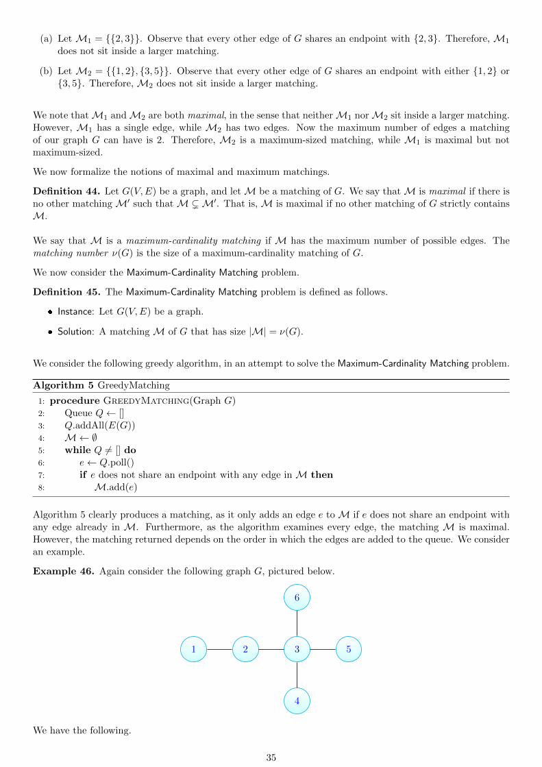
Example 46. Again consider the following graph G, pictured below.

1 2 3

4

5

6

We have the following.

35

Suppose that Algorithm 5 adds the edges to the queue in the following order:

Q = [2, 3, 3, 6, 3, 4, 3, 5, 1, 2].

The first edge considered is 2, 3. As all other edges of G share an endpoint with 2, 3, we have thatthe matching constructed by Algorithm 5 isM = 2, 3.

Suppose that Algorithm 5 adds the edges to the queue in the following order:

Q = [1, 2, 2, 3, 3, 6, 3, 4, 3, 5].

The first edge considered is 1, 2, which is added to our matching. Now as 2, 3 shares an endpointwith 1, 2, the algorithm discards 2, 3. We next consider 3, 6, which we add to the matching. Theremaining edges in Q, 3, 4 and 3, 5, each share an endpoint with either 1, 2 or 3, 6. So thematching constructed by Algorithm 5 isM = 1, 2, 3, 6.

So Algorithm 5 is not guaranteed to return a maximum-cardinality matching.

36

4 Spanning Trees

In this section, we introduce the Minimum Spanning Tree problem. We begin with a motivating example. Sup-pose a town experiences a snowstorm. It is imperative that that the residents are able to travel between anytwo destinations. However, given the volume of snow, plowing all of the roads will take time. Longer roads willalso take more time to clear. Therefore, we seek to find the shortest roads to clear, such that clearing thosespecific roads will allow for travel between any two destinations.

We may formalize this problem using the language of graph theory. Here, the destinations are the vertices ofour graph. There is an edge u, v in our graph precisely if there is a road connected u and v. The weightof the edge w(u, v) is the length of the road. Determining which roads to plow is equivalent to finding aminimum-weight spanning tree of our graph. We formalize this problem as follows.

Definition 47. The Minimum Spanning Tree problem is defined as follows.

Instance: An undirected, connected, and weighted graph G(V,E,w), where w : E(G)→ R is the functionassigning a real-valued weight to each edge.

Solution: A spanning tree T of G such that w(T ) is minimized. Recall that:

w(T ) :=∑

e∈E(T )

w(e).

4.1 Preliminaries: Trees

In order to design efficient algorithms to construct minimum-weight spanning trees, we seek to answer twomain questions:

(a) How many edges belong to a spanning tree?

(b) Which edges of the input graph should we include in the spanning tree?

Understanding the theory of trees allows us to answer these questions. We begin by recalling the definitionsof both a tree and a cut edge.

Definition 48. A tree is a connected, acyclic graph.

Definition 49. Let G(V,E) be a graph. An edge e ∈ E(G) is said to be a cut edge if G− e is not connected.

There are three key properties of interest when discussing trees: connectivity, acyclicity, and the number ofedges. We will show that if a graph has any two properties drawn from (i) being connected, (ii) having nocycles, and (iii) having n − 1 edges (where n is the number of vertices); then the graph necessarily has allthree properties. As a result, we note that any spanning tree has n− 1 vertices. Additionally, these propertiessuggest that we retain edges from the input graph that connect the graph, but do not create cycles.

Theorem 50. Let T (V,E) be a graph on n vertices. The following are equivalent.

(a) T is a tree. (That is, T is a connected, acyclic graph.)

(b) T is acyclic and has n− 1 edges.

(c) T is connected and has n− 1 edges.

Proof. We have the following.

(a) =⇒ (b) and (c): As a tree is connected and acyclic, it suffices to show that T has n− 1 edges. Wedo so by induction on n, the number of vertices. When n = 1, T consists of a single vertex and has noedges. Now fix k ≥ 1 and suppose that any tree on at most k vertices has k − 1 edges. Let T be a treeon k + 1 vertices. As k + 1 ≥ 2, T has a leaf vertex, which we call v. Note that T − v is a tree with kvertices. So by the IH, T − v has k − 1 edges. As v is a leaf in T , deg(v) = 1. So T − v has one feweredge than T . Thus, T has k edges. The result follows by induction.

37

(b) =⇒ (a) and (c): Let T be an acyclic graph with n − 1 edges. Let X1, . . . , Xk be the connectedcomponents of T . As T is acyclic, X1, . . . , Xk are trees. So by the proof that (a) =⇒ (b) and (c), wehave that Xi has |Xi| − 1 edges. As each vertex appears in exactly one component of T , we have that:

k∑i=1

(|Xi| − 1) = n− k.

As we have n− 1 edges by assumption, k = 1. So T is connected.

(c) =⇒ (a) and (b): Suppose T is a connected graph on n− 1 edges. We first recall that if C is a cyclein T and e is an edge on C, then T − e remains connected. So while T has a cycle, we remove an edge onsaid cycle. As T is finite, this procedure will terminate. We label the updated tree as T ′. Let k denotethe number of edges removed from T to obtain T ′. We note that T ′ is connected (as none of the edgesremoved were cut edges) and acyclic. So T ′ is a tree, with the same vertex set as T . By the (a) =⇒(b) and (c) paragraph, we note that T ′ has n − 1 edges. By assumption, T also has n − 1 edges, whichimplies that no edges were removed from T to obtain T ′. So T = T ′. Thus, T is acyclic.

Theorem 50 suggests a couple of algorithms for constructing spanning trees.

The first approach is to first sort the edges of the graph from lowest weight to highest weight. We thenconstruct a tree by adding edges one at a time, so long as they do not create a cycle. This algorithm isknown as Kruskal’s Algorithm.

The second approach is to first sort the edges of the graph from highest weight to lowest weight. We thenconstruct a tree by removing edges from the graph one at a time, so long as removing a given edge doesnot disconnect the remaining graph. This second algorithm is known as the Reverse-Delete algorithm.We will not pursue the Reverse-Delete algorithm further in this class.

While both algorithms will construct spanning trees, it is less clear that these algorithms (or even, otheralgorithms) return minimum-weight spanning trees. As all spanning trees on n vertices have n − 1 edges, itseems plausible to use an exchange argument that exchanges one edge for exactly one other edge, in order toprove that our algorithms return minimum-weight spanning trees. Theorem 50 does not provide sufficientlyprecise insights as to the exchange. To this end, we introduce additional characterizations of trees. The proofsof these characterizations provide insights on how to exchange edges. We will apply these proof techniques inthe next section to begin reasoning as to which edges are safe to include in a minimum-weight spanning tree.

Theorem 51. Let T (V,E) be a graph on n vertices. The following are equivalent.

(a) T is a tree.

(b) T is connected; and for every edge e ∈ E(T ), T −e is not connected. [That is, T is minimally connected.]

(c) For every pair of vertices u, v ∈ V (T ), there exists a unique path from u to v in T .

(d) T contains no cycles; and for any vertices u, v ∈ V (T ) such that u, v ∈ E(T ), adding the edge u, vcreates a cycle in T . [That is, T is maximally acyclic.]

Proof. We have the following.

(a) =⇒ (b): Let T be a tree, and let e = u, v ∈ E(T ). Suppose to the contrary that T−e is connected.So there exists a u− v path P in T , where P = u, v. So P ∪ u, v is a cycle, which implies that T hasa cycle. This contradicts the assumption that T has no cycles. So T − e is not connected.

(b) =⇒ (c): The proof is by contrapositive. Suppose there exist vertices u, v ∈ V (T ), such that thereexist two u − v paths in T . Label these paths P1, P2, where we provide P1 and P2 as sequences ofvertices: P1 = (x1, . . . , xk) and P2 = (y1, . . . , yj). As P1 = P2, there exist subpaths P

′1 = (xi, . . . , xh) and

P ′2 = (yℓ, . . . , ym) and P ′

1 and P ′2 agree only on the endpoints. It follows that P ′

1 ∪ P ′2 is a cycle. So not

every edge of T is a cut edge.

38

(c) =⇒ (a): As there exists a unique u − v path in T for every pair of vertices u, v ∈ T , we have thatT is connected. From the proof in the (b) =⇒ (c) direction, it follows that T is acyclic (for if T hadmultiple u− v paths for some vertices u, v, then T would have a cycle). Thus, T is a tree.

(a) =⇒ (d): As T is a tree, T contains no cycles. Let u, v ∈ V (T ) be non-adjacent vertices. So u, vis not a u− v path in T . As T is connected, there exists a u− v path P = uv in T . So P ∪ u, v formsa cycle.

(d) =⇒ (a): As T contains no cycles, it remains to show that T is connected. Suppose to the contrarythat T is not connected. Let X1, X2 be two connected components of T . Let u ∈ V (X1) and v ∈ V (X2).So u, v is a cut edge of T ∪u, v, which implies that T ∪u, v does not contain a cycle, a contradiction.

Remark 52. Theorem 51 suggests two exchange arguments. The first natural approach is to add an edge tothe tree, which creates a cycle, and then removing another edge from said cycle. The second approach is toremove an edge, which disconnects the tree; we then seek to the removed edge with another edge that connectsthe two components. We will apply these exchange techniques in the subsequent sections.

39

4.2 Safe and Useless Edges

Theorem 50 and Theorem 51 suggest that we should retain edges in the graph that connect the graph withoutcreating cycles. We note that these theorems only deal with unweighted graphs. As we are interested in findingminimum-weight spanning trees on weighted graphs, we need to modify the techniques from Section 4.1 tohandle edge weights. To this end, we introduce the notions of safe and useless edges. We follow closely theexposition from Carlson & Davies [CD20].

The key approach we will use in designing algorithms to find minimum-weight spanning trees is to manage anintermediate spanning forest and add edges until our forest becomes a tree. We wish to add edges in such away that the resulting spanning tree has minimum weight. We begin with the notions of an induced subgraphand intermediate spanning forest.

Definition 53. Let G(V,E) be a graph, and let S ⊆ V (G) be a set of vertices. The graph induced by S isthe graph H, where (i) the vertex set of H is S, and (ii) u, v ∈ E(H) precisely if u, v ∈ E(G). That is, westart with the vertices of S and add all available edges from G where both endpoints are in S.

Example 54. Consider the following graph G.

A

B

C

D

E

F

Let S = A,B,C,D. The subgraph H induced by S is pictured below. Note that only the edges of G whereboth endpoints belong to S are included.

A

B

C

D

The following graph K pictured below is not an induced subgraph. Here, our vertex set is S = D,E, F.Note that both the edges D,F and E,F are in G, so these edges do not cause our graph not to be induced.However, the edge D,E is in G, but not in K. Therefore, the absence of the edge D,E from K is why Kis not an induced subgraph.

D

F

E

We now turn to formalizing the notion of an intermediate spanning forest.

40

Definition 55. A forest F is a collection of disjoint trees T1, . . . , Tk. We say that F is a spanning forest ofthe graph G(V,E) if every vertex of V (G) is contained in F . Note that as the trees of F are disjoint, eachvertex v ∈ V (G) will be contained in exactly one tree of F .

Now we say that F is an intermediate spanning forest if (i) F is a spanning forest, and (ii) each tree Tj is aminimum-weight spanning tree on the graph induced by V (Tj).

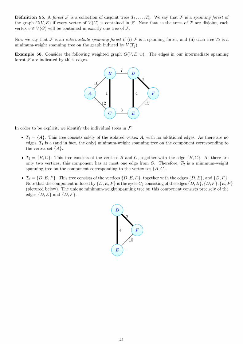
Example 56. Consider the following weighted graph G(V,E,w). The edges in our intermediate spanningforest F are indicated by thick edges.

A

B

C

D

E

F

10

12

1

7

3

4

2

15

In order to be explicit, we identify the individual trees in F :

T1 = A. This tree consists solely of the isolated vertex A, with no additional edges. As there are noedges, T1 is a (and in fact, the only) minimum-weight spanning tree on the component corresponding tothe vertex set A.

T2 = B,C. This tree consists of the vertices B and C, together with the edge B,C. As there areonly two vertices, this component has at most one edge from G. Therefore, T2 is a minimum-weightspanning tree on the component corresponding to the vertex set B,C.

T3 = D,E, F. This tree consists of the vertices D,E, F, together with the edges D,E, and D,F.Note that the component induced by D,E, F is the cycle C3 consisting of the edges D,E, D,F, E,F(pictured below). The unique minimum-weight spanning tree on this component consists precisely of theedges D,E and D,F.

D

F

E

4

2

15

41

We now consider a second example of an intermediate spanning forest.

Example 57. Consider the following weighted graph G(V,E,w). The edges in our intermediate spanningforest F are indicated by thick edges.

C

BA D

EH F

8

9

12 42

1

3

10

6

In order to be explicit, we identify the individual trees in F :

T1 = A,B. That is, this tree consists of the vertices A and B, together with the edge A,B. As thereis only one edge from G that can be included, T1 is a minimum-weight spanning tree on the componentinduced by the vertex set A,B.

T2 = H,F. That is, this tree consists of the vertices H and F , together with the edge H,F. By thesame reasoning as for T1, we have that T2 is a minimum-weight spanning tree on the component inducedby the verted set H,F.

T3 = C,D,E. That is, this tree consists of the vertices C,D,E, together with the edges C,Dand D,E. Note that the component induced by C,D,E is the cycle C3 consisting of the edgesC,D, D,E, C,E (pictured below). The unique minimum-weight spanning tree on this componentconsists precisely of the edges C,D and D,E.

C

D

E

4

1

3

We now introduce the notions of safe, light, and useless edges. Intuitively, a safe edge is an edge that canbe added to an intermediate spanning forest in such a way that we can still find a minimum-weight spanningtree of G. While precise, this definition of safe edge does not provide a useful way to efficiently identify whichedges to add. To this end, we have the notion of a light edge, which is a minimum-weight edge that crosses

42

a partition of the vertices. We will show later that light edges are safe. In particular, any light edge thatconnects two components in an intermediate spanning forest is safe. An edge is useless if it will create a cycle.As trees do not contain cycles, we do not include useless edges in our minimum-weight spanning trees. Weformalize these notions below.

Definition 58. Let G(V,E,w) be a weighted graph, and let F be an intermediate spanning forest of G. Lete = u, v be an edge of G such that e ∈ F .

(a) We say that e is safe with respect to F if F ∪ e is a subgraph of some minimum-weight spanning tree ofG.

(b) Let S ⊆ V (G) be a set of vertices such that every edge x, y in F has either x, y ∈ S or x, y ∈ V (G) \S.We say that e is a light edge e is a minimum weight edge with one endpoint in S and the other endpointin V (G) \ S.

(c) We say that e is useless with respect to F if both u and v lie on the same tree in F . Note that in thiscase, adding e to F creates a cycle.

(d) We say that e is undecided with respect to F if e is neither safe nor useless.

We now turn to showing that light edges are safe. The key proof technique is to start with a minimum-weightspanning tree T and exchange an edge that crosses the cut (S, V (G) \ S) (as in the definition of a light edge)for our light edge. As removing any edge of T disconnects T , we are effectively exchanging a cut edge of Tfor another cut edge. This exchange is very similar as in the proof of Theorem 51. Now as our light edge isa minimum-weight edge that crosses the cut, replacing an appropriate edge of T with our light edge does notincrease the weight of our modified tree. As T was assumed to be a minimum-weight spanning tree, we havethat our modified tree is also a minimum-weight spanning tree.

Theorem 59. Let G(V,E,w) be a weighted graph, and let A ⊆ E(G) be a subset of edges that belong to someminimum-weight spanning tree of G. Let S ⊆ V (G) such that every edge e = x, y ∈ A has either x, y ∈ S orx, y ∈ V (G) \ S (that is, no edge of S crosses the cut (S, V (G) \ S)). If u, v is an edge with one endpoint inS and the other endpoint in V (G) \ S, then u, v is a safe edge with respect to A.

Proof. Let T be a minimum-weight spanning tree of G that contains the edges of A. If T contains u, v, thenwe are done. So suppose that T does not contain u, v. As T is a spanning tree of G, there exists an edgee = a, b where one endpoint of e belongs to S, and the other endpoint belongs to V (G) \S (that is, e crossesthe cut (S, V (G) \S)). As T is a tree, every edge of T is a cut edge. So T \ e contains two components, T1 andT2. As u, v crosses the cut (S, V (G)\S), it follows (without loss of generality) that u ∈ V (T1) and v ∈ V (T2).So T ′ := (T \ e)∪ u, v is a spanning tree of G. As u, v is a light edge, w(u, v) ≤ w(e). So w(T ′) ≤ w(T ).As T is a minimum-weight spanning tree, it follows that w(T ′) = w(T ). So T ′ is a minimum-weight spanningtree. As A ∪ u, v ⊆ E(T ′), we have that u, v is safe, as desired.

Remark 60. As a corollary, we obtain that a light edge connecting two components in an intermediatespanning forest F is safe with respect to F . This allows us to easily identify safe edges. In addition, thiscorollary will be key in establishing the correctness of our minimum-weight spanning tree algorithms.

Corollary 61. Let G(V,E,w) be a weighted graph, and let F be an intermediary spanning forest. Fix a treeTi, and tet e ∈ E(G) be a light edge with exactly one endpoint in Ti. Then e is safe.

Proof. Let A be the set of edges in F . Let S = V (Ti). We apply Theorem 59 with the edge set A and thevertex set S to obtain that e is safe with respect to F .

We now apply Corollary 61 to help find safe edges.

Example 62. Consider again the following weighted graph G(V,E,w). The edges in our intermediate spanningforest F are indicated by thick edges.

43

A

B

C

D

E

F

10

12

1

7

3

4

2

15

We have the following.

A,B is the minimum-weight edge incident to A. Therefore, as A,B is a light edge with exactlyone endpoint belonging to A, we have by Corollary 61 that A,B is safe with respect to F .

C,E is the minimum-weight edge with exactly one endpoint in the component B,C (as well as theminimum-weight edge with exactly one endpoint in the component D,E, F). Therefore, we have byCorollary 61 that C,E is safe with respect to F .

While the edge A,C connects the components A and B,C, A,C is not a minimum-weight edgedoing so. Therefore, A,C is undecided with respect to F .

While the edge B,D connects the components B,C and D,E, F, B,D is not a minimum-weightedge doing so. Therefore, B,D is undecided with respect to F .

The edge E,F creates has both endpoints in the component D,E, F. So E,F is useless withrespect to F .

Example 63. We note that if the edge weights are not distinct, then there may be multiple safe edges for anintermediate spanning forest F . However, there are examples where we may only select one of the safe edges.Consider the cycle graph on four vertices, C4, pictured below. The edges of our intermediate spanning forestF are indicated by thick edges. While both B,C and C,D are safe with respect to F , only one of theseedges may be added to F . Adding both B,C and C,D would create a cycle.

A B

CD

1

1 1

1

44

4.3 Kruskal’s Algorithm

We briefly introduced Kruskal’s algorithm in Section 4.1. In this section, we will examine Kruskal’s algorithmin more detail. Recall that Kruskal’s algorithm places the edges of the input graph into a priority queue. Itthen polls the edges one at a time, adding the edge e currently being considered to the intermediate spanningforest precisely if e connects two disjoint components. As the edges are sorted from lowest weight to highestweight, it follows that e is added precisely if there exists a component T where e is a light edge with exactlyone endpoint in T . So by Corollary 61, e is added precisely if e is safe.

We formalize Kruskal’s algorithm below.

Algorithm 6 Kruskal’s Algorithm

1: procedure Kruskal(ConnectedWeightedGraph G(V,E,w))2: F ← (V (G), ∅) ▷ Initialize the Intermediate Spanning Forest to contain no edges.3: PriorityQueue Q← []4: Q.addAll(E(G))5: while F .numEdges() < |V (G)| − 1 do6: u, v ← Q.poll() ▷ Poll an edge and call the endpoints u and v7: if u and v are on different components of F then8: F .addEdge(u, v)

return F

Example 64. We now work through Kruskal’s algorithm on the following graph.

A

B

C

D

E

F

10

12

1

7

3

4

2

15

We proceed as follows.

1. We initialize the intermediate spanning forest F to be the empty graph (the graph on no edges). We alsoplace the edges of G into a priority queue, which we call Q. So:

Q = [(B,C, 1), (D,F, 2), (C,E, 3), (D,E, 4), (B,D, 7), (B,A, 10), (A,C, 12), (E,F, 15)].

Here, (B,C, 1) indicates the edge B,C has weight 1. The intermediate spanning forest F is picturedbelow.

A

B

C

D

E

F

2. We poll from Q, which returns the edge B,C. Note that w(B,C) = 1. As B and C are on differentcomponents of F , we add the edge B,C to F . So:

Q = [(D,F, 2), (C,E, 3), (D,E, 4), (B,D, 7), (B,A, 10), (A,C, 12), (E,F, 15)],

and the updated intermediate spanning forest F is pictured below.

45

A

B

C

D

E

F1

3. We poll from Q, which returns the edge D,F. Note that w(D,F) = 2. As B and C are on differentcomponents of F , we add the edge D,F to F . So:

Q = [(C,E, 3), (D,E, 4), (B,D, 7), (B,A, 10), (A,C, 12), (E,F, 15)],

and the updated intermediate spanning forest F is pictured below.

A

B

C

D

E

F1

2

4. We poll from Q, which returns the edge C,E. Note that w(C,E) = 3. As C and E are on differentcomponents of F , we add the edge C,E to F . So:

Q = [(D,E, 4), (B,D, 7), (B,A, 10), (A,C, 12), (E,F, 15)],

and the updated intermediate spanning forest F is pictured below.

A

B

C

D

E

F1

3

2

5. We poll from Q, which returns the edge D,E. Note that w(D,E) = 4. As D and E are on differentcomponents of F , we add the edge D,E to F . So:

Q = [(B,D, 7), (B,A, 10), (A,C, 12), (E,F, 15)],

and the updated intermediate spanning forest F is pictured below.

A

B

C

D

E

F1

3

4

2

46

6. We poll from Q, which returns the edge B,D. Note that w(B,D) = 7. As B and D are on the samecomponent of F , we do not add the edge B,D to F . So:

Q = [(B,A, 10), (A,C, 12), (E,F, 15)],

and the intermediate spanning forest F remains unchanged from the previous iteration.

7. We poll from Q, which returns the edge B,A. Note that w(B,A) = 10. As B and A are on differentcomponents of F , we add the edge B,A to F . So:

Q = [(A,C, 12), (E,F, 15)],

and the updated intermediate spanning forest F is pictured below.

A

B

C

D

E

F

10

1

3

4

2

As there are 6 vertices and F has 5 edges, Kruskal’s algorithm terminates and returns F , which is ourminimum-weight spanning tree.

Remark 65. Now that we have worked through an example of Kruskal’s algorithm, we wish to comment abit about the algorithm provided (Algorithm 6). On line 7 of Algorithm 6, there is an if statement checkingwhether two vertices belong to the same connected component. For the purposes of this class, we will notexamine the details associated with implementing this functionality. In practice, a Union-Find data structureis used to manage the intermediate spanning forest. We direct the reader to [CLRS09, Chapter 21] for detailsregarding the Union-Find data structure.

47

4.3.1 Kruskal’s Algorithm: Proof of Correctness

We now turn to proving that Kruskal’s algorithm returns a minimum-weight spanning tree. Precisely, we needto show the following.

(a) Kruskal’s algorithm terminates.

(b) Kruskal’s algorithm returns a spanning tree.

(c) The spanning tree that Kruskal’s algorithm returns is of minimum weight.

We begin by showing that Kruskal’s algorithm terminates.

Proposition 66. Let G(V,E,w) be a finite, connected, weighted graph. Kruskal’s algorithm terminates, whenapplied to G.

Proof. Kruskal’s algorithm examines each edge of G at most once. As G has finitely many edges, the algorithmterminates.

We next show that Kruskal’s algorithm returns a spanning tree. We do this in two parts. First, we showthat Kruskal’s algorithm returns a spanning forest. Next, we show that the final spanning forest is indeedconnected.

Proposition 67. LetG(V,E,w) be a finite, connected, weighted graph. Kruskal’s algorithm returns a spanningforest of G.

Proof. Kruskal’s algorithm begins with a spanning forest F of G that has no edges (see line 2 of Algorithm 6).At each iteration of Kruskal’s algorithm, at most one edge is added to F . As a necessary condition for a givenedge e to added to F , it must be the case that e does not create a cycle in F . So the graph that Kruskal’salgorithm returns indeed spans G and is acyclic. Thus, Kruskal’s algorithm returns a spanning forest of G, asdesired.

Proposition 67 provides that Kruskal’s algorithm indeed returns a spanning forest of G. We show that thisspanning forest is indeed a tree.

Proposition 68. LetG(V,E,w) be a finite, connected, weighted graph. Kruskal’s algorithm returns a spanningtree of G.

Proof. Let F be the spanning forest of G returned by Kruskal’s algorithm. Suppose to the contrary that F isnot connected (and therefore, not a tree). Let T1, . . . , Tk be the connected components of F . As G is connected,there exists an edge e = u, v of G that does not belong to F and has endpoints in two distinct components ofF . We take e = u, v to be such a minimum-weight edge. Let Ti be the component of F containing u, and letTj be the component of F containing v. As u and v belong to different components of F , adding e to F wouldnot create a cycle. In particular, as e is a minimum-weight edge with endpoints in different components of F ,Kruskal’s algorithm would have placed e into F (see lines 7-8 of Algorithm 6), contradicting the assumptionthat Kruskal’s algorithm returned a spanning forest that was not a tree. The result follows.

It remains to show that the spanning tree returned by Kruskal’s algorithm is a minimum-weight spanning tree.Recall that Corollary 61 states that if there is a component T such that the edge e is a light edge with exactlyone endpoint in T , then e is safe. We apply Corollary 61 and induction to show that Kruskal’s algorithmreturns a minimum-weight spanning tree.

Theorem 69. Let G(V,E,w) be a finite, connected, weighted graph. Kruskal’s algorithm returns a minimum-weight spanning tree of G.

Proof. Let F be the spanning forest that Kruskal’s algorithm maintains. We show by induction on the numberof iterations of Kruskal’s algorithm that F is an intermediate spanning forest. Note that if F has |V (G)| − 1edges, then F is a tree. So if F is an intermediate spanning forest with |V (G)| − 1 edges, then F is aminimum-weight spanning tree.

Base Case: Prior to the first iteration of Kruskal’s algorithm, F has no edges. So F is contained insome (and in fact, every) minimum-weight spanning tree of G. Thus, F is an intermediate spanningforest of G.

48

Inductive Hypothesis: Suppose that at the start of iteration m ≥ 0, F is an intermediate spanningforest of G.

Inductive Step: Let e = u, v be the edge polled from the priority queue at iteration m of Kruskal’salgorithm, and let F be the intermediate spanning forest at the start of iteration m. We note thatKruskal’s algorithm adds e to the intermediate spanning if and only if u and v belong to differentcomponents Ti and Tj of F . So suppose Kruskal’s algorithm adds e to F . As the priority queue storesedges in order from smallest weight to largest weight, it follows that (without loss of generality) e is aminimum-weight edge with exactly one endpoint in Ti. So e is a light edge with exactly one endpoint inTi. Thus, by Corollary 61, e is a safe edge and F ∪ e is an intermediate spanning forest.

The result follows by induction.

49

4.3.2 Kruskal’s Algorithm: Runtime Complexity

In this section, we turn to analyzing the runtime complexity of Kruskal’s algorithm. We begin by sortingthe edges of G from smallest weight to largest weight. Sorting the edges takes time O(|E| · log(|E|)), where|E| := |E(G)|. Now we note that there are at most

(|V |2

)edges in our input graph, where |V | := |V (G)|. So:

log(|E|) ≤ log

((|V |2

))≤ log(|V |2)= 2 log(|V |).

Thus, sorting the edges takes time O(|E| · log(|V |)). Next, we initialize a Union-Find data structure [CLRS09,Chapter 21] with each vertex of G as an isolated component. Here, we use the Union-Find to maintain theintermediate spanning forest. The Union-Find data structure has two keep operations, find and union, eachof which runs in time O(α(n)) (where n is the number of elements in the Union-Find). Here, α(n) is the inverseAckermann function, which grows much more slowly than O(log(n)). In the context of Kruskal’s algorithm, nis the number of vertices in the graph. So both the find and union operations run in time O(α(|V |)).

The find operation takes as input a vertex v and returns a distinguished vertex x that lies on the samecomponent as v. We note that if u and v belong to the same component, then find(u) = find(v).Conversely, if find(u) = find(v), then u and v lie on the same component.

The union operation combines two disjoint components into one component.

For each edge of G, Kruskal’s algorithm utilizes two find calls to determine if the endpoints of the edge belongto the same component. If the edges belong to different components, then Kruskal’s algorithm makes oneunion call to merge the components. So the total complexity of processing the edges after they are sorted isO(|E| · α(|V |)). Thus, the total runtime complexity of Kruskal’s algorithm is:

O(|E| · (log(V ) + α(|V |))) = O(|E| · log(|V |).

We record the complexity with the following theorem.

Theorem 70. Kruskal’s algorithm runs in time O(|E| · log(|V |).

50

4.4 Prim’s Algorithm

In this section, we examine a second technique to construct minimum-weight spanning trees; namely, Prim’salgorithm. We again start with the intermediate spanning forest F that contains all the vertices of our inputgraph G(V,E,w), but none of the edges. While Kruskal’s algorithm determines which edges to add to F byexamining the entire graph, Prim’s algorithm takes a more local perspective. We provide as input a specifiedsource vertex s ∈ V (G). Let T ∗ be the component of F that contains s. Prim’s algorithm examines the edgesof G that have exactly one endpoint in T ∗ and select a light edge e from these to add to F . As e has exactlyone endpoint in T ∗, e connects two distinct components of F . So by Corollary 61, e is a safe edge with respectto F . This is the key observation in establishing that Prim’s algorithm returns a minimum-weight spanning tree.

We now turn to formalizing Prim’s algorithm.

Algorithm 7 Prim’s Algorithm

1: procedure Prim(ConnectedWeightedGraph G(V,E,w),Vertex source)2: F ← (V (G), ∅) ▷ Initialize the Intermediate Spanning Forest to contain no edges.3: PriorityQueue Q← []

4: for each edge e ∈ E(G) do5: e.processed← false

6: for each edge e incident to source do7: Q.add(e)8: e.processed← true

9: while F .numEdges() < |V (G)| − 1 do10: u, v ← Q.poll() ▷ Poll an edge and call the endpoints u and v11: Tu ← F .componentContaining(u)12: Tv ← F .componentContaining(v)

13: if Tu = Tv then ▷ Check that u and v belong to different components14: F .addEdge(u, v)

15: if source ∈ Tu then ▷ If v was added to the component containing source16: for each unprocessed edge e incident to v do17: Q.add(e) ▷ Then add to Q each unprocessed edge incident to v

18: else ▷ If u was added to the component containing source19: for each unprocessed edge e incident to u do20: Q.add(e) ▷ Then add to Q each unprocessed edge incident to u

return F

We associate to each edge an attribute processed to indicate whether that edge has been placed into thepriority queue. This ensures that each edge is considered at most once, which helps ensure that the algorithmwill terminate.

Now at lines 6-8, we initialize the priority queue to contain only edges that are incident to the source vertex.This ensures that the first edge placed into the intermediate spanning forest is incident to the source vertex.Now by adding an edge to F , we introduce a new vertex v to the component containing our source vertex.Prim’s algorithm then adds to the prioritiy queue the edges incident to v, provided such edges have not alreadybeen polled from the queue. So the while loop at line 9 preserves the invariant that every edge in the priorityqueue has at least one endpoint in the component containing our source vertex.

Prim’s algorithm only adds an edge if it connects two components. Such an edge e is polled from the priorityqueue, and so (i) has an endpoint in the component containing the source vertex, and (ii) is a minimum-weightedge connecting two distinct components. Therefore, e is a safe edge.

51

4.4.1 Prim’s Algorithm: Example 1

We now work through an example of Prim’s algorithm.

Example 71. Consider the following graph G(V,E,w) pictured below. Suppose we select the source vertexA.

A

B

C

D

E

F

10

12

1

7

3

4

2

15

Prim’s algorithm proceeds as follows.

1. We initialize the intermediate spanning forest to contain all the vertices of G, but no edges. We theninitialize the priority queue to contain the edges incident to our source vertex A. So:

Q = [(A,B, 10), (A,C, 12)],

and our intermediate spanning forest F is pictured below.

A

B

C

D

E

F

2. We poll the edge A,B from the queue and mark A,B as processed. Note that w(A,B) = 10. AsA,B has exactly one endpoint on the component containing A (which is the isolated vertex A), we addA,B to F . We then push into the priority queue the unprocessed edges incident to B. So:

Q = [(B,C, 1), (B,D, 7), (A,C, 12)],

and the updated intermediate spanning forest F is pictured below.

A

B

C

D

E

F

10

3. We poll the edge B,C from the queue and mark B,C as processed. Note that w(B,C) = 1. AsB,C has exactly one endpoint on the component containing A (which is the isolated vertex A,B),we add B,C to F . We then push into the priority queue the unprocessed edges incident to C (providedsaid edges are not already in the priority queue). So:

Q = [(C,E, 3), (B,D, 7), (A,C, 12)],

and the updated intermediate spanning forest F is pictured below.

52

A

B

C

D

E

F

10

1

4. We poll the edge C,E from the queue and mark C,E as processed. Note that w(C,E) = 3. AsC,E has exactly one endpoint on the component containing A, we add C,E to F . We then pushinto the priority queue the unprocessed edges incident to E (provided said edges are not already in thepriority queue). So:

Q = [(E,D, 4), (B,D, 7), (A,C, 12), (E,F, 15)],

and the updated intermediate spanning forest F is pictured below.

A

B

C

D

E

F

10

1

3

5. We poll the edge E,D from the queue and mark E,D as processed. Note that w(E,D) = 4. AsE,D has exactly one endpoint on the component containing A, we add E,D to F . We then pushinto the priority queue the unprocessed edges incident to D (provided said edges are not already in thepriority queue). So:

Q = [(D,F, 2), (B,D, 7), (A,C, 12), (E,F, 15)],

and the updated intermediate spanning forest F is pictured below.

A

B

C

D

E

F

10

1

3

4

6. We poll the edge D,F from the queue and mark D,F as processed. Note that w(D,F) = 2. AsD,F has exactly one endpoint on the component containing A, we add D,F to F . We then pushinto the priority queue the unprocessed edges incident to D (provided said edges are not already in thepriority queue). So:

Q = [(B,D, 7), (A,C, 12), (E,F, 15)],

and the updated intermediate spanning forest F is pictured below.

53

A

B

C

D

E

F

10

1

3

4

2

7. As F has |V (G)| − 1 = 6 − 1 = 5 edges, the algorithm terminates and returns F , pictured in Step 6immediately above.

Remark 72. We note that the minimum-weight spanning tree constructed by Kruskal’s algorithm in Example64 is the same tree that Prim’s algorithm constructed in Example 71. For this input graph, the edge weightswere distinct. Therefore, the graph had only one minimum-weight spanning tree. In general, Prim’s algorithmand Kruskal’s do not construct the same minimum-weight spanning tree.

54

4.4.2 Prim’s Algorithm: Example 2

We consider a second example of Prim’s algorithm.

Example 73. Consider the following graph G(V,E,w). We execute Prim’s algorithm, using the source vertexD.

C

BA D

EH F

8

9

12 42

1

3

10

6

Prim’s algorithm proceeds as follows.

1. We initialize the intermediate spanning forest to contain all the vertices of G, but no edges. We theninitialize the priority queue to contain the edges incident to our source vertex A. So:

Q = [(D,E, 1), (D,C, 3)],

and our intermediate spanning forest F is pictured below.

C

BA D

EH F

2. We poll the edge D,E from the queue and mark D,E as processed. Note that w(C,E) = 1. AsD,E has exactly one endpoint on the component containing D, we add D,E to F . We then pushinto the priority queue the unprocessed edges incident to E (provided said edges are not already in thepriority queue). So:

Q = [(D,C, 3), (E,C, 4)],

and the updated intermediate spanning forest F is pictured below.

55

C

BA D

EH F

1

3. We poll the edge D,C from the queue and mark D,C as processed. Note that w(D,C) = 3. AsD,C has exactly one endpoint on the component containing D, we add D,C to F . We then pushinto the priority queue the unprocessed edges incident to C (provided said edges are not already in thepriority queue). So:

Q = [(E,C, 4), (C,A, 8), (C,B, 9), (C,F, 12)],

and the updated intermediate spanning forest F is pictured below.

C

BA D

EH F

1

3

4. We poll the edge E,C from the queue and mark E,C as processed. As both E and C belong to thecomponent containing D, we do not add E,C to F . The updated priority queue is below, and theintermediate spanning forest F does not change from the previous iteration.

Q = [(C,A, 8), (C,B, 9), (C,F, 12)].

5. We poll the edge C,A from the queue and mark C,A as processed. Note that w(C,A) = 8. AsC,A has exactly one endpoint on the component containing D, we add C,A to F . We then pushinto the priority queue the unprocessed edges incident to A (provided said edges are not already in thepriority queue). So:

Q = [(A,B, 2), (C,B, 9), (A,H, 10), (C,F, 12)],

and the updated intermediate spanning forest F is pictured below.

56

C

BA D

EH F

8

1

3

6. We poll the edge A,B from the queue and mark A,B as processed. Note that w(A,B) = 2. AsA,B has exactly one endpoint on the component containing D, we add A,B to F . We then pushinto the priority queue the unprocessed edges incident to B (provided said edges are not already in thepriority queue). So:

Q = [(C,B, 9), (A,H, 10), (C,F, 12)],

and the updated intermediate spanning forest F is pictured below.

C

BA D

EH F

8

2

1

3

7. We poll the edge C,B from the queue and mark C,B as processed. As both C and B belong to thecomponent containing D, we do not add C,B to F . The updated priority queue is below, and theintermediate spanning forest F does not change from the previous iteration.

Q = [(A,H, 10), (C,F, 12)],

8. We poll the edge A,H from the queue and mark A,H as processed. Note that w(A,H) = 10. AsA,H has exactly one endpoint on the component containing D, we add A,H to F . We then pushinto the priority queue the unprocessed edges incident to H (provided said edges are not already in thepriority queue). So:

Q = [(H,F, 6), (C,F, 12)],

and the updated intermediate spanning forest F is pictured below.

57

C

BA D

EH F

8

2

1

3

10

9. We poll the edge H,F from the queue and mark H,F as processed. Note that w(H,F) = 6. AsH,F has exactly one endpoint on the component containing D, we add A,H to F . We then pushinto the priority queue the unprocessed edges incident to H (provided said edges are not already in thepriority queue). So:

Q = [(C,F, 12)],

and the updated intermediate spanning forest F is pictured below.

C

BA D

EH F

8

2

1

3

10

6

As F has |V (G)| − 1 = 7 − 1 = 6 edges, the algorithm terminates and returns F , pictured in Step 8immediately above.

58

4.4.3 Algorithm 7 Correctly Implements Prim’s Algorithm

Prim’s algorithm works by, at a given iteration, adding a light edge with exactly one endpoint in the com-ponent containing the source vertex. We proposed an implementation of Prim’s algorithm with Algorithm 7.In this section, we show that Algorithm 7 adds at each iteration a light edge with exactly one endpoint inthe component containing the source vertex. That is, we show that Algorithm 7 correctly implements Prim’salgorithm. We are not showing in this section that Prim’s algorithm returns a minimum-weight spanning tree;those details will be covered in the next section.

We first show that Algorithm 7 only adds edges to the priority queue where at least one endpoint is containedin same component as the source vertex.

Lemma 74. Prior to the start of iteration i ≥ 0 of the while loop on line 9 of Algorithm 7, the priority queueQ only contains edges where at least one endpoint is in the same connected component as the source vertex.

Proof. The proof is by induction on the number of iterations of the while loop on line 9.

Base Case: Prior to the start of the while loop, the edges incident to the source vertex are placed inthe priority queue (see lines 6-7). So the priority queue contains edges where at exactly one endpoint isin the same connected component as the source vertex.

Inductive Hypothesis: Fix k ≥ 0. Suppose that prior to the start of iteration k of the while loop online 9, that the priority queue Q contains only edges where at least one endpoint of each edge belongs tothe same connected component as the source vertex.

Inductive Step: Let e = u, v be the edge polled at iteration k of the while loop. By the inductivehypothesis, at least one endpoint of e belongs to the same connected component as the source vertex.We have two cases.

– Case 1: Suppose both u and v belong to the same connected component as the source vertex. Inthis case, the condition of the if statement on line 13 is not satisfied. So e is not added to F and nonew edges are added to the priority queue Q. By the inductive hypothesis, Q contains only edgeswhere at least one endpoint of each edge belongs to the same connected component as the sourcevertex, which remains true prior to the start of iteration k + 1 of the while loop.

– Case 2: Suppose exactly one endpoint of e belongs to the same connected component as the sourcevertex. Let Tu and Tv be the components of F containing u and v respectively. As exactly oneendpoint of e belongs to the same connected component as the source vertex, we have that Tu = Tv.So the condition of the if statement on line 13 is satisfied. Thus, Algorithm 7 adds e to F . Now ifsource is on the same component as u (that is, source ∈ Tu), then the algorithm adds the unprocessededges incident to v to the priority queue (provided said edges are not already in the priority queue).By similar argument, if instead source ∈ Tv, then the algorithm adds the unprocessed edges incidentto u to the priority queue (provided said edges are not already in the priority queue). In eithercase, Q contains only edges where at least one endpoint of each edge belongs to the same connectedcomponent as the source vertex, which remains true prior to the start of iteration k+1 of the whileloop.

The result follows by induction.

Remark 75. In the proof of Lemma 74, we showed that Algorithm 7 adds the edge e being considered at thegiven iteration to F precisely if e has exactly one endpoint in the connected component containing the sourcevertex. As the edges are sorted in from smallest weight to largest weight, it follows that Algorithm 7 adds eto F precisely if e is a light edge that has exactly one endpoint in the connected component containing thesource vertex. This observation, together with Lemma 74 yields the following.

Theorem 76. Algorithm 7 correctly implements Prim’s algorithm.

59

4.4.4 Prim’s Algorithm: Proof of Correctness

In this section, we establish the correctness of Prim’s algorithm. That is, we show that Prim’s algorithmreturns a minimum-weight spanning tree. Just as with Kruskal’s algorithm, we need to show the following.

(a) Prim’s algorithm terminates.

(b) Prim’s algorithm returns a spanning tree.

(c) The tree that Prim’s algorithm returns is of minimum-weight.

We begin by showing that Prim’s algorithm terminates.

Proposition 77. Let G(V,E,w) be a connected, weighted graph. Prim’s algorithm terminates, when appliedto G.

Proof. Prim’s algorithm examines each edge of G at most once. As G has finitely many edges, the algorithmterminates.

We next show that Prim’s algorithm returns a spanning tree. We do this in two parts. First, we show thatPrim’s algorithm returns a spanning forest. Second, we show that the spanning forest is connected.

Proposition 78. Let G(V,E,w) be a connected, weighted graph. Prim’s algorithm returns a spanning forestof G.

Proof. Prim’s algorithm initializes a spanning forest F of G that has no edges (see line 2 of Algorithm 7).At each iteration of Prim’s algorithm, at most one edge is added to F . As a necessary condition for Prim’salgorithm to add a given edge e, it must be the case that the endpoints of e belong to different components ofF . Thus, if an edge e is added to F , then F ∪ e does not contain a cycle. So the graph that Prim’s algorithmreturns indeed spans G and is acyclic. Thus, Prim’s algorithm returns a spanning forest of G, as desired.

We now show that the spanning forest F that Prim’s algorithm returns is indeed a tree.

Proposition 79. Let G(V,E,w) be a connected, weighted graph. Prim’s algorithm returns a spanning treeof G.

Proof. Let F be the spanning forest of G that Prim’s algorithm returns. Suppose to the contrary that F isnot connected. Let Tsource be the component of F associated with the source vertex, and let T1, . . . , Tk bethe remaining components of F . As G is connected, there exists an edge e ∈ E(G) such that one endpointis in Tsource and the other endpoint belongs to Ti for some i ∈ 1, . . . , k. In particular, there exists an edgee of minimum weight edge with one endpoint in Tsource and the other endpoint in Ti for some i ∈ 1, . . . , k.However, Prim’s algorithm would have added e to F , contradicting the assumption that Tsource and Ti werenot connected. The result follows.

It remains to show that the tree returned by Prim’s algorithm is a minimum-weight spanning tree. Recall thatCorollary 61 states that if for a component T , e is a light edge with exactly one endpoint in T , then e is a safeedge with respect to the given intermediate spanning forest. We apply Corollary 61 and induction to showthat Prim’s algorithm returns a minimum-weight spanning tree.

Theorem 80. Let G(V,E,w) be a connected, weighted graph. Prim’s algorithm returns a minimum-weightspanning tree of G.

Proof. Let F be the spanning forest that Prim’s algorithm maintains. We show by induction on the number ofiterations of Prim’s algorithm that F is an intermediate spanning forest. Note that if F has |V (G)| − 1 edges,then F is a tree. So if F is an intermediate spanning forest with |V (G)|−1 edges, then F is a minimum-weightspanning tree.

Base Case: Prior to the start of the first iteration, F has no edges. So F is contained in some (and infact, every) minimum-weight spanning tree of G. Thus, F is an intermediate spanning forest of G.

Inductive Hypothesis: Suppose that at the start of iteration m ≥ 0, F is an intermediate spanningforest of G.

60

Inductive Step: Let e = u, v be the edge polled from the priority queue at iteration m of Prim’salgorithm, and let F be the intermediate spanning forest at the start of iteration m. We note that Prim’salgorithm adds e to F if and only if exactly one endpoint of e belongs to the same component as thesource vertex. By Lemma 74, at least one endpoint of e belongs to the same component as the sourcevertex. So we have two cases.

– Case 1: Suppose that both endpoints of e belong to the same component as the source vertex. Inthis case, e is not added to F . So no changes to F are made, and we retain F as our intermediatespanning forest at the start of iteration m+ 1.

– Case 2: Suppose that exactly one endpoint of e belongs to the same component as the sourcevertex. As the priority queue stores edges in order from smallest weight to largest weight, it followsthat e is a minimum-weight edge with exactly one endpoint in the component containing the sourcevertex. So by Corollary 61, e is a safe edge and F ∪ e is an intermediate spanning forest.

The result follows by induction.

61

4.4.5 Prim’s Algorithm: Runtime Complexity

We now turn to analyzing the runtime complexity of our implementation (Algorithm 7) of Prim’s algorithm.We make several assumptions. First, we assume that the graph is provided as an adjacency list. Second, weuse a standard binary heap to implement the priority queue. Both the insert and poll operations take timeO(log(m)), where m is the number of elements in the priority queue. Now the worst case complexity of thebinary heap’s lookup operation is O(m). We circumvent this by using a processed attribute for each edge,to indicate whether that edge was placed into the priority queue. Algorithm 7 does not place processed edgesback into the priority queue, which ensures that each edge is examined at most once. We stress that as thepriority queue is storing edges, m := |E|.

Now as with Kruskal’s algorithm, we use the Union-Find data structure [CLRS09, Chapter 21] to implementthe intermediate spanning forest. Recall that both the union and find operations take O(n · α(n)) time,where α(n) is the inverse Ackermann function, which grows more slowly than O(log(n)). We stress that asthe Union-Find data structure is storing vertices, that n := |V |.

With our assumptions in tow, we begin analyzing the runtime complexity of Algorithm 7. Note that in theworst case for a given edge e = u, v, we do the following:

Place e into the priority queue,

Remove e from the priority queue,

Perform two find calls on the Union-Find, using the endpoints u and v (see lines 11-12).

Perform a union operation if u and v belong to different components (see line 14).

Thus, for a given edge, the worst case runtime complexity is O(log(|E|) + α(|V |)). An edge e = u, v isexamined twice. The first time occurs when we examine the edges incident to u, and the second time is whenwe examine the edges incident to v. Note that we are using the adjacency list structure at lines 15-20, in thatwe can examine each edge incident to a given vertex without traversing through the entire vertex set (whichwould be necessary if we were using an adjacency matrix representation of hte graph). Thus, in the worst case,Algorithm 7 takes time:

O(2|E| · (log(|E|) + α(|V |))) = O(|E| · (log(|E|) + α(|V |))) (13)

= O(|E| · log(|E|)) (14)

= O(|E| · log(|V |)). (15)

Here, line (14) follows from the fact that α(|V |) ∈ O(log(|V |)) ⊆ O(log(|E|)). Line (15) follows from the factthat |E| ≤

(|V |2

); so log(|E|) ≤ 2 log(|V |) ∈ O(log(|V |)). Thus, we have the following.

Theorem 81. Prim’s algorithm has the worst case time complexity O(|E| · log(|V |)) when using an adjacencylist for the graph, a binary heap to support the priority queue, and a Union-Find data structure to implementthe intermediate spanning forest.

62

5 Network Flows

In this chapter, we examine the notion of flows on networks. Intuitively, network flows are used to modelsettings such as routing oil from drilling platforms to shore, sending packets of information over the internet,routing electricity throughout a city, and scheduling. Here, our networks are directed graphs. Each edge (u, v)of the directed graph has a capacity c(u, v), which is the amount of flow that can be pushed through the edgefrom u to v. Note that flow is directional. Intuitively, flow can only move in one direction, such as pushing oilthrough a pipe. It is not possible to push oil both forwards and backwards along the same pipe.

5.1 Framework

We first formalize the network flows framework.

Definition 82. Let G(V,E) be a connected, directed graph. A source vertex s is a vertex with in-degree 0;that is, s has no incoming edges. A sink vertex t is a vertex with out-degree 0; that is, t has no outgoing edges.

Remark 83. Informally, a source vertex is where flow originates, and a sink vertex is a destination point. Thegoal of the flow problem is to push as much flow as possible from the source vertices to the sink vertices.

Definition 84. A flow network N (G, c, S, T ) consists of a directed graph G(V,E), together with a set S ofsource vertices and a set T of sink vertices. We note that S and T are disjoint sets. N also has a capacityfunction c : V (G) × V (G) → [0,∞), such that if the ordered pair (u, v) ∈ V (G) × V (G) is not an edge, thenc(u, v) = 0. This condition ensures that we can only push flow along edges.

Remark 85. For undirected graphs, we denote edges as sets of the form u, v. Recall that a set is a collectionof distinct, unordered elements. For undirected graphs, it is not the case that there are designated startingpoints and ending points along edges. So u, v = v, u. In the case of directed graphs, each edge has a clearstarting and ending point. For this reason, we denote edges as ordered pairs. The edge (u, v) indicates thatu is the starting vertex and v is the ending vertex. Similarly, (v, u) has v as the starting point and u as theending vertex. So we note that (u, v) = (v, u).

Our goal is to push flow across a flow network. To this end, we first formalize the notion of flow.

Definition 86. Let N (G, c, S, T ) be a flow network. A flow is a function f : V (G)×V (G)→ [0,∞) satisfyingthe following.

For any ordered pair (u, v) ∈ V (G)× V (G), f(u, v) ≤ c(u, v). That is, we cannot push more flow acrossa given edge than the capacity permits. Similarly, if the pair (u, v) ∈ E(G), then we cannot push flowacross (u, v). That is, we can only push flow along edges.

We have a conservation of flow condition. For every vertex v that is neither a source vertex nor a sinkvertex, we have that the amount of flow coming into v is the amount of flow leaving v.∑

(u,v)∈E(G)

f(u, v) =∑

(v,w)∈E(G)

f(v, w).

The value of f , denoted val(f) or |f |, is the amount of flow that is moved from the source nodes to the sinknodes. By the conservation of flow condition, |f | is precisely the amount of flow leaving the source nodes.

We now turn to considering examples of flow networks and flows.

Example 87. Consider the following flow network N (G, c, S, T ). We indicate both the flow and the capacityof a given edge using the labeling convention flow/capacity. For instance:

The edge (s,B) has capacity 10, and there are 4 units of flow being pushed from s→ A.

The edge (B,D) has capacity 4, and there are 4 units of flow being pushed from A→ B.

The edge (D, t) has capacity 10, and there are 5 units of flow being pushed from D → t.

The edge (C,E) has capacity 9, and there is 1 unit of flow being pushed from C → E.

63

s

B

C

D

E

t

4/10

2/10

0/2

4/4

0/6

2/9

1/3

5/10

1/2

Additionally, observe that for each vertex v other than the source s and the sink t, the flow coming into v isequal to the flow leaving v. We check this for the vertices other than s and t.

Observe that there are 4 units of flow coming into vertex B via the edge (s,B). These 4 units of flowleave B along the edge (B,D).

Observe that there are 4 units of flow coming into D via the edge (B,D). These 4 units of flow leave Dalong the edge (D, t).

Observe that there are 2 units of flow coming into C via the edge (s, C). These 2 units of flow leave Calong the edge (C,E).

Observe that there are 2 units of flow coming into E via the edge (C,E). Precisely 1 unit leaves E alongthe edge (E,D), and the other 1 unit of flow leaves E along the edge (E, T ).

We now consider examples of configurations that fail to be valid flows.

Example 88. Consider the following flow network. The flow configuration below is invalid, as flow is notconserved at vertex B. Here, 4 units of flow enter B through the edge (s,B). However, only 3 units of flowleave B (see the edge (B,D)).

s

B

C

D

E

t

4/10

2/10

0/2

3/4

0/6

2/9

1/3

3/10

1/2

Example 89. Consider the following flow network. The flow configuration is invalid, as the edges (s,A) and(A, t) each have capacity 10, but there are 11 units of flow being pushed through each edge.

s A t11/10 11/10

64

5.2 Flow Augmenting Paths

The goal of the max-flow problem is to move as much flow as possible from the source nodes to the sink nodes.We formalize this as follows.

Definition 90. The Maximum Flow problem is defined as follows.

Instance: We take as input a flow network N (G, c, S, T ), with no flow along any directed edge.

Solution: A flow function f∗ : V (G) × V (G) → [0,∞) such that |f∗| (the amount of flow leaving thesource nodes) is maximized.

Algorithmically, our general approach is to find paths along which we can move positive flow from a source toa sink. We call such paths flow-augmenting. While we can always push flow in the forward direction along anedge, we can also re-route existing flow back along an edge. Precisely, let (u, v) be an edge, and let f(u, v) bethe current flow that is being pushed from u → v. We may push at most c(u, v) − f(u, v) additional units offlow from u → v. Atlernatively, we may push f(u, v) units of flow back from v → u. We then re-route thisflow at v.

Example 91. Consider the following flow network. We examine certain directed edges to determine theamount of flow that can be pushed in the forward and backwards directions.

Consider the edge (D,C). There is currently 1 unit of flow being pushed from D → C, and (D,C) has acapacity of 6 units of flow. So we can push up to an additional 5 units of flow from D → C. Alternatively,we can take up to the 1 unit of flow currently being routed from D → C and push that flow backwardsfrom C → D.

Consider the edge (B,C). We may push 2 units of flow from B → C. As there is no current flow beingpushed from B → C, we may not push flow backwards from C → B.

Consider the edge (B,D). There are currently 3 units of flow being pushed from B → D. We may pushat most 1 additional unit of flow from B → D. Alternatively, we can take up to the 3 units of flowcurrently being routed from D → C and push that flow back from D → B.

s

B

C

D

E

t

3/10

1/10

0/2

3/4

1/6

2/9

0/3

2/10

2/2

We now turn to examining flow-augmenting paths for the above flow network.

We have that s → B → D → t is a flow-augmenting path. While we can push 7 units of flow froms → B, we can only push 1 unit of flow from B → D. Thus, we can only push 1 unit of flow along thepath s→ B → D → t.

We have that s→ B → C → D → t is a flow-augmenting path. While we can push 7 units of flow froms → B, we can only push 2 units of flow from B → C. Now as there is 1 unit of flow coming in fromC → D, we may push that 1 unit of flow backwards from C → D. So only 1 of the 2 units of flow thatmake it to C end up at D. We then push that 1 unit of flow from D → t. So we may push 1 unit of flowalong the path s→ B → C → D.

We have that s→ C → E → D → t is a flow-augmenting path. While we can push 9 units of flow froms→ C, we can only push back 7 units of flow from C → E. Of those 7 units of flow, we may only push3 units from E → D, as (E,D) has a capacity of 3. Now we push 3 units of flow from D → t. So alongthe flow augmenting path s→ C → E → D → t, we may push at most 3 units of flow.

65

We have that s→ C → D → t is a flow-augmenting path. While we can push 9 units of flow from s→ C,we can only push 1 unit of flow from C → D. We may then push this 1 unit of flow from D → t. So wemay push 1 unit of flow along the path s→ C → D → t.

66

5.3 Ford-Fulkerson Algorithm

In this section, we introduce the Ford-Fulkerson algorithm to solve the Maximum Flow problem. The key ideabehind the Ford-Fulkerson procedure is to iteratively select a flow-augmenting path and then push as muchflow as possible along said path.

Algorithm 8 Ford-Fulkerson

1: procedure FordFulkerson(FlowNetwork N )2: while N has a flow-augmenting path do3: Let P be a flow-augmenting path of N4: Push as much flow as possible along P

Remark 92. Algorithm 8 does not specify how to select flow-augmenting paths in an optimal manner. Wewill not delve into these details in this class; rather, we defer them for an Advanced Algorithms course. Forthe purposes of this class, it suffices to select your favorite flow-augmenting path at a given iteration.

We now work through some examples of the Ford-Fulkerson algorithm.

5.3.1 Ford-Fulkerson: Example 1

The example we consider in this section is based on the lecture slides of Wayne [Way05]. Consider the followingflow network.

s

B

C

D

E

t

0/10

0/10

0/2

0/4

0/8

0/9

0/6

0/10

0/10

We proceed as follows.

1. There are several flow-augmenting paths we could select at the first iteration, including:

s→ B → D → t

s→ B → E → t

s→ B → E → D → t

s→ B → C → E → t

s→ C → E → t

s→ C → E → D → t.

We make the choice to select the flow-augmenting path s → B → E → t, though we stress that anyof the flow-augmenting paths could be selected at the initial round. Again, we made a choice to selects→ B → E → t, rather than following a prescribed rule.

We push the full 8 units of flow from s→ B → E → t. The updated flow network is below.

67

s

B

C

D

E

t

8/10

0/10

0/2

0/4

8/8

0/9

0/6

0/10

8/10

2. There are several flow-augmenting paths we could select at the second iteration, including:

s→ B → D → t

s→ B → C → E → t

s→ C → E → t

s→ C → E → D → t.

We make the choice to select the flow-augmenting path s → B → C → E → t. Again, we stressthat any of the above flow-augmented paths could be selected instead at this round. The selection ofs→ B → C → E → t was arbitrary, rather than due to following a prescribed rule.

We push the full 2 units of flow from s→ B → C → E → t. The updated flow network is below.

s

B

C

D

E

t

10/10

0/10

2/2

2/4

8/8

2/9

0/6

0/10

10/10

3. There are several flow-augmenting paths we could select at the third iteration, including:

s→ C → E → D → t

s→ C → E → B → D → t

s→ C → B → D → t.

We make the choice to select the flow-augmenting path s → C → E → D → t. Again, we stressthat any of the above flow-augmented paths could be selected instead at this round. The selection ofs→ C → E → D → t was arbitrary, rather than due to following a prescribed rule.

We push the full 6 units of flow from s→ C → E → D → t. The updated flow network is below.

68

s

B

C

D

E

t

10/10

6/10

2/2

0/4

8/8

8/9

6/6

6/10

10/10

4. There are two flow-augmenting paths we could select at the fourth iteration, including:

s→ C → B → D → t

s→ C → E → B → D → t.

We make the choice to select the flow-augmenting path s → C → B → D → t. Again, we stressthat any of the above flow-augmented paths could be selected instead at this round. The selection ofs→ C → B → D → t was arbitrary, rather than due to following a prescribed rule.

We push the full 2 units of flow from s→ C → B → D → t. The updated flow network is below.

s

B

C

D

E

t

10/10

8/10

0/2

2/4

8/8

8/9

6/6

8/10

10/10

5. There is one flow-augmenting path at the fifth iteration: s → C → E → B → D → t. We push the full1 unit of flow across this path. The updated and final flow network is below.

s

B

C

D

E

t

10/10

9/10

0/2

3/4

7/8

9/9

6/6

9/10

10/10

There are no more flow-augmenting paths, so the algorithm terminates. The total flow pushed froms→ t is 19 units of flow.

69

5.3.2 Ford-Fulkerson: Example 2

We consider the same flow network as in the previous example. Here, we select alternative flow-augmentingpaths to illustrate that there is choice in selecting said paths.

s

B

C

D

E

t

0/10

0/10

0/2

0/4

0/8

0/9

0/6

0/10

0/10

We proceed as follows.

1. There are several flow-augmenting paths we could select at the first iteration, including:

s→ B → D → t

s→ B → E → t

s→ B → E → D → t

s→ B → C → E → t

s→ C → E → t

s→ C → E → D → t.

We make the choice to select s → C → E → t. Again, our choice is arbitrary, and not according to aprescribed rule.

We push the full 9 units of flow from s→ C → E → t. The updated flow network is below.

s

B

C

D

E

t

0/10

9/10

0/2

0/4

0/8

9/9

0/6

0/10

9/10

2. There are several flow-augmenting paths we could select at the second iteration, including:

s→ B → D → t

s→ B → E → D → t

s→ B → E → t.

We make the choice to select s → B → D → t. Again, our choice is arbitrary, and not according to aprescribed rule.

We push the full 4 units of flow from s→ B → D → t. The updated flow network is below.

70

s

B

C

D

E

t

4/10

9/10

0/2

4/4

0/8

9/9

0/6

4/10

9/10

3. There are two available flow-augmenting paths at the third iteration: s → B → E → D → t ands → B → E → t. We select the path s → B → E → D → t and push the full 6 units of flow along thispath. The updated flow network is below.

s

B

C

D

E

t

10/10

9/10

0/2

4/4

6/8

9/9

6/6

10/10

9/10

There are no more flow-augmenting paths, so the algorithm terminates. Observe that 19 units of floware being pushed from s→ t.

71

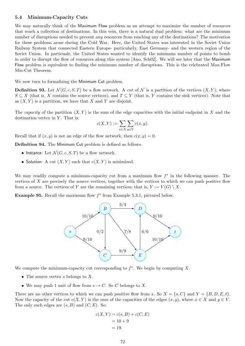
5.4 Minimum-Capacity Cuts

We may naturally think of the Maximum Flow problem as an attempt to maximize the number of resourcesthat reach a collection of destinations. In this vein, there is a natural dual problem: what are the minimumnumber of disruptions needed to prevent any resources from reaching any of the destinations? The motivationfor these problems arose during the Cold War. Here, the United States was interested in the Soviet UnionRailway System that connected Eastern Europe- particularly, East Germany- and the western region of theSoviet Union. In particualr, the United States wanted to identify the minimum number of points to bombin order to disrupt the flow of resources along this system [Ano, Sch02]. We will see later that the MaximumFlow problem is equivalent to finding the minimum number of disruptions. This is the celebrated Max-FlowMin-Cut Theorem.

We now turn to formalizing the Minimum Cut problem.

Definition 93. Let N (G, c, S, T ) be a flow network. A cut of N is a partition of the vertices (X,Y ), whereS ⊆ X (that is, X contains the source vertices), and T ⊆ Y (that is, Y contains the sink vertices). Note thatas (X,Y ) is a partition, we have that X and Y are disjoint.

The capacity of the partition (X,Y ) is the sum of the edge capacities with the initial endpoint in X and thedestination vertex in Y . That is:

c(X,Y ) :=∑x∈X

∑y∈Y

c(x, y).

Recall that if (x, y) is not an edge of the flow network, then c(x, y) = 0.

Definition 94. The Minimum Cut problem is defined as follows.

Instance: Let N (G, c, S, T ) be a flow network.

Solution: A cut (X,Y ) such that c(X,Y ) is minimized.

We may readily compute a minimum-capacity cut from a maximum flow f∗ in the following manner. Thevertices of X are precisely the source vertices, together with the vertices to which we can push positive flowfrom a source. The vertices of Y are the remaining vertices; that is, Y := V (G) \X.

Example 95. Recall the maximum flow f∗ from Example 5.3.1, pictured below.

s

B

C

D

E

t

10/10

9/10

0/2

3/4

7/8

9/9

6/6

9/10

10/10

We compute the minimum-capacity cut corresponding to f∗. We begin by computing X.

The source vertex s belongs to X.

We may push 1 unit of flow from s→ C. So C belongs to X.

There are no other vertices to which we can push positive flow from s. So X = s, C and Y = B,D,E, t.Now the capacity of the cut c(X,Y ) is the sum of the capacities of the edges (x, y), where x ∈ X and y ∈ Y .The only such edges are (s,B) and (C,E). So:

c(X,Y ) = c(s,B) + c(C,E)

= 10 + 9

= 19.

72

Observe that the capacity of the cut (X,Y ) is precisely the value |f∗| = 19, the amount of flow we can pushfrom s → t. This is no coincidence; in fact, this is the precise statement of the Max-Flow Min-Cut Theorem:the capacity of a minimum-capacity cut is the same as the value of a maximum flow. We will prove theMax-Flow Min-Cut Theorem later.

Example 96. Consider the maximum flow f∗ for the following flow network, below.

s

B

t

D

E

F

3/6

3/3

9/9

6/6

3/5

6/6

0/6

6/7

0/7

6/6

We compute the minimum-capacity cut corresponding to f∗. We begin by computing X.

The source vertex s is in X.

We may push up to 5 units of flow from s→ B. So B is in X.

We may push up to 3 units of flow from s→ D along the path s→ B → D. So D belongs to S.

We may push up to 1 unit of flow from s→ F along the path s→ B → D → F . So F belongs to X.

There are no other vertices to which we can push positive flow from S. So X = s,B,D, F and Y = E, t.Now the capacity of the cut c(X,Y ) is the sum of the capacities of the edges (x, y), where x ∈ X and y ∈ Y .The edges crossing the cut are (s, t), (F, t), and (B,E). So:

c(X,Y ) = c(s, t) + c(F, t) + c(B,E)

= 3 + 6 + 6

= 15.

Observe that the capacity of the cut (X,Y ) is precisely the value |f∗| = 15, the amount of flow we can pushfrom s→ t.

73

5.5 Max-Flow Min-Cut Theorem

In this section, we prove the Max-Flow Min-Cut Theorem. Our proof is based on [Mou16b].

Theorem 97 (Max-Flow Min-Cut Theorem (Ford-Fulkerson, 1956).). Let N (G, c, S, T ) be a flow network.Let f∗ be a maximum-valued flow, and let (X,Y ) be a minimum-capacity cut. We have that val(f∗) = c(X,Y ).

We prove Theorem 97. We first show that the value of a maximum flow is no bigger than the capacity of aminimum cut. We then show that there exists a cut whose capacity is no bigger than the value of a maximumflow. It follows from this second claim that the capacity of a minimum cut is no bigger than the value of amaximum flow.

We begin by showing that the value of a maximum flow is no bigger than the capacity of a minimum cut. Tothis end, we introduce the following lemma, which intuitively states that the amount of flow that we can pushfrom the source nodes to the sink nodes cannot exceed the capacity of a cut.

Lemma 98. Let N (G, c, S, T ) be a flow network, and let f be a flow. Let (X,Y ) be a cut. We have thatval(f) ≤ c(X,Y ).

Proof. As (X,Y ) is a cut, we have by the conservation of flow the total flow that makes it from the sourcevertices to the sink vertices is the amount of flow leaving X, minus the amount of flow returning to X fromY . This is precisely:

val(f) =∑u∈X

∑v∈Y

f(u, v)−∑u∈Y

∑v∈X

f(u, v).

By ignoring the flow coming back into X, we have that:

val(f) =∑u∈X

∑v∈Y

f(u, v)−∑u∈Y

∑v∈X

f(u, v) (16)

=∑u∈X

∑v∈Y

f(u, v) (17)

≤∑u∈X

∑v∈Y

c(u, v) (18)

= c(X,Y ). (19)

Here, line (19) follows from the fact that f(u, v) ≤ c(u, v) for all u, v ∈ V (G). The result follows.

Remark 99. Lemma provides that if f is a flow and (X,Y ) is a cut, then val(f) ≤ c(X,Y ). Maximizing overthe choice of flows, we obtain:

maxf is a flow

val(f) ≤ c(X,Y ).

Minimizing over the cuts, we obtain the desired result:

maxf is a flow

val(f) ≤ min(X,Y ) is a cut

c(X,Y ).

Now to establish that:min

(X,Y ) is a cutc(X,Y ) ≤ max

f is a flowval(f),

we first prove a more general theorem.

Theorem 100. Let N (G, c, S, T ) be a flow network, and let f be a flow on N . The following are equivalent.

(a) f is a maximum-valued flow.

(b) There are no flow-augmenting paths.

(c) There exists a cut (X,Y ) corresponding to f such that c(X,Y ) = val(f).

Proof. We have the following.

74

(a) =⇒ (b) : Suppose that f is a maximum-valued flow, and suppose to the contrary that there is aflow-augmenting path P . Let f ′ be the flow obtained by starting with f and pushing as much flow aspossible through P . So val(f ′) > val(f), contradicting the assumption that f was maximal.

(b) =⇒ (c) : Suppose there exist no flow-augmenting paths. We construct the set X such that (i)X contains the source nodes (that is, S ⊆ X), and (ii) X contains a vertex v precisely if we can pushpositive flow to v from a given source node. Now let Y := V (G) \X. As there are no flow-augmentingpaths, no sink node belongs to X. Thus, (X,Y ) is a cut.

We now claim that c(X,Y ) = val(f). Let (u, v) be an edge that crosses the cut; that is, u ∈ X andv ∈ Y . As v ∈ X, we cannot push positive flow from a source node to v. So f(u, v) = c(u, v). It followsthat val(f) is precisely the flow that is pushed from X to Y , which we denote f(X,Y ). In particular, wehave that:

val(f) = f(X,Y ) (20)

=∑u∈X

∑v∈Y

f(u, v)−∑a∈Y

∑b∈X

f(x, y) (21)

=∑u∈X

∑v∈Y

c(u, v) (22)

= c(X,Y ), (23)

as desired.

(c) =⇒ (a) : Suppose there exists a cut (X,Y ) corresponding to f such that c(X,Y ) = val(f). Let f ′

be a maximum-valued flow. So we have that:

c(X,Y ) = val(f)

≤ val(f ′)

≤ c(X,Y ).

The last inequality follows from Lemma 99.

Theorem 100 immediately implies Theorem 97.

5.6 Bipartite Matching

In this section, we show that the Maximum Flow problem can be used to find maximum-cardinality matchings inbipartite graphs. The key technique is the reduction. Informally, suppose we have two computational problemsA and B. The idea behind a reduction is as follows:

Let A ∈ A be an instance of A. We apply a transformation T to obtain T (A) ∈ B.

Apply our algorithm to solve B to obtain a solution for T (A).

Use the solution for T (A) to recover a solution for A.

If each of these steps are efficiently computable, then our reduction provides an efficient algorithm to solve A.Reductions also provide an ordering amongst computational problems. Namely, if A reduces to B, then A isno harder than B. This ordering allows us to formalize the notion of what constitutes a hard computationalproblem, which is a fundamental idea in Computational Complexity. We will revisit the technicalities of re-ductions and their theoretical properties later during our discussions of the P vs. NP problem.

For now, we focus on the idea of reducing to the Maximum Flow problem. We begin by introducing theMaximum Bipartite Matching problem.

Definition 101. The Maximum Bipartite Matching problem is defined as follows.

75

Instance: Let G(L∪R,E) be a bipartite graph.

Solution: A maximum-cardinality matchingM of G.

The notion of a matching was introduced in Section 3.3. We defer the reader there for examples. We now turnto proving our main theorem.

Theorem 102. The Maximum Bipartite Matching problem reduces to the Maximum Flow problem.

Proof. Let G(L∪R,E) be a bipartite graph. We construct a corresponding flow network N (H, c, S, T ) from Gas follows.

H contains the vertices of G, together with a source node s and a sink node t.

Let u ∈ L and v ∈ R. If u, v ∈ E(G), then we include a directed edge (u, v) ∈ E(H).

For each u ∈ L, we include a directed edge (s, u) in E(H).

For each v ∈ R, we include a directed edge (v, t) in E(H).

Each edge in H has capacity 1.

We now claim that G has a matching of size k if and only if N admits a flow f where (i) val(f) = k and (ii)for each edge (u, v) ∈ E(H), f(u, v) = 0 or f(u, v) = 1. That is, condition (ii) effectively states that there isno fractional flow in G.

Proof of Claim. Suppose first that G has a matching M = u1, v1, . . . , uk, vk of size k. We constructa flow f of value k on N as follows. For each edge ui, vi ∈ M, we push 1 unit of flow along the paths → ui → vi → t. As no two edges in M share a common endpoint, f is a feasible flow. Furthermore,val(f) = k where each edge has either 0 or 1 unit of flow.

Conversely, suppose that N has a feasible flow f ′ of value k where each edge has either 0 or 1 unit of flow.Let S be the set of edges of the form (u, v) ∈ E(H) where f ′(u, v) = 1, u = s, and v = t. That is, (u, v)corresponds to an edge u, v in G, and (u, v) is currently receiving flow. We claim that the set:

M = u, v ∈ E(G) : (u, v) ∈ S

is a matching of size k. As f ′ is a feasible flow, we have by the conservation of flow condition that if (u, v) ∈ S,then (u, v) is the only edge incident to u that has positive flow, and (u, v) is the only edge incident to v withpositive flow. It follows that no two edges in S share a common endpoint. Thus, no two edges inM share acommon endpoint. SoM is a matching. As val(f ′) = k and each edge has flow value 0 or 1 under f ′, it followsthat |S| = k. As |M| = |S|, we have that |M| = k. This completes the proof of the claim.

Example 103. We now work through an example of this construction. Let G be the graph pictured below.

x1

x2

y1

y2

y3

Step 1: We begin by constructing the corresponding flow network N :

76

s x1

x2

y1

y2

y3

t0/1

0/1

0/1

0/1

0/1

0/1

0/1

0/1

0/1

0/1

Step 2: We now find a maximum flow. We stress that the selection of our flow-augmentingpaths below is a choice. There are other valid choices; that is, our selection is in a sensearbitrary.

– Observe that we have a flow-augmenting path s→ x1 → y2 → t, allowing us to push 1 unit of flowfrom s→ t. This yields the updated flow network:

s x1

x2

y1

y2

y3

t1/1

0/1

0/1

1/1

0/1

0/1

0/1

0/1

1/1

0/1

– Observe that we have a flow-augmenting path s→ x2 → y1 → t, allowing us to push 1 unit of flowfrom s→ t. This yields the updated flow network:

s x1

x2

y1

y2

y3

t1/1

1/1

0/1

1/1

0/1

1/1

0/1

1/1

1/1

0/1

There are no more flow-augmenting paths. So we now have a maximum flow on N .

Step 3: We now construct the matching on G based on our maximum flow on N . Since the edges (x1, y2)and (x1, y2) are saturated on N , our corresponding maximum matchingM = x1, y2, x2, y1.

Remark 104. We note that other maximum flows on N would yield different maximum matchings. We leaveit as an exercise for the reader to find the other maximum matchings of G.

77

6 Asymptotic Analysis

Our goal in this section is to develop tools to rigorously analyze the runtime complexity of our algorithms. Wewill begin by formalizing our measures of complexity, including Big-O, Big-Omega, Big-Theta, little-o, andlittle-omega. Next, we turn to analyzing iterative and recursive algorithms. For our discussions of recursivealgorithms, we will introduce the unrolling and tree methods. Such techniques will be key when analyzingdivide and conquer algorithms, as well as dynamic programming algorithms.

6.1 Asymptotics

We begin by recalling the notions of Big-O, Big-Omega, and Big-Theta from CSCI 2270 and CSCI 2824. Aswe recall the definitions, we will also highlight examples for the purpose of developing intuition as to what theasymptotic expressions represent. However, we will not initially prove the claims made in the examples. Rather,after ensuring that the meaning behind the asymptotic expressions is clear, we will then recall techniques fromCalculus that will allow us to formally prove the claims from our examples.

Definition 105. Let k be an integer. Denote Z≥k = n ∈ Z : n ≥ k to be the set of integers that are greaterthan or equal to k.

Definition 106 (Big-O). Let k be an integer. Let f, g : Z≥k → R be functions. We say that f(n) ∈ O(g(n))if there exist constants c, h ∈ Z+ such that |f(n)| ≤ c · |g(n)| for all n ≥ h.

Example 107. You may recall from previous courses that n2 ∈ O(n3), for example. Similarly, 2n ∈ O(n!).However, n! ∈ O(2n). While a simple induction proof is sufficient to establish that 2n ∈ O(n!), this techniquedoes not provide that n! ∈ O(2n). To this end, we will require Calculus techniques, which will be introducedlater.

In some sense, we think of Big-O as a asymptotic weak upper bound. That is, if f(n) ∈ O(g(n)), we say thatg(n) grows at least as quickly as f(n) in the long run (that is, for all n ≥ k). In contrast, Big-Omega is ourasymptotic weak lower bound, and it is defined analogously as Big-O.

Definition 108 (Big-Omega). Let k be an integer. Let f, g : Z≥k → R be functions. We say that f(n) ∈Ω(g(n)) if there exist constants c, h ∈ Z+ such that |f(n)| ≥ c · |g(n)| for all n ≥ h.

Remark 109. We note that if f(n) ∈ O(g(n)), then g(n) ∈ Ω(f(n)). In particular, n3 ∈ Ω(n2) and n! ∈ Ω(2n).However, 2n ∈ Ω(n!).

We next discuss Big-Theta. Informally, f(n) ∈ Θ(g(n)) provided that f(n) and g(n) grow at the sameasymptotic rate. This is formalized as follows.

Definition 110. Let k be an integer. Let f, g : Z≥k → R be functions. We say that f(n) ∈ Θ(g(n)) providedthat f(n) ∈ O(g(n)) and f(n) ∈ Ω(g(n)).

Example 111. We have that the function f(n) = 3n2 + 5n+ 7 ∈ Θ(n2). Similarly, n! ∈ Θ(2 · n!).

Example 112. Recall that n2 ∈ O(n3). However, n3 ∈ O(n2). So n2 ∈ Θ(n3).

Remark 113. As n2 ∈ O(n3), but n2 ∈ Ω(n3), we have that in some sense, n3 is an asymptotic strict upperbound for n2. We formalize this notion as follows.

Definition 114. Let k be an integer. Let f, g : Z≥k → R be functions. We say that f(n) ∈ o(g(n)) (here,o(g(n)) is little-o, which is different than Big-O) if for every ϵ > 0, there exists h ∈ N such that |f(n)/g(n)| < ϵfor all n ≥ h. Equivocally, f(n) ∈ o(g(n)) precisely if:

limn→∞

f(n)

g(n)= 0.

Example 115. We claim that n2 ∈ o(n3). To see this, we compute:

limn→∞

n2

n3= lim

n→∞

1

n= 0.

We may similarly define a strict asymptotic lower bound: little-omega.

78

Definition 116. Let k be an integer. Let f, g : Z≥k → R be functions. We say that f(n) ∈ ω(g(n)) (here,ω(g(n)) is little-omega, which is different than Big-Omega Ω) if for every ϵ > 0, there exists h ∈ N such that|f(n)/g(n)| > ϵ for all n ≥ h. Equivocally, f(n) ∈ ω(g(n)) precisely if:

limn→∞

∣∣∣∣f(n)g(n)

∣∣∣∣ =∞.We note that the limit may be either ∞ or −∞. Taking the absolute value of the limit will be useful to dolater on.

We note that little-o is a stronger relation than Big-O. Similarly, little-omega is a stronger relation than Big-Omega. We capture this with the following theorem, which intuitively states that a strict asymptotic boundimplies the corresponding weak asymptotic bound.

Theorem 117. Let k be an integer. Let f, g : Z≥k → R be functions.

(a) If f(n) ∈ o(g(n)), then f(n) ∈ O(g(n)).

(b) If f(n) ∈ ω(g(n)), then f(n) ∈ Ω(g(n)).

We now turn to our key tool in comparing asymptotic expressions: the limit comparison test.

Theorem 118 (Limit Comparison Test). Let k be an integer. Let f, g : Z≥k → R be functions. Suppose thatthe following limit exists:

L := limn→∞

∣∣∣∣f(n)g(n)

∣∣∣∣ . (24)

If 0 < L <∞, then f(n) ∈ Θ(g(n)).

If L = 0, then f(n) ∈ O(g(n)). However, f(n) ∈ Θ(g(n)). (That is, f(n) ∈ o(g(n))).

If L =∞, then f(n) ∈ Ω(g(n)). However, f(n) ∈ Θ(g(n)). (That is, f(n) ∈ ω(g(n))).

We illustrate using the Limit Comparison Test with the following example.

Example 119. Take f(n) = 3n2 + 5n+ 7, and take g(n) = n2. We have that:

limn→∞

3n2 + 5n+ 7

n2

= limn→∞

3n2

n2+ lim

n→∞

5n

n2+ lim

n→∞

7

n2

= limn→∞

3 + limn→∞

5

n+ lim

n→∞

7

n2

= 3 + 0 + 0

= 3.

As 0 < 3 <∞, 3n2 + 5n+ 7 ∈ Θ(n2).

In practice, f(n) and g(n) are often not (both) polynomials, and so the limit computations are not always asstraight-forward. Other techniques are needed to evaluate (24). To this end, we recall L’Hopital’s Rule andsome useful convergence tests from the first year calculus sequence.We conclude this section by summarizing some useful useful properties of our asymptotic expressions.

Theorem 120. Let k be an integer. Let f, g, h : Z≥k → R be functions. We have the following.

(a) f(n) ∈ O(g(n)) if and only if g(n) ∈ Ω(f(n)).

(b) f(n) ∈ o(g(n)) if and only if g(n) ∈ ω(f(n)).

(c) Transitivity:

If f(n) ∈ O(g(n)) and g(n) ∈ O(h(n)), then f(n) ∈ O(h(n)).

If f(n) ∈ Ω(g(n)) and g(n) ∈ Ω(h(n)), then f(n) ∈ Ω(h(n)).

If f(n) ∈ Θ(g(n)) and g(n) ∈ Θ(h(n)), then f(n) ∈ Θ(h(n)).

If f(n) ∈ o(g(n)) and g(n) ∈ o(h(n)), then f(n) ∈ o(h(n)). If f(n) ∈ ω(g(n)) and g(n) ∈ ω(h(n)), then f(n) ∈ ω(h(n)).

79

6.1.1 L’Hopital’s Rule

Frequently, when computing (24), we will obtain the indeterminate forms ±∞∞ or 0

0 . L’Hopital’s Rule providesa means to evaluate (24), operating under certain modest assumptions.

Theorem 121 (L’Hopital’s Rule). Suppose f(x) and g(x) are differentiable functions, where either:

(a) limx→∞

f(x) = 0 and limx→∞

g(x) = 0; or

(b) limx→∞

f(x) = ±∞ and limx→∞

g(x) = ±∞.

If limx→∞

f ′(x)

g′(x)exists, then

limx→∞

f(x)

g(x)= lim

x→∞

f ′(x)

g′(x).

We now consider an example of applying L’Hopital’s Rule.

Example 122. Let f(n) = n, and let g(n) = 2n. Consider:

limn→∞

n

2n,

which has the indeterminate form ∞∞ . Note that both f(n) = n and g(n) = 2n are differentiable. So we can

apply L’Hopital’s rule. We have that:

limn→∞

n

2n= lim

n→∞

1

ln(2) · 2n= 0.

As limn→∞

n

2n= 0, the Limit Comparison Test provides that f(n) = n ∈ O(2n).

Remark 123. In certain instances, L’Hopital’s Rule may need to be applied multiple times. We provide anexample to illustrate.

Example 124. Let f(n) = n2 + 3n+ 5, and let g(n) = 3n. The limit

limn→∞

n2 + 3n+ 5

3n

has the indeterminate form ∞∞ . Furthermore, f(n) = n2 + 3n + 5 and g(n) = 3n are both differentiable. In

order to apply L’Hopital’s rule, we must first establish that the following limit exists:

limn→∞

f ′(n)

g′(n)= lim

n→∞

2n+ 3

ln(3) · 3n. (25)

To do this, we seek to apply L’Hopital’s Rule to (25). Note that (2) has the indeterminate form ∞∞ . Furthermore,

note that f ′(n) = 2n+ 3 and g′(n) = ln(3) · 3n are differentiable functions. Now:

limn→∞

f ′′(n)

g′′(n)= lim

n→∞

2

(ln(3))2 · 3n= 0.

So by L’Hopital’s Rule, we have that:

limn→∞

2n+ 3

ln(3) · 3n= lim

n→∞

2

(ln(3))2 · 3n= 0.

Thus, we can apply L’Hopital’s Rule to the original limit limn→∞

n2 + 3n+ 5

3n, to deduce that:

limn→∞

n2 + 3n+ 5

3n

= limn→∞

2n+ 3

ln(3) · 3n

= limn→∞

2

(ln(3))2 · 3n= 0.

So by the Limit Comparison Test, n2 + 3n+ 5 ∈ O(3n).

80

L’Hopital’s Rule is useful in situations where both f(n) and g(n) are differentiable, and when differentiatingf(n) and g(n) simplifies the limit. This is often not the case. For instance, suppose that one of our functions isn!, which is not differentiable or even continuous. Thus, L’Hopital’s Rule cannot be applied to compute (24).

Example 125. We consider another example of when L’Hopital’s rule is unhelpful in applying the LimitComparison Test. Let f(n) = 2n and g(n) = nn. We consider:

limn→∞

2n

nn, . (26)

which has the indeterminate form ∞∞ . Now f(n) = 2n and g(n) = nn are both differentiable, with derivatives

f ′(n) = ln(2) · 2n and g′(n) = (ln(n)+1) ·nn.3 Now in order to apply L’Hopital’s Rule, it remains to show thatthe following limit exists.

limn→∞

f ′(n)

g′(n)(27)

= limn→∞

ln(2) · 2n

(ln(n) + 1) · nn(28)

= ln(2) · limn→∞

2n

(ln(n) + 1) · nn. (29)

Notice that the limit at (29) is not simpler to evaluate than the original limit at (26). For this reason,L’Hopital’s Rule is ineffectual in helping us to apply the Limit Comparison Test.

In order to apply the Limit Comparison Test in cases such as in Example 125 or when one of our functionsis not continuous, we use series convergence tests from calculus. The two most commonly used convergencetests in an algorithms course are the Ratio Test and the Root Test, which test whether a series of the form∞∑n=0

an converges. Note that if∞∑n=0

an converges, then limn→∞

an = 0. This is applied in asymptotic analysis in

the following manner. Let f(n) and g(n) be functions. Let k ∈ N. If the following series

∞∑n=k

f(n)

g(n)

converges, then

limn→∞

f(n)

g(n)= 0.

By the Limit Comparison Test, we have that f(n) ∈ O(g(n)).

3Recall that we use logarithmic differentiation to compute the derivative of nn, and not the power or exponential rules.

81

6.1.2 Ratio Test

Theorem 126 (Ratio Test). Let k ∈ N. Suppose that we have the series

∞∑n=k

an. Suppose that the following

limit exists.

L := limn→∞

∣∣∣∣an+1

an

∣∣∣∣ .(a) If L < 1, then the series is convergent. (In particular, the series converges absolutely).

(b) If L > 1, then the series diverges. In particular, if L > 1, then the sequence (an)n∈N diverges to either∞ or −∞ as well. That is, lim

n→∞|an| =∞.

(c) If L = 1, the Ratio Test is inconclusive and another convergence test is needed.

The Ratio Test works particularly well when functions have terms dealing with factorials or exponentials. Incontrast, the Ratio Test is less helpful when dealing with polynomials. We provide some examples illustratingthe Ratio Test.

Example 127. Let f(n) = 2n and g(n) = n!. Recall that g(n) = n! is not even continuous, let alonedifferentiable. So we cannot use L’Hopital’s Rule when applying the Limit Comparison Test. Rather, weappeal to the Ratio Test. Consider the following series:

∞∑n=0

2n

n!.

Here, an =2n

n!. Now consider:

L := limn→∞

an+1

an

= limn→∞

2n+1n!

2n(n+ 1)!

= limn→∞

2

n+ 1= 0.

As L = 0, the Ratio Test tells us that our series converges. Thus,

limn→∞

2n

n!= 0.

So 2n ∈ O(n!), as desired.

Example 128. Let f(n) = n! and g(n) = 5n. We apply the Ratio Test. Consider the following series:

∞∑n=0

n!

5n.

Here, an =n!

5n. Now consider:

L := limn→∞

an+1

an

= limn→∞

(n+ 1)! · 5n

n! · 5n+1

= limn→∞

n+ 1

5=∞.

So as L =∞, the Ratio Test tells us that not only does our series diverge, but that:

limn→∞

n!

5n=∞,

as well. So by the Limit Comparison Test, we have that n! ∈ Ω(5n).

82

Remark 129. Let f(n), g(n) be functions, and let an = f(n)/g(n). Note that the ratio limit

L1 := limn→∞

∣∣∣∣an+1

an

∣∣∣∣ = limn→∞

∣∣∣∣f(n+ 1)

g(n+ 1)· g(n)f(n)

∣∣∣∣is in general not the same as:

L2 := limn→∞

∣∣∣∣f(n)g(n)

∣∣∣∣ .The Ratio Test tells us that if 0 < L1 < 1, then L2 = 0. To see that L1 need to be equal to L2, take f(n) = 2n

and g(n) = 3n. So an = 2n/3n. Observe that:

L1 = limn→∞

2n+1

3n+1· 3

n

2n= lim

n→∞

2

3=

2

3.

On the other hand,

L2 = limn→∞

2n

3n= lim

n→∞

(2

3

)n

= 0.

83

6.1.3 Root Test

We conclude with a discussion of the Root Test.

Theorem 130 (Root Test). Let k ∈ N. Suppose that we have the series∞∑n=k

an. Suppose that the following

limit exists.L := lim

n→∞|an|1/n.

(a) If L < 1, then the series is convergent. (In particular, the series converges absolutely).

(b) If L > 1, then the series diverges. In particular, if L > 1, then the sequence (an)n∈N diverges to either∞ or −∞ as well. That is, lim

n→∞|an| =∞.

(c) If L = 1, the Root Test is inconclusive and another convergence test is needed.

Example 131. Take f(n) = 2n and g(n) = nn. Recall from Example 125 that L’Hopital’s Rule is insufficientto help us in applying the Limit Comparison Test. Rather, we appeal to the Root Test. Consider the followingseries:

∞∑n=1

2n

nn.

So an =2n

nn. Now consider the following limit.

L := limn→∞

|an|1/n

= limn→∞

(2n

nn

)1/n

= limn→∞

2

n= 0.

As L = 0, our series converges. Thus, limn→∞

2n

nn= 0. So by the Limit Comparison Test, 2n ∈ O(nn).

Remark 132. Let f(n), g(n) be functions, and let an = f(n)/g(n). Note that the root limit

L1 := limn→∞

| n√an|

is in general not the same as:

L2 := limn→∞

f(n)

g(n).

The Root Test tells us that if 0 < L1 < 1, then L2 = 0. To see that L1 need to be equal to L2, take f(n) = 2n

and g(n) = 3n. So an = 2n/3n. Observe that:

L1 = limn→∞

∣∣∣∣∣(2n

3n

)1/n∣∣∣∣∣ = lim

n→∞

2

3=

2

3.

On the other hand,

L2 = limn→∞

2n

3n= lim

n→∞

(2

3

)n

= 0.

84

6.2 Analyzing Iterative Code

In this section, we look at analyzing the runtime complexity of iterative algorithms. Our exposition is adaptedfrom [McQ09].

Our goal in analyzing an algorithm A is to construct a function T (n), such that if A is given an input of sizen, then A takes at most T (n) steps. While it is easy to construct a function T (n) that (grossly) overestimatesthe actual runtime of A, our goal is that T (n) should represent the actual runtime of A as accurately as possi-ble. Precisely, if the actual runtime of A is Θ(f(n)), then we want to construct T (n) such that T (n) ∈ Θ(f(n)).

In order to rigorously and carefully analyze our algorithms, it is necessary to make underlying assumptionsabout the model of computation. We assume an arbitrary time unit, which is the cost of a single computationstep.

(a) The following operations take 1 time step:

Single arithmetic, Boolean, and assignment operations.

Single numeric or Boolean comparisons.

Single Input and output statements.

A return statement in a function.

Array index operations.

(b) Selection statements like if...else and switch blocks take the sum of the following steps.

The time to evaluate the Boolean condition.

The maximum running time of each case.

(c) Loop execution time is computed as follows.

Time for the loop initialization, plus

The sum over each iteration of the total time it takes for each of the following: the condition check,the update operations, and the body of the loop.

We always assume that the loop executes the maximum number of times possible.

(d) The execution time for a function is computed as follows.

1 unit of time for invoking the function, plus

The cost of any parameter computations, plus

The time for the execution of the body of the function.

We now turn to consider an example.

85

6.2.1 Analyzing Code: Example 1

Example 133. Consider the Linear Search algorithm. Note that A[1, . . . , n] indicates an array of n elements,where the indexing scheme starts at 1 (rather than at 0).

Algorithm 9 Linear Search

1: procedure LinearSearch(Array A[1, . . . , n], key)2: found← false

3: for i← 1; i ≤ len(A); i← i+ 1 do4: if A[i] == key then5: found← true

return found

We now construct the runtime function T (n) to model the Linear Search algorithm.

At line 2, we have a single assignment statement. So line 2 takes 1 unit of time.

Initializing the loop at line 3 takes a single assignment. So the loop initialization takes 1 unit of time.

The loop itself takes n iterations. At each iteration we have:

– The comparison that i ≤ len(A), which takes 1 step.

– The variable update i← i+1, which takes 2 steps: one step for the i+1 computation and one stepfor the assignment.

– In the body of the loop, we have the comparison at line 4, which takes 2 steps: one for the arrayaccess and one for the comparison.

– At line 5, we have a single assignment, which takes 1 step.

Thus, the loop at line 3 has time complexity:

n∑i=1

(1 + 2 + 2 + 1) =n∑

i=1

6 = 6n.

Finally, we have the return statement after line 5, which takes 1 step.

As we have an iterative algorithm, we add up the costs to obtain:

T (n) = 1 + 1 + 6n+ 1

= 6n+ 3.

Thus, T (n) ∈ Θ(n).

86

6.2.2 Analyzing Code: Example 2

Example 134. We now consider an example of analyzing nested loops where the loop variables do not dependon each other.

Algorithm 10 Nested Independent Loops

1: procedure Foo1(Integer n)2: for i← 1; i ≤ n; i← i+ 1 do3: for j ← 1; j ≤ n; j ← j + 2 do4: print “Foo”

When analyzing nested loops, it is often easier to start by analyzing the inner-most loop first and work outwards.To this end, we begin with analyzing the j-loop.

At line 3, the j-loop takes 1 step to initialize j ← 1.

The loop terminates when 1+ 2k > n. Solving for k, we obtain that: k > ⌈(n− 1)/2⌉. As the loop takesat least one iteration to compare i to n, we have that the loop takes ⌈(n− 1)/2⌉+ 1 iterations.

At each iteration, the loop does the following:

– The comparison j ≤ n takes 1 step.

– The update j ← j + 2 takes 2 steps: one step to evaluate j + 2 and one step for the assignment.

– The body of the loop consists of a single print statement, which takes 1 step.

So the runtime complexity of the j-loop is:

1 +

⌈(n−1)/2⌉+1∑j=1

(1 + 2 + 1) = 1 +

⌈(n−1)/2⌉+1∑j=1

4

= 1 + 4 (⌈(n− 1)/2⌉+ 1)

= 5 + 4 (⌈(n− 1)/2⌉) .

We now analyze the outer loop.

Initializing the outer loop takes 1 step.

The outer loop runs for n iterations. At each iteration, the loop does the following.

– The comparison i ≤ n takes 1 step.

– The update i← i+ 1 takes 2 steps: one step to evaluate i+ 1 and one step for the assignment.

– The body the i-loop consists solely of the j-loop.

So the runtime complexity function is:

T (n) = 1 +n∑

i=1

(1 + 2 + 4 + 4 (⌈(n− 1)/2⌉))

= 1 +n∑

i=1

(8 + 4 (⌈(n− 1)/2⌉))

= 1 +

n∑i=1

8 +

n∑i=1

4 (⌈(n− 1)/2⌉)

= 1 + 8n+ 4n · (⌈(n− 1)/2⌉) .

So T (n) ∈ Θ(n2).

87

6.2.3 Analyzing Code: Example 3

Example 135. We consider an example of analyzing nested loops where the loop variables depend on eachother.

Algorithm 11 Nested Dependent Loops

1: procedure Foo2(Integer n)2: for i← 1; i ≤ n; i← i+ 1 do3: for j ← 1; j ≤ i; j ← j + 1 do4: print “Foo”

We again start by analyzing the inner loop. For the purposes of analyzing the j-loop, we think of i as beingfixed. The j-loop does the following.

The initialization of the loop takes 1 step.

Observe that the j-loop takes i iterations. At each iteration, the loop does the following.

– The comparison j ≤ i takes 1 step.

– The update j ← j + 1 takes 2 steps: one step to evaluate j + 1 and one step for the assignment.

– The body of the loop consists of a single print statement, which takes 1 step.

So the runtime complexity of the j-loop is:

1 +i∑

j=1

(1 + 2 + 1) = 1 +i∑

j=1

4

= 1 + 4i.

We now turn to analyzing the outer i-loop.

Initializing the loop takes 1 step.

Observe that the i loop takes n iterations. At each iteration, the loop does the following.

– The comparison i ≤ n takes 1 step.

– The update i← i+ 1 takes 2 steps: one step to evaluate i+ 1 and one step for the assignment.

– The body the i-loop consists solely of the j-loop.

So the runtime complexity function T (n) is:

T (n) = 1 +n∑

i=1

(1 + 2 + (1 + 4i))

= 1 +n∑

i=1

(4 + 4i)

= 1 +n∑

i=1

4 + 4 ·n∑

i=1

i

= 1 + 4n+ 4 · n(n+ 1)

2.

Thus, T (n) ∈ Θ(n2).

88

6.3 Analyzing Recursive Code: Mergesort

Mergesort is a recursive algorithm, which partitions the array in half. The algorithm then sorts each half, afterwhich it merges the sorted arrays together. Our goals for this section are to (i) understand how Mergesortworks, and (ii) to write down a recursive expression for the runtime complexity function T (n) for Mergesort.Our techniques for analyzing iterative code are not sufficient for analyzing recursive algorithms, which moti-vates the need for the unrolling and tree methods to solve recurrences. We will examine these new methods later.

We begin by introducing Megresort. We decompose the algorithm to identify the base cases and the recursivecalls.

Base Cases: There are two base cases.

– Case 1: Suppose that the input array has at most 1 element. In this case, the array is alreadysorted. So there is nothing more to be done, and the algorithm returns.

– Case 2: Suppose the input array has at 2 elements. If the array is sorted, then there is nothing moreto be done. So the algorithm returns. If instead the elements are out of order, then the algorithmswaps them before returning.

Recursive Case: The algorithm first creates two new arrays, named left and right. Denote n asthe length of the array. The left array stores the first n/2 elements, while the right array stores thelast n/2 elements. The algorithm recursively sorts left first. Afterwards, the algorithm then recursivelysorts right. After left and right are sorted, then the algorithm merges them back into the originalarray. In the merge step, care is taken to ensure the elements are inserted in order, so that the array issorted when the method terminates.

We provide the following pseudocode.

Algorithm 12 Mergesort

1: procedure Mergesort(ArrayA[1, . . . , n])2: if len(A) ≤ 1 then return A

3: Left← []4: Right← []5:

6: for i← 1; i ≤ len(A)/2; i← i+ 1 do7: Left[i]← A[i]8:

9: for i← len(A)/2 + 1, j ← 1; i ≤ len(A); i← i+ 1, j ← j + 1 do10: Right[j]← A[i]11:

12: Mergesort(Left)13: Mergesort(Right)14: Merge(Left, Right, A)

For completeness, we also provide an implementation of the Merge algorithm, which takes as input three arrays:L,R, and A. Provided L and R are sorted, then the Merge algorithm successfully merges L and R into A, suchthat A is sorted.

89

Algorithm 13 Merge

1: procedure Merge(ArrayL[1, . . . , k],ArrayR[1, . . . , ℓ],ArrayA[1, . . . , n])2: LIndex← 13: RIndex← 14: AIndex← 1

5: while LIndex ≤ k AND RIndex ≤ ℓ do6: if L[LIndex] ≤ R[RIndex] then7: A[AIndex]← L[LIndex]8: LIndex← LIndex + 19: else

10: A[AIndex]← R[RIndex]11: RIndex← RIndex + 1

12: AIndex← AIndex + 113:

14: while LIndex ≤ k do15: A[AIndex]← L[LIndex]16: LIndex← LIndex + 117: AIndex← AIndex + 118:

19: while RIndex ≤ ℓ do20: A[AIndex]← R[RIndex]21: RIndex← RIndex + 122: AIndex← AIndex + 1

6.3.1 Mergesort: Example

Example 136. We work through an example illustrating mergesort. Suppose we wish to sort [2,3,1,5,7,6,4]using mergesort.

The algorithm begins by partitioning the array into two arrays, left = [2, 3, 1, 5] and right = [7,

6, 4]. Next, the algorithm recursively sorts the left array.

– Recursive Call: Mergesort(left). The algorithm partitions [2, 3, 1, 5] into two subarrays:[2, 3] and [1, 5]. The algorithm then recursively sorts [2, 3] and [1, 5].

* Recursive Call: Mergesort([2, 3]). As [2, 3] has length 2 and is sorted, the algorithmreturns.

* Recursive Call: Mergesort([1, 5]). As [1, 5] has length 2 and is sorted, the algorithmreturns.

Next, the algorithm merges [2, 3] and [1, 5], leaving the array [1, 2, 3, 5].

– Recursive Call: Mergesort(right). The algorithm partitions [7, 6, 4] into two subarrays: [7,6] and [4].

* Recursive Call: Mergesort([7, 6]). As [7, 6] has length 2 and is not sorted, the algorithmswaps the elements, leaving: [6, 7].

* Recursive Call: Mergesort([4]). As [4] has length 1, the algorithm returns.

The algorithm merges [6, 7] and [4], leaving the array [4, 6, 7].

Finally, the algorithm merges [1, 2, 3, 5] and [4, 6, 7], leaving [1, 2 , 3, 4, 5, 6, 7] as thefinal sorted array. The algorithm now returns.

90

6.3.2 Mergesort: Runtime Complexity Function

We now turn to constructing the runtime complexity function T (n) for Mergesort. For the purposes of thissection, we will not carefully analyze the Merge function. Instead, we will simply use the fact that the Mergefunction runs in time Θ(n).

The complexity of Mergesort is as follows.

Line 3 and Line 4 each take 1 step, for the assignments.

The loop at line 6 takes 1 step for the initialization.

The loop at line 6 runs for ⌈n/2⌉ iterations. Now the body of the loop proceeds as follows.

– The comparison i ≤ len(A)/2 takes 2 steps: one step for computing len(A)/2 and one step for thecomparison i ≤ len(A)/2.

– The update statement takes 2 steps: one step for computing i + 1 and one statement for theassignment.

– The body consists of two array accesses and one assignment, for a total of 3 steps.

Thus, the loop at Line 6 has time complexity:

1 +

⌈n/2⌉∑i=1

(2 + 2 + 3) = 1 +

⌈n/2⌉∑i=1

7

= 1 + 7 · ⌈n/2⌉.

We now consider the loop at Line 9. We look first at the initialization, which takes 4 steps in total.

– The command i← len(A)/2+1 takes 3 steps: one to compute len(A)/2, one to compute len(A)/2+1,and a third for the assignment.

– The command j ← 1 takes a single step.

The loop at Line 9 takes ⌊n/2⌋ steps. At each iteration, the loop proceeds as follows.

– The comparison i ≤ len(A) takes 1 step.

– The update statement takes 4 steps: computing i + 1 and j + 1 each take one step, and then wehave two assignments.

– The body of the loop consists of two array accesses and one assignment, for a total of 3 steps.

Thus, the loop at Line 9 has runtime complexity:

1 +

⌊n/2⌋∑i=1

(1 + 4 + 3) = 1 +

⌊n/2⌋∑i=1

8

= 1 + 8 · ⌊n/2⌋.

We have our two recursive calls to Mergesort, which take T (n/2) steps each.

The call to Merge takes time Θ(n).

Thus, for n > 1, the complexity of Mergesort is:

T (n) = 1 + 1 + 1 + (1 + 7 · ⌈n/2⌉) + (1 + 8 · ⌊n/2⌋) + 2T (n/2) + Θ(n)

= 2T (n/2) + Θ(n).

Now if n ≤ 1, then T (n) = Θ(1). So the runtime complexity function is:

T (n) =

Θ(1) : n ≤ 1,

2T (n/2) + Θ(n) : n > 1.

We do not know how to find a closed-form asymptotic expression for T (n). This motivates the need for newtechniques, such as the unrolling and tree methods, which we will examine later.

91

6.4 Analyzing Recursive Code: More Examples

In this section, we examine additional examples of determining the runtime complexity functions for recursivealgorithms. With Mergesort, the key approach was as follows: (i) determine the cost of the non-recursive work,(ii) determine the number of recursive calls, and (iii) determine the size of the input for each recursive call.We will apply this technique below.

Example 137. Consider the following algorithm. There are three recursive calls, each of which has size n/4.The non-recursive part of the function takes time Θ(n). The runtime complexity function is thus:

T (n) =

Θ(1) : n ≤ 0,

3T (n/4) + Θ(n) : n > 0.

Algorithm 14 Recursive Example 1

1: procedure Foo3(Integer n)2: if n ≤ 0 then return

3: Foo3(n/4)4: Foo3(n/4)5: Foo3(n/4)6: for i← 1; i ≤ n; i← i+ 1 do7: print “Foo”

Example 138. We consider a second example. Here, there are two recursive calls, each of which takes inputn− 3. The non-recursive part of the code takes time Θ(n). The runtime complexity function is thus:

T (n) =

Θ(1) : n ≤ 0,

2T (n− 3) + Θ(n) : n > 0.

Algorithm 15 Recursive Example 2

1: procedure Foo4(Integer n)2: if n ≤ 0 then return

3: Foo4(n− 3)4: Foo4(n− 3)5: for i← 1; i ≤ n; i← i+ 1 do6: print “Foo”

92

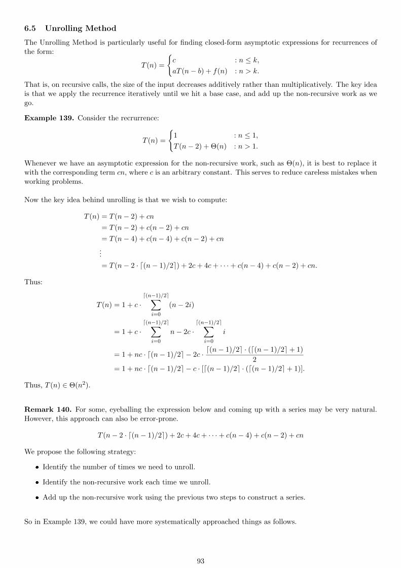
6.5 Unrolling Method

The Unrolling Method is particularly useful for finding closed-form asymptotic expressions for recurrences ofthe form:

T (n) =

c : n ≤ k,aT (n− b) + f(n) : n > k.

That is, on recursive calls, the size of the input decreases additively rather than multiplicatively. The key ideais that we apply the recurrence iteratively until we hit a base case, and add up the non-recursive work as wego.

Example 139. Consider the recrurrence:

T (n) =

1 : n ≤ 1,

T (n− 2) + Θ(n) : n > 1.

Whenever we have an asymptotic expression for the non-recursive work, such as Θ(n), it is best to replace itwith the corresponding term cn, where c is an arbitrary constant. This serves to reduce careless mistakes whenworking problems.

Now the key idea behind unrolling is that we wish to compute:

T (n) = T (n− 2) + cn

= T (n− 2) + c(n− 2) + cn

= T (n− 4) + c(n− 4) + c(n− 2) + cn

...

= T (n− 2 · ⌈(n− 1)/2⌉) + 2c+ 4c+ · · ·+ c(n− 4) + c(n− 2) + cn.

Thus:

T (n) = 1 + c ·⌈(n−1)/2⌉∑

i=0

(n− 2i)

= 1 + c ·⌈(n−1)/2⌉∑

i=0

n− 2c ·⌈(n−1)/2⌉∑

i=0

i

= 1 + nc · ⌈(n− 1)/2⌉ − 2c · ⌈(n− 1)/2⌉ · (⌈(n− 1)/2⌉+ 1)

2= 1 + nc · ⌈(n− 1)/2⌉ − c · [⌈(n− 1)/2⌉ · (⌈(n− 1)/2⌉+ 1)].

Thus, T (n) ∈ Θ(n2).

Remark 140. For some, eyeballing the expression below and coming up with a series may be very natural.However, this approach can also be error-prone.

T (n− 2 · ⌈(n− 1)/2⌉) + 2c+ 4c+ · · ·+ c(n− 4) + c(n− 2) + cn

We propose the following strategy:

Identify the number of times we need to unroll.

Identify the non-recursive work each time we unroll.

Add up the non-recursive work using the previous two steps to construct a series.

So in Example 139, we could have more systematically approached things as follows.

93

1. We subtract 2 from the size of the input each time we unroll. So we hit a base case when:

n− 2k ≤ 1.

Solving for k, we obtain:k ≥ (n− 1)/2.

So k = ⌈(n− 1)/2⌉.

2. When we substitute T (n − 2i) using the recurrence, we obtain the term T (n − 2(i + 1)) + c(n − 2i).Therefore, the non-recursive work is c(n− 2i) (where i ≥ 0 is an integer).

3. It follows that:

T (n) = (cost of base case) · (number of times the base case is reached) + c ·⌈(n−1)/2⌉∑

i=0

(n− 2i)

= 1 · 1 + c ·⌈(n−1)/2⌉∑

i=0

n− 2c ·⌈(n−1)/2⌉∑

i=0

i

= 1 + nc · (⌈(n− 1)/2⌉+ 1)− 2c · ⌈(n− 1)/2⌉ · (⌈(n− 1)/2⌉+ 1)

2= 1 + nc · (⌈(n− 1)/2⌉+ 1)− c · [⌈(n− 1)/2⌉ · (⌈(n− 1)/2⌉+ 1)].

Thus, we have that T (n) ∈ Θ(n2).

Example 141. We consider a second example. Let:

T (n) =

1 : n < 2,

2T (n− 3) + 5 : n ≥ 2.

We proceed as follows.

1. We first determine the number of times that we need to unroll. We hit a base case when n − 3k < 2.Solving for k, we obtain that:

k > (n− 2)/3.

So we have to unroll until k = ⌈(n− 2)/3⌉.

2. When we unroll T (n− 3i), we obtain 2T (n− 3(i+ 1)) + 5. Note that when we unroll 2T (n− 3(i+ 1)),we obtain 2 · [2T (n− 3(i+ 2))) + 5]. So:

T (n− 3i) = 2 · [2T (n− 3(i+ 2))) + 5] + 5

= 22T (n− 3(i+ 2))) + 2 · 5 + 20 · 5.

We intentionally left the coefficients as 22, 2, and 20 respectively, to emphasize a pattern.

3. Thus:

T (n) = (cost of base case) · (number of times the base case is reached) +

⌈(n−2)/3⌉∑i=0

2i · 5

= 1 · 2⌈(n−2)/3⌉ + 5 ·⌈(n−2)/3⌉∑

i=0

2i

= 2⌈(n−2)/3⌉ + 5 · 2⌈(n−2)/3⌉+1 − 1

2− 1

= 2⌈(n−2)/3⌉ + 5 · (2⌈(n−2)/3⌉+1).

Taking the high-order term, we obtain that T (n) ∈ Θ(2⌈(n−2)/3⌉+1) = Θ(2n/3).

94

6.6 Tree Method

The tree method is particularly useful for analyzing recurrences of the form T (n) = aT (n/b)+f(n). Intuitively,we may use a tree structure to model the recursive calls of the method. A recurrence of the form T (n) =aT (n/b) + f(n) indicates that a function makes a recursive calls, where each such call has input of size n/b.The non-recursive work at the initial call is f(n). The key idea is to identify the non-recursive work at eachlevel of the tree, and then add up said work.

Example 142. Recall the recurrence for Mergesort:

T (n) =

Θ(1) : n ≤ 10,

2T (n/2) + Θ(n) : n > 1.

The first thing we do is replace Θ(1) with a constant c1 and Θ(n) with c2n. We do this for clarity, as well asto remove a common place for errors and misconceptions to occur. So effectively, we now have the recurrence:

T (n) =

c1 : n ≤ 1,

2T (n/2) + c2n : n > 1.

We use a tree diagram to help us spot the pattern. Note that the tree extends much further than the initialfew levels, but the initial few levels are usually enough to helps us spot a pattern.

c2n

c2(n/2)

c2(n/4) c2(n/4)

c2(n/2)

c2(n/4) c2(n/4)

Observe that at level i of the tree, the non-recursive work associated with the given method call (node on thetree) is c2n/2

i. Furthermore, there are 2i nodes at level i. So the total non-recursive work at level i is:

c2(n/2i) · 2i = c2n.

We now determine the number of levels of the tree. Let k denote the number of levels of the tree. We willsolve for k. The leaf nodes correspond to base cases. So we hit a base case when: n/2k ≤ 1; or equivocally,when n ≤ 2k. Thus, k ≤ log2(n). As the number of levels of the tree is an integer, we take:

k = ⌈log2(n)⌉.

Thus, the total work performed by Mergesort is:

T (n) ≤⌈log2(n)⌉∑

i=0

c2n

= c2n · ⌈log2(n)⌉.

Thus, T (n) ∈ O(n log(n)). We will show on homework that this bound is actually tight, and so T (n) ∈Θ(n log(n)).

Remark 143. The tree diagram may be useful in spotting patterns, but it is not required on homework. Thekey pieces of information include the cost of the non-recursive work at each call (i.e., at each node), as well asthe number of levels in the tree. Using these pieces of information, we can determine the asymptotic runtimecomplexity.

95

Example 144. Consider the recurrence:

T (n) =

1 : n < 2,

3T (n/2) + n/3 : n ≥ 2.

We wish to determine a tight asymptotic bound on T (n). To this end, we employ the tree method. We identifythe non-recursive work at each level, as well as the number of levels. To help us identify the non-recursive workat each level, we use a tree diagram. Of course, the tree proceeds for many more levels, but we draw only thefirst few to help us spot the pattern.

n/3

n

2 · 3

n

22 · 3n

22 · 3n

22 · 3

n

2 · 3

n

22 · 3n

22 · 3n

22 · 3

n

2 · 3

n

22 · 3n

22 · 3n

22 · 3

Observe that at level i, the non-recursive work identified in a given node is n/(2i ·3). We intentionally leave 2i ·3factored, as this will be useful for evaluating a geometric series that we will see later. To be more suggestivethat n/3 is the constant for our geometric series, we write this as:

n

3· 12i.

Now at level i, there are 3i nodes. So the total non-recursive work done at level i of the tree is:

n

3· 3

i

2i.

We now determine the number of levels of the tree. We hit a base case when n/2k < 2; or equivocally, whenn < 2k+1. So log2(n) < k + 1, or k > log2(n)− 1. Thus, the tree has k = ⌈log2(n)− 1⌉ levels.

Thus:

T (n) =

⌈log2(n)−1⌉∑i=0

n

3·(3

2

)i

=n

3

⌈log2(n)−1⌉∑i=0

·(3

2

)i

=n

3

[1− (3/2)⌈log2(n)−1⌉+1

1− (3/2)

]=n

3· 2 ·

[(3/2)⌈log2(n)−1⌉+1

]=

2n

3·[(3/2)⌈log2(n)⌉

]=

2n

3·[(3/2)⌈log3/2(n)/ log3/2(2)⌉

]=

2n

3·[n⌈1/ log3/2(2)⌉

]So T (n) ∈ Θ

(n1+⌈1/ log3/2(2)⌉

).

96

7 Divide and Conquer

In this section, we introduce the Divide and Conquer strategy. The key approach is to divide a problem up intosmaller, disjoint instances of the same problem. We then solve the smaller problems and use those solutions toobtain a solution for our original instance. As a result, Divide and Conquer approaches are often amenable toparallelization. In particular, the Divide and Conquer strategy arises naturally in designing (Boolean) circuits,which constitute the standard model for parallel computation. Both parallel and distributed computing, aswell as circuit complexity, extend beyond the scope of the course, and we will not discuss them further here.

We have already seen an example of the Divide and Conquer paradigm with Mergesort. Here, the key strategywas to divide the array into two sub-arrays. We then sorted the sub-arrays and merged those into a single,sorted array. We now consider a second divide and conquer sorting algorithm: Quicksort. While Quicksortdoes not achieve the same worst-case runtime complexity of Θ(n log(n)) that Mergesort achieves, Quicksort ismuch faster in practice than Mergesort. Additionally, Quicksort has an average runtime of Θ(n log(n)).

7.1 Deterministic Quicksort

The key idea behind Quicksort is to select an element x of our array and rearrange the elements so that theelements smaller than x are to the left of x, and the elements that are larger than x are to the right of x. Wethen recursively sort the left and right sub-arrays. We begin by introducing the partition subroutine.

Algorithm 16 Partition

1: procedure Parition(Array A[1, . . . , n], Integer start, Integer end)2: i← start3: for j ← start; j ≤ end− 1; j ← j + 1 do4: if A[j] ≤ A[end] then5: Swap(A, i, j)6: i← i+ 1

7: Swap(A, i, e) return i

Example 145. Suppose we wish to Partition([2, 6, 5, 1, 4, 3], 1, 6). So here, start = 1 and end = 6. Weproceed as follows.

(a) We set i ← 1 and j ← 1. Here, A[j] = 2 . As A[j] ≤ A[end] = 3, we swap A[i] and A[j]. As i = j = 1,the state of the array is not modified. We now update i← i+ 1, as per line 6 of the algorithm. We alsoupdate j ← j + 1 at the end of the first iteration of the loop.

(b) Now here, we have i = j = 2 and A[j] = 6. As A[j] ≤ A[end] = 3, the if statement on line 4 is notexecuted. So we set j ← j + 1 and proceed to the next iteration of the loop.

(c) Now here, we have i = 2, j = 3, and A[j] = 5. As A[j] ≤ A[end] = 3, the if statement on line 4 is notexecuted. So we set j ← j + 1 and proceed to the next iteration of the loop.

(d) Now here, we have i = 2, j = 4, and A[j] = 1. As A[j] ≤ A[end] = 3, we swap A[i] and A[j]. SoA = [2, 1, 5, 6, 4, 3]. We now increment i← i+1, as per line 6 of the algorithm. We also update j ← j+1at the end of the first iteration of the loop.

(e) Now here, we have i = 3, j = 5, and A[j] = 4. As A[j] ≤ A[end] = 3, the if statement on line 4 is notexecuted. So we set j ← j + 1. Now j = 6, so the loop terminates.

(f) At our last step, we have we have i = 3, j = 6, and A[j] = 3. As A[j] = A[end], we swap A[i] and A[j].So A = [2, 1, 3, 6, 4, 5]. The algorithm terminates, returning i = 3.

Example 146. Suppose we wish to Partition([1, 4, 3, 6, 5, 2], 1, 6). So here, start = 1 and end = 6. Weproceed as follows.

We set i ← 1 and j ← 1. Here, A[j] = 1. As A[j] ≤ A[end] = 2, we swap A[i] and A[j]. As i = j = 1,the state of the array is not modified. We now update i← i+ 1, as per line 6 of the algorithm. We alsoupdate j ← j + 1 at the end of the first iteration of the loop.

97

Now here, we have i = j = 2 and A[j] = 4. As A[j] ≤ A[end] = 2, the if statement on line 4 is notexecuted. So we set j ← j + 1 and proceed to the next iteration of the loop.

Now here, we have i = 2, j = 3, and A[j] = 3. As A[j] ≤ A[end] = 2, the if statement on line 4 is notexecuted. So we set j ← j + 1 and proceed to the next iteration of the loop.

Now here, we have i = 2, j = 4, and A[j] = 6. As A[j] ≤ A[end] = 2, the if statement on line 4 is notexecuted. So we set j ← j + 1 and proceed to the next iteration of the loop.

Now here, we have i = 2, j = 5, and A[j] = 5. As A[j] ≤ A[end] = 2, the if statement on line 4 is notexecuted. So we set j ← j + 1. Now j = 6, so the loop terminates.

At our last step, we have i = 2, j = 6, and A[j] = 2. As A[j] = A[end] = 2, we swap A[i] and A[j]. SoA = [1, 2, 3, 6, 5, 4]. The algorithm terminates, returning i = 2.

We now turn to formalizing Quicksort.

Algorithm 17 Quicksort

1: procedure Quicksort(Array A[1, . . . , n], Integer start, Integer end)2: if start < end then3: q ← Partition(A, start, end)4: Quicksort(A, 1, q − 1)5: Quicksort(A, q + 1, end)

Example 147. We wish to use Quicksort to sort A = [2, 6, 5, 1, 4, 3]. Here, we invoke Quicksort(A, 1, 6). Sostart = 1 and end = 6. We proceed as follows. Note that for the Partition calls, ony the result will beshown.

(a) We partition the array, invoking Partition(A, 1, 6). We note that the call to Partition updates A =[2, 1, 3, 6, 4, 5] and returns q = 3. So we recursively invoke Quicksort(A, 1, 2) and Quicksort(A, 3, 6).

(b) We consider Quicksort(A, 1, 2). Here, we wish to sort A[1, 2] = [2, 1]. Now Partition(A, 1, 2) selects 1as the pivot and returns the index q = 1, with A = [1, 2, 3, 6, 4, 5]. So now we have start = 1, end = 2,and q = 1. So the subsequent recursive calls Quicksort(A, 1, 1) and Quicksort(A, 2, 2) are base cases.So no further modifications to A are made here.

(c) We now consider Quicksort(A, 4, 6). So we wish to sort the subarray A[4, . . . , 6] = [6, 4, 5]. The call toPartition(A, 4, 6) selects 5 as the pivot and returns q = 5, with A = [1, 2, 3, 4, 5, 6]. So start = 4, end = 6,and q = 5. So the subsequent recursive calls Quicksort(A, 4, 4) and Quicksort(A, 6, 6) are base cases.So no further modifications to A are made here.

(d) The algorithm terminates, and the array is sorted: A = [1, 2, 3, 4, 5, 6].

We now examine the worst-case complexity of Quicksort. In order for Quicksort to be effective, we need tomake progress on sorting two sub-arrays of comparable size. In the extreme case, the pivot element has nothingto its right (or nothing to its left) after the partition step. This yields the following recurrence:

T (n) =

Θ(1) : n ≤ 1,

T (n− 1) + Θ(n) : n > 1.

Here, the Θ(n) term for the non-recursive work arises from the complexity of the Partition function. Sounrolling this recurrence, we obtain that T (n) ∈ Θ(n2).

98

7.2 Randomized Quicksort

In this section, we consider a randomized implementation of Quicksort. The key idea is that we select a randomelement of the array as our pivot. We then swap this random element so that it is at the end of the array, andthen proceed with the partitioning procedure. The expected runtime of this procedure is O(n log(n)). Ourproof is adapted from [IS10].

Theorem 148. Let A[1, . . . , n] be an array of length n, and suppose we select a pivot uniformly at random.Then the expected runtime of the randomized Quicksort procedure is O(n log(n)).

Proof. As we only care about the relative order of the elements, we may assume that A contains preciselythe elements of 1, . . . , n in some order. For each i, j ∈ 1, . . . , n, let Xij denote the event that Quicksortcompares i and j. Let X denote the random variable denoting the number comparisons that Quicksort makes.As no pair of elements are compared twice, we have that:

X =n∑

i=1

n∑j=i+1

Xij .

Our goal is to determine the expected number of comparisons, E[X]. By the linearity of expectation, we havethat:

E[X] =

n∑i=1

n∑j=i+1

E[Xij ]

=n∑

i=1

n∑j=i+1

Pr[Quicksort compares i, j].

We now determine Pr[Quicksort compares i, j].Without loss of generality, suppose i < j. We note that we onlycompare elements of the array to the pivot. Now if we select an element x ∈ i+1, . . . , j− 1 as a pivot beforei or j, then i and j belong to separate sub-arrays and are not compared on recursive calls to Quicksort. Hence,i and j are compared if and only if either i or j is selected as the pivot before any element of i+1, . . . , j− 1.As the pivots are selected uniformly at random, we have that the probability that i or j is selected as a pivotbefore any element of i+ 1, . . . , j − 1 is:

Pr[Quicksort compares i, j] =2

|i, . . . , j|=

2

j − i+ 1.

It follows that:

n∑i=1

n∑j=i+1

Pr[Quicksort compares i, j] =n∑

i=1

n∑j=i+1

2

j − i+ 1

= 2n∑

i=1

n∑j=i+1

1

j − i+ 1

≤ 2n∑

i=1

n∑j=i

1

j

= 2n

n∑j=1

1

j

≤ 2n ·∫ n

1

1

xdx

= 2n ln(n).

So the randomized Quicksort procedure makes at most 2n ln(n) comparisons. Hence, randomized Quicksorthas expected runtime O(n log(n)), as desired.

99

8 Dynamic Programming

Dynamic programming is a powerful technique to solve computational problems, which have a recursive sub-structure and recurring subproblems. The idea is to solve these recursive subcases and store these solutions ina lookup table. When a solved recursive subcase is encountered, the existing solution is accessed using onlya constant number of steps. A solution to the initial instance is constructed from the solutions to the sub-cases, typically in a bottom-up manner. Frequently, the computational problems of interest are optimizationproblems. We begin by introducing some examples amenable to the dynamic programming technique.

8.1 Rod-Cutting Problem

In this section, we examine the Rod-Cutting Problem. Let us consider a motivating example. Suppose wehave a rod of length 5, which can be cut into smaller pieces of integer lengths 1, 2, 3, or 4. These smaller rodscan then be further cut into smaller pieces. We stress that the rod pieces can only be cut into pieces of integerlength; so pieces of size 1/2 or π are not considered in this problem. Now suppose that we can sell rods oflength 1 for $1, which we denote p1 = 1. Similarly, suppose that the prices for rods of length 2, . . . , 5 are givenby p2 = 4, p3 = 7, p4 = 8, and p5 = 9 respectively. We make two key assumptions: we will sell all the smallerrods, regardless of the cuts; and that each cut is free. Under these assumptions, how should the rod be cut tomaximize the profit? We note the following cuts and the corresponding profits.

If the rod is cut into five pieces of length 1, we stand to make 5 · p1 = $5.

If the rod is cut into one piece of length 2 and one piece of length 3, we stand to make p2+p3 = 4+7 = $11.

If the rod is cut into two pieces of length 2 and one piece of length 1, we stand to make 2 · p2 + p1 =8 + 1 = $9.

Out of the above options, cutting the rod into one piece of length 2 and one rod of length 3 is the mostprofitable. Of course, there are other possible cuts not listed above, such as cutting the rod into one pieceof length 1 and one piece of length 4. The goal is to determine the most profitable cut. The Rod-CuttingProblem is formalized as follows.

Definition 149 (Rod-Cutting Problem).

Instance: Let n ∈ N be the length of the rod, and let p1, p2, . . . , pn be non-negative real numbers. Here,pi is the price of a length i rod.

Solution: The maximum revenue, which we denote rn, obtained by cutting the rod into smaller piecesof integer lengths and selling the smaller rods.

Intuitively, the maximum revenue is determined by examining the revenues for the subdivisions and taking thelargest. Mathematically, this amounts to the following expression:

rn = max(pn, r1 + rn−1, r2 + rn−2, . . . , rn−1 + r1). (30)

We begin by working through an example of utilizing dynamic programming to determine the maximum profit.

Example 150. Suppose we have a rod of length 5, with prices p1 = 1, p2 = 4, p3 = 7, p4 = 8, p5 = 9. Weproceed as follows.

(a) Initialize a lookup table T [1, . . . , 5]. Now for a rod of length 1, there is only one price: p1. So we setT [1] := p1.

(b) Now consider a rod of length 2. There are two options: either don’t cut the rod, or cut the rod into twosmaller pieces of length 1. Here, p2 = 4 represents the case in which no cuts to a rod of length 2. Nowsuppose instead we cut the rod up into two smaller pieces each of length 1. We know that the maximumprofit for a rod of length 1 is r1 = T [1] = 1. So the profit of cutting the rod into two smaller pieces eachof length 1 is 2r1 = 2. Now r2 = max(p2, 2r1) = 4, so we set T [2] = 4.

(c) Now consider a rod of length 3. Here, we have more options: we can leave the rod untouched, we candivide the rod into smaller pieces of length 1 or length 2; or we can divide the rod into three pieces oflength 1. If we do not divide the rod into smaller pieces, the profit is p3 = 7. Now suppose we divide

100

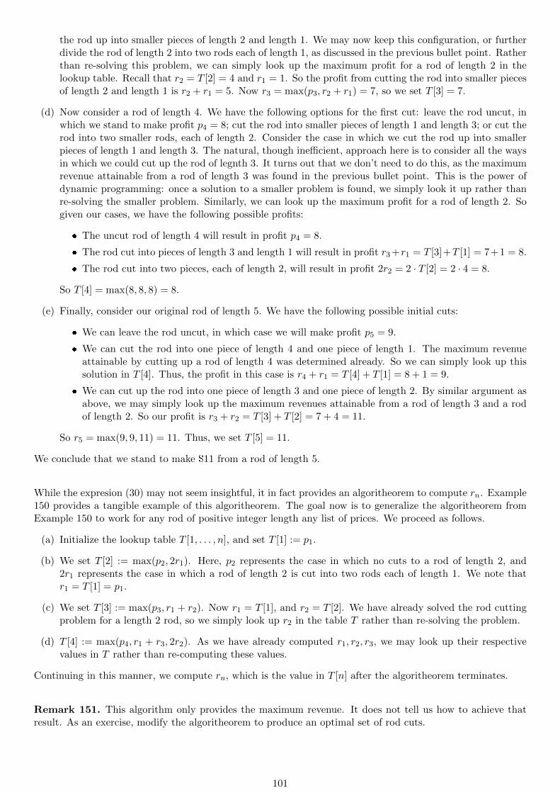
the rod up into smaller pieces of length 2 and length 1. We may now keep this configuration, or furtherdivide the rod of length 2 into two rods each of length 1, as discussed in the previous bullet point. Ratherthan re-solving this problem, we can simply look up the maximum profit for a rod of length 2 in thelookup table. Recall that r2 = T [2] = 4 and r1 = 1. So the profit from cutting the rod into smaller piecesof length 2 and length 1 is r2 + r1 = 5. Now r3 = max(p3, r2 + r1) = 7, so we set T [3] = 7.

(d) Now consider a rod of length 4. We have the following options for the first cut: leave the rod uncut, inwhich we stand to make profit p4 = 8; cut the rod into smaller pieces of length 1 and length 3; or cut therod into two smaller rods, each of length 2. Consider the case in which we cut the rod up into smallerpieces of length 1 and length 3. The natural, though inefficient, approach here is to consider all the waysin which we could cut up the rod of legnth 3. It turns out that we don’t need to do this, as the maximumrevenue attainable from a rod of length 3 was found in the previous bullet point. This is the power ofdynamic programming: once a solution to a smaller problem is found, we simply look it up rather thanre-solving the smaller problem. Similarly, we can look up the maximum profit for a rod of length 2. Sogiven our cases, we have the following possible profits:

The uncut rod of length 4 will result in profit p4 = 8.

The rod cut into pieces of length 3 and length 1 will result in profit r3+r1 = T [3]+T [1] = 7+1 = 8.

The rod cut into two pieces, each of length 2, will result in profit 2r2 = 2 · T [2] = 2 · 4 = 8.

So T [4] = max(8, 8, 8) = 8.

(e) Finally, consider our original rod of length 5. We have the following possible initial cuts:

We can leave the rod uncut, in which case we will make profit p5 = 9.

We can cut the rod into one piece of length 4 and one piece of length 1. The maximum revenueattainable by cutting up a rod of length 4 was determined already. So we can simply look up thissolution in T [4]. Thus, the profit in this case is r4 + r1 = T [4] + T [1] = 8 + 1 = 9.

We can cut up the rod into one piece of length 3 and one piece of length 2. By similar argument asabove, we may simply look up the maximum revenues attainable from a rod of length 3 and a rodof length 2. So our profit is r3 + r2 = T [3] + T [2] = 7 + 4 = 11.

So r5 = max(9, 9, 11) = 11. Thus, we set T [5] = 11.

We conclude that we stand to make $11 from a rod of length 5.

While the expresion (30) may not seem insightful, it in fact provides an algoritheorem to compute rn. Example150 provides a tangible example of this algoritheorem. The goal now is to generalize the algoritheorem fromExample 150 to work for any rod of positive integer length any list of prices. We proceed as follows.

(a) Initialize the lookup table T [1, . . . , n], and set T [1] := p1.

(b) We set T [2] := max(p2, 2r1). Here, p2 represents the case in which no cuts to a rod of length 2, and2r1 represents the case in which a rod of length 2 is cut into two rods each of length 1. We note thatr1 = T [1] = p1.

(c) We set T [3] := max(p3, r1 + r2). Now r1 = T [1], and r2 = T [2]. We have already solved the rod cuttingproblem for a length 2 rod, so we simply look up r2 in the table T rather than re-solving the problem.

(d) T [4] := max(p4, r1 + r3, 2r2). As we have already computed r1, r2, r3, we may look up their respectivevalues in T rather than re-computing these values.

Continuing in this manner, we compute rn, which is the value in T [n] after the algoritheorem terminates.

Remark 151. This algorithm only provides the maximum revenue. It does not tell us how to achieve thatresult. As an exercise, modify the algoritheorem to produce an optimal set of rod cuts.

101

8.2 Recurrence Relations

The key aspect in designing a dynamic programming algorithm is to identify the recursive structure. Inparticular, finding an explicit recurrence informs us as to the lookup table, as well as the natural strategy tofill in the lookup table. In this section, we discuss strategies for identifying recurrence relations. We will usecombinatorics to explore these ideas. Our exposition is adopted from [Loe18].

Suppose we are interested in counting sets of combinatorial objects. And suppose we have several relatedfamilies of objects, which we label T0, T1, . . . , Tn, . . .. Here, we think of the index n as measuring the size of theobjects in Tn (e.g., the set of rooted binary trees on n vertices). It is sometimes possible to explicitly describethe objects in Tn, such as with the sum and product rules, to arrive at a closed-form expression for |Tn|, thenumber of elements in Tn. Other times, it is more natural to describe a construction for the objects in Tnusing smaller objects from the sets T0, . . . , Tn−1. Such arguments are inherent in the dynamic programmingparadigm, and they lead to natural recursive formulas which describe the number of viable solutions (or ifthere even is a viable solution).

We illustrate this technique below.

Example 152. Let Wn be the set of all words ω ∈ 0, 1n such that there is no substring of the form 00 inω. Let fn := |Wn|. Our first step is to describe the initial conditions. Observe that W0 = ε, where ε is thestring of length 0, and W1 = 0, 1. So f0 = 0 and f1 = 2.

Now consider a string ω ∈ Wn of length n ≥ 2. We note that the first character ω0 ∈ 0, 1. Consider thefollowing cases.

Case 1: If ω1 = 0, then necessarily ω2 = 1; otherwise, we would have a 00 substring. So ω = 01τ , whereτ ∈ Wn−2. There are fn−2 = |Wn−2| ways to select τ . So there are fn−2 such strings ω of the form 01τin Wn.

Case 2: If ω1 = 1, then the second character may be either 0 or 1. In this case, ω = 0τ , where τ ∈Wn−1.So we have fn−1 such ways to select ω in this case.

As Cases 1 and 2 are disjoint, we have that fn = fn−1 + fn−2, with the initial conditions that f0 = 1 andf1 = 2.

Example 153. Recall from Discrete Math that(nk

)counts the number of k-element subsets of 1, . . . , n. We

derive a recurrence for(nk

)by counting the number of ways to construct a k-element set S. We first ascertain

the base cases. We set(nk

):= 0 whenever k < 0 or k > n.

Case 1: Suppose that 1 ∈ S. In this case, we must select the remaining n − 1 elements of S from2, . . . , n. There are n − 1 such elements from which to choose, and we want a k − 1 element setS′ ⊆ 2, . . . , n such that S = 1 ∪ S′. There are

(n−1k−1

)such sets.

Case 2: Suppose that 1 ∈ S. So we select S ⊆ 2, . . . , n. There are n− 1 such elements from which tochoose, and we would like a k-element set. So there are

(n−1k−1

)such ways to select S.

So the total number of ways to select a k-element set from 1, . . . , n is(nk

)=

(n−1k

)+(n−1k−1

).

Example 154. Consider an n ×m rectangle, where n,m ≥ 0. So we have n rows and m columns. We startat the origin (0, 0), with the goal of reaching (m,n). We may only move one cell to the left or one cell up at atime. That is, we may move from (x, y) to (x+ 1, y) or (x, y + 1). We now count the number of ways to reach(m,n). Denote this recurrence L(m,n). Observe that when either n = 0 or m = 0, there is only one such path.So L(m, 0) = L(0, n) = 1.

Now consider L(m,n). Here, if we move one cell up, then we have an (n − 1) × m rectangle, which yieldsL(m,n− 1) such paths. If we instead move one cell to the left, then we have an n× (m− 1) rectangle, whichyields L(m− 1, n) such paths. These choices are disjoint, so we have the recurrence:

L(n,m) =

1 : n = 0 or m = 0,

L(n− 1,m) + L(n,m− 1) : n,m > 1.

102

8.3 Longest Common Subsequence

In this section, we introduce the Longest Common Subsequence Problem, which is also amenable to the dynamicprogramming technique. Unlike other dynamic programming problems, the Longest Common SubsequenceProblem utilizes a two-dimensional table rather than a one-dimensional array. The purpose of this section isto illustrate the usage of multidimensional lookup tables in dynamic programming problems. To this end, theLongest Common Subsequence Problem serves as a tangible example. We begin by formalizing the LongestCommon Subsequence Problem.

Definition 155 (Subsequence). Let Σ be a finite set, which we refer to as an alphabet. Let ω ∈ Σn be a stringof length n (so each letter of ω belongs to Σ). We say that ψ ∈ Σm is a subsequence of ω if there exists astrictly increasing sequence of indices (i1, i2, . . . , im) such that ωik = ψk for all k ∈ [m].

Example 156. Let ω = (A,B,C,B,D,A,B), and let ψ = (A,C,D,B). We indicate how ψ is realized as asubsequence of ω by bolding the appropriate letters:

(A, B,C, B,D, A,B).

Note that the letters of ψ need to appear in the same order in ω; that is, the selected A must appear beforethe selected C, which then appears before the selected D, and so on. However, the letters of ψ need not beconsecutive or contiguous in ω. Consider the sequence of indices (1, 3, 5, 7). So ψ1 = ω1, ψ2 = ω3, ψ3 = ω5, andψ4 = ω7. Thus, ψ is a subsequence of ω.

Definition 157 (Common Subsequence). Let Σ be an alphabet. Let ω ∈ Σn, τ ∈ Σm be sequences. We saythat ψ ∈ Σℓ is a common subsequence of ω and τ if: ψ is a subsequence of ω, and ψ is a subsequence of τ .Note that ψ does not have to appear as a subsequence in the same position in both ω and τ .

Example 158. Let ω = (0, 2, 1, 2, 3, 0, 1) and τ = (2, 3, 1, 0, 2, 0). The sequence (2, 1, 0) is a subsequence ofboth ω and τ . Here, (2, 1, 0) appears in ω at the indices (2, 3, 6). That is, (2, 1, 0) appears in ω as follows:

(0,2,1, 2, 3,0, 1).

Similarly, (2, 1, 0) appears in τ at the indices (1, 3, 4). That is, (2, 1, 0) is realized as a subsequence of τ asfollows:

(2, 3,1, 0, 2, 0)

Definition 159 (Longest Common Subsequence Problem (LCS)).

Instance: Let Σ be an alphabet, and let ω ∈ Σn, τ ∈ Σm be sequences of length n and m respectively.

Solution: A sequence ψ that is common to both ω and τ ; and for any other common subsequence σ ofω and τ , |σ| ≤ |ψ|.

The naıve approach to solving LCS is enumerating all the possible subsequences of σ and τ , and recordingthe longest. Without loss of generality, suppose that m ≤ n. So there are 2m possible index sequences tocheck, which correspond bijectively to subsequences of τ . So for large sequences, the brute force and ignorancesolution is not a practical solution. The dynamic programming approach provides a linear time algoritheoreminstead.

Dynamic programming works best when optimal solutions to subproblems can be used to construct an optimalsolution to the original instance. We first show that LCS exhibits this property.

Theorem 160. Let Σ be an alphabet, and let ω ∈ Σn, τ ∈ Σm be sequences. Let ψ ∈ Σk be a longest commonsubsequence of ω and τ . The following hold:

(a) If ωn = τm, then ψk = ωn = τn and ψ[1, . . . , k − 1] is a longest common subsequence of ω[1, . . . , n − 1]and τ [1, . . . ,m− 1].

(b) If ωn = τm and ψk = ωn, then ψ is a longest common subsequence of ω[1, . . . , n− 1] and τ . Similarly, ifωn = τm and ψk = τm, then ψ is a longest common subsequence of ω and τ [1, . . . ,m− 1].

Proof.

103

(a) Let σ be a common subsequence of ω and τ whose last digit does not correspond to the last instance ofthe character ωn = τm in ω and τ . Then σ can be augmented by appending the character ωn = τm. Soevery longest common subsequence of ω and τ has last character ωn = τm.

We now show that ψ[1, . . . , k− 1] is a longest common subsequence of ω[1, . . . , n− 1] and τ [1, . . . ,m− 1].Observe that ψ[1, . . . , k − 1] is a common subsequence of ω[1, . . . , n − 1] and τ [1, . . . ,m − 1]. Supposeto the contrary that there exists a longest common subsequence σ of ω[1, . . . , n− 1] and τ [1, . . . ,m− 1],with |σ| > k. Then σ can be augmented with ωn = τm to obtain a common subsequence of ω and τ .This contradicts the assumption that any longest common subsequence of ω and τ has length k. Soψ[1, . . . , k − 1] is a longest common subsequence of ω[1, . . . , n− 1] and τ [1, . . . ,m− 1].

(b) Suppose that ωn = τm. Now suppose that ψk = ωn. We show that ψ is a longest common subsequence ofω[1, . . . , n− 1] and τ , by contradiction. Let σ be a longest common subsequence of ω[1, . . . , n− 1] and τof length |σ| > k. Clearly, σ is a common subsequence of ω and τ . Now |σ| > |ψ| = k, contradicting theassumption that ψ was a longest common subsequence of ω and τ . So ψ is a longest common subsequenceof ω and τ . Interchanging the roles of ω and τ , we obtain that: if ωn = τm and ψk = τm, then ψ is alongest common subsequence of ω and τ [1, . . . ,m− 1].

Theorem 160 provides the insights necessary for designing a dynamic programming algoritheorem to solve LCS.Let ω ∈ Σn, τ ∈ Σm be sequences. If ωn = τm, we record the last character and examine the smaller LCSinstance with ω[1, . . . , n− 1] and τ [1, . . . ,m− 1]. If ωn = τm. Otherwise, we need to find the longest commonsubsequences of ω and τ [1, . . . ,m− 1]; and ω[1, . . . , n] and τ . These observations yield a natural recurrence tocompute the length of the longest common subsequence for a pair of strings:

ℓ[i, j] =

0 : i = 0 or j = 0,

ℓ[i− 1, j − 1] + 1 : i, j > 0 and xi = yj ,

max(ℓ[i− 1, j], ℓ[i, j − 1]) : i, j > 0 and xi = yj .

Using the recurrence ℓ[i, j] as a template, we design an explicit dynamic programming algoritheorem. Weproceed as follows.

(a) Let ω ∈ Σn, τ ∈ Σm be our input sequences. We initialize a lookup table T [0, . . . , n][0, . . . ,m] to be atwo-dimensional array, where each cell stores:

A natural number corresponding to the length of a longest common subsequence; and

A pointer to another cell in the lookup table, which corresponds to the optimal subproblem asspecified in Theorem 160.

Now recall that if either of the input sequences have length 0, the length of the longest common subse-quence is 0. Therefore, we set T [i][0] = 0 and T [0][j] = 0 for all i ∈ [n] and all j ∈ [m]. While our originalinput sequences may not have length 0, sequences we encounter in subproblems may indeed have length0.

(b) We now proceed to fill in the remaining cells in a bottom up manner, row-by-row. Each row is filledleft-to-right. The cells T [i][j] are filled as follows.

Case 1: Suppose ωi = τj . By Theorem 160, any longest common subsequence ψ of ω[1, . . . , i] andτ [1, . . . , j] ends with ωi = τj . Furthermore, ψ[1, . . . , |ψ| − 1] is a longest common subsequence ofω[1, . . . , i− 1] and τ [1, . . . , j − 1]. So we take the following actions:

– Set T [i][j].length = T [i− 1][j − 1].length + 1; and

– Set T [i][j].subproblem = T [i− 1][j − 1].

Case 2: Suppose ωi = τj . Theorem 160 tells us that we need to consider the two subproblems, whosesolutions (or at least, their optimal lengths) are stored in: T [i− 1][j] and T [i][j− 1], respectively. IfT [i− 1][j].length ≥ T [i][j − 1].length, we set:

– T [i][j].length = T [i− 1][j].length

– T [i][j].subproblem = T [i− 1][j].

Otherwise, we set:

104

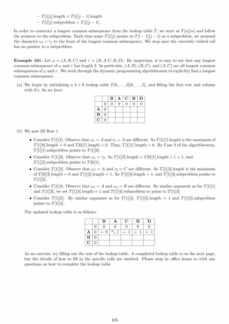
– T [i][j].length = T [i][j − 1].length

– T [i][j].subproblem = T [i][j − 1].

In order to construct a longest common subsequence from the lookup table T , we start at T [n][m] and followthe pointers to the subproblem. Each time some T [i][j] points to T [i− 1][j − 1] as a subproblem, we prependthe character ωi = τj to the front of the longest common subsequence. We stop once the currently visited cellhas no pointer to a subproblem.

Example 161. Let ω = (A,B,C) and τ = (B,A,C,B,D). By inspection, it is easy to see that any longestcommon subsequence of ω and τ has length 2. In particular, (A,B), (B,C), and (A,C) are all longest commonsubsequences of ω and τ . We work through the dynamic programming algoritheorem to explicitly find a longestcommon subsequence.

(a) We begin by initializing a 4 × 6 lookup table T [0, . . . , 3][0, . . . , 5], and filling the first row and columnwith 0’s. So we have:

B A C B D

0 0 0 0 0 0

A 0

B 0

C 0

(b) We now fill Row 1.

Consider T [1][1]. Observe that ω1 = A and τ1 = A are different. So T [1][1].length is the maximum ofT [1][0].length = 0 and T [0][1].length = 0. Thus, T [1][1].length = 0. By Case 2 of the algoritheorem,T [1][1].subproblem points to T [1][0].

Consider T [1][2]. Observe that ω1 = τ2. So T [1][2].length = T [0][1].length + 1 = 1, andT [1][2].subproblem points to T [0][1].

Consider T [1][3]. Observe that ω1 = A and τ3 = C are different. So T [1][3].length is the maximumof T [0][3].length = 0 and T [1][2].length = 1. So T [1][3].length = 1, and T [1][3].subproblem points toT [1][2].

Consider T [1][4]. Observe that ω1 = A and ω4 = B are different. By similar argument as for T [1][1]and T [1][3], we set T [1][4].length = 1 and T [1][4].subproblem to point to T [1][3].

Consider T [1][5]. By similar argument as for T [1][4], T [1][5].length = 1 and T [1][5].subproblempoints to T [1][4].

The updated lookup table is as follows:

B A C B D

0 0 0 0 0 0

A 0 ← 0 1 ← 1 ← 1 ← 1

B 0

C 0

As an exercise, try filling out the rest of the lookup table. A completed lookup table is on the next page,but the details of how to fill in the specific cells are omitted. Please stop by office hours to with anyquestions on how to complete the lookup table.

105

(c) We next fill Rows 2-3, omitting the detailed explanation associated with filling Row 1. The completedlookup table is as follows.

B A C B D

0 0 0 0 0 0

A 0 ← 0 1 ← 1 ← 1 ← 1

B 0 1 ← 1 ← 1 2 ← 2

C 0 ↑ 1 ↑ 1 2 ← 2 ← 2

(d) Finally, we construct a longest common subsequence of ω and τ from the lookup table. We start atT [3][5] and follow the arrows, prepending the character at the given index every time we see . So wehave the sequence:

T [3][5]→ T [3][4]→ T [3][3] (Record C)

→ T [2][2]→ T [2][1] (Record B)

→ T [1][0].

After which, we stop, as T [1][0] does not reference any subproblems. So our longest common subsequenceis (B,C), which we identified at the start of this example.

106

8.4 Edit Distance

In this section, we consider the edit distance problem. Our goal in this section is to practice filling in a lookuptable. The exposition is adapted from [CG18].

Fix an alphabet Σ, and let x, y ∈ Σ∗. Our goal is to convert x into y using the minimum number of operations.That is, we wish to find the minimum distance between x ∈ Σn and y ∈ Σm. This problem is motivatedby applications, such as comparing two strands of DNA in bioinformatics. In addition, computing the editdistance is a key dynamic programming algorithm in natural language processing.

In order to compute the edit distance of two strings, we need to introduce the allowed operations, as well thecosts of each operation. Our operations are as follows.

Substitution: We may replace character i in x with a new character. For example, let x = do andy = so. We may replace x[1] = s obtain y.

Indel: An indel operation stands for an insertion/deletion operation. We may insert a new characterinto x, shifting the subsequent characters. Equivocally, we may delete a character from y, shifting thesubsequent characters forward. As an example, x = grand and y = grande differ by a single indeloperation.

Swap: We may swap two consecutive elements in x. So if x = (x1, . . . , xi, xi+1, . . . , xn) and we swapxi, xi+1, then our new string is x = (x1, . . . , xi+1, xi, . . . , xn). As an example, x = thier and y = their

differ by a single swap operation; namely, swapping the pair ie in x.

For our purposes, we take the costs of each operation to be 1. So the distance between two strings under thiscost scheme is known as the Damerau–Levenshtein (DL) distance.

We now turn to identifying a recurrence. Given strings x[1, . . . , n] and y[1, . . . ,m], denote c[i, j] to be theminimum DL distance between x[1, . . . , i] and y[1, . . . , j]. We note that if i = j = 0, then x = y = ε (that is,x and y are both the empty string). In this case, c[i, j] = 0. We now turn to our recursive cases.

Suppose that xi = yj . In this case, we wish to find the DL distance of x[1, . . . , i− 1] and y[1, . . . , j − 1].This is precisely c[i− 1, j − 1].

If x[1, . . . , i] is not empty (that is, if i > 0), we may try to align x[1, . . . , i] to y[1, . . . , j] by simply deletingthe last character of x[1, . . . , i]. In this case, we have cost 1 + c[i− 1, j].

Similarly, if j > 0, then we may simply delete the last character of y[1, . . . , j], and try to align x[1, . . . , i]and y[1, . . . , j − 1]. The cost here is 1 + c[i, j − 1].

If i, j > 0 and xi = xj , we may substitute xi for yj , and then find the DL distance of x[1, . . . , i− 1] andy[1, . . . , j − 1]. This is precisely 1 + c[i− 1, j − 1].

If i, j > 1 and xi−1xi = yjyj−1, we may swap xi−1 and xj . We then find the DL distance of x[1, . . . , i−2]and y[1, . . . , j − 2]. This is precisely 2 + c[i− 2, j − 2].

The case analysis is involved, and the mathematical recursive formula for c[i, j] is quite dense. We omit theformula, as the case analysis suffices to fill in the lookup table. We now turn to consider an example.

Example 162. Suppose we wish to align x = (S, T,E, P ) and y = (A,P,E). As c[i, j] has two variables, wehave a two-dimensional lookup table.

ε A P E

ε

S

T

E

P

We now turn to filling in the lookup table row-by-row.

107

Row ε.

– We consider c[0, 0]. In this case, both strings are ε. So c[0, 0] = 0.

– We consider c[0, 1], where we seek to align ε and A. This can be accomplished with a single indeloperation. So we set c[0, 1] = 1 and have c[0, 1] point to c[0, 0] with a label for indel.

– We consider c[0, 2], where we seek to align ε and (A,P ). This can be accomplished by inserting Pand aligning P and (A,P ). So c[0, 2] = 1 + c[0, 1] = 2. Furthermore, we have c[0, 2] point to c[0, 1]with a label for indel.

– We consider c[0, 3], where we seek to align ε and (A,P,E). This can be accomplished by insertingE and aligning E and (A,P,E). So c[0, 3] = 1 + c[0, 2] = 3. Furthermore, we have c[0, 2] point toc[0, 1] with a label for indel.

The updated table is below.

ε A P E

ε 0indel←−−− 1

indel←−−− 2indel←−−− 3

S

T

E

P

Row S:

– We consider c[1, 0]. Here, we are aligning S and ε, which can be accomplished with a single indeloperation. So we set c[1, 0] = 1 and point upwards.

– We consider c[1, 1]. Here, we are aligning S and A, which can be accomplished with a singlesubstitution operation. So we set c[1, 1] = 1 + c[0, 0] = 1. Now c[1, 1] points diagonally to c[0, 0],and we label this with substitution.

– We consider c[1, 2]. Here, we seek to align S and (A,P ). As S = P , we may either delete S (whichmeans we consider c[0, 2]) or insert P (which means we consider c[1, 1]). As 1 = c[1, 1] < c[0, 2] = 2,we insert P . So c[1, 2] = 2, and we set c[1, 2] to point to c[1, 1] with label indel.

– We consider c[1, 3]. Here, we seek to align S and (A,P,E). As S = E, we may either delete S (whichmeans we consider c[0, 3]) or insert E (which means we consider c[1, 2]). As 2 = c[1, 2] < c[0, 3] = 3,we choose to insert E. So c[1, 3] = 1 + c[1, 2] = 3, and we set c[1, 3] to point to c[1, 2] with labelindel. The updated table is below.

ε A P E

ε 0indel←−−− 1

indel←−−− 2indel←−−− 3

S ↑ indel 1 sub 1indel←−−− 2

indel←−−− 3

T

E

P

Remark 163. By similar arguments as above, the remaining empty cells in columns ε and A correspondto indel operations. we fill them in below.

ε A P E

ε 0indel←−−− 1

indel←−−− 2indel←−−− 3

S ↑ indel 1 sub 1indel←−−− 2

indel←−−− 3

T ↑ indel 2 ↑ indel 2E ↑ indel 3 ↑ indel 3P ↑ indel 4 ↑ indel 4

108

Row T:

– We consider the cell c[2, 2]. Here, we seek to align (S, T ) and (A,P ). As T = P , we may either usean indel operation such as to delete T (in which case we consider c[1, 2] = 2) or P (in which case,we consider c[2, 1] = 2), or a substitution operation to change T to P (in which case, we considerc[1, 1] = 1). We choose the substitution operation. So we set c[2, 2] = 1 + c[1, 1]. Now c[2, 2] pointsto c[1, 1] with label sub.

– We consider the cell c[2, 3]. Here, we seek to align (S, T ) with (A,P,E). As T = E, we mayeither use an indel operation such as to delete T (in which case, we consider c[1, 3] = 3) or E (inwhich case, we consider c[2, 2] = 2), or we may substitute T for E (in which case, we considerc[1, 2] = 2). As c[1, 2] = c[2, 2], we may choose either indel or sub. We opt for deleting E. So we setc[2, 3] = 1 + c[2, 2] = 3, and c[2, 3] points to c[2, 2] with label for index.

ε A P E

ε 0indel←−−− 1

indel←−−− 2indel←−−− 3

S ↑ indel 1 sub 1indel←−−− 2

indel←−−− 3

T ↑ indel 2 ↑ indel 2 sub 2indel←−−− 3

E ↑ indel 3 ↑ indel 3P ↑ indel 4 ↑ indel 4

Row E:

– Consider c[3, 2]. Here, we seek to align (S, T,E) and (A,P ). As E = P , we may either use an indeloperation such as to delete E (in which case, we consider c[2, 2] = 2) or to delete P (in which case,we consider c[3, 1] = 3), or we may use a substitution operation to change E to P (in which case,we consider c[2, 1] = 2). We opt for deleting E. So we set c[3, 2] = 1 + c[2, 2] = 3, and we set c[3, 2]to point to c[2, 2] with label indel.

– Consider c[3, 3]. Here, we seek to align (S, T,E) and (A,P,E). As the end characters agree, we donot modify them. Instead, we consider c[2, 2]. So we simply set c[3, 3] = c[2, 2] and set c[3, 3] topoint to c[2, 2].

The updated lookup table is below.

ε A P E

ε 0indel←−−− 1

indel←−−− 2indel←−−− 3

S ↑ indel 1 sub 1indel←−−− 2

indel←−−− 3

T ↑ indel 2 ↑ indel 2 sub 2indel←−−− 3

E ↑ indel 3 ↑ indel 3 ↑ indel 3 2

P ↑ indel 4 ↑ indel 4

Row P:

– We consider c[4, 2]. Here, we seek to align (S, T,E, P ) with (A,P ). As the end characters agree, weset c[4, 2] = c[3, 1] and set c[4, 2] to point to c[3, 1].

– We consider c[4, 3]. Here, we seek to align (S, T,E, P ) and (A,P,E). We have several options.First, we may swap (E,P ) in (S, T,E, P ) to obtain (S, T, P,E); in this case, we conisder c[2, 1] = 2.Alternatively, as P = E, we may perform an indel operation either deleting P (in which case, weconsider c[3, 3] = 2). We choose the swap operation. So we set c[4, 3] = c[2, 1] + 1 = 3 and point toc[2, 1].

109

ε A P E

ε 0indel←−−− 1

indel←−−− 2indel←−−− 3

S ↑ indel 1 sub 1indel←−−− 2

indel←−−− 3

T ↑ indel 2 ↑ indel 2 sub 2indel←−−− 3

E ↑ indel 3 ↑ indel 3 ↑ indel 3 2

P ↑ indel 4 ↑ indel 4 3 3 swap- point to c[2, 1]

Now to recover an optimal sequence of operations, we can simply follow the arrows. Namely, we do thefollowing:

Substitue S 7→ A. So we now have (S, T,E, P ) 7→ (A, T,E, P ).

Delete the T in (A, T,E, P ) to obtain (A,E, P ).

Swap the (E,P ) substring to obtain (A,P,E).

110

9 Computational Complexity Theory

9.1 Decision Problems

The goal of Computational Complexity Theory is to classify computational problems according to the amountof resources required to solve them. Space and time are the two most common measures of complexity. Timecomplexity measures how many computations are required for a computer to solve decide an instance of theproblem, with respect to the instance’s size. Space complexity is analogously defined for the amount of extraspace a computer needs to decide an instance of the problem, with respect to the instance’s size.

So far, in Algorithms, we have only studied problems which have efficient (polynomial-time) solutions. How-ever, there are numerous practical problems of interest for which it is unkown if efficient solutions exist. Someof these problems include the Traveling Salesman Problem, Protein Folding, Scheduling, and Optimizationproblems. For other problems, such as generalizations of Chess, Checkers, and Go, it has been proven that noefficient algorithms exist. Computational complexity provides a framework to help us understand which prob-lems have efficient solutions and which don’t. For problems that have resisted or don’t have efficient solutions,there are algorithmic techniques to construct approximate solutions in polynomial time. Such algorithms areknown as approximation algorithms.

In this section, we seek to understand the complexity classes P and NP, from the perspective of algorithms.Informally, P is the class of decision problems that can be efficiently solved. The class NP contains precisely thedecision problems, where a correct solution is easy to verify. We see that P ⊆ NP, as we can solve a problemin P and compare the solutions when verifying. It is unknown whether P = NP, though it is generally believedthat they are different.

Whether P = NP is of great practical interest to everyone- not just those in computing. We consider one exam-ple. The RSA Cryptosystem, which secures our online transactions, is based on factoring large integers. It iswell-known that factoring integers belongs to NP; however, it is not known if this problem is NP-complete (oneof the hardest problems in NP). If it turns out P = NP, then there exists an efficient algorithm to factor integers.Such an algorithm can be used to break RSA, and therefore compromise the security of our online transactions.

We proceed to introduce the formal framework. Attention will be restricted to the computational complexityof decision problems. Informally, a decision problem provides some input. The goal is to determine whetherthe input satisfies some given property. We seek to formalize the notion of a decision problem in terms offormal languages. We proceed as follows.

Definition 164. Let Σ be a finite set, which we refer to as an alphabet. The set of all possible finite stringsover Σ is the set Σ∗.

Example 165. Let Σ = 0, 1 be a binary alphabet. We note that 010 ∈ Σ∗, as 010 is a finite string whereeach letter is drawn from Σ. However, 012 ∈ Σ∗ as 2 ∈ Σ.

Remark 166. We stress that Σ∗ contains only finite length strings. Recall that any input to a computermust be finite in length.

We next introduce the notion of a language.

Definition 167. Let Σ be an alphabet. A language over Σ is a set L ⊆ Σ∗.

Example 168. Take Σ = 0, 1, 2. An example of a language L over Σ is the set of strings that start with 2.That is, L = ω ∈ Σ∗ : ω1 = 2.

With the notion of a language in hand, we can now define the notion of a decision problem. Formally, a decisionproblem is simply a language.

Definition 169. Let Σ be an alphabet. A decision problem is a language L ⊆ Σ∗.

Remark 170. Before considering examples of decision problems, we seek to unpack the definition first. Anycomputer program receives as input textual data. That is, any input can be represented as a string ω of textfor the purposes of the computer. We then seek to answer the following question: is the string ω in the givenlanguage L?

111

Motivation: Defining a decision problem as a formal language provides a tangible, combinatorial object withwhich to work. Having this combinatorial object is useful when proving theorems. One key goal of com-putational complexity is to determine whether two related complexity classes are the same or different (e.g.,Heirarchy Theorems, Ladner’s Theorem, Oracle constructions). A common strategy to show that two complex-ity classes are different is to construct a language L that belongs to one complexity class, but not the other.The construction of such a language L is usually quite technical, and it is important to be able to preciselyidentify which strings of Σ∗ we include in L.

We won’t reach a point where we are proving such theorems in this class. However, you should be comfortableformalizing the notion of a decision problem as a language. To this end, we consider some examples.

Example 171. Consider the following decision problem.

Instance: Let m,n ∈ N.

Decision: Is gcd(m,n) = 1?

We can formalize this decision problem as a language as follows. Consider the following:

L = ⟨m,n⟩ : gcd(m,n) = 1.

Here, ⟨m,n⟩ denotes some encoding of m and n, for the computer. If it is helpful, you can think about m andn being represented as binary strings. However, we don’t concern ourselves with the technicalities of how toencode these objects; only that some encoding exists.

We consider the following instances.

Suppose m = 3 and n = 5. The decision problem asks us whether gcd(3, 5) = 1. In other words, is⟨3, 5⟩ ∈ L? Here, the answer is Yes.

Suppose m = 2 and n = 4. Is ⟨2, 4⟩ ∈ L? Here, the answer is No, as gcd(2, 4) = 2.

Example 172. Consider the following decision problem. The Path problem is defined as follows.

Instance: Let G be a simple, unweighted graph, and let u, v ∈ V (G). Let k ∈ N.

Decision: Does there exist a path from u to v in G, using at most k edges?

We formalize this decision problem as a language, as follows.

LPath = ⟨G, u, v⟩ : G is a graph; u, v ∈ V (G), and G has a path from u to v.

9.2 P and NP

In this section, we introduce the complexity classes P and NP. Informally, P is the set of decision problems(languages) that can be solved efficiently, and NP is the set of decision problems where a correct solutionaccompanied by supporting work (which we call a certificate) can be efficiently verified. By efficient, we meanpolynomial time in the length of the input.

Intuitively, we may think of P as consisting of decision problems that are easy to solve; while NP is theset of decision problems that are easy to grade, provided sufficient work is shown. With this in mind, it isstraight-forward to intuit why P ⊆ NP. In order to check one’s work, the grader can simply solve the problemthemselves, ignoring the student’s work.

It is unknown as to whether NP ⊆ P, though it is widely believed that P = NP. Resolving this is known asthe P vs. NP problem, which is the biggest open problem in computer science and one of the biggest openproblems in mathematics.

In this section, we seek to clearly define P and NP, as well as consider examples of problems belonging to eachof these complexity classes. In particular, we emphasize the details required to show (prove) a given decisionproblem belongs to each of these complexity classes. In the next section, we will discuss the P vs. NP problemin more detail. We begin with the definition of P and NP.

112

Definition 173. Let Σ = 0, 1. We say that a language L ∈ P if there exists a polynomial p(n) (dependingonly on L) and an algorithm A such that for all x ∈ Σ∗:

A(x) = 1 if x ∈ L, and

A(x) = 0 if x ∈ L.

Here, A(x) denotes A run on the input x. In all cases, A takes at most p(|x|) steps.

Remark 174. More succinctly, P is the set of decision problems that are solvable in polynomial time. Here,we stress that the polynomial may (and often does) vary amongst decision problems. For example, deciding ifan element belongs to a sorted array takes O(log(n)) time using binary search, while deciding if there exists anelement in an unsorted array takes O(n) time using linear search. Note that searching a sorted array belongsto P, as does searching an unsorted array.

In order to show a decision problem is in P, it suffices to exhibit a polynomial time algorithm to solve theproblem. More generally, from the perspective of Computational Complexity, algorithms are useful in helpingus to establish whether a given problem belongs to a certain complexity class. This motivates the importanceof algorithm design techniques, as well as our tools in analyzing the runtime complexity of an algorithm.

We consider some examples of problems in P.

Example 175. Recall the following decision problem from Example 171, which we refer to as RelPrime.

Instance: Let m,n ∈ N.

Decision: Is gcd(m,n) = 1?

In order to show that RelPrime ∈ P, we exhibit a polynomial time algorithm to solve the problem. Recall thatwe can compute gcd(m,n) in O(log(n)) time using the Euclidean Algorithm. So we simply compute gcd(m,n)using the Euclidean algorithm, and check if gcd(m,n) = 1. It follows that RelPrime ∈ P.

Example 176. Recall that Path problem from Example 172.

Instance: Let G be a simple, unweighted graph, and let u, v ∈ V (G). Let k ∈ N.

Decision: Does there exist a path from u to v in G using at most k edges?

We can apply Dijkstra’s algorithm to G, starting at vertex u. We return an answer of Yes if the path to vhas weight at most k. Otherwise, we return an answer of No. We note that Dijkstra’s algorithm runs in timeO(|E|+ |V | log(|V |)), which is polynomial. Thus, Path ∈ P.

We next introduce the complexity class NP.

Definition 177. Let Σ = 0, 1. A language L ∈ NP if there exists a polynomial p(n) (depending only on L)and an algorithm A, such that for every ω ∈ L, there exists C ∈ Σ∗ such that:

A(ω,C) = 1, and

A takes at most p(|ω|) steps.

Here, C is our certificate, and A is our verifier.

Remark 178. We note that NP stands for non-deterministic polynomial time, as NP was originallydefined in terms of non-deterministic Turing Machines (which you may talk about in CSCI 3434 Theory ofComputation), rather than verifiers. The verifier definition, which we provided, is equivalent to the non-deterministic Turing Machine definition. We note that the verifier definition is the more modern and practicaldefinition for working with NP. For one, the verifier definition provides a very clear outline to show that alanguage L belongs to NP. Additionally, the verifier definition is useful in other areas of theoretical com-puter science, such as Interactive Proofs, Probabilistic Checkable Proofs, and Communication Complexity. (Ifthese areas sound interesting to you, then you should take CSCI 3434 Theory of Computation or CSCI 6114Computational Complexity in the Fall!)

113

We now seek to unpack the definition of NP. Informally, a decision problem (language) is said to be in NPif we can verify correct answers with some additional supporting work. The certificate C is the additionalsupporting work. The algorithm A checks or verifies that the input string ω actually belongs to L.

In order to show a problem is in NP, we describe exhibit the certificate and describe a polynomial timeverification algorithm. It is helpful to think of the certificate as the object for which we are looking. Theverifier then checks if the certificate is indeed valid. Note that we are only concerned with strings belongingto the language (i.e., Yes instances).

Example 179. The Independent Set problem is defined as follows.

Instance: Let G be a graph, and let k ∈ N.

Decision: Does there exist a set of vertices S ⊆ V (G), where |S| = k, such that no two vertices in S areadjacent? That is, for all distinct i, j ∈ S, ij ∈ E(G).

Suppose G is a graph with an independent set S of k vertices. Here, S serves as our certificate. We provide apolynomial time algorithm to verify that S is an independent set. For each pair of distinct vertices i, j ∈ S,we check that ij is not an edge of G. There

(k2

)= k(k − 1)/2 such pairs. Note that k ≤ n (where n := |V |),

so there are at most n(n − 1)/2 pairs to check. Thus, the algorithm takes O(n2) time to verify that S is anindependent set of k vertices.

Example 180. We next consider the Hamiltonian Path problem. Formally, we have:

Instance: A graph G.

Decision: Does G have a path that visits every vertex? We refer to such a path as a Hamiltonian path.

Suppose G is a graph with a Hamiltonian path. A viable certificate is a sequence of vertices that forms aHamiltonian path in G. We then check that the consecutive vertices in the sequence are adjacent, and thateach vertex in the graph is included precisely once in the sequence. This algorithm takes O(n) time (wheren := |V |) to verify the certificate, so Hamiltonian Path ∈ NP.

We now arrive at the P = NP problem. Intuitively, the P = NP problem asks if every decision problem thatcan be easily verified can also be easily solved. It is straight-forward to show that P ⊆ NP. It remains open asto whether NP ⊆ P.

Proposition 181. P ⊆ NP.

Proof. Let L ∈ P and let A be a polynomial time algorithm to solve L. We show that L ∈ NP by constructinga polynomial time verifier A′ for L as follows. Let ω ∈ L, and let 0 be our certificate. On input ⟨ω, 0⟩, A′ runsA on ω ignoring the certificate. A′ accepts ⟨ω, 0⟩ if and only if A(ω) = 1. Since A solves L in polynomial time,A′ is thus a polynomial time verifier for L. So L ∈ NP.

Remark 182. It is unknown as to whether NP ⊆ P, though it is widely believed that P and NP are different.The hardest problems in NP are largely believed to be computationally intractible; that is, it is largely believedthat no efficient algorithms exist to solve these problems. However, it is unknown if this is actually the case.Resolving the P = NP problem is one of the Millenium problems. A correct solution is worth $1 Million.

9.3 NP-completeness

The P = NP problem has been introduced at a superficial level- are problems whose solutions can be verifiedeasily also easy to solve? In some cases, the answer is yes- for the problems in P. In general, this is unknown.However, it is widely believed that P = NP. In this section, the notion of NP-completeness will be introduced.NP-complete problems are the hardest problems in NP and are widely believed to be intractible. We beginwith the notion of a reduction.

Definition 183 (Polynomial Time Computable Function). A function f : Σ∗ → Σ∗ is a polynomial timecomputable function if some polynomial time TM M exists that halts with just f(w) on the tape when startedon w.

114

Definition 184 (Polynomial Time Reducible). Let A,B ⊆ Σ∗. We say that A is polynomial time reducibleto B, which is denoted A ≤p B if there exists a polynomial time computable function f : Σ∗ → Σ∗ such thatω ∈ A if and only if f(ω) ∈ B.

The notion of reducibility provides an order on computational problems with respect to hardness. That is,suppose A and B are problems such that A ≤p B. Then an algorithm to solve B can be used to solve A.Suppose we have the corresponding polynomial time reduction f : Σ∗ → Σ∗ to reduce A to B. Formally, wetake an input ω ∈ Σ∗ and transform it into f(ω). We use a decider for B to decide if f(ω) ∈ B. As ω ∈ A ifand only if f(ω) ∈ B, we have an algorithm to decide if ω ∈ A. This brings us to the definition of NP-hard.

Definition 185 (NP-hard). A problem A is NP-hard if for every L ∈ NP, L ≤p A.

Definition 186 (NP-complete). A language L is NP-complete if L ∈ NP and L is NP-hard.

Remark 187. Obseve that every NP-complete problem is a decision problem. In general, NP-hard problemsneed not be decision problems. Optimization and enumeration problems are common examples of NP-hardproblems. Note as well that any two NP-complete languages are polynomial time reducible to each other, andso are equally hard. That is, a solution to one NP-complete language is a solution to all NP-complete languages.This leads to the following result.

Theorem 188. Let L be an NP-complete language. If L ∈ P, then P = NP.

Proof. Proposition 181 already provides that P ⊆ NP. So it suffices to show that NP ⊆ P. Let L ∈ NP and letK be an NP-complete language that is also in P. Let f : Σ∗ → Σ∗ be a polynomial time reduction from L toK, and let M be a polynomial time decider for K. Let ω ∈ L. We transform ω into f(ω) and run M on f(ω).From the reduction, we have ω ∈ L if and only if f(w) ∈ K accepts f(ω). Since M is a decider, we have apolynomial time decider for L. Thus, L ∈ P and we have P = NP.

In order to show that a language L is NP-complete, it must be shown that L ∈ NP and for every languageK ∈ NP, K ≤ L. Constructing a polynomial-time reductions from each language in NP to the target language Lis not easy. However, if we already have an NP-complete problem J , it suffices to show J ≤p L, which shows L isNP-hard. Of course, in order to use this technique, it is necessary to have an NP-complete language with whichto begin. The Cook-Levin Theorem provides a nice starting point with the Boolean Satisfiability problem,better known as SAT. There are several variations on the Cook-Levin Theorem. One variation restricts toCNF-SAT, in which the Boolean formulas are in Conjunctive Normal Form. We begin with a some definitions.

Definition 189 (Boolean Satisfiability Problem (SAT)).

Instance: Let ϕ : 0, 1n → 0, 1 be a Boolean function, restricted to the operations of AND, OR, andNOT.

Decision: Does there exist an input vector x ∈ 0, 1n such that ϕ(x) = 1?

Example 190. The Boolean function ϕ(x1, x2, x3) = x1 ∨ x2 ∧ x3 is an instance of SAT.

Definition 191 (Clause). A Clause is a Boolean function ϕ : 0, 1n → 0, 1 where ϕ consists of variables ortheir negations, all added together (where addition is the OR operation).

Definition 192 (Conjunctive Normal Form). A Boolean function ϕ : 0, 1n → 0, 1 is in Conjunctive NormalForm if ϕ = C1 ∧ C2 ∧ . . . Ck, where each Ci is a clause.

Example 193. The Boolean function ϕ(x1, x2, x3) = (x1 ∨ x2) ∧ (x2 ∨ x3) is in Conjunctive Normal Form.Note that (x1 ∨ x2) is a clause, as is (x2 ∨ x3).

Definition 194 (CNF-SAT).

Instance: A Boolean function ϕ : 0, 1n → 0, 1 in Conjunctive Normal Form.

Decision: Does there exist an input vector x ∈ 0, 1n such that ϕ(x) = 1?

Theorem 195 (Cook-Levin). CNF-SAT is NP-complete.

115

Remark 196. The proof of the Cook-Levin theorem is quite involved. We omit the proof here.

We now reduce CNF-SAT to the general SAT problem to show SAT is NP-complete.

Theorem 197. SAT is NP-complete.

Proof.

Claim 1: SAT is in NP.

Proof. In order to show SAT is in NP, it suffices to exhibit a polynomial time verification algorithm. Letϕ : 0, 1n → 0, 1 be a Boolean function with k literals (either a variable or its negation), which wenote is the length of ϕ. Let x ∈ 0, 1n such that ϕ(x) = 1. We simply evaluate ϕ(x), which takes O(k)time. So SAT is in NP.

Claim 2: SAT is NP-hard.

Proof. As CNF-SAT is a subset of SAT, the inclusion map f : CNF-SAT → SAT sending f(ϕ) = ϕ is apolynomial time reduction from CNF-SAT to SAT. So SAT is NP-hard. Thus, SAT is NP-complete.

From CNF-SAT, there is an easy reduction to the Clique problem.

Definition 198 (Clique).

Instance: Let G be a graph and k ∈ N.

Decision: Does G contain a complete subgraph with k vertices?

Theorem 199. Clique is NP-complete.

Proof. We show that Clique is in NP and that Clique is NP-hard.

Claim 1: Clique is in NP.

Proof. Let (G, k) be an instance of Clique. Let S ⊆ V (G) be a set of vertices that induce a completesubgraph on k vertices. We check that all

(k2

)edges are present in G[S], the subgraph of G induced by

S. This takes O(n2) time, which is polynomial. So Clique is in NP.

Claim 2: Clique is NP-hard.

Proof. It suffices to show CNF-SAT ≤p Clique. Let ϕ be an instance of CNF-SAT with k-clauses. Weconstruct an instance of Clique as follows. Let G be the graph we construct. Each occurrence of a variablein ϕ corresponds to a vertex in G. We add all possible edges except if: (1) two vertices belong to thesame clause; or (2) if two vertices are contradictory. If the length of ϕ is n, then this construction takesO(n2) time which is polynomial time. It suffices to show that ϕ is satisfiable if and only if there exists ak-clique in G.

Suppose first ϕ is satisfiable. Let x be a satisfying configuration for ϕ. As ϕ is in Conjunctive NormalForm, there exists a literal in each clause that evaluates to 1. We select one such literal from each clause.As none of these literals are contradictory, the corresponding vertices in G induce a k-Clique.

Conversely, suppose G has a k-clique. Let S ⊆ V (G) be a set of vertices that induce a k-Clique in G.If v ∈ S corresponds to a variable xi, then we set xi = 1. Otherwise, v corresponds to a variable’snegation and we set xi = 0. Any variable not corresponding to a vertex in the set is set to 0. Recallthat each vertex in S corresponds to a literal from each clause and the literals are not contradictory. Asϕ is in Conjunctive Normal Form, we have a satisfying configuration for ϕ. We conclude that Clique isNP-hard.

116

The Clique problem gives us two additional NP-complete problems. The first problem is the Independent Setproblem, and the second is the Subgraph Isomorphism problem. The Subgraph Isomorphism problem is formally:

Definition 200 (Subgraph Isomorphism).

LSI = ⟨G,H⟩ : G,H are graphs, and H ⊆ G.

The inclusion map from Clique to Subgraph Isomorphism provides that Subgraph Isomorphism is NP-hard. It isquite easy to verify that H is a subgraph of G given an isomorphism.

An independent set is the complement of a Clique. Formally, we have the following.

Definition 201 (Independent Set). Let G be a graph. An independent set is a set S ⊆ V (G) such that forany i, j ∈ S, ij ∈ E(G). That is, all vertices of S are pairwise non-adjacent in G.

This leads to the Independent Set problem.

Definition 202 (Independent Set (Problem)).

Instance: Let G be a graph and k ∈ N.

Decision: Does G have an independent set with k vertices?

Theorem 203. Independent Set is NP-complete.

Proof. We show that Independent Set is in NP, and that Independent Set is NP-hard.

Claim 1: Independent Set is in NP.

Proof. Let ⟨G, k⟩ be an instance of Independent Set and let S ⊆ V (G) be an independent set of orderk. S serves as our certificate. We check that for each distinct i, j ∈ S, ij ∈ E(G). This check takes

(k2

)steps, which is O(|V |2) time. So Independent Set is in NP.

Claim 2: Independent Set is NP-hard.

Proof. We show Clique ≤p Independent Set. Let ⟨G, k⟩ be an instance of Clique. Let G be the complementof G, in which V (G) = V (G) and E(G) = ij : i, j ∈ V (G), ij ∈ E(G). This construction takes O(|V |2)time. So this construction is in polynomial time. As an independent set is the complement of a Clique, Ghas a k-Clique if and only if G has an independent set with k-vertices. So Independent Set is NP-hard.

We provide one more NP-hardness proof to illustrate that not all NP-hard problems are in NP. We introducethe Hamiltonian Cycle and TSP-OPT problems.

Definition 204. Hamiltonian Cycle

Instance: Let G(V,E) be a graph.

Decision: Does G contain a cycle visiting every vertex in G?

And the Traveling Salesman optimization problem is defined as follows.

Definition 205. TSP-OPT

Instance: Let G(V,E,W ) be a weighted graph where W : E → R+ is the weight function.

117

Solution: Find the minimum cost Hamiltonian Cycle in G.

We first note that Hamiltonian Cycle is NP-complete, though we won’t prove this. In order to show TSP-OPTis NP-hard, we reduce from Hamiltonian Cycle.

Theorem 206. TSP-OPT is NP-hard.

Proof. We show Hamiltonian Cycle ≤p TSP-OPT. Let G be a graph with n vertices and a Hamiltonian cycle C.We construct a weighted Kn as follows. Each edge in Kn corresponding to C is weighted 0. All other edgesare weighted 1. So any minimum weight Hamiltonian cycle in Kn has weight at least 0. We show that G hasa Hamiltonian cycle if and only if the minimum weight Hamiltonian cycle in the Kn has weight 0. Supposefirst G has a Hamiltonian cycle C. We trace along C in Kn to obtain a Hamiltonian cycle of weight 0 inKn. Conversely, suppose Kn has a Hamiltonian cycle of weight 0. By construction, this corresponds to theHamiltonian cycle C in G. We conclude that Hamiltonian Cycle ≤p TSP-OPT, so TSP-OPT is NP-hard.

118

10 Hash Tables

In this section, we discuss hash tables. Our exposition is adopted from [Fen09].

A hash table is a data structure that is used to relate (key, value) pairs. Precisely, a hash table stores an arrayA[1, . . . ,m]. We also have a h(x) that takes an element x and returns a position in the array. We place elementx in position h(x). It may be the case that there are two distinct elements x1, x2 such that h(x1) = h(x2). Werefer to such an occurrence as a collision. Observe that if we wish to store n > m elements in our hash table,then we will have collisions.

There are two methods to resolve collisions. The first method is called chaining, where each element of A isa doubly-linked list with head and tail pointers. When placing element x into position h(x), we prepended xto the start of the linked list stored in A[h(x)]. The second method is called open addressing, which works bysearching for alternative locations in the hash table store element x. Note that in order to keep the runtimesreasonable for the insertion, deletion, and lookup operations, we need to increase the size of A as the numberof elements n increases. In this section, we focus exclusively on hash tables that use chaining to resolve collisions.

The worst case runtime for the insertion is Θ(1), and the worst case for the deletion, and lookup operationsfor a hash table degenerates to Θ(n). This occurs when our hash function maps every element to the samecell in our array. Effectively, this is no different than managing a linked list. In practice, hash tables performmuch better. In order to achieve better performance, we want a hash function h(x) that is “random-like.”Precisely, we say that h(x) satisfies the Simple Uniform Hashing Assumptions if h(x) satisfies the followingtwo conditions.

For any key k and any index i ∈ 1, . . . ,m Pr[h(k) = i] = 1/m. That is, the probability that h(x) mapsthe element k into position i is 1/m.

For any two keys k1, k2 and any index i, Pr[h(k1) = i] and Pr[h(k2) = i] are independent.

Our goal is to analyze the average-case complexity of a hash table, where the underlying hash function h(x)satisfies the Simple Uniform Hashing Assumption. Note that if h(x) distributes n keys uniformly and indepen-dently to different positions in A, then the expected length of a linked list is: α := n/m. We call α the loadfactor. Now inserting an element into a linked list takes time Θ(1). For deletion and lookup, we have to findthe element. This breaks down into two cases: whether the given key belongs to the hash table or whether itdoes not. We first consider the case of an unsuccessful search; that is, when the key is not in the hash table.We assume that our hash function h(x) takes Θ(1) time to compute.

Lemma 207. Let H be a hash table with the underlying array A[1, . . . ,m] and hash function h(x) satisfyingthe Simple Uniform Hashing Assumptions. Suppose that H resolves collisions with chaining. Now supposethat k ∈ H. Then the lookup and deletion operations have expected runtime Θ(1 + α).

Proof. We leave the details as an exercise.

We now determine the expected runtime of the deletion and lookup operations if the key belongs to the hashtable.

Lemma 208. Let H be a hash table with the underlying array A[1, . . . ,m] and hash function h(x) satisfyingthe Simple Uniform Hashing Assumptions. Suppose that H resolves collisions with chaining. Now supposethat k ∈ H. Then the lookup and deletion operations have expected runtime Θ(1 + α).

Proof. Suppose we have keys k1, . . . , kn that are inserted one at a time into H, which is initially empty. Aseach key is prepended to the start of the corresponding linked list, the number of steps required to search forthe key k is 1 plus the number of keys inserted after k into the same position as k (that is, the number ofelements in the linked list that appear after k). For i, j ∈ 1, . . . , n, denote Xij as the event that h(ki) = h(kj).

As the deletion operation takes Θ(1) additional time after finding an element, it suffices to analyze the averageruntime of the lookup operation. If k ∈ H, the expected runtime is:

E

1

n

n∑i=1

1 +

n∑j=i+1

Xij

119

Here, the inner summationn∑

j=i+1

Xij

denotes the number of elements inserted into the same list as i after i. Now by linearity of expectation, wehave that:

E

1

n

n∑i=1

1 +n∑

j=i+1

Xij

=1

n

n∑i=1

1 +n∑

j=i+1

E[Xij ]

=

1

n

n∑i=1

1 +n∑

j=i+1

1

m

=

1

n

n∑i=1

1 +1

n

n∑i=1

n− im

= 1 +1

nm

n∑i=1

(n− i)

= 1 +1

nm

(n(n− 1)

2

)= 1 +

n− 1

2m

= 1 +n

2m− 1

2m

= 1 +α

2− 1

2m.

Thus, the expected runtime of a successful search is Θ(1 + α), as desired.

Remark 209. Note that if we never resize the underlying array A[1, . . . ,m] in our hash table, then m isconstant. So the lookup and deletion operations have expected runtime Θ(1 + n/m) = Θ(n), which achievesthe worst case bound. Our desired complexity bounds will dictate when to resize. For instance, if we want theexpected runtime complexity for the lookup and deletion operations to be constant, then it is necessary form = Θ(n).

Example 210. Suppose for our complexity goals, we want the load factor α ≤ 1/2. In this case, we resizeour lookup table whenever the load factor is strictly greater than 1/2. Our goal is to get a sense of when thelookup table resizes. For this example, suppose our lookup table is initialized to have m = 10 elements.

Observe that for the first five keys k1, . . . , k5, α ≤ 5/10 = 1/2. When we add k6, α = 6/10 > 1/2. So wedouble the size of the array. We now have an array of size m = 20.

Now when we add keys k7, . . . , k10, α ≤ 10/20 = 1/2. When we add k11, α = 11/20 > 1/2. So we doublethe size of the array. We now have an array of size m = 40.

When we add keys k12, . . . , k20, α ≤ 20/40 = 1/2. When we add k21, α = 21/40. So we double the sizeof the array. We now have an array of size m = 80.

120

A Notation

A.1 Collections

Definition 211. A set S is a collection of distinct, unordered elements. That means that S does not haveany repeated elements, nor does the order in which the elements are listed matter. We denote sets using curlybraces (and not square brackets or parentheses).

Example 212. The collection S = 1, 2, 3 is a set. Note that 1, 2, 3 = 2, 1, 3 = 3, 2, 1 are all the sameset, as the order in which elements are listed does not matter. Notice as well that we wrote S = 1, 2, 3, andnot S = [1, 2, 3] or S = (1, 2, 3).

We recall several families of sets:

The natural numbers N = 0, 1, 2, 3, . . ., which are the non-negative integers. Note that 0 ∈ N.

The integers Z = . . . ,−3,−2,−1, 0, 1, 2, 3, . . ..

The positive integers Z+ = 1, 2, 3, . . ..

Definition 213. Let S be a set. If an element x belongs to S, we denote it as x ∈ S. If x does not belong tox, we denote this as x ∈ S.

Example 214. Let S = 1, 2, 3.

As 3 is in S, we may write 3 ∈ S.

As 4 is not in S, we may write 4 ∈ S.

A.2 Series

Definition 215. Let a1, . . . , ak be numbers. The summation series is defined as:

k∑i=1

ai := a1 + a2 · · ·+ ak.

Similarly, the product series is defined as:

k∏i=1

ai := a1 · a2 · · · ak.

Example 216. We have that:n∑

i=1

i = 1 + 2 + 3 + · · ·+ n,

while:n∏

i=1

= 1 · 2 · 3 · · ·n = n!

121

B Graph Theory

To quote Bud Brown, “Graph theory is a subject whose deceptive simplicity masks its vast applicability.”Graph theory provides simple mathematical structures known as graphs to model the relations of variousobjects. The applications are numerous, including efficient storage of chemicals (graph coloring), optimalassignments (matchings), distribution networks (flows), efficient storage of data (tree-based data structures),and machine learning. In automata theory, we use directed graphs to provide a visual representation of ourmachines. Many elementary notions from graph theory, such as path-finding and walks, come up as a result.In complexity theory, many combinatorial optimization problems of interest are graph theoretic in nature.Therefore, it is important to discuss basic notions from graph theory. We begin with the basic definition of agraph.

The exposition in this section has benefitted from [Die10, Lev20, Wes00].

B.1 Introduction to Graphs

Definition 217 (Simple Graph). A simple graph is a two-tuple G(V,E) where V is a set of vertices andE ⊆

(V2

).

By convention, a simple graph is referred to as a graph, and an edge i, j is written as ij. In simple graphs,ij = ji. Two vertices i, j are said to be adjacent if ij ∈ E(G). Now let’s consider an example of a graph.

Example 218. Let G(V,E) be the graph where V = 1, 2, . . . , 6 and E = 12, 15, 23, 25, 34, 45, 46. Thisgraph is pictured below.

We now introduce several common classes of graphs.

Definition 219 (Complete Graph). The complete graph, denoted Kn, has the vertex set V = 1, 2, . . . , nand edge set E which consists of all two-element subsets of V . That is, Kn has all possible edges betweenvertices.

Example 220. The complete graph on five vertices K5 is pictured below.

Definition 221 (Path Graph). The path graph, dentoed Pn, has vertex set V = 1, 2, . . . , n and the edgeset E = i, i+ 1 : 1 ≤ i ≤ n− 1.

122

Example 222. The path on three vertices P3 is shown below.

1 2 3

Definition 223 (Cycle Graph). Let n ≥ 3. The cycle graph, denoted Cn, has the vertex set V = 1, 2, . . . , nand the edge set E = i, i+ 1 : 1 ≤ i ≤ n− 1 ∪ 1, n.

Example 224. Intuitively, Cn can be thought of as the regular n-gon. So C3 is a triangle, C4 is a quadrilateral,and C5 is a pentagon. The graph C6 is pictured below.

Definition 225 (Wheel Graph). Let n ≥ 4. The wheel graph, denoted Wn, is constructed by joining a vertexn to each vertex of Cn−1. So we take Cn−1∪n and add the edges vn for each v ∈ [n− 1].

Example 226. The wheel graph on seven vertices W7 is pictured below.

Definition 227 (Bipartite Graph). A bipartite graph G(V,E) has a vertex set V = X∪Y , with edge setE ⊆ xy : x ∈ X, y ∈ Y . That is, no two vertices in the same part of V are adjacent. So no two vertices inX are adjacent, and no two vertices in Y are adjacent.

Example 228. A common class of bipartite graphs include even-cycles C2n. The complete bipartite graph isanother common example. We denote the complete bipartite graph as Km,n which has vertex partitions X∪Ywhere |X| = m and |Y | = n. The edge set E(Km,n) = xy : x ∈ X, y ∈ Y . The graph K3,3 is pictured below.

Definition 229 (Hypercube). The hypercube, denoted Qn, has vertex set V = 0, 1n. Two vertices areadjacent if the binary strings differ in precisely one component.

Example 230. The hypercube Q2 is isomorphic to C4 (isomorphism roughly means that two graphs are thesame, which we will formally define later). The hypercube Q3 is pictured below.

123

Definition 231 (Connected Graph). A graph G(V,E) is said to be connected if for every u, v ∈ V (G), thereexists a u−v path in G. A graph is said to be disconnected if it is not connected; and each connected subgraphis known as a component.

Example 232. So far, every graph presented has been connected. If we take two disjoint copies of any of theabove graphs, their union forms a disconnected graph.

Definition 233 (Tree). A Tree is a connected, acyclic graph.

Example 234. A path is an example of a tree. Additional examples include the binary search tree, the binaryheap, and spanning trees of graphs.

Example 235. The following is an example of a tree.

Definition 236 (Degree). Let G(V,E) be a graph and let v ∈ V (G). The degree of v, dentoed deg(v) is thenumber of edges containing v. That is, deg(v) = |vx : vx ∈ E(G)|.

Example 237. Each vertex in the Cycle graph Cn has degree 2. In Example 218, deg(6) = 1 and deg(5) = 3.

Theorem 238 (Handshake Lemma). Let G(V,E) be a graph. We have:∑v∈V (G)

deg(v) = 2|E(G)|.

Proof. The proof is by double counting. The term deg(v) counts the number of edges incident to v. Each edgehas two endpoints v and x, for some other x ∈ V (G). So the edge vx is double counted in both deg(v) anddeg(x). Thus, ∑

v∈V (G)

deg(v) = 2|E(G)|.

Remark: The Handshake Lemma is a necessary condition for a graph to exist. That is, all graphs satisfythe Handshake Lemma. Consider the following: does there exist a graph on 11 vertices each having degree

124

5? By the Handshake Lemma, 11 · 5 = 2|E(G)|. However, 55 is not even, so no such graph exists. Note thatthe Handshake Lemma is not a sufficient condition. That is, there exist degree sequences such as (3, 3, 1, 1)satisfying the Handshake Lemma which are not realizable by any graph. Theorems such as Havel-Hakimi andErdos-Gallai provide conditions that are both sufficient and necessary for a degree sequence to be realizableby some graph.

Next, the notion of a walk will be introduced.

Definition 239 (Walk). Let G(V,E) be a graph. A walk of length n is a sequence (vi)ni=0 such that vivi+1 ∈

E(G) for all i ∈ 0, . . . , n− 1. If v0 = vn, the walk is said to be closed.

Let us develop some intuition for a walk. We start a given vertex v0. Then we visit one of v0’s neighbors,which we call v1. Next, we visit one of v1’s neighbors, which we call v2. We continue this construction for thedesired length of the walk. The key difference between a walk and a path is that a walk can repeat vertices,while all vertices in a path are distinct.

Example 240. Consider a walk on the hypercube Q3. The sequence of vertices (000, 100, 110, 111, 101) formsa walk, while (000, 100, 110, 111, 101, 001, 000) is a closed walk. The sequence (000, 111) is not a walk because000 and 111 are not adjacent in Q3.

We now define the adjacency matrix, which is useful for enumerating walks of a given length.

Definition 241 (Adjacency Matrix). Let G(V,E) be a graph. The adjacency matrix A is an n × n matrixwhere:

Aij =

1 : ij ∈ E(G)

0 : ij ∈ E(G)(31)

Example 242. Consider the adjacency matrix for the graph K5:0 1 1 1 11 0 1 1 11 1 0 1 11 1 1 0 11 1 1 1 0

(32)

Theorem 243. Let G(V,E) be a graph, and let A be its adjacency matrix. For each n ∈ Z+, Anij counts the

number of walks of length n starting at vertex i and ending at vertex j.

Proof. The proof is by induction on n. When n = 1, we have A. By definition Aij = 1 iff ij ∈ E(G). All walksof length 1 correspond to the edges incident to i, so the theorem holds true when n = 1. Now fix k ≥ 1 andsuppose that for each m ∈ [k] that Am

ij counts the number of i− j walks of length m. The k + 1 case will nowbe shown.

Consider Ak+1 = Ak · A by associativity. By the inductive hypothesis, Akij and Aij count the number of i− j

walks of length k and 1 respectively. Observe that:

Ak+1ij =

n∑x=1

AkixAxj

So Akix counts the number of ix walks of length k, and Axj = 1 iff xj ∈ E(G). Adding the edge xj to an i− x

walk of length k forms an i− j walk of length k + 1. The result follows by induction.

We will prove one more theorem before concluding with the graph theory section. In order to prove thistheorem, the following lemma (or helper theorem) is needed.

Lemma 244. Let G(V,E) be a graph. Every closed walk of odd length at least 3 in G contains an odd-cycle.

125

Proof. The proof is by induction on the length of the walk. Note that a closed walk of length 3 forms a K3.Now fix k ≥ 1 and suppose the that any closed walk of odd length up to 2k + 1 has an odd-cycle. We provetrue for walks of length 2k + 3. Let (vi)

2k+3i=0 be a walk closed of odd length. If v0 = v2k+3 are the only

repeated vertices, then the walk itself is an odd cycle and we are done. Otherwise, suppose vi = vj for some0 ≤ i < j ≤ 2k + 3. If the walk (vt)

kt=i is odd, then there exists an odd cycle by the inductive hypothesis.

Otherwise, the walk W = (v0, . . . , vi, vj+1, . . . , v2k+3) is of odd length at most 2k + 1. So by the inductivehypothesis, W has an odd cycle. So the lemma holds by induction.

We now characterize bipartite graphs.

Theorem 245. A graph G(V,E) is bipartite if and only if it contains no cycles of odd length.

Proof. Suppose first that G is bipartite with parts X and Y . Now consider a walk of length n. As no verticesin a fixed part are adjacent, only walks of even lengths can end back in the same part as the staring vertex.A cycle is a walk where all vertices are distinct, save for v0 and vn which are the same. Therefore, no cycle ofodd length exists in G.

Conversely, suppose G has no cycles of odd length. We construct a bipartition of V (G). Without loss ofgenerality, suppose G is connected. For if G is not connected, we apply the same construction to each connectedcomponent. Fix the vertex v. Let X = u ∈ V (G) : d(u, v) is even , where d(u, v) denotes the distance orlength of the shortest uv path. Let Y = u ∈ V (G) : d(u, v) is odd . Clearly, X ∩ Y = ∅. So it sufficesto show no vertices within X are adjacent, and no vertices within Y are adjacent. Fix v ∈ X and supposeto the contrary that two vertices in y1, y2 ∈ Y are adjacent. Then there exists a closed walk of odd length(v, . . . , y1, y2, . . . v). By Lemma 244, G must contain an odd-cycle, a contradiction. By similar argument, novertices in X can be adjacent. So G is bipartite with bipartition X∪Y .

126

References

[Ano] Anonymous, The origin of the study of network flow.

[CD20] Charles Carlson and Ewan Davies, Csci 3104: Introduction to algorithms, 2020.

[CG18] Aaron Clauset and Joshua A. Grochow, Csci 3104, cu boulder- lecture 7, January 2018.

[CLRS09] Thomas H. Cormen, Charles E. Leiserson, Ronald L. Rivest, and Clifford Stein, Introduction toalgorithms, third edition, 3rd ed., The MIT Press, 2009.

[Die10] Reinhard Diestel, Graph theory, 2010.

[Err] Jeff Errickson, Algorithms homepage, Available at https://jeffe.cs.illinois.edu/teaching/

algorithms/.

[Fen09] Stephen A. Fenner, Csce 750: Analysis of algorithms course notes, 2009.

[Fie15] Joe Fields, A gentle introduction to the art of mathematics, Joe Fields, 2015,https://raw.githubusercontent.com/osj1961/giam/master/GIAM.pdf.

[Ham20] Richard Hammack, Book of proof, Richard Hammack, 07 2020, https://www.people.vcu.edu/ rham-mack/BookOfProof/.

[IS10] Hiroshi Imai and Christian Sommer, Lecture 1- april 8, 2010.

[KT05] Jon Kleinberg and Eva Tardos, Algorithm design, Addison-Wesley Longman Publishing Co., Inc.,USA, 2005.

[Lev20] Michael Levet, Theory of computation- lecture notes.

[Loe18] Nicholas A. Loehr, Combinatorics, CRC Press Taylor & Francis Group, 2018.

[McQ09] William McQuain, Algorithm analysis i, 2009.

[Mou16a] Lalla Mouatadid, Greedy algorithms: Interval scheduling, 2016, http://www.cs.toronto.edu/ lal-la/373s16/notes/ISP.pdf.

[Mou16b] , Network flows: The max flow/min cut theorem.

[Mou17] Dave Mount, Cmsc 451: Lecture 7 greedy algorithms for scheduling,https://www.cs.umd.edu/class/fall2017/cmsc451-0101/Lects/lect07-greedy-sched.pdf.

[Sch02] Alexander Schrijver, On the history of the transportation and maximum flow problems, MathematicalProgramming (2002), 437–445.

[Tea21] OpenDSA Team, All current opendsa content (canvas version), 2021.

[Way05] Kevin Wayne, 2005.

[Wes00] Douglas B. West, Introduction to graph theory, 2 ed., Prentice Hall, September 2000.

127