csc2421 topics in algorithms: online and other myopic

CSC2421 Topics in Algorithms: Online andOther Myopic Algorithms

Fall 2019

Allan Borodin

September 11, 2019

1 / 39

Week 1

Course Organization:

1 Sources: The text is a book currently being written by Allan Borodinand Denis Pankratov. Lots of additional sources including

I various specialized graduate textbooksI my posted and sktechy lecture notes (beware typos)I lecture notes from other Universities and short courses, andI research papers.

2 Lectures and Tutorials: One two-three hour lecture per week withtutorials as needed and requested; not sure if we will have a TA.Wednesdays are a little problematic for me but we will wait untilOctober to see if we need to or can change the day when this coursemeets.

3 Office hours: TBA but I always welcome questions (in class orotherwise). So feel free to drop by and/or email to schedule a time.My contact information: SF 2303B; [email protected]. The courseweb page is www.cs.toronto.edu/˜bor/2421f19

2 / 39

Course Description

In a seminal 1985 paper, Sleator and Tarjan argued for a worst caseanalysis of online algorithms such as paging and list accessing. Thisbecame known as competitive analysis. Not surprisingly, such worstanalysis was already present in earlier works such as

Graham [1966,1969] makespan

Garey, Graham and Ullman [1972] bin packing

Yao bin packing

Since these earlier works, there has been a continuing and growing interestin online algorithms, in terms of applications (eg online advertising andother auctions, graph colouring and matching, maximum satisfiability,etc.), alternative online models (eg small space streaming, sequential andparallel streams), extensions to the basic online model (revocabledecisions, greedy-like algorithms) and alternatives to the competitiveanalysis framework (eg, a return to stochastic input models).

3 / 39

Course Description continued

This course relates to major themes of interest within theoretical computerscience that emphasize ”conceptually simple algorithms”, “beyond worstcase analysis”, and “decision making under uncertainty”.

A preliminary table of contents and some preliminary chapters for ourtextbook will be available. The text is constantly being modified but I willtry to indicate when there have been any significant changes.

I have password protected the text chapters since the text thus far is in avery preliminary stage and is bound to have technical mistakes andimproper or incomplete references. hence I do not want the text to bewidely distributed.

4 / 39

More on course focus and a disclaimer

The Design and Analysis of Algorithms is a very active field. As partof this activity, I think it is fair to say that there is a growing interestin conceptually simple algorithms (e.g. a new conference SOSAaligned with SODA). Furthermore, one might even claim that onlinealgorithms and other “myopic algorithms” (e.g. greedy algorithms) ishaving a renaissance in interest. Our course is a foundational coursein the sense that even though our focus is very specific, the topic isbroad enough to have direct relation with concepts used moregenerally in the design and analysis of algorithms (e.g., primal dualalgorithms and analysis).

Disclaimer: We will not try to “cover” all the recent developmentswithin this topic. Some of the results are quite technical. We willoften just mention some results or just sketch the main ideas. Ourgoal is to try to present a spectrum of concepts and results. For thesame of understanding, we will often forgo the best known result for aresult that is “good enough” to establish basic concepts and results.

5 / 39

What is appropriate background? Grading

Our undergraduate CSC 373 is essentially the prerequisite.Any of the popular undergraduate texts. For example, Kleinberg andTardos; Cormen, Leiserson, Rivest and Stein; DasGupta,Papadimitriou and Vazirani.It certainly helps to have a good math background and in particularunderstand basic probability concepts (see our Probability Primer),and some graph theory.

BUT any CS/ECE/Math graduate student (or mathematically orientedundergrad) should find the course accessible and useful.

Grading: Will depend on how many students are taking this coursefor credit. I am thinking that we may run half of this course as areading course related to the new text depending on your interest inthe material relating to the text. I will soon provide an initialassignment to help insure that everyone has a reasonable idea of thetechnical depth of the course. The reading part of the course willallow us to follow some of the current research within our topic. 6 / 39

Some informal definitions

Most of what I am saying today appears in chapters 1 and 2 of the text.

For the main part, we will consider online algorithms in the context ofrequest-answer games and optimization. Namely, input items arrivesequentially in discrete steps and an online algorithm must respond toeach input item before the next item arrives. The goal is to achievesome objective. Of course, one cannot expect an online algorithm toperform as well as an offline algorithm that initially has completeknowledge of the entire input. Competitive analysis is a worst caseanalysis that tries to understand how well an online algorithm can dowith respect to an optimal solution for every possible input sequence.

7 / 39

Some informal definitions continued

There are, however, alternative meanings for an algorithm being“online”. In scheduling, online usually means a real-time algorithm inthe sense that jobs arrive in continuous time and the algorithm canrespond to a job arrival at any time after it arrives but delays inresponding will usually impact the desired objective.

In searching an unknown environment, an online algorithm has todiscover the environment as it is searching.

A myopic algorithm generalizes the online concept in that thealgorithm may have some limited knowledge of the future. Greedyalgorithms are a primary example of a myopic algorithm. We shallstudy an abstraction of greedy algorithms called priority algorithmswhich in hindsight could have been called myopic algorithms.

8 / 39

Some informal definitions continued

We will also consider streaming algorithms where input items arearriving online but there may or may not be a requirement to respondimmediately to each new input item. The focus in streamingalgorithms is the impact of limited space. Often the objective is tomaintain statistics for very large streams of data while using only sayO(log n) space. More recently, there has been some interest insemi-streaming algorithms where for exanple we consider graphoptimization problems using space O(n) space rather that O(m)space where n = |V | and m = |E |. .

We may also discuss dynamic algorithms where input requests areupdates (e.g., add or delete an edge) and queries (e.g. what is thecurrent diameter of the graph). Here we are usually interested in thetradeoff between the time for updates and the time for queries.

Streaming and dynamic algorithms are clearly online algorithms, alsousually studied in the worst case scenario, but with a different focus thanonline algorithms as studied in competitive analysis.

9 / 39

Why restrict ourselves to conceptually simplealgorithms and in particular why restrict ourselves toonline and myopic algorithms?

In some applications, it is more important to produce a “reasonably good”solution quickly rather than getting a better solution or best solution thatmay take much longer to create or will take much longer to execute.Additionally, in some applications (e.g., auctions), users want solutions(e.g., who gets what and at what cost) they can understand.

Some applications are necessarily online (e.g., paging, real timescheduling) and hence there is no alternative.

Even if an application is not necessarily online, an online algorithm mayprovide a conceptually simple solution, or a solution that can be easilymodified using additional offline information to create a good solution.

Greedy and priority algorithms are an extension of online algorithms wherethe algorithm has some limited ability to create the sequence (but not theset) of input items but still has to make immediate decisions for each item.

10 / 39

Greedy algorithms in CSC373

Some of the greedy algorithms we study in different offerings of CSC 373

The optimal algorithm for the fractional knapsack problem and theapproximate algorithm for the proportional profit knapsack problem.

The optimal unit profit interval scheduling algorithm and3-approximation algorithm for proportional profit interval scheduling.

The 2-approximate algorithm for the unweighted job intervalscheduling problem and similar approximation for unweightedthroughput maximization.

Kruskal and Prim optimal algorithms for minimum spanning tree.

Huffman’s algorithm for optimal prefix codes.

Graham’s online and LPT approximation algorithms for makespanminimization on identical machines.

The 2-approximation online algorithm for unweighted vertex cover viamaximal matching.

The “natural greedy” ln(m) approximation algorithm for set cover.

11 / 39

Lets start with examples from Chapters 1 and 2.

In Chapter 1, we discuss what seems like a toy problem, the ski rentalproblem. We also discuss the paging problem. These both fall within therequest answer framework discussed in Chapter 2.

In Chapter 2, we discuss two minimization problems (makespan and binpacking) and two maximization problems (time series search and one-waytrading) and provide deterministic online algorithms for these problems.

We analyze these algorithms from the perspective of their competitiveratio as defined in Chapter 2.

12 / 39

The ski rental problem

We start with a problem that can be considered a toy problem but doesmodel some realistic scenarios. Furthermore, in Chapter 4 we considersome of the extensions of this problem (multislope ski rental, theBahncard problem, and the TCP acknowledgement problem) addingadditional motivation. The ski rental or the leasing problem is as follows:

A skier (i.e. an online algorithm) has to decide every day (or every timethinking about a ski day) whether to buy (at some price b) a pair of skisor to rent (at some price r < b per day) for the day. The problem is thatthe skier doesn’t know if and when the weather will change and the seasonwill end (or he/she will just lose interest). If the skier knew the seasonwould last long enough it would clearly pay to buy but “today” could bethe last day that the skier will ever ski again in which case the skier wouldclearly rent for the day. What to do?

Aside: I have faced this problem recently when on sabbatical trying todecide if I should buy a bike (and hopefully resell before leaving) or rentwhenever I wanted. Have you faced this problem in some form?

13 / 39

The ski rental problem continued

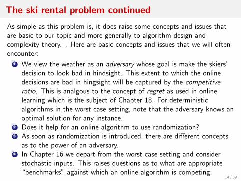
As simple as this problem is, it does raise some concepts and issues thatare basic to our topic and more generally to algorithm design andcomplexity theory. . Here are basic concepts and issues that we will oftenencounter:

1 We view the weather as an adversary whose goal is make the skiers’decision to look bad in hindsight. This extent to which the onlinedecisions are bad in hingsight will be captured by the competitiveratio. This is analgous to the concept of regret as used in onlinelearning which is the subject of Chapter 18. For deterministicalgorithms in the worst case setting, note that the adversary knows anoptimal solution for any instance.

2 Does it help for an online algorithm to use randomization?3 As soon as randomization is introduced, there are different concepts

as to the power of an adversary.4 In Chapter 16 we depart from the worst case setting and consider

stochastic inputs. This raises questions as to what are appropriate“benchmarks” against which an online algorithm is competing.

14 / 39

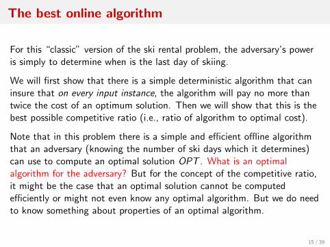
The best online algorithm

For this “classic” version of the ski rental problem, the adversary’s poweris simply to determine when is the last day of skiing.

We will first show that there is a simple deterministic algorithm that caninsure that on every input instance, the algorithm will pay no more thantwice the cost of an optimum solution. Then we will show that this is thebest possible competitive ratio (i.e., ratio of algorithm to optimal cost).

Note that in this problem there is a simple and efficient offline algorithmthat an adversary (knowing the number of ski days which it determines)can use to compute an optimal solution OPT . What is an optimalalgorithm for the adversary? But for the concept of the competitive ratio,it might be the case that an optimal solution cannot be computedefficiently or might not even know any optimal algorithm. But we do needto know something about properties of an optimal algorithm.

15 / 39

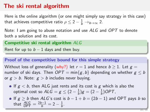
The ski rental algorithm

Here is the online algorithm (or one might simply say strategy in this case)that achieves competitive ratio ρ ≤ 2− 1

b →b→∞ 2.

Note: I am going to abuse notation and use ALG and OPT to denoteboth a solution and its cost.

Competitive ski rental algorithm ALG

Rent for up to b − 1 days and then buy.

Proof of the competitive bound for this simple strategy

Without loss of generality (why?) let r = 1 and hence b ≥ 1. Let g =number of ski days. Then OPT = ming , b depending on whether g ≤ bor g > b. Note: g > b includes never buying.

If g < b, then ALG just rents and its cost is g which is also theoptimal cost so ALG = g ≤ (2− 1

b )g = (2− 1b )OPT ,

If g ≥ b then ALG ’s cost is b − 1 + b = (2b − 1) and OPT pays b sothat ALG

OPT = 2b−1b = 2− 1

b .16 / 39

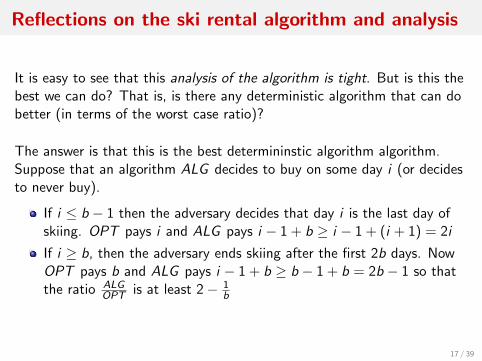
Reflections on the ski rental algorithm and analysis

It is easy to see that this analysis of the algorithm is tight. But is this thebest we can do? That is, is there any deterministic algorithm that can dobetter (in terms of the worst case ratio)?

The answer is that this is the best determininstic algorithm algorithm.Suppose that an algorithm ALG decides to buy on some day i (or decidesto never buy).

If i ≤ b − 1 then the adversary decides that day i is the last day ofskiing. OPT pays i and ALG pays i − 1 + b ≥ i − 1 + (i + 1) = 2i

If i ≥ b, then the adversary ends skiing after the first 2b days. NowOPT pays b and ALG pays i − 1 + b ≥ b − 1 + b = 2b − 1 so thatthe ratio ALG

OPT is at least 2− 1b

17 / 39

More reflections on the analysis

In principle, in competitive analysis we need not care if the onlinealgorithm is efficient. Note that is the above analysis we didn’t care howthe algorithm decided to chose i . We are just trying to uderstand thelimitations imposed by the myopic online requirement. Of course, inpractice, we do care about efficient algorithms and although the analysismay ignore computational efficiency, online algorithms tend to be veryefficient. The negative result is an example of an information theroreticargument.

Indeed the competitive ski rental algorithm is exceptionally computationalsimple. The algorithm only needs to have memory to remember what dayit is. However, we allow online algorithms to keep as much informationabout previous inputs as it wishes and make decisions based on all thisinformation.

In the analysis it seems like the adversary has to be observing what ALG isdoing to know when to end the skiing. But since ALG is deterministic, theadversary knows in advance which day (if ever) ALG will buy.

18 / 39

Can randomization help?

In a randomized online algorithm, the algorithm can make decisions as aprobabilistic function of all the previous information. Can randomizationhelp?

The answer is yes but the algorithm and its analysis is a little moreinvolved. Essentially the algorithm uses a partitcular probability densityfunction to choose the time to buy. We also have to be a little careful inwhat we mean by the competitve ratio of a randomized algorithm. But fornow here is the statement of the result (which also holds for thegeneralizations of ski rental previously mentioned):

Randomized ski rental competitive ratio

There is a randomized algorithm for the ski rental problem achievingcompetitive ratio e

e−1 ≈ 1.58 against an oblivious adversary (i.e., anadversary that see the algorithm but not the random bits and hence notthe actual decisions of the algorithm).

19 / 39

Can randomization help?

In a randomized online algorithm, the algorithm can make decisions as aprobabilistic function of all the previous information. Can randomizationhelp?The answer is yes but the algorithm and its analysis is a little moreinvolved. Essentially the algorithm uses a partitcular probability densityfunction to choose the time to buy. We also have to be a little careful inwhat we mean by the competitve ratio of a randomized algorithm. But fornow here is the statement of the result (which also holds for thegeneralizations of ski rental previously mentioned):

Randomized ski rental competitive ratio

There is a randomized algorithm for the ski rental problem achievingcompetitive ratio e

e−1 ≈ 1.58 against an oblivious adversary (i.e., anadversary that see the algorithm but not the random bits and hence notthe actual decisions of the algorithm).

19 / 39

Graham’s online and LPT makespan algorithms

Let’s continue with two greedy algorithms that date back to 1966 and1969 papers.

These are also good starting points since (precedingNP-completeness) Graham conjectured that makspan is a hard(requiring exponential time) problem to compute optimally but forwhich there were worst case approximation ratios (although he didn’tuse that terminology).

This might then be called the start of worst case approximationalgorithms. One could also even consider this to be the start of onlinealgorithms and competitive analysis (although one usually refers to a1985 paper by Sleator and Tarjan as the seminal paper in this regard).

Moreover, there are again some general concepts to be observed inthis work and even after nearly 50 years, there are still open questionsconcerning the many variants of makespan problems.

20 / 39

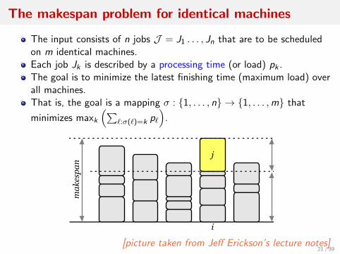
The makespan problem for identical machines

The input consists of n jobs J = J1 . . . , Jn that are to be scheduledon m identical machines.Each job Jk is described by a processing time (or load) pk .The goal is to minimize the latest finishing time (maximum load) overall machines.That is, the goal is a mapping σ : 1, . . . , n → 1, . . . ,m that

minimizes maxk

(∑`:σ(`)=k p`

).

Algorithms Lecture 30: Approximation Algorithms [Fa’10]

Theorem 1. The makespan of the assignment computed by GREEDYLOADBALANCE is at most twice themakespan of the optimal assignment.

Proof: Fix an arbitrary input, and let OPT denote the makespan of its optimal assignment. Theapproximation bound follows from two trivial observations. First, the makespan of any assignment (andtherefore of the optimal assignment) is at least the duration of the longest job. Second, the makespan ofany assignment is at least the total duration of all the jobs divided by the number of machines.

OPT≥maxj

T[ j] and OPT≥ 1

m

nj=1

T[ j]

Now consider the assignment computed by GREEDYLOADBALANCE. Suppose machine i has the largesttotal running time, and let j be the last job assigned to machine i. Our first trivial observation impliesthat T[ j] ≤ OPT. To finish the proof, we must show that Total[i]− T[ j] ≤ OPT. Job j was assignedto machine i because it had the smallest finishing time, so Total[i]− T[ j] ≤ Total[k] for all k. (Somevalues Total[k] may have increased since job j was assigned, but that only helps us.) In particular,Total[i]− T[ j] is less than or equal to the average finishing time over all machines. Thus,

Total[i]− T[ j]≤ 1

m

mi=1

Total[i] =1

m

nj=1

T[ j]≤ OPT

by our second trivial observation. We conclude that the makespan Total[i] is at most 2 ·OPT.

j ! OPT

! OPT

i

ma

kes

pa

n

Proof that GREEDYLOADBALANCE is a 2-approximation algorithm

GREEDYLOADBALANCE is an online algorithm: It assigns jobs to machines in the order that the jobsappear in the input array. Online approximation algorithms are useful in settings where inputs arrivein a stream of unknown length—for example, real jobs arriving at a real scheduling algorithm. In thisonline setting, it may be impossible to compute an optimum solution, even in cases where the offlineproblem (where all inputs are known in advance) can be solved in polynomial time. The study of onlinealgorithms could easily fill an entire one-semester course (alas, not this one).

In our original offline setting, we can improve the approximation factor by sorting the jobs beforepiping them through the greedy algorithm.

SORTEDGREEDYLOADBALANCE(T[1 .. n], m):sort T in decreasing orderreturn GREEDYLOADBALANCE(T, m)

Theorem 2. The makespan of the assignment computed by SORTEDGREEDYLOADBALANCE is at most 3/2times the makespan of the optimal assignment.

2

[picture taken from Jeff Erickson’s lecture notes]21 / 39

Aside: The Many Variants of Online Algorithms

As I indicated, Graham’s algorithm could be viewed as the first example ofwhat has become known as competitive analysis (as named in a paper byManasse, McGeoch and Sleator) following the paper by Sleator and Tarjanwhich explicitly advocated for this type of analysis. Another early (preSleator and Tarjan) example of such analysis was Yao’s analysis of onlinebin packing algorithms.

As we already stated, in competitive analysis we compare the performanceof an online algorithm against that of an optimal solution. The meaning ofonline algorithm here is that input items arrive sequentially and thealgorithm must make an irrevocable decision concerning each item. (Formakespan, an item is a job and the decision is to choose a machine onwhich the item is scheduled.)Let’s review and expand upon what we already mentioned in regard to theski rental problem.

What determines the order of input item arrivals?22 / 39

The Many Variants of Online Algorithms continued

In the “standard” meaning of online algorithms (for CS theory), wethink of an adversary as creating a nemesis input set and the orderingof the input items in that set. So this is traditional worst case analysisas in approximation algorithms applied to online algorithms. If nototherwise stated, we will assume this as the meaning of an onlinealgorithm and if we need to be more precise we can say onlineadversarial model.We will also sometimes consider an online stochastic model where anadversary defines an input distribution and then input items aresequentially generated. There can be more general stochastic models(e.g., a Markov process) but the i.i.d model is common in analysis.Stochastic analysis as often seen in OR.In the i.i.d model, we can assume that the distribution is known bythe algorithm or unknown.In the random order model (ROM), an adversary creates a size nnemesis input set and then the items from that set are given in auniform random order (i.e. uniform over the n! permutations)

23 / 39

Second aside: more general online frameworks

In the standard online model (and the variants we just mentioned), we areconsidering a one pass algorithm that makes one irrevocable decision foreach input item.

There are many extensions of this one pass paradigm. For example:

An algorithm is allowed some limited ability to revoke previousdecisions.There may be some forms of lookahead (e.g. buffering of inputs).The algorithm may maintain a “small’ number of solutions and then(say) take the best of the final solutions.The algorithm may do several passes over the input items.The algorithm may be given (in advance) some advice bits based onthe entire input.

Throughout our discussion of algorithms, we can consider deterministic orrandomized algorithms. In the online models, the randomization is interms of the decisions being made. (Of course, the ROM model is anexample of where the ordering of the inputs is randomized.)

24 / 39

A third aside: other measures of performance

The above variants address the issues of alternative input models, andrelaxed versions of the online paradigm.

Competitive analysis is really just asymptotic approximation ratio analysisapplied to online algorithms. Given the number of papers devoted toonline competitive analysis, it is the standard measure of performance.

However, it has long been recognized that as a measure of performance,competitive analysis is often at odds with what seems to be observable inpractice. Therefore, many alternative measures have been proposed. Anoverview of a more systematic study of alternative measures (as well asrelaxed versions of the online paradigm and restricted input instances) foronline algorithms is provided in Kim Larsen’s lecture slides that I haveplaced on the course web site.

See, for example, the discussion of the accommodating function measure(for the dual bin packing problem), the relative worst order meaure for thebin packing coloring problem, and the page fault rate measure for paging.

25 / 39

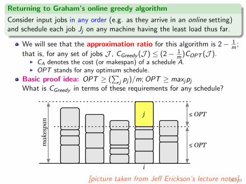
Returning to Graham’s online greedy algorithm

Consider input jobs in any order (e.g. as they arrive in an online setting)and schedule each job Jj on any machine having the least load thus far.

We will see that the approximation ratio for this algorithm is 2− 1m ;

that is, for any set of jobs J , CGreedy (J ) ≤ (2− 1m )COPT (J ).

I CA denotes the cost (or makespan) of a schedule A.I OPT stands for any optimum schedule.

Basic proof idea: OPT ≥ (∑

j pj)/m;OPT ≥ maxjpjWhat is CGreedy in terms of these requirements for any schedule?

Algorithms Lecture 30: Approximation Algorithms [Fa’10]

Theorem 1. The makespan of the assignment computed by GREEDYLOADBALANCE is at most twice themakespan of the optimal assignment.

Proof: Fix an arbitrary input, and let OPT denote the makespan of its optimal assignment. Theapproximation bound follows from two trivial observations. First, the makespan of any assignment (andtherefore of the optimal assignment) is at least the duration of the longest job. Second, the makespan ofany assignment is at least the total duration of all the jobs divided by the number of machines.

OPT≥maxj

T[ j] and OPT≥ 1

m

nj=1

T[ j]

Now consider the assignment computed by GREEDYLOADBALANCE. Suppose machine i has the largesttotal running time, and let j be the last job assigned to machine i. Our first trivial observation impliesthat T[ j] ≤ OPT. To finish the proof, we must show that Total[i]− T[ j] ≤ OPT. Job j was assignedto machine i because it had the smallest finishing time, so Total[i]− T[ j] ≤ Total[k] for all k. (Somevalues Total[k] may have increased since job j was assigned, but that only helps us.) In particular,Total[i]− T[ j] is less than or equal to the average finishing time over all machines. Thus,

Total[i]− T[ j]≤ 1

m

mi=1

Total[i] =1

m

nj=1

T[ j]≤ OPT

by our second trivial observation. We conclude that the makespan Total[i] is at most 2 ·OPT.

j ! OPT

! OPT

i

ma

kes

pa

n

Proof that GREEDYLOADBALANCE is a 2-approximation algorithm

GREEDYLOADBALANCE is an online algorithm: It assigns jobs to machines in the order that the jobsappear in the input array. Online approximation algorithms are useful in settings where inputs arrivein a stream of unknown length—for example, real jobs arriving at a real scheduling algorithm. In thisonline setting, it may be impossible to compute an optimum solution, even in cases where the offlineproblem (where all inputs are known in advance) can be solved in polynomial time. The study of onlinealgorithms could easily fill an entire one-semester course (alas, not this one).

In our original offline setting, we can improve the approximation factor by sorting the jobs beforepiping them through the greedy algorithm.

SORTEDGREEDYLOADBALANCE(T[1 .. n], m):sort T in decreasing orderreturn GREEDYLOADBALANCE(T, m)

Theorem 2. The makespan of the assignment computed by SORTEDGREEDYLOADBALANCE is at most 3/2times the makespan of the optimal assignment.

2

[picture taken from Jeff Erickson’s lecture notes]26 / 39

Graham’s online greedy algorithm

Consider input jobs in any order (e.g. as they arrive in an online setting)and schedule each job Jj on any machine having the least load thus far.

In the online “competitive analysis” literature the ratio CACOPT

is calledthe competitive ratio and it allows for this ratio to just hold in thelimit as COPT increases. This is the analogy of asymptoticapproximation ratios.

NOTE: Often, we will not provide proofs in the lecture notes but ratherwill do or sketch proofs in class (or leave a proof as an exercise).

The approximation ratio for the online greedy is “tight” in that thereis a sequence of jobs forcing this ratio.

This bad input sequence suggests a better algorithm, namely the LPT(offline or sometimes called semi-online) algorithm.

27 / 39

Graham’s LPT algorithm

Sort the jobs so that p1 ≥ p2 . . . ≥ pn and then greedily schedule jobs onthe least loaded machine.

The (tight) approximation ratio of LPT is(43 −

13m

).

It is believed that this is the best “greedy” algorithm but how wouldone prove such a result? This of course raises the question as to whatis a greedy algorithm.

We will present the priority model for greedy (and greedy-like)algorithms. I claim that all the algorithms mentioned on slide 10 canbe formulated within the priority model.

Assuming we maintain a priority queue for the least loaded machine,I the online greedy algorithm would have time complexity O(n logm)

which is (n log n) since we can assume n ≥ m.I the LPT algorithm would have time complexity O(n log n).

28 / 39

Partial Enumeration Greedy

Combining the LPT idea with a brute force approach improves theapproximation ratio but at a significant increase in time complexity.

I call such an algorithm a “partial enumeration greedy” algorithm.

Optimally schedule the largest k jobs (for 0 ≤ k ≤ n) and then greedilyschedule the remaining jobs (in any order).

The algorithm has approximation ratio no worse than

(1 +

1− 1m

1+bk/mc

).

Graham also shows that this bound is tight for k ≡ 0 mod m.

The running time is O(mk + n log n).

Setting k = 1−εε m gives a ratio of at most (1 + ε) so that for any

fixed m, this is a PTAS (polynomial time approximation scheme).with time O(mm/ε + n log n).

29 / 39

Makespan: Some additional comments

There are many refinements and variants of the makespan problem.

There was significant interest in the best competitive ratio (in theonline setting) that can be achieved for the identical machinesmakespan problem.

The online greedy gives the best online ratio for m = 2,3 but betterbounds are known for m ≥ 4. For arbitrary m, as far as I know,following a series of previous results, the best known approximationratio is 1.9201 (Fleischer and Wahl) and there is 1.88 inapproximationbound (Rudin). Basic idea: leave some room for a possible large job;this forces the online algorithm to be non-greedy in some sense butstill within the online model.

Randomization can provide somewhat better competitive ratios.

Makespan has been actively studied with respect to three othermachine models.We plan to consider these other models when we get to Chapter 4.

30 / 39

The uniformly related machine model

Each machine i has a speed si

As in the identical machines model, job Jj is described by aprocessing time or load pj .

The processing time to schedule job Jj on machine i is pj/si .

There is an online algorithm that achieves a constant competitiveratio.

I think the best known deterministic (resp. randomized) online ratio is5.828 (resp. 4.311) due to P. Berman et al [2000] following the firstconstant ratio by Aspnes et al.

Ebenlendr and Sgall [2015] establish a deterministic onlineinapproximation of 2.564 following the 2.438 deterministic onlineinapproximation of Berman et al. who also proved a 1.8372inapproximation for any randomized online algorithm.

31 / 39

The restricted machines model

Every job Jj is described by a pair (pj , Sj) where Sj ⊆ 1, . . . ,m isthe set of machines on which Jj can be scheduled.This (and the next model) have been the focus of a number of papers(for both online and offline) and there has been some relatively recentprogress in the offline restricted machines case.Even for the case of two allowable machines per job (i.e. the graphorientation problem), this is an interesting problem and we will lookat some recent work later.Azar et al show that log2(m) (resp. ln(m)) is (up to ±1) the bestcompetitive ratio for deterministic (resp. randomized) onlinealgorithms with the upper bounds obtained by the “natural greedyalgorithm”.It is not known if there is an offline greedy-like algorithm for thisproblem that achieves a constant approximation ratio. Regev [IPL2002] shows an Ω( logm

log logm ) inapproximation for “fixed order priorityalgorithms” for the restricted case when every job has 2 allowablemachines.

32 / 39

The unrelated machines model

This is the most general of the makespan machine models.

Now a job Jj is represented by a vector (pj ,1, . . . , pj ,m) where pj ,i isthe time to process job Jj on machine i .

A classic result of Lenstra, Shmoys and Tardos [1990] shows how tosolve the (offline) makespan problem in the unrelated machine modelwith approximation ratio 2 using LP rounding.

There is an online algorithm with approximation O(logm). Currently,this is the best approximation known for greedy-like (e.g. priority)algorithms even for the restricted machines model although there hasbeen some progress made in this regard (which we will discuss later).

NOTE: All statements about what we will do later should beunderstood as intentions and not promises.

33 / 39

Makespan with precedence constraints; how muchshould we trust our intuition

Graham also considered the makespan problem on identical machines forjobs satisfying a precedence constraint. Suppose ≺ is a partial ordering onjobs meaning that if Ji ≺ Jk then Ji must complete before Jk can bestarted. Assuming jobs are ordered so as to respect the partial order (i.e.,can be reordered within the priority model) Graham showed that the ratio2− 1

m is achieved by “the natural greedy algorithm”, call it G≺.

Graham’s 1969 paper is entitled “Bounds on Multiprocessing TimingAnomalies” pointing out some very non-intuitive anomalies that can occur.

Consider G≺ and suppose we have a given an input instance of themakespan with precedence problem. Which of the following should neverlead to an increase in the makepan objective for the instance?

Relaxing the precedence ≺Decreasing the processing time of some jobsAdding more machines

In fact, all of these changes could increase the makespan value.

34 / 39

Makespan with precedence constraints; how muchshould we trust our intuition

Graham also considered the makespan problem on identical machines forjobs satisfying a precedence constraint. Suppose ≺ is a partial ordering onjobs meaning that if Ji ≺ Jk then Ji must complete before Jk can bestarted. Assuming jobs are ordered so as to respect the partial order (i.e.,can be reordered within the priority model) Graham showed that the ratio2− 1

m is achieved by “the natural greedy algorithm”, call it G≺.

Graham’s 1969 paper is entitled “Bounds on Multiprocessing TimingAnomalies” pointing out some very non-intuitive anomalies that can occur.

Consider G≺ and suppose we have a given an input instance of themakespan with precedence problem. Which of the following should neverlead to an increase in the makepan objective for the instance?

Relaxing the precedence ≺Decreasing the processing time of some jobsAdding more machines

In fact, all of these changes could increase the makespan value. 34 / 39

The bin packing problem

Our next classic minimization problem is the one-dimensional bin packingproblem. In this problem we have a set of items each having a size orweight xj and these items have to all be packed into bins of a fixed size B.The objective is to minimize the number of bins. (This problem issometimes referred to as the cutting stock problem). Without loss ofgenerality, we can set B = 1 and then assume that xj ≤ 1 for all j .

Online bin packing was first studied in a 1972 STOC conference paper byGarey, Graham and Ullman, and then in a 1973 Johnson FOCS paper, andin a 1974 journal article combining Garey et al with David Johnson andAlan Demers. There are many subsequent bin packing papers dealing withonline and greedy type algorithms. This work (proceeded by Graham’searlier makespan results) became the driving force for the area ofapproximation algiorithms following the introduction of NP-completeness.Johnson’s PHD thesis was devoted to approximation algorithms.

35 / 39

Bin packing continued

There are some natural online algorithms for the bin packing problemwhich in turn have natural greedy extensions when initially ordering the xj .Furthermore, although the problem is also NP-complete, (i.e., deciding ifan instance can be packed into 2 bins is NP complete), there are offlinealgorithms ALG such that ALG ≤ OPT + o(OPT ) so that the asymptoticapproximation ratio is 1. As far as I know, as an offline problem there maybe an algorithm that achieves ALG ≤ OPT + 1.

There are also higher dimensional versions. For example, in dimension 2,the goal is to pack rectangles (usually axis aligned) into say 1 by 1 squarebins.

36 / 39

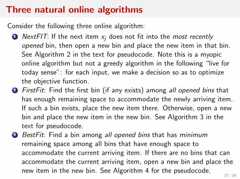
Three natural online algorithms

Consider the following three online algorithm:

1 NextFIT: If the next item xj does not fit into the most recentlyopened bin, then open a new bin and place the new item in that bin.See Algorithm 2 in the text for pseudocode. Note this is a myopiconline algorithm but not a greedy algorithm in the following “live fortoday sense”: for each input, we make a decision so as to optimizethe objective function.

2 FirstFit: Find the first bin (if any exists) among all opened bins thathas enough remaining space to accommodate the newly arriving item.If such a bin exists, place the new item there. Otherwise, open a newbin and place the new item in the new bin. See Algorithm 3 in thetext for pseudocode.

3 BestFit: Find a bin among all opened bins that has minimumremaining space among all bins that have enough space toaccommodate the current arriving item. If there are no bins that canaccommodate the current arriving item, open a new bin and place thenew item in the new bin. See Algorithm 4 for the pseudocode.

37 / 39

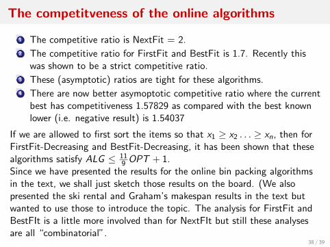
The competitveness of the online algorithms

1 The competitive ratio is NextFit = 2.2 The competitive ratio for FirstFit and BestFit is 1.7. Recently this

was shown to be a strict competitive ratio.3 These (asymptotic) ratios are tight for these algorithms.4 There are now better asymoptotic competitive ratio where the current

best has competitiveness 1.57829 as compared with the best knownlower (i.e. negative result) is 1.54037

If we are allowed to first sort the items so that x1 ≥ x2 . . . ≥ xn, then forFirstFit-Decreasing and BestFit-Decreasing, it has been shown that thesealgorithms satisfy ALG ≤ 11

9 OPT + 1.Since we have presented the results for the online bin packing algorithmsin the text, we shall just sketch those results on the board. (We alsopresented the ski rental and Graham’s makespan results in the text butwanted to use those to introduce the topic. The analysis for FirstFit andBestFIt is a little more involved than for NextFIt but still these analysesare all “combinatorial”.

38 / 39

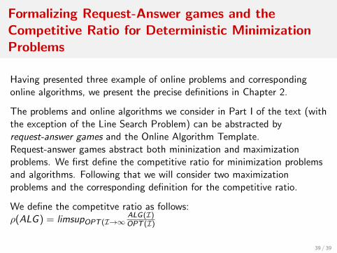
Formalizing Request-Answer games and theCompetitive Ratio for Deterministic MinimizationProblems

Having presented three example of online problems and correspondingonline algorithms, we present the precise definitions in Chapter 2.

The problems and online algorithms we consider in Part I of the text (withthe exception of the Line Search Problem) can be abstracted byrequest-answer games and the Online Algorithm Template.Request-answer games abstract both mininization and maximizationproblems. We first define the competitive ratio for minimization problemsand algorithms. Following that we will consider two maximizationproblems and the corresponding definition for the competitive ratio.

We define the competitve ratio as follows:ρ(ALG ) = limsupOPT (I→∞

ALG(I)OPT (I)

39 / 39

csc2421 topics in algorithms: online and other myopic

Documents