1

CS 512 Machine Learning

Berrin YanikogluSlides are expanded from the Machine Learning-Mitchell book slidesSome of the extra slides thanks to T. Jaakkola, MIT and others

2

CS512-Machine Learning Please refer to http://people.sabanciuniv.edu/berrin/cs512/

for course information. This webpage is also linked from SuCourse.

We will use SuCourse mainly for assignments and announcements. You are responsible of checking SuCourse for announcements.

Undergraduates are required to attend the course; graduates are strongly encouraged to.

3

Important Info

Grading: 2 midterms for a total of 50%; In-class final: 25%; Homeworks: 15% Group project: 10%;

Missed Exams: You can miss up to one midterm (no proof is required), in which case the weight

of the final will increase (to 50%). If you miss two midterms, you get an F. To encourage exam participation, some brownie points will be given to those who

attend both midterm exams (otherwise those taking a good grade in Mt1 does not attend Mt2). I do consider Mt attendance if someone is at the border of a grade cluster.

If you miss the final exam, you MUST have a legitimate excuse/report.

Passing Grade: To pass the course you grade as calculated above must be at least 35 (strict)

and Final grade should be above 30/100.

What is Learning...

5

What is learning?It is very difficult to pin down what learning is. As our programs/agents/robots start doing more and more things, we do not find them intelligent anymore.

Some definitions from famous people in CS/AI history: “Learning denotes changes in a system that ... enable a

system to do the same task more efficiently the next time.” –Herbert Simon

“Learning is any process by which a system improves performance from experience.” –Herbert Simon

“Learning is constructing or modifying representations of what is being experienced.” –Ryszard Michalski

“Learning is making useful changes in our minds.” –Marvin Minsky

6

7

Why learn?

Build software agents that can adapt to their users or to other software agents or to changing environments Mars robot

Develop systems that are too difficult/expensive to construct manually because they require specific detailed skills or knowledge tuned to a specific task Large, complex AI systems cannot be completely

derived by hand and require dynamic updating to incorporate new information.

Discover new things that were previously unknown to humans Examples: data mining, scientific discovery

8

9

Related Disciplines

The following are close disciplines: Artificial Intelligence

Machine learning deals with the learning part of AI Pattern Recognition

Concentrates more on “tools” rather than theory Data Mining

More specific about discovery

The following are useful in machine learning techniques or may give insights: Probability and Statistics Information theory

Psychology (developmental, cognitive) Neurobiology Linguistics Philosophy

10

History of Machine Learning

1950s Samuel’s checker player Selfridge’s Pandemonium

1960s: Neural networks: Perceptron Minsky and Papert prove limitations of Perceptron

1970s: Expert systems and the knowledge acquisition bottleneck Mathematical discovery with AM Symbolic concept induction Winston’s arch learner Quinlan’s ID3 Michalski’s AQ and soybean diagnosis Scientific discovery with BACON

11

History of Machine Learning (cont.) 1980s:

Resurgence of neural networks (connectionism, backpropagation)

Advanced decision tree and rule learning Explanation-based Learning (EBL) Learning, planning and problem solving Utility theory Analogy Cognitive architectures Valiant’s PAC Learning Theory

1990s Data mining Reinforcement learning (RL) Inductive Logic Programming (ILP) Ensembles: Bagging, Boosting, and Stacking

12

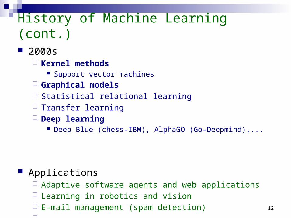
History of Machine Learning (cont.)

2000s Kernel methods

Support vector machines Graphical models Statistical relational learning Transfer learning Deep learning

Deep Blue (chess-IBM), AlphaGO (Go-Deepmind),...

Applications Adaptive software agents and web applications Learning in robotics and vision E-mail management (spam detection) …

Different Learning Paradigms

14

Major paradigms of machine learning

Rote learning – “Learning by memorization.” Employed by first machine learning systems, in 1950s

Samuel’s Checkers program

Supervised learning – Use specific examples to reach general conclusions or extract general rules

Classification (Concept learning) Regression

Unsupervised learning (Clustering) – Unsupervised identification of natural groups in data

Reinforcement learning– Feedback (positive or negative reward) given at the end of a sequence of steps

Analogy – Determine correspondence between two different representations

Discovery – Unsupervised, specific goal not given

15

Rote Learning is Limited

Memorize I/O pairs and perform exact matching with new inputs

If a computer has not seen the precise case before, it cannot apply its experience

We want computers to “generalize” from prior experience Generalization is the most important factor in learning

16

The inductive learning problem Extrapolate from a given set of examples to make

accurate predictions about future examples

Supervised versus unsupervised learning Learn an unknown function f(X) = Y, where X is an input

example and Y is the desired output. Supervised learning implies we are given a training set of

(X, Y) pairs by a “teacher” Unsupervised learning means we are only given the Xs. Semi-supervised learning: mostly unlabelled data

Classification, Regression

18

Types of supervised learning

x1=size

x2=color

Tangerines Oranges

a) Classification: • We are given the label of the training

objects: {(x1,x2,y=T/O)}

• We are interested in classifying future objects: (x1’,x2’) with the correct label.

I.e. Find y’ for given (x1’,x2’).

b) Concept Learning:

• We are given positive and negative samples for the concept we want to learn (e.g.Tangerine): {(x1,x2,y=+/-)}

• We are interested in classifying future

objects as member of the class (or positive example for the concept) or not.

I.e. Answer +/- for given (x1’,x2’).

19

Types of Supervised Learning Regression

Target function is continuous rather than class membership

For example, you have some the selling prices of houses as their sizes (sq-mt) changes in a particular location that may look like this. You may hypothesize that the prices are governed by a particular function f(x). Once you have this function that “explains” this relationship, you can guess a given house’s value, given its sq-mt. The learning here is the selection of this function f() .

Note that the problem is more meaningful and challenging if you imagine several input parameters, resulting in a multi-dimensional input space.

60 70 90 120 150 x=size

y=price

f(x)

20

Classification

Assign object/event to one of a given finite set of categories. Medical diagnosis Credit card applications or transactions Fraud detection in e-commerce Spam filtering in email Recommended books, movies, music Financial investments Spoken words Handwritten letters

21

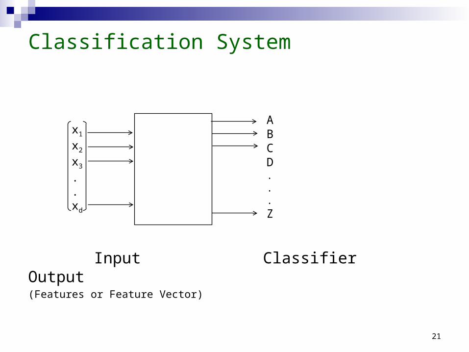
Classification System

Input Classifier Output(Features or Feature Vector)

ABCD...Z

x1

x2

x3

.

.xd

22

Regression System

Input Classifier Output(Features or Feature Vector)

f(x1, x2, x3, ..., xd)

x1

x2

x3

.

.xd

Learning: Key steps

Now that we have learned the the main supervised learning paradigms and the beginning terminology, let us look at the learning problem in a bit more detail.

24

Learning: Key Steps• data and assumptions

– what data is available for the learning task?– what can we assume about the problem?

• representation– how should we represent the examples to be classified

• method and estimation– what are the possible hypotheses?– what learning algorithm to use to infer the most likely hypothesis?

• evaluation– how well are we doing?

…

25

26

27

28

29

30

Evaluation of Learning Systems

Experimental Conduct controlled cross-validation experiments to compare

various methods on a variety of benchmark datasets. Gather data on their performance, e.g. test accuracy,

training-time, testing-time… Maybe even analyze differences for statistical significance.

Theoretical Analyze algorithms mathematically and prove theorems about

their: Ability to fit training data Computational complexity Sample complexity (number of training examples needed to learn an

accurate function)

31

Measuring Performance

Performance of the learner can be measured in one of the following ways, as suitable for the application: Accuracy

Number of mistakes (in classification problems)

Mean Squared Error (in regression problems)

Loss functions (more general, taking into account different costs for different mistakes)

Solution quality (length, efficiency) Speed of performance …

32

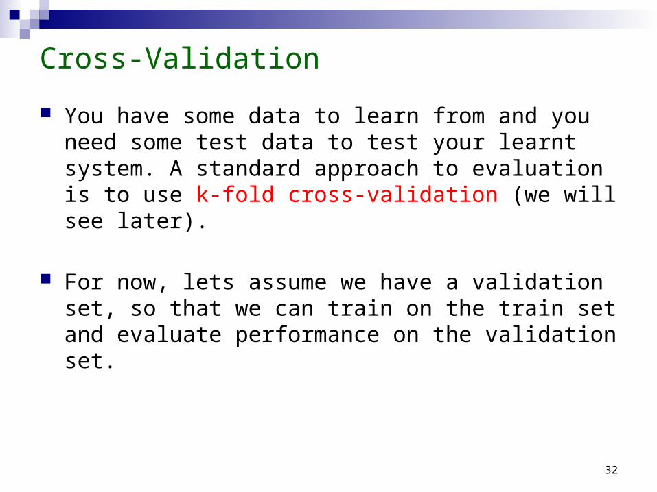
Cross-Validation

You have some data to learn from and you need some test data to test your learnt system. A standard approach to evaluation is to use k-fold cross-validation (we will see later).

For now, lets assume we have a validation set, so that we can train on the train set and evaluate performance on the validation set.

33

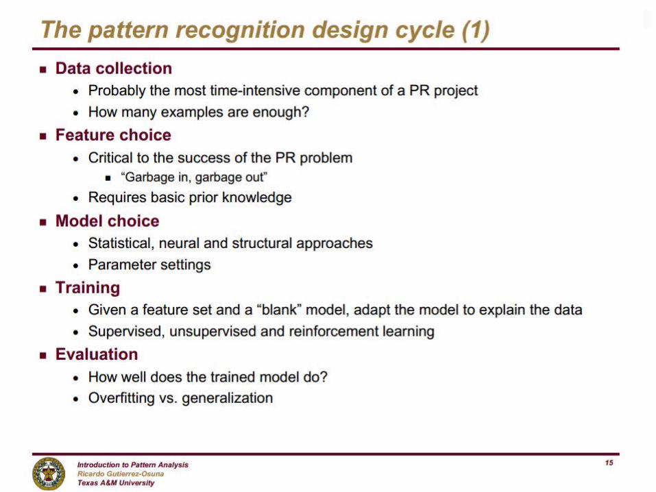
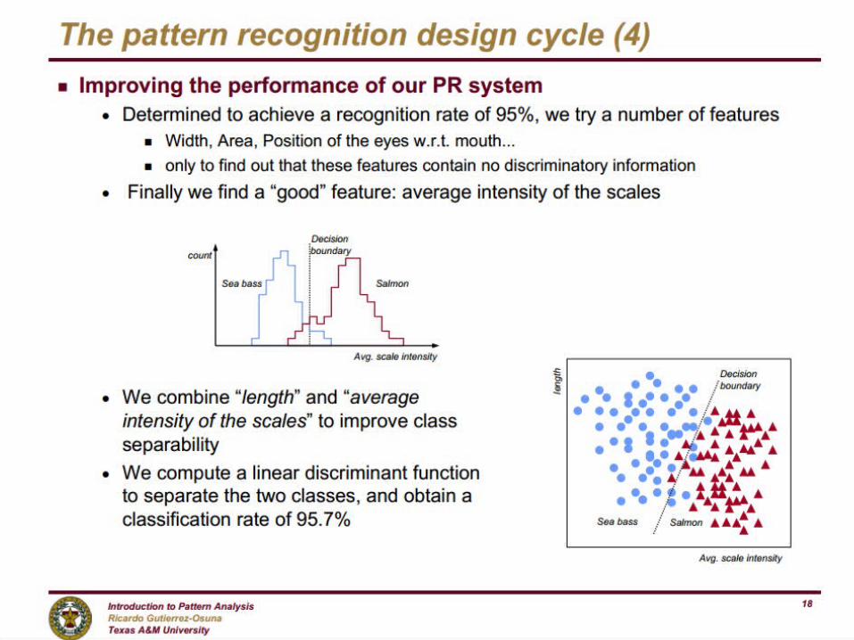
The next slides review the design cycle as a whole processfrom Gutierrez-Osuna, Texas A&M

34

35

36

37

38

39

40

Generalization and over-fitting are at the core of machine learning

Introduction to Overfitting

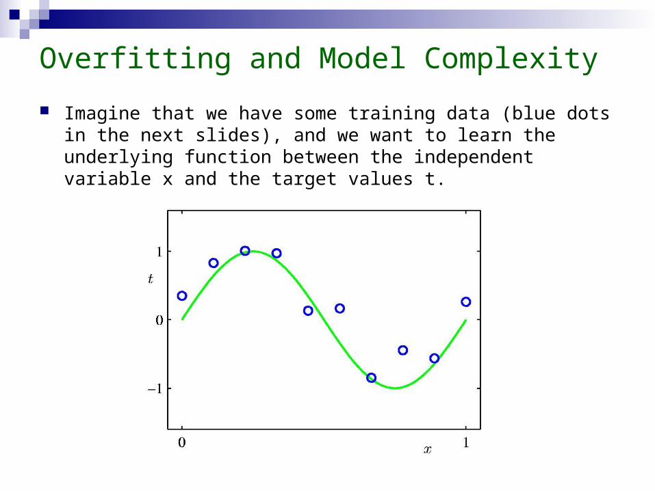
Overfitting and Model Complexity

Imagine that we have some training data (blue dots in the next slides), and we want to learn the underlying function between the independent variable x and the target values t.

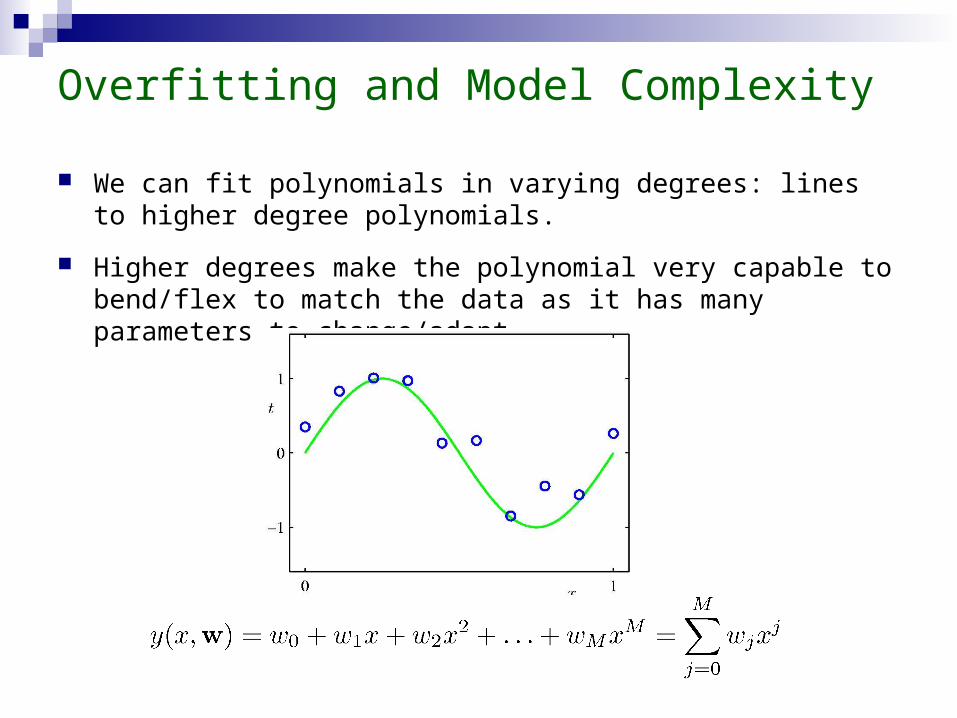
Overfitting and Model Complexity

We can fit polynomials in varying degrees: lines to higher degree polynomials.

Higher degrees make the polynomial very capable to bend/flex to match the data as it has many parameters to change/adapt.

Polynomial Curve Fitting

Overfitting and Model Complexity

We can fit polynomials in varying degrees: lines to higher degree polynomials.

Higher degrees make the polynomial very capable to bend/flex to match the data as it has many parameters to change/adapt.

Sum-of-Squares Error Function

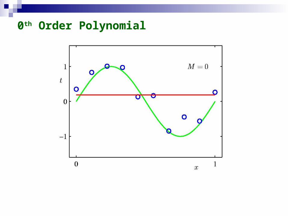
0th Order Polynomial

1st Order Polynomial

3rd Order Polynomial

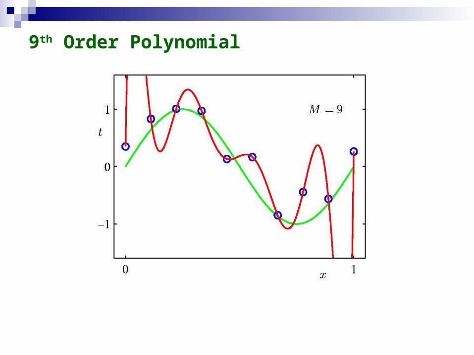
9th Order Polynomial

We do not know yet which is the best model, maybe the 9th degree polynomial after all.

52

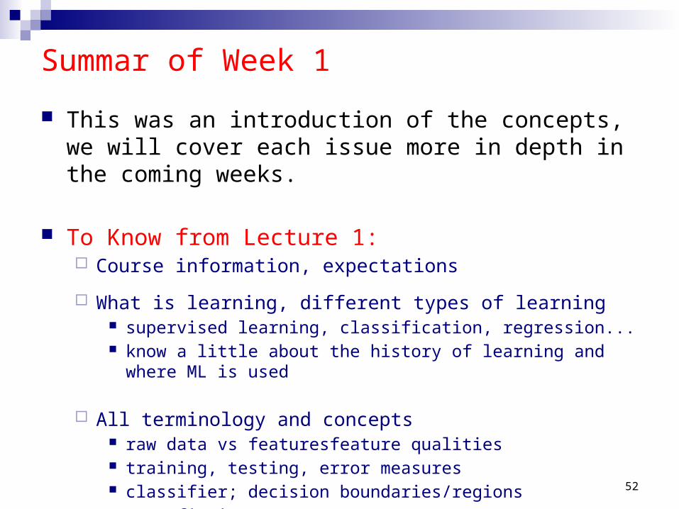
Summar of Week 1

This was an introduction of the concepts, we will cover each issue more in depth in the coming weeks.

To Know from Lecture 1: Course information, expectations

What is learning, different types of learning supervised learning, classification, regression... know a little about the history of learning and where ML is used

All terminology and concepts raw data vs featuresfeature qualities training, testing, error measures classifier; decision boundaries/regions over-fitting ...