CS 394CSeptember 16, 2013

Tandy WarnowDepartment of Computer Sciences

University of Texas at Austin

Phylogeny

Orangutan Gorilla Chimpanzee Human

From the Tree of the Life Website,University of Arizona

Phylogeny Problem

TAGCCCA TAGACTT TGCACAA TGCGCTTAGGGCAT

U V W X Y

U

V W

X

Y

Possible Indo-European tree(Ringe, Warnow and Taylor 2000)

Questions about Indo-European (IE)

• How did the IE family of languages evolve?

• Where is the IE homeland?

• When did Proto-IE “end”?

• What was life like for the speakers of proto-Indo-

European (PIE)?

The Kurgan Expansion

• Date of PIE ~4000 BCE.

• Map of Indo-European migrations from ca. 4000 to 1000 BC according to the Kurgan model

• From http://indo-european.eu/wiki

The Anatolian hypothesis (from wikipedia.org)

Date for PIE ~7000 BCE

Historical Linguistic Data

• A character is a function that maps a set of languages, L, to a set of states.

• Three kinds of characters:– Phonological (sound changes)– Lexical (meanings based on a wordlist)– Morphological (especially inflectional)

Phylogenies of Languages

• Languages evolve over time, just as biological species do (geographic and other separations induce changes that over time make different dialects incomprehensible -- and new languages appear)

• The result can be modelled as a rooted tree

• The interesting thing is that many characteristics of languages evolve without back mutation or parallel evolution (i.e., homoplasy-free) -- so a “perfect phylogeny” is possible!

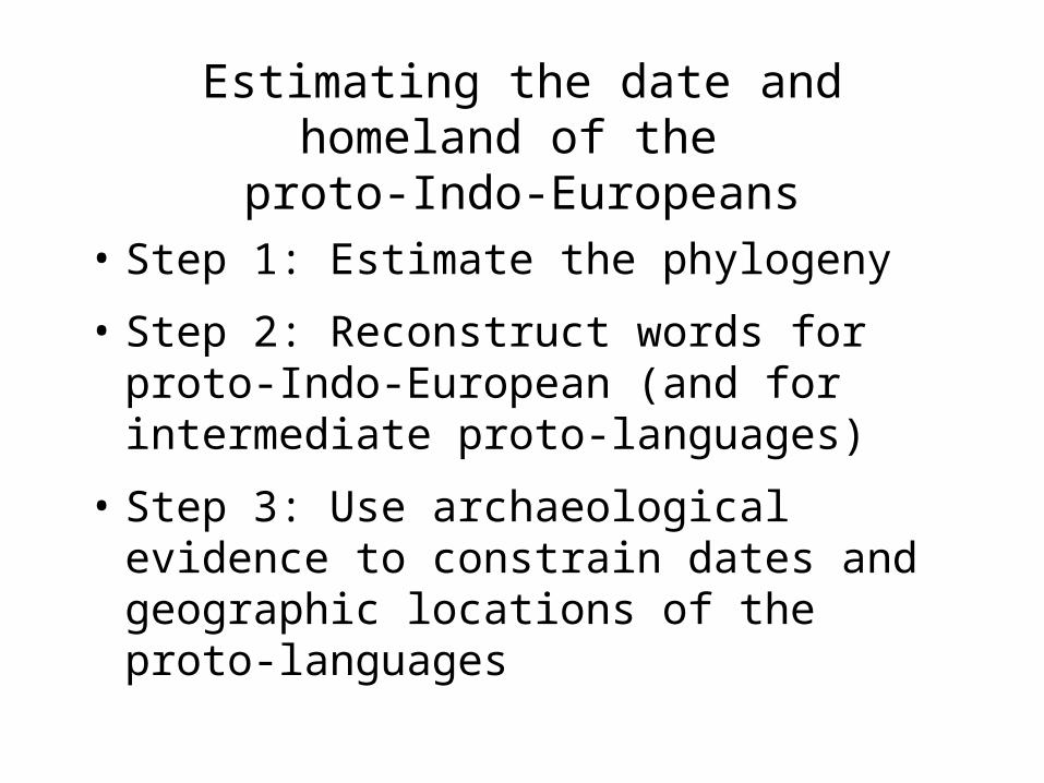
Estimating the date and homeland of the proto-Indo-Europeans

• Step 1: Estimate the phylogeny

• Step 2: Reconstruct words for proto-Indo-European (and for intermediate proto-languages)

• Step 3: Use archaeological evidence to constrain dates and geographic locations of the proto-languages

Our objectives

How to estimate the phylogeny?

How to model linguistic character evolution?

Part 1

• Triangulating colored graphs

• Perfect phylogenies

Triangulated Graphs

• Definition: A graph is triangulated if it has no simple cycles of size four or more.

Triangulated graphs and phylogeny estimation

• The “Triangulating Colored Graphs” problem and an application to historical linguistics (this talk)

• Using triangulated graphs to improve the accuracy and sequence length requirements phylogeny estimation in biology (absolute-fast converging methods)

• Using triangulated graphs to speed-up heuristics for NP-hard phylogenetic estimation problems (Rec-I-DCM3-boosting)

Some useful terminology: homoplasy

0 0 1 1

0

0

0

0 1 1 0 0

0

1

1

0 1 0 0 1

0

1

0

1

1 0 0

no homoplasy back-mutation parallel evolution

Perfect Phylogeny

• A phylogeny T for a set S of taxa is a perfect phylogeny if each state of each character occupies a subtree (no character has back-mutations or parallel evolution)

Perfect phylogenies, cont.

• A=(0,0), B=(0,1), C=(1,3), D=(1,2) has a perfect phylogeny!

• A=(0,0), B=(0,1), C=(1,0), D=(1,1) does not have a perfect phylogeny!

A perfect phylogeny

• A = 0 0

• B = 0 1

• C = 1 3

• D = 1 2

A

B

C

D

A perfect phylogeny

• A = 0 0

• B = 0 1

• C = 1 3

• D = 1 2

• E = 0 3

• F = 1 3

A

B

C

D

E F

The Perfect Phylogeny Problem

• Given a set S of taxa (species, languages, etc.) determine if a perfect phylogeny T exists for S.

• The problem of determining whether a perfect phylogeny exists is NP-hard (McMorris et al. 1994, Steel 1991).

Triangulated Graphs

• Definition: A graph is triangulated if it has no simple cycles of size four or more.

Triangulated graphs and trees

• A graph G=(V,E) is triangulated if and only if there exists a tree T so that G is the intersection graph of a set of subtrees of T.

– vertices of G correspond to subtrees (f(v) is a subtree of T)

– (v,w) is an edge in G if and only if f(v) and f(w) have a non-empty intersection

c-Triangulated Graphs

• A vertex-colored graph is c-triangulated if it is triangulated, but also properly colored!

Triangulating Colored Graphs:An Example

A graph that can be c-triangulated

Triangulating Colored Graphs:An Example

A graph that can be c-triangulated

Triangulating Colored Graphs:An Example

A graph that cannot be c-triangulated

Triangulating Colored Graphs (TCG)

Triangulating Colored Graphs: given a vertex-colored graph G, determine if G can be c-triangulated.

The PP and TCG Problems

• Buneman’s Theorem: A perfect phylogeny exists for a set S if and only if the associated character state intersection graph can be c-triangulated.

• The PP and TCG problems are polynomially equivalent and NP-hard.

A no-instance of Perfect Phylogeny

• A = 0 0

• B = 0 1

• C = 1 0

• D = 1 1

0 1

0

1

An input to perfect phylogeny (left) of four sequences describedby two characters, and its character state intersection graph. Note that the character state intersection graph is 2-colored.

Solving the PP Problem Using Buneman’s Theorem

“Yes” Instance of PP:

c1 c2 c3

s1 3 2 1

s2 1 2 2

s3 1 1 3

s4 2 1 1

Solving the PP Problem Using Buneman’s Theorem

“Yes” Instance of PP:

c1 c2 c3

s1 3 2 1

s2 1 2 2

s3 1 1 3

s4 2 1 1

Some special cases are easy

• Binary character perfect phylogeny solvable in linear time

• r-state characters solvable in polynomial time for each r (combinatorial algorithm)

• Two character perfect phylogeny solvable in polynomial time (produces 2-colored graph)

• k-character perfect phylogeny solvable in polynomial time for each k (produces k-colored graphs -- connections to Robertson-Seymour graph minor theory)

Part II

• Historical Linguistics data

• Phylogenetic tree estimation methods

• Phylogenetic network estimation methods

• Stochastic models for linguistic evolution

• Trees and Networks for Indo-European

• Comments about IE history

Possible Indo-European tree(Ringe, Warnow and Taylor 2000)

Phylogenies of Languages

• Languages evolve over time, just as biological species do (geographic and other separations induce changes that over time make different dialects incomprehensible -- and new languages appear)

• The result can be modelled as a rooted tree

• The interesting thing is that many characteristics of languages evolve without back mutation or parallel evolution -- so a “perfect phylogeny” is possible!

TAGCCCA TAGACTT TGCACAA TGCGCTTAGGGCAT

U V W X Y

U

V W

X

Y

Standard Markov models of biomolecular sequence evolution

• Sequences evolve just with substitutions

• There are a finite number of states (four for DNA and RNA, 20 for aminoacids)

• Sites (i.e., positions) evolve identically and independently, and have “rates of evolution” that are drawn from a common distribution (typically gamma)

• Numerical parameters describe the probability of substitutions of each type on each edge of the tree

Rates-across-sites

• Dates at nodes are only identifiable under rates-across-sites models with simple distributions, and also requires an approximate lexical clock.

AB

C

D

AB

C

D

Violating the rates-across-sites assumption

• The tree is fixed, but do not just scale up and down.

• Dates are not identifiable.

A

B

C

D

A BC

D

Linguistic character evolution

• Homoplasy is much less frequent: most changes result in a new state (and hence there is an unbounded number of possible states).

• The rates-across-sites assumption is unrealistic

• The lexical clock is known to be false

• Borrowing between languages occurs, but can often be detected.

These properties are very different from models for molecular sequence evolution. Phylogeny estimation requires different techniques.

Dating nodes requires both an approximate lexical clock and also the rates-across-sites assumption. Neither is likely to be true.

Historical Linguistic Data

• A character is a function that maps a set of languages, L, to a set of states.

• Three kinds of characters:– Phonological (sound changes)– Lexical (meanings based on a wordlist)– Morphological (especially inflectional)

Sound changes

• Many sound changes are natural, and should not be used for phylogenetic reconstruction.

• Others are bizarre, or are composed of a sequence of simple sound changes. These are useful for subgrouping purposes. Example: Grimm’s Law.

1. Proto-Indo-European voiceless stops change into voiceless fricatives.

2. Proto-Indo-European voiced stops become voiceless stops.

3. Proto-Indo-European voiced aspirated stops become voiced fricatives.

Homoplasy-free evolution

• When a character changes state, it changes to a new state not in the tree

• In other words, there is no homoplasy (character reversal or parallel evolution)

• First inferred for weird innovations in phonological characters and morphological characters in the 19th century, and used to establish all the major subgroups within Indo-European. 0 0 0 1 1

0

1

0

0

Lexical characters can also evolve without homoplasy

• For every cognate class, the nodes of the tree in that class should form a connected subset - as long as there is no undetected borrowing nor parallel semantic shift.

0 0 1 1 2

1

1

1

0

Phylogeny estimation

• Linguists estimate the phylogeny through intensive analysis of a relatively small amount of data

– a few hundred lexical items, plus

– a small number of morphological, grammatical, and phonological features

• All data preprocessed for homology assessment and cognate judgments

• All “homoplasy” (parallel evolution, back mutation, or borrowing) must be explained and linguistically believable

Tree estimation methods

• (weighted) Maximum Parsimony

• (weighted) Maximum Compatibility

• Neighbor-joining on distances between languages

• Analyses based upon binary-encodings of linguistic data

Methods based upon binary encoding

• Each multi-state character is split into several binary characters

• The resultant binary character matrix can be analyzed using most phylogeny estimation methods (distance-based methods, maximum parsimony, maximum compatibility, likelihood-based methods)

Binary character likelihood-based methods

• You need to specify the model (and so the probability of 0->1 and 1->0) for each binary character. For example, you may constrain 0->1 to be as likely as 1-> 0 (Cavender-Farris), or not.

• Rates-across-sites issues• Note the lack of independence between

characters.

Likelihood-based approaches

• Gray and Atkinson used a Bayesian method to estimate a distribution on trees for Indo-European, using binary encodings of lexical data.

• Others have done similar analyses on binary encodings of multi-state characters, but treated the binary matrices differently

• Other approaches have used finite-state characters, and assumed a Jukes-Cantor model for those finite states, and analyzed linguistic data.

• Many analyses are restricted to lexical characters

• Trees estimated by different groups have been quite different, in interesting ways

• IE analyses are particularly “hot” (and also “heated”)

• Our own group has proposed an infinite-states model, and showed how to calculate likelihoods efficiently under the model (but not done analyses of lexical data under the model).

Our (RWT) Data• Ringe & Taylor (2002)

– 259 lexical

– 13 morphological

– 22 phonological

• These data have cognate judgments estimated by Ringe and Taylor, and vetted by other Indo-Europeanists. (Alternate encodings were tested, and mostly did not change the reconstruction.)

• Polymorphic characters, and characters known to evolve in parallel, were removed.

First analysis: “Weighted Maximum Compatibility”

• Input: set L of languages described by characters

• Output: Tree with leaves labelled by L, such that the number of homoplasy-free (compatible) characters is maximized (while requiring that certain of the morphological and phonological characters be compatible).

• NP-hard.

The WMC Tree dates are approximate

95% of the characters are compatible

Our methods/models • Ringe & Warnow “Almost Perfect Phylogeny”: most characters evolve

without homoplasy under a no-common-mechanism assumption (various publications since 1995)

• Ringe, Warnow, & Nakhleh “Perfect Phylogenetic Network”: extends APP model to allow for borrowing, but assumes homoplasy-free evolution for all characters (Language, 2005)

• Warnow, Evans, Ringe & Nakhleh “Extended Markov model”: parameterizes PPN and allows for homoplasy provided that homoplastic states can be identified from the data. Under this model, trees and some networks are identifiable, and likelihood on a tree can be calculated in linear time (Cambridge University Press, 2006)

• Ongoing work: incorporating unidentified homoplasy and polymorphism (two or more words for a single meaning)

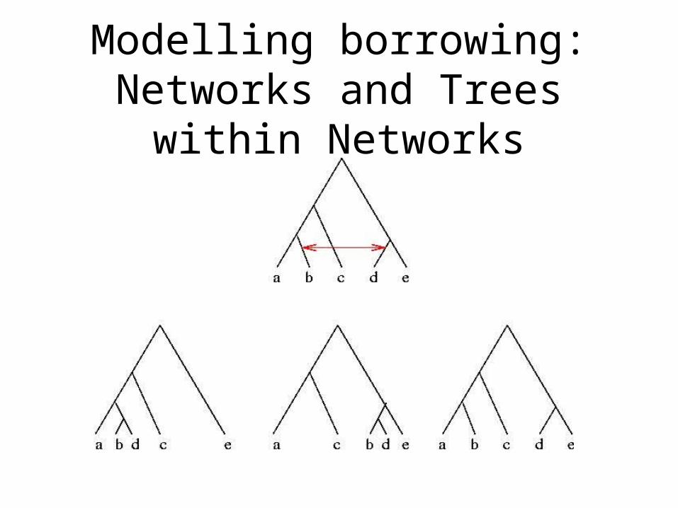
Modelling borrowing: Networks and Trees within Networks

“Perfect Phylogenetic Network” (all characters compatible)

Extended Markov model

• Each character evolves down the tree. • There are two types of states: those that can arise more

than once, and those that can only arise once. We also know which type each state is.

• Characters evolve independently but not identically, nor in a rates-across-sites fashion.

• Essentially this is a linguistic version of the no-common-mechanism model, but allowing for an infinite number of states.

Initial results

• Under very mild conditions (substitution probabilities bounded away from 1 and 0), the model tree is identifiable - even without identically distributed sites.

• Fast, statistically consistent, methods exist for reconstructing the tree (and the network, under some conditions).

• Maximum Likelihood and Bayesian analyses are also feasible, since likelihood calculations can be done in linear time.

What about PIE homeland and date?

• Linguists have “reconstructed” words for ‘wool’, ‘horse’, ‘thill’ (harness pole), and ‘yoke’, for Proto-Indo-European, and for ‘wheel’ for the ancestor of the “core” (IE minus Anatolian and Tocharian).

• Archaeological evidence (positive and negative) for these objects used to constrain the date and location for proto-IE to be after the “secondary products revolution”, and somewhere with horses (wild or domesticated).

• Combination of evidence supports the date for PIE within 3000-5500 BCE (some would say 3500-4500 BCE), and location not Anatolia, thus ruling out the Anatolian hypothesis.

For more information

• Please see http://www.cs.utexas.edu/users/tandy/histling.html (the Computational Phylogenetics for Historical Linguistics web site) for data and papers

Acknowledgements

• Financial Support: The David and Lucile Packard Foundation, the National Science Foundation, The Program for Evolutionary Dynamics at Harvard, The Radcliffe Institute for Advanced Studies, and the Institute for Cellular and Molecular Biology at UT-Austin.

• Collaborators: Don Ringe (Penn), Steve Evans (Berkeley), and Luay Nakhleh (Rice)

• Thanks also to Don Ringe (Penn), Craig Melchert (UCLA), and Johanna Nichols (Berkeley) for discussions related to the date and homeland for PIE

• Please see http://www.cs.utexas.edu/users/tandy/histling.html for papers and data