cs 2750: machine learning review (cont’d)

CS 2750: Machine Learning

Review (cont’d) + Linear Regression Intro

Prof. Adriana KovashkaUniversity of Pittsburgh

February 8, 2016

Announcement/Reminder

• Do not discuss solutions for a week after the homework is due!

• I got an anonymous note that some students were planning to resubmit after discussing the solutions with others

Plan for today

• Review

– PCA wrap-up

– Mean shift vs k-means

– Regularization

• Linear regression intro

Linear Algebra ReviewFei-Fei Li

Singular Value Decomposition (SVD)

• If A is m x n, then U will be m x m, Σ will be m x n, and VT will be n x n.

8-Feb-164

UΣVT = A• Where U and V are rotation matrices, and Σ is

a scaling matrix.


Singular Value Decomposition (SVD)

M = UΣVT

Illustration from Wikipedia


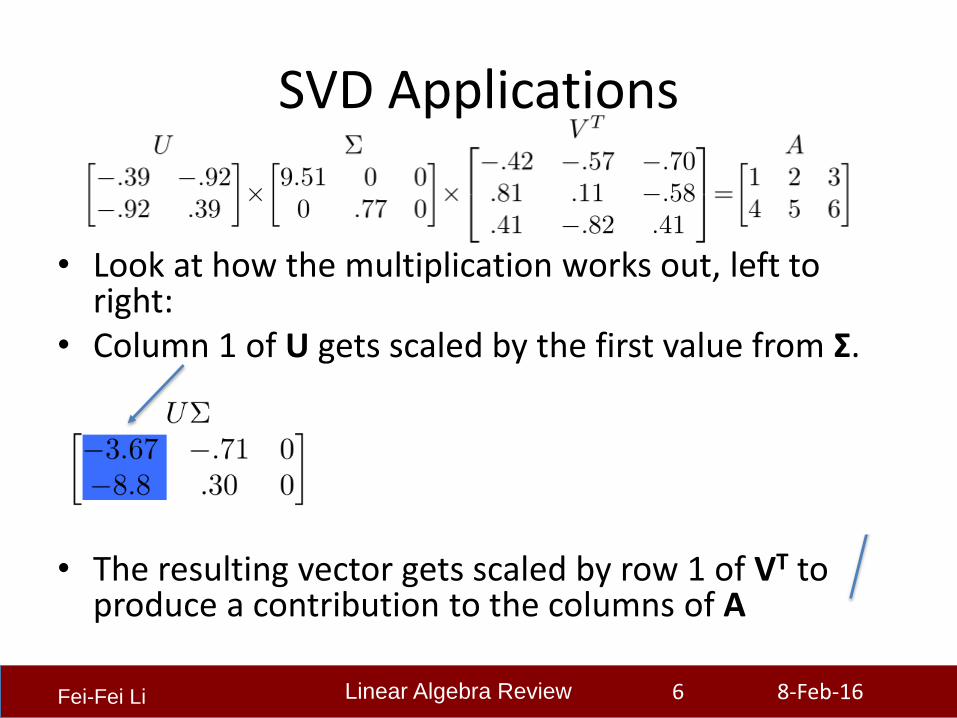
• Look at how the multiplication works out, left to right:

• Column 1 of U gets scaled by the first value from Σ.

• The resulting vector gets scaled by row 1 of VT to produce a contribution to the columns of A

SVD Applications

8-Feb-166


SVD Applications

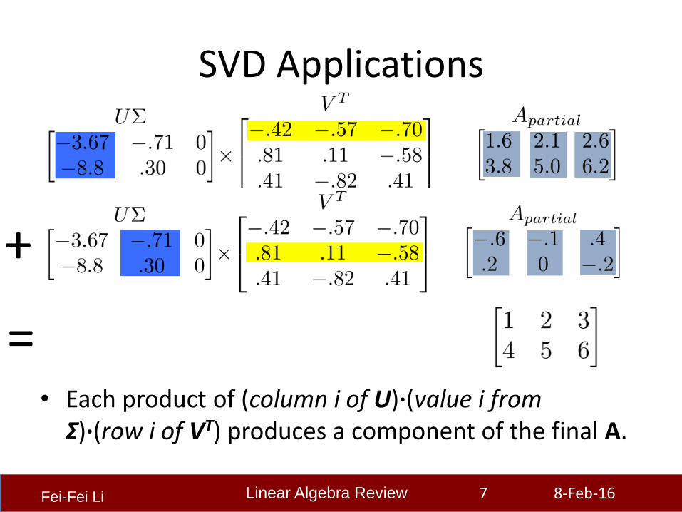
• Each product of (column i of U)∙(value i from Σ)∙(row i of VT) produces a component of the final A.

8-Feb-167

+

=


SVD Applications

• We’re building A as a linear combination of the columns of U

• Using all columns of U, we’ll rebuild the original matrix perfectly

• But, in real-world data, often we can just use the first few columns of U and we’ll get something close (e.g. the first Apartial, above)

8-Feb-168


SVD Applications

• We can call those first few columns of U the Principal Components of the data

• They show the major patterns that can be added to produce the columns of the original matrix

• The rows of VT show how the principal componentsare mixed to produce the columns of the matrix

8-Feb-169


SVD Applications

We can look at Σ to see that the first column has a large effect

8-Feb-1610

while the second column has a much smaller effect in this example


Principal Component Analysis

• Often, raw data samples have a lot of redundancy and patterns

• PCA can allow you to represent data samples as weights on the principal components, rather than using the original raw form of the data

• By representing each sample as just those weights, you can represent just the “meat” of what’s different between samples

• This minimal representation makes machine learning and other algorithms much more efficient

8-Feb-1611


Addendum: How is SVD computed?

• For this class: tell MATLAB to do it: [U,S,V] = svd(A);

• But, if you’re interested, one computer algorithm to do it makes use of Eigenvectors

– The following material is presented to make SVD less of a “magical black box.” But you will do fine in this class if you treat SVD as a magical black box, as long as you remember its properties from the previous slides.

8-Feb-1612


Eigenvector definition

• Suppose we have a square matrix A. We can solve for vector x and scalar λ such that Ax= λx

• In other words, find vectors where, if we transform them with A, the only effect is to scale them with no change in direction.

• These vectors are called eigenvectors (German for “self vector” of the matrix), and the scaling factors λ are called eigenvalues

• An m x m matrix will have ≤ m eigenvectors where λ is nonzero

8-Feb-1613


Finding eigenvectors

• Computers can find an x such that Ax= λx using this iterative algorithm:

– x=random unit vector– while(x hasn’t converged)

• x=Ax• normalize x

• x will quickly converge to an eigenvector• Some simple modifications will let this algorithm

find all eigenvectors

8-Feb-1614


Finding SVD

• Eigenvectors are for square matrices, but SVD is for all matrices

• To do svd(A), computers can do this:

– Take eigenvectors of AAT (matrix is always square).

• These eigenvectors are the columns of U.

• Square root of eigenvalues are the singular values (the entries of Σ).

– Take eigenvectors of ATA (matrix is always square).

• These eigenvectors are columns of V (or rows of VT)

8-Feb-1615


Finding SVD

• Moral of the story: SVD is fast, even for large matrices

• It’s useful for a lot of stuff• There are also other algorithms to compute SVD

or part of the SVD– MATLAB’s svd() command has options to efficiently

compute only what you need, if performance becomes an issue

8-Feb-1616

A detailed geometric explanation of SVD is here:http://www.ams.org/samplings/feature-column/fcarc-svd

http://www.ams.org/samplings/feature-column/fcarc-svd

Slide credit: Alexander Ihler

( ) ( )

Slide credit: Alexander Ihler

Dimensionality Reduction

Slide credit: Erik Sudderth

Principal Components Analysis

Slide credit: Subhransu Maji

Lagrange Multipliers

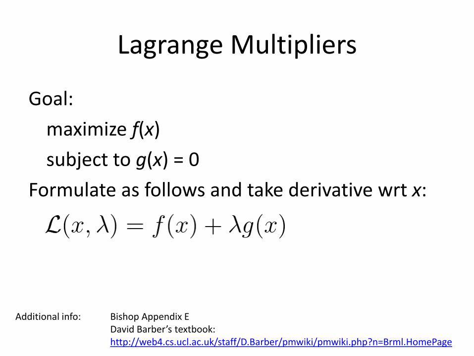
Goal:

maximize f(x)

subject to g(x) = 0

Formulate as follows and take derivative wrt x:

Additional info: Bishop Appendix EDavid Barber’s textbook: http://web4.cs.ucl.ac.uk/staff/D.Barber/pmwiki/pmwiki.php?n=Brml.HomePage

http://web4.cs.ucl.ac.uk/staff/D.Barber/pmwiki/pmwiki.php?n=Brml.HomePage

Principal Components Analysis

Slide credit: Subhransu Maji

Limitations

• PCA preserves maximum variance

• A more discriminative subspace:

Fisher Linear Discriminants

• FLD preserves discrimination

– Find projection that maximizes scatter between classes and minimizes scatter within classes

Reference: Eigenfaces vs. Fisherfaces, Belheumer et al., PAMI 1997

Adapted from Derek Hoiem

WARNING: SUPERVISED

http://citeseerx.ist.psu.edu/viewdoc/download?doi=10.1.1.10.3247&rep=rep1&type=pdf

Illustration of the Projection

Poor Projection

x1

x2

x1

x2

Using two classes as example:

Good

Slide credit: Derek Hoiem

WARNING: SUPERVISED

Plan for today

• Review

– PCA wrap-up


– Regularization


Why do we cluster?

• Summarizing data– Look at large amounts of data

– Represent a large continuous vector with the cluster number

• Counting– Computing feature histograms

• Prediction– Data in the same cluster may have the same labels

Slide credit: J. Hays, D. Hoiem

0 190 255

• Goal: choose three “centers” as the data

representatives, and label every data point according

to which of these centers it is nearest to.

• Best cluster centers are those that minimize SSD

between all points and their nearest cluster center ci:

1-D data

Source: K. Grauman

Clustering

• With this objective, it is a “chicken and egg” problem:

– If we knew the cluster centers, we could allocate

points to groups by assigning each to its closest center.

– If we knew the group memberships, we could get the

centers by computing the mean per group.

Source: K. Grauman

Clustering

K-means clustering

• Basic idea: randomly initialize the k cluster centers, and

iterate between the two steps we just saw.

1. Randomly initialize the cluster centers, c1, ..., cK

2. Given cluster centers, determine points in each cluster

• For each point p, find the closest ci. Put p into cluster i

3. Given points in each cluster, solve for ci

• Set ci to be the mean of points in cluster i

4. If ci have changed, repeat Step 2

Properties• Will always converge to some solution

• Can be a “local minimum”

• does not always find the global minimum of objective function:

Source: Steve Seitz

Source: A. Moore

Application: Segmentation as clustering

Depending on what we choose as the feature space, we

can group pixels in different ways.

Grouping pixels based

on intensity similarity

Feature space: intensity value (1-d)

Source: K. Grauman

K=2

K=3

quantization of the feature space;

segmentation label map

Source: K. Grauman

K-means: pros and cons

Pros• Simple, fast to compute

• Converges to local minimum of within-cluster squared error

Cons/issues• Setting k?

– One way: silhouette coefficient

• Sensitive to initial centers– Use heuristics or output of another method

• Sensitive to outliers

• Detects spherical clusters

Adapted from K. Grauman

• The mean shift algorithm seeks modes or local

maxima of density in the feature space

Mean shift algorithm

imageFeature space

(L*u*v* color values)

Source: K. Grauman

Search

window

Center of

mass

Mean Shift

vector

Mean shift

Slide by Y. Ukrainitz & B. Sarel

Search

window

Center of

mass

Mean shift


Points in same cluster converge

Source: D. Hoiem

• Cluster: all data points in the attraction basin

of a mode

• Attraction basin: the region for which all

trajectories lead to the same mode

Mean shift clustering


Simple Mean Shift procedure:

• Compute mean shift vector

•Translate the Kernel window by m(x)

2

1

2

1

( )

ni

i

i

ni

i

gh

gh

x - xx

m x xx - x

Computing the Mean Shift


Kernel density estimation

Kernel

Data (1-D)

Estimated

density

Source: D. Hoiem

• Compute features for each point

• Initialize windows at individual feature points

• Perform mean shift for each window until convergence

• Merge windows that end up near the same “peak” or mode

Mean shift clustering

Source: D. Hoiem

• Pros:– Does not assume shape on clusters

– Robust to outliers

• Cons/issues:– Need to choose window size

– Does not scale well with dimension of feature space

– Expensive: O(I n2)

Mean shift

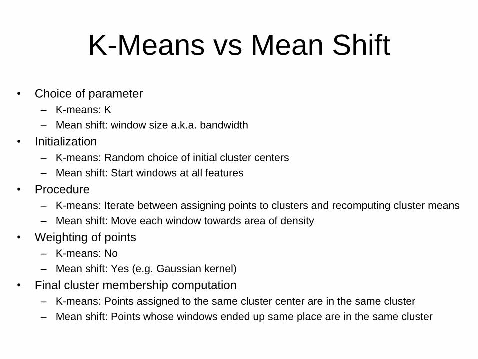
K-Means vs Mean Shift

• Choice of parameter

– K-means: K

– Mean shift: window size a.k.a. bandwidth

• Initialization

– K-means: Random choice of initial cluster centers

– Mean shift: Start windows at all features

• Procedure

– K-means: Iterate between assigning points to clusters and recomputing cluster means

– Mean shift: Move each window towards area of density

• Weighting of points

– K-means: No

– Mean shift: Yes (e.g. Gaussian kernel)

• Final cluster membership computation

– K-means: Points assigned to the same cluster center are in the same cluster

– Mean shift: Points whose windows ended up same place are in the same cluster

Plan for today

• Review

– PCA wrap-up


– Regularization


Bias-Variance Trade-off

• Models with too few parameters are inaccurate because of a large bias (not enough flexibility).

• Models with too many parameters are inaccurate because of a large variance (too much sensitivity to the sample).

Adapted from D. Hoiem

Red dots = training data (all that we see before we ship off our model!)

Green curve = true underlying model Blue curve = our predicted model/fit

Purple dots = possible test points

Think about “squinting”…

Over-fitting

Slide credit: Chris Bishop

Regularization

Penalize large coefficient values

(Remember: We want to minimize this expression.)

Adapted from Chris Bishop

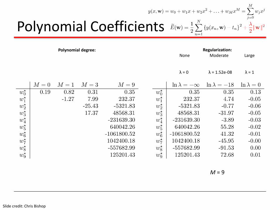
Polynomial Coefficients


Regularization:None Moderate Large

λ = 0 λ = 1.52e-08 λ = 1

Polynomial degree:

M = 9

Regularization:


λ = 1.52e-08

Regularization:


λ = 1

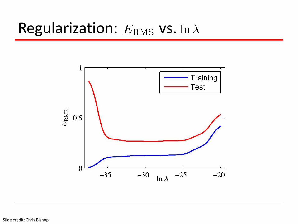
Regularization: vs.


Normalization vs Regularization

Normalization/standardization:

• Scaling the features (the xi’s)

• E.g. if each xi is a word count and there are many words in that particular document, normalize each word count to control magnitude of entire x vector

Regularization:

• Scaling the feature weights (the wi’s) a.k.a. the model parameters

• Preventing the model from caring too much about any single word

How to reduce over-fitting?

• Get more training data

• Regularize the parameters

• Use fewer features

• Choose a simpler classifier

Slide credit: D. Hoiem

Bias-variance tradeoff

Training error

Test error

Underfitting Overfitting

Complexity Low Bias

High Variance

High Bias

Low Variance

Err

or


Bias-variance tradeoff

Many training examples

Few training examples

Complexity Low Bias

High Variance

High Bias

Low Variance

Test E

rror


Effect of Training Size

Testing

Training

Generalization Error

Number of Training Examples

Err

or

Fixed prediction model


Summary

• Three kinds of error

– Inherent: unavoidable

– Bias: due to over-simplifications

– Variance: due to inability to perfectly estimate parameters from limited data

• Use increasingly powerful classifiers with more training data (bias-variance trade-off)


Plan for today

• Review

– PCA wrap-up


– Regularization


cs 2750: machine learning review (cont’d)

Documents