Crude Oil Prices: Trends and Forecast

Noureddine Krichene

WP/08/133

© 2008 International Monetary Fund WP/08/133 IMF Working Paper African Department

Crude Oil Prices: Trends and Forecast

Prepared by Noureddine Krichene1

Authorized for distribution by Benedicte Vibe Christensen

May 2008

Abstract

This Working Paper should not be reported as representing the views of the IMF. The views expressed in this Working Paper are those of the author(s) and do not necessarily represent those of the IMF or IMF policy. Working Papers describe research in progress by the author(s) and are published to elicit comments and to further debate.

Following record low interest rates and fast depreciating U.S. dollar, crude oil prices became under rising pressure and seemed boundless. Oil price process parameters changed drastically in 2003M5–2007M10 toward consistently rising prices. Short-term forecasting would imply persistence of observed trends, as market fundamentals and underlying monetary policies were supportive of these trends. Market expectations derived from option prices anticipated further surge in oil prices and allowed significant probability for right tail events. Given explosive trends in other commodities prices, depreciating currencies, and weakening financial conditions, recent trends in oil prices might not persist further without triggering world economic recession, regressive oil supply, as oil producers became wary about inflation. Restoring stable oil markets, through restraining monetary policy, is essential for durable growth and price stability. JEL Classification Numbers: C22, E31, E52, Q41, Q43. Keywords: Characteristic function, crude oil prices, density forecast, Esscher transform, Fourier

transform, inverse problem, normal inverse Gaussian, monetary policy, option prices. Author’s E-Mail Address: nkrichene@imf.org - nnkrichene@hotmail.com

1 The author expresses deep gratitude to Abbas Mirakhor, Benedicte Christensen, John Wakeman-Linn, Geneviève Labeyrie, Helen Lynch, Valerie Mercer-Blackman, Kevin Cheng, and Ibrahim Gharbi from Islamic Development Bank.

2

Contents

Page

I. Introduction.......................................................................................................................3

II. Recent Evolution of Oil Prices .........................................................................................4

III. Modeling Oil Prices as Levy Process ...............................................................................7

IV. Oil Price Process as Normal Inverse Gaussian Process....................................................8

V. Estimation of Oil Price Process as a Normal Inverse Gaussian Process ........................10

VI. Market Incompleteness and Esscher Transform.............................................................12

VII. Density Forecast of Crude Oil Prices: The Inverse Problem..........................................14

VIII. Conclusions.....................................................................................................................18

Tables 1. Descriptive Statistics for Oil Price Returns ...........................................................................6 2. Oil Price as Normal Inverse Distribution, Parameterization ...............................................10 3. Oil Price as Normal Inverse Distribution, Parameterization ...............................................10 Figures 1. Oil Daily Futures Prices, January 2000–October 2007 .........................................................4 2a. Empirical Distribution of Oil Price Returns 2000M1–2003M4 ..........................................6 2b. Empirical Distribution of Oil Price Returns, 2003M5–2007M10 .......................................6 3. Oil Price Returns GARCH(1.1) Volatility, January 2000-October 2007 ..............................6 References................................................................................................................................21

3

I. INTRODUCTION

By maintaining upward persistence since early 2003 and breaking new record of US$120/barrel in April 2008, crude oil prices remained under intense pressure and seemed boundless; their rapid pace may turn inflationary by causing other prices to rise and may decelerate world economic growth. All the more worrisome, recent upsurges in oil prices were taking place in midst of rising trends in commodity prices, instability in housing, equity, and credit markets, and depreciating exchange rates. The fast rise in commodities prices, including oil, could be seen as delayed effect of excessively expansionary monetary policies during 2001–04 when key interest rates were forced down to postwar record levels. Such monetary expansion led to high world economic growth and consequently higher world demand for oil and non-oil commodities. Supply of crude oil and other commodities being rigid or lagging at smaller pace, excess demand resulted in highest inflation for postwar commodities markets. With real interest rates turning low or negative, pressure on real aggregate demand, and therefore on oil markets, might not subside. Relaxation of monetary policy in August 2007─March 2008 immediately set off new spiral in commodities price inflation and currency depreciation.2 This paper analyzed oil prices during 2000M1–2007M10. To exhibit effect of monetary policy, the paper distinguished two samples 2000M1–2003M4 and 2003M5–2007M10. The paper assumed oil prices to be driven by Levy processes (LP) of generalized hyperbolic (GH) type and used daily data to estimate parameters of these processes. Combining features of normal and stable distributions and offering more flexibility than Poisson-type processes, which were known to model finite large jumps, GH distributions gained wide popularity in modeling stock market indices. In view of their success in modeling financial time-series, Levy processes of hyperbolic type were advocated by many authors. In this respect, the hyperbolic distribution was proposed for modeling LP by Barndorff-Nielsen (1977), Barndorff-Nielsen and Blaesild (1983), Bibby and Sørensen (1997 and 2003), Eberlein and Keller (1995), and Prause (1999). The normal inverse Gaussian (NIG) distribution was proposed by Barndorff-Nielsen (1995), and Rydberg (1997); and the variance gamma distribution was applied by Madan et al. (1998). GH processes became appealing for their ability to account for salient features of high frequency financial time-series, namely asymmetry, frequent small and large jumps, and to reduce the smile in option prices (Eberlein et al. 1998). Inability of Gaussian processes to fit high frequency financial data was underscored by Fama (1965) and Mandelbrot (1963); both authors proposed stable distributions for modeling skewness and kurtosis; however, stable distributions did not have finite variance and therefore were not appealing for modeling financial time-series. Besides ability to account for skewness and kurtosis, GH distributions enabled to remedy shortcomings noted in Black-Scholes model (1973) with respect to implausibility of the normality assumption and constancy of the variance of the distribution. To the extent that GH distributions were constructed as mixtures of variance-mean normal distribution with time varying stochastic variance, or equivalently, as Brownian

2 In August 2007─March 2008, some key discount rates were cut, large amounts of liquidities were injected, and successive cuts in the federal funds rate were undertaken. Multi-billion bail out facilities were put in place to rescue banks with nonperforming portfolios

4

motion subordinated to increasing positive stochastic processes, they can account for stochastic volatility and allow to attenuate the smile in short-term options (Carr et al. 2003). As a precursor to application of subordinated process for fitting financial time-series was Clark’s paper (1973) which introduced Bochner’s concept of a subordinate stochastic process as a model for speculative price series. Clark showed that the concept of subordination allows to use finite variance distribution, and obtain a mixture distribution, where the mixing distribution is an increasing positive Levy process that has finite moments. He showed, with both discrete Bayes' test and Kolmogorov-Smirnov test, that finite-variance distributions subordinate to the normal, namely a lognormal-normal distribution, fit cotton futures price data better than members of the stable family. This paper showed that Normal Inverse Gaussian (NIG) process fits closely oil price returns during 2000M1–2003M4 and 2003M5–2007M10; parameters of the process had, however, changed; mean return increased due to persistence in upward trend, and kurtosis had declined due to higher predictability in oil prices. Estimated parameters of the NIG process were in conformity with findings for the empirical distribution of oil price returns. To be applicable for pricing derivatives, statistical distributions had to be adjusted for market price of risk and turned into martingale processes. This is done through applying Esscher transform to the statistical process. Besides estimating oil price returns distribution from time-series data, oil price returns distribution was also estimated from cross-section data from call and put option prices on November 2, 2007 for end-December 2007. Implied-risk neutral distribution based on NIG showed that traders were expecting further rise in oil prices and were assigning significant probabilities for right-tail events. The paper was structured as follows: Section II studied daily oil prices during 2000M1–2007M10; Section III presented the theoretical framework for Levy processes; Section IV presented the normal inverse Gaussian (NIG) distribution; Section V presented the statistical estimation of the NIG distribution based on daily oil price data for 2000M1–2003M4 and 2003M5–2007M10; Section VI derived risk-neutral distributions from statistical LP by applying Esscher transform to these processes; Section VII derived density forecast from oil options prices; Section VIII concluded.

II. RECENT EVOLUTION OF OIL PRICES

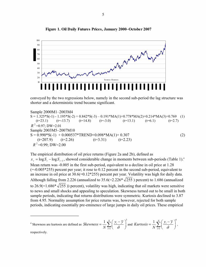
Daily data of light crude futures prices from January 4, 2000 to October 29, 2007 was considered (Figure 1) 3. The behavior of oil prices showed distinctly two patterns: relative stability during 2000M1–2003M4, around a mean of US$27 per barrel, and strong upward deterministic trend and persistence during 2003M5–2007M10, with prices rising progressively to cross US$96/barrel mark in October 2007, showing no sign for stability around a mean. The upward trend became predictable and was the longest upward trend in post-war oil prices. Past upward trends lived on average two to three years, while the present one has spanned so far more than four years. Denoting oil price by tS and applying an autoregressive moving average (ARMA) representation, the structure of the oil price process has changed considerably as 3 Light crude futures prices from Reuters, 1986 observations.

5

Figure 1. Oil Daily Futures Prices, January 2000–October 2007

10

20

30

40

50

60

70

80

90

100

So urce: Reuters

conveyed by the two regressions below, namely in the second sub-period the lag structure was shorter and a deterministic trend became significant. Sample 2000M1–2003M4 S = 1.325*S(-1) - 1.195*S(-2) + 0.842*S(-3) – 0.191*MA(1)+0.778*MA(2)+0.214*MA(3)+0.769 (1) (t=23.1) (t=-13.7) (t=14.8) (t=-3.0) (t=13.1) (t=6.1) (t=2.7)

2R =0.97; DW=2.01 Sample 2003M5–2007M10 S = 0.990*S(-1) + 0.000537*TREND+0.098*MA(1)+ 0.307 (2) (t=207.9) (t=2.26) (t=3.31) (t=2.23) 2R =0.99; DW=2.00 The empirical distribution of oil price returns (Figure 2a and 2b), defined as

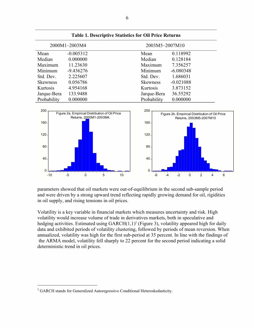
1log logt t tx S S −= − , showed considerable change in moments between sub-periods (Table 1).4 Mean return was -0.005 in the first sub-period, equivalent to a decline in oil price at 1.28 (=-0.005*255) percent per year; it rose to 0.12 percent in the second sub-period, equivalent to an increase in oil price at 30.6(=0.12*255) percent per year. Volatility was high for daily data. Although falling from 2.226 (annualized to 35.6(=2.226* 255 ) percent) to 1.686 (annualized to 26.9(=1.686* 255 )) percent), volatility was high, indicating that oil markets were sensitive to news and small shocks and appealing to speculation. Skewness turned out to be small in both sample periods, indicating that returns distributions were symmetric. Kurtosis declined to 3.87 from 4.95. Normality assumption for price returns was, however, rejected for both sample periods, indicating essentially pre-eminence of large jumps in daily oil prices. These empirical

4 Skewness are kurtosis are defined as 3

1

1ˆ

Ni

i

y ySkewnessN σ=

−⎛ ⎞= ⎜ ⎟⎝ ⎠

∑ and 4

1

1ˆ

Ni

i

y yKurtosisN σ=

−⎛ ⎞= ⎜ ⎟⎝ ⎠

∑ ,

respectively.

6

Table 1. Descriptive Statistics for Oil Price Returns

2000M1–2003M4 2003M5–2007M10 Mean -0.005312 Median 0.000000 Maximum 11.23630 Minimum -9.436276 Std. Dev. 2.225607 Skewness 0.056786 Kurtosis 4.954168 Jarque-Bera 133.9488 Probability 0.000000

Mean 0.118992 Median 0.128184 Maximum 7.356257 Minimum -6.080348 Std. Dev. 1.686031 Skewness -0.021088 Kurtosis 3.873152 Jarque-Bera 36.55292 Probability 0.000000

0

40

80

120

160

200

-10 -5 0 5 10

Figure 2a. Empirical Distribution of Oil Price Returns, 2000M1-2003M4.

0

40

80

120

160

200

-6 -4 -2 0 2 4 6

Figure 2b. Empirical Distribution of Oil Price Returns, 2003M5-2007M10

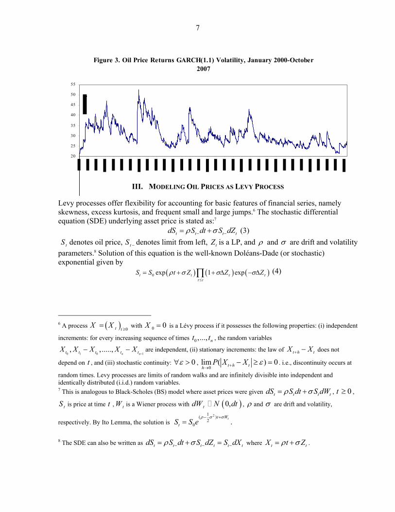
parameters showed that oil markets were out-of-equilibrium in the second sub-sample period and were driven by a strong upward trend reflecting rapidly growing demand for oil, rigidities in oil supply, and rising tensions in oil prices. Volatility is a key variable in financial markets which measures uncertainty and risk. High volatility would increase volume of trade in derivatives markets, both in speculative and hedging activities. Estimated using GARCH(1,1)5 (Figure 3), volatility appeared high for daily data and exhibited periods of volatility clustering, followed by periods of mean reversion. When annualized, volatility was high for the first sub-period at 35 percent. In line with the findings of the ARMA model, volatility fell sharply to 22 percent for the second period indicating a solid deterministic trend in oil prices.

5 GARCH stands for Generalized Autoregressive Conditional Heteroskedasticity.

7

Figure 3. Oil Price Returns GARCH(1.1) Volatility, January 2000-October 2007

20

25

30

35

40

45

50

55

III. MODELING OIL PRICES AS LEVY PROCESS

Levy processes offer flexibility for accounting for basic features of financial series, namely skewness, excess kurtosis, and frequent small and large jumps.6 The stochastic differential equation (SDE) underlying asset price is stated as:7

t t t tdS S dt S dZρ σ− −= + (3) tS denotes oil price, tS − denotes limit from left, tZ is a LP, and ρ and σ are drift and volatility parameters.8 Solution of this equation is the well-known Doléans-Dade (or stochastic) exponential given by

( ) ( ) ( )0 exp 1 expt tt

S S t Z Z Zτ ττ

ρ σ σ σ≤

= + + Δ − Δ∏ (4)

6 A process ( ) 0t t

X X≥

= with 0 0X = is a Lévy process if it possesses the following properties: (i) independent

increments: for every increasing sequence of times 0 ,..., nt t , the random variables

0 1 0 1, ,.....,

n nt t t t tX X X X X−

− − are independent, (ii) stationary increments: the law of t h tX X+ − does not

depend on t , and (iii) stochastic continuity: 0ε∀ > , 0

lim ( ) 0t h thP X X ε+→

− ≥ = . i.e., discontinuity occurs at

random times. Levy processes are limits of random walks and are infinitely divisible into independent and identically distributed (i.i.d.) random variables. 7 This is analogous to Black-Scholes (BS) model where asset prices were given t t t tdS S dt S dWρ σ= + , 0t ≥ ,

tS is price at time t , tW is a Wiener process with ( )0,tdW N dt , ρ and σ are drift and volatility,

respectively. By Ito Lemma, the solution is 21( )

20

tt W

tS S eρ σ σ− +

= . 8 The SDE can also be written as t t t t t tdS S dt S dZ S dXρ σ− − −= + = where t tX t Zρ σ= + .

8

Here Z Z Zτ τ τ −Δ = − denotes jump at time τ . Clearly, the condition ( )1 0Zτσ+ Δ ≥ has to hold

for tS to be nonnegative, i.e., 0tS ≥ . Thus, jumps are bounded below by 1Zτ σΔ ≥ − . Obviously,

solution (4) does not enable easy manipulation of the price process such as computation of compounded returns or simulation of the price path. To obtain an easier form for LP, the SDE is reformulated as 9

( ) ( )1 1t tZ Zt t t t t t t t t tdS S dt S dZ S e Z S dt S dZ e Zσ σρ σ σ ρ σ σΔ Δ

− − − − −= + + − − Δ = + + − − Δ (5) Similar to a Poisson process, jumps now appear explicitly in the dynamics of the oil process. This representation of SDE arises from an application of Ito’s formula, and yields a simpler solution for the price process:

( )0 expt tS S t Zρ σ= + (6)

IV. OIL PRICE PROCESS AS NORMAL INVERSE GAUSSIAN PROCESS

In this section, oil price returns, defined as 1 1log logt t t t tx S S X X− −= − = − , are analyzed as a normal inverse Gaussian (NIG) distribution, where ( )0 expt tS S X= . NIG distribution is a

special case of the generalized hyperbolic distribution ( )GH . The GH distribution was essentially due to Barndorff-Nielsen (1977). Let X be a normal distribution, i.e.

( ),X N z zμ β+ and let Z be a generalized inverse Gaussian (GIG) law, i.e.

( ), ,Z GIG λ δ γ . Define X Z V Zμ β= + + , where ( )0,1V N , then X is said to have a GH distribution obtained as a normal variance-mean mixture where the mixing distribution is

( ), ,Z GIG λ δ γ ; or equivalently, X is obtained as a normal distribution subordinated to a GIG process. It is written as:

0

( ; , , , , ) ( ; , ) ( ; , , )GH Normal GIGf x f x z z f z dzλ α β δ μ μ β λ δ γ∞

= +∫ (7)

Let 2 2γ α β= − , the parameters of the GH distribution areμ , δ , α , β , andλ . They measure location ( )μ , scale ( )δ , steepness of tail ( )α , skewness of distribution ( )β , and

distribution class ( )λ . Parameters must satisfy: Rλ∈ , Rμ ∈ , 0δ ≥ , and 0 β α≤ < . GH distribution has more parameters than either stable or normal distribution and provides therefore more flexibility for controlling skewness and tail thickness of the distribution. Parameters α and β are also called shape parameters; higher value for α indicates steeper tail, and β =0 indicates symmetric distribution. Different parameterizations for distribution shape are proposed (see Prause, 1999), which are:

9 If the SDE is formulated as t t tdS S dX−= , the reformulated SDE will be

( )1tXt t tt

d S S d X e X−

Δ= + − −Δ .

9

First parameterization:, α , β ,δ ,μ ; 2nd parameterization 2 2ζ δ α β= − ,βρα

= ,δ ,μ ;

3rd parameterization ( )121ξ ζ −= + , χ ξρ= ,δ ,μ ; and 4th parameterization α αδ= , β βδ= ,δ ,μ .

NIG distribution was introduced by Barndorff–Nielsen (1995) as a subclass of GH laws

obtained for21

−=λ .10 The density function for NIG is:

( ) ( )( )( )( )

( )

221

2 2

22; , , , exp

K xnig x x

x

α δ μδαα β δ μ δ α β β μπ δ μ

+ −= − + −

+ −

(8)

where , ,0 ,0x Rμ δ β α∈ ≤ ≤ ≤ ,and K1 is modified Bessel function of third kind with index 1.11 Let 2 2γ α β= − , moments of NIG are:

[ ]E X βμ δγ

⎛ ⎞= + ⎜ ⎟

⎝ ⎠ (9)

[ ]2

3Var X αδγ

⎛ ⎞= ⎜ ⎟

⎝ ⎠ (10)

[ ] 1 2

13( )

Skew X βα δ γ

⎛ ⎞⎛ ⎞= ⎜ ⎟⎜ ⎟⎝ ⎠ ⎝ ⎠

(11)

[ ]2 13 1 4

( )Kurt X β

α δ γ⎛ ⎞ ⎛ ⎞⎛ ⎞= +⎜ ⎟ ⎜ ⎟⎜ ⎟⎜ ⎟⎝ ⎠ ⎝ ⎠⎝ ⎠

(12)

The moment generating function (MGF) of NIG is:

( )2 22 2 2 2

2 2

( )

( )( )

u uuNIG u

eM u e ee

δ α β μ δ α β α βμ

δ α β

− + − − − +

− += = (13)

satisfying uβ α+ < . Simulation of NIG for forecast purpose was studied by Rydberg (1997) based on algorithms developed by Dagpunar (1989).

10 Thus, ( , , , , 1/ 2) ( , , , )GH NIGα β μ δ λ α β μ δ= − = . NIG process can be related to a Brownian motion time-

changed by an Inverse Gaussian process (IG). Let { , 0}tW W t= ≥ be a Brownian motion and let

{ , 0}tIG IG t= ≥ be an IG process with parameters 1a = and 2 2b δ α β= − , with 0α > ,

α β α− < < and 0δ > ; then the process: ( )2.t t tX IG W IGβδ δ= + is an ( , , )NIG α β δ process with

parameters , ,α β δ . An equivalent parameterization of NIG process is a Brownian motion with drift θ and

volatilityσ , ( ) ( )B t t W tθ σ= + , computed at random time given by a gamma process (1, )G υ :

( ; , , ) . ( )NIG t tX t G W Gυ υσ υ θ θ σ= + .

11 Specifically, 2

21

0

( ) exp4 4x xK x t t dt

t

∞−⎡ ⎤

= +⎢ ⎥⎣ ⎦

∫ , x R∈ .

10

NIG motion, as well as other subclasses of hyperbolic distributions, is LP that has the property of being pure jump and infinite activity models. Its representation as time-changed Brownian motion allows modeling time change which itself reflects the intensity of economic activity through news arrival and trades. Tractability of the characteristic function (CF) of the NIG and other subclasses of the GH allows to recover option prices through fast Fourier transform (FFT). Knowledge of CF enables to recover the probability distribution through numerical inversion (Davies, 1973) as:

0

1 1 ( ) ( )( )2 2

iux iuxe u e uF x duiu

φ φπ

∞ −− −= + ∫ (14)

Empirical performance of GH distributions in modeling skewness, kurtosis, and implied volatility smile in option prices made them more appealing than classical diffusion or jump-diffusion models. The hyperbolic law was found to provide a very good model for distributions of daily stock returns for a number of leading German enterprises (Eberlein and Keller, 1995), giving way to its today's use in stock price modeling (Bibby and Sørensen, 1997) and market risk measurement (Eberlein et al., 1998). Eberlein et al. (1998) showed that the hyperbolic distribution allows an almost perfect fit to financial data, both in spot and derivatives markets.

V. ESTIMATION OF OIL PRICE PROCESS AS A NORMAL INVERSE GAUSSIAN PROCESS

Estimation of the NIG distribution used the R program and the statistical packages: HyperbolicDist, ghyp, and fBasics package.12, 13

Table 2: Oil Price as Normal Inverse Distribution, Parameterization ( ), , ,α β δ μ

Parameters Moments Alpha Beta Delta Mu Mean Variance Skewness Kurtosis

2000M1–2003M4 0.54 -0.02 2.69 0.08 -0.005 4.92 -0.08 1.72 2003M5–2007M10 0.97 -0.06 2.76 0.29 0.12 2.86 -0.11 1.13

Table 3: Oil Price as Normal Inverse Distribution, Parameterization ( ), , , ,λ α μ σ β

Parameters Moments

Lambda

Alpha.bar Shape parameter

Mu Location parameter

Sigma Dispersion parameter

Beta Skewness parameter

Mean Variance Skewness Kurtosis

2000M1–2003M4 -0.5 1.46 0.08 2.22 -0.08

-0.005 4.95 -0.08 2.06

2003M5–2007M10 -0.5 2.68 0.29 1.69 -0.17 0.12 2.87 -0.04 1.22 12 http://www.r-project.org/;The HyperbolicDist Package, David Scott d.scott@auckland.ac.nz; The Ghyp Package, Wolfgang Breymann, David Luethi, david.luethi@zhwin.ch; The fBasics Package, Diethelm Wuertz, wuertz@itp.phys.ethz.ch.

13Because characteristic function of NIG is known in closed form, parameter estimation can also be performed using the empirical characteristic function method (See Parzen 1962, Feuerverger and McDunnough, 1981).

11

Estimation of the oil price NIG distribution yielded results consistent with findings for empirical distributions in Section II; namely, NIG parameters changed significantly in 2003M5–2007M10 compared with 2000M1–2003M4 under strong impulses from monetary policy. Location parameter μ increased from 0.08 to 0.29. Consequently, mean return increased from -0.005 (annualized to-0.005*255= -1.28 percent) in 2000M1–2003M4 to 0.12 (annualized to 30.6 percent) in 2003M5–2007M10. Scale parameterδ increased slightly from 2.69 to 2.76; however, by exceeding unity, it remained high, indicating a stretched out distribution. Shape parameter measuring skewness β remained small in the range -0.02–-0.06 indicating symmetric oil price returns distribution. Shape parameter measuring tail steepness α increased significantly from 0.54 in 2000M1–2003M4 to 0.97 in 2003M5–2007M10, indicating steeper tails and therefore higher frequency of smaller jumps. Consequently, volatility fell considerably, from 2.2 in 2000M1–2003M4 (annualized to 35 percent) to 1.7 in 2003M5–2007M10 (annualized to 27 percent). In spite this decline, volatility remained high for daily data, implying that oil markets were constantly facing significant uncertainty and were sensitive to news and small shocks and attractive to speculators. In sum, parameter estimates for two sub-samples were fully concordant with data. They established that oil price process was dominated by a jump process, with distinct features. In 2000M1–2003M4, oil prices exhibited high volatility, however, distribution mean was small and negative, indicating that the oil process fluctuated widely around a slightly declining trend. In 2003M5–2007M10, oil price process showed declining volatility; however, it was driven by a sharply upward trend, annualized to 30.6 percent per year, meaning that oil markets were permanently out-of-equilibrium during this period. While density was symmetric in both sub-periods, meaning that probability of upward jumps was matched by probability of downward jumps, the drift component of the process became powerful in the second sub-period and drove oil prices on a rising trend. These parameters estimates can be explained by world demand and supply for crude oil and underlying fundamentals for crude oil markets.14 As world real GDP expanded at 4–5.5 percent per year during 2003–07 and U.S. dollar kept depreciating, world oil demand for oil expanded faster than before. Given rigidities in world oil supply, faster growth of oil demand created excess demand for oil. Given short-term inelasticity of oil demand and supply with respect to prices, any small excess demand for oil would cause large variation in prices. In turn, large price increases would have small negative effect on oil demand. Negative price effect, however, would be quickly dominated by positive income effect, i.e., world economic growth, which kept oil prices under rising pressure.

14 Simultaneous demand-supply models for world oil markets were analyzed in Krichene (2002, 2005, 2006, and 2007). In these models, world real GDP, interest and exchange rates were shown to be key driving variables of oil demand, and consequently, main determinants of oil prices.

12

VI. MARKET INCOMPLETENESS AND ESSCHER TRANSFORM

This section studies risk-neutral distribution, or equivalently, martingale measure,15 associated with statistical NIG. Such martingale measure is used for pricing derivatives based on NIG process. Indeed, except for Brownian motion or Poisson process, LP are incomplete models. A perfect hedge cannot be obtained and there is always a residual risk which cannot be hedged. In a Levy market, there are many different equivalent martingale measures under which discounted asset price process is a martingale. Existence of martingale measure is related to absence of arbitrage, while uniqueness of martingale measure is related to market completeness, i.e., perfect hedging. One approach for finding an equivalent martingale measure is Esscher transform proposed by Gerber and Shiu (1994). Given a statistical distribution P , Esscher transform induces an equivalent probability measureQ and a martingale process. Esscher parameter is determined so that discounted asset price is a martingale under the new probability measure Q . Let

( )( ) (0) X tS t S e= , where 0{ ( )}tX t ≥ is an LP with stationary and independent increments and (0) 0X = . For each t , the random variable ( )X t , seen as the continuous compounded rate of

return over t periods, has an infinitely divisible distribution with a probability density given

by ( , )f x t , 0t > . MGF, assumed to exist, is defined as ( )( , ) [ ] ( , )uX t uxM u t E e e f x t dx∞

−∞

= = ∫ .

Assuming ( , )M u t continuous at 0t = , it follows from infinite divisibility that

( , ) [ ( ,1)]tM u t M u= . Let h be a real number such that ( ) ( )hxM h e f x dx∞

−∞

= ∫ exists; Esscher

transform (with parameter h ) of 0{ ( )}tX t ≥ is defined as an LP with stationary and independent increments, where the new probability density of ( )X t , 0t > , is:

( , ) ( , )( , ; )( , )

( , )

hx hx

hy

e f x t e f x tf x t hM h t

e f y t dy∞

−∞

= =

∫ (15)

The corresponding MGF is ( , )( , ; ) ( , ; )( , )

ux M u h tM u t h e f x t h dxM h t

∞

−∞

+= =∫ and

( , ; ) [ ( ,1; )]tM u t h M u h= . An Esscher equivalent measure is given by:

( )exp log( ( ))( )

t

t

hX

thX

dQ e hX t M hdP E e

= = − (16)

Accordingly, Esscher transform of NIG process has a MGF at 1t = given by:

15 A discrete-time martingale is a discrete-time stochastic process 1 2 3, , ,.....X X X that satisfies for all n :

( )nE X < ∞ and ( )1 1| ,.....,n n nE X X X X+ = , i.e., conditional expected value of the next observation, given

all of the past observations, is equal to the last observation.

13

( ) ( ) ( )2 2 2 2 2 2 2 2( ) ( )( ,1)( ,1; )( ,1)

u h u h h hM u hM u h eM h

μ δ α β α β μ δ α β α β⎛ ⎞+ + − − − + + − + − − − +⎜ ⎟⎝ ⎠+

= =

( )2 2 2 2( ) ( )u h u heμ δ α β α β+ − + − − + +

= (17) The parameter h is determined so that the modified probability measureQ is an equivalent martingale measure to statistical probability measure P . The idea is to find *h h= , so that the discounted stock price process 0{ ( )}rt

te S t−≥ is a martingale with respect to the probability

measure corresponding to *h . The martingale condition is: (0) [ ( )] [ ( )]Q rt rt QS E e S t e E S t− −= = . The parameter *h is a solution to

( 1) ( )( )

( )

[ ] (1 , )(0) [ ( )] [ (0) ] (0) (0)[ ] ( , )

P h X tQ rt rt Q X t rt rt

P hX t

E e M h tS E e S t e E S e e S e SE e M h t

+− − − − +

= = = = (18)

This condition is equivalent to the following equation: ( )1 [ ]rt Q X te E e−= , or *(1, ; )rte M t h= . The solution does not depend on t . Therefore setting 1t = yields *(1,1; )re M h= ; in logarithm form, the parameter h is a solution to:

* * *log[ (1,1; )] log[ (1 ,1)] log[ ( ,1)]r M h M h M h= = + − (19) Applying Esscher transform to NIG, and using MGF given by ( )NIGM u , the parameter h satisfies:

( ) ( )( ) ( )( )2 2 2 2 2 2 2 21 ( 1 ) ( )r h h h hμ δ α β α β μ δ α β α β= + + − − − + + − + − − − +

( )2 2 2 2( ) ( 1)r h hμ δ α β α β= + − + − − + +

For parameters in Table 2, the parameter h was computed as h= -0.4858 for 2000M1–2003M4, and h=-0.5152 for 2003M5–2007M10. Esscher transforms would be

( )exp 0.4858 0.2439tdQ X tdP

= − + and ( )exp 0.5152 0.2691tdQ X tdP

= − + , respectively.

An alternative approach for computing a risk-neutral measure, similar to Esscher transform, can also be proposed (Carr et al., 2003). Let 0( )t tX ≥ be a real-valued process with independent

increments, then 0( )[ ]

t

t

iuX

tiuX

eE e ≥ is a martingale u R∀ ∈ . For example, if asset price tS is modeled

as ( )0 expt tS S X= where tX is an LP,16 the resulting risk-neutral process for log-price is:

log ( ) (log (0) log [exp( ( )]) ( ))S t S rt t E X t X t= + − + (20)

16 In Madan et al. (1998), risk-neutral price process is 0 exp[ ]t tS S rt X tω= + + . Value for ω is determined by

evaluating the CF for ( )X t at 1ui

= , so that ( ) 0rt

te E S S− = ; or equivalently ( )tX tE e e ω−= . For NIG,

( )2222 )1( +−−−−−= βαβαδμω .

14

For NIG process, the risk-neutral process becomes:

( )2 2 2 2log ( ) (log (0) ( 1 ) ( ))S t S rt t t X tμ δ α β α β= + − − − − − + + (21)

with 1β α+ < . Characteristic function (CF) of log-price is:

[exp( log( ( )))] exp(log (0) log [exp( ( )]) [exp( ( ))]E iu S t S rt E X t E iuX t= + − (22) For NIG, risk-neutral CF is:

( ) ( )2 2

2 2

2 2 2 2

( )exp(log (0) ( 1 ) )

t

iut iu

eu S rt t t ee

δ α βμ

δ α βφ μ δ α β α β

−

− +

⎛ ⎞⎜ ⎟= + − − − − − +⎜ ⎟⎝ ⎠

( )2 2 2 2exp(log (0) ( 1 ) ( ) )S rt t tiu t iuμ μ δ α β α β= + − + + − + − − + (23)

As an illustration using parameters in Table 2, and market data on November 2, 2007, namely futures oil price for end-December 2007 at US$95.93/barrel, US three-month treasury bill at r=4.595 percent, and taking t=57/365=0.16, risk-neutral CF for 0.97α = , 0.06β = − , 2.76δ = , and 0.29μ = would be:17

27.47*exp(0.046 0.442 0.941 ( 0.05 ) )NIGCF iu iu= − − − +

VII. DENSITY FORECAST OF CRUDE OIL PRICES: THE INVERSE PROBLEM

Section II was concerned with estimating oil price process based on time-series data for oil price returns. Risk-neutral distribution is obtained by operating a transformation of the statistical distribution using many alternative techniques that have close resemblance to Girsanov’s theorem (Duffie, 2001). In this section, risk-neutral distribution is derived from option prices in order to gauge market sentiment regarding future oil prices. This is known as inverse problem in option pricing which consists of estimating parameters of risk-neutral density from option prices. Inversion of option prices provides a density forecast for oil prices at a given maturity date T . In such forecast, besides expected mean, which is directly observed from futures prices, traders are also interested in volatility, skewness (direction of trends), and kurtosis (risk for large fluctuations). Assuming a NIG distribution for log-price, the inverse problem can be stated as finding parameters ( ), , ,θ α β δ μ= satisfying 0δ ≥ , Rμ ∈ , 0 β α≤ ≤ , by minimizing the quadratic pricing error:

( )2*

1

1ˆ arg min ( , ) ( , )M

j j j jj

C T K C T KMθ

θ=

= −∑ , 1, 2,....,j M= (24)

Subject to put-call parity constraint: 17 Parameters for 2000M1─2003M4 did not satisfy condition 1β α+ < and therefore would not yield real parameters for NIG distribution.

15

( ) ( )*0 , , rT

j j j j jS P T K C T K K e−+ − = (25)

where *( , )j jC T K denotes call option price computed from NIG distribution, ( ),j jC T K and

( ),j jP T K denote, respectively, market call and put prices for maturity T and strikes jK , 0S is asset price at 0t = , r is risk-free interest rate, and M denotes number of traded options (or strikes). Put-call parity condition brings extra-sample information which helps to regularize the estimation problem.18 Choosing a penalty parameter 0≥l , minimization problem becomes:

( ) ( ) ( )( )( )22* *0

1

1ˆ arg min ( , ) ( , ) , ,M

rTj j j j j j j j j

jC T K C T K S P T K C T K K e

Mθθ −

=

= − + + − −∑ l (26)

The above minimization requires knowledge of functional form of ( )* ,j jC T K . If the transition

density of the process is known in closed form, then ( )* ,j jC T K can be derived as discounted expected payoff under a risk neutral density, namely:

( ) ( )( )* , max ,0Qj j T jC T K E S K= − (27)

However, noting that many LP may not have a density function in closed form, or have a density function which is not easily tractable, Heston (1993), Scott (1997), and Carr and Madan (1999) suggested the use of methods based on CF of a stochastic process to price options. Assuming CF is known analytically, many techniques become available for pricing options in the Fourier space. Let lnt ts S= be log-price, ln( )k K= log-strike price, and ( | )T tp s s risk-neutral density, then CF of lnt ts S= under risk-neutral measure is given by:

( ) ( | )TiusT T t Tu e p s s dsφ

∞

−∞= ∫ (28)

Carr and Madan (1999) proposed Fast Fourier transform (FFT) method to compute option prices; they showed that option price can be written as:

( )*

0

exp( ), Re ( )jiukj

j j T

akC T K e u duψ

π

∞−− ⎡ ⎤= ⎣ ⎦∫ (29)

Where lnj jk K= , and ( )T uψ is Fourier transform of a modified call option price. In fact, defining the modified call option as ( ) exp( ) ( )T Tc k ak C k≡ for 0a > , its Fourier transform can

be written as ( ) ( )iukT Tu e c k dkψ

∞

−∞

= ∫ . Carr and Madan (1999) showed that ( )T uψ can be

expressed in terms of ( )T uφ as:

2 2

( ( 1) )( )(2 1)

rTT

Te u a iu

a a u i a uφψ

− − +=

+ − + + (30)

18 Cont and Tankov (2004) argued that inverse problem is an ill-posed problem and proposed relative entropy, which is the Kullback-Leibler distance for measuring proximity of two equivalent probability measures, as a regularization method with prior distribution estimated from statistical data via maximum likelihood method. This regularization will enable to find a unique martingale measure.

16

For 0a > , singularity at 0u = disappears. The option price can therefore be computed by FFT provided ( ( 1) )T a iφ − + is finite. In order to be able to use MGF, variable u is replaced by iu− .

The equivalent expression is 2 2

( ( 1))( )(2 1)

rT mgfmgf T

Te u au

a a u a uφψ

− + +=

+ + + +

Where ( ) ( )2 2 2 2( )u umgft u e

μ δ α β α βφ

+ − − − += and , , ,α β δ μ are here risk-neutral parameters.

Estimation of implied risk-neutral distribution from option prices is a deconvolution problem. Madan et al. (1998) applied maximum likelihood method to density function to calibrate a Variance Gamma process based on option prices. In this section, deconvolution methods based on CF are applied as CF necessarily satisfies the same differential equations or least squares problems as corresponding option prices. The estimation relies principally on the empirical characteristic function (ECF) method. The least squares are restated in Fourier space as:

( )

2

1

21

01 1 1

1( ) ( , )1ˆ arg min

1 1 , ( )

i j j

i j j i j j i j j

Mu k akmgf

T i j jN j

rTM M Mi u k ak u k ak u k akmgfj j T i j

j j j

u e e C T KM

N eS e e e e P T K u e e KM M M

θ

ψ

θ

ψ

=

−=

= = =

⎛ ⎞⎛ ⎞⎜ ⎟−⎜ ⎟⎜ ⎟⎝ ⎠= ⎜ ⎟

⎛ ⎞⎜ ⎟+ + − −⎜ ⎟⎜ ⎟

⎝ ⎠⎝ ⎠

∑∑

∑ ∑ ∑l

(31)

1, 2,....,i N= ; where N is the size of grid in Fourier space. Expression for ( )mgfT uψ was given

above. To assert robustness of estimated parameters, an alternative calibration method was applied. Let

( )'1 1,...., , ,.....,M MV C C P P= be a ( )2 ,1M vector of market call and put option prices, let D be a

payoff matrix with dimensions ( )2 ,M N where N M≥ is number of states at maturity T ; V is related to empirical risk-neutral distribution q as follows:19

. .rTV e D q−= (32) Risk-neutral distribution is computed using Tikhonov regularization method described in Engle et al. (1996) as:20

( ) 1 'ˆ . ' . . .rTq e D D I D Vκ −= + (33)

19 This equation can be restated with a view to using the call-put parity condition. Let CD ( ),M N be the payoff

matrices associated with call options; let also , ( )'1,....,C MV C C= and ( )'

1,....,P MV P P= be observed call and

put option prices, KV be a vector of strikes, and 1 (1,......,1) 'V = be the unit vector, then: . .rTC CV e D q−=

subject to: 0 1. . .rT rTP C KS V V e D q e V− −+ − = .

20 Computation of q̂ was carried out using the Matlab package by C. Hansen (1998): Regularization Tools A Matlab Package for Analysis and Solution of Discrete Ill-Posed Problems.

17

Where 0κ > is a penalty parameter. Knowledge of q̂ enables to estimate parameters using ECF method. Define states at time T as j

TS , 1,2,...,j N= ; each state is related to log-price returns j

TX by 0

jTXj T

TS F e= ,21 where 0TF is futures price at 0t = for delivery at T . Define ECF as

1 1 1

ˆ ˆ ˆ( ) exp( ) cos( ) sin( )N N N

j j jn T j T j T j

j j j

u iuX q uX q i uX qφ= = =

= = +∑ ∑ ∑

(34)

and theoretical CF ( )nig uφ as:

( )2 2

2 2( )

iunig iu

eu ee

δ α βμ

δ α βφ

−

− +

⎛ ⎞⎜ ⎟=⎜ ⎟⎝ ⎠

(35)

ECF is accordingly stated as:

1

1ˆ arg min ( ( ) ( )) ' ( ( ) ( ))N

n i nig i n i nig ii

u u W u uNθ

θ φ φ φ φ=

= − −∑ , 1, 2,....,i N= (36)

Where W is a positive semi-definite weighting matrix. Knowledge of q̂ enables also to estimate parameters , , ,α β δ μ using method of moments or, equivalently, method of cumulants. By computing empirical moments for a sample of state log-returns at maturity T based on empirical density q̂ , parameters , , ,α β δ μ can be solved for by equating sample moments with NIG theoretical moments given above in (9)─(12). The market data was for November 2, 2007; it consisted of call and put futures options contracts maturing end-December 2007; risk-free interest rate, taken here to be the three-month US Treasury bill rate, was equal to 4.595 percent; and crude futures price, was equal to US$95.93/barrel. Two methods for implying risk-neutral distribution were implemented. The first method computed Fourier transforms of call and put prices and applied constrained minimization as stated in (31). It yielded the following parameters: ˆ 3.30α = , ˆ 0.35β = , ˆ 5.09δ = , and ˆ 1.75μ = . The second method used ECF as stated in (36) and applied General

Method of Moments to imply risk-neutral distribution: ˆ 3.1α = , ˆ 0.30β = , ˆ 5.41δ = , and ˆ 1.74μ = . Applying formulas (9-12) for NIG moments, the first method gave for expected mean

21 Probability density for j

TX is the same as probability density for jTS . Indeed, if x is a random variable with

probability density ( )f x , for a monotone change of variable ( )y g x= , the probability density of y , denoted

( )h y , is given by ( ) ( ) ( )( )11

1'( )

h y f g yg g y

−−= where 1g − is inverse function of g and 'g is derivative.

For 0TX

TS F e= , the factor ( )1

1'( )g g y− is equal to 1.

18

2.29 percent, variance 1.57 (sigma=1.25),22 skewness 0.08, and kurtosis 0.19. For the second method, expected mean was 2.27 percent, variance 1.77 (sigma=1.33), skewness 0.07, and kurtosis 0.19. Therefore, market participants anticipated an average price for oil price at US$98/barrel= (95.93*exp(0.022)) for end-December 2007; dispersion measured by sigma was lower than statistical values in Tables 2 and 3, implying narrower interval of variation around expected mean; skewness was positive implying higher probability for oil prices to rise above expected mean than to fall below this mean. Kurtosis was below 3, implying flatter NIG distribution compared with normal distribution and higher than normal probability for tail events. Based on implied crude oil density forecast, market participants short-term expectations seemed to be strongly influenced by underlying fundamentals characterizing oil markets. These fundamentals were characterized by expansionary monetary policy since 2001, sharply depreciating U.S. dollar, which fell by over 65 percent vis-à-vis Euro since 2001, higher world economic growth and consequently higher demand for oil. Given crude oil supply rigidities, traders expected excess demand for crude oil to increase, and consequently to cause further pressure on oil prices. Moreover, traders were cognizant that oil markets were not separately affected by monetary shocks; other commodities markets were experiencing similar shocks. World aggregate demand for commodities has expanded, resulting in double digit inflation for commodities prices, estimated at about 23 percent per year in 2003M5–2007M10. Such high inflation would contribute to erode rapidly real interest rate, and therefore to stimulate further real aggregate demand for goods and services. Financial conditions, characterized by sub prime markets defaults, large write-offs by leading banks, and piling up of credits, showed that restraints in monetary policy were not in the offing soon. This was demonstrated by further relaxation of monetary policy in August-December 2007, followed by immediate weakening in U.S. dollar and surge in oil prices. All this surrounding information set might have led traders to assume persistence in oil prices and to allow more likelihood for right tail events.

VIII. CONCLUSIONS

Oil prices have been relentlessly on rising path under strong impetus from faster growing oil demand and lagging oil supply. Using NIG distribution, a subclass of GH distribution found to fit closely high frequency financial data, oil prices parameters changed drastically in 2003M5-2007M10 compared to 2000M1–2003M4. Changes were explicited by high mean return which rose to 0.11 from –0.005, and lower dispersion which fell to 1.70 from 2.22. NIG for both sub-periods had low kurtosis, implying flatter than normal distribution. Based on NIG parameters, oil prices would be expected to rise at about 30 percent per year. Crude oil density forecast for end-December 2007 was extracted from option prices data on November 2, 2007. Traders’ expectations were in full accordance with prevailing market fundamentals, characterized by widening oil demand-supply gap, highest postwar commodity

22 It is known that change of measure from statistical to risk-neutral distribution does not change variance; it changes only expected returns. Computation not reported here showed that variance of oil returns dropped sharply during July-October, 2007.

19

price inflation, falling real interest rates, depreciating U.S. dollar, and meltdown of sub prime market debt. Relaxation of monetary policy in August─December 2007 jolted oil prices and apparently contributed to firm up market expectations toward racing oil prices. Derived risk-neutral density had low kurtosis, implying flatter distribution and significant probability for tail events. A legitimate question is how far oil prices could rise without reaching critical zone of triggering a world recession, or unexpectedly, a drop in oil supply? Or equivalently, as oil and other commodities markets were recently strongly affected by monetary shocks, how far monetary stance can remain accommodative without exacerbating inflation and causing recession? The answer is most likely not too far, noting oil price rising trends were simultaneously accompanied by fast rising trends in other commodities prices, fast depreciating currencies, weakening financial conditions, and write-offs on bad debt. Persistence of present trends would culminate in explosive commodities prices and could turn out to be un-sustainable. More worrisome, oil producers became wary of rapidly falling value of their international reserves, which could discourage oil supply. Although claims could be made that so far high commodities prices had not dented world economic growth and had not affected consumer price indices, recessionary and inflationary implication of oil price shocks should not be underestimated. Hamilton (1983) and Hamilton and Herrera (2004) have analyzed recessionary effects of oil prices and allowed for longer lag for these effects to be fully transmitted to output and prices. Relationship between oil prices and output and prices has also been studied by Bernanke et al. (1997), Jones et al. (2004), and Lee et al. (1995). These authors found significant recessionary and inflationary impact for oil prices on real GDP and consumer prices. This paper showed that in 2000M1–2003M4 oil prices were evolving around slightly declining trend with moderate oil demand growth. Such scenario could be restored provided restrained monetary policy is in the works. However, policy dilemma would face policy-makers as lessons from past inflationary experiences in many countries had clearly demonstrated: restraining monetary policy with attendant temporary recession, or risking high inflation with attendant recession, financial disorder, and social unrest. High inflation may discourage supply of goods in general, as value of money is falling precipitately. If oil supply turns regressive, economic growth would be impeded, and pressure on oil price will accelerate. Restoring stable oil markets is essential for durable economic growth and price stability. The brunt is evidently on monetary policy. The latter cannot be used as a panacea for all. Different types of economic issues may be best addressed through well targeted instruments and appropriate solutions. For instance, balance of payments deficits could be best and quickly achieved via monetary approach to balance of payments which consists of reducing public and private deficit financing through credit ceilings. Similarly, external competitiveness could be durably achieved via productivity gains, cost reduction, and technical innovations without necessarily trying to depress nominal exchange rates. Exchange rate depreciation may not restore external competitiveness in context of expansionary monetary policy. To be effective, exchange rate has to be supported by restrictive monetary policy. Safe conduct of monetary policy is a prerequisite for economic stability and growth.

20

In sum, oil prices are amongst key economic variables. By juxtaposing two sub-periods, the paper showed that oil price parameters could be sensitive to macroeconomic policies. Accordingly, prudent monetary policy may be necessary for achieving longer-term oil price stability.

21

REFERENCES

Barndorff-Nielsen, O.E, 1977, “Exponentially Decreasing Distributions for the Logarithm of

Particle Size,” Proceedings of the Royal Society London A 353: pp. 401–419. Barndorff-Nielsen, O.E. and Blaesild, P., 1983, “Hyperbolic Distributions.” In Encyclopedia of

Statistical Sciences, eds., Johnson, N. L., Kotz, S. and Read, C. B., Vol. 3, pp. 700–707. New York: Wiley.

Barndorff-Nielsen, O.E., 1995, “Normal Inverse Gaussian Processes and the Modeling of Stock

Returns”, Research Report 300, Department Theoretical Statistics, Aarhus University. Barndorff-Nielsen O.E., 1997, “Processes of Normal Inverse Gaussian Type," Finance and

Stochastics, 2, pp. 41–68. Bernanke, B.S., M. Gertler and M. Watson, 1997, “Systematic Monetary Policy and the Effects

of Oil Shocks,” Brookings Papers on Economic Activity, Vol. 1997, No. 1, pp. 91–157. Bibby B M and Sorensen M, 1997, A Hyperbolic Diffusion Model for Stock Prices, Finance

and Stochastics, 1, pp. 25–41. Bibby, B. M. and Sørensen, M., 2003, “Hyperbolic Processes in Finance.” In Handbook of

Heavy-Tailed Distributions in Finance, ed., Rachev, S. T. pp. 212–248. Elsevier Science, B.V.

Black, F., and M. Scholes, 1973, “The pricing of Options and Corporate Liabilities,” Journal of

Political Economy, Vol. 72, pp. 637–659. Breymann, Wolfgang and David Luethi, 2007, The Ghyp Package. Carr, P., H., Geman, D. Madan, and M. Yor, 2003, “Stochastic Volatility for Levy Processes,”

Mathematical Finance, Vol. 13, No. 3, pp. 345–382. Carr, P., and D. Madan, 1999, “Option Valuation Using Fast Fourier Transform,” Journal of

Computational Finance, Vol. 2, pp. 61–73. Clark, P. K., 1973, “A Subordinated Stochastic Process with Finite Variance for Speculative

Prices,” Econometrica, Vol. 41, pp. 135-155. Cont, R. and Tankov, P., 2004, Financial Modeling with Jump Processes,

(Chapman&Hall/CRC). Dagpunar, J.S., 1989, “An easily Implemented Generalized Inverse Gaussian Generator,”

Commun.Statist.-Simula., 18, pp. 703–710.

22

Davies, R. B., 1973, “Numerical Inversion of a Characteristic Function,” Biometrika, 60, pp. 415-417.

Duffie, D., 2001, Dynamic Asset Pricing Theory, Third English Edition, Princeton University

Press. Eberlein, E. and Keller, U., 1995, “Hyperbolic Distributions in Finance,” Bernoulli 1:

pp. 281-299. Eberlein, E., U. Keller, and K. Prause, 1998, “New Insights into the Smile, Mispricing and

Value-at-Risk: The Hyperbolic Model,” Journal of Business, Vol. 71, pp. 371–406. Engle, H. W., Hanke, M., and Neubauer, A., 1996, Regularization of Inverse Problems, Kluwer,

Dordrecht. Fama, E.F., 1965, “The Behavior of Stock Market Prices,” Journal of Business, Vol. 34,

pp. 420-429. Feuerverger, A. and P. McDunnough, 1981, “On Some Fourier Methods for Inference,” Journal

of the American Statistical Association, Vol. 78, No 375, pp. 379–387. Gerber, H. U., and E. S. W. Shiu, 1994, “Option Pricing by Esscher Transforms,” Transactions

of the Society of Actuaries, Vol. 46, pp. 99–191. Hamilton, J.D., 1983, “Oil and the Macroeconomy since World War II,” Journal of Political

Economy, 91, pp. 228–48. Hamilton, J.D. and A.M. Herrera, 2004, “Oil Shocks and Aggregate Macroeconomic Behavior:

The Role of the Monetary Policy,” Journal of Money, Credit, and Banking, Vol. 36, No. 2, pp. 265–86.

Hansen, C., 1998, Regularization Tools A Matlab Package for Analysis and Solution of Discrete

Ill-Posed Problems. Heston, S. L., 1993, “A Closed-Form Solution for Options with Stochastic Volatility with

Applications to Bonds and Currency Options”, The Review of Financial Studies, Vol. 6, No. 2, pp. 327–343.

Jones, D.W., P.N. Leiby, and I.K. Paik, 2004, “Oil Price Shocks and the Macroeconomy: What

Have We Learned Since 1996?” The Energy Journal, Vol. 25, No. 2, pp. 1–32. Lee, K., S. Ni, and R.A. Ratti, 1995, “Oil Shocks and the Macroeconomy: The Role of Price

Variability,” The Energy Journal, Vol. 16, No. 4, pp. 39–56. Madan, D. B., Carr, P. P. and Chang, E. C., 1998, “The Variance Gamma Process and Option

Pricing”, European Finance Review 2: pp. 79–105.

23

Mandelbrot, B., 1963, “New Methods in Statistical Economics,” Journal of Political Economy,

Vol. 61, pp. 421–440. Krichene, N., 2002, “World Crude Oil and natural Gas: A Demand and Supply Model,”

Energy Economics, Vol. 24, pp. . Krichene, N., 2005, “A Simultaneous Equations Model for World Crude Oil and Natural Gas

Markets,” IMF Working paper WP/05/32. Krichene, N., 2006, “World Crude Oil Markets: Monetary Policy and the Recent Oil Shock,”

IMF Working Paper WP/06/62. Krichene, N., 2007, “An oil and Gas Model,” IMF Working Paper WP/07/135. Parzen, E, 1962, “On Estimation of a Probability Density Function and Mode,” Ann. Math.

Statist., Vol 33, pp. 1065–1076. Prause, K., 1999, The generalized hyperbolic models: Estimation, financial derivatives and risk

measurement. PhD Thesis, Mathematics Faculty, University of Freiburg. Rydberg, T. H., 1997, “The normal inverse Gaussian Lévy process: Simulation and

approximation,” Commun. Statist.–Stochastic Models, Vol. 34, pp. 887–910. Scott, D., 2007, The HyperbolicDist Package. Scott, L. O., 1997, “Pricing Stock Options in a Jump-Diffusion Model with Stochastic Volatility

and Interest Rates: Applications of Fourier Inversion Methods”, Mathematical Finance, Vol. 7, No. 4, pp. 413-424.

Wuertz, Diethelm, 2007, The fBasics Package.