Cross-Country Dependence and Homogeneous Parameters in

Monetary Transmission Modeling

Rustam Jamilov*

ABSTRACT

This paper proposes an original empirical strategy for testing for monetary transmission homogeneity in a large panel of OECD states with inherent cross-country correlations. For the first time, cross-country dependence is explicitly accounted for with appropriate econometric techniques. Serial correlation and endogeneity bias are corrected, and idiosyncratic country-specific fixed effects are purged from the model. Panel cointegration estimation concludes that aggregate output in OECD economies is positively affected by interest rates declines, monetary loosening, exchange rate strengthening, wage increases, and expansions in bank credit provision. No consistent results are found for determinants of inflation. Homogeneity in country-specific transmission estimates is checked via a post-estimation test for parameter homogeneity, which rejects strongly the null hypothesis of symmetric coefficients. This implies that channels of monetary transmission in OECD economies remain heterogeneous even after eliminating the idiosyncratic fixed effect, and convergence to a common transmission equation is not achieved.

Keywords: Monetary Transmission; Panel Cointegration; Cross-Sectional Dependence; Homogeneous Parameters

JEL Classification: E52, C23, C29

* Macroeconomic Research Division, Department of Research, the Central Bank of the Republic Azerbaijan, Baku, Azerbaijan. E-mail: jamilovrustam@gmail.com; rustam_jamilov@cbar.az. I am thankful to Peter Pedroni for valuable technical advice. Opinion presented in this paper belongs solely to the author and does not necessarily reflect the viewpoint of the Central Bank of Azerbaijan.

1. Introduction

The topic of monetary policy transmission has occupied researchers as well as practitioners for many decades. The dynamics of transmissions vary substantially across countries, different economic systems, and time intervals. Monetary policy transmission, the so-called “black box”, has been the hottest topic in monetary theory for the past couple of decades, and it appears that no definitive conclusion on this enigmatic area of economics will be reached any time soon (Bernanke and Gertler, 1995). In similar fashion, researchers for years, but probably more so after the European integration project accelerated in full capacity, were interested in the question of symmetric responses to monetary shocks1. There are, in principle, three possible angles from which one could attack the question of across-country monetary symmetry, and transmission mechanism in general. A single-country study would display all the nuances of the domestic economy’s workings and test symmetry vis-à-vis the rest of the world or a particular control group2; an analysis of cross-correlations will disclose intertemporal dynamic of co-movements in response parameters across countries in question3; multi-county Vector Auto Regression (VAR), or its structural extension – SVAR – could offer direct separation of supply and demand shocks and enable impulse response investigation4.

Another approach, one which would allow for a simultaneous analysis of many countries, is a large cointegrated panel with heterogeneous cross-country components. This method, to the best of our knowledge, has not been used very extensively in monetary transmission modeling. However, quick glance shows that it carries some advantages over other techniques already adopted in literature. Firstly, modern panel cointegration methodology will solve the problems of endogeneity and serial correlation much too common associated with conventional econometric strategies (Kao and Chiang, 2000). Second, we will be able to purge the model from country-specific fixed effects, meaning that idiosyncratic elements are cleaned out and only common tendencies remain. Third, and most importantly, a panel cointegration set-up will leave the field for a simple and straightforward test for symmetric responses to a monetary policy shock (Pedroni, 2007). This post-estimation test for parameter homogeneity is more robust than conventional cross-correlation analysis and will let us conclude whether a particular transmission mechanism converges to a single homogeneous equation in the long run. Our panel cointegration approach will prove to be exceptionally useful for this purpose, since the main focus of this method is precisely on the long-run estimates. At the very least, we envision that the methodological strategy proposed in this paper will serve as a viable and useful alternative.

An important nuance, which surprisingly doesn’t receive enough literature attention, is the presence of cross-section correlation in multi-country monetary transmission studies. While all studies explicitly claim that some degree of correlation is desired and indeed present, few considered that strongly correlated cross-sectional components may actually lead to erroneous results in any cointegration analysis. In particular, most studies have employed first – or second – generation econometric tests (tests for unit root or cointegration) which do not allow for strong correlation (dependence) among cross-sectional components, i.e. countries. In general, there exists a rather strict assumption of independent distribution of cross-section parameters, which is of course not always the case in reality (Pesaran, 2006). This paper appears to be the first attempt

1 The symmetry narrative has essentially evolved from the seminal contribution by Mundell (1961). The optimum currency theory later led to extensive theoretical and empirical testing of whether a common monetary paradigm indeed exists, and if yes – how we can measure it effectively. 2 Some examples of single-country studies include Juselius (1998) for Germany, Denmark and Italy, Hubrich and Vlaar (2004) for Germany and the Euro area, Corrêa and Caetano (2012) for Brazil. 3 Consider, for example, Cohen and Wyplosz (1989), Weber (1990), and Darvas and Szapary (2004) for correlation analysis of the Eurozone. Almost all papers in this stream have employed data de-trending using the Hodrick-Prescott filter (Hodrick and Prescott, 1980) or the King Band-Pass filter (Baxter and King, 1999). 4 Blanchard and Quah (1989) were the first to develop this technique. Papers by Bayoumi and Eichengreen (1993), Holtemoller (2004), Velickovski (2012) among many others have built on this strategy.

to introduce explicitly in terms of concrete econometric procedures the cross-dependency prism into the stream of monetary policy transmission literature. We are using member-states of the Organization for the Economic Cooperation and Development (OECD) as a case study for which there is quite a strong argument for structural cross-dependence.

OECD economies, by and large, except for some certain idiosyncratic differences, are quite similar developed states on the highest end of the global economic spectrum. Economies of this caliber have extensive domestic consumption bases, developed financial markets, considerably free and capitalistic establishments with a thriving investment climate. Table 1 provides basic data summary for OECD states. It’s only natural to suspect that there is some, if not a lot of, commonality in the dynamics of monetary transmission in OECD states because their internal markets are very homogeneous by design.

One way or another, the interconnectedness and cross-correlation of states belonging to the OECD, be it legal/formal/informal/institutional, creates an economical case for substantial commonality and correlation across monetary and financial parameters in OECD countries. In turn, this constitutes a technical necessity to account for this confounding relationship between cross-section parameters (countries) in any study which puts these similar states into a single groupped set-up; this relationship pollutes the conventional econometric tests with the presence of cross-dependence – the phenomenon that first and even some second generation tests are not built to account for. Introduction of the cross-sectional dependence angle is necessary both for purely technical reasons, and also from the reality of the similar transmission dynamics of OECD economies. Of course, while our a priori expectations of considerable cross-country dependence may be strong, any final verdict on the matter will be achieved with a formal test for cross-sectional dependence in Section 3.

It is vital to highlight that it doesn’t matter how the traditionally accepted results will change in response to the introduction of the cross-dependency prism. This paper’s proposition is an improvement in the econometric method, not an attempt to seek different results. Ex ante, it’s impossible to predict how the transmission dynamic will behave in the presence of cross-sectional dependence. It’s probable that some of the test results obtained will deem our series as stationary or will fail to confirm cointegration. However, achieving implausible results does not justify not introducing the cross-dependency dimension, because this is the more correct thing to do. It’s equally important that more studies will adopt this angle because the modern econometric capacity is fully there to account for it.

Even when accounting for cross-country correlation and all other technical procedures properly, it doesn’t necessarily follow that a particular channel of monetary transmission will behave homogeneously after eliminating the country-specific fixed effects. In other words, it’s important to know whether transmission parameters converge into a single homogeneous framework after we take away the fixed effects component. The technical procedure permitting this robustness check is the post-estimation F-test for homogeneity of the parameters. If the country estimates are proven to still differ in a statistically significant manner after we purge the model from heterogeneous effects, then the model itself is not homogeneously distributed across countries, i.e. OECD economies operate on different monetary transmission frameworks. In other words, the strategy laid out in this paper allows us to tackle the age-old question of monetary symmetry in a technically efficient and comprehensive way.

Our own a priori expectation on this matter is rather ambiguous. Recent research points out that monetary policy-makers devise monetary reaction packages while keeping in mind the peculiarities of the domestic growth design (Jamilov, 2013). In principle, in a group of countries that are largely resembling each other in structure and growth composition, monetary policy transmission should converge into a single long-run formula, similar for all members of the

supposedly homogeneous group5. However, Cicarelli and Rebucci (2006) claim that for some of the largest European economies (Germany, France, Italy, and Spain) there is no substantial evidence in favor of a common, homoskedastic monetary policy mechanism. Moreover, they find that cross-country differences in the responses to a monetary shock have not changed, if not increased, since early 1990s. In addition, Dedola and Lippi (2005) examine five largest economies of Europe and find that significant cross-industry differences in the effects of monetary policy are found. To the best of our knowledge, nobody has ever examined symmetry in such a large panel of OECD economies, but based on existing empirical literature we lean towards parameter heterogeneity as the most probable result of our test for symmetry.

2. Channels of Monetary Transmission

There are 5 channels of monetary transmission that we will distinguish and investigate in this paper: the interest rate channel, exchange rate channel, monetary channel, wages channel, and the credit channel. The interest rate channel is usually the most influential for advanced economies of Europe (Velickovski, 2012) as well as for developed countries in general (Egert and MacDonald, 2009). Since in this paper we are focusing on OECD states, a set of highly developed and advanced economies, we have prioritized this channel by including 3 sub-categories which differ according to maturity. The broader interest rate channel will be represented by the immediate, short-term, and long-term interest rate channels. The immediate interest rate channel describes the rates of instruments of the most liquid and short-term maturity available. OECD Statistics includes instruments such as call money and interbank loans into this category. Short-term rates typically relate to interbank rates, Treasury bills, and certificates of deposits, all of 3-month maturity. Long-term rates are yields of 10+ year bonds.

The exchange rate channel of monetary transmission is viewed as an important channel in the context of developing countries (Juks, 2004). By performing direct interventions into the foreign exchange market, monetary policy makers can achieve a desirable level of the exchange rate. The exchange rate will, in turn, affect aggregate production via the current account channel, by influencing the costs of imported and exported goods and their relative price-based trade competitiveness. In addition, in countries where domestic agents tend to hold debt denominated in foreign currency, exchange rate fluctuations can have a substantial effect on the agents’ debt portoflios and thus their overall balance sheets economies (Coricelli et al., 2006). However, increased exchange rate flexibility may potentially break the linkage between exchange rates and prices, resulting in the exchange rate channel being less important for advanced economies (Kara et al., 2005). The exchange rate tool should not be relied on too often as it affects monetary credibility and, as a result, destroys stable nominal anchoring and normal inflation expectations (Kydland and Prescott 1977) In this paper, we will incorporate exchange rate channel via the nominal bilateral exchange rate of respective national currencies vis-à-vis the U.S. dollar. The monetary channel has not been a regular inclusion in the discussion on channels of monetary transmission per se. Monetary aggregates are usually viewed as an indirect measure of monetary policy. National banks rarely target monetary base as the end goal, but rather tweak money supply in order to achieve the desired break-even interest rate via open-market operations. Still, broad money should be perceived as an indirect predictor of real economy variables, or at least theoretically, as part of the broader “liability side” approach to monetary transmission modeling. In particular, it is always expected that nominal money will be an important factor for inflation determination (Friedman and Schwarz, 1963). We will include the monetary base in our analysis by using the M1 monetary aggregate.

5 On the other hand, it is always possible that excessive integration of market forces will lead to more effective specialization and, as a result, divergence across supposedly homogeneous countries in terms of industrial shocks

(Krugman, 1993). This, in turn, feeds country-specific effects and attenuates the power of the common factor.

Wages, or more concretely – the growth rate of wages – represents the cost, or the supply side of the nominal economy. We acknowledge the fact that neither the minimum wage nor the nation-wise growth rate of wages is typically in the hands of monetary policy-makers, thus cannot be attributed to the “monetary” transmission framework as such. However, it’s important to keep wages in the list of potential determinants of inflation and aggregate output more as a representative measure of the supply side of the economy, something which will make our analysis more complete. Moreover, in our dataset the correlation between wages and aggregate consumption is 24%, suggesting that wage volatility can explain relatively well the dynamic of consumption – an important factor of GDP generation in consumption-dependent developed OECD economies. Finally, research shows that wages do indeed play an important role in macroeconomic variables’ determination (Agayev, 2011). The inclusion of average annual wages as an additional transmission channel should therefore prove to be beneficial.

The final channel of monetary transmission estimated in this paper is the credit channel. Or, to be more precise, the bank lending sub-channel of the broader credit view. The credit channel dogma postulates that monetary policy-maker, in addition to controling traditional supply-driven policy tools, can also tweak supply of credit in the economy provided by the bank sector. By adjusting monetary policy rates, the central bank affects banks’ market risk perception and the desire to lend out funds, which in turn carries an effect on the real economy (Bernanke and Blinder, 1988; Bernanke and Gertler, 1995; Kashyap and Stein, 1995; 2000). We incorporate the bank lending channel via credit granted by the bank sector. An increase in this variable, therefore, should trigger nationawide credit expansion and consequently a positive response from GDP and inflation.

All data which was used in this study is described in detail in Table 2. The choice of periods has been restricted by availability of the data, and the sample size has been maximized and optimized given the data constraints. The rest of this paper will proceed as follows: Section 2 describes the econometric methodology employed. Section 3 reports the results. And Section 4 concludes.

[INSERT TABLE 2 HERE]

3. Empirical Methodology

This paper does not intend to introduce an innovative theoretical model of monetary transmission. Instead, we adopt a simple, conventional model of transmission and propose to improve on the empirical estimation of the existing function. We re-emphasize that the focus of this paper is direct introduction of cross-sectional dependency into estimation procedures and a posterior test for transmission symmetry. The simple global model proposed for the estimation phase describes the following mechanism:

��,�,� = �� + ���,�,� + ��,� + ���,� + ��,�,� (1)

where � is the macroeconomic dependent variable, � is the vector of variables corresponding to

a given channel of monetary transmission, � is the macroeconomic control variable, � represents

the idiosyncratic country-specific fixed effect, � is the error term, i is the country index, t is the

time dimension, j is the channel of monetary transmission index. ��, �, , and � are the

constant and the three coefficients, respectively. The primary coefficient of interest is �, which represents the impact on the macroeconomic variable of an innovation in a given transmission

channel variable. During the estimation phase, the � component will be purged from the model.

There are two macroeconomic variables used in this study: GDP and CPI. Gross Domestic Product represents aggregate demand and the Consumer Price Index is proxying the level of prices. Whenever we will be using one of the macro variables as dependent, the other will be

automatically included into the general regression as the control independent variable. We will estimate the same baseline model in (1) for every channel of monetary transmission while

sequentially changing the � variable. For example, in the case of estimation of the effect of the immediate interest rate on GDP, we will use the corresponding transmission independent variable as explained in Table 1, include CPI as a control variable, and estimate the regression using a panel cointegration technique for every country in the sample as well as for the global panel. Panel Fully Modified OLS and Panel Dynamic OLS methods will be employed for the estimation stage.

There are some preliminary econometric tests which are required on our part before we can proceed with the actual estimation. First, we must test our panels for cross sectional dependence. This is above all a technical necessity, since first and even second generation unit root tests for panels fail to account for dependency across sectors (in our case “sectors” stand for concrete OECD countries). Secondly, there is also economic logic behind the possibility of monetary responses across countries being correlated, as discussed in Section 1. In order to test for cross-sectional dependence, we perform the Pesaran’s Cross-Dependence test (CD) which is very appropriate to small samples when the T dimension is small (Pesaran, 2004). Unlike the more famous Breusch and Pagan’s LM test for cross-dependency (Breusch and Pagan, 1980), the Pesaran’s statistic has exactly mean zero for fixed values of T and N, under a wide array of panel data models, including heterogeneous dynamic models. The application of this test to our case of a heterogeneous panel is particularly relevant. The Pesaran’s CD test can be formulated as

follows6:

�� = � ������� �∑ ∑ �̂�������������� � (2)

where p !" is the sample estimate of the pair-wise correlation of residuals.

Should the panel of OECD countries indeed suffer from cross-sectional dependence, the traditional unit root and cointegration tests would be invalid. In that case, we will employ the cross-dependency augmented unit root test for panels, or the so-called CIPS test (Pesaran, 2006). For an observation on the ith cross-section unit at time t, consider a simple dynamic linear heterogeneous panel data model7:

#�,� = �1 − &��'� + &�#�,��� + (�,�, * = 1,… ,,; . = 1,… , / (3)

where initial value, #�,�, has a given density function with a finite mean and variance, and the

error term, (�,�, has the single-factor structure

(�,� = ��0� + ��,� (4)

in which 0� is the unobserved common effect, and ��,� is the individual specific error.

It is more comfortable to re-write (3) and (4) in the following form:

∆#�,� = �� + �#�,��� + ��0� + ��,� (5)

where �� = �1 − &��'�, � = −�1 − &�� and ∆#�,� = #�,� − #�,���. The unit root hypothesis

which is relevant, &� = 1, can be expressed as

2�: � = 0 for all i (6)

6 For a more thorough technical discussion of both the Breusch Pagan and the Pesaran CD tests, consult Pesaran (2004). 7 Consult Pesaran (2006) for a detailed discussion of the CIPS unit root test for heterogeneous panels.

against the alternatives:

2�: � < 0, * = 1,2, … ,,�, � = 0, * = ,� + 1,,� + 2,… ,, (7)

Having tested for cross-sectional dependence and performed the dependency augmented unit root test, we now perform a test for panel cointegration. Given the presence of cross-dependence in the panel’s sectional components, we must turn to a test that explicitly takes this technical nuance into account. One such method is the error-correction based Westerlund cointegration test (Westerlund, 2007). The Westerlund test presents four test statistics. Two of the statistics are based on pooling the information regarding the error correction along the cross-sectional dimension of the panel. These are referred to as “panel” statistics. The second pair does not exploit this information and are referred to as “group mean” statistics. For the panel statistics,

with �� being the error correction term, the null and alternative hypotheses are formulated as

2�: �� = 0 for all * versus the alternative 2�7: �� = � < 0 for all *, which indicates that a

rejection should be taken as evidence of cointegration for the panel as a whole. By contrast, for

the group mean statistics, 2�: �� = 0 is tested versus 2�8: �� = � < 0 for at least some *,

suggesting that a rejection should be taken as evidence of cointegration for at least one of the cross-sectional units. The Westerlund test is useful for our case because it explicitly incorporates bootstrapping which allows for correlation among cross-sectional units.

Now, assuming that the panel sections are non-stationary and cointegrated, and that cross-sectional dependence is correctly tested and corrected for, we can estimate the long-run impacts of monetary changes on the macroeconomic aggregates of individual OECD states and of the panel as a whole. To that end, we employ the Panel Fully Modified OLS (PFMOLS) and Panel Dynamic OLS (PDOLS) methods. The PFMOLS approach takes care of the spurious regression problem which arises in standard OLS models, in addition to correcting for serial correlation and the endogeneity of regressors (Pedroni, 2000; 2004). In order to estimate the long-run cointegrating equation, we must first consider the following panel regression:

Y!: = α! + X!:β + u!: (8)

for i=1,…N, t=1,…T; and where yit is a matrix (1,1), β is a vector of slopes, α! is individual

fixed effect, u!: - stationary disturbance. The vector x!: is an integrated process of order one, for all i, and is defined as follows:

��� = X���� + ��� (9)

The PFMOLS estimator itself is constructed in a way that the two chief problems associated with standard OLS estimation (endogeneity and serial correlation) are properly corrected for. The estimator is defined as:

@ABCDE = F@��∗ − H = F∑ IJ �� ���� ∑ �K�� − K̅�� ���� H�� ∑ IJ��������� IJ ��� �∑ �K�� − K̅��'��∗���� − /� �� (10)

where γ ! is the serial correlation correction term, μ!:∗ is the endogeneity correction, L11i and L22i are the lower triangular matrices of the scalar long run variance of the residual µit and m x m

long run covariance among the ε!:, respectively.

From the PFMOLS panel estimator we can derive t-statistics which are asymptotically normally distributed (Pedroni, 2004). The null hypothesis for such t-test is H0: βi=β0 for all i versus the alternate hypothesis Ha: βi=βa≠β0; where β0 is some value for β under the null hypothesis, and βa – some alternative value for β which is homogeneous across all the members of the panel. The t-statistic can be constructed using the following equation:

.PQRS∗ = F@��∗ − HF∑ IJ �� ���� ∑ �K�� − K̅�� ���� H��/ (11)

The PDOLS estimator is equally effective at eliminating the endogeneity and serial correlation issues. PDOLS is deemed to be more powerful for small samples and tends to outperform PFMOLS (Kao and Chiang, 2000). The PDOLS estimator engineers a parametric adjustment to the error terms by including the past and the future values of the differenced regressors. This allows us to get unbiased long-run parameters. The following equation is needed to obtain the DOLS estimator:

#�� = �� + K�� + ∑ U��∆K�,�����VW���VX + Y�� (12)

where U�� is the coefficient of a lead or lag of first differenced explanatory variables. The DOLS

estimator itself is given by the following formulation:

@ZCDE = ∑ F∑ [��[��′���� H������ �∑ [��# ������� � (13)

where z!: = [x!: − x̂!, ∆x!,:�_, … , ∆x!,:�_] is the 2(q+1)x1 vector of regressors.

Finally, after estimating the long-run impact of a monetary shock on macroeconomic aggregates in our OECD panel set-up, we will look at the nature of the coefficients obtained. Specifically, we want to test if the parameters are hetereogeneous even after accounting for individual country-specific fixed effects. In other words, the question is whether convergence of individual country parameters is consistent with a single monetary transmission framework. Failing to reject the hypothesis of heterogeneity would imply that our monetary policy transmission model (1) behaves heterogeneously as a function, and each country in our analysis has an internally different monetary response dynamic. This test will therefore have important policy implications for policy-makers in OECD states. To test for parameter heterogeneity we follow Pedroni (2007) and employ a simple F-test for heterogeneous coefficients. The test produces a Wald statistic which compares the sum of squared errors for the restricted case when β1 = β for all i against the

case with unrestricted heterogeneous β! values. The null hypothesis is parameter homogeneity, H0: β1 = β for all i.

4. Results

Presentation of results begins with our preliminary tests. Table 3 reports the outcome of the Pesaran’s CD test for dependency of cross section components. We structure our representation in a way that every series in every channel of transmission is correctly tested. The null hypothesis is cross-sectional independence. The substantially high CD coefficients and the corresponding p-values of zero indicate that the alternative hypothesis of cross-dependency prevails. Moreover, the last two columns of the table indicate the correlation terms of cross-sectional components. The figures occasionally reach high 90s, suggesting that the degree of correlation of parameter movement across countries is considerably high. All in all, there is a strong case for cross-country correlation among monetary transmission parameters in OECD economies. Not accounting for it would be both economically non-pragmatic and technically incorrect. This basically confirms our ex ante expectation and rationale.

[INSERT TABLE 3 HERE]

Results of the cross-dependency augmented CIPS panel unit root test are available in Table 4. Once again, we apply the test to each transmission channel and look at every variable individually. The null of unit root cannot be rejected in most of the cases, and there is no channel in which all variables are stationary. We once again emphasize that purity of the outcome is secondary to the choice of the correct method. To the best of our knowledge, the CIPS unit root

test is the only technique available in an organized and publicly available coded format, which takes into account the very strong presence of cross-country dependence in our panel.

[INSERT TABLE 4 HERE]

The Westerlund panel cointegration test results are reported in Table 5. The table presents the two general cases of regressions: when the dependent variable is GDP and when it is CPI. We impose 50 replications on the bootstrapping option, which accounts for any existing correlation between the cross-section components (which is, of course, true in our case). The five transmission channels are again examined one by one. Results of the panel and group mean statistics lead basically to the same conclusion for any given channel; there is no heterogeneity across the two pairs of tests. For the model where CPI is the dependent variable, practically all channels exhibit strong cases of long-run cointegration. However, the situation is totally different when GDP is the regressand. In practically all channels, the null of no cointegration is failed to be rejected. On economic terms, this provides some basis for an argument that no monetary transmission channel actually converges to some form of long run structural GDP-determining equilibrium.

[INSERT TABLE 5 HERE]

The main empirical findings of this paper are summarized in Table 6. Panel outcomes from the FMOLS and PDOLS methods for all six monetary transmission channels are presented, and a basic rank of the most influential determinants of GDP and CPI is constructed. Wages appear to be the most powerful predictor of GDP for all OECD economies. There is a positive and statistically significant effect of a rise in average annual wages on GDP, and the absolute value of the wages coefficient is the highest among all other channels. The monetary base plays the role of a supporting channel. For the second case, when CPI is the dependent variable, determination of the key factors of inflation is not that easy. The largest coefficient, in absolute value, corresponds to the exchange rate channel. However, the PDOLS model estimate is not significant, and it is known that the PDOLS method outperforms PFMOLS in small sample sizes. Basing on the PFMOLS estimate alone, we can conclude that depreciation in the domestic currency (a rise in the NCU/USD bilateral exchange rate) leads to a CPI decline. The monetary channel estimates, although ranked second in the table, are not significant in either of the two estimation methods. We therefore propose not to draw any conclusions based on them. The wages channel, ranked third in importance, is again statistically significant.

Table 6: Summary of the Main Estimation Results

Channel/Dependent Variable GDP CPI

FMOLS DOLS Rank FMOLS DOLS Rank

Immediate Interest Rate Channel -0.05* -0.05* 6 0.34* 0.45* 4

Short-Term Interest Rate Channel -0.06 -0.07 5 0.23 0.09 5

Long-Term Interest Rate Channel -0.08* -0.09* 3 0.04* 0.05* 6

Monetary Base Channel 0.29* 0.28* 2 -2.76 -1.30 2

Exchange Rate Channel -0.06* -0.09* 4 -4.17* -3.11 1

Wages Channel 0.81* 0.83* 1 -1.26* -1.11* 3

Credit Channel 0.02* 0.02* 7 -0.01* -0.02* 7

Note: *- indicates statistical significance at the 1% level.

It is interesting that despite the famous “inflation is always, everywhere a monetary phenomenon” argument, our monetary base indicator has no significant effect on prices (Friedman and Schwarz, 1963). This observation is possible if we consider that in OECD economies, with powerful fiscal apparatus and enduring deficit issues, inflation is not always

referring to the persistent increase in price levels (as M. Friedman envisioned) and fiscal authorities are de facto drivers of the endogenous monetary policy (Mishkin, 2010). Overall, for predicting both GDP and CPI, wages seem to be the most adequate factor. The monetary base is a secondary channel for aggregate demand while the exchange rate is a supporting channel for inflation.

Another noteworthy observation from Table 6 is the role of the interest rate channel of transmission which, for the reasons outlined in Section 1, should be the dominant channel for most developed economies, such as the OECD states. For the case of GDP being the dependent variable, the importance of the interest rate channel rises with maturity. In other words, the coefficients for the long-term interest rates are higher than for short-term rates which, in turn, are larger than for the immediate interest rate channel. The simplest mechanism through which interest rates affect output is aggregate investment. If the impact of interest rates on aggregate output rises with maturity, then so does the orientation of domestic investment. In other words, OECD economies are built on investment schedules of long-term nature, and volatility in long-term interest rates has a larger long-run impact on aggregate production via the investment channel. Meanwhile for inflation, the coefficient interplay is exactly the reverse. The shorter the maturity of the interest rate instrument, the higher the impact of its innovation on the CPI. This implies that unlike output, inflation can be better explained by the shorter-term factors such as rates on interbank credit.

Tables 7 through 13 report the results for individual transmission channels. For each table, the corresponding independent variable of interest can be found in Table 2. Immediate interest rates have a consistently negative and significant effect on output across all 17 OECD economies in the sample, while the impact on inflation is slightly heterogeneous across the states (Table 7). It is quite peculiar that only for Anglo-Saxon states (Canada, New Zealand, United Kingdom) the effect of a rise in immediate rates leads to a decline both in GDP and CPI, while for all other countries the inflation effect is positive. A similar picture is observed on Table 8 of the short-term interest rates. The impact on GDP is systematically negative and significant; for Canada, New Zealand, and United Kingdom the effect on CPI is strongly negative according to both PDOLS and PFMOLS methods, while for all other countries the coefficients are either totally positive or differ across the two estimators. Long-term interest rates have an equally consistent negative and significant effect on aggregate output, and the case of inflation displays heterogeneous results for which we see no apparent pattern (Table 9). In general, the interest rate channel of transmission in OECD states has a systematically negative relationship with aggregate production, but the effect on inflation is rather mixed.

[INSERT TABLES 7, 8, and 9 ABOUT HERE]

Table 10 presents the outcome from the monetary channel estimation. For every country in the sample, as well as for the global panel overall, an increase in the monetary base would lead to a rise in aggregate production. The elasticity of the response is approximate 0.3, implying that a 1% expansion in narrow money would cause domestic GDP to grow by 0.3%, ceteris paribus. The story is not so clear cut for CPI, as the panel estimate is not significant, and individual country figures are heterogeneous both in magnitude and direction of impact.

[INSERT TABLE 10 HERE]

The exchange rate channel of transmission estimation results are reported in Table 11. The independent variable, the bilateral exchange rate vis-à-vis the US dollar, is structured in a way that an increase in the variable will constitute a currency depreciation – loss in value. For the panel as a whole, depreciation of the national currency units will bring a recession and deflation. This is probably explained by the fact that devalued currencies in many of the countries in the sample would be associated with capital flights, disinvestment, collapse in domestic financial

activity and ultimately an overall economic downturn. Another explanatory reason could simply be the peculiarity of the period in question. Individual-country estimates are quite heterogeneous.

[INSERT TABLE 11 HERE]

Table 12 presents the sixth channel of transmission – the wages channel. Except for Japan, a rise in average wages leads to economic growth with a very high, 0.81 positive elasticity coefficient. The underlying dynamic of such relationship should be rather straightforward: real wages are the primary factor of the consumers’ desire to spend, and consumption plays a big role in developed OECD economies with broad domestic demand bases. As wages go up, so does the capacity of OECD consumers to purchase goods and services; and since the relative weight of consumers in any OECD economy is quite high, a hike in consumption instantaneously transforms into a considerable boost to GDP. A potential contra-argument could always be that rising wages may be caused by the general domestic inflation, i.e. an omitted variable bias persists and pollutes the wage effect. However, inflation is included in our base model via the CPI control variable, and regressor endogeneity is accounted for via the PDOLS and FMOLS methods anyway. In addition, the Table displays responses of the macroeconomic variable to a positive innovation in wages. But what happens when wages decline? Econometrically, it follows that a 1% decline in nominal wages would cause an 0.86% deterioration in gross domestic product. Economically, however, the theory of downward nominal rigidity of wages might suggest that the nature of a contractionary wage effect might, in fact, be asymmetric. This shall not be studied in this paper and is left for future research to exploit.

[INSERT TABLE 12 HERE]

At first glance, from Table 13 reporting the credit channel estimation results, it might appear that bank credit has no substantial effect on economic growth. However, the independent variable unit in this particular regression is percentage of domestic GDP. Naturally, we would expect a much more considerable impact should bank credit expand by, say, 10%. For example, the coefficient for Poland is a statistically significant 0.02, implying a 0.02% rise in Polish GDP for any 1% increase in domestic bank-provided lending. In case of a more substantial (and realistic) 10% positive shock to bank lending, the impact on GDP would be a much more noticeable 0.2%. All in all, however, bank-level credit is not found to be particularly important for GDP determination in OECD economies. We once again fail to locate any apparent connection between the transmission channel and inflation. For some countries the impact is positive, for others it is negative. For the panel as a whole though it is predicted that an expansion in bank credit would trigger a deflationary environment.

[INSERT TABLE 13 HERE]

The final culminating component of this paper is presented in Table 14, which summarizes results of the post-estimation test in parameter homogeneity. The null hypothesis of homogeneous parameters is strongly rejected, as evidenced by the large test statistics and zero p-values. Transmission coefficients are heterogeneous in every channel, and convergence to a single long-run monetary transmission equation is not achieved even when we purge the model from the country-specific idiosyncratic component. In other words, the baseline model of transmission in (1) is not functioning uniformly across OCED economies. This leads us to believe that OECD economies are, by and large, heterogeneous economies with significant roles in explaining transmission behavior played by domestic financial markets. At least over the past two decades, the transmission dynamic in OECD states has been dispersed and driven by unobserved domestic effects rather than by a converging force of some unique global monetary transmission function. These findings are essentially in line with previous literature results and our a priori expectations.

[INSERT TABLE 14 HERE]

5. Conclusion

This paper has attempted to enrich the literature of panel studies on monetary transmission in advanced OECD economies. The originality of this study is in the explicit introduction of the cross-sectional dependence prism, which appears to have remained neglected by researchers. There is a strong economic rationale for the presence of cross-country correlation of monetary response parameters, as common business cycles, systemic macroeconomic events, and similarities in economic structure drive the transmission channels in OECD economies in parallel direction. In addition, the conventionally adopted first- and second-generation unit root tests fail to account for any inherent dependence in cross-sectional elements, and omission of the cross-dependency analysis is fallacious on technical grounds as well. A quick test for cross-sectional dependence rejects strongly the hypothesis of cross-independence, proving our economic rationale to be correct and creating a strong case for the usage of new, third-generation tests which incorporate this technical nuance into the procedure.

Estimation of the baseline monetary transmission model has produced a coherent picture for the scenario when GDP is the dependent variable, while the CPI case is substantially inconclusive. GDP is positively affected by interest rate declines, monetary base expansions, exchange rate appreciations, rises in average domestic wages, and growth in bank-sector credit. Wages, furthermore, are found to be the strongest and most consistent long-run indicator of both output and inflation. More broadly, this implies that labor and remuneration is an important factor of economic activity in the long run, something quite natural by traditional standards in economics. Money plays the role of a supporting channel for output, while exchange rate is a secondary channel for inflation determination. The impact of interest rates on output increases with maturity, i.e. aggregate output depends on the longer-term interest rates. For CPI, the shorter the interest rate maturity the larger the impact on prices, suggesting that inflation is best predicted by the short-term instruments such as interbank lending rates.

Finally, we propose a new and simple method for testing monetary asymmetry in a large heterogeneous panel. A post-estimation test of parameter homogeneity has indicated that a great degree of heterogeneity in the across-country transmission parameters exists. It appears that the monetary transmission model that we have estimated does not converge to any single long-run equilibrating formula. Instead, monetary transmission is found to be driven by domestic, internal market forces of individual OECD states rather than by forces of global monetary integration.

References

Agayev, S. (2011), “Exchange Rate, Wages, and Money; What Explains Inflation in CIS Countries: Panel Causality and Panel Fixed Effects Analysis,” Middle Eastern Finance

and Economics 9. Baxter M., King, R.G. (1999), “Measuring business cycles: approximate band pass filters for

economic time series,” Review of Economics and Statistics 81, 575–593. Bayoumi T., Eichengreen B. (1993), “Shocking aspects of European monetary unification,” In:

Giavazzi F., Torres F. (eds) Adjustment in the European Monetary Union. Cambridge University Press, 193–230

Bernanke, B.S., Blinder, A.S. (1988), "Credit, Money, and Aggregate Demand", American

Economic Review, Papers and Proceedings 78, pp. 435-9. Bernanke, B.S., Gertler, M. (1995), "Inside the Black Box: The Credit Channel of Monetary

Policy Transmission", Journal of Economic Perspectives 9, 27-48.

Blanchard O., Quah D. (1989), “The dynamic effects of aggregate demand and supply disturbances,” American Economic Revivew 79, 655–673.

Breusch, T. S., Pagan, A. R. (1980), “The Lagrange Multiplier Test and Its Applications to Model Specification in Econometrics,” Review of Economic Studies 47(1), 239-53.

Ciccarelli, M., Rebucci, A. (2006), "Has the transmission mechanism of European monetary policy changed in the run-up to EMU?" European Economic Review 50(3), 737-776.

Cohen D., Wyplosz, C. (1989), “The European monetary union: an agnostic evaluation,” CEPR discussion paper No. 306.

Coricelli F., Jazbec B., Masten I. (2003) “Exchange rate pass-through in EMU acceding countries: Empirical analysis and policy implications,” Journal of Banking and Finance 30, 1375-1391.

Corrêa, W.L.R., Caetano, S.M. (2012), “Monetary policy and transmission mechanism in Brazil: an empirical model,” Empirical Economics, DOI 10.1007/s00181-012-0610-4

Darvas Z., Szapary G. (2004), “Business cycle synchronization in the enlarged EU: comovements in the new and old members,” CEPS Working Documents No. 200.

Dedola, L., Lippi, F. (2005), “The monetary transmission mechanism: evidence from the industries of 5 OECD countries,” European Economic Review 49(6), 1543-69.

Egert, B., MacDonald, R. (2009) "Monetary Transmission Mechanism In Central And Eastern Europe: Surveying The Surveyable," Journal of Economic Surveys 23(2), 277-327.

Friedman, M., Schwartz, A. J. (1963), A Monetary History of the United States, 1867-1960,”

(Princeton, NJ: Princeton University Press). Hodrick, R., Prescott E.C. (1997), "Postwar U.S. Business Cycles: An Empirical Investigation,"

Journal of Money, Credit, and Banking 29, 1–16. Holtermoller, O. (2004), “A monetary vector error correction model of the Euro area and

implications for monetary policy,” Empirical Economics 29, 553-574. Hubrich, K., Vlaar, P. (2004), “Monetary transmission in Germany: Lessons for the Euro area,”

Empirical Economics 29, 383-414. Jamilov (2013), “Growth Design and Monetary Policy after the Crisis,” in R. Mirdala (Ed.),

Financial Aspects of the Recent Trends in the Global Economy, ASERS Publishing, January 2013

Juks, R. (2004), “Monetary Policy Transmission Mechanisms: A Theoretical and Empirical Overview,” The Monetary Transmission Mechanism in the Baltic States, Bank of Estonia.

Juselius, K. (1998), “Changing monetary transmission mechanisms within the EU,” Empirical

Economics 23, 455-481. Kao, C., & Chiang, M.H. (2000), “On the estimation and inference of a cointegrated regression

in panel data,” Advances in Econometrics 15, 179-222. Kara H, Kucuk TH, Ozlale U, Tuger B, Yavuz D, Yucel EM (2005) Exchange rate pass-through

in Turkey: has it changed and to what extent? Central Bank of the Republic of Turkey Working paper No. 4

Kashyap, A.K. and J.C. Stein (1995), "The Impact of Monetary Policy on Bank Balance Sheets", Carnegie Rochester Conference Series on Public Policy, vol. 42, pp. 151-95.

Kashyap, A.K. and J.C. Stein (2000), “What do a million observations on banks say about the transmission of monetary policy?”, American Economic Review, vol. 90, pp. 407-28.

Krugman, P. (1993), “Lessons of Massachusetts for EMU,” In: Giavazzi F., Torres F. (eds) Adjustment in the European monetary union, Cambridge University Press, Cambridge , pp 241–269

Kydland F., Prescott, E.C. (1977) “Rules rather than discretion: the inconsistency of optimal plans,” Journal of Political Economy 85, 473–492

Mishkin, F. (1996). The Channels of Monetary Transmission: Lessons for Monetary Policy. Banque de France Bulletin Digest 27, 33-44.

Miskin, F. (2011), “Monetary Policy Strategy: Lessons from the Crisis,” NBER Working Paper 16755.

Mundell, R. (1961), “A theory of optimum currency areas,” American Economic Review 51, 657–665.

Pedroni, P. (2000), “Fully modified OLS for heterogeneous cointegrated panels”, Advances in

Econometrics 15, 93–130. Pedroni, P., (2004), “Panel Cointegration: Asymptotic and Finite Sample Properties of Pooled

Time Series Tests with an Application to the PPP Hypothesis”, Econometric Theory 20, 597–625.

Pedroni, P., (2007), “Social Capital, Barriers to Production and Capital Shares; Implications for the Importance of Parameter Heterogeneity from a Nonstationary Panel Approach,” Journal of Applied Econometrics 22, 429-51.

Pesaran, M.H., Shin, Y., Smith, R. J. (2001), “Bounds Testing Approaches to the Analysis of Level Relationship,” Journal of Applied Econometrics 16: 289–326.

Pesaran, M.H. (2004), “General diagnostic tests for cross section dependence in panels,” Cambridge Working Papers in Economics, 0435.

Pesaran, M.H., (2006), “A simple Panel Unit Root test in the presence of Cross-section Dependence,” Cambridge Working Papers in Economics, 0346.

Velickovski, I. (2012), “Assessing independent monetary policy in small, open and euroized countries: evidence from Western Balkan,” Empirical Economics, DOI 10.1007/s00181-012-0612-2.

Weber, A. (1990), “EMU and asymmetries and adjustment problems in the EMS: some empirical evidence,” CEPR Discussion Paper No. 448.

Westerlund, J., (2007), “Testing for error correction in panel data”, Oxford Bulletin of

Economics and Statistics 69, 709–748.

Table 1: Basic OECD Data Summary

2005 2006 2007 2008 2009 2010 2011

GDP 35276769 36386386 37388350 37443619 36021957 37171526 37841407

CPI 2.58 2.63 2.50 3.69 0.54 1.88 2.89

LTIR 3.84 4.18 4.60 4.54 3.95 3.68 4.08

STIR 3.19 4.06 5.03 5.24 1.97 1.58 1.91

IMIR 4.34 5.24 5.44 4.10 2.06 1.95 2.24

ER 96 101 93 99 114 95 95

M1 100 111 122 131 147 164 179

WG 3.77 2.47 3.85 5.45 4.36 5.77 4.52

CRE 185 188 190 186 202 203 203

Note: GDP refers to Gross Domestic Product (thousands, USD), CPI – Consumer Price Index proxy of inflation (per cent, year-average), LTIR – long-term interest rate (per cent, year-average), STIR – short-term interest rate (per cent, year-average), IMIR – immediate-term interest rate (per cent, year-average), ER – exchange rate (indexed, OECD base year 2000), M1 – M1 monetary aggregate (indexed, OECD base year 2000), WG – average wage growth (per cent, year-average), CRE – domestic credit granted by bank sector (per cent of domestic GDP, year-average).

Table 2: Model Variables Description

Variables Type Description Details Period

Dependent Variables

Gross Domestic Product (GDP)

US $, Constant Prices, Constant PPP, OECD Base Year, Annual, End-of-Year

Channel-Specific

Consumer Price Index (CPI)

All times included, %-change on the same period of previous year, Annual, End-of-Year

Channel-Specific

Independent Variables

Immediate Interest Rate Channel

Call Money and Interbank Rates, Annual

1994-2011

Short-Term Interest Rate Channel

Interbank Offer rates, short-term Treasury Bills, Certificates of Depositm all 3-month of maturity, Annual

1993-2011

Long-Term Interest Rate Channel

Long term (in most cases 10 year) government bonds, Annual

1994-2011

Exchange Rate Channel

National units per US Dollar, Monthly Average, Annual

1991-2011

Monetary Channel Narrow Money (M1), Index 2005=100, Seasonally Adjusted, Annual

1994-2011

Wages Channel Average Wages, current prices in National Currency Unit, Annual

1991-2010

Credit Channel Domestic Credit provided by banking sector (% of GDP)

1993-2011

Note: all data was taken from Monthly Monetary and Financial Statistics (MEI), OECD.Stat or from the World

Bank.

Table 3: Cross-Sectional Dependence Test Results

Variable CD-test p-value corr abs(corr)

Immediate Interest Rate Channel

GDP 46.27 0 0.969 0.969

IM 28.69 0 0.601 0.601

CPI 11.02 0 0.231 0.336

Short Term Interest Rate Channel

GDP 70.52 0 0.974 0.974

STIR 22.73 0 0.314 0.37

CPI 49.12 0 0.678 0.69

Long Term Interest Rate Channel

GDP 59.71 0 0.971 0.971

LTIR 24.05 0 0.391 0.42

CPI 48.86 0 0.795 0.799

Monetary Channel

GDP 44.76 0 0.963 0.963

M1 10.97 0 0.236 0.328

CPI 44.33 0 0.954 0.954

Exchange Rate Channel

GDP 51.79 0 0.969 0.969

ER 16.65 0 0.312 0.395

CPI 20.64 0 0.386 0.476

Wages Channel

GDP 60.47 0 0.981 0.981

WG 30.49 0 0.495 0.501

CPI 53.63 0 0.87 0.905

Credit Channel

GDP 64.41 0 0.972 0.972

CR 33.61 0 0.507 0.661

CPI 22.41 0 0.338 0.392

Note: Null hypothesis is zero cross-sectional dependence.

Table 4: Cross-Dependence Augmented CIPS Unit Root Test Results

t-bar cv10 cv5 cv1 Z(t-bar) P-value

Immediate

GDP -1.70 -2.1 -2.21 -2.4 0.11 0.54

CPI -2.02 -2.1 -2.21 -2.4 -1.17 0.12

IM -1.65 -2.1 -2.21 -2.4 0.27 0.61

Short-Term

GDP -1.41 -2.1 -2.15 -2.32 1.54 0.93

CPI -1.92 -2.1 -2.15 -2.32 -0.89 0.18

STIR -3.03 -2.1 -2.15 -2.32 -6.22 0

Long-Term

GDP 1.28 -2.1 -2.15 -2.32 -2.05 0.98

CPI -1.86 -2.1 -2.15 -2.32 -0.56 0.28

LTIR -0.00 -2.1 -2.15 -2.32 7.77 1

Money

GDP -1.32 -2.1 -2.21 -2.4 1.58 0.94

CPI -2.71 -2.1 -2.21 -2.4 -3.85 0

M1 -2.00 -2.1 -2.21 -2.4 -1.07 0.14

ER

GDP -1.47 -2.1 -2.21 -2.38 1.18 0.88

CPI -2.95 -2.1 -2.21 -2.38 -5.10 0

ER -1.83 -2.1 -2.21 -2.38 -0.37 0.35

Wages

GDP -1.99 -2.1 -2.21 -2.4 -1.17 0.12

CPI -2.56 -2.1 -2.21 -2.4 -3.66 0

WG -2.66 -2.1 -2.21 -2.4 -4.10 0

Credit

GDP -1.29 -2.1 -2.15 -2.32 2.03 0.97

CPI -1.98 -2.1 -2.15 -2.32 -1.10 0.13

CR -1.61 -2.1 -2.15 -2.32 0.59 0.72

Note: Null hypothesis is series non-stationarity, i.e. presence of a unit root.

Table 5: Westerlund Cointegration Test Results

Statistic Value z-value p-value robust

p-value

Statistic Value z-value p-value robust

p-value

Dependent Variable: GDP Dependent Variable: CPI

Immediate Interest Rate Channel

Gt 0.73 6.58 1.00 1.00 Gt -1.89 -3.52 0.00 0.00

Ga 0.02 3.36 1.00 0.94 Ga -5.39 -1.40 0.08 0.06

Pt 3.38 4.65 1.00 1.00 Pt -4.34 -1.97 0.02 0.26

Pa 0.02 1.14 0.93 0.82 Pa -3.67 -3.66 0.00 0.12

Short-term Interest Rate Channel

Gt 0.09 5.03 1.00 0.88 Gt -1.39 -1.93 0.03 1.23

Ga 0.01 4.10 1.00 0.96 Ga 4.29 -0.53 0.30 0.10

Pt 1.87 3.74 1.00 0.96 Pt -8.96 -5.54 0.00 0.00

Pa 0.01 1.76 0.96 0.76 Pa -5.72 -7.95 0.00 0.00

Long-term Interest Rate Channel

Gt -0.95 0.13 0.55 0.38 Gt -1.94 -4.23 0.00 0.00

Ga -0.04 3.79 1.00 0.84 Ga -4.03 -0.23 0.41 0.26

Pt -3.47 -0.97 0.17 0.22 Pt -6.32 -3.41 0.00 0.06

Pa -0.04 1.57 0.94 0.78 Pa -3.71 -4.25 0.00 0.14

Monetary Channel

Gt 0.09 7.26 1.00 1.00 Gt -2.50 -5.88 0.00 0.00

Ga 0.15 3.48 1.00 1.00 Ga -5.94 -1.88 0.30 0.00

Pt 2.28 3.71 1.00 1.00 Pt -10.08 -6.89 0.00 0.00

Pa 0.08 1.52 0.94 0.94 Pa -3.67 -3.65 0.00 0.06

Foreign Exchange Channel

Gt 0.50 5.86 1.00 1.00 Gt -2.38 -5.56 0.00 0.00

Ga 0.04 3.84 1.00 1.00 Ga -7.51 -3.36 0.00 0.00

Pt 2.92 4.30 1.00 1.00 Pt -6.12 -3.44 0.00 0.10

Pa 0.05 1.53 0.94 0.84 Pa -4.32 -4.69 0.00 0.06

Wages Channel

Gt 0.36 5.74 1.00 0.98 Gt -2.43 -6.26 0.00 0.00

Ga 0.41 4.14 1.00 0.98 Ga -5.68 -1.84 0.03 0.00

Pt 0.61 2.48 0.99 0.78 Pt -8.70 -5.50 0.00 0.00

Pa 0.17 1.85 0.97 0.74 Pa -5.90 -7.53 0.00 0.00

Wages Channel

Gt -0.57 6.28 1.00 0.98 Gt -2.57 -4.15 0.00 0.00

Ga -2.11 4.32 1.00 0.98 Ga -8.51 -1.18 0.11 0.00

Pt -2.03 4.78 1.00 0.86 Pt -11.44 -4.68 0.00 0.04

Pa -1.01 3.39 1.00 0.82 Pa -7.45 -3.40 0.00 0.02 Note: Robust p-value was estimated from the bootstrap option with 50 replications. Null hypothesis is absence of

cointegration.

Table 7: Immediate Interest Rate Channel Estimation Results: 1994-2011

Country/Dependent Variable Output Inflation

FMOLS DOLS FMOLS DOLS

Australia -0.12** -0.16** 0.07** -0.67**

Canada -0.07** -0.10** -0.08** 0.02**

Czech Republic -0.04** -0.04** 0.67** 0.54**

Hungary -0.02** -0.02** 0.92 1.07

Israel -0.03** -0.03** 0.51** 0.51**

Japan -0.04** 0.09** 0.61 2.88

Korea -0.05** -0.05** 0.18** 0.17**

Mexico -0.01** -0.01** 0.84* 1.01

New Zealand -0.04** -0.05** -0.04** -0.19**

Norway -0.04** -0.05** 0.11** 0.13**

Poland -0.02** -0.02** 0.95 0.87

Sweden -0.06** -0.09** 0.20** 0.04**

Switzerland -0.07** -0.10** 0.20** 0.31**

Turkey 0.00** 0.00** 0.73* 0.80

United Kingdom -0.05** -0.07** -0.31** -0.30**

United States -0.04** -0.06** 0.11** 0.06**

OECD-17 -0.05** -0.05** 0.34** 0.45**

Note: Independent variable is immediate interest rate. *, **-indicate statistical significance at the 5% and 1% levels, respectively.

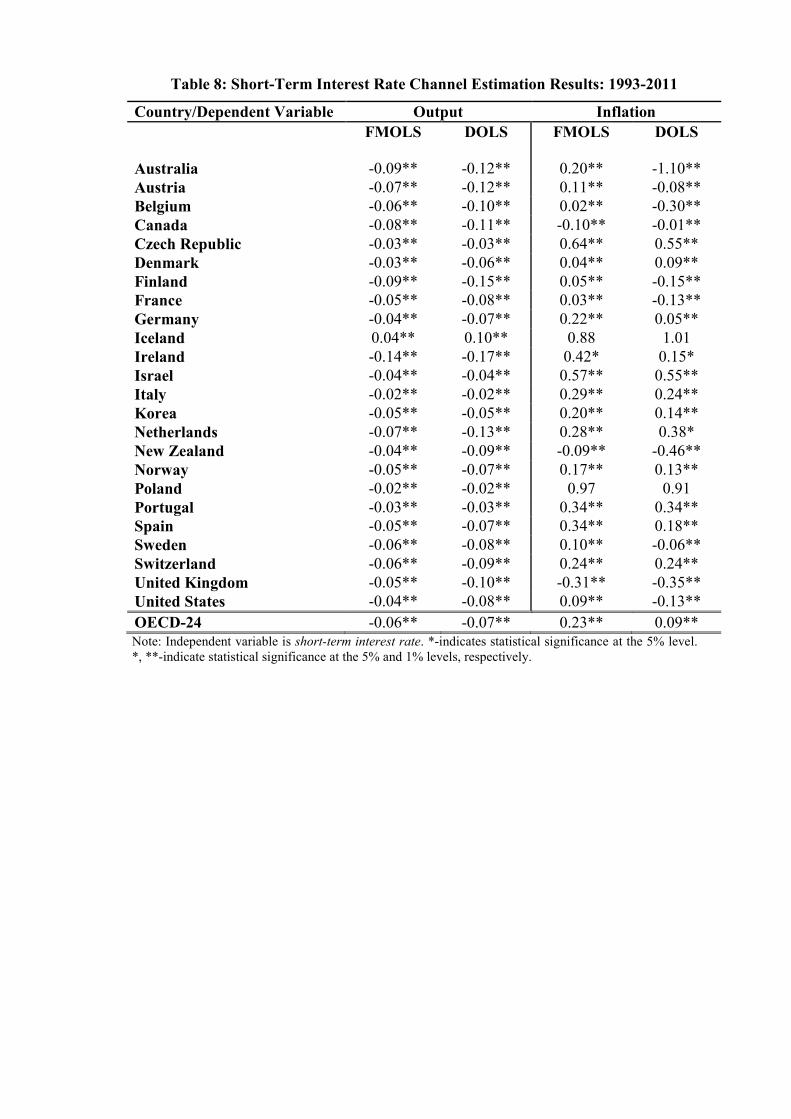
Table 8: Short-Term Interest Rate Channel Estimation Results: 1993-2011

Country/Dependent Variable Output Inflation

FMOLS DOLS FMOLS DOLS

Australia -0.09** -0.12** 0.20** -1.10**

Austria -0.07** -0.12** 0.11** -0.08**

Belgium -0.06** -0.10** 0.02** -0.30**

Canada -0.08** -0.11** -0.10** -0.01**

Czech Republic -0.03** -0.03** 0.64** 0.55**

Denmark -0.03** -0.06** 0.04** 0.09**

Finland -0.09** -0.15** 0.05** -0.15**

France -0.05** -0.08** 0.03** -0.13**

Germany -0.04** -0.07** 0.22** 0.05**

Iceland 0.04** 0.10** 0.88 1.01

Ireland -0.14** -0.17** 0.42* 0.15*

Israel -0.04** -0.04** 0.57** 0.55**

Italy -0.02** -0.02** 0.29** 0.24**

Korea -0.05** -0.05** 0.20** 0.14**

Netherlands -0.07** -0.13** 0.28** 0.38*

New Zealand -0.04** -0.09** -0.09** -0.46**

Norway -0.05** -0.07** 0.17** 0.13**

Poland -0.02** -0.02** 0.97 0.91

Portugal -0.03** -0.03** 0.34** 0.34**

Spain -0.05** -0.07** 0.34** 0.18**

Sweden -0.06** -0.08** 0.10** -0.06**

Switzerland -0.06** -0.09** 0.24** 0.24**

United Kingdom -0.05** -0.10** -0.31** -0.35**

United States -0.04** -0.08** 0.09** -0.13**

OECD-24 -0.06** -0.07** 0.23** 0.09** Note: Independent variable is short-term interest rate. *-indicates statistical significance at the 5% level. *, **-indicate statistical significance at the 5% and 1% levels, respectively.

Table 9: Long-Term Interest Rate Channel Estimation Results: 1994-2011

Country/Dependent Variable Output Inflation

FMOLS DOLS FMOLS DOLS

Australia -0.12** -0.17** 0.20** -0.14**

Austria -0.09** -0.11** -0.08** -0.08**

Belgium -0.08** -0.09** -0.09** 0.03**

Canada -0.09** -0.10** 0.01** 0.14**

Denmark -0.05** -0.05** 0.02** 0.17**

Finland -0.08** -0.10** -0.05** 0.43**

France -0.07** -0.09** 0.00** -0.06**

Germany -0.05** -0.06** -0.02** 0.00**

Iceland -0.02** -0.02** 0.84 0.80

Ireland -0.12** -0.15** -0.34** -1.00**

Italy -0.02** -0.03** 0.38** 0.24**

Japan -0.03** 0.00** 0.26** 0.85

Netherlands -0.10** -0.11** 0.22** 0.51*

New Zealand -0.18** -0.22** -0.44** -0.85**

Norway -0.09** -0.09** 0.12** 0.04**

Portugal -0.03** -0.03** 0.19** 0.15**

Spain -0.06** -0.09** 0.22** -0.05**

Sweden -0.06** -0.09** 0.02** 0.08**

Switzerland -0.11** -0.14** 0.29** 0.01**

United Kingdom -0.09** -0.10** -0.20** -0.35**

United States -0.10** -0.11** 0.11** 0.19**

OECD-22 -0.08** -0.09** 0.04** 0.05** Note: Independent variable is long-term interest rate. *, **-indicate statistical significance at the 5% and 1% levels, respectively.

Table 10: Monetary Channel Estimation Results: 1994-2011

Country/Dependent Variable Output Inflation

FMOLS DOLS FMOLS DOLS

Australia 0.43** 0.44** 0.44 1.66

Canada 0.32** 0.35** 0.30* 0.02

Chile 0.31** 0.32** -1.73** -0.57

Czech Republic 0.32** 0.33** -2.99** -1.82**

Denmark 0.18** 0.17** 0.00** -0.57**

Israel 0.27** 0.28** -3.02** -7.83**

Japan 0.09** 0.07** -0.93** -1.82**

Korea 0.41** 0.40** -1.40** -1.49**

Mexico 0.19** 0.16** -12.58** -1.05

New Zealand 0.34** 0.33** 0.84 1.13

Norway 0.24** 0.23** -0.22** -0.17**

Poland 0.29** 0.28** -6.83** -5.25**

Switzerland 0.29** 0.33** -0.39** 0.27

Turkey 0.10** -0.01** -16.56** -15.62**

United Kingdom 0.27** 0.30** 0.64 0.76

United States 0.52** 0.62* 0.58 0.65

OECD-16 0.29** 0.28** -2.76 -1.30

Note: Independent variable is Narrow Money Index (M1). *, **-indicate statistical significance at the 5% and 1% levels, respectively.

Table 11: Exchange Rate Channel Estimation Results: 1991-2011

Country/Dependent Variable Output Inflation

FMOLS DOLS FMOLS DOLS

Australia -0.38** -0.30** 1.25 2.51

Canada -0.42** -0.41** 0.94 2.49

Czech Republic -0.59** -0.59** 4.46 2.62

Denmark -0.15** -0.14** 0.42 0.63

Hungary 0.19** 0.13** -13.54** -12.23**

Iceland 0.58* 1.04 5.49* 11.47**

Israel 0.59* 0.41** -18.64** -20.04**

Japan -0.19** -0.27** 2.55 0.41

Korea 1.06* 1.05 -4.20** -5.13**

Mexico 0.29** 0.31** -5.60* -6.17*

New Zealand -0.48** -0.51** -2.17* -1.13

Norway -0.26** -0.27** 0.95 0.65

Poland 0.18** -0.06** -28.37** -19.19*

Sweden 0.04** -0.01 -1.81 -1.34

Switzerland -0.43** -0.43** 1.85 1.37

Turkey 0.09** 0.05** -9.88** -4.57*

United Kingdom -0.93** -1.53** -3.23 -5.28*

OECD-17 -0.06** -0.09** -4.17** -3.11

Note: Independent variable is Exchange Rate (NCU/USD). *, **-indicate statistical significance at the 5% and 1% levels, respectively.

Table 12: Wages Channel Estimation Results: 1991-2010

Country/Dependent Variable Output Inflation

FMOLS DOLS FMOLS DOLS

Australia 0.97 0.97 1.82 1.81

Austria 0.79** 0.82** -1.79* -1.85*

Belgium 0.77** 0.81** 0.96 1.36

Canada 0.90 0.91 0.56 0.68

Denmark 0.51** 0.48** 0.11 -0.09

Finland 0.87 0.88* -0.35 0.44

France 0.72** 0.74** -0.41* -0.77*

Germany 0.79** 0.89* -3.79* 3.25

Ireland 1.19** 1.21** 1.35 2.14

Italy 0.43** 0.45** -5.32** -4.62*

Japan -0.59** -0.85** -2.62 -10.37

Korea 0.83** 0.93* -2.66** -2.27*

Luxembourg 1.37** 1.43** 1.21 2.06

Netherlands 0.87* 0.86* -2.56** -2.85**

Norway 0.52** 0.49** -0.05* 0.46

Spain 0.88 0.89 -4.25** -6.94**

Sweden 0.78** 0.84** -1.81* -0.94

Switzerland 2.04** 2.08** -3.67* -2.46*

United Kingdom 0.82** 0.84** -0.92* -0.44

United States 0.83** 0.84** -0.50 -0.85

OECD-20 0.81** 0.83** -1.26** -1.11**

Note: Independent variable is Average Wages. *, **-indicate statistical significance at the 5% and 1% levels, respectively.

Table 13: Credit Channel Estimation Results: 1993-2011

Country/Dependent Variable Output Inflation

FMOLS DOLS FMOLS DOLS

Australia 0.01* 0.01* 0.01* 0.00*

Austria 0.02* 0.02* 0.01* -0.04*

Belgium -0.01* -0.01* -0.01* -0.01*

Czech Republic -0.01* 0.00* 0.23* 0.20*

Denmark 0.00* 0.00* 0.00* 0.00*

Finland 0.01* 0.00* 0.01* 0.00*

France 0.01* 0.01* 0.00* -0.02*

Germany 0.00* 0.00* -0.04* -0.01*

Iceland 0.00* 0.00* 0.03* 0.03*

Ireland 0.00* 0.00* -0.01* -0.02*

Israel 0.03* 0.03* -0.13* -0.32*

Italy 0.00* 0.00* 0.00* 0.02*

Korea 0.01* 0.01* -0.04* -0.03*

Spain 0.00* 0.00* -0.01* -0.03*

Sweden 0.00* 0.00* 0.01* 0.00*

Switzerland 0.01* 0.01* -0.02* -0.02*

United Kingdom 0.00* 0.00* 0.02* 0.01*

United States 0.01* 0.01* 0.00* -0.01*

Netherlands 0.00* 0.00* -0.01* 0.00*

New Zealand 0.01* 0.01* 0.02* 0.01*

Poland 0.02* 0.01* -0.26* -0.17*

Portugal 0.00* 0.00* -0.01* -0.02*

OECD-22 0.02* 0.02* -0.01* -0.02* Note: Independent variable is Bank-sector Credit. *-indicates statistical significance at the 1% level.

Table 14: Post-Estimation Test of Transmission Heterogeneity

Channel Dependent

Variable FMOLS DOLS

IMIR Chi-Squared P-value Chi-Squared P-value

GDP 235.43 0.00 220.88 0.00

CPI 301.94 0.00 288.38 0.00

STIR

GDP 175.15 0.00 147.78 0.00

CPI 140.51 0.00 135.25 0.00

LRIR

GDP 284.00 0.00 323.36 0.00

CPI 107.00 0.00 118.07 0.00

ER

GDP 78.00 0.00 78.52 0.00

CPI 133.84 0.00 110.88 0.00

M1

GDP 803.74 0.00 462.46 0.00

CPI 230.00 0.00 48.00 0.00

WG

GDP 436.33 0.00 798.29 0.00

CPI 56.08 0.00 49.72 0.00

CR

GDP 672.37 0.00 1110.81 0.00

CPI 61.12 0.00 60.17 0.00 Note: Null hypothesis is parameter homogeneity. P-values of zero indicate rejection of the hypothesis of homogeneous monetary response parameters.