cross-national comparative research with longitudinal data: understanding youth poverty maria...
TRANSCRIPT

Cross-national comparative research with longitudinal data:
Understanding youth poverty
Maria Iacovou (ISER)with
Arnstein Aassve, Maria Davia, Letizia Mencarini, Stefano Mazzucco
Funded by JRF as part of the Poverty among Youth: International Lesson for the UK project, under LOOP programme

Comparative research at ISER
• Big EU-funded programmes – EPAG, DYNSOC, ESEC
• EUROMOD – Tax & benefits microsimulation
• Lots of stand-alone projects, PhDs, etc. • Data
– ECHP, EU-SILC, ESS
• Life chances and living standards (ESRC)– Incomes, work and families, methodology– Combines micro-level analysis and microsimulation– Enlarged EU
• Youth poverty (JRF funded)– http://www.jrf.org.uk/bookshop/details.asp?pubID=922

Overview of youth poverty programme
• Descriptive paper– tabulating youth poverty rates across Europe
• Explaining poverty and poverty transitions– characteristics and events associated with poverty
• Addressing issues of causality– Does moving out of the parental home “cause” you to be poor, or are
young people who are likely to be poor more likely to leave home?
• Intra-household support– Looking at young people who live with their parents, and classifying
them according to who supports whom in the household.
• Don’t expect much detail. Household/family used interchangeably.

Motivation
• Vulnerability– Unemployment, homelessness, criminality and incarceration,
drug abuse, mental health problems, etc etc
• Lack of research into youth poverty– Lots of research for other vulnerable groups
• Comparative aspect– Increasing body of knowledge on variations within EU– Do patterns of youth poverty mirror trends among the general
population?

Data
• European Community Household Panel
• Exclude Sweden and Luxembourg (so 13 countries)
• 8 waves 1994 - 2001
• Young people aged 17-35
Computing incomes• Use personal income data from year t+1 (which relates to year t) for each
individual present in the household in year t
• If one individual in the household has missing data at year t+1, impute their income at t+1 using income at year t.
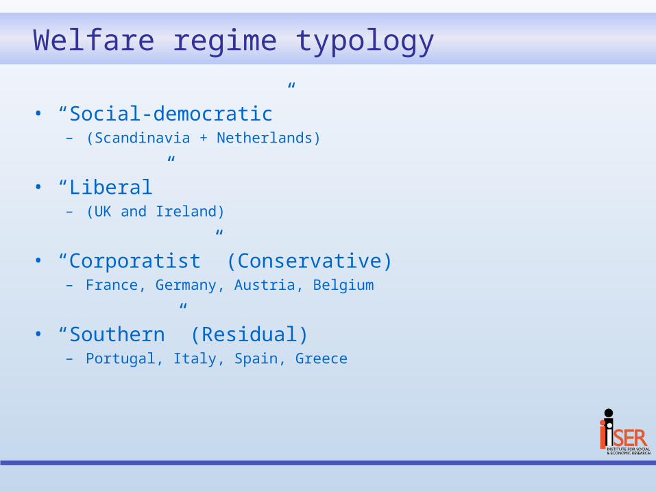
Welfare regime typology
• “Social-democratic” – (Scandinavia + Netherlands)
• “Liberal” – (UK and Ireland)
• “Corporatist” (Conservative)– France, Germany, Austria, Belgium
• “Southern” (Residual)– Portugal, Italy, Spain, Greece

Poverty, by age: UK
0%
10%
20%
30%
40%
0 10 20 30 40 50 60 70
Age
% p
oo
r (i
nco
me
un
der
60%
med
ian
)

Social-democratic regimes
0%
10%
20%
30%
40%
0 10 20 30 40 50 60 70
Age
% p
oo
r (i
nco
me
un
der
60%
med
ian
)
Finland Denmark Netherlands UK

“Conservative” regimes
0%
10%
20%
30%
40%
0 10 20 30 40 50 60 70
Age
% p
oo
r (i
nco
me
un
der
60%
med
ian
)
UK France Germany
Austria Belgium

Southern regimes
0%
10%
20%
30%
40%
0 10 20 30 40 50 60 70Age
% p
oor (inco
me
under
60%
med
ian)
UK Portugal Spain
Italy Greece
Ireland

What young people are at greatest risk?
0%
20%
40%
60%
80%
100%
. FIN DEN NETH UK IRE FRA GER AUS BEL POR SPA ITA GRE
Social Democratic Liberal Corporatist Southern
Left parental home Still in parental home
• 3 age groups: 16-19, 20-24, 25-29
• Poverty risk reduces with age, and is increased on leaving home

Leaving home and poverty
POR
SPA
GRE BEL
ITA
AUS
FRA
GER
IRE
UK
DEN
NETFIN
0%
10%
20%
30%
40%
50%
60%
70%
0% 10% 20% 30% 40% 50%
Difference between poverty rates of young people who have left home and those living at home
(20-24-year-olds)
% o
f th
os
e a
ge
d 2
0-2
4 w
ho
ha
ve
le
ft t
he
p
are
nta
l h
om
eA bit of a puzzle

Multivariate analysis
• Cross-sectional – who is poor (and deprived)– Pooled sample across waves– Controls: age, sex, employment/unemployment/studying, living
arrangements, marital status, number of children
• Entry into & exit from poverty (and deprivation)– Pairs of individuals present in sample in t and t+1– Longitudinal – who becomes poor (or deprived)– Also control for events: moving out of the parental home,
having a baby, etc.
• In all cases– Probit regressions for poverty, linear models for deprivation– Control for multiple observations– Marginal effects reported

Results from multivariate analysis
Poverty incidence
-0.2
-0.1
0
0.1
0.2
0.3
FIN DEN NET UK IRE FRA GER AUS BEL POR SPA ITA GRE
Non employed
Not in education
Left parental home

More results
Poverty incidence
-0.2
-0.1
0
0.1
0.2
0.3
FIN DEN NET UK IRE FRA GER AUS BEL POR SPA ITA GRE
Married
Cohabiting
Number of children
• Moving swiftly onwards
• Deprivation

Poverty entry
-0.1
-0.05
0
0.05
0.1
0.15
0.2
FIN DEN NET UK IRE FRA GER AUS BEL POR SPA ITA GRE
Left parental homeJust left parental homeHas childrenNew children last year

More on poverty entry
-0.1
-0.05
0
0.05
0.1
0.15
0.2
FIN DEN NET UK IRE FRA GER AUS BEL POR SPA ITA GRE
MarriedJust marriedCohabiting Just started cohabiting

Exits from poverty
-0.5
-0.4
-0.3
-0.2
-0.1
0
0.1
FIN DEN NET UK IRE FRA GER AUS BEL POR SPA ITA GRE
Left parental homeJust left parental homeHas childrenNew children last year

More on poverty exits
-0.3
-0.2
-0.1
0
0.1
0.2
0.3
FIN DEN NET UK IRE FRA GER AUS BEL POR SPA ITA GRE
Employed Recently employedNot in education Just finished education

Does leaving home “cause” poverty?
• Or is it a selection effect?– do we just observe higher levels of poverty among those who
have left home, because those at higher risk of poverty are more likely to leave home at younger ages?
• Possibly a bit of both?

Propensity score matching
• We want to compare risk of poverty in two situations– Remaining in the parental home, and living independently
• For obvious reasons, we can’t do this for individuals– No “counterfactual”
– “Match” individuals who are identical in all observable characteristics, except living arrangements
• Not without problems– Some people can’t be matched– Oldest Scandinavians; youngest Southern Europeans– “Common support” problem
• Importance of longitudinal data

PSM procedure
• Identify “treatment” and “control” groups – those who did and did not leave home
• For both groups: synthesise counterfactuals– We use up to three “near neighbours”
• Average treatment effect on the treated (ATT)– Start with treatment group and synthesise counterfactuals– ATT = poverty rate in treatment gp less rate in control gp– For those who did leave home: The extra risk of entering
poverty arising from leaving home.
• Average treatment effect on the control (ATC)– For those who did not leave home: The extra risk of entering
poverty which would have arisen if they had left home

ATT estimates
0
0.1
0.2
0.3
0.4
0.5
0.6
FIN DEN NET UK IRE FRA GER AT BEL PT ES ITA GRE
descriptive
PSM

ATT estimates
0
0.1
0.2
0.3
0.4
0.5
0.6
FIN DEN NET UK IRE FRA GER AT BEL PT ES ITA GRE
descriptive
PSM
– Significant selection effects– Young people who are most likely to experience
poverty if they leave home …… are actually more likely to remain at home.
– Analysis ignoring this underestimates effect of leaving home.

ATC against ATT 25-29
GRE
PT
IRE
ES
GER
FRITA
AT
0
0.02
0.04
0.06
0.08
0.1
0.12
0.14
0 0.02 0.04 0.06 0.08 0.1 0.12 0.14
ATC
AT
TEffects on treatment and control
• Rational in so far as those who are at higher risk of poverty are more likely to remain at home – except in Finland and Denmark.
• But we haven’t uncovered a “rational” reason for the huge differences between countries.

Conclusions
• Young people are at generally high risk of poverty
• Leaving home is the most important trigger
• Having children and being unemployed are also risk factors

Policy conclusions
• Child poverty measures– also reduce poverty among young adults still living at home.
• Financial assistance – in first year or two of living away from the parental home.
• Scandinavian systems of support for young parents– family support plus family-friendly labour markets.
• Austrian and German style paid apprenticeships– effective in keeping youth poverty rates extremely low.
• Employment plays a part in reducing youth poverty – but getting a job is not enough; keeping a job is important too.

the end

Including Ireland…
0%
10%
20%
30%
40%
0 10 20 30 40 50 60 70Age
% p
oor (inco
me
under
60%
med
ian)
UK Ireland Spain
back