cross-covariance-based model reduction
TRANSCRIPT

Cross-Covariance-Based Model ReductionP. Benner, S. Grundel, C. Himpe
Max Planck Institute MagdeburgComputational Methods in System and Control Theory Group
Simulation of Energy Systems Team
MS28 – Model Reduction Methods for Simulation and (Optimal) ControlENUMATH – European Conference on Numerical Mathematics
2017–09–26

MotivationMathematically:
Many-query large-scale nonlinear input-output system.
Use data-driven nonlinear model reduction.
Transfer concepts from linear systems.
Reuse results from system theory,
based on empirical balancing1.
Practically:
Repeated simulation of gas transportation networks.
Transient behaviour on typical temporal resolutions.
Test families of possible supply-demand scenarios.
Uncertainty quantification for unsteady supply.
Short-term dispatch forecasts.1
C. H. Combined State and Parameter Reduction for Nonlinear Systems with an Application in Neuroscience.Westfalische Wilhelms Universitat Munster, 2016.
C. Himpe, [email protected] Cross-Covariance-Based Model Reduction 2/25

MathEnergy Project
MathEnergy:
Mathematical Key Technologies for Evolving Energy Grids.
Partners:
Fraunhofer SCAI
Fraunhofer ITWM
Max Planck Institute Magdeburg (Sub-Project: Model Reduction)
Technische Universitat Berlin
Technische Universitat Dortmund
Humboldt Universitat zu Berlin
Friedrich-Alexander Universitat Erlangen-Nurnberg
PSI AG
Funding:
German Federal Ministry for Economic Affairs and Energy (BMWi)
C. Himpe, [email protected] Cross-Covariance-Based Model Reduction 3/25

Gas Transport Pipeline
Input:
Pressure @ Inlet (Supply)
Mass-Flux @ Outlet (Demand)
Output:
Mass-Flux @ Inlet (Supply)
Pressure @ Outlet (Demand)
C. Himpe, [email protected] Cross-Covariance-Based Model Reduction 4/25

Euler Equations
1D Isothermal Euler Equation2:
1
γ0
∂
∂tp = −
( z0(p)2
z0(p)− pz′0(p)
) 1
S
∂
∂xq,
1
S
∂
∂tq = − ∂
∂xp − γ0
S2
∂
∂x
q2z0(p)
p︸ ︷︷ ︸Inertia Term
− g
γ0
p
z0(p)
∂
∂xh︸ ︷︷ ︸
Gravity Term
−λ(q)γ02DS2
z0(p)q|q|p︸ ︷︷ ︸
Friction Term
Average pressure / mass-flux over pipe cross-section area.
Conservation of momentum / mass
Hyperbolic (coupled transport)
Nonlinear (friction term)
Additional nonlinearities (compressibility)2
S. Grundel, N. Hornung, B. Klaassen, P. Benner and T. Clees. Computing Surrogates for Gas Network Simulation UsingModel Order Reduction. In: Surrogate-Based Modeling and Optimization, Applications in Engineering: 189–212, 2013.
C. Himpe, [email protected] Cross-Covariance-Based Model Reduction 5/25

Semi-Discretized Model
Spatial Discretization and Index Reduction3,4:(E1 00 1
)(phqh
)=
(0 A1
A2 0
)(phqh
)+
(fp(ph, up)
fq(ph, qh, up)
)+
(0 B1
B2 0
)(upuq
)(ypyq
)=
(C1 00 C2
)(phqh
)Descriptor system,
Index-1 differential-algebraic equation (DAE).
Analytic index reduction to index-0 → implicit ODE.
3S. Grundel, L. Jansen, N. Hornung, T. Clees, C. Tischendorf and P. Benner. Model Order Reduction of Differential
Algebraic Equations Arising from the Simulation of Gas Transport Networks. In: Progress in Differential-Algebraic Equations,Differential Equation Forum: 183–205, 2014.
4S. Grundel, N. Hornung and S. Roggendorf. Numerical Aspects of Model Order Reduction for Gas Transportation
Networks. In: Simulation-Driven Modeling and Optimization: 1–28, 2016.
C. Himpe, [email protected] Cross-Covariance-Based Model Reduction 6/25

Gas Pipeline Input-Output System
Abstract Input-Output System:(Epphqh
)=
(fp(ph, qh, up, uq)fq(ph, qh, up, uq)
)(ypyq
)=
(gp(ph)gq(qh)
)Supply pressure up(t) := p(0, t)
Demand mass-flux uq(t) := q(L, t)
Demand pressure yp(t) := p(L, t)
Supply mass-flux yq(t) := q(0, t)
C. Himpe, [email protected] Cross-Covariance-Based Model Reduction 7/25

Target / Actual
Target:
1. Find reduced order model,
2. approximating input-output behaviour,
3. without linearization.
Actual:
Coupling (Pressure / Mass-flux)
Nonlinear (Friction / Compressibility)
Hyperbolicity
C. Himpe, [email protected] Cross-Covariance-Based Model Reduction 8/25

Cross-Covariance
Cross-Covariance:
XC(τ) :=
∫ ∞0
F (t)G∗(τ + t) dt
τ is the lag between F and G.
Matrix of pair-wise shifted co-movement indices.
Normalize to obtain cross-correlation.
C. Himpe, [email protected] Cross-Covariance-Based Model Reduction 9/25

State-Output Co-Movement
State-Output Cross-Covariance with zero lag (τ ≡ 0):
XC =
∫ ∞0
x(t; u)︸ ︷︷ ︸F
[yᵀ(t; x0,1), . . . , yᵀ(t; x0,N)]︸ ︷︷ ︸
G∗
dt
SISO System: dim(u(t)) = dim(y(t)) = 1
x(t; u) perturbed input state trajectory
y(t; x0,i) perturbed i-th initial state output trajectory
Input-to-state and state-to-output mappings
identify input-output behaviour.
C. Himpe, [email protected] Cross-Covariance-Based Model Reduction 10/25

Linear State-Output Co-Movement
Linear SISO System:
x(t) = Ax(t) + bu(t)
y(t) = cx(t)
State-Output cross-covariance with unit perturbance:
XC(0) =
∫ ∞0
(eAt b1)(c eAt 1) dt =
∫ ∞0
(eAt b)(c eAt) dt
⇒ AXC +XCA = −bc
C. Himpe, [email protected] Cross-Covariance-Based Model Reduction 11/25

A Quick Example
Linear SISO System:
x(t) =
−1 0 00 −1 00 0 −1
x(t) +
101
u(t)
y(t) =(
0 1 1)x(t)
Associated Cross-Covariance Matrix:
XC =
0 12
12
0 0 00 1
212
C. Himpe, [email protected] Cross-Covariance-Based Model Reduction 12/25

From Linear to Nonlinear
Interpretation:
SISO: State-Output Co-Movement
Square MIMO: Input-Average State-Output Co-Movement
MIMO: Input-Output-Average State-Output Co-Movement
Nonlinear:
Instead of a closed form (for the impulse response)
we have to use simulated or measured data.
→ Approximate nonlinear cross-covariance by data-driven approach5.
5J. Hahn and T.F. Edgar. Balancing Approach to Minimal Realization and Model Reduction of Stable Nonlinear
Systems. Industrial & Engineering Chemical Research, 41(9): 2204–2212, 2002.
C. Himpe, [email protected] Cross-Covariance-Based Model Reduction 13/25

Cross-Covariance Computation
Empirical Cross Covariance Matrix6 (square systems):
XC :=M∑
m=1
∫ ∞0
Ψm(t) dt ∈ RN×N
Ψmij (t) = (xmi (t)− xmi )(yjm(t)− yjm) ∈ R
Empirical Cross Covariance Matrix7 (non-square systems):
Xc :=
Q∑q=1
M∑m=1
∫ ∞0
Ψm(t) dt ∈ RN×N
Ψmij (t) = (xmi (t)− xmi )(yjq(t)− yjq) ∈ R
6C. H. and M. Ohlberger. Cross-Gramian Based Combined State and Parameter Reduction for Large-Scale Control
Systems. Mathematical Problems in Engineering, 2014:1–13, 2014.7
C. H. and M. Ohlberger. A note on the cross Gramian for non-symmetric systems. System Science and ControlEngineering, 4(1): 199–208, 2016.
C. Himpe, [email protected] Cross-Covariance-Based Model Reduction 14/25

Model Order Reduction
Reduced Order Input-Output (Descriptor) System:
Ex(t) = f(x(t), u(t))
y(t) = g(x(t), u(t))
}MOR→
{Erxr(t) = fr(xr(t), u(t))
y(t) = gr(xr(t), u(t))
u 7→ x 7→ y
dim(u(t))� dim(x(t))
dim(y(t))� dim(x(t))
dim(xr(t))� dim(x(t))
‖y − y‖ � 1
C. Himpe, [email protected] Cross-Covariance-Based Model Reduction 15/25

Projection-Based Model Reduction
Projection-Based Reduced Order Model:
(V1EU1)xr(t) = V1f(U1xr(t), u(t))
y(t) = g(U1xr(t), u(t))
Approximation: xr := V1x(t)→ x(t) ≈ U1xr(t)
Reducing truncated projection: V1
Reconstructing truncated projection: U1
Bi-Orthogonality: V1U1 = 1
Task: Find U1, V1
C. Himpe, [email protected] Cross-Covariance-Based Model Reduction 16/25

Cross-Covariance-Based Model Reduction
Singular Value Decomposition:
XCSVD= UDV
Projections from Cross-Covariance based on Dii:
W.l.o.g. σi = Dii sorted descendingly.
U∗(1...n), V(1...n)∗ are left and right principal directions.
Reconstrucing projection: U =(U1 U2
)Galerkin reducing projection: V1 = Uᵀ
1
Petrov-Galerkin reducing projection8: V =(V1 V2
)8
D.C. Sorensen and A.C. Antoulas. The Sylvester equation and approximate balanced reduction. Linear Algebra and itsApplications, 351–352: 671–700, 2002.
C. Himpe, [email protected] Cross-Covariance-Based Model Reduction 17/25

Structured Affine ReductionCross-Covariance Structure for Gas Transport:
XC =
(XC,pp XC,pq
XC,qp XC,qq
)Structured Reduced Order Model9:(
(VpEpUp)prqr
)=
(Vpfp(p+ Uppr, q + Uqxq, up, uq)Vqfq(p+ Uppr, q + Uqqr, up, uq)
)(ypyq
)=
(gp(p+ Uppr)gq(q + Uqqr)
)Pipe is a coupled square MIMO system: 2 inputs and 2 outputs.
Center pressure and mass-flux around steady state p, q.
Only Perturbation training!9
H. Sandberg and R.M. Murray. Model reduction of interconnected linear systems. Optimal Control Applications andMethods, 30(3): 225–245, 2009.
C. Himpe, [email protected] Cross-Covariance-Based Model Reduction 18/25
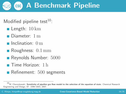
A Benchmark Pipeline
Modified pipeline test10:
Length: 10 km
Diameter: 1 m
Inclination: 0 m
Roughness: 0.1 mm
Reynolds Number: 5000
Time Horizon: 1 h
Refinement: 500 segments
10M. Chaczykowski. Sensitivity of pipeline gas flow model to the selection of the equation of state. Chemical Research
Engineering and Design, 87: 1596–1603, 2007.
C. Himpe, [email protected] Cross-Covariance-Based Model Reduction 19/25

A Scenario
0 1000 2000 3000-1
-0.5
0
0.5
1
Pre
ssure
@ S
upply
Node(s
)
0 1000 2000 3000-10
-5
0
5
10
Mass F
low
@ D
em
and N
ode(s
)
0 1000 2000 300050
55
60
65
70
75
Mass F
low
@ S
upply
Node(s
)
0 1000 2000 300069.84
69.86
69.88
69.9
69.92
69.94
Pre
ssure
@ D
em
and N
ode(s
)
Figure: Supply pressure, demand mass-flux, supply mass-flux and demand pressure.
C. Himpe, [email protected] Cross-Covariance-Based Model Reduction 20/25

emgr - EMpirical GRamian Framework (Version: 5.2)
Empirical Gramians:
Empirical Controllability GramianEmpirical Observability GramianEmpirical Linear Cross GramianEmpirical Cross Gramian?
Empirical Sensitivity GramianEmpirical Identifiability GramianEmpirical Joint Gramian
Features:
Interfaces for: Solver, inner product kernels & distributed memoryNon-Symmetric option for all cross GramiansCompatible with OCTAVE and MATLABVectorized and parallelizableOpen-source licensedFunctional design
More info: http://gramian.de
C. Himpe, [email protected] Cross-Covariance-Based Model Reduction 21/25

Model Reduction Error
100 200 300 400 500 600 700 800 900
State Dimension
10 -15
10 -10
10 -5
10 0
Rela
tive O
utp
ut E
rror
Empirical Square Cross-Covariance (Unstructured)
Empirical Square Cross-Covariance (Structured)
Empirical Non-Square Cross-Covariance (Unstructured)
Empirical Non-Square Cross-Covariance (Structured)
Figure: Relative L2 model reduction error for the benchmark pipeline.
C. Himpe, [email protected] Cross-Covariance-Based Model Reduction 22/25
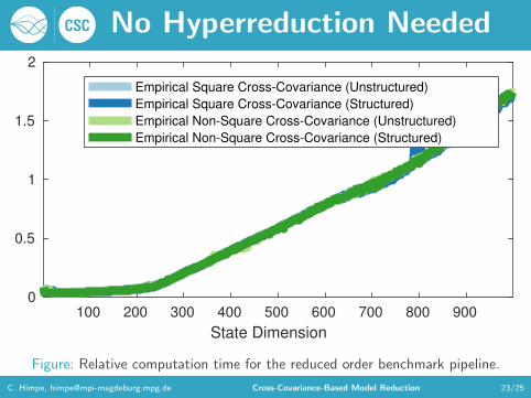
No Hyperreduction Needed
100 200 300 400 500 600 700 800 900
State Dimension
0
0.5
1
1.5
2
Empirical Square Cross-Covariance (Unstructured)
Empirical Square Cross-Covariance (Structured)
Empirical Non-Square Cross-Covariance (Unstructured)
Empirical Non-Square Cross-Covariance (Structured)
Figure: Relative computation time for the reduced order benchmark pipeline.
C. Himpe, [email protected] Cross-Covariance-Based Model Reduction 23/25

Outlook
From Pipelines to Pipe Networks:
Repetitive modelling11.
Conservation of mass in all nodes.
Conservation of energy in all nodes.
Up Next:
Large complex networks
Include compressors
Include valves
Per-pipe parameters
Power grid / gas net coupling
11T.P. Azevedo-Perdicoulis and G. Jank. Modelling Aspects of Describing a Gas Network Through a DAE System. IFAC
Proceedings Volume, 40(20): 40–45, 2007.
C. Himpe, [email protected] Cross-Covariance-Based Model Reduction 24/25

Summary
Gas Transport in Pipelines: Isothermal Euler equations.
System-theoretic: Balancing controllability and observability.
Nonlinear cross-covariance: Empirical cross Gramian matrix.
http://mathenergy.de
http://himpe.science
Acknowledgment:Supported by the German Federal Ministry for Economic Affairs andEnergy, in the joint project: “MathEnergy – Mathematical KeyTechnologies for Evolving Energy Grids”, sub-project: Model OrderReduction (Grant number: 0324019B).
C. Himpe, [email protected] Cross-Covariance-Based Model Reduction 25/25