CROP PRODUCTION AND SOIL SALINITY: EVALUATION OF FIELD DATA FROM INDIA BY SEGMENTED LINEAR REGRESSION WITH BREAKPOINT

R.J. Oosterbaan 1), D.P. Sharma 2), K.N. Singh 2) and K.V.G.K Rao 2)

1) International Institute for Land Reclamation and Improvement/ILRI, Wageningen, The Netherlands2)Central Soil Salinity Research Institute/CSSRI, Karnal, Haryana, India

Paper published in Proceedings of the Symposium on Land Drainage for Salinity Control in Arid and Semi-Arid Regions, February 25th to March 2nd, 1990, Cairo, Egypt, Vol. 3, Session V, p. 373 - 383

Copy on web-site www.waterlog.info/segreg.htm

AbstractA graphic plot of field data on crop production versus production factors, e.g. soil salinity, usually shows considerable scatter. The scatter is due to the presence of many production factors in agriculture, which cannot be all accounted for. However, if the production factor considered has a significant influence on crop yield, it should be possible to detect a relation between the yield and the production factor, despite of the scatter. Then, statistical methods need to be applied to perform a confidence analysis of the relation found and of its parameters.

If the analysis reveals that the relation is dependable, it would be possible to predict the yield response to changes in the growth factor considered, e.g. upon soil reclamation. If, on the other hand there is no dependability, one can conclude that there must be other production factors involved that have far greater influence on the yield than the factor considered. It would the be possible to adjust the research objectives and investigate more significant factors explaining the yields.

This article discusses the segmented linear (broken-line) regression with a break-point of the yield of barley, mustard and wheat on soil salinity. By this method the data are separated into two groups according to the value of the salinity. Such an analysis permits the determination of the critical or threshold value of the soil salinity, beyond which the yields arenegatively affected, the degree to which the soil salinity explains the variation in yields, the yield decline per unit increase of soil salinity, and the yield benefit to be expected from a salinity control program under farmers' conditions.

The data were collected during 1987 and 1988 in the Sampla pilot area by the Central Soil Salinity Research Institute, Karnal, Haryana, India.

Key-wordsBroken-line regression, segmented linear regression, break-point, crop yield, crop production,production function, barley, mustard, wheat, India, soil salinity, threshold value, critical value.

NoteOn page 11 and following new developments after publication of this article are added in three addendums.

1

Introduction

The relation between crop production and soil salinity is often derived from controlled experiments in laboratories, pot experiments, lysimeter studies or experimental fields (ref. 3), where all growth factors, except the factor under study, are maintained constant, often at optimum level. Under farmers' and field conditions, however, the growth conditions are quite variable so that, by interaction of the factors, the relations need not be the same and anyway, they are subject to a large degree of variation. Examples of such relations were given by Oosterbaan (ref. 4) and Nijland and El Guindy (ref. 1).

To determine the relation between crop production and salinity in an agricultural area and to assess the extent and degree of salinity problems, it deserve recommendation to implement field surveys sampling crop yield and soil salinity at random, and perform an appropriate statistical regression analysis of the data obtained.

Nijland and El Guindy (ref. 2) have presented a method of sequential regression analysis of crop yield on two production factors, using linear regression equations whereby the values of both factors are divided into two groups containing respectively values smaller and larger than a critical or threshold value (the break-point). Thus, the two-dimensional non-linear multiple regression is simplified to a four-fold (segmented) one-dimensional linear regression. The advantage of this linearization is that:1. The commonly known principles of the one-dimensional linear regression analysis can

be applied;2. The latter analysis, as well as the corresponding analysis of confidence intervals of the

various parameters involved is relatively simple;3. Critical or threshold values can be established;4. The relative influence of the two production factors, as well the effect of their degree

of correlation, can be readily assessed.Due to the usual presence of scatter, the introduction of non-linear instead of linear regressionwould not result in better-fitting equations.

Crop Yields and soil salinity in Sampla, Haryana, India

Figures 1, 2 and 3 show the results of measurements of crop yield (barley, mustard and wheat respectively) and soil salinity in the Sampla pilot area, Haryana, India. The soil salinity is represented by the electric conductivity of an extract of a saturated soil paste (ECe), with a soil sampling depth over the top 30 cm. The crop yield was determined in sample plots of 5m x 10m, and the ECe values are an average of 3 samples per plot. All measurements were madeat harvest date in the years 1987 and 1988. The data were collected by the Central Soil Salinity Research Institute, Karnal, Haryana, India.

The figures show that the relation between yield and salinity is catterd, but the envelope curves in the figures indicate that there exists a critical (or threshold) value of soil salinity below which the yield is not affected by the salinity, whereas beyond this value the yield decreases with increasing salinity. The production function can therefore be described by two straight lines, of which the first is horizontal and extends up to the threshold, and the second is descending from the threshold onwards. The threshold, therefore, is a break-point.

2

3

Method of statistical analysis

The general expression for the production function can be written as:

Y = Ys + V [ECe < B] (Eq. 1)

Y = Ag(S-Sg) + Yg +V [ECe > B] (Eq. 2)

where:

Y is the crop productionS is the soil salinity (ECe)B is the break-point of salinityYs is the average crop production for data with S<BAg is the slope of the production function for data with S>BSg is the average soil salinity for data with S>BYg is the average crop production for data with S>BV is the random variation

The slope Ag is determined from:

Ag = (Ys-Yg)/(B-Sg) (Eq. 3)

4

The most likely value of the threshold can be found by assuming a range of break-points and choosing the point with the klargest coefficient of explanation (Ce, in literature often denoted by R2) defined by:

Ce = 1 - MSD/Dt2 (Eq. 4)

where:

Dt is the standard deviation of all yield data taken with respect to their mean MSD is the mean squared deviation of the yield from the production function Eq. 1&2

and:

MSD = (Ng.Dp2 + Ns.Ds2)/Nt (Eq. 5)

where:

Dp is the standard deviation of the yield data with S>B, taken with respect to the expected value of the yield according to the production function Eq. 2Ng is the number of data with S>B Ds is the standard deviation of the yield data with S<B taken with respect to the mean value YsNs is the number of data with S<BNt is the total number of data

If the harvested plots represent a random sample of the area investigated, the proportion of data with salinity below and above its threshold gives an indication of the area fraction affected by salinity problems. In addition, statements can be formulated about the severity of the salinity problem in the affected area. Also, the yield benefit obtainable from a salinity reclamation program can be estimated.

When the most likely break-point has been found, confidence statements can be made about the slope Ag of the production function and the potential yield increase using standard statistical techniques. Thus the standard deviation of Ag is found from:

Da = Dp/(De.√N') (Eq. 6)

where:

Dp is the standard deviation of the yield data with S>B, taken with respect to the expected value of the yield according to the production function Eq. 2De is the standard deviation of the salinity data with S>BN' is the number of data with S>B less 2

The intersection point, where S=B, of the lines given by Eq. 1 and 2 is:

B = Sg + (Ys-Yg)/Ag

Setting F = Ys-Yg , X = 1/Ag, and Z = F.X the former equation becomes

B = Sg + F.X = Sg + Z

5

The standard error of B can now be found from the principle of propagation of errors in an addition of uncorrelated magnitudes subject to random variation as:

Eb2 = Ee2 + Ez2 (Eq. 7)

where :

Ee is the standard error of the average salinity with S>BEz is the standard error of Z

and:

Ee = De/√Ng (Eq. 8)

Ez2 = F2.Ex2 + X2.Ef2 (Eq. 9)

where:

Ex is the standard error of X=1/Ag

Ef is the standard error of F=Ys-Yg

The value of Ex in Eq. 9 is calculated from the error of inverse magnitudes as:

Ex = Da/Ag2 (Eq. 10)

where Da is the standard deviation of Ag (Eq. 6)

The value of Ef in Eq. 9 is found from:

Ef2 = Es2 + Eg2 = Ds2/Ns + Dg2/Ng (Eq.11)

where:

Es = the standard error of the average Ys [S<B] = Ds/√Ns

Eg is the standard error of the average Yg [S>B] = Dg/√Ng

With the above set equations the standard error of break-point B can be determined.

Results of segmented linear regression

The results of the segmented linear regression performed on the data shown in the figures are given in Table 1. From these data, using Eq. 1 and 2, the following crop production functions of soil salinity can be derived:

6

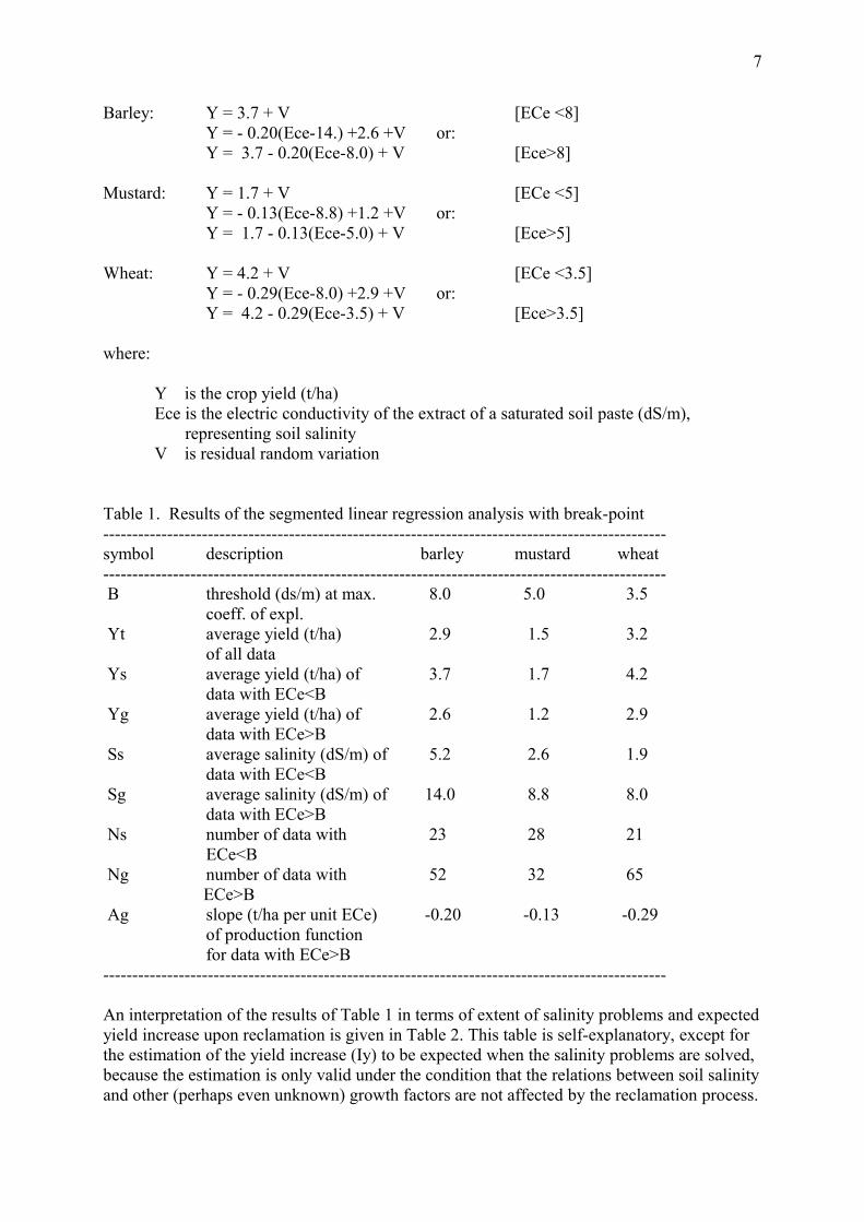
Barley: Y = 3.7 + V [ECe <8]Y = - 0.20(Ece-14.) +2.6 +V or: Y = 3.7 - 0.20(Ece-8.0) + V [Ece>8]

Mustard: Y = 1.7 + V [ECe <5]Y = - 0.13(Ece-8.8) +1.2 +V or: Y = 1.7 - 0.13(Ece-5.0) + V [Ece>5]

Wheat: Y = 4.2 + V [ECe <3.5]Y = - 0.29(Ece-8.0) +2.9 +V or: Y = 4.2 - 0.29(Ece-3.5) + V [Ece>3.5]

where:

Y is the crop yield (t/ha)Ece is the electric conductivity of the extract of a saturated soil paste (dS/m), representing soil salinityV is residual random variation

Table 1. Results of the segmented linear regression analysis with break-point-------------------------------------------------------------------------------------------------symbol description barley mustard wheat------------------------------------------------------------------------------------------------- B threshold (ds/m) at max. 8.0 5.0 3.5

coeff. of expl. Yt average yield (t/ha) 2.9 1.5 3.2

of all data Ys average yield (t/ha) of 3.7 1.7 4.2

data with ECe<B Yg average yield (t/ha) of 2.6 1.2 2.9

data with ECe>B Ss average salinity (dS/m) of 5.2 2.6 1.9

data with ECe<B Sg average salinity (dS/m) of 14.0 8.8 8.0

data with ECe>B Ns number of data with 23 28 21

ECe<B Ng number of data with 52 32 65 ECe>B Ag slope (t/ha per unit ECe) -0.20 -0.13 -0.29

of production functionfor data with ECe>B

-------------------------------------------------------------------------------------------------

An interpretation of the results of Table 1 in terms of extent of salinity problems and expectedyield increase upon reclamation is given in Table 2. This table is self-explanatory, except for the estimation of the yield increase (Iy) to be expected when the salinity problems are solved, because the estimation is only valid under the condition that the relations between soil salinityand other (perhaps even unknown) growth factors are not affected by the reclamation process.

7

Table 2. Interpretation of results of Table 1.-------------------------------------------------------------------------------------------------symbol description barley mustard wheat------------------------------------------------------------------------------------------------- Pp percentage salinity problems 69 53 76

Pp = 100 Ng/(Ng+Ns) Iy potential average yield 0.8 0.2 1.0 increase (t/ha) : Iy = Ys-Yt PIy percentage yield increase 28 13 31

(PIy = 10 Iy/Yt)-------------------------------------------------------------------------------------------------

For example:- if there is a correlation between soil salinity and other growth factors, the decrease of salinity upon reclamation must be coupled to a corresponding change in the other growth factors, e.g. if before the reclamation the non-saline parts received more or better agricultural inputs than the saline parts, then the reclaimed parts should also receive more or better agricultural inputs;- the reclamation is assumed not to induce a systematic difference between the growth factors, e.g. the saline parts natural fertility die to leaching;- the reclamation process is assumed not to induce an overall change in agricultural inputs.

Variation and confidence analysis

The results of the analysis of variation of the parameters of the regressions are shown in Table3 an 4. From the relative standard deviations given in Table 4, it can be concluded that the values of the break-point B, the slope Ag of the production function for the data with ECe>B, and the increase Yi when the salinity problems are solved are very significant with only one exception: the yield increase Yi of mustard of which the relative standard deviation (50%) is high compared to that of the other crops.

The explanation of the exception is that, for mustard, the average value of the salinity beyond the critical value is relatively low and the percentage salinity problems is relatively small. Hence, the coefficient of explanation (Ce = 0.41) is relatively small, the unexplained variation in yield due to other factors than salinity is relatively high, and this does not permit the prediction of a significant production increase for mustard, whereas for the other crops such a prediction is statistically quite reliable.

Conclusions

The relatively small standard error of the various parameters tested leads to the conclusion that the salinity effects on production can be accurately assessed despite a considerable variation of the yields due to other growth factors than salinity.

From this it is concluded that it is not necessary to do contolled experiments keeping all the other growth factors constant to asses the effects of soil salinity. Moreover, in farmers' fields, such controlled experiments are hardly possible. Also, it is to be expected that

8

Table 3. Results of variation analysis-------------------------------------------------------------------------------------------------symbol description barley mustard wheat------------------------------------------------------------------------------------------------- Dt standard deviation (t/ha) 1.04 0.56 1.17

of all yield data

Et standard error (t/ha) 0.12 0.07 0.13 of average Yt of all yield

data : Et=Dt/√Nt

Ds standard deviation (t/ha) 0.53 0.42 0.56of yield data with ECe<B

Es standard error (t/ha) of 0.11 0.079 0.10 average Ys of yield data

with ECe<B : Es=Ds/√Ns

Dg standard deviation (t/ha) 1.00 0.57 1.13of yield data with ECe>B

Eg standard error (t/ha) of 0.21 0.10 0.14average Yg of yield data

with ECe>B : Eg=Dg/√Ng

De standard deviation (ECe) of salinity data with ECe>B Dp standard deviation (t/ha) of 0.66 0.45 0.62

deviations of yield from prod. funct. with ECe>B

Ce coeff. of expl. of 0.65 0.41 0.62 prod. function (Eq. 4)

Da standard deviation of slope 0.02 0.03 0.02Ag (Eq. 6)

Eb standard error of B 0.71 0.78 0.62(Eq. 7)

Ei standard error of yield increase Iy 0.16 0.11 0.62Ei2 = Es2 + Et2

--------------------------------------------------------------------------------------------------------

9

Table 4. Relative standard deviations (%)-------------------------------------------------------------------------------------------------symbol description barley mustard wheat------------------------------------------------------------------------------------------------- Ra rel. st. dev. of slope Ag 12 22 8

Ra = 100 Da/Ag

Rb rel. st. dev of threshold B 9 16 17Rb = 100 Db/B

Ri rel. st. dev. of increase Iy 20 55 19Ri = 100 Ei/Iy

--------------------------------------------------------------------------------------------------

observations in uncontrolled farmers' fields give more representative indications of the salinity effects under farming conditions than controlled experiments do.

It is also concluded that the segmented linear regression with break-point is an effective tool for the assessment of salinity effects and probably also of other effects. A non-linear regression is not required and it would not easily give the necessary confidence intervals.

Finally, it is concluded that random sample surveys in farm lands, including crop cutting and simultaneous determination of growth factors, provide an interesting tool to assess the effects of proposed land improvement projects.

References

1. Nijland, H.J. and S. El Guindy, 1984. Crop yields, soil salinity and water table depth in the Nile Delta. In: Annual Report 1983, ILRI, Wageningen, The Netherlands.

2. Nijland, H.J. and S. El Guindy, 1985. Crop production and topsoil/surface water salinity in farmers' irrigated rice fields, the Nile Delta. In: K.V.H. Smith and D.E. Rycroft (Eds.), Proceedings of the 2nd International Conference on Hydraulic Design in Water Resources Engineering: Land Drainage. Southampton University, UK. Springer Verlag, Berlin.

3. Oosterbaan, R.J. 1980. The study of the effects of drainage on agriculture. In: Land Reclamation and Water Management, Publ. 27, ILRI, Wageingen, The Netherlands.

4. Oosterbaan, R.J. 1982. Crop yields, soil salinity and water table depth in Pakistan. In: Annual Report 1981, ILRI, Wageningen, The Netherlands.

10

Addendum 1

This addendum is written in October 2005 when the previous article was first put on website. Since 1990, the year of the article, further developments have taken place in the segmented regression analysis with break-point. Briefly, they are:

1 - a computer program SegReg (see www.waterlog.info/segreg.htm ) was developed to ease the calculations.

2 - SegReg allows for a second independent variable

3 - The program employs two methods for the determination of the most suitable model:a. As in this article, a horizontal line is drawn through the central point of the data at one side of the break-point, and the intersection point of this line with the vertical through the break-point is connected to the central point of the data at the other side of the break-point;b. A linear regression line is calculated at one side of the breakpoint and at the intersection point with the vertical through the breakpoint, the line continues horizontally at the other side of the break-point;c. In case b the calculation of standard errors of parameters is sometimes different from those shown in this article;d. The program selects the method giving the highest coefficient of explanation.

4. In addition to the methods mentioned in the previous point, various other types (1 to 6) of segmented linear regression models were introduced of which the model with the highest coefficient of explanation is selected

5. Student's t-statistic has been introduced to calculate 90% confidence intervals of the model's parameters and a statistical test of significance is done. If the test fails, the program falls back to a simpler model.

An example of relatively wide confidence interval of the breakpoint is shown in the following SegReg graph based on the mustard data discussed the previous article.

11

12

Addendum 2

Since September 2016 an alternative program PartReg (see www.waterlog.info/partreg.htm ) was introduced next to SegReg. PartReg does not minimise the mean squared deviation of the yield from the production function (MSD, Eq 5). Rather it searches for the highest X value upto which the trend line between yield and salinity is horizontal and where the descent begins, thus obtaining the maximum tolerance of the crop. This procedure often leads to a higher break-point (BP, threshold). The fit of the data to the sloping line beyond the threshold is mostly not as good as the MSD can be greater than its minimum. Examples are shown here under.

A. Yield of Mustard, Sampla, Haryana, India, versus soil salinity, field data

A1. SegReg, segmented regression MSD method, BP at X=4.93

A2. PartReg, partial regression method, BP at X= 7.85

13

B. Yield of Barley, Sampla, Haryana, India, versus soil salinity, field data

B1. SegReg, segmented regression MSD method, BP at X=7.60

B2. PartReg, partial regression method, BP at X= 8.91

14

C. Yield of Wheat, Sampla, Haryana, India, versus soil salinity, field data

C1. SegReg, segmented regression MSD method, BP at X=3.28

C2. PartReg, partial regression method, BP at X= 4.88

15

D. Yield of Wheat, Gohana, Rajastan, India, versus soil salinity, field data

D1. SegReg, segmented regression MSD method, BP at X=4.64

D2. PartReg, partial regression method, BP at X= 7.09

16

Addendum 3

A large number of SegReg and PartReg applications to analyse the salt tolerance of crops in Egypt, India and Pakistan is given on web page https://www.waterlog.info/croptol.htm

SegReg and PartReg applications to analyse the sensitivity of banana, cotton, sugarcane and wheat to shallow water tables is given on web page https://www.waterlog.info/cropwat.htm

17