management of soil salinity and crop yield using...

Hydrology Days 2012

Management of Soil Salinity and Crop Yield Using Conditional Probability Maps Ahmed A. Eldeiry1 and Luis A. Garcia2 Department of Civil and Environmental Engineering, Colorado State University Abstract. Classifying irrigated fields into zones with different probabilities to reach a specific yield potential percentage (YP%) is imperative in the management of soil salinity and crop yield. Three nonlinear geostatistical models: Disjunctive Kriging (DK), Indicator Kriging (IK), and Probability Kriging (PK) are investigated in this study. Conditional probability (CP) maps generated by these models are used to classify two irrigated fields into zones with different probabilities to reach a specific YP% for a given crop. Soil salinity thresholds of alfalfa and corn were used as the conditions for applying the three models on the two datasets of two irrigated fields to generate CP maps for the two evaluated crops (alfalfa and corn). The objectives of this study are: 1) compare different CP maps generated using DK, IK, and PK; 2) compare the estimated YP% of alfalfa and corn under different soil salinity thresholds based on the CP maps generated by the three models; and 3) provide some guidance to growers to help them decide which crops to grow or whether some remediation actions need to be taken or not. The three models were applied on two datasets of soil salinity (316 and 163 data points) collected in two irrigated fields. These datasets were selected from a project conducted in the southeastern part of the Arkansas River Basin in Colorado where soil salinity impacts the crop productivity. Alfalfa and corn were selected because they are prevailing crops in the study area. Also, alfalfa represents a moderate tolerant crop while corn represents a moderate sensitive crop. The results of this study show that the DK, IK, and PK techniques give an accurate characterization and quantification of the different zones of the irrigated fields. The generated CP maps using DK are more accurate than those generated using IK and PK. The generated CP maps can be used to quantify and assess the productivity of different crops under different soil salinity thresholds. 1. Introduction

Soil salinity is a severe environmental hazard (Hillel 2000) that impacts the growth of many crops. Worldwide crop production losses associated with salinity on irrigated lands are estimated to be around $11 billion annually and are increasing (Ghassemi et al. 1995). Approximately 25-30% of the irrigated lands in the United States have crop yields that are negatively affected by high soil salinity levels (Tanji 1990; Ghassemi et al. 1995). The Arkansas River drains approximately 25% of the state of Colorado water and is the state’s largest river basin. Soil salinity problems exist when the buildup of salts in a crop’s root zone is significant enough that a loss in crop yield results. Soil salinity negatively affects crop growth by increasing the osmotic potential of the soil solution (Jones and Marshall 1992). This decreases the crop’s ability to extract water and causes suppressed plant growth and decreased yield.

1 Postdoctoral Fellow, Integrated Decision Support Group, Department of Civil and Environmental Engineering, Colorado State University, 80523, Phone: (970) 491-7620, FAX: (970) 491-7626, E-Mail: [email protected] 2 Integrated Decision Support Group, Department of Civil and Environmental Engineering, Colorado State University, 80523, Phone: (970) 491-5144, FAX: (970) 491-7626.

Management of Soil Salinity and Crop Yield Using Conditional Probability Maps

53

There is a pressing need for an accurate method of assessing soil salinity before any management decisions can be made. Predictions are often required for planning, risk assessment, and decision-making. Linear kriging methods such as simple, ordinary, and universal kriging are well established for predicting soil variables at unsampled locations. Examples of using linear kriging in soil and water science are well documented (Burgess and Webster 1980a; Webster and Burgess 1980; Triantafilis et al. 2001; Eldeiry and Garcia 2008a, 2008b, 2010). Assessing conditional probability (CP) of a specific variable is as important as predicting this variable at unsampled locations, which can be achieved by using nonlinear kriging. Nonlinear kriging methods have advantages over linear kriging due to their ability to take data uncertainty into account, and are often used to predict the CP for the categorical data at an unsampled location (Goovaerts 1994; Oyedele et al. 1996). Nonlinear kriging techniques depend on the nonlinear transformation of data, whether discrete or continuous. The indicator techniques such as indicator kriging (IK) and probability kriging (PK) (Journel 1983) involve a nonlinear transformation of the data to a discrete variable. The indicator techniques have been widely applied (Halvorson et al. 1995; Van Meirvenne and Goovaerts 2001; Eldeiry and Garcia 2011). The disjunctive techniques involve a nonlinear transformation of the data to a continuous variable. The disjunctive technique is exemplified by disjunctive kriging (DK) (Matheron 1976) and has found widespread use in soil science (Wood et al. 1990; von Steiger et al. 1996).

DK technique provides an accurate estimate of the property of interest and can obtain

an estimate of the CP for that property (Yates et al. 1988). CP maps, generated using DK technique, can be used as input to a management decision-making model to provide a quantitative means for determining whether management actions are necessary (Yates et al. 1988). Such management decisions may often be based on threshold values of a soil property. There are several examples where threshold values of other soil nutrients or soil properties are important for management. Webster and Oliver (1989) found that if the concentration of cobalt in the pasture soils of Scotland is smaller than 0.25 mg kg-1 then action should be taken to avoid cobalt deficiency in grazing livestock. Wood et al. (1990) quote soil salinity thresholds that are used to determine land suitability for different crops in Israel. Zirschky (1985), Zirschky et al. (1985), and Zirschky and Harris (1986) investigated the use of geostatistics for determining reclamation strategies for the cleanup of hazardous waste sites. Schepers et al. (2000) found that the estimates of the concentration of a nutrient may be used to plan spatially variable applications of fertilizers. Russo (1984a, 1984b) described a method of using geostatistics to aid in managing the salinity of a heterogeneous field. Triantafilis et al. (2004) used IK, mutilpe-indicator kriging (MIK) and DK to assess the current status and potential threat of soil salinity.

IK technique is flexible and can be modified to fit specific management or research

goals by modifying the critical threshold criteria (Smith et al. 1993). It makes no assumptions on the underlying invariant distribution (Cressie 1992). The non-parametric distribution of IK technique is estimated at fixed thresholds by considering indicator transforms of data in the form of cumulative distribution functions (Richmond 2002). IK has become very popular in natural resources studies (Juang and Lee 1998). Solow (1986) used simple IK to estimate the conditional probability that a sample point belongs to one type or another. Their results show that simple IK performed well, and in some cases can

Eldeiry and Garcia

54

be exact. Lyon et al. (2006) used IK successfully where they used the depth of water table data to quantify the probability of saturation and evaluate the predicted spatial distributions of runoff generation risk. (Eldeiry and Garcia 2010) used IK technique to manage soil salinity and crop yield. They also used IK technique to generate guidance maps that divide each field into areas of expected percent yield potential, based on soil salinity thresholds for different crops. They were able to quantify zones of uncertainty that can be used for risk assessment of the percent yield potential.

PK is an implementation of indicator and uniform transforms for estimation of spatial

distributions (Myers 1982; Sullivan 1984). PK is a special form of cokriging that is used to estimate the CP at a cutoff, using information from the indicator and uniform transforms (Journel, 1989). Only one estimate of the CP is obtained even though two variables, the primary indicator transform and the secondary uniform transform, are available. No estimate of the uniform transform is rendered. Because the general form of PK is based on the general form of cokriging, cokriging is modified and used to develop results (Carr et al. 1985; Carr and Myers 1990). Several modifications are made to cokriging: (1) a sector search algorithm is added, (2) a subroutine for calculating declustering weights is added by modifying the program given by Deutsch (1989), (3) the ability to model nested variograms is added, and (4) a rank ordering procedure is added wherein ties are broken on the basis of the value of the local average for a data location. The modifications allow cokriging to be applied to a spatial data set of lead values given in Isaaks (1984).

Very few previous studies used nonlinear geostatistical techniques to manage soil

salinity and crop yield. The nonlinear geostatistical techniques are assumed to be more accurate than the linear geostatistical techniques. The main contribution of this study is that it uses nonlinear geostatistical techniques (DK, IK, and PK) to provide tools to manage crop yield and soil salinity by classifying irrigated fields into zones with different yield potential percentages (YP%). The three interpolation models were applied to generate CP maps to classify the selected irrigated fields into zones with different probabilities to reach a specific YP% according to the soil salinity thresholds of alfalfa and corn. Classifying irrigated fields into zones with different probabilities to reach specific YP% provides valuable information that can be used in the management of soil salinity and crop yield. Based on this information, growers can decide which crop to select. Both visual and quantitative information give the growers warning about the low YP% in their fields. Therefore, growers can pay more attention to these zones. 2. Methods 2.1. Study Area

The study area is located in the south-eastern part of the Arkansas River Basin in Colorado, near the cities of Rocky Ford and La Junta (Fig. 1). Farmers in this area are facing decreasing crop yields due in part to high levels of salinity in their irrigation water. In some areas, land is being taken out of production due to unsustainable crop yields. This is due in part to the fact that the Arkansas River is one of the most saline rivers in the United Sates (Myers 1982; Tanji 1990). Farmland along the lower Arkansas River Basin


55

has been continuously irrigated since the 1870’s and began to develop shallow, saline water tables by the beginning part of the twentieth century (Miles 1977). Average water table depths in this region have risen toward the surface approximately 0.3 – 1.3 m between 1969 and 1994 (Cain 1997). This has only exacerbated the salinity problems because of increased upflux of saline groundwater. In a survey of the region, 68% of producers stated that high salinity levels were a significant concern (Frasier 1999). Crop yield reduction due to salinity in fields in the Lower Arkansas Valley has been estimated to be between 0 and 75%, with a total revenue loss ranging from $0-$750/ha based on 1999 crop prices (Gates et al. 2002).

Figure 1. The study area in the southeastern part of the Arkansas River Basin in Colorado.

2.2. Selected fields and crops

Two datasets of soil salinity (316 and 163 data points) collected in two irrigated fields

were selected to evaluate alfalfa and corn at different soil salinity thresholds. These datasets were selected from a project conducted in the southeastern part of the Arkansas River Basin in Colorado where soil salinity impacts the crop productivity. Alfalfa and corn were selected because they are prevailing crops in the study area. Also, alfalfa represents a moderate tolerant crop while corn represents a moderate sensitive crop. Soil salinity data were collected using EM-38 electromagnetic probes and the location of the samples was determined using global position systems (GPS) units. The EM-38 electromagnetic probes provide vertical and horizontal readings while the GPS units provide X and Y coordinates

Eldeiry and Garcia

56

for each sample point. A calibrated equation to convert the EM-38 electromagnetic probe readings to EC (dS/m) which was developed for the study area by (Wittler et al. 2006) was used. Soil moisture content and soil temperature were used for the calibration equation. A detailed description of how to use the EM-38 electromagnetic probe in combination with a GPS for collecting soil salinity can be found in Eldeiry et al. (2008). Different scenarios using each of these crops were created based on the soil salinity thresholds for each of them. In addition to the selected crops in this study, any other crop rather than the selected crops can be evaluated based on its similarity in soil salinity tolerance to one of the crops selected in this study. Table 1. Soil salinity threshold values (dS/m) of different YP% for the selected crops.

Crop YP % Common name Botanical name 100 <100 & ≥90 <90 & ≥75 <75 & ≥50 <50 & ≥0

Soil Salinity (dS/m) Alfalfa (Forage) Hedicago sativa 2.0 3.4 5.4 8.8 15.5 Corn (Field) Zea mays 1.7 2.5 3.8 5.9 10.0

Table 1 shows the YP% and the corresponding soil salinity for the alfalfa and corn. The YP% values according to soil salinity levels were adapted from (Ayers and Westcot 1985). The collected soil salinity data in the study area from 1999 up to 2008 show that with a moderate sensitive crop such as corn, it is not feasible for corn to reach 100% of YP%. The minimum values of the collected soil salinity is all the irrigated fields of the study area are > 2 dS/m, while the conditional value for corn to reach 100% of YP% is 1.7 dS/m. 2.3. Applying the Models

2.3.1. DK Model

The original data must be transformed into a new variable, )(xY , with a standard normal distribution where pairs of sample values are bivariate normal. The function,

)]([ xYφ , which describes this transformation is:

∑∞

=

==0

)]([)()]([k

kk xYHCxZxYφ (1)

where the values for )(xY are obtained by taking the inverse of the data, )]([)( 1 xZxY −= φ , and )]([ xYHk is a Hermite polynomial of order k. kC is the Hermitian coefficient, which is determined using the property of orthogonality.

The DK estimator is calculated from a sum of unknown functions of the transformed sample values, )( ixY . It is required that each unknown function, )]([ ii xYf , depends on only one transformed value, )( ixY . The DK estimator is calculated using the following equation:

∑∑∑=

∞

==

==n

i kikik

n

iiioDK xYHfxYfxZ

1 11

* )]([)]([)( (2)


57

where if is the unknown function with respect to the transformed variable, and n is the number of samples. The CP is obtained by defining an indicator variable that is equal to unity if ci yxY ≥)( and is otherwise zero (Yates et al. 1986a). This allows the CP to be written in terms of the conditional expectation and gives the estimator of the CP as:

∑=

−+−=K

kokckccoDK kxYHyHygyGxP

1

*1

* !/)]([)()()(1)( (3)

where )( cyG and )( cyg are the cumulative and probability density functions. A more comprehensive explanation can be found in Matheron (1976) and Yates et al. (1986a, 1986b).

2.3.2. IK Model

The essence of the indicator approach is the binomial coding of data into either 1 or 0. The indicator codes are generated by the indicator function, which is under a desired threshold value thz :

⎩⎨⎧ ≥

= otherwise

z if z(x)):zI(x th

thi 01

(4)

The indicator kriging estimator, );(^ 0 thzxI at the location 0x can be calculated by:

∑=

=n

ithiith zxIzxI

10 );();(^ λ (5)

The indicator kriging system given ∑ = 1iλ is:

∑=

−−=−n

jiiijij xxxx

10 )()( µγγλ (6)

where jλ is the weighted coefficient, iγ is the semivariance of the indicator codes at the respective lag distance, and µ is the Lagrange multiplier. A more detailed description of IK can be found in (Goovaerts 1994).

2.3.3. PK Model

The PK estimator is defined by:

∑ ∑= =

+=n

i

n

iiuithiith xUzxIzxI

1 10 )();();(^ λλ (7)

where iλ and uiλ are the weights associated with );( thi zxI and )( ixU is the standardized rank as it was reported in detail by Deutsch and Journel (1997). )( ixU is defined as:

nrxU ≈)( (8)

Eldeiry and Garcia

58

where r denotes the rank of the thr order statistic )(rz located at x, and n is the total number of observations (Goovaerts 1997). 2.4. Applying the three models on soil salinity datasets

2.4.1. Data transformation

Transformation is used to make the data normally distributed and satisfy assumptions of constant variability. Data transformations are performed before using geostatistical methods such as DK, IK, and PK. There are many forms of transformations such as: normal score, box-cox, log, square-root, logarithmic, and arcsine. The data needs to be checked to determine if a transformation is applicable; e.g., the log transformation requires that all data are positive. The normal score transformation ranks the dataset from lowest to highest values and matches these ranks to equivalent ranks from a normal distribution. The transformation is defined by taking values from the normal distribution at that rank. Normal score transformations can be used with simple, probability, and disjunctive kriging or cokriging. The most fundamental difference between methods of data transformation is that the normal score transformation function changes with each particular dataset, whereas the others do not (e.g., the log transform function is always the natural logarithm). The normal score transformation must occur after detrending, because covariance and variograms are calculated on residuals after trend correction.

2.4.2. Generating the CP maps

Crops are generally unaffected by salinity up to some threshold at which time yield will begin to decrease linearly as soil salinity levels increase (Maas and Hoffman 1977). This correlation between soil salinity and crop productivity was used to generate CP maps of YP%. Soil salinity threshold levels were considered as conditions for a given crop to reach a specific YP%. In each of the two selected datasets, the three models were applied in order to generate CP maps to classify the selected irrigated fields into zones with different probabilities in order to reach a specific YP%, according to the soil salinity thresholds of alfalfa and corn. For example, soil salinity threshold of ≤ 5.4 dS/m is set as a condition for alfalfa to reach <90 & ≥75 of YP%. The generated CP map of this example divides the field by contour lines into zones. The contour lines have probability values of 100%, 80%, 60%, 40%, 20%, and 0%. The zone contained between the 100% and 80% contour lines represents a probability of <100 and ≥ 80 that this zone of the field satisfies the soil salinity threshold condition for alfalfa to reach <90 & ≥75 of YP%. The areas of different zones are calculated and each zone area is divided by the total area of the field to obtain the percentage of that zone to the total area of the field. 2.5. Model Evaluation

Cross-validation was used to evaluate the different scenarios created using the three nonlinear geostatistical models (DK, IK, and PK) for the two datasets with the scenarios of planting alfalfa and corn at their different soil salinity threshold levels. Root mean square


59

(RMS), mean standardized (MS), and root mean square standardized (RMSS) prediction errors were used as the cross-validation evaluation parameters. The MS prediction error was used to guarantee that the prediction is unbiased (centered on the measured values). The RMS prediction error was used to guarantee that the prediction is as close to the measured values as possible. The smaller the RMS prediction error the closer the prediction is to the measured value. The RMSS error was used to assess the variability of the prediction. If the RMSS is close to one, then the variability of the prediction is correctly assessed. If the RMSS error is greater than one, then the variability of the prediction is underestimated. If the RMSS error is less than one, then the variability of the prediction is overestimated. 3. Results

In this section, an example of the generated CP maps using the three nonlinear

geostatistical models for the scenario of planting alfalfa is provided. The purpose of the example is to visualize the spatial variability of the probability of YP% for different zones in the field. The importance of this example is to provide visual locations of the different zones with the field; however, it is not feasible to provide similar examples for all datasets using the three models for the selected crops. Another example of pie charts is provided to show the different areas contained within the CP probability contour lines. The importance of this example is to provide quantification of different areas, which was not feasible to provide with the previous example. However, it is still not practical to provide all datasets due to the limited space of the manuscript. Therefore, all zones generated by the three models for the two datasets for the scenarios of planting alfalfa and corn at their soil salinity thresholds levels are provided in a tabulated form. Even though the tables cannot provide the locations of the different zones or a visual scene, the advantage of tables is that they can provide the necessary quantification information for large datasets. Both figures and tables are important for decision making for both field scale and region scale levels. Model evaluation is provided to compare the different models’ predictions of whether if it is unbiased, close to the measured values, and successful in assessing the variability. Finally, the results were concluded by some recommendations and guidelines for growers based on the outcomes of this study.

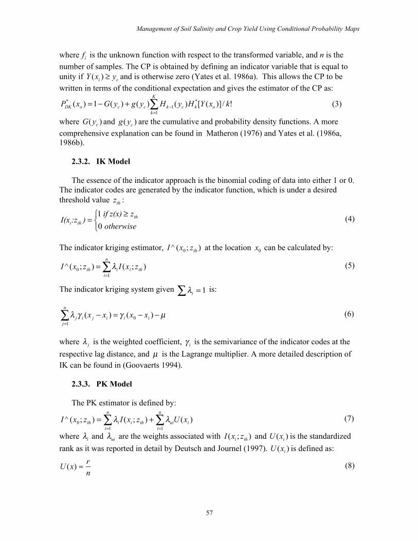
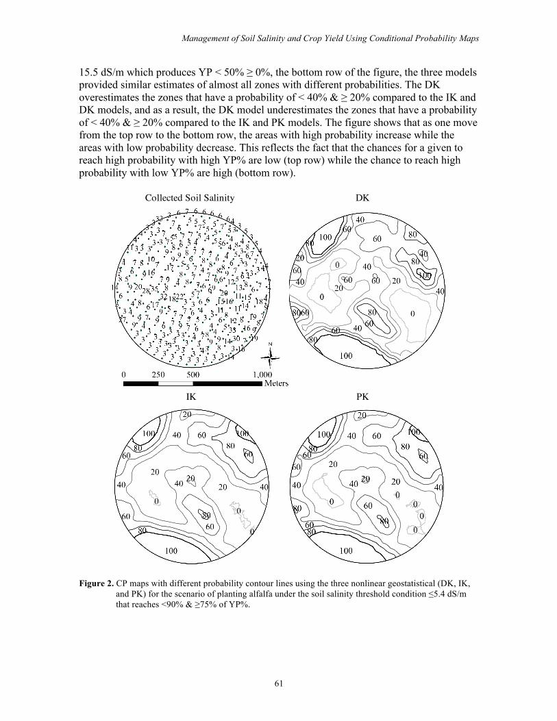
Figure 2 shows the generated CP maps for the scenario of planting a moderately

tolerant crop (alfalfa), under the condition that the soil salinity threshold is ≤5.4 dS/m in order to reach <90% & ≥ 75% of YP%. In addition to the CP maps, the collected soil salinity map - which reveals the spatial distribution of soil salinity points and their values - was also displayed. The field is classified into different zones surrounded by contour lines, and each contour line represents a specific probability in order for this specific zone to reach <90% - 75% of alfalfa YP. The estimation of the three models showed similarities between different zones of different probabilities. For the probability of 100%, the three models were close in estimating the zones in the lower and upper left parts of the field. However, there is a zone in the upper right of the field that both IK and PK models estimated as a 100% probability zone, while the DK model estimated as a 80% probability zone. Of the three models, the DK estimated another zone as a 100% probability zone in the left part of the field inside the < 100 & ≥ 80% probability zone. The zones with a

Eldeiry and Garcia

60

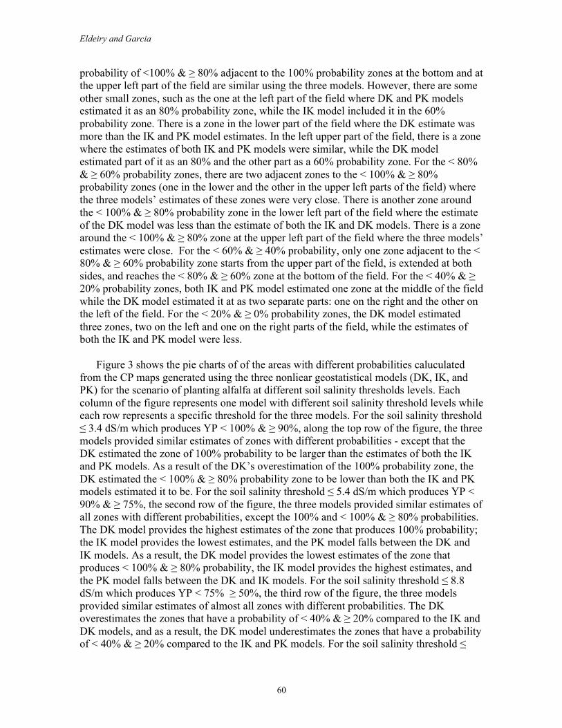
probability of <100% & ≥ 80% adjacent to the 100% probability zones at the bottom and at the upper left part of the field are similar using the three models. However, there are some other small zones, such as the one at the left part of the field where DK and PK models estimated it as an 80% probability zone, while the IK model included it in the 60% probability zone. There is a zone in the lower part of the field where the DK estimate was more than the IK and PK model estimates. In the left upper part of the field, there is a zone where the estimates of both IK and PK models were similar, while the DK model estimated part of it as an 80% and the other part as a 60% probability zone. For the < 80% & ≥ 60% probability zones, there are two adjacent zones to the < 100% & ≥ 80% probability zones (one in the lower and the other in the upper left parts of the field) where the three models’ estimates of these zones were very close. There is another zone around the < 100% & ≥ 80% probability zone in the lower left part of the field where the estimate of the DK model was less than the estimate of both the IK and DK models. There is a zone around the < 100% & ≥ 80% zone at the upper left part of the field where the three models’ estimates were close. For the < 60% & ≥ 40% probability, only one zone adjacent to the < 80% & ≥ 60% probability zone starts from the upper part of the field, is extended at both sides, and reaches the < 80% & ≥ 60% zone at the bottom of the field. For the < 40% & ≥ 20% probability zones, both IK and PK model estimated one zone at the middle of the field while the DK model estimated it at as two separate parts: one on the right and the other on the left of the field. For the < 20% & ≥ 0% probability zones, the DK model estimated three zones, two on the left and one on the right parts of the field, while the estimates of both the IK and PK model were less.

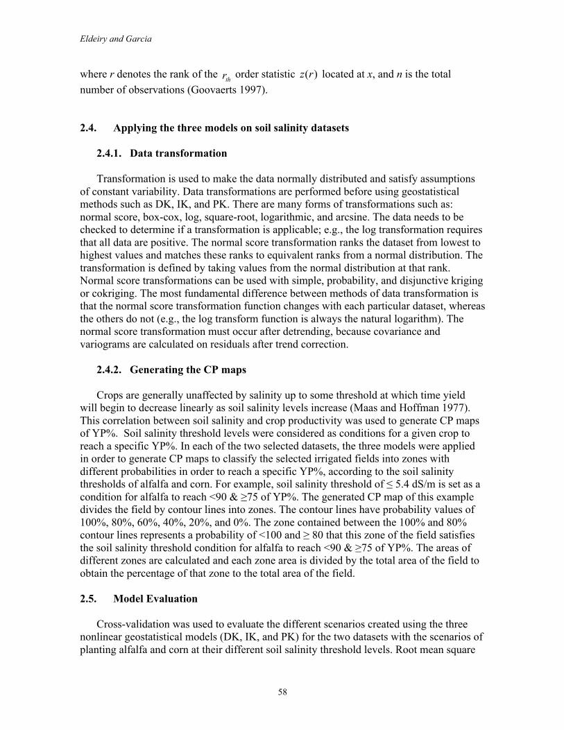
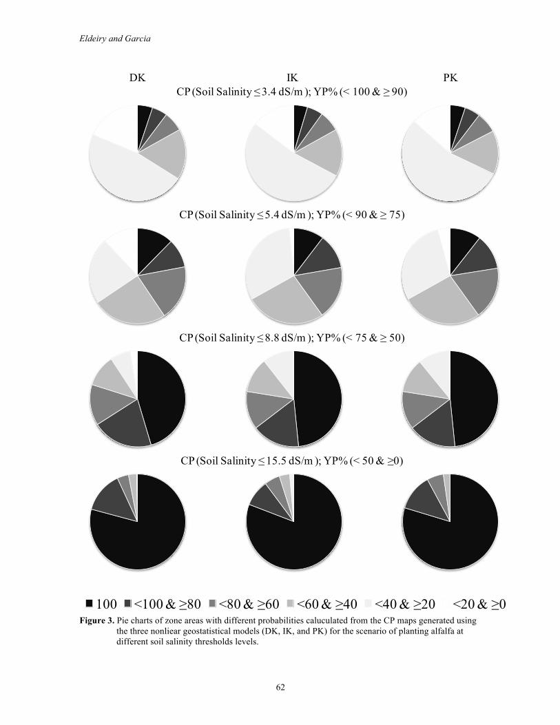
Figure 3 shows the pie charts of of the areas with different probabilities caluculated from the CP maps generated using the three nonliear geostatistical models (DK, IK, and PK) for the scenario of planting alfalfa at different soil salinity thresholds levels. Each column of the figure represents one model with different soil salinity threshold levels while each row represents a specific threshold for the three models. For the soil salinity threshold ≤ 3.4 dS/m which produces YP < 100% & ≥ 90%, along the top row of the figure, the three models provided similar estimates of zones with different probabilities - except that the DK estimated the zone of 100% probability to be larger than the estimates of both the IK and PK models. As a result of the DK’s overestimation of the 100% probability zone, the DK estimated the < 100% & ≥ 80% probability zone to be lower than both the IK and PK models estimated it to be. For the soil salinity threshold ≤ 5.4 dS/m which produces YP < 90% & ≥ 75%, the second row of the figure, the three models provided similar estimates of all zones with different probabilities, except the 100% and < 100% & ≥ 80% probabilities. The DK model provides the highest estimates of the zone that produces 100% probability; the IK model provides the lowest estimates, and the PK model falls between the DK and IK models. As a result, the DK model provides the lowest estimates of the zone that produces < 100% & ≥ 80% probability, the IK model provides the highest estimates, and the PK model falls between the DK and IK models. For the soil salinity threshold ≤ 8.8 dS/m which produces YP < 75% ≥ 50%, the third row of the figure, the three models provided similar estimates of almost all zones with different probabilities. The DK overestimates the zones that have a probability of < 40% & ≥ 20% compared to the IK and DK models, and as a result, the DK model underestimates the zones that have a probability of < 40% & ≥ 20% compared to the IK and PK models. For the soil salinity threshold ≤


61

15.5 dS/m which produces YP < 50% ≥ 0%, the bottom row of the figure, the three models provided similar estimates of almost all zones with different probabilities. The DK overestimates the zones that have a probability of < 40% & ≥ 20% compared to the IK and DK models, and as a result, the DK model underestimates the zones that have a probability of < 40% & ≥ 20% compared to the IK and PK models. The figure shows that as one move from the top row to the bottom row, the areas with high probability increase while the areas with low probability decrease. This reflects the fact that the chances for a given to reach high probability with high YP% are low (top row) while the chance to reach high probability with low YP% are high (bottom row).

Using Conditional Probability Maps to Manage Soil Salinity and Crop Yield

©Hydrology Days

DK

IK PK

Collected Soil Salinity

Figure 3: CP maps for field US14 generated using DK, IK, and PK for sorghum at soil salinity threshold of 5.1 dS/m which produces 90% - 75% of YP. Table 2: The cumulative CP% of the whole field for the three datasets at dif-ferent levels of soil salinity thresholds (different YP%) of alfalfa and corn. YP% DK IK PK Alfalfa Corn Alfalfa Corn Alfalfa Corn

First Dataset 100 100-90 29.5 13.7 29.9 8.2 30.4 90-75 45.7 33.1 47.6 34.8 47.1 34.6 75-50 75.9 52.0 75.9 53.7 75.9 53.9 50-0 93.7 80.9 92.9 81.2 93.9 81.1

Second Dataset 100 100-90 3.2 1.4 90-75 35.7 13.7 36.4 6.0 4.4 1.6 75-50 90.9 44.9 90.4 45.7 10.8 5.5

Figure 2. CP maps with different probability contour lines using the three nonlinear geostatistical (DK, IK,

and PK) for the scenario of planting alfalfa under the soil salinity threshold condition ≤5.4 dS/m that reaches <90% & ≥75% of YP%.

Eldeiry and Garcia

62

DK IK PKCP (Soil Salinity ≤ 3.4 dS/m ); YP% (< 100 & ≥ 90)

CP (Soil Salinity ≤ 5.4 dS/m ); YP% (< 90 & ≥ 75)

CP (Soil Salinity ≤ 8.8 dS/m ); YP% (< 75 & ≥ 50)

CP (Soil Salinity ≤ 15.5 dS/m ); YP% (< 50 & ≥0)

100 <100 & ≥80 <80 & ≥60 <60 & ≥40 <40 & ≥20 <20 & ≥0 Figure 3. Pie charts of zone areas with different probabilities caluculated from the CP maps generated using

the three nonliear geostatistical models (DK, IK, and PK) for the scenario of planting alfalfa at different soil salinity thresholds levels.


63

Table 2. Different zones, as a percentage of the whole field, for the scenarios of planting alfalfa and corn at different soil salinity thresholds and different probabilities for the first dataset.

Soil Salinity Threshold; YP%

Probability 100% <100 & ≥80 <80 & ≥60 <60 & ≥40 <40 & ≥20 <20 & ≥0

Alfalfa, DK ≤ 2.0 dS/m; 100% ≤3.4 dS/m; <100 & ≥90 5.0 5.2 6.6 17.3 47.2 18.7 ≤5.4 dS/m; <90 & ≥75 12.2 9.8 18.7 25.0 22.3 12.0 ≤8.8 dS/m; <75 & ≥50 45.6 20.5 13.7 11.0 6.8 2.5 ≤15.5 dS/m; <50 & ≥0 79.1 13.8 3.9 3.0 0.2 0.0 Alfalfa, IK ≤ 2.0 dS/m; 100% ≤3.4 dS/m; <100 & ≥90 4.6 5.3 7.0 16.0 52.4 14.7 ≤5.4 dS/m; <90 & ≥75 10.2 11.9 18.1 26.8 31.4 1.6 ≤8.8 dS/m; <75 & ≥50 48.5 16.1 12.8 12.0 10.2 0.4 ≤15.5 dS/m; <50 & ≥0 80.9 8.9 5.4 3.3 1.5 0.0

Alfalfa, PK ≤ 2.0 dS/m; 100% ≤3.4 dS/m; <100 & ≥90 5.2 5.2 7.1 14.8 54.2 13.5 ≤5.4 dS/m; <90 & ≥75 10.5 11.9 17.7 26.8 28.9 4.2 ≤8.8 dS/m; <75 & ≥50 48.5 16.1 12.9 11.7 10.5 0.3 ≤15.5 dS/m; <50 & ≥0 79.7 12.5 5.6 2.2 0.0 0.0 Corn DK ≤ 1.7 dS/m; 100% ≤ 2.5 dS/m; <100 & ≥90 0.0 0.1 2.2 7.3 46.7 43.7 ≤3.8 dS/m; <90 & ≥75 7.2 5.2 8.7 20.9 41.0 17.0 ≤5.9 dS/m; <75 & ≥50 14.7 15.8 21.9 20.1 17.9 9.7 ≤10.0 dS/m; <50 & ≥0 54.7 17.7 12.6 9.1 3.8 1.9 Corn IK ≤ 1.7 dS/m; 100% ≤ 2.5 dS/m; <100 & ≥90 0.0 0.0 1.2 6.1 25.1 67.5 ≤3.8 dS/m; <90 & ≥75 7.1 5.5 8.0 19.1 54.2 6.1 ≤5.9 dS/m; <75 & ≥50 11.6 20.9 19.2 24.2 20.9 3.2 ≤10.0 dS/m; <50 & ≥0 56.9 16.3 10.9 8.5 7.0 0.5 Corn PK ≤ 1.7 dS/m; 100% ≤ 2.5 dS/m; <100 & ≥90 0.0 0.0 0.6 4.8 66.6 28.0 ≤3.8 dS/m; <90 & ≥75 7.9 5.7 7.4 18.4 51.7 8.9 ≤5.9 dS/m; <75 & ≥50 12.3 20.3 18.8 24.3 21.6 2.7 ≤10.0 dS/m; <50 & ≥0 56.5 16.5 10.9 8.3 7.7 0.1

Table 2 shows the zones with different probabilities, as a percentage of the whole field, for the scenarios of planting alfalfa and corn at their different soil salinity thresholds for the first dataset. The soil salinity values of the first dataset show that the highest YP% that alfalfa and corn can reach is < 100 & ≥ 90. The table shows that there are similarities and differences ranging from slight to significant in the areas of different zones among the three models. Besides, there are some differences between the scenarios of planting alfalfa and corn in the zones under the same probability and the same YP% for the estimates of the same model when using alfalfa and corn. At the soil salinity threshold ≤ 15.5 dS/m, which causes the alfalfa YP% to be < 50 & ≥ 0 with the probability of < 100 & ≥ 80, the estimations of DK, IK, and PK models were: 13.8, 8.9, and 12.5 respectively. The differences between DK and IK and between IK and PK are significant; however, the

Eldeiry and Garcia

64

difference between DK and PK is slight. At a soil salinity threshold of ≤3.4 dS/m which causes the alfalfa YP% to be < 100 & ≥ 90 with the probability of < 100 & ≥ 80, the estimations of DK, IK, and PK models were: 5.2, 5.3, and 5.2 respectively. This estimation of the different models has only slight differences and sometimes there is no difference at all. Table 2 shows that with the condition that alfalfa and corn reach the same YP%, the areas of different zones of alfalfa are larger than the corresponding ones of corn. At soil salinity thresholds: ≤ 3.4, ≤ 5.4, ≤ 8.8, and ≤ 15.5 dS/m there is a 100% probability for alfalfa YP% to be: < 100 & ≥ 90, < 90 & ≥ 75, < 75 & ≥ 50, and < 50 & ≥ 0 respectively. Table 3. Different zones, as a percentage of the whole field, for the scenarios of planting alfalfa and corn at

different soil salinity thresholds and different probabilities for the second dataset. YP%

Areas within different contour lines 100% <100 & ≥80 <80 & ≥60 <60 & ≥40 <40 & ≥20 <20 & ≥0

Alfalfa, DK ≤ 2.0 dS/m; 100% ≤3.4 dS/m; <100 & ≥90 26.1 13.6 9.9 6.1 20.7 23.7 ≤5.4 dS/m; <90 & ≥75 51.8 6.8 6.9 10.1 14.4 10.0 ≤8.8 dS/m; <75 & ≥50 66.9 10.0 6.9 6.1 6.0 4.1 ≤15.5 dS/m; <50 & ≥0 86.6 3.6 3.6 4.8 1.4 0.0 Alfalfa, IK ≤ 2.0 dS/m; 100% ≤3.4 dS/m; <100 & ≥90 26.7 14.3 7.4 4.6 9.4 37.5 ≤5.4 dS/m; <90 & ≥75 56.3 3.5 3.3 5.0 17.6 14.3 ≤8.8 dS/m; <75 & ≥50 69.0 8.4 7.7 5.2 8.9 0.7 ≤15.5 dS/m; <50 & ≥0 49.4 3.3 3.3 3.3 8.9 31.8 Alfalfa, PK ≤ 2.0 dS/m; 100% ≤3.4 dS/m; <100 & ≥90 27.3 13.5 7.8 4.2 25.6 21.6 ≤5.4 dS/m; <90 & ≥75 57.2 3.2 2.9 3.9 20.8 12.0 ≤8.8 dS/m; <75 & ≥50 68.9 8.4 7.7 5.4 8.2 1.3 ≤15.5 dS/m; <50 & ≥0 84.5 6.1 4.6 3.6 1.2 0.0 Corn DK ≤ 1.7 dS/m; 100% ≤ 2.5 dS/m; <100 & ≥90 ≤3.8 dS/m; <90 & ≥75 40.9 10.9 6.3 8.0 19.3 14.6 ≤5.9 dS/m; <75 & ≥50 57.2 5.3 10.2 8.9 10.8 7.5 ≤10.0 dS/m; <50 & ≥0 71.5 8.6 7.2 3.9 6.0 2.8 Corn IK ≤ 1.7 dS/m; 100% ≤ 2.5 dS/m; <100 & ≥90 ≤3.8 dS/m; <90 & ≥75 49.4 3.3 3.3 3.3 8.9 31.8 ≤5.9 dS/m; <75 & ≥50 57.7 4.2 9.9 9.8 15.0 3.5 ≤10.0 dS/m; <50 & ≥0 70.9 9.7 7.9 5.2 6.3 0.0 Corn PK ≤ 1.7 dS/m; 100% ≤ 2.5 dS/m; <100 & ≥90 ≤3.8 dS/m; <90 & ≥75 49.4 49.4 49.4 49.4 49.4 49.4 ≤5.9 dS/m; <75 & ≥50 58.2 58.2 58.2 58.2 58.2 58.2 ≤10.0 dS/m; <50 & ≥0 70.6 70.6 70.6 70.6 70.6 70.6

The DK model estimation of the corresponding zones was: 5.0, 12.2, 45.6, and 79.1

respectively. At soil salinity thresholds: ≤ 2.5, ≤ 3.8, ≤ 5.9, and ≤ 10 dS/m there is a 100% probability for corn YP% to be < 100 & ≥ 90, < 90 & ≥ 75, < 75 & ≥ 50, and < 50 & ≥ 0


65

respectively. The DK model estimation of the corresponding zones was 0, 7.2, 14.7 and 54.7 respectively. This reflects the fact that alfalfa is a moderate tolerant crop while corn is a moderate sensitive crop. Therefore, the chances for alfalfa are higher than corn to reach high YP%.

Table 3 shows the zones with different probabilities, as a percentage of the whole field, for the scenarios of planting alfalfa and corn at their soil salinity thresholds for the second dataset. The soil salinity values of the second dataset show that the highest YP% that alfalfa can reach is < 100 & ≥ 90 while corn can reach only < 90 & ≥ 75. Table 3 shows that there are fewer similarities among the different models compared to the first dataset, the differences range from slight to significant in the areas of different zones. Also, there are some differences between the scenarios of alfalfa and corn in the zones under the same probability and the same YP% for the estimates of the same model when using alfalfa and corn. At the soil salinity threshold ≤ 3.4 dS/m that alfalfa YP% can reach < 100 & ≥ 90 at the probability of 100%, the estimations of DK, IK, and PK models were 26.1, 26.7, 27.3 respectively, with slight differences. However, at the soil salinity threshold of ≤ 15.5 dS/m that alfalfa YP% can reach < 50 & ≥ 0 at the probability of 100%, the estimations of DK, IK, and PK models were: 86.6, 49.4, and 84.5 respectively. There is a slight difference between the estimates of the DK and PK models, while there is a significant difference between the DK and IK models and between the IK and PK models. At soil salinity thresholds: ≤ 3.4, ≤ 5.4, ≤ 8.8, and ≤ 15.5 dS/m there is a 100% probability for alfalfa YP% to be: < 100 & ≥ 90, < 90 & ≥ 75, < 75 & ≥ 50, and < 50 & ≥ 0 respectively. The DK model estimation of the corresponding zones was: 26.1, 51.8, 66.9, and 86.6 respectively. At soil salinity thresholds: ≤ 2.5, ≤ 3.8, ≤ 5.9, and ≤ 10 dS/m there is a 100% probability for corn YP% to be: < 100 & ≥ 90, < 90 & ≥ 75, < 75 & ≥ 50, and < 50 & ≥ 0 respectively. The DK model estimation of the corresponding zones was 0, 49.9, 57.2 and 71.5 respectively. The differences are significant between the areas of the corresponding zones. The estimates of the DK model range from slight to significant. The DK model estimate of the first zone with alfalfa scenario was 26.1 while its estimate of the similar zone with corn scenario was 0 (significant). In the meanwhile, the model estimates for the second zone with the scario of alfalfa was 51.8 while its estimate for the similar zone with corn was 49.9 (slight).

The previous results show that there are differences from slight to significant among the three models estimates for the different zone. Based on these differences, there is no parameters that tell which model is more accurate than the other. Therefore, cross validation parameters are used to evaluate the estimates of the different models. Table 4 shows the cross validation parameters: MS, RMS, and RMSS for the scenarios of planting alfalfa and corn under the conditions of different soil salinity thresholds using the three models. There are no values for the scenario of planting corn for the three models at YP% of < 100 & ≥ 90 because the soil salinity values are high enough for corn not to reach such YP%. Table 4 shows that the MS values are almost 0’s for all the cases, which means that the estimations of the three models are unbiased. The RMS values are small for all cases, which means that the estimations of the three models are close to the observed values. However, there are some values (0.11, 0.13, and 0.19) of the DK model that are smaller than the IK and PK models. This implies that the DK model is more accurate than the IK

Eldeiry and Garcia

66

and PK models. The RMSS values are close to 1 for most of the cases, which means the three models were accurate in assessing the variability. However, there are a few values of RMSS either greater or less than 1, which means that in these cases the model either overestimates or underestimates the variability. We can consider the RMSS values of 1 as an optimal assessment of the variability, values of RMSS ± 0.05 as a successful estimate of the variability, and values of RMSS out of this range to be less successful in assessing the variability. There are three cases (0.91, 0.91, and 0.93) where the DK model overestimates the variability. There are four cases (0.93, 1.36, 1.16, and 1.39) where the IK model overestimates the variability for the first case and underestimates it with the three other cases. There are four cases (0.91, 1.36, 1.11, and 1.39) where the PK model overestimates the variability for the first case and underestimates it with the three other cases. This gives an indication that the DK model was the most successful in assessing the variability among the three models which confirms the pevious conclusion that the DK is more accurate than the IK and PK models. Table 4. Cross-validation parameters for the scenarios of planting alfalfa and corn under the conditions of

several soil salinity thresholds using the three models. Cross Valid. Coeff.

First Dataset Second Dataset YP%

100 <100&≥90 <90&≥75 <75&≥50 <50&≥0 100 <100&≥90 <90&≥75 <75&≥50 <50&≥0 Alfalfa; DK

MS -0.01 0.00 0.02 0.03 0.01 0.02 0.02 0.01 RMS 0.30 0.38 0.35 0.24 0.11 0.39 0.34 0.11 RMSS 0.91 0.99 0.95 0.91 0.98 0.98 0.96 1.01

Corn; DK MS -0.03 0.01 0.01 0.02 0.01 0.03 0.01 RMS 0.19 0.32 0.39 0.34 0.13 0.43 0.30 RMSS 1.02 0.93 1.01 0.96 0.97 1.00 1.01

Alfalfa; IK MS 0.00 0.00 0.00 0.02 0.01 0.00 0.00 0.01 RMS 0.30 0.39 0.35 0.24 0.09 0.40 0.34 0.11 RMSS 1.00 0.97 0.98 0.93 1.36 0.99 0.97 1.16

Corn; IK MS 0.00 0.00 0.00 0.00 0.01 0.01 0.00 RMS 0.19 0.32 0.41 0.34 0.13 0.44 0.31 RMSS 1.04 0.98 0.98 0.99 1.39 0.99 0.99

Corn; PK MS 0.00 0.00 0.01 0.02 0.02 0.00 0.03 0.01 RMS 0.30 0.38 0.35 0.25 0.09 0.39 0.34 0.11 RMSS 1.01 0.97 0.98 0.91 1.36 0.98 0.98 1.11

Corn; PK MS -0.01 0.00 0.00 0.01 0.01 0.01 0.03 RMS 0.19 0.32 0.40 0.34 0.13 0.43 0.30 RMSS 1.05 1.00 0.99 0.98 1.39 0.98 1.00

The following can help the growers to improve the YP% in the low YP% zone: 1)

improve management of fertilizer application; 2) increase the number of seeds planted; 3) check their irrigation system to make sure that these zones receive the required amount of water; and 4) check for insects in case they need to apply pesticides and herbicides to manage pests


67

4. Conclusion

The techniques presented by the three nonlinear geostatistical models are helpful for managing decision-making for growers who face soil salinity problems. These techniques provide the growers with visual and quantitative information about zones of their fields with different probability to reach a specific YP% for a given crop. These models provide them a quantitative means of evaluating different soil salinity zones in their fields. The information provided in Figures 2 and 3 for the alfalfa and corn scenarios provides the growers with a visual representation of the variation in the probability of YP% in the different zones of their fields when planting either alfalfa or corn. Also, the data presented in Tables 2 and 3 provide the growers with quantitative information about the probability of YP% of different zones in their fields. Based on this information, growers can decide which crop to select. Both visual and quantitative information give the growers warning about the low YP% in their fields. Therefore, growers can pay more attention to these zones, which are mainly affected by soil salinity, to try to alleviate the impact of salinity on these zones and to guarantee that there is no other factor adding another impact beside soil salinity. 5. References Ayers, R.S., Westcot, D.W., 1985. Water quality for agriculture. Food and Agriculture Organization of the

United Nations Rome,, Italy. Burgess, T., Webster, R., 1980a. Optimal Interpolation and Isarithmic Mapping of Soil Properties. II. Block

Kriging. J. Soil Sci. 31, 333–341. Burgess, T.M., Webster, R., 1980b. Optimal Interpolation and Isarithmic Mapping of Soil Properties. Journal

of Soil Science 31, 333–341. Cain, D., 1997. U.S. Geological Survey Date Collection Center and Studies in the Arkansas River Basin. Carr, J.R., Myers, D.E., 1990. Efficiency of different equation solvers in cokriging. Computers &

Geosciences 16, 705–716. Carr, J.R., Myers, D.E., Glass, C.E., 1985. Cokriging—a computer program. Computers & Geosciences 11,

111–127. Cressie, N., 1992. Statistics for Spatial Data. Terra Nova 4, 613–617. Deutsch, C., 1989. DECLUS: a FORTRAN 77 program for determining optimum spatial declustering

weights. Computers & Geosciences 15, 325–332. Deutsch, C.V., Journel, A.G., 1997. GSLIB: Geostatistical Software Library and User’s Guide, 2nd ed.

Oxford University Press, USA. Eldeiry, A., Garcia, L., 2008a. Spatial Modeling of Soil Salinity Using Remote Sensing, GIS, and Field Data.

VDM Verlag. Eldeiry, A.A., Garcia, L.A., 2008b. Detecting Soil Salinity in Alfalfa Fields using Spatial Modeling and

Remote Sensing. Soil Science Society of America Journal 72, 201. Eldeiry, A.A., Garcia, L.A., 2010. Comparison of Ordinary Kriging, Regression Kriging, and Cokriging

Techniques to Estimate Soil Salinity Using LANDSAT Images. Journal of Irrigation and Drainage Engineering 136, 355.

Eldeiry, A.A., Garcia, L.A., 2011. Using Indicator Kriging Technique for Soil Salinity and Yield Management. Journal of Irrigation and Drainage Engineering 137, 82–93.

Eldeiry, A.A., Garcia, L.A., Reich, R.M., 2008. Soil Salinity Sampling Strategy Using Spatial Modeling Techniques, Remote Sensing, and Field Data. Journal of Irrigation and Drainage Engineering 134, 768–777.

Eldeiry and Garcia - 2008 - Detecting Soil Salinity in Alfalfa Fields using Sp.html, n.d. . Eldeiry and Garcia - 2010 - Comparison of Ordinary Kriging, Regression Kriging.html, n.d. . Frasier, W.M., 1999. Irrigation management in Colorado: survey data and findings.

Eldeiry and Garcia

68

Gates, T.K., Burkhalter, J.P., Labadie, J.W., Valliant, J.C., Broner, I., 2002. Monitoring and Modeling Flow and Salt Transport in a Salinity-Threatened Irrigated Valley. Journal of Irrigation and Drainage Engineering 128, 87–99.

Ghassemi, F., Jakeman, A.J., Nix, H.A., 1995. Salinisation of land and water resources: human causes, extent, management and case studies. CAB international.

Goovaerts, P., 1994. Comparative performance of indicator algorithms for modeling conditional probability distribution functions. Mathematical geology 26, 389–411.

Goovaerts, P., 1997. Geostatistics for natural resources evaluation. Oxford University Press. Halvorson, J.J., Smith, J.L., Bolton, H.J., Rossi, R.E., 1995. Evaluating shrub-associated spatial patterns of

soil properties in a shrub-steppe ecosystem using multiple-variable geostatistics. Soil Science Society of America Journal 59, 1476–1487.

Hillel, D., 2000. Salinity management for sustainable irrigation: integrating science, environment, and economics. World Bank Publications.

Isaaks, E.H., 1984. Risk qualified mappings for hazardous waste sites: a case study in distribution free geostatistics. Stanford University.

Jones, R., Marshall, G., 1992. Land salinisation, waterlogging and the agricultural benefits of a surface drainage scheme in Benerembah irrigation district. Review of Marketing and Agricultural Economics 60.

Journel, A.G., 1983. Nonparametric estimation of spatial distributions. Journal of the International Association for Mathematical Geology 15, 445–468.

Journel, A.G., 1989. Fundamentals of geostatistics in five lessons. American Geophysical Union. Juang, K.-W., Lee, D.-Y., 1998. Simple Indicator Kriging for Estimating the Probability of Incorrectly

Delineating Hazardous Areas in a Contaminated Site. Environ. Sci. Technol. 32, 2487–2493. Lyon, S.W., Lembo Jr., A.J., Walter, M.T., Steenhuis, T.S., 2006. Defining probability of saturation with

indicator kriging on hard and soft data. Advances in Water Resources 29, 181–193. Maas, E., Hoffman, G., 1977. Crop Salt Tolerance$\backslash$-Current Assessment. Journal of the Irrigation

and Drainage Division 103, 115–134. Matheron, G., 1976. A Simple Substitute for Conditional Expectation Kriging., in: Advanced Geostatistics in

the Mining Industry: Proceedings of the NATO Advanced Study Institute Held at the Istituto Di Geologia Applicata of the University of Rome, Italy, 13-25 October 1975. p. 221.

Van Meirvenne, M., Goovaerts, P., 2001. Evaluating the probability of exceeding a site-specific soil cadmium contamination threshold. Geoderma 102, 75–100.

Miles, D.L., 1977. Salinity in the Arkansas valley of Colorado. Region VIII, Environmental Protection Agency.

Myers, D.E., 1982. Matrix formulation of co-kriging. Mathematical Geology 14, 249–257. Oyedele, D., Amusan, A., Olu Obi, A., 1996. The use of Multiple-Variable Indicator Kriging technique for

the assessment of the suitability of an acid soil for maize. Tropical agriculture 73, 259–263. Richmond, A., 2002. An alternative implementation of indicator kriging. Computers & geosciences 28, 555–

565. Russo, D., 1984a. A Geostatistical Approach to the Trickle Irrigation Design in a Heterogeneous Soil 2. A

Field Test. Water Resources Research 20, 543–552. Russo, D., 1984b. Design of an Optimal Sampling Network for Estimating the Variogram. Soil Science

Society of America Journal 48, 708–716. Schepers, J., Schlemmer, M., Ferguson, R., 2000. Site-specific considerations for managing phosphorus. Smith, J.L., Halvorson, J.J., Papendick, R.I., others, 1993. Using multiple-variable indicator kriging for

evaluating soil quality. Soil Sci. Soc. Am. J 57, 743–749. Solow, A.R., 1986. Mapping by simple indicator kriging. Mathematical geology 18, 335–352. von Steiger, B., Webster, R., Schulin, R., Lehmann, R., 1996. Mapping heavy metals in polluted soil by

disjunctive kriging. Environmental Pollution 94, 205–215. Sullivan, J., 1984. Conditional recovery estimation through probability kriging–theory and practice.

Geostatistics for natural resources characterization. Reidel, Dordrecht 365–384. Tanji, K.K., 1990. Agricultural salinity assessment and management. Amer Society of Civil Engineers. Triantafilis, J., Odeh, I.O.A., Jarman, A.L., Short, M.G., Kokkoris, E., 2004. Estimating and mapping deep

drainage risk at the district level in the lower Gwydir and Macquarie valleys, Australia. Aust. J. Exp. Agric. 44, 893–912.


69

Triantafilis, J., Odeh, I.O.A., McBratney, A.B., 2001. Five geostatistical models to predict soil salinity from electromagnetic induction data across irrigated cotton. Soil Science Society of America Journal 65, 869–878.

Webster, R., Burgess, T.M., 1980. Optimal Interpolation and Isarithmic Mapping of Soil Properties. III Changing Drift and Universal Kriging. Journal of Soil Science 31, 505–524.

Webster, R., Oliver, M.A., 1989. Optimal interpolation and isarithmic mapping of soil properties. VI. Disjunctive kriging and mapping the conditional porbability. Journal of Soil Science 40, 497–512.

Wittler, J.M., Cardon, G.E., Gates, T.K., Cooper, C.A., Sutherland, P.L., 2006. Calibration of Electromagnetic Induction for Regional Assessment of Soil Water Salinity in an Irrigated Valley. Journal of Irrigation and Drainage Engineering 132, 436–444.

Wood, G., Oliver, M.A., Webster, R., 1990. Estimating soil salinity by disjunctive kriging. Soil Use and Management 6, 97–104.

Yates, S., Warrick, A., Matthias, A., Musil, S., 1988. Spatial variability of remotely sensed surface temperatures at field scale. Soil Sci. Soc. Am. J 52, 40–45.

Yates, S.R., Warrick, A.W., Myers, D.E., 1986a. Disjunctive Kriging: 2. Examples. Water Resour. Res. 22, PP. 623–630.

Yates, S.R., Warrick, A.W., Myers, D.E., 1986b. Disjunctive Kriging: 1. Overview of Estimation and Conditional Probability. Water Resour. Res. 22, PP. 615–621.

Zirschky, J., 1985. Geostatistics for environmental monitoring and survey design. Environment international 11, 515–524.

Zirschky, J., Keary, G.P., Gilbert, R.O., Middlebrooks, E.J., 1985. Spatial Estimation of Hazardous Waste Site Data. Journal of Environmental Engineering 111, 777–789.

Zirschky, J.H., Harris, D.J., 1986. Geostatistical Analysis of Hazardous Waste Site Data. Journal of Environmental Engineering 112, 770–784.

management of soil salinity and crop yield using...

Documents