critical path analysis using simulation techniques and selection
TRANSCRIPT

i
CRITICAL PATH ANALYSIS USING SIMULATION TECHNIQUES AND
SELECTION OF LEAN TOOLS TO MULTIPLE CRITICAL PATHS BASED ON COST
FACTOR
A Thesis by
Mervyn John
Bachelor of Engineering, PSG College of Technology, India, 2009
Submitted to the Department of Industrial and Manufacturing Engineering and the faculty of the Graduate School of
Wichita State University in partial fulfillment of
the requirements for the degree of Master of Science
December 2011

i
© Copyright 2011 by Mervyn John
All Rights Reserved

iii
CRITICAL PATH ANALYSIS USING SIMULATION TECHNIQUES AND
SELECTION OF LEAN TOOLS TO MULTIPLE CRITICAL PATHS BASED ON COST
FACTOR
The following faculty members have examined the final copy of this thesis for form and content, and recommend that it be accepted in partial fulfillment of the requirement for the degree of Master of Science with a major in Industrial Engineering.
___________________________________
Krishna K. Krishnan, Committee Chair
___________________________________
Mehmet B. Yildirim, Committee Member
___________________________________
Ramazan Asmatulu, Committee Member

iv
ACKNOWLEDGMENTS
It is a great pleasure to thank all the people who made this thesis possible.
I owe my deepest gratitude to my advisor Dr. Krishna K. Krishnan who helped me in all
my problems regarding my research.
I would like to thank my committee members Dr. Bayram Yildirim and Dr. Ramazan
Asmatulu who took time to review my thesis and gave some valuable suggestions and help hone
my research
I also thank the members of Facilities Planning and Logistics Research Group who
helped me in the completion of my thesis.
I would like to specially thank Prakash, Sathya, Suresh,
Mukund,Prasanna,Thiagaraj,Shokufeh, Kaushik, Varun, Thejas, Sailesh and Hanger for their
valuable time to discuss and give suggestions invaluable to my research and constant support
during my time of need.
Finally, I would like to dedicate this thesis to my familywho are the most precious people
in my life.

v
ABSTRACT
A production system converts raw materials into finished goods by various processes.
The processes could occur parallel in order to reduce the time taken to complete the processes.
Critical path in production systems is the maximum time taken to complete processes occurring
in parallel. Identifying critical paths are important because, in order to improve the cycle time
emphasis needs to be given to the critical path. Critical path is usually a single path in
deterministic processing times. Due to variability more than one path might tend to be critical
within the same system. The initial part of this research focuses on identifying changes in critical
paths in variable processing times and prioritization of paths. Several metrics such as critical
path severity index, all path severity indexes, probability of critical path beyond standard time
are used to identify the criticality of paths. Next, suitable tools are implemented within these
paths in order to improve the probability of completion and reduce the costs due to delay. An
economic analysis for using lean tools within the paths is done. The allocation of improvement
tools is based on the variability of each process and the processing time

vi
TABLE OF CONTENTS
Chapter Page
1INTRODUCTION .........................................................................................................................1
1.1 Problem Background ...............................................................................................1
1.2 Production System ...................................................................................................2
1.3 Critical Path .............................................................................................................2
1.4 Critical path in workstations ....................................................................................3
1.5 Variable processing times ........................................................................................3
1.6 Lean Manufacturing .................................................................................................4
1.7 Research purpose .....................................................................................................4
1.8 Research objectives ..................................................................................................5
2LITERATURE REVIEW ..............................................................................................................6
2.1 Introduction ..............................................................................................................6
2.2 Production Systems ..................................................................................................6
2.3 Variability in production systems ............................................................................7
2.4 Network programming .............................................................................................8
2.5 Critical path ............................................................................................................10
2.6 Fuzzy Critical path .................................................................................................12
2.7 Project Evaluation and Review Technique (PERT)...............................................12
2.8 Lean implementation .............................................................................................13
2.9 Research motivation...............................................................................................14
3CRITICAL PATH IDENTIFICATION METHODOLOGY.......................................................15
3.1 Introduction ............................................................................................................15

vii
TABLE OF CONTENTS (continued)
Chapter Page
3.2 Notations ................................................................................................................16
3.3 Assumptions ...........................................................................................................17
3.4 Critical path identification .....................................................................................18
3.4.1 Deterministic processing time....................................................................18
3.4.2 Stochastic processing time .........................................................................19
3.4.3 Identification of critical path ......................................................................20
3.4.3.1 Mathematical Formulation .............................................................20
3.4.3.2 Algorithm .......................................................................................21
3.4.3.3 Flowchart .......................................................................................23
3.4.4 Move rate ...................................................................................................24
3.4.4.1 Mathematical Formulation .............................................................26
3.4.4.2 Algorithm .......................................................................................25
3.4.4.3 Flowchart .......................................................................................26
3.4.5 Critical Path Severity Index (CSI) .............................................................27
3.4.5.1 Algorithm .......................................................................................28
3.4.5.2 Flowchart .......................................................................................29
3.4.6 Severity Index for paths (β) ......................................................................29
3.4.6.1 Algorithm .......................................................................................30
3.4.6.2 Flowchart .......................................................................................31
3.5 Case Study – 3 workstations- 27 processes ...........................................................32
3.5.1 Deterministic Case .....................................................................................34

viii
TABLE OF CONTENTS (continued)
Chapter Page
3.5.2 Stochastic Case ..........................................................................................34
3.5.2.1 Critical path due to variability .......................................................36
3.5.2.2 Critical path shift based on standard time ......................................36
3.5.2.3 Frequency beyond standard time ...................................................37
3.5.2.4 Critical path severity index (CSI) ..................................................39
3.5.2.5 Severity index for all paths ............................................................40
3.6 Conclusion .............................................................................................................42
4LEAN IMPLEMENTATION ......................................................................................................43
4.1 Introduction ............................................................................................................43
4.2 Assumptions ...........................................................................................................43
4.3 Model input requirements ......................................................................................44
4.4 Mathematical Model ..............................................................................................44
4.5 Case Study: High variability 3 workstations – 9 paths and 27 processes ..............45
5STUDY OF CRITICAL PATH BASED ON VARIABILITY....................................................50
5.1 Variability Levels...................................................................................................50
5.2 No variability .........................................................................................................52
5.3 Low variability case ...............................................................................................54
5.4 Medium variability case .........................................................................................56
6CONCLUSION AND FUTURE RESEARCH ............................................................................61
6.1 Conclusion .............................................................................................................61
6.2 Future research .......................................................................................................62

ix
TABLE OF CONTENTS (continued)
Chapter Page
REFERENCES ..............................................................................................................................63

x
LIST OF TABLES
Table Page
2.1 Recommended scheduling tool for different industries (Yamin & Harmelink, 2001)9
2.2 Disadvantages of PERT (Schoderbek, 1965) 13
3.1 Types of variability (Hopp, & Spearman, 2001) 20
3.2 Variability based on CSI 28
3.3(a) Processing times for workstation 1 34
3.3(b) Processing times for workstation 2 34
3.3(c) Processing times for workstation 3 34
3.4 Critical path for workstation 1 36
3.5 Frequency of a critical path exceeding the standard cycle time 38
3.6 Critical path severity index for workstation 1 40
3.7 All path severity index for workstation 1 42
3.8 Comparison of the Metrics 43
4.1 Cost of Lean Experiment and improvement 47
4.2 Identification of the worst process 48
4.3 Improvement for path b in workstation 3 49
4.4 Improvement based on criticality 50
4.5 Lean implementation based on payback period 51
5.1 Critical path analysis for deterministic case 54
5.2 Order of Lean Experiments in Deterministic case 55
5.3 Critical path analysis for low variability case 56

xi
LIST OF TABLES (continued)
Table Page
5.4 Order of Lean Experiments in less variability scenario 57
5.5 Critical path analysis for medium variability case 58
5.6 Order of Lean Experiments in medium variability scenario 59
5.7 Order of lean experiments based on probability of completion 60
5.8 Order of lean experiments based on payback period 61

xii
LIST OF FIGURES
Figure Page
1.1 Representation used for critical path method 3
3.1 Process configurations within a workstation 19
3.2 Line diagram for the production system 33
3.3 Line diagram of workstation 1 33
3.4 Probability of path being critical for all the workstations 37
3.5 Probability of a critical path exceeding the standard time 39
3.6 Critical path severity indexes for all the workstations 41
3.7 All path severity indexes for all the workstations 42
4.1 Probability of completion for all workstations 48
5.1 Distributions for process 1 in line 1 for workstation 1 53
.

1
CHAPTER 1
INTRODUCTION
1.1 Problem background
A facility is an integral component in a business enterprise. An efficient facility provides
an edge over competitors such asfaster delivery of parts without delay and with lower
fluctuations in the processing time between workstations. Production systems convert raw
materials into finished goods that provide value to the customer. Production systems consist of
workstations either in parallel, series or a combination of series and parallel. In order to improve
an existing complex production system, which involves many operations occurring in series and
parallel, the dominating path needs to be analyzed. The path that takes the maximum time to
complete the process is defined as the critical path for that process. But in production systems
with high variability and low volume such as ship building industries and aircraft manufacturing
industries, the processing times have a high variability as most operations are labor intensive.
Various other factors such as part outages and tool unavailabilityalso contribute to variability. In
order to decrease processing time and variability, improvement needs to be done in the critical
path. Else any improvements made on other non-critical paths would not help in decreasing the
cycle time for the workstation. When the processing times are deterministic, it is easy to see that
only one of the lines could be a critical path. But, in industries such as aircraft manufacturing,
there is a trend of high variability in the processing times due to manual labor and process
variation. Due to the high variability, more than one critical path could dominate the system. So,
if emphasis is given only to one critical path, there might not be any significant difference in the
time taken to complete a part. In such a scenario, more than one path needs to be analyzed
simultaneously in order to reduce the time taken to complete a part. Thus, a study has been done

2
to identify the possibilities of more than one path being critical and the significance of each of
the contributing factors.
1.2 Production System
A production system involves a set of processes that convert raw materials into finished
goods which is valued in the eyes of the customer. The set of processes involved can either be in
series, parallel, or a combination of both. One of the problems faced in production systems is the
completion of processes within a fixed standard time. The delays could be due to variability,
shortage of resources, machine breakdowns, high travelling time between workstations,
bottleneck machine and tool failure. In order to satisfy the customer, parts have to be supplied at
the right cost, in the right quantity and at the right time. Delays in the production line could result
in penalties in the form of lost orders and high work in process inventory cost.
1.3 Critical Path
Critical path is the maximum time taken to complete the process when there are no
external delays that are not accounted for. It is used to calculate the time taken to complete a set
of operations when the processing times are certain. Non-critical path(s) completes the
operations within the time taken at the critical path. To calculate time taken at each path, the
critical path is represented as an activity and each process is represented by a node as shown in
Figure 1.1.

3
Figure 1.1 Representation used for critical path method
1.4 Critical path in workstations
Critical path in a production system is the path that takes the maximum time to complete
all the processes. Time taken at the critical path within a workstation of parallel and serial
processes determines the cycle time for that workstation. Thus, in order to reduce the time taken
at the workstation, critical path needs to be analyzed at first. In production systems, data is
stochastic and variability leads to more than one part being critical at the same time.
1.5 Variable processing times
Many techniques have been used to calculate the time of completion within a machine.
Research has been done to calculate the time of completion when the processing time is
deterministic and the activities are independent by using Critical Path Method (CPM). Program
Evaluation and Review Technique (PERT) analysis is used to calculate the time of completion
when the processing time is uncertain assuming that the critical path calculated by the critical
path method is the same. However, previous research does not consider the shifts in critical path
when there are stochastic processing times. Variable processing times occur mostly in
manufacturing systems which have manual labor. Suer (1996) classified manufacturing systems

4
as either labor intensive or machine intensive. Variability is dominant in labor intensive
manufacturing system because of manual labor such as tool change, loading and unloading
material from the machine transferring parts.
1.6 Lean Manufacturing
Lean manufacturing is a philosophy implemented by Toyota Production System (TPS) in
Japan. Lean manufacturing aims to identify all the activities and resources within a firm or
industry as value added activities, non- value added activities and necessary non-value added
activities. This philosophy identifies value added activity as any process or resource, that adds
value to the product and non-value added activity as the process that do not add any value to the
product and needs to be eliminated. Necessary non-value added activities are the activities that
do not add value to the product, but are necessary and cannot be eliminated due to external
factors like variability though they can be reduced. Various tools are used to improve the
efficiency of the system, tools can be used to either reduce the processing time or reduce the
variability in the system.
1.7 Research purpose
In workstations which have several thousands of tasks mostly distributed in series and
parallel, the cycle time of a workstation is defined by the time taken at the critical path. Due to
variability, there are instances when more than one path tends to be critical within the same
workstation, which could cause the time taken at the workstation to exceed the standard cycle
time. In these cases, in order to reduce the cycle time, emphasis needs to be given to more than
one workstation. This research studies how much influence does each path in the system has in
the probability of completion and ensure that the parts are produced within the standard cycle

5
time. A study on the shift in critical path is also done along with the probability of each part
being critical.
1.8 Research objectives
The objectives of this research:
1. Identification of critical path(s) in stochastic processing times
2. Calculation of probability of a part being critical:
a. Without consideration to standard time
b. Considering the standard time
3. Calculation of the average time a path exceeds from the standard move rate
4. Improving the probability of completion
5. Implementing lean techniques within the system so as to reduce the costs due to delay
The research work has been organized into five chapters. Chapter 2 provides the existing
literature and methodologies used to identify critical path(s) and lean tools used to reduce costs.
Most of the literature is for deterministic values and chapter 3 provides a detailed methodology
on the identification of critical paths and prioritizing them for improvement and chapter 4
includes application of lean tools to the critical paths and improving the probability of
completion, thus, improving the existing system with the minimal cost and available resources.
Chapter 5 is the conclusion of calculation of critical paths and application of lean techniques in
order to improve the performance of the system. It also includes future research in the field of
critical path in variable processing times.

6
CHAPTER 2
LITERATURE REVIEW
2.1 Introduction
The purpose of this research is to analyze a given production system, which involves
several operations in series and parallel. The research done in production systems is based on
low volume and high variability, such as, aircraft manufacturing industries and ship building.
Section 2.2 discusses production systems followed by section 2.3 which involves a study on the
effects of variability in a production system. Section 2.4 focuses on network programming
models used to calculate the time taken to complete a set of processes within a network based on
complexity of the model used. Section 2.5 discusses the methods used to identify the critical path
and calculate the time taken at the critical path which in turn is used to calculate the time taken to
complete the set of operations. The next section is about using fuzzy numbers used to calculate
critical paths. Section 2.7 deals with calculating the time taken to complete a set of operations
using Project Evaluation Review Technique (PERT) and the drawbacks of using PERT analysis.
Section 2.8 includes implementing lean techniques in critical path analysis to reduce the
processing time based on economic analysis which is followed by the research motivation in
section 2.9.
2.2 Production Systems
Production line is a system that converts the given raw material to the finished goods
based on the customer’s requirement by using the minimal tools in a highly efficient manner.
Certain processes could take higher processing times than other processes. This is due to
difference in time taken to complete the process, tool unavailability, waiting time and machine
downtime. According to Suer (1996), production systems are classified into machine intensive
7
and labor intensive production system. In order to do accurate operations such as gripping,
manual labor is required (Bi and Zhang, 2001).
Production systems such as aircraft manufacturing industries involve low volume and
highly customized goods that are nearly all the aircrafts built are based on the customer’s
requirements. In such systems, there exists high variability in many processes within the line.
2.3 Variability in production systems
Production system converts raw material into finished goods which are valued in the eyes
of the customer through a series of operations or processes. Production systems can be classified
into machine intensive production system and labor intensive production system (Suer, 1996). In
a machine intensive production system, the factors that decide the productivity of the system is
primarily based on the number of machines available in the production system and does not
depend on the labor present in the system. In labor intensive production systems, the factors that
influence the productivity are the labor present in the system. The workers are allotted with
inexpensive equipment to perform the operations (Pachaimuthu, 2010). In labor intensive
manufacturing systems, due to the high involvement of labor, the variability tends to be more
due to worker absenteeism, skill level required to perform the task, change in worker
productivity within the day and breaks.
Production lines were initially developed based on high volume and for standardized
products. So emphasis was given to highest utilization and high labor specialization (Shtub and
Dar-El, 1989 & Scholl, 1999). Due to product standardization, the lines could be balanced
perfectly. But due to an increase in demand and global competition, the demand for customized
goods and services were expected. Due to an increase in product volume within the line, the
variations also increased.

8
2.4 Network Programming
Various network programming techniques are used to evaluate the time taken to complete
products and meet the deadlines of various lines. The various network programming techniques
are Critical Path Method (CPM), Project Evaluation and Review Technique (PERT), Bar/Gantt
chart, Line of Balance (LOB), Vertical Production Method (VPM), and Linear Scheduling
Model (LSM).
Gantt chart is a tool used to schedule based on the start and finish time. The advantages
of using are that Gantt charts are simple to use, they take less time to create. The disadvantage of
using Gantt charts is that it becomes tough to implement in complex production systems having
variable processing time. They also fail to show the dependencies of various processes. Gantt
chart works better in simple production systems. When the complexity of a production system
increases, or if the production systems has variable processing time, Gantt charts cannot be used
to schedule start and finish time.
Line of Balance (LOB) is used in areas where repetition of jobs occurs. Linear
Scheduling Method (LSM) is used to represent the location and time operations when they occur.
The above networking models are not feasible for complex production systems.
Based on the type of industry and the work required, various models have proven to be
efficient (Yamin & Harmelink, 2001). Table 2.1 shows which scheduling method is optimal for
which type of industry based on complexity of production system and the number of activities
required completing.

9
Table 2.1 Recommended scheduling tool for different industries (Yamin &
Harmelink, 2001)
Type of
industry Application Scheduling
Method Main Characteristic
Linear and continuous
projects
Pipelines, railroads, tunnels and highways
LSM • Few activities • Executed along a linear path/
space • Hard sequence logic • Work continuity crucial for
effective performance
Multi-unit repetitive projects
housing complex, buildings
LOB • Final product a group of similar units
• Same activities during all projects
• Balance between different activities achieved to reach objective production
High-rise buildings
LOB, VPM • Repetitive activities • Hard logic for some activities,
soft for others • Large number of activities • Every floor considered a
production unit
Very complex processes
Refineries, aircraft manufacturing
PERT/CPM • Extremely large number of activities
• Complex design • Activities discrete in nature • Crucial to keep project in critical
path
Simple projects any kind Bar/Gantt chart
• Indicates only time dimension (when to start and end activities)
• Relatively few activities
From the table, it can be inferred that for an aircraft industry which involves a lot of
complex operations, the most optimal networking techniques include are Project Evaluation
Review Technique (PERT) and Critical Path Method (CPM). CPM method uses deterministic
values to calculate the time for completion for various operations PERT method overcomes the
deterministic concept of processing time by using a beta distribution. PERT method calculates
the completion time by considering the highest time to complete the task, least time to complete

10
the task and the most common time to calculate the critical path. PERT cannot be used if the data
follows a distribution other than beta distribution (Chanas & Zielinski, 2001).
2.5 Critical Path
Critical Path Method (CPM) technique was developed by E.I. DuPont de Nemours and
company in conjunction with the Univac Applications Research Center of Remington Rand
(Wickwire and Smith, 1975). It has gained popularity ever since and is used to calculate the time
taken to complete a project.
Critical path is the maximum time taken to complete a set of processes when parallel
operations occur. Generally, the path that takes the maximum time to complete the given set of
operations determines the rate at which a process comes out. This path is called the critical path.
In deterministic data, the critical path can be calculated by simply calculating the sum of the
times taken by individual processes within the workstation. In stochastic data, the critical path is
calculated the same way by adding the individual processing times. But, due to variability more
than one path could tend to dominate the system.
According to Winston (1994) various rules need to be considered when coining analysis
using critical path method. The various rules used for critical path analysis are shown below.
Rule 1. Activities for parallel processing must start at a node.
Rule 2. The activities must end at the completing node.
Rule 3. The number of nodes need to be numbered such that the completion node has a
larger number than the starting node.
Rule 4. An activity should not be represented with more than one node.
Rule 5. If two nodes need to be connected with more than one arc then a dummy arc is
used to trigger the activity.
11
Previous researches by Nasution (1994) analyzed critical path with the earliest time a part
comes out and the latest time a path comes out based on interactive fuzzy logic techniques.
Mount Clemens General Hospital (MCGH) used critical path method to improve the total
quality management in clinical areas (Hofmann P.A., 1991). The warm up time considered was
around 44 patients and critical path analysis was considered after the warm up period. A
complication rate of around 5% was in the critical path when compared to a 16% rate for no
guided care. After the identification of the critical path, a steering committee was formed
comprising of members from hospital administration, nursing, quality assurance and risk
management for further investigation. It was found that critical path method was a very effective
tool for an environment of communication and commitment.
2.6 Fuzzy critical path method
According to Chanas and Zielinski (2001), critical paths assume the task time to be
deterministic, but in real scenarios those are usually not true. They analyzed the criticality of
each path for various cases using fuzzy logic. In the late 1900s, researches (J.J.Buckley, 1989;
S.Chanas, 1982; S.Chanas and J. Kamburowski, 1981; S.Chanas and E. Radosinski, 1976; I.S.
Chang, Y. Tsujimura, M. Gen, T. Tozawa,1995, H. Prade, 1979; H. Rommelfanger, 1994; A.I.
Slyeptsov, T.A. Tyshchuk, 1997; A.I. Slyeptsov, T.A. Tyshchuk, 1999, J.S. Yao, F.T. Lin, 2000)
on critical path analysis was done using fuzzy logic in critical path method wherein fuzzy
numbers were used to model activity times. Common deterministic numbers were replaced by
fuzzy numbers which in turn had modified dependencies. The project characteristics were
defined based on these properties.

12
2.7 Project Evaluation and Review Technique (PERT)
PERT overcomes the deterministic task time by assuming random variables following
beta distributions to model the activity times (Malcolm, Roseboom, Clark& Fazar, 1959). Many
papers have been published regarding PERT analysis ever since, but all the papers focused on the
path task times following a beta distribution. PERT analysis is based on the determining activity
times based on optimistic ‘a’, most likely ‘m’ and pessimistic ‘b’ activity times (Ginzbufg,
1988).
Ginzbufg (1988) concludes that the‘most likely activity time’ is useless. PERT analysis is
highly complex for large networks (Schoderbek, 1965). A survey was conducted based on 81
respondents which is shown in table 2.2
Table 2.2 Disadvantages of PERT (Schoderbek, 1965)
Disadvantages Number % Respondents
Excess of work 16 19.7
Training of personnel in PERT 9 11.1
Inflexibility of the system 54 66.6
Cost of application 19 23.5
Too much reliance on PERT 21 25.9
None 4 4.9
Other 20 24.7
Don’t know 1 1.2
Not Ascertained 4 4.9

13
Research has not been done to calculate the change in a critical path and the probability
of other paths being critical using simulation as a tool. This research aims to focus on a high
variable system and identify the probability of each path being critical.
2.8 Lean Implementation
According to Achanga, Shebah, Roy and Nelder (2006), productivity improvement
techniques such as lean manufacturing can be used to improve the existing process. Successful
implementation of lean can be achieved by enhanced critical decision processes. Their research
suggests that proper funds need to be allocated to improvement processes or else no significant
improvement can be seen within the company. Workforce training is also crucial to lean
implementation.
Research was done in an aircraft manufacturing industry to improve the probability of
completion within various workstations, so that parts complete the operations within the standard
move rate. Standard move rate is the time within which the operations need to be completed. If
the operations do not complete within the standard move rate, parts move to the next workstation
and previous operations also take place at the next workstation. Various lean tools were used to
improve the existing process in an aircraft manufacturing system. The lean metric used for the
analysis was probability of completion (PC). Probability of completion is the probability that the
processes complete within the standard time. Based on their research, the probability of
completion was low, so lean tools were used to improve the probability of completion. Various
strategies were used to improve the probability of completion (PC) to 75%, 80% and 85% all the
time (Durgaparameswaran, 2010). The costs for implementation significantly increased when the
probability of completion increased. Lean tools were used to improve the probability of
completion of a set of tasks in an aircraft industry. Various combinations of options were

14
suggested based on the cost of implementing the tools and on the improvement of probability of
completion. Along with an increase in the probability of completion, there was a decrease in the
idle time for various tasks.
2.9 Research Motivation
Critical path method is used to calculate the time taken to complete a set of processes.
Since most of the research has assumed the processing time to be deterministic, this assumption
is usually not true. Research has been done by using fuzzy numbers as processing times. No
significant approach has been done to calculate the criticality of each path being critical using
simulation techniques.
Thus, the initial objective of this research is to identifya procedure for calculating a
methodology of identifying the criticality of each path. The procedure is based on the time taken
to complete the processes within each path in a complex production system. This includes
several thousands of operations occurring in combinations of series and parallel using simulation
techniques.
The next step is to allocate a heuristic procedure to assign lean improvement tools within
the processes. The tools are assigned by doing an economic study to calculate the tradeoff
between the costs estimated in implementing the lean technique along with the reduced penalty
cost caused due to delays in the production line. Penalty cost is any cost caused due to delays
including lost order, rework cost and high work in process. Lean techniques could either be
implemented in one or more than one processes based on the costs incurred by implementing the
technique and the return on investment.

15
CHAPTER 3
CRITICAL PATH IDENTIFICATION METHODOLOGY
3.1 Introduction
In high-variability low-volume production systems such as ship building and aircraft
manufacturing, the number of stations is relatively low. However, the number of tasks assigned
to each station is very high. In the aircraft industry, the number of stations may be five or six
typically. But each station may have hundreds or more activities assigned to it. Some of these
activities have no precedence requirements and may be performed in parallel, while others may
have precedence constraints and restricts the job to a serial line. There may be several serial
paths in a single station as well. Thus, there may be multiple parallel serial paths that are
followed for production completion. Determining the critical path for such productionline
involves the analysis of the serial lines.In general, analysis of critical path in a line with parallel
processing involves calculating the time taken by each path to complete the production
operations and then determining the maximum time taken. In deterministic situations, the process
of identifying the critical path is relatively easy.
Based on previous research (Durgaparameswaran and Krishnan, 2010), in facilities such
as aircraft industries which involve low volume production, most of the orders tend to exceed the
standard move rate of each station which leads to a delay within the line. Move rate is the
standard time within which the work needs to be transferred to the next workstation, irrespective
of whether the job has been completed or not.When the production time exceeds the move rate, it
results in losses in the form of reduced production rate, cost of additional workers, high
inventory costs and lost orders. In order to reduce the completion time for a workstation,
attention is usually given to the critical path. Aircraft manufacturing industry typically identifies

16
a single critical path based on the standard time allotted to each task. This method of identifying
the critical path would be correct, if the processing times are deterministic. However, the aircraft
manufacturing industryis characterized by high variability.
In high variability production systems with multiple parallel paths of production activity,
the critical path may shift from one path to the next depending on the actual time of processing
for each aircraft. Thus instead of a single critical path, there may be multiple critical paths with
each path having a probability of being the critical path during a production run. This chapter
focuses on identifying the critical paths for low volume and high variability production systems.
The various notations that will be used in this chapter are in section 3.2, which is followed by the
assumptions that are used in section 3.3. Critical path identification in both deterministic and
stochastic cases is discussed in section 3.4. This section focuses on identifying the probability
that a path is critical when it exceeds the standard time, the time exceeded by the critical path
beyond the standard time, and the time exceeded by all paths beyond the standard time. The
method is then used to test a case study which is discussed in section 3.5 which is finally
followed by conclusionsdrawn from the procedure on the steps followed to calculate the
criticality of paths in section 3.6.
3.2 Notations
The notations used in the research are
i Workstation number{i= 1,2,3,…,n}
j Path number {j=1,2,3,…,ρ}
k Process order within a path {k=1,2,3,…,nk}
Pc Probability of completion
mij Number of times actual processing time exceeds standard time for workstation i for path j

17
nr Number of replications
T Standard cycle time for each workstation
tij Time path j for workstation i exceeded the standard move rate
α Severity ratio
Rn Replication number
Pj Probability of path j being a critical path
PTijk Processing time for path j within process k and workstation i
PR Standard processing time
Rijk Actual processing time for process k at path j in workstation i
PCij Probability that line j in workstation i is the critical path
PSij Probability that line j in workstation i is the critical path and it exceeds the standard time
3.3 Assumptions
The following assumptions were considered for the critical path problem:
1. The number of parts created for each run is one.
2. The distribution followed by the processing time is triangular.
3. The simulation run time was around 5000 minutes which is the maximum time taken to
complete a part.
4. Warm up time is 0 because only one part is created in every run and that each run is
independent of the previous one.
5. Parts at a particular workstation are completed within that workstation irrespective of the
time taken.
6. Serial layout is considered.

18
7. Tasks cannot be reallocated within the line due to large number of precedence
constraints.
3.4 Critical path identification
This section focuses on the steps for identification of critical path in a production system
for deterministic and stochastic processing times. The critical path decides the rate at which a
part is processed. In order to reduce the time taken at a workstation within a production system,
emphasis needs to be given on the critical path.
3.4.1 Deterministic processing time
Consider a workstation with 9 operations (3 parallel paths) occurring in parallel as shown
in Figure 3.1.
Figure 3.1 Process configurations within a workstation.
If all the 9 operations had deterministic processing times, then the critical path is the
maximum of the processing times for the 3 parallel paths. The time taken at the critical path is
shown in equation 3.1

19
jk j(k+1) j(k+2)
(j+1)k (j+1)(k+1) (j+1)(k+2)
(j+2)k (j+2)(k+1) (j+2)(k+2)
P +P +P
Time at Critical Path = max P +P +P
P +P +P
3.1
But in real life cases, due to manual labor, most of the processing times follow stochastic
processing times which are discussed in the next section.
3.4.2 Stochastic processing time
Most processing times are not deterministic and follow stochastic values. This is due to
involvement of labor intensive production systems. Suer (1996) classified production systems
based on the workers and the machines present in the industry. According to Bi and Zhang
(2001) manual labor is accurate when the operations are highly variable. Also, due to cost factors
and flexibility within the workstation manual labor is preferred in job shop production, although,
manual labor leads to variability in the system (Mucklow et al., 1980). Variability exists in the
system due to several factors such as delays due to operators (man), machine setups, raw
material outages, maintenance and other factors. Variability can cause a huge difference in the
task times for a particular process. The coefficient of variability is the ratio of the standard
deviation and the mean (Hopp & Spearman, 2001). Coefficient of variation (Cv) is used to
measure variability. Based on coefficient of variation, variability is classified into three types as
shown in Table 3.1. When there is variability in the system, then more than one path tends to be
critical during multiple runs.
Table 3.1 Types of variability (Hopp, & Spearman, 2001)
Variability Type Coefficient of variation (Cv)
Low variability Cv< 0.75
Medium Variability 0.75 < Cv< 1.33
High Variability Cv>1.33

20
Assuming atriangular distributionfor task times, the time taken at the critical path is the
summation of individual triangular distributions. Since summation of many triangular
distributions is complex, simulation is done.
A procedure that focuses on identifying critical paths and prioritizing them in order to
reduce costs due to delay from the standard time is given below.
3.4.3 Identification of critical path(s)
A path that takes the most time for completing the given set of operations within a
workstation is the critical path. This section aims to identify the probability of each path being
critical. Critical path is calculated by summation of individual task times within each path and is
the path that takes the maximum time. The mathematical formulation for calculation of critical
path is shown in the next section.
3.4.3.1 Mathematical formulation for identifying critical paths in Stochastic Systems
The expected time for processing each path within a workstation for all the workstations
can be calculated in equation 3.2.
Expected time for line j within workstation i, yij = kn
ijk ijk
k=1
j = 1,2,...,T X
i = 1,2,...,n
ρ∀∑ 3.2
where,
ijk
1 when part is processed in process k withing line j for workstation iX {
0 otherwise =
Xijk = 1 when the part is in workstation ‘i’, within the ‘j’ line and in the ‘k’ process.
Tijk is processing time for process k within line j for workstation k.
Based on the expected time for each process, the time taken at the critical path within
each workstation can be calculated using equation 3.3
Si = max (yi1,yi2,…,yij,…,ynρ) ∀ i 3.3

21
Time at the critical path Ti for all the workstations is
n
i i
i = 1
T = S∑ 3.4
When the processing time is stochastic, there is no guarantee that the critical path that is
identified will remain as the critical path at all times. The variability in task times will result in
other paths being critical.
Analytical methods can be used to predict the probability of each path being critical.
However, identifying the critical path using analytical; process is tedious. In the case of
triangular distribution, analytical models cannot be used. Hence, simulation is the best choice
for predicting probabilities of critical path.
Since the processing time for each process within the workstations follow a triangular
distribution, the total time taken for completion of each line within the workstation would
involve convolution of the triangular distributions. Due to the complexity in the modeling of
convolutions, especially when using triangular distribution, analytical models may not be easy to
implement. As a result, simulation is used to determine the probability of each critical path.
3.4.3.2 Algorithm
Step 1: Start
Step 2: Calculate the processing time for all the three paths by adding the individual
processing times.
Step 3: If the processing time along jth path is greater than the processing time of (j+1)th
path then go to Step 5.
Step 4: If the processing time along (j+1)th path is greater than the processing time of the
(j+2)th path then go to Step 7.

22
Step 5: If the processing time along jth path is greater than the processing time of (j+2)th
path then go to Step 6 else go to Step 8.
Step 6: Increment j path.
Step 7: Increment j+1 path.
Step 8: Increment j+2 path.
Step 9: Increment the replication number.
Step 10: Goto step 2 if the simulation run is less than 100.
Step 11: Calculate the probability of paths j, j+1 and j+2 being critical
Step 12: Stop

23
3.4.3.3 Flowchart
*100a
R
*100b
R
*100c
R

24
3.4.4 Move rate
Standard processing time is the standard time taken to complete the processes within a
workstation. As mentioned in the previous sections, due to variability, a process might exceed
the standard time to a great extent. Also, a critical path might not exceed the standard time. This
move rate metric aims to capture a critical path only when a processing time exceeds the
standard time alone. This metric neglects the probability of a path being critical when the total
time taken to complete the process is within the standard time for that workstation. The
mathematical model used to calculate the move metric is shown in the below.
3.4.4.1 Mathematical formulation
The calculation of critical path and estimation of processing time for each workstation
can be calculated using equations 3.2 to 3.4.
However, calculating the probability of each path being critical based on the standard move rate
is shown in equation 3.6.
The probability that line 1 in workstation 1 is the critical path and it exceeds the standard
time is represented as PS11.The standard move rate for each workstation is ts minutes.
PS11 = P(y11>y12 , y11> y13 and y11>ts)
= P(y11>y12) * P(y11> y13) * P(y11>ts) 3.6
The probability that the remaining paths of workstations 1, 2 and 3 exceed the standard
time is calculated.
PS12= P(y12>y11)* ( y12>y13) * P(y12>ts)
PS13= P(y13>y11)* ( y13>y12) * P(y13>ts)
PS21= P(y21>y22)* ( y21>y23) * P(y21>ts)

25
PS22= P(y22>y21)* ( y22>y23) * P(y22>ts)
PS23= P(y23>y21)* ( y23>y22) * P(y23> ts)
PS31= P(y31>y32)* ( y31>y33) * P(y31>ts)
PS32= P(y32>y31)* ( y32>y33) * P(y32>ts)
PS33= P(y33>y31)* ( y33>y32) * P(y33>ts)
Due to the complexity of combining more than two triangular distributions, simulation is
done.
3.4.4.2 Algorithm
Step 1: Start
Step 2: Calculate the processing time for all the three paths by adding the individual
processing times.
Step 3: If the processing time along jth path is greater than the processing time of (j+1)th path
.then go to Step 5.
Step 4: If the processing time along (j+1)th path is greater than the processing time of the
(j+2)th path then go to Step 7.
Step 5: If the processing time along jth path is greater than the processing time of (j+2)th path
then go to Step 6 else go to Step 8.
Step 6: If jth path is greater than the cycle time goto step 9.
Step 7: If (j+1)th path is greater than the cycle time goto step 10.
Step 8: If (j+2)th path is greater than the cycle time goto step 11.
Step 9: Increment a. Calculate the increase in processing time. Goto step 12.
Step 10: Increment b. Calculate the increase in processing time. Goto step 12.
Step 11: Increment c. Calculate the increase in processing time. Goto step 12.

26
Step 12: Increment the replication number.
Step 13: Goto step 2 if the simulation run is less than 100.
Step 14: Stop

27
3.4.4.3 Flowchart
*100a
R
*100b
R
*100c
R

28
3.4.5 Critical Path Severity Index (CSI)
The previous metrics focused on calculating the probability of a path being critical and
the probability of a path being critical beyond the standard time. No emphasis was given to the
time with which the paths exceeded the critical path. The critical path severity metric focuses on
calculating the average time a critical path exceeds from the standard time by using a critical
path severity index. Critical Path Severity Index (CSI) is a scale for classifying the priority of
critical paths exceeding the standard time in manufacturing industries. It is calculated by
calculating the average of the times a process exceeded the standard time as shown in equation
3.9.
ij
j
ij
t
Critical path severity index for path j (α ) = (in minutes)m
∑ 3.9
where,
tij = time exceeded (in minutes) by critical path j for workstation i, ∀ i = 1,2,3,..,n
mij = number of occurrences in which the processing time exceeds the standard time of
the workstation
Table 3.2 Variability based on CSI
CSI (mins) Priority
CSI<tl Low priority
tl ≤ CSI<th Medium priority
CSI ≥ th High priority

29
3.4.5.1 Algorithm
Step 1: Start
Step 2: Check which path is critical
Step 3: Check whether the critical path exceeds the standard cycle time of the machine
Step 4: Calculate the time the critical path exceeds the standard cycle time
Step 5: Take the average time a path exceeds from the standard cycle time
Step 6: Increase the replication number and if the number of replications is less than 100
then Goto step 2
Step 7: Calculate the severity index for each path
Step 8: Stop

30
3.4.5.2 Flowchart
3.4.6 Severity Index for paths (β)
The previous index focused on the average time a critical path exceeded from the
standard cycle time. There is a probability that more than one path might exceed the standard
time. This metric aims to take the average of the time all the paths exceed the standard time. The
paths may or may not be critical, it only depends on the time a path exceeded from the standard
cycle time.
ij
j
ij
τ
Severity Index for path j (β ) = (in minutes)m
∑ 3.10
31
where,
τij = time exceeded from the standard time(in minutes) by path j for workstation i, ∀ i =
1,2,3,..,n
mij = number of occurrence in which the processing time exceeds the standard time of the
workstation
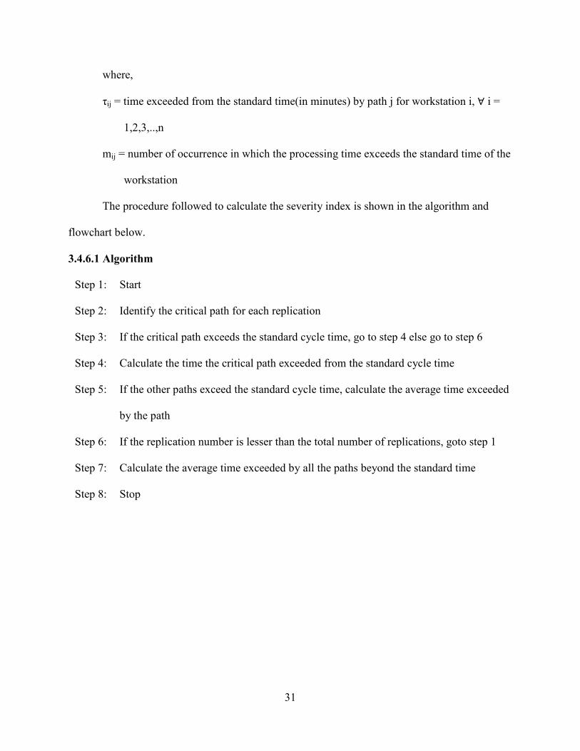
The procedure followed to calculate the severity index is shown in the algorithm and
flowchart below.
3.4.6.1 Algorithm
Step 1: Start
Step 2: Identify the critical path for each replication
Step 3: If the critical path exceeds the standard cycle time, go to step 4 else go to step 6
Step 4: Calculate the time the critical path exceeded from the standard cycle time
Step 5: If the other paths exceed the standard cycle time, calculate the average time exceeded
by the path
Step 6: If the replication number is lesser than the total number of replications, goto step 1
Step 7: Calculate the average time exceeded by all the paths beyond the standard time
Step 8: Stop

32
3.4.6.2 Flowchart

33
3.5 Case Study – 3 Workstation – 27 Processes
The methodology is verified using a case study which comprises of 3 workstations arranged in
line and each comprising of 9 processes. The processes involve machining and assembly
operations. The workstations are arranged in series layout as show in Figure 3.2.
Figure 3.2 Line diagram for the production system
The line diagram for a workstation is shown in the Figure 3.3.
Figure 3.3 Line diagram of workstation 1
The line diagrams for the second and third workstations are similar. Each workstation has
3 parallel paths and every path has 3 processes occurring in series. For a part to exit a
workstation, it needs to complete all the processes occurring within the workstation.
The processing time for each process follows triangular distribution for workstations 1, 2
and 3 which are shown in Tables 3.3(a), (b) and (c) respectively.

34
Table 3.3 (a) Processing times for workstation 1
Workstation 1 (i= 1)
Process 1 Process 2 Process 3
Path 1 (j=1) 1400,1550, 1650 1400,1448,1652 1402,1552,1653
Path 2 (j=2) 1370,1470,1700 1370,1471,1700 1470,1470,1700
Path 3 (j=3) 1350,1400,1750 1350,1400,1750 1350,1400,1750
Table 3.3 (b) Processing times for workstation 2
Workstation2 (i =2)
Process 1 Process2 Process3
Path 1 (j=1) 1400,1440,1650 1400,1550,1650 1400,1550,1650
Path 2 (j=2) 1370,1470,1700 1372,1468,1703 1372,1468,1698
Path 3 (j=3) 1350,1401,1749 1351,1399,1749 1348,1405,1748
Table 3.3 (c) Processing times for workstation 3
Workstation 3 (i= 3)
Process 1 Process 2 Process 3
Path 1 (j=1) 1401,1553,1657 1398,1551,1653 1401,1552,1648
Path 2 (j=2) 1371,1403,1752 1368,1401,1751 1368,1398,1753
Path 3 (j=3) 1351,1402,1753 1348,1398,1751 1351,1397,1748
All processing times are in minutes.

35
3.5.1 Deterministic case
If the data is assumed to be deterministic, path 1 is the critical path for all the
workstations. In order to produce the parts within the standard time of 4600 minutes, focus needs
to be given to path 1 for workstations 1, 2 and 3. Other paths need not be considered to improve
the line.
But in real cases, processing time is mostly stochastic and tends to follow some
distribution. The data obtained followed triangular distribution.
3.5.2 Stochastic case
Since the data followed a triangular distribution, the processing time for a particular line
is the sum of all the individual processes within the line. To calculate the critical path for each
time involved summing up for each line within a workstation leading to three distributions within
each of the workstation. Calculation of the summed distribution for the entire line leads to 27
different distributions. Thus, simulation was done.
The number of replications done is calculated using half width calculation as shown in
equation 3.11.
2
r 2
2α , n-12
N = h
tσ
3.11
Based on the half width analysis, and an H of ±17.5 minutes, the number of replications
required is 100. The simulation is done using discrete event simulation QUEST (QUeuing Event
Simulation Tool) software. Simulation is run for 6000 minutes. It is assumed that the task needs
to be completed within that workstation before the part is moved to the next workstation
irrespective of the move rate.

36
The number of parts produced per run is one. This case study is done for parts that have
high variability and low volume. Based on this, the average processing time per run was found to
be about 4619 minutes.
3.5.2.1 Critical path due to variability
Under deterministic conditions,path 1 is the critical path. However, due to variability all
the paths could tend to be a critical path for multiple runs. For the first workstation, the
probability that a path was a critical path is shown in Table 3.4. As seen in the table, path 1 has a
44% probability of being the critical path. However, path 2 has a 27% probability and path 3 has
a 29% probability.
Table 3.4 Critical path for workstation 1
So, emphasis needs to be given to path 1 for reducing the probability of path 1 being
critical. But, paths 2 and 3 can also be critical paths. If focus is given only to path 1 to reduce the
completion time, then paths 2 and 3 would become the critical path. The probability for a path
being critical for all the workstations is shown in Figure 3.4.
Path Probability of Critical Path
1 44 %
2 27 %
3 29 %

37
Figure 3.4 Probability of path being critical for all the workstations
One of the objectives is to successfully implement techniques to paths which may or may
not be critical paths all the time, so as to reduce the average processing run of 4619 minutes
closer to the expected move rate of the workstation with the available resources, such as man,
machine and money.
3.5.2.2 Critical path shift based on standard time
As discussed in the previous section, path 1 tends to be the critical path most of the time.
But, the standard time for each workstation is 4600 minutes. The previous method did not
consider whether the critical path exceeded the standard time. One of the objectives is to try to
reduce the total cycle time to the standard time of the workstation. So, emphasis is given only
when the total cycle time exceeds the standard time of the line. Based on the standard method,
paths that completed the process before 4600 minutes were not considered. Only the parts that
delayed beyond the standard time and the total time exceeded per path per runare considered.
0
10
20
30
40
50
60
Workstation 1 Workstation 2 Workstation 3
Path 1
Path 2
Path 3

38
3.5.2.3 Frequency beyond standard time
Critical paths that exceeded the standard cycle time are considered irrespective of the
time it exceeded the standard cycle time. The frequency of the standard cycle time exceeding the
standard cycle time is shown in Table 3.5.
Table 3.5 Frequency of a critical path exceeding the standard cycle time
Path number
No of times
exceeded
Percentage of Path being
critical
Probability that path is
critical and exceeding the
standard time
1 24 35% 24%
2 19 28% 19%
3 25 36.8% 25%
∑ 68%
The total number of times a critical path’s processing time exceeded the standard cycle
time is 68 times from the 100 replications. From the table, it can be inferred that the path one
again tends to be more critical. The probability of a critical path exceeding the standard time for
all the workstations is shown in Figure 3.5.

39
Figure 3.5 Probability of a critical path exceeding the standard time
Emphasis needs to be given on how much delay is caused by the critical path beyond the
standard time. This was calculated by summing up the difference in the actual processing time
for critical path and the standard cycle time. Based on that the total number of minutes the path
exceeded the standard move rate is calculated.
For example in replication 1 workstation 1,
replication 1
4695.2
(Critical Path) = max 4535.4
4467.6
Time taken by critical path = 4695.2
As the time taken at the critical path is greater than the standard time, that path is
considered.
A
no of times path 1 exceeded the standard timeP is the critical path =
no of occurences
24
*10068
=
0
5
10
15
20
25
30
35
40
45
Workstation 1 Workstation 2 Workstation 3
Path 1
Path 2
Path 3
Within standard time

40
= 35.3%
3.5.2.4 Critical path severity index (CSI)
The next step is to calculate the severity ratio, which is the ratio of the total number of
minutes a path exceeded the standard time and the number of times it exceeded for workstation i
and path j. The critical path severity index for path 1 for the first workstation is shown.
1
1742.238Critical path severity index for path 1 (α ) =
24
= 83.5
The severity ratios for paths 1 to 3 are shown in Table 3.6
Table 3.6 Critical path severity index for workstation 1
Path Total Exceeded Time (minutes)
No of times exceeded
Critical path severity index
(minutes)
Percentage contribution
(%)
1 2005.2 24 83.6 26.8
2 1953.2 19 102.8 32.9
3 3143.6 25 125.7 40.3
From the table, it can be inferred that the total number of times a critical path exceeds the
standard time is 24 (it is the summation of the number of times exceeded). The probability that a
critical path exceeds the standard time is 24%. The critical path severity index for all the
workstations are shown in Figure3.6.

41
Figure 3.6 Critical path severity indexes for all the workstations
From the graph, it is clear that the severity index for path 3 for all the workstations are
the maximum.
3.5.2.5 Severity index for all paths
The last section is focused on the difference in the time exceeded by all the paths from
the standard time. At times, paths other than the critical path could also exceed the standard cycle
time. This metric focuses not only on the critical paths that exceed the standard cycle time, but
also the non-critical paths that exceed the standard cycle time. The severity index for all paths for
workstation 1 is shown in Table 3.7.
Severity index for path 1 (β1) = 2663
39
= 68.3 minutes
0
20
40
60
80
100
120
140
160
180
Workstation 1 Workstation 2 Workstation 3
Path 1
Path 2
Path 3
42
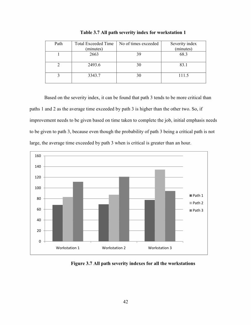
Table 3.7 All path severity index for workstation 1
Path Total Exceeded Time (minutes)
No of times exceeded Severity index (minutes)
1 2663 39 68.3
2 2493.6 30 83.1
3 3343.7 30 111.5
Based on the severity index, it can be found that path 3 tends to be more critical than
paths 1 and 2 as the average time exceeded by path 3 is higher than the other two. So, if
improvement needs to be given based on time taken to complete the job, initial emphasis needs
to be given to path 3, because even though the probability of path 3 being a critical path is not
large, the average time exceeded by path 3 when is critical is greater than an hour.
Figure 3.7 All path severity indexes for all the workstations
0
20
40
60
80
100
120
140
160
Workstation 1 Workstation 2 Workstation 3
Path 1
Path 2
Path 3

43
Table 3.8 Comparison of the Metrics
Metric Order of dominance
Probability of Critical Path 1-3-2
Based on move rate 1-3-2
Critical Path Severity Index 3-2-1
All path severity index 3-2-1
3.6 Conclusion
In this chapter, new critical path identification methods are proposed to help improve the
probability of completion of processes and measures such as critical path severity index, all path
severity index and critical path due to standard time are proposed. Various methods are used to
identify the critical path, such as what is the probability of a path being critical and the average
time a path exceeded the standard time. From the metrics, it can be inferred that path 1 for all the
workstations tends to be the critical path most of the time, although, when the average time a
path exceeds the standard cycle time is considered, path 3 tends to have a larger value with
respect to all the other paths for the workstations. Based on these methods, suitable suggestions
can be given to various lines for improvement. Methods to improve the line and allotment of the
improvement methods and the steps taken are suggested in the later chapters.

44
CHAPTER 4
LEAN IMPLEMENTATION
4.1 Introduction
The previous chapter explains about situations used to improve a production system
which has low volume and high variability scenarios such as an aircraft manufacturing industry.
Such industries have thousands of high variable operations occurring in series and in parallel.
Some tasks could either take a few minutes to complete or can also take several hours or days.
The variability is due to in availability of resources such as parts, labor and machines. In a
production system which has hundreds of operations, resources are needed in most of the
operations to reduce variability. But, due to limitations in cost and space, simply increasing
resources for all the variable operations is not feasible. The previous chapter talks about cases
where critical paths change over a period of runs due to variability and considers various metrics
that can be used to capture the variability of paths. This chapter focuses on using these metrics as
a tool to identify which improvement on which process will give the best results. Using this
technique, an industry will follow a systematic procedure for bringing an improvement and will
have control over the benefits of implementing an improvement technique. This will also help an
industry in tackling problematic processes based on a decreasing order of criticality.
4.2 Assumptions
The assumptions for lean implementation are
1. All lean experiments are independent of each other (the results of a lean tool on one
process would not change the results in another process).
2. Each process can undergo only one lean experiment.

45
3. Only one lean experiment can be implemented in one line.
4. The improvement can either be addition of extra labor, material or machinery.
4.3 Model input requirements
The proposed model requires the following input data for testing the lean implementation
approach:
1. Penalty cost for delay in parts
2. Precedence constraints in parts
3. Cost of lean experiments for all the workstations
4.4 Mathematical Model
Implementing the lean experiments would involve identifying the workstation with the
minimum probability of completion. Calculation of minimum probability of completion can be
done using equation 4.1.
i
j
c
# of simulation runs - # of times path j is critical and beyond standard time
P = # of simulation runs
∑ 4.1
After identifying the workstation with the least probability of completion, the next step is
to capture the worst path within that workstation. The formulation used to calculate the critical
path within a particular workstation is shown in equation 4.2.
critical path j for i = max (# of times j is critical and exceeds standard time
* average time exceeded) 4.2
Identifying the worst process would involve simulating the improvement on each process
and calculating the magnitude of improvement based on penalty cost. The process that shows the

46
maximum improvement is chosen for improvement. Equation 4.3 is used for calculating the
improvement on each process.
Improvement after lean for path j * penalty costImprovement for path j =
number of replications
∆ 4.3
The improvement for all the processes within the path is calculated using equation 4.3
and the maximum of the given values is chosen. The next step is to calculate the payback period
based on the cost of lean implementation which is shown in equation 4.4.
cost of lean implementationPay back period =
improvement for path j 4.4
After calculating the improvement in the workstation, repeat the simulation and identify
individual probability of completion and repeat the processes.
4.5 Case Study: High variability 3 workstations – 9 paths and 27 processes
The case study has been done on the 3 workstations, 9 paths and 27 process systems.
Each workstation has 3 paths that are in parallel. The paths are independent of each other. Each
path has 3 processes occurring in series and they are independent of each other. However, for the
part to move to the next workstation all the processes within the paths need to be completed.
Calculation of probability of critical path for each path is explained in the previous chapter. The
lean experiments for each path for all the processes are shown in table 4.1.
Each path has a unique improvement technique which has different costs to implement
and have different benefits. The improvement is reduction in processing time or reduction in the
variability.

47
Table 4.1 Cost of Lean Experiment and improvement
Lean experiment Reduction in time Cost to implement
1 (a-230,b-55,c-134) $ 160,000
2 (a-270,b-40,c-160) $ 240,000
3 (a-210,b-50,c-170) $ 150,000
4 (a-250,b-45,c-170) $ 200,000
5 (a-215,b-40,c-140) $ 155,000
6 (a-200,b-45,c-120) $ 115,000
7 (a-230,b-30,c-140) $ 175,000
8 (a-220,b-30,c-150) $ 100,000
9 (a-300,b-60,c-200) $ 300,000
The column reduction in time says that if lean experiment 1 is implemented, there would
be a reduction in the minimum value by 230 minutes, maximum value by 55 minutes and in the
mode by 134 minutes. Similarly, improvements from implementing the other lean experiments
can be obtained using the above table. Each of this experiment can be any improvement such as
adding men, equipment or improving the availability of raw material.
The first step is to identify the workstation with the least probability of competition.
Probability of completion is the probability that the workstation would complete the operation
within the standard time required to complete the given set of operations within that workstation.
The formulation for calculating the probability of completion is calculated from equation 4.1.
Probability of completion for workstation 1 is shown below.
1
100 31PC =
100
− = 69%

48
Similarly, probability of completion for each workstation is calculated and is shown in
figure 4.1. The probability of completion for the entire production system is the product of
probability of completion of individual workstations.
Figure 4.1 Probability of completion for all workstations
Attention is given to workstation 3 because of the minimum probability of completion of
64%. The next step is to identify the worst path in workstation 3. This is calculated as the
maximum of the product of the average time each critical path exceeds the standard move rate
(Metric 2) and the number of times the critical path exceeds the standard move rate (Metric 3).
This is calculated using table 4.2.
Table 4.2 Identification of the worst process
Metric 2 Metric 3
(in minutes)
M2*M3
Path 3 a 11% 45.1 496.54
Path 3 b 16% 92.6 1481.9
Path 3 c 10% 58.5 584.5
Based on the results shown in table 4.2, path 3 b is the worst path as it has the maximum
amount of time exceeded from the standard move rate. The final step is to calculate the process
that would be benefited the most with lean implementation, which is calculated by identifying
the maximum of the product of the reduction probability of critical path and the reduction in the
average time exceeded. The improvement for process is shown using equation 4.5.
P
c1 = 69% P
c2 = 67% P
c3 = 64 %
WS1 WS 2 WS 3
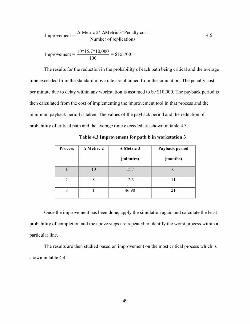
49
Metric 2* Metric 3*Penalty costImprovement =
Number of replications
∆ ∆ 4.5
10*15.7*10,000Improvement = = $15,700
100
The results for the reduction in the probability of each path being critical and the average
time exceeded from the standard move rate are obtained from the simulation. The penalty cost
per minute due to delay within any workstation is assumed to be $10,000. The payback period is
then calculated from the cost of implementing the improvement tool in that process and the
minimum payback period is taken. The values of the payback period and the reduction of
probability of critical path and the average time exceeded are shown in table 4.3.
Table 4.3 Improvement for path b in workstation 3
Process ∆ Metric 2 ∆ Metric 3
(minutes)
Payback period
(months)
1 10 15.7 6
2 8 12.3 11
3 1 46.98 21
Once the improvement has been done, apply the simulation again and calculate the least
probability of completion and the above steps are repeated to identify the worst process within a
particular line.
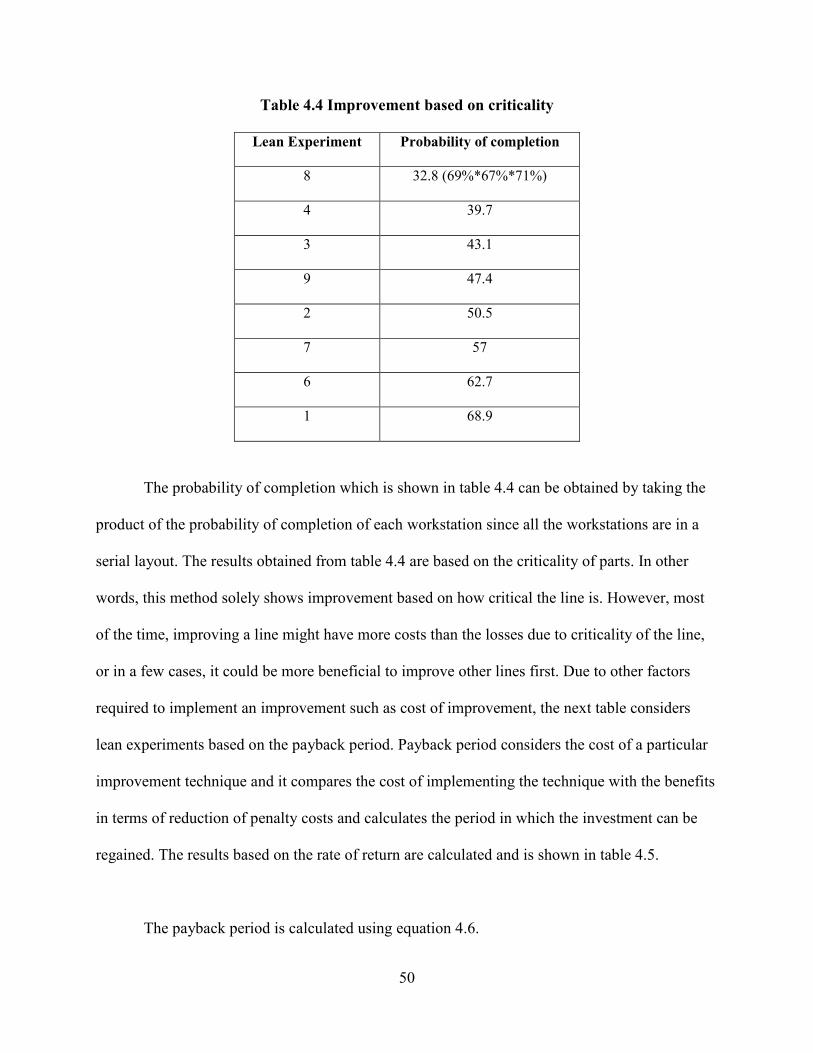
The results are then studied based on improvement on the most critical process which is
shown in table 4.4.
50
Table 4.4 Improvement based on criticality
Lean Experiment Probability of completion
8 32.8 (69%*67%*71%)
4 39.7
3 43.1
9 47.4
2 50.5
7 57
6 62.7
1 68.9
The probability of completion which is shown in table 4.4 can be obtained by taking the
product of the probability of completion of each workstation since all the workstations are in a
serial layout. The results obtained from table 4.4 are based on the criticality of parts. In other
words, this method solely shows improvement based on how critical the line is. However, most
of the time, improving a line might have more costs than the losses due to criticality of the line,
or in a few cases, it could be more beneficial to improve other lines first. Due to other factors
required to implement an improvement such as cost of improvement, the next table considers
lean experiments based on the payback period. Payback period considers the cost of a particular
improvement technique and it compares the cost of implementing the technique with the benefits
in terms of reduction of penalty costs and calculates the period in which the investment can be
regained. The results based on the rate of return are calculated and is shown in table 4.5.
The payback period is calculated using equation 4.6.

51
Cost of implementing the improvementPay back period =
Re duction in penalty cost per month 4.6
For calculating the payback period for the path a at workstation 3
Table 4.5 Lean implementation based on payback period
Lean Experiment Payback period(months)
4 3
7 5
6 5
9 7
8 6
3 7
2 10
1 21
Table 4.5 explains about selection of lean experiment based on the payback period for
each improvement technique. This chapter proposes a methodology of applying improvements
either by just considering the criticality of each path. It also helps identify a method to apply
improvements by considering the costs to implement an improvement by considering the
payback period.
100,000Pay back period for workstation 3 path b = = 7 months
15,700

52
CHAPTER 5
STUDY OF CRITICAL PATH BASED ON VARIABILITY
The previous chapters showed methods to identify critical paths and implement
improvements based on cost of implementation and rate of return on investment. The study was
done for high variability conditions. This chapter studies the effect of the proposed methodology
for improving the line based on changes in variability. In the previous chapter, the analysis was
done on high variability scenarios. This chapter aims to study the effect of improving the line,
with lesser levels of variability.
5.1 Variability Levels
The various levels of variability that were studied are follows:
Case 1: no variability in the system
Case 2: low variability in the system
Case 3: medium variability in the system
The cases are set based on the initial case study. For example, consider the distribution for
process 1 for workstation 1 at path 1 which is shown in figure 5.1 A. For the first case, the mean
of the distribution is considered as the processing time. In the second case, the minimum is one
third of the difference in the minimum and the mode. Similarly, the maximum is one third the
difference in the maximum and the mode which is shown in figure 5.1 B. The third case is
similar to the second case except that two third the difference is considered which is shown in
figure 5.1C.

53
Figure 5.1 A High variability
Figure 5.1 B Low Variability
Figure 5.1 C Medium Variability
Figure 5.1 Distributions for process 1 in line 1 for workstation 1
5.2 No variability
In the no variability case, the processing time was taken as the mean processing time and
based on this,the critical path was calculated. Critical path was identified to be only one line per
workstation and there was no shift in the critical path within workstations. Similarly, there was
no difference between the probability of a path being critical and the probability a critical path
1450 1550 1616
1500 1550 1583
1400 1650 1550

54
exceeding the standard move rate. Metrics which are used to study the criticality of each path
that is explained in the third chapter are shown in table 5.1.
Table 5.1 Critical path analysis for deterministic case
WS 1 WS 2 WS 3
Metric 1
Path 1 100% 100% 100%
Path 2 0% 0% 0%
Path 3 0% 0% 0%
Metric 2
Path 1 100% 100% 100%
Path 2 0% 0% 0%
Path 3 0% 0% 0%
Metric 3
Path 1 150 250 256
Path 2 0 0 0
Path 3 0 0 0
Metric 4
Path 1 150 250 256
Path 2 11 6 12
Path 3 0 0 0
There is no change in the critical path in the deterministic case. Hence, lean experiments
were implemented without any further simulation which is shown in table 5.2.

55
Table 5.2 Order of Lean Experiments in Deterministic case
Lean Experiment Probability of Completion
6 0
2 0
8 73.6%
1 83.7%
5 94%
9 100%
The probability of completion was found to be zero, since all three workstation had a
mean processing time greater than standard move rate. Hence, lean experiments were
implemented on all three workstation in order to observe any improvement in the probability of
completion. However, only six lean experiments were required to increase the probability of
completion and the processes were done within the standard move rate. This case is ideal,
wherein there is no variability in the system. Though this is impractical, two cases with different
levels of variability were studied.
5.3 Low variability case
After studying the deterministic case, the next step was to increase the variability. The
variability was around one third of the high variability case. The metrics required to identify the
criticality of each path were calculated. Lean experiments were implemented to the paths based
on criticality based on the methodology which is shown in chapter 3.
Table 5.3 Critical path analysis for low variability case

56
WS 1 WS 2 WS 3
Metric 1
Path 1 92% 100% 100%
Path 2 8% 0% 0%
Path 3 0% 0% 0%
Metric 2
Path 1 10% 85% 94%
Path 2 1% 0% 0%
Path 3 0% 0% 0%
Metric 3
Path 1 8.7 46.1 48.0
Path 2 14.9 0 0
Path 3 0 0 0
Metric 4
Path 1 8.7 46.1 48.0
Path 2 14.9 15.1 12.2
Path 3 0 0 0
After identifying the metrics, the next step was to calculate the order in which the lean
experiments need to be done in order to improve the probability of completion which is shown in
table 5.4.
Table 5.4 Order of Lean Experiments in less variability scenario

57
Lean Experiment Probability of Completion
6 11.5%
2 60.5%
8 64.5%
1 69.8%
5 73.5%
9 81.9%
Like the deterministic case, only six lean experiments were required to increase the
probability of completion and the processes were done within the standard move rate.
5.4 Medium variability case
The study was also done in the medium variability scenario. The steps involved are
similar to the previous cases. The criticality of each path for all the workstations is shown in
table 5.5.
The results that were obtained from table 5.5 are similar to the high variability case.There
is a shift in the criticality of paths, wherein the more variable path has a lesser probability of
being critical. However, when it is critical, the average time exceeded is large.
The order of lean experiments and the probability of completion are shown in table 5.6.
Table 5.5 Critical path analysis for medium variability case
WS 1 WS 2 WS 3

58
Metric 1
Path 1 54% 56% 60%
Path 2 33% 21% 22%
Path 3 13% 23% 18%
Metric 2
Path 1 22% 31% 38%
Path 2 27% 16% 15%
Path 3 11% 19% 17%
Metric 3
Path 1 29.8 24.6 25.8
Path 2 45.8 39.2 34.7
Path 3 54.3 59.7 63.7
Metric 4
Path 1 15.6 17.4 17.6
Path 2 37.4 32.6 29.9
Path 3 45.1 52.6 51.2
Table 5.6 Order of Lean Experiments in medium variability scenario
Lean Experiment Probability of Completion
8 25.7%
4 33.5%
3 40.8%
9 52.5%
2 56.3%
7 60.1%
6 65.8%
1 82.3%
Table 5.7 shows the lean experiments for all the cases based on probability of
completion. These results do not take the cost of applying the lean experiment into consideration.
Table 5.7 Order of lean experiments based on probability of completion

59
The results show that there is no significant difference in the medium and the high
variability case.
Table 5.8 shows the lean experiments for all the cases based on return on investment.
This table takes the cost of applying each experiment and the improvement from each
experiment into account.
Table 5.8 Order of lean experiments based on payback period
Deterministic Less variability Medium variability High variability
9 9 4 4
5 5 6 7
8 4 7 6
4 8 8 8
1 1 9 9
2 2 2 3
1 2
3 1
There is no significant difference in the order of experiments for the medium variability
and the high variability case. The results shown in table 5.8 is similar to the results in table 5.7
stating that there is not much variation in the medium and high variability scenarios. However,
there is a significant difference in the order of lean experiments for the order of experiment based
Deterministic Less variability Medium variability High variability
6 6 8 8
2 2 4 4
8 8 3 3
1 1 9 9
5 5 2 2
9 9 7 7
6 6
1 1

60
on the probability of completion and the payback period. By comparing the results, it can be
inferred that the most critical path may not be the best path to improve due to the cost of
implementing. It also states that the cheapest improvement may not have ideal results due to
significance of the criticality of the path. Based on the study on different levels of variability, it
can be inferred, that the shift in the critical path is more in the medium and the high variability
cases. In such cases alone, simulation is a key tool that can be used to study the effects on critical
path. In the less variability case, simulation need not be done

61
CHAPTER 6
CONCLUSION AND FUTURE RESEARCH
6.1 Conclusion
In this section, the conclusion and future research for this study is discussed. For products
that are manufactured which have high variability in processing times and manufactured in low
volume, improvement cannot be just given to the line that takes the maximum processing time.
Due to different levels of variability within each process, different processes might be critical at
different runs. Various metrics are used to study the paths and analyze the criticality of multiple
paths. The metrics used to capture the criticality of paths for high variable production systems
such as aircraft manufacturing industries are shown in chapter 3. After identifying the criticality
of paths, a systematic procedure for improvement is discussed about in chapter 4. Different
improvement techniques have different costs. The improvement techniques could be addition of
labor, increasing machinery or improving the availability of material. Improvements are based on
either to improvement in the probability of completion or based on return on investment.
Chapter 5 discusses about implementing the proposed methodology for different levels of
variability. It shows the results of implementing critical path using simulation for different levels
of variability.
In order to improve a production system which has high variability and low volume,
improvement on the path which has the highest processing time alone will not yield significant
results. Improvement needs to be given to the process that has high variability and a significant
processing time. In order to identify that process various metrics were used. The tool used to
identify these metrics was simulation. The metrics used were based on the processing time and

62
the variability. By combining the various metrics, a method was shown to identify the paths that
caused delays in production. Once the various critical paths were identified, the next step was to
identify a procedure for improvement. Various improvement techniques were allotted for each
process. Each improvement technique could either be allocating extra personnel, machine or
increasing buffer before the process. The improvements were used to either reduce variability or
processing time or a combination of both. Each improvement technique has a unique cost for
implementation. Implementing improvement techniques were based on the costs to implement
and the criticality of the path.
6.2 Future Research
The research brings into account different levels of variability and considers different
cost factors for different experiments. However, only one improvement could be used for each
process. At times, more than one improvement could be necessary for a process. Besides, having
more than one improvement technique for a process could increase flexibility in applying
improvement techniques. One of the factors for implementing an improvement technique was
considering the improvement to be independent of each other. Though most of the time, an
improvement technique could either have a positive or a negative effect on other lines. When the
problem becomes larger, simulating a model gets tedious and time consuming. Genetic algorithm
or other heuristic methods can be used to solve problems which require a lot more operations to
save time and resources.

63
REFERENCES

64
REFERENCES
Achanga, P., Shebah, E., Roy, R. (2006), “Critical success factors for lean implementations within SMEs”, Journal of Manufacturing Technology Management, Vol. 17, No. 4, pp.460-471. Buckley, J, J. (1989), “Fuzzy PERT: Applications of fuzzy set methodologies in industrial engineering.” Elsevier, Amsterdam, pp. 103-114 Chanas, S. (1989), “Fuzzy sets in few classical operational research problems.” Approximate
Reasoning in Decision Analysis, Amsterdam, pp.351-363 Chanas, S., Kamburowski, J. (1981), “The use of fuzzy variables in PERT”, Fuzzy Sets and Systems, Vol. 5, pp. 1-19 Chanas, S., Radonsinski, E. (1976), “A model of activity performance time in the light of fuzzy set theory”, Problemy Organizacji, (in Polish) Vol. 2, pp. 68-76 Chang, I, S., Tsujimura, Y., Gen, M., Tozawa, T. (1995), “An efficient approach for large scale project planning based on fuzzy Delphi method”, Fuzzy Sets and Systems Vol. 76, pp.277-288 Chanas, C., and Zielinski, P. (2000), “Critical path analysis in the network with fuzzy activity times.” Fuzzy Sets and Systems, Vol.122. pp. 195-204. Durgaparameswaran, K. “A study of variability in aircraft assembly lines”. MS Project. Wichita State University, 2010. Print Ginzbufg, D, G. (1988), “On the distribution of activity time in PERT” Journal of Operations
Research Society, Vol. 39, No. 8, pp. 767-771. Hoffmann, P, A. (1991), “Critical path method: An important tool for coordinating clinical care.” Journal of Quality Improvement, Vol. 19, No. 7, pp. 235-246 Hopp, W, J., and Spearman, M, L., Factory physics: Foundations of manufacturing management (3rd edition), NY: Irwin/McGraw-Hill, 2001, English. Malcolm, D, G., Roseboom, J, H., Clark, C, E., Fazar, C, W. (1959), “Application of a technique for research and development project evaluation”, Operations Research Vol. 7, pp. 646-669 Mucklow, J,C., Fraser, H, S., Bulpitt, J., Kahn, C., Mould, G., and Dollery, C, T. (1980), “Environmental factors affecting paracetamol metabolism in London factory and office workers”, Journal of Clinical Pharmacol, Vol.10, No. 1, pp.67-74 Nasution, H, S. (1994), “Fuzzy critical path method.” IEEE transactions of systems, man and
cybernetics. Vol. 24, No.1, pp. 48-57

65
Pachaimuthu, S., S. “Risk based worker allocation and line balancing”. MS thesis. Wichita State University, 2010. Print. Prade, H. (1979), “Using fuzzy sets theory in a scheduling problem: a case study”, Fuzzy Sets and Systems, Vol. 2, pp. 153-165. Rommelfanger, H. (1994), “Network analysis and information flow in fuzzy environment”, Fuzzy Sets and Systems, Vol. 67, pp. 119-128. Schoderbek, P,P. (1965), “A study of the applications of PERT” The Academy of Management
Journal, Vol. 8, No. 3, pp.199-210 Shtub, A. and Dar-El, E. (1999), “An analytic frameworks for sequencing mixed model assembly lines”, International Journal of Production Research,Vol. 30, No.1, pp 35. Slyeptsov, A, I., Tyshchuk, T, A. (1997), “Fuzzy critical path method for project network planning and control”, Cybernet System Analysis, Vol. 3, pp.158-170. Suer, G. (1996), “Optimal operator assignment and cell loading in labor intensive manufacturing cells.” Computer and Industrial Engineering, Vol. 31, No. ½, pp. 155-158 Wickwire, J, M. and Smith, R, F. (1975), “The use of critical path method techniques in contract claims.” Pub. Cont. L. J. Winston, L, W. Operations Research: Applications and Algorithms. Belmont, CA. Duxbury Press, 1994. English. Yamin, R, A., & Harmelink, D. J. (2001), “Comparison of linear scheduling model (LSM) and critical path method (CPM).” Journal of Construction Engineering and Management, Vol. 127, No. 5, pp. 374-381 Yao, J, S., Lin, F, T. (2000), “Fuzzy critical path method based on signed distance ranking of fuzzy numbers”, IEEE Transactions Systems Man Cybernet, Vol.20, pp. 76-82. Zhang,X.,Bi,E.,Novick,P.,Du,L.,Kozminski,K.G.,Lipschutz,J,H.,Guo,W. (2001), “Cdc 42 interacts with the expcyst and regulates polarized secretion”, Journal of Biological Chemistry,Vol. 276, pp.46745-46750