automated cnc tool path planning and machining simulation
TRANSCRIPT

Clemson UniversityTigerPrints
All Dissertations Dissertations
5-2013
Automated CNC Tool Path Planning andMachining Simulation on Highly ParallelComputing ArchitecturesDmytro KonobrytskyiClemson University
Follow this and additional works at: https://tigerprints.clemson.edu/all_dissertations
This Dissertation is brought to you for free and open access by the Dissertations at TigerPrints. It has been accepted for inclusion in All Dissertations byan authorized administrator of TigerPrints. For more information, please contact [email protected].
Recommended CitationKonobrytskyi, Dmytro, "Automated CNC Tool Path Planning and Machining Simulation on Highly Parallel Computing Architectures"(2013). All Dissertations. 1779.https://tigerprints.clemson.edu/all_dissertations/1779

AUTOMATED CNC TOOL PATH PLANNING
AND MACHINING SIMULATION ON HIGHLY
PARALLEL COMPUTING ARCHITECTURES
A Dissertation
Presented to
the Graduate School of
Clemson University
In Partial Fulfillment
of the Requirements for the Degree
Doctor of Philosophy
Automotive Engineering
by
Dmytro Konobrytskyi
May 2013
Accepted by:
Dr. Laine Mears, Committee Chair
Dr. Thomas R. Kurfess
Dr. Tommy Tucker
Dr. Stan Birchfield

ii
ABSTRACT
This work has created a completely new geometry representation for the
CAD/CAM area that was initially designed for highly parallel scalable environment. A
methodology was also created for designing highly parallel and scalable algorithms that
can use the developed geometry representation. The approach used in this work is to
move parallel algorithm design complexity from an algorithm level to a data
representation level. As a result the developed methodology allows an easy algorithm
design without worrying too much about the underlying hardware. However, the
developed algorithms are still highly parallel because the underlying geometry model is
highly parallel.
For validation purposes, the developed methodology and geometry representation
were used for designing CNC machine simulation and tool path planning algorithms.
Then these algorithms were implemented and tested on a multi-GPU system.
Performance evaluation of developed algorithms has shown great parallelizability and
scalability; and that main algorithm properties are required for modern highly parallel
environment. It was also proved that GPUs are capable of performing work an order of
magnitude faster than traditional central processors.
The last part of the work demonstrates how high performance that comes with
highly parallel hardware can be used for development of a next level of automated CNC
tool path planning systems. As a proof of concept, a fully automated tool path planning
system capable of generating valid G-code programs for 5-axis CNC milling machines

iii
was developed. For validation purposes, the developed system was used for generating
tool paths for some parts and results were used for machining simulation and
experimental machining. Experimental results have proved from one side that the
developed system works. And from another side, that highly parallel hardware brings
computational resources for algorithms that were not even considered before due to
computational requirements, but can provide the next level of automation for modern
manufacturing systems.

iv
TABLE OF CONTENTS
Page
TITLE PAGE ....................................................................................................................... i
ABSTRACT ........................................................................................................................ ii
LIST OF TABLES ........................................................................................................... viii
LIST OF FIGURES ........................................................................................................... ix
LIST OF ALGORITHMS ................................................................................................ xvi
CHAPTER
I. INTRODUCTION ........................................................................................................... 1
Importance of automated tool path planning ...................................................................... 2
Importance of parallel processing ....................................................................................... 4
The proposed approach for solving automated milling problem ........................................ 6
The role of this work in the proposed automated milling framework ................................ 9
Work structure .................................................................................................................. 15
II. BACKGROUND AND RELATED WORK ................................................................ 17
CNC milling ...................................................................................................................... 17
Geometry representation ................................................................................................... 19
Milling simulation ............................................................................................................. 23
Parallel processing and GPGPU ....................................................................................... 25

v
Table of Contents (Continued)
Page
GPU architecture and OpenCL ......................................................................................... 28
III. 3-AXIS MACHINING SIMULATION ...................................................................... 35
Height map representation of a machined workpiece ....................................................... 36
Workpiece rendering ......................................................................................................... 39
Generalized cutter representation for 3-axis milling simulation ....................................... 43
3-axis milling simulation algorithm .................................................................................. 44
Experimental 3-axis simulation results ............................................................................. 49
Milling simulation and rendering performance ................................................................ 53
Accuracy analysis ............................................................................................................. 62
Discussion ......................................................................................................................... 66
IV. TOOL PATH PLANNING FOR 3-AXIS MACHINING .......................................... 69
GPU accelerated 2d contour offset roughing path planning algorithm ............................ 70
Tree based algorithm for path components connection optimization ............................... 75
GPU accelerated shifted zigzag finishing path planning algorithm.................................. 80
Experimental 3-axis path planning and milling results ..................................................... 84

vi
Discussion ......................................................................................................................... 87
V. 5-AXIS MACHINING SIMULATION ....................................................................... 89
Table of Contents (Continued)
Page
Geometry representations and data structures evaluation ................................................. 90
Developed irregularly sampled volume representation .................................................... 95
Tool motion representation for 5-axis milling simulation .............................................. 102
5-axis milling simulation based on irregularly sampled volume .................................... 107
Irregularly sampled volume rendering algorithm ........................................................... 115
Accuracy analysis ........................................................................................................... 124
Experimental 5-axis simulation results ........................................................................... 128
Simulation performance analysis .................................................................................... 135
Discussion ....................................................................................................................... 148
VI. TOOL PATH PLANNING FOR 5-AXIS MACHINING ........................................ 150
Parallel algorithms design methodology ......................................................................... 153
Volume based parallel algorithms design methodology and limitations ........................ 155
Offset volume calculation ............................................................................................... 157

vii
Surface filling algorithm based on 3D contour offset approach ..................................... 167
Robust tool trajectory generation for 5-axis machines ................................................... 172
Orientation selection ....................................................................................................... 176
Accessibility map generation .......................................................................................... 196
Table of Contents (Continued)
Page
High level tool path planning control algorithm ............................................................. 205
Experimental 5-axis milling results ................................................................................ 205
Discussion ....................................................................................................................... 210
VII. CONCLUSIONS AND RECOMMENDATIONS .................................................. 212
REFERENCES ............................................................................................................... 215

viii
LIST OF TABLES
Table Page
I-1: Fastest CPU and GPU performance ........................................................................... 13
V-1: Geometry representations comparison ..................................................................... 95
V-2: Cell value changes .................................................................................................. 110
V-3: GPUs parameters .................................................................................................... 136
V-4: Base performance results ........................................................................................ 136
VI-1: Test models properties for offset volume calculation ........................................... 161
VI-2: Offset volume calculation performance results ..................................................... 161

ix
LIST OF FIGURES
Figure Page
I-1: History of milling machines ......................................................................................... 1
I-2: Processor clock frequency over time [2] ...................................................................... 5
I-3: Tool path planning iteration ......................................................................................... 7
I-4: Tree of possible path planning decisions ..................................................................... 8
II-1: BREP example [34] .................................................................................................. 20
II-2: Triangular mesh example [34] .................................................................................. 20
II-3: CSG example [35] .................................................................................................... 21
II-4: Octree example [36] .................................................................................................. 22
II-5: Quad-tree height map example ................................................................................. 23
II-6: OpenCL platform model ........................................................................................... 30
II-7: OpenCL memory model. .......................................................................................... 31
II-8: OpenCL threads grid ................................................................................................. 32
III-1: 1D height map ......................................................................................................... 39
III-2: Height map rendering example ............................................................................... 41
III-3: Cutting tool intersection .......................................................................................... 43
III-4: Cutting tool height map representation ................................................................... 44
III-5: Height map updating process - before editing ......................................................... 45
III-6: Height map updating process - editing .................................................................... 45
III-7: Height map updating process - after editing ............................................................ 46

x
List of Figures (Continued)
Figure Page
III-8: Collision example .................................................................................................... 48
III-9: Test model “Tiger paw” .......................................................................................... 49
III-10: Test model “Yoda” ................................................................................................ 50
III-11: Test model “Zoo” .................................................................................................. 51
III-12: Test model “Sculptures” ........................................................................................ 52
III-13: CPU vs. GPU simulation performance .................................................................. 54
III-14: Performance vs. Group size (global size = 8k)...................................................... 56
III-15: Performance vs. Global size .................................................................................. 56
III-16: Effect of collision avoidance on performance ....................................................... 57
III-17: Simulation performance vs. Global size with CPU ............................................... 58
III-18: Rendering vs. Resolution....................................................................................... 59
III-19: Simulation components vs. Resolution ................................................................. 60
III-20: OpenCL-OpenGL interoperability improvement .................................................. 61
III-21: Cutter parts description.......................................................................................... 62
III-22: Difference between actual and interpolated radiuses ............................................ 63
III-23: Cutter interpolation error based on points number ................................................ 64
III-24: Cutter error based on position ............................................................................... 64
IV-1: Part slices................................................................................................................. 71
IV-2: Contour offset .......................................................................................................... 71
IV-3: Iterative roughing tool path ..................................................................................... 72
xi
List of Figures (Continued)
Figure Page
IV-4: Slicing test part ........................................................................................................ 76
IV-5: Not optimized tool path ........................................................................................... 77
IV-6: Generated tree ......................................................................................................... 77
IV-7: Optimized tool path ................................................................................................. 78
IV-8: Tree optimization testing result ............................................................................... 79
IV-9: Tool offset ............................................................................................................... 81
IV-10: Distance between tool and target surfaces ............................................................ 82
IV-11: Required testing points. ......................................................................................... 82
IV-12: Height map generation with zigzag 2d path .......................................................... 83
IV-13: Experimental milling results for the “Tiger paw” model ...................................... 85
IV-14: Experimental milling results for the “Sculptures” model ..................................... 86
IV-15: Experimental milling results for the “Yoda” model .............................................. 86
IV-16: Experimental milling results for the “Zoo” model ................................................ 87
V-1: Developed geometry representation model .............................................................. 99
V-2: 2D example of the developed model surface representation .................................... 99
V-3: HDT hierarchy ........................................................................................................ 100
V-4: Developed geometry model from a memory point of view .................................... 101
V-5: Generalized tool model [62] ................................................................................... 103
V-6: Ball-end tool swept volume model ......................................................................... 106
V-7: Multi GPU load balancing ...................................................................................... 108

xii
List of Figures (Continued)
Figure Page
V-8: Machining simulation process shown on 2D geometry model............................... 111
V-9: Threads distribution during subcells editing .......................................................... 113
V-10: Nodes memory management model ..................................................................... 115
V-11: Two height map generation iterations used for rendering .................................... 117
V-12: Curve represented by spherical cells .................................................................... 118
V-13: Curve represented by spherical subcells ............................................................... 119
V-14: Rays casted from each pixel on a screen plane .................................................... 120
V-15: Estimated surface and normals ............................................................................. 121
V-16: Rendering results .................................................................................................. 123
V-17: Demonstration of dark borders around foreground objects .................................. 123
V-18: Tolerances for multiple tolerance grades [64]. ..................................................... 126
V-19: 3-axis model “Sculptures” (new 5-axis simulator on the right) ........................... 129
V-20: 3-axis model “Zoo” (new 5-axis simulator on the right) ...................................... 130
V-21: 5-axis machining simulation process for model “Puppy” .................................... 131
V-22: 5-axis machining simulation process for model “Fan” ........................................ 132
V-23: 5-axis machining simulation process for model “Fan” ........................................ 133
V-24: Simulation result for model “Dragon”.................................................................. 133
V-25: Roughing process of the “Teapot” model............................................................. 134
V-26: Various simulation results .................................................................................... 134
V-27: Machining test setup ............................................................................................. 135

xiii
List of Figures (Continued)
Figure Page
V-28: Editing time vs. Resolution .................................................................................. 139
V-29: Performance vs. Available computing power ....................................................... 140
V-30: Utilization of available computation power ......................................................... 141
V-31: Performance vs. Step size ..................................................................................... 142
V-32: Rendering speed vs. Resolution............................................................................ 143
V-33: Frame rendering time vs. Resolution .................................................................... 144
V-34: Rendering time vs. Zoom level............................................................................. 145
V-35: Rendering speed vs. Available computing power ................................................ 146
V-36: Rendering speed vs. GFLOPS (w/o constant time) .............................................. 147
V-37: Available computing power utilization ................................................................ 148
VI-1: Offset surface [65] ................................................................................................. 158
VI-2: Offset surface self-intersections [66] .................................................................... 158
VI-3: 2D offset surface decomposition ........................................................................... 159
VI-4: Offset volume generation performance ................................................................. 162
VI-5: “Teapot” volume offset ......................................................................................... 163
VI-6: “Turbine” volume offset........................................................................................ 164
VI-7: “Candle holder” offset volume .............................................................................. 165
VI-8: “Head” offset volume. ........................................................................................... 166
VI-9: Curve offsetting ..................................................................................................... 169
VI-10: Iterative surface area filling................................................................................. 170

xiv
List of Figures (Continued)
Figure Page
VI-11: Restriction volume for the “Head” model ........................................................... 171
VI-12: Surface filling for finishing tool path generation ................................................ 173
VI-13: Initial curve selection for roughing process ........................................................ 174
VI-14: Layer by layer material removing during a roughing process. ........................... 175
VI-15: Accessibility map example.................................................................................. 177
VI-16: 3D curve going through a stack of bitmaps......................................................... 179
VI-17: Example of a tool trajectory that requires a tool retraction ................................. 180
VI-18: Dependency of a jump point on tool movement direction .................................. 180
VI-19: A scenario with a complicated tool space topology ............................................ 181
VI-20: Two possible ways of orientation selection ........................................................ 181
VI-21: Accessibility space .............................................................................................. 182
VI-22: Explanation of an accessibility map construction process .................................. 183
VI-23: “Jump” concept explanation ................................................................................ 184
VI-24: Accessibility space slicing and connection ......................................................... 185
VI-25: Graph representation of an accessibility space ................................................... 186
VI-26: Real life example of an accessibility map graph ................................................. 188
VI-27: Curve representation ........................................................................................... 191
VI-28: 3D curve optimization example .......................................................................... 193
VI-29: Accessibility space (views from multiple camera positions) .............................. 194
VI-30: Accessibility curve going through accessibility space, view 1 ........................... 195

xv
List of Figures (Continued)
Figure Page
VI-31: Accessibility curve going through accessibility space, view 2 ........................... 195
VI-32: Accessibility curve going through accessibility space, view 3 ........................... 196
VI-31: Touching a cell surface by a tool surface ............................................................ 197
VI-32: Touching a sphere from multiple sides ............................................................... 198
VI-33: All tool orientation when a tool touches a sphere ............................................... 199
VI-34: 2D tool model ...................................................................................................... 200
VI-35: Inaccessibility cone angle components ............................................................... 201
VI-36: Test model “Head” .............................................................................................. 208
VI-38: Test model “Puppy” ............................................................................................ 209

xvi
LIST OF ALGORITHMS
Algorithm Page
III-1: Height map rendering .............................................................................................. 40
III-2: Material removing simulation ................................................................................. 47
III-3: Material removing simulation second approach ...................................................... 47
IV-1: Edge detection ......................................................................................................... 73
IV-2: Edge expansion ....................................................................................................... 74
IV-3: Continuous path construction .................................................................................. 75
IV-4: Tree optimization .................................................................................................... 79
IV-5: Finishing path planning ........................................................................................... 84
V-1: First part of the machining simulation process ....................................................... 109
V-2: Second part of the machining simulation process .................................................. 109
V-3: Rendering................................................................................................................ 122
VI-1: Belonging test ........................................................................................................ 153
VI-2: Belonging test for machining simulation .............................................................. 153
VI-3: Volume surface intersection .................................................................................. 154
VI-4: Volume offset calculation ..................................................................................... 160
VI-5: Surface filling ........................................................................................................ 171
VI-6: Finishing tool path generation ............................................................................... 172
VI-7: Roughing path planning ........................................................................................ 174
VI-8: Accessibility graph construction ........................................................................... 187

xvii
List of Algorithms (Continued)
Algorithm Page
VI-9: Initial accessibility curve construction .................................................................. 190
VI-10: Accessibility curve optimization ......................................................................... 192
VI-11: Accessibility map calculation.............................................................................. 203
VI-12: High level control algorithm ............................................................................... 205

1
I. INTRODUCTION
During the last century the manufacturing industry has moved from pure manual
or simple mechanically automated production of goods to a new level where almost
everything is controlled by electronic control systems and computers. Although areas like
assembling or repairing are still done mostly by people, it is almost impossible to see
large scale manual mechanical processing today mainly due to the requirements of
precision, repeatability and speed. In order to meet the increasing requirements of
produced components, the way of controlling machine tools evolved from manual
operation to mechanical control systems during 19th
century, then to Numerical Control
(NC) systems in the middle of 20th
century and finally to Computer Numerical Control
(CNC) systems (Figure I-1).
Figure I-1: History of milling machines
Modern CNC machines are extremely versatile in their ability to make parts with
complex geometry and good surface quality. However, efficient usage of all machine
capabilities requires highly experienced personnel and a relatively long time to program.

2
The main reason it requires tremendous time investments is a lack of efficient and
flexible automatic path planning algorithms and, as a result, a lack of reliable, fast and
fully automatic software for CNC programming. Existing algorithms are usually limited
to specific problem solutions due to the geometric and computational complexity of path
planning. In addition, existing algorithms cannot be run efficiently on modern, highly
parallel hardware for utilization of modern computing capacity and as a result are limited
to performance of traditional serial processors.
Importance of automated tool path planning
It is hard to underestimate the importance of the further automation of the milling
process and especially of automated tool path planning. Although modern Computer
Aided Manufacturing (CAM) systems have significantly simplified the process of
machine programming, creating a program for an average part still takes several hours.
As a result, the cost of low volume production when only few parts are required may
consist mainly of a programming cost. For example, in an extreme case of one part
milling, which is a popular mold and die manufacturing scenario, programming cost may
be 90% of the entire manufacturing cost. This extremely high cost of low-volume
production with CNC milling is also one of the main reasons that subtractive
manufacturing is not used in Rapid Prototyping (RP) industry. The RP industry is almost
monopolized by a variety of additive manufacturing techniques today which usually do
not require such complicated programming process. As a result, development of highly
automated path planning systems could create a completely new market for RP by CNC

3
milling, which would provide a unique combination of cost, speed, precision and ability
to use production materials. It is obvious that decreasing prototyping cost is extremely
important for an entire manufacturing industry, due to shorter product development life
cycle and much cheaper testing.
It may look like the high programming cost is important only for low volume
production and not for high volumes where a programming cost is shared between
millions of parts. This is partially true and actual milling time is much more important in
this case, but usually designing of an optimal trajectory, which does take as little time as
possible, is not a trivial problem and requires multiple iterations. In this case automated
tool path planning may significantly improve a tool path planning iteration time and
allow a significantly higher number of iterations with a much shorter resulting tool path.
In an extreme case of fully automated tool path planning and simulation, these tool path
planning iterations can be performed without human assistance in a cloud by thousands
of servers with a much more efficient result than a human can ever achieve.
The importance of automated path planning is also proved by a survey [1] that
was conducted online in March and April of 2010 among 188 machine tool professionals
by Centrifuge Brand Marketing Inc. and sponsored by Siemens Industry, Inc. The survey
showed that 81% of job shops and 72% of manufacturers are looking for faster
programming and setup; and 74% of job shops and 70% of manufacturers are looking for
easiness of use for reduced training time, which is one of the benefits of automated tool
path planning.
4
Importance of parallel processing
Automatic tool path planning is obviously an important research area for modern
manufacturing industry and there many research projects have been conducted on this
subject in the past few decades. The “Background” chapter will provide more detailed
information about past research projects, but it is important to notice that all tool paths
planning today is done by computers and that path planning algorithms are becoming
more and more complicated and require more computational resources. It is also
important to notice that until a very recent time, tool path planning and simulation
algorithms could be designed quite independently from knowledge about the hardware
that actually performs them, and all algorithms were serial. This approach was good
enough for the early stage of the computer industry when new processors were always
faster than old processors and algorithm developers could expect seeing better
performances of their algorithms every year. This state of continuous performance
improvement was possible mainly because of the increasing of Central Processing Unit
(CPU) and memory clock frequencies. But increasing clock frequency also means higher
heat production and further increasing of a clock frequency creates physical limitations
that become more and more complicated for processor manufacturing.
At the beginning of 2000’s further increasing of a clock frequency had become
too expensive from the heat production point of view and the decision made by processor
manufacturers was to use multiple CPU cores and single-instruction, multiple-data
(SIMD) processors with a lower frequency in order to increase the available
computational performance for the next generations of their processors. The power
5
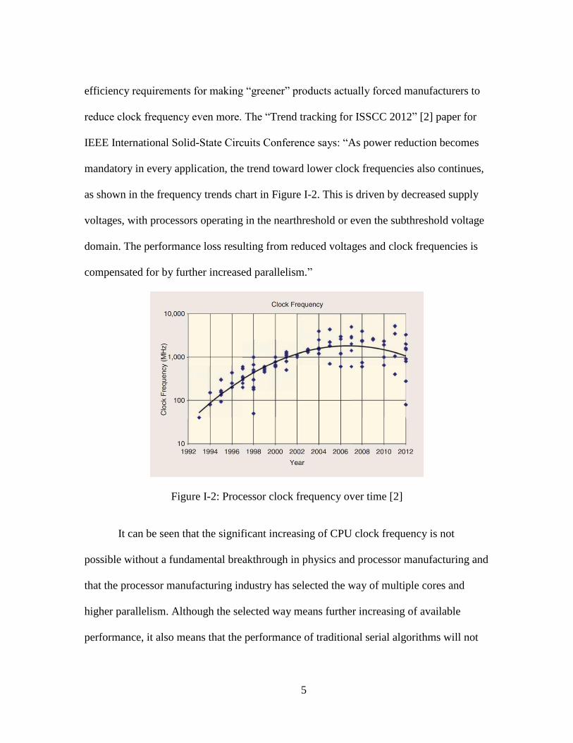
efficiency requirements for making “greener” products actually forced manufacturers to
reduce clock frequency even more. The “Trend tracking for ISSCC 2012” [2] paper for
IEEE International Solid-State Circuits Conference says: “As power reduction becomes
mandatory in every application, the trend toward lower clock frequencies also continues,
as shown in the frequency trends chart in Figure I-2. This is driven by decreased supply
voltages, with processors operating in the nearthreshold or even the subthreshold voltage
domain. The performance loss resulting from reduced voltages and clock frequencies is
compensated for by further increased parallelism.”
Figure I-2: Processor clock frequency over time [2]
It can be seen that the significant increasing of CPU clock frequency is not
possible without a fundamental breakthrough in physics and processor manufacturing and
that the processor manufacturing industry has selected the way of multiple cores and
higher parallelism. Although the selected way means further increasing of available
performance, it also means that the performance of traditional serial algorithms will not

6
increase significantly anymore. As a result, algorithm developers cannot expect seeing
continuous computational time improvement for traditional algorithms anymore and will
be required to develop new parallel algorithms using modern hardware.
The proposed approach for solving automated milling problem
Previous parts have shown the importance of automatic tool path planning for the
manufacturing industry and also the importance of parallel processing as a critical
component for any high performance algorithms. This work proposes a high level
approach for solving both problems in terms of automated CNC tool path planning and
provides a foundation for further research and development of this solution.
The global problem of the manufacturing industry (and many other industries as
well) today is an absence of a centralized knowledge base with information about milling
processes, materials, path planning strategies and good practices. Although the industry
has already found solutions for many problems, there is still no way for automated
selection, applying and evaluation of these solutions. Traditionally the knowledge about
milling processes and path planning strategies is shared between independent CNC
programmers and cannot be reused without actual interaction with people, implemented
though CAM systems User Interface (UI). At the same time CAM packages already have
multiple tool path planning strategies implemented and there are existing tool and
material properties databases, which can be used for covering most of everyday milling
needs.

7
It is also obvious that there is no way to put all of the available knowledge of all
CNC engineers, CAM developers and tool and material properties databases into one
place immediately. The proposed solution is to develop a centralized system, which can
be continuously improved in an iterative way by adding new knowledge about path
planning strategies, tools, materials and machines on each iteration. Although it may look
like the proposed approach is just to create a knowledge data base, the key component of
the proposed solution is to develop a software system that can actually use this
knowledge for solving tool path planning problems automatically. The proposed system
would perform 5 main steps as shown on Figure I-3:
1) Feature detection
2) Tool path planning strategy selection
3) Tool path planning with selected strategy strategies
4) Simulation
5) Performance evaluation
Figure I-3: Tool path planning iteration
There are multiple ways to use the proposed approach. One way is to apply these
steps iteratively with optimization of path planning parameters on each step as is usually
done in tradition optimization problems. Another way is to actually make a tree of all (or
all of the most probable) decisions made at the second step for each detected feature and
Feature detection
Strategy selection
Trajectory generation
SimulationPerformance
evaluation

8
process a tree by generating a tool path and simulation of each decisions sequence as
shown on
Figure I-4.
Figure I-4: Tree of possible path planning decisions
Evaluation of every generated tool path for a tree can be done by simulation of
milling process and collecting some measurements like path length, milling time, tool
load, material removing rate and even tool and workpiece temperatures. The results of
this evaluation can be processed for selection of the best tool path, based on user defined
criteria like the fastest milling time or the most efficient tool wear or the maximum
scallop height. As with path planning strategies, tool path evaluation would have a
modular structure and could be extended by adding new evaluation algorithms.
The proposed solution is significantly different from any modern CAM system in
the way that it is initially fully automated and becomes better over time by continuously
accumulating knowledge about path planning strategies, simulation and tool path
evaluation techniques.

9
The role of this work in the proposed automated milling framework
Although an implementation of the proposed solution is obviously not simple, and
it is more of a computer engineering and organizational problem than a research problem,
there are some fundamental scientific problems that have to be solved in order to actually
develop the proposed system.
One of the main problems is the need of a very robust algorithm which can be
applied to any possible geometry and produce a valid tool path. One of the reasons for
this need is an ability to generate a tool path at the beginning of system development
when there are no tool path planning algorithms. Another more general reason is a
requirement for robustness of the proposed system. It can be seen that on one side the
number of implemented feature detection and path planning algorithms will grow up and
cover more and more path planning scenarios and possible geometries. But on another
side there are no guaranties that the available algorithms can always produce a valid
output tool path for any provided input geometry. It means that the proposed system will
be able to generate useful output only for a subset of all the problems and that the number
of problems that can be solved will be relatively small at the beginning of development.
One of possible solutions for this problem is described in this work. The idea is to
develop a robust multi-axis tool path planning algorithm, which can be applied for any
possible geometry and produce a reasonably optimal valid tool path. This algorithm does
not have to be extremely efficient or fast but the most important quality for it is to be able
to produce a valid tool path for any input geometry if it is feasible from a geometry point
of view. The proposed automated tool path planning system would use this algorithm as a

10
last resort in cases where there are no known efficient algorithms for selected features or
where there are no detected features. Based on the idea of continuous improvement it is
obvious that this algorithm will be used more often at the beginning of development and
less often after adding more efficient algorithms. The algorithm developed in this work
fits the desired requirements and will be described in further chapters.
Another important fundamental problem is related to parallel processing. As
described above, parallel processing has become a main processor industry trend and
there are no known solutions that can allow further growing of CPU clock frequency and
the increasing of serial algorithms’ performances without a significant breakthrough in
physics, material science and processor manufacturing. As a result, even in 10-20 years
current serial algorithms will not become much faster. But this is only one side of a
problem. On the other side, performance of modern CAM systems is barely good for
everyday usage i.e. it is possible to perform multiple tool path planning generation
iterations for relatively simple geometry or few iterations for complex geometry in a
reasonable time (some hours), but there is no way to use the same algorithms for the
hundreds and thousands of tool path planning iterations required for the proposed
automated tool path planning system. And although multi-core processors have been
available on the market already for 8 years, modern CAM systems still have very limited
support of parallel processing, which usually requires a user to run multiple independent
tasks manually. In the case of 2-cores it still can be a reasonable solution but with modern
6- and 8-core processors it becomes extremely inefficient.

11
The reason for the absence of parallel processing support in modern CAM
systems is related to the way geometry is represented. Traditionally Computer Aided
Design (CAD) and CAM systems use boundary geometry representation (BREP)
developed back in 1970s. The BREP has a lot of advantages that were extremely
important during the second part of 20th
century; especially the support of extremely high
accuracy with relatively low computational and memory requirements. It provides the
best set of tradeoffs between accuracy, memory usage and required amount of
calculations on a serial processor for most geometry operations required by CAD and
CAM systems. Although BREP is a good geometry representation, it has some significant
drawbacks that are becoming more important today with spreading of multi-core
processors. One important drawback of BREP is the complexity of geometry operations
from a human point of view. Even reasonably simple operations like Boolean subtraction
or an intersection between a plane and a compound surface represented by BREP require
a lot of complex mathematical calculations which usually cannot be represented as a set
of simple independent operations. This drawback has two important results: the
development of CAM systems becomes quite complicated with BREP and it is not
possible to use data parallelism for parallel processing support. The data parallelism and
its comparison to task parallelism will be given in the “Background” chapter but the main
difference is related to how work is divided between multiple cores. In case of data
parallelism it is quite easy to split work between many cores without significant effort
from a developer. In opposition to data parallelism, task parallelism requires developers
to split work manually, which is a much more complicated problem, especially for a high

12
number of cores. For example one of the most popular geometric modeling kernels used
in modern CAD/CAM systems called “Parasolid” has recently started support “thread-
safety” which means that developers can run multiple editing tasks on multiple cores.
And although it is definitely a good trend, development of software systems, which can
really use many cores, with manual load balancing requires a tremendous effort and
usually cannot be done in a research environment.
The idea behind a solution for the parallel processing problem is actually quite
simple: use another geometry representation, which provides a different set of tradeoffs
between memory consumption, computational requirements and accuracy but supports
parallel processing on data level and can be scaled efficiently. This work presents results
of the research project about automated tool path planning and also results of a search for
a new geometry representation, which can efficiently replace a traditional boundary
representation and solve existing parallel processing problems. Since the BREP is a good
tradeoff between accuracy, memory, computational requirements, complexity and
scalability, it is easy to assume that in order to reduce complexity and improve scalability
another geometry representation may take more memory and/or computational resources
for the same level of accuracy. At the same time the facts are that modern processors are
barely fast for CAM systems using traditional BREP and performance of CPUs is
growing quite slow. Five years ago, it appeared that there was no way to solve the
problem. Now, it seems to be the same way - but the solution has actually come from the
gaming industry.

13
One of the most important aspects of games is the quality of the graphics. In order
to render images faster, the computer graphics industry starting in the 1980s has been
using specialized hardware called Graphics Processing Units (GPU). In the early stages
of computer graphics and gaming industries, GPU was just a chip with some predefined
rendering algorithms implemented in the hardware. But the gaming industry required
more realistic graphics and more flexibility of hardware implemented algorithms. As a
result, at the beginning of the 2000s GPU had gotten the support of special programs
called shaders written by software developers in addition to predefined hardware
algorithms. Increased flexibility requirements forced GPU manufacturers to make their
processors more and more general and as a result it has become possible to do General
Purpose calculation on GPU (this approach is called GPGPU). More information about
GPU architecture, GPGPU approach and GPU performance will be given in the
“Background” chapter but it is important to notice 2 things: GPU is a naturally highly
parallel and theoretical GPU performance is a several hundred times higher than serial
CPU performance. For example theoretical performance of the fastest modern CPU and
GPU is shown in Table I-1. It can be seen that the theoretical performance difference
between serial programs and parallel programs that use SIMD approach on CPU is 81x
and parallel programs on GPU is almost 1500x faster than serial programs on CPU.
Processor name Performance (SP GFLOPS)
Intel i7-3960X (Serial performance @ 3.9GHz) 3.9
Intel i7-3960X (Parallel SIMD performance @ 3.3GHz) 316
NVidia GTX690 (Parallel performance) 5621
Table I-1: Fastest CPU and GPU performance
14
The shown theoretical possibility of performance improvement in the case of
parallel algorithms proves that parallel processing is a crucial part of any modern
software system. It can also be seen that a transition from serial CPU algorithms to
parallel algorithms, which can run on GPU, may provide a performance improvement
comparable to the past 30 years of continuous CPU performance growing. The GPU
actually may provide the additional computational resources needed in the case of new
geometry representations which will replace BREP and add support of parallel
processing. Although it may look like GPU is a perfect solution and that all modern
software should run on it, the difference in CPU and GPU architectures does not allow a
simple porting of algorithms from one platform to another. More details about
architectural differences and GPU algorithm design challenges will be given in the
“Background” chapter but it is important to notice that in order to achieve theoretical
performance limits, algorithms and data structures have to be designed especially for
GPU and, in most cases, this is not a trivial problem. The current research actually
provides the geometry representation including data structure and algorithms especially
designed for highly parallel GPU architectures, which supports data parallelism and
allows performing of all operations in parallel without a significant effort from a
developer. Data parallelism means that the development of parallel tool path planning
algorithms is significantly easier and developed algorithms can scale even to multi-GPU
systems as will be shown later.

15
Work structure
This work describes the research of algorithms, data structures and geometry
representations that can be used for efficient milling process simulation and tool path
planning accelerated by GPGPU approach. The information is provided in approximately
chronological order, so that the research path and key decisions made during the research
project can clearly be seen. All required background information about CNC milling,
parallel processing and GPGPU approach is provided in the “Background” chapter,
which also describes past research in the milling area and gives information about
modern GPU architectures required for understanding GPU algorithms development
challenges. The entire work is divided in two main areas: 3-axis milling and 5-axis
milling. Although 3-axis milling can be described as a subset of 5-axis milling, the
approach used for 3-axis tool path planning and simulation is similar and allows easier
showing of some important concepts of GPU accelerated milling before going to 5-axis.
The entire research can also be divided into two other areas: milling simulation and path
planning, which may look like independent areas, but it will be shown that generalized
tool path planning approach cannot be implemented without integration of tool path
planning and milling simulation algorithms into one system. As result of this double
subdivision, 4 main structures of this work are “3-axis milling simulation”, “Tool path
planning for 3-axis milling”, “5-axis milling simulation”, “Tool path planning for 5-axis
milling” that correspond to described research areas. The chapter “Conclusion and
recommendation” at the end provides a summary of the entire research and describes

16
future research possibility of the developed technology. The last part of this work
provides references to books, papers and other resources used in this work.

17
II. BACKGROUND AND RELATED WORK
CNC milling
CNC milling has progressed in the last 40 years from fully mechanical machine
controls, punch cards and paper tapes to modern fully computerized controllers,
programmed via variants of G-code programming languages. Programming these
machines has advanced from inefficient handwritten programs to powerful CAM systems
capable of generation complex multi-axis trajectories, based on strategies selected by
operator and precise virtual milling simulation.
Significant research has been focused on key areas such as tool path planning,
tool orientation selection, and selection of tool geometry. Many researchers have
addressed tool path planning using traditional methods such as iso-planar [3-5] or iso-
parametric approaches [6]. Results of these approaches generate paths that achieve
certain accuracies, or surface characteristics, but that may not be optimal with respect to
other process parameters, such as production time. In order to improve performance of
traditional methods, the iso-scallop approach was introduced by Suresh and Yang [7] and
Lin and Koren [8]. It produces a constant scallop height of a machined surface.
Popularization of 5-axis milling and milling of non-parametric surfaces has resulted in
the development of new approaches resolving specific 5-axis problems and further
reducing milling time. These approaches can be classified [9] as curvature matched
milling [10-12], isophote based method [13-15], configuration space methods [16, 17],

18
region based tool path generation [13], compound surface milling [18, 19] and methods
for polyhedral models and cloud of point [20, 21]. With respect to tool orientation
selection, traditional methods such as fixed orientation, principal axis methods [22] or
multi point milling [23] have been developed. Furthermore, in the past 10 years, more
advanced path planning methods such as the rolling ball [24, 25] and arc intersect
methods [26] as well as earlier C-space based approaches [16, 27] were successfully
deployed. Furthermore, research addressing tool geometry selection [28, 29], and
implementation of automatic tool selection in commercial products does not exist or is
very limited when addressing optimized tooling parameter selections. While significant
progress has been achieved over the last several decades, a plethora of issues to be
addressed that will reduce production time and improve / guarantee component quality
still exist.
Throughout the literature, it is clear that computation time is a major limitation of
most, if not all, of the proposed algorithms. One solution for this problem is the
employment of high performance computing, in particular the GPU (Graphical
Processing Unit) platform to accelerate the processing. Development and popularization
of a general purpose GPU (GPGPU) approach and platforms like Compute Unified
Architecture (CUDA) have resulted in promising results for deploying GPGPU
functionality in a manufacturing environment. Tukora and Szalay presented an approach
for GPGPU accelerated cutting force prediction [30]. Hsieh and Hsin proposed a GPU
accelerated particle swarm optimization approach for 5-axis flank milling [31].
Furthermore, new approaches for geometry representation used in CNC area were

19
recently proposed. Guang and Ding proposed employing a quadtree-array for
representation of a workpiece in 3-axis milling [32]. Li and Yao used an extended octree
for cutting force prediction. Zhao and Wang presented a GPU accelerated approach for
Boolean operations on polygonal solids. Wang and Leung described the use of layered
depth-normal images for solid modeling of polyhedral objects [33]. All of this research
demonstrated the value of parallelized processing in milling operations.
Geometry representation
One of the most fundamental concepts in the CAD/CAM area is the geometry
representation. There are several fundamentally different approaches for representing
geometry such as Boundary Representation (b-rep or BREP), Constructive Solid
Geometry (CSG), volume sampling, height map, sweeping, implicit representation and
other approaches. Many of them have multiple implementations based on different data
structures such as arrays, lists or trees and unit elements such as voxels, surfaces, planes
or triangles. Traditionally modern CAD/CAM systems use solid modeling engines based
on BREP but also support other techniques such as CSG or sweeping volumes. In
opposition to CAD/CAM world, the game and art industries usually work with triangular
meshes since they provide a different set of tradeoffs which is more appropriate for these
applications.
The BREP approach uses limits for representing a shape. It represents a boundary
between material and empty space by a set of connected surface elements. Surface
elements are usually represented by NURBS (Non-uniform rational B-spline) surfaces or

20
by other analytical surface descriptions. In additional to geometric data the BREP stores
topological information including faces (bounded portion of a surface), edges (bounded
portion of a curve) and vertexes as shown on Figure II-1.
Figure II-1: BREP example [34]
A special case of a BREP, where all faces are planes, is called a polygonal mesh.
The triangular mesh can be described as a special case of BREP as well or as a polygonal
mesh where all faces are represented by a set of triangles as shown on Figure II-2.
Figure II-2: Triangular mesh example [34]

21
The triangular mesh representation is widely used in computer graphics and can
be rendered extremely quickly and efficiently by Graphics Processing Units (GPUs).
In opposition to BREP the CSG approach uses Boolean operations between
simpler objects in order to create a complex solid. The CSG approach does not require
storing additional topological information but the pure CSG approach can represent a
limited set of shapes. As a result it is usually used in combination with BREP approach
which is used for describing CSG primitives.
Figure II-3: CSG example [35]
One approach that is completely different from BREP is representing a volume
itself, and not a boundary surface. Volumetric approaches usually subdivide an entire
space into smaller areas called voxels or cells. Every volumetric element stores volume
sampling data which may contain information such as material density, distance to the
closest surface, color or something also. Based on volume subdivision, it is possible to
notice two ways of sampled approaches: regularly and irregularly. This way of

22
subdivision also affects a selected data structure used for storing sampling data. For
example, a regularly sampled volume data is usually stored in 3-dimensional arrays (this
geometry representation is called “voxel model” and volume elements are called
“volumetric pixels” or “voxels”). In case of irregularly sampled volume data, tree-like
data structures are usually used for as a storage, for example Octree (Figure II-4) or k-d
tree.
Figure II-4: Octree example [36]
Geometry representations described above provide different tradeoffs between
precision, memory usage, parallelization and complexity but they are very general
purpose and can represent any possible shape. In contrast to them, the height map
geometry representation is not capable of representing any possible geometry but
provides an interesting set of tradeoffs and can be useful in tasks like 3-axis milling (with
some limitations which will be mentioned later). The height map (or z-map) represents a
surface by storing sampled distances from a base plane to points of a represented surface.
The distance sampling data can be stored in a 2d array or a tree-like structure such as
quad-tree as shown on Figure II-5.

23
Figure II-5: Quad-tree height map example
Milling simulation
Milling simulation today is a critical component of the milling process that allows
safe usage of machines, prevents collisions, saves material and also allows the selection
of better milling parameters. Many researchers have being working in this area since the
1980s and have developed several different simulation techniques. It is important to
notice some of the most popular approaches described in published works.
In the earliest days of milling simulation area and limited computational resources
Boolean operations on solids was a main simulation tool. For example in 1983 Bertok
and Takata [37] used it for the prediction of a cutting torque and in 1986 Tim Van Hook
[38] described a system for rendering a solid milled by a cutting tool following an NC
path. Usage of Boolean operations on a solid has the benefit of producing a very accurate
result and a perfect image with low computational requirements for a small number of
tool motions. The drawback of this approach, however, is a dependency on the number of

24
operations required for image rendering on a number of tool motions which can be very
high in real NC programs.
In opposition to Hook in 1993, Hsu and Yang [39] used an isometric projection
and a height map data structure for 3-axis real-time milling simulation. This approach
guarantees an independency of rendering performance from a number of tool motions
although it provides only an approximate result with a predefined resolution and does not
provide a natural way for multi-axis simulation. Although as Roth and Ismail [40]
showed in 2003 it is possible to use a height map for multi-axis milling by the continuous
generation of height maps for each tool orientation. A different solution based on the
single voxel model for representing a workpiece was presented in 2000 by Jang and Kim
[41]. The concepts of primitives voxelization process similarly used by Jang and Kim
was published earlier in 1997 by Cohen-Or and Kaufman [42].
One of the crucial components for all described methods is the calculation of the
swept volume of a tool. One of the first papers on swept volume calculation was
published by Wang and Wang [43] in 1986. A newer approach for the APT tool was
described by Bohez and Minh [44] in 2003. Although all mentioned that simulation
approaches are quite different and use different data structures, almost all of them are
pure geometric simulation techniques.
Another class of milling simulation is an actual physical simulation with the finite
element method described in the work of Ozel and Tugrul [45] in 2000 and in the newer
work of Rai and Xirouchakis [46] published in 2008. Although the finite element
approach provides a much more accurate simulation and allows the measurement of

25
many physical parameters like tool temperature or tool load, it has two important
problems. The first problem is a need of physical parameters of material, tool and
machine which are not always available and may be hard to measure. Another problem is
related to a computational time. Modern processors cannot achieve even a real-time
simulation with a relatively coarse grid, which makes finite element simulation a useless
tool for manufacturing and limits its use to scientific research projects.
It is important to notice that most of the latest researches related to milling
simulation lies in areas like error prediction and compensation, like the work of Uddin
and Ibaraki [47] published in 2009 or Cortsen and Petersen [48] published in 2012, web-
based simulation described in the work of Hanwu and Yueming [49] published in 2009,
unification of manufacturing resources description proposed by Vichare and Nassehi [50]
published in 2009, and quad-tree-array based workpiece representation used in the work
of Li and Ding [32] published in 2010.
Parallel processing and GPGPU
It is well known that most popular computer processors as we see them today
were developed in 1980s, and since that time there were two main sources of increasing
their performance: growth of clock frequency which directly increases performance
because it allows performing more operations per second; and growth of transistor
number and circuit complexity which allows performing more complicated commands
and many commands per clock cycle. It is also well known that the physical limitations
of existing manufacturing processes and processor technologies do not allow further

26
significant increasing of a clock frequency and increasing number of transistors in a
processor becomes more and more complicated as well. Since increasing the clock
frequency is not an option anymore and it may be impossible to continue increasing
transistors number soon, at least without a significant breakthrough, it is important to
look at other possible ways of increasing available computational performance which
mainly lies in the area of more efficient usage of existing resources.
In order to understand how to use existing resources efficiently, it is important to
understand that tradeoffs have to be solved by processor developers, which is basically
how to use available transistors. In general, for a given number of transistors there are
two extreme ways to resolve a main tradeoff: make a processor that can perform one very
complicated command per clock cycle; or make a processor that can perform many very
simple commands per clock cycle. In the real world all existing processors are
somewhere in between. For example the Central Processing Unit (CPU), used for
performing most operations in modern computers, can perform few complicated
commands per clock cycle (and actually can perform a few times more simple
commands) and Graphics Processing Unit (GPU), used for 3d graphics calculations, can
perform many relatively simple commands per clock cycle. It is interesting that new
generation of CPUs can perform more and more commands per clock cycle and new
generations of GPUs can perform more complicated commands with fewer limitations, so
both CPUs and GPUs are becoming closer from an architecture point of view.
Although the tradeoff described in the previous paragraph is not just one and there
are many other tradeoffs related to memory subsystem, branch prediction, command

27
scheduling and others, the described one is one the most fundamental and important.
Based on this explanation it is easy to see that CPU is more generally purposed and more
algorithms may achieve good performance since CPUs can perform more complicated
commands specific for each algorithm and algorithms actually do not need to provide
many commands for each clock cycle. In opposition to this situation, GPU can perform
only simple commands and only algorithms which use simple commands and can
perform many commands at the same time will achieve high performance. What is even
more important is that these algorithms will run on GPU much faster than on CPU. This
situation makes sense since CPU is designed for any possible applications like browsers,
games, video players, scientific applications, engineering applications and all have to
achieve good performance. GPU, however, is designed specifically for 3d graphics that
require many simple independent math calculations. Although a GPU may perform only
specialized tasks, these tasks running on GPU may achieve hundreds times faster
performance than they would running on CPU (for example modern desktop CPU may
perform up to 4 billion floating point operations per second (or 4 GFLOPS) for serial
algorithm or up to 192 GFLOPS for highly optimized parallel algorithms and GPU may
perform up to 5621 GFLOPS for GPU-optimized algorithm) and an attempt to get similar
performance boost for all applications is a goal of General Purpose calculations on GPU
(GPGPU) technology which allows running general purpose applications on GPU.
Although GPGPU may look like a great solution for all performance problems, it
only allows running non-graphics code on GPU, but does not change its architecture.
Now developers have to find a way to use GPU hardware more efficiently. The main

28
problem here is how to provide enough commands to GPU on every clock cycle. In the
case of serial processing on CPU only one command of algorithm is given on every clock
cycle, which is exactly how all algorithms are usually designed. In the case of GPU,
hundreds or even thousands of commands have to be given and these commands have to
be independent from each other because they will be performed concurrently or in
parallel. This becomes a problem since usually the commands in algorithms use results of
previous commands and process data continuously. In order to solve this problem new
algorithms and data structures for representing processing data have to be selected or
developed that allow issuing many independent commands every clock cycle and
somehow combining results of their work and designing especially for GPGPU purpose.
GPU architecture and OpenCL
The previous part describes the importance of parallel processing and the tradeoff
that processor manufacturers have to resolve. Although the need of highly parallel
algorithms is the main result of using highly parallel architectures for GPUs it is not the
only one. The GPU memory and work scheduling subsystems are also significantly
different from their CPU analogs and this difference has to be considered in an algorithm
design phase since inefficient memory usage and significant control path branching result
in extremely high performance penalties in opposite to traditional CPUs. In order to
understand how to design efficient GPGPU algorithms it is important to understand the
architecture of modern GPUs that perform these algorithms and available development
tools and concepts.

29
Before going into discussion of GPU architectures it is also important to notice
that there are three major GPGPU platforms on the market today: CUDA from NVidia
[51], DirectCompute from Microsoft [52] and OpenCL from Khronos Group [53]. The
CUDA is a proprietary NVidia technology that works only on NVidia GPUs. It was the
first commonly used GPGPU technology mainly because it was a result of a significant
and successful effort to make a GPGPU development easier. In opposition to CUDA,
OpenCL was developed by Khronos group as an open standard for heterogeneous
computing that may work on many possible devices with different architectures. At the
current moment all major processor manufacturers have added OpenCL support and
released OpenCL SDKs for their processor which means that it is possible to run the
same code on several different platforms. Although an ability to write the same code for
different devices may significantly simplify a development process the significant
difference between architectures requires optimization of code for each architecture or
even device separately. The Direct Compute is the latest technology developed by
Microsoft as a part of DirectX that supposed to compete with OpenCL. In order to
popularize DirectCompute and make it easier to use there was developed the C++ AMP
extension that allows running C++ code with minor changes on GPU. For this work the
OpenCL was selected since it is an open standard supported by all major chip makers
which may become a main standard used for GPGPU computing in future. The OpenCL
programming language is based on C99 standard. It adds the additional concept of a
kernel – functions running on GPU, memory spaces corresponding to different physical
memory locations and some other features which allow access hardware resources.

30
In this work almost all algorithms were implemented in OpenCL and run on
GPUs with NVidia Fermi architecture, and this platform will be discussed (all values will
be given for NVidia GeForce GTX580). Although there are some major differences
between NVidia, AMD and Intel GPU architectures most of the concepts and ideas
behind GPU architectures design are the same and this discussion can be generalized to
all available GPUs.
From the OpenCL [54] point of view every computing system contains a set of
Compute Devices (CD) which are GPUs in case of GPGPU technology used in this
research; every Compute Device contains a set of Compute Units (CU) which are
Streaming Multiprocessors in used CUDA architecture and every Compute Unit contains
a set of Processing Elements (PE) which are CUDA cores as shown on Figure II-6.
Figure II-6: OpenCL platform model
For example one of the computing systems used in this research had 3 Compute
Devices (2x GeForce GTX580 and 1x Quadro 6000) with total number of 46 Compute
Units and total of 1472 Processing Elements.

31
At the same time from the memory model point of view there are Global,
Constant, Local and Private Memory spaces as shown on Figure II-7. Global and
Constant memories are physically allocated in GPU memory which has a relatively high
throughput (~200Gb/s) but very high latency (~800cycles), although Constant memory
has an additional cache which allows efficient reading of the same value by multiple
threads. The Local memory is physically stored inside of GPU chip and every CU has
access to an individual Local Memory storage. This memory type has much lower latency
(~10cycles) and relatively high bandwidth (~1Tb/s) but the size of it is very limited
(~48Kb/CU). The Private memory is the fastest available data storage which represents
CU registers which are divided by all PE and only accessible by one PE. In modern
GPUs there is also available L2 cache (768Kb/CD) used for caching Global memory
access and part of Local memory storage is used for L1 cache (16Kb/CU).
Figure II-7: OpenCL memory model.

32
From the programming point of view GPU processes a grid or N-Dimensional
Range (with up to 3 dimensions) of Work Items as shown on Figure II-8 where all Work
Items are combined into N-Dimensional work groups.
Figure II-8: OpenCL threads grid
For each work item, GPU launches a light-weight thread that performs a selected
function called “kernel”. Since the number of command schedulers on each Compute
Unit is much less than a number of Processing Elements, multiple PEs are combined in a
group (32 elements) called “warp” (“warp” is the term used by NVidia, AMD uses the
term “wavefront” for their architecture, that actually has value 64) and all PEs in this
group perform the same command on different work item data elements. This approach is
called SIMD (Single Instruction, Multiple Data) and it allows development highly
parallel processors which can process many data elements per clock cycles. The
important drawback of this approach is a significant penalty in the case of code
33
branching, it is easy to see that if some threads in a warp follow one branch of code and
other follow another branch they have to wait for each other since they can perform only
one command at a time. This drawback means that efficient algorithms need to have a
low control flow divergence inside warps.
Another important limitation of GPUs is related to the high global memory
latency which can be up to a thousand clock cycles. In order to hide this latency GPU
runs much many threads that it can process at a time and switches between them in order
to process available data while other threads are waiting for loading data. It means that a
number of running threads has to be much higher than a number of processing elements
in order to hide GPU memory latency and this number may need to be as high as tens of
thousands in opposite to few threads on CPU.
The last limitation to be mentioned is also related to a memory subsystem. As it
was mentioned before, physical limitations do not allow significantly increasing clock
frequency for modern processors but the same limitations affect also memory chips and
memory manufacturers need to use a workaround. One of the most popular ways is
similar to processor technologies – use parallel processing or parallel reading/writing in
case of memory. In order to achieve high throughput required for GPU many data
elements or words are loaded from or stored to memory in one memory access operation.
Usually it is implemented in the way that a linear block of words is accessed in one
memory operation (this is a limitation of a memory controller complexity) and the
number of words is equal to number of threads in a warp so each warp thread can read or
write a word in one memory command. This approach works quite well and allows

34
achieving extremely high memory bandwidth, but only if all threads access a continuous
block of memory. If threads access words at completely random memory addresses this
process is serialized and multiple memory access commands are issued which results in a
significant performance penalty.
The described list of three GPU architecture limitations is not a full list, but even
they can reduce performance by many orders of magnitude. In order to understand the
importance of optimization and GPU specific algorithm and data structure design it may
be useful to look on the difference between most efficient and most inefficient programs
from the described limitations point of view. The code branching limitation can reduce
the program up to 32X if all threads follow different branches, the linear memory access
limitation may also result in up to a 32X slower performance if all memory commands
have to be issued 32 times. Memory latency limitation may result in up to 800X slower
performance if processors have to wait ~800cycles for the next data element all the time
if there are not enough running threads. It is easy to see that the difference between the
most efficient and the most inefficient algorithms may almost reach a 1000000X times
just due to three described GPU architecture limitations. It is obvious that real algorithms
are usually not so inefficient but even an order or two orders of magnitude of
performance degradation which are quite common results of optimization are extremely
important.

35
III. 3-AXIS MACHINING SIMULATION
3-axis milling is the most popular CNC milling technology. Successful and
efficient 3-axis milling is not trivial, often requires multiple iterations and has to be
simulated to ensure that the machine tool does not crash due to tool path errors.
There are currently many simulation software systems available for 3-axis milling
on the market. Some of them use GPU acceleration for rendering processes but to the
author’s knowledge, there are no systems that employ the GPGPU programming
approach for both simulation and rendering operations even though modern GPUs have
extremely high theoretical computational performance and general purpose programming
ability. Traditional central processor units (CPUs) are reaching performance boundaries
due to physical limitations and a parallel GPU based approach is attractive for developing
new high performance simulation systems. Although the GPU has significant promise, it
requires a new design approach using highly-parallel algorithms and data structures that
vary significantly from those that are presently employed in the traditional milling
simulation field.
This chapter describes the developed 3-axis milling simulation system based on
the developed parallel algorithms for simulation and rendering. The presented set of
algorithms is based the height map data structure and implemented with GPGPU
approach. There will be also presented experimental milling simulation results and
simulation accuracy analysis. In addition to algorithm presentation there will be a

36
discussion about methodology for algorithm parallelization and selecting parallel friendly
and especially GPU friendly data structure.
Height map representation of a machined workpiece
The selection of the right geometry representation for simulation is the most
fundamental and critical part of any geometry processing software. A geometry
representation has to satisfy accuracy, memory usage and computational requirements but
a critical additional requirement in this research is the ability to use parallel processing
for geometry editing and rendering.
The geometry processing operations used in milling simulation are: geometry
rendering and geometry editing. Triangular geometric representations are the most widely
used for rendering. GPUs are specifically designed for rendering triangular meshes since
this process can be efficiently parallelized and even implemented in hardware as it was
done in the early history of the gaming industry. Although triangular meshes allow high
performance rendering, they are relatively complex from the editing perspective. The
geometry editing during milling simulation can be represented as a set of Boolean
operations between workpiece and tool swept volume. If the workpiece is represented by
a triangular mesh, each Boolean operation requires location of existing triangles
(workpiece surface), calculation of a new surface geometry, triangulation of the new
surface and updating the existing list of triangles. Although some smart tree-based
localization algorithms can be used for solving the triangle location problem, other parts
of this algorithm require a significant amount of calculations and cannot be easily

37
parallelized which is a significant limitation. While multiple Boolean operations may be
parallelized, this is only possible when editing different areas and, more importantly, it
requires a significant amount of synchronization and complex memory management. In
addition, processing different triangles in parallel, as it is done during the rendering
process, is not efficient in the case of continuous editing when many edits are applied
simultaneously and cannot be used to simulate a long program in parallel fashion. The
use of triangles also requires complex memory management due to the unknown number
of triangles generated by each surface change.
It is important to identify two main use cases for a milling simulator. First, a
“continuous simulation” scenario is used when a user is interesting to see machine
motions and find collision. This scenario requires simulation of a short tool motion
between rendered frames since a user wants to see all tool positions and smooth
continuous tool motion. Second, “fast simulation” scenario is used when a user wants to
see a final result of a milling process. In this case a long list of tool motions (or even an
entire trajectory) is simulated between two rendered frames.
These opposite objectives represent a fundamental tradeoff significantly affecting
the editing algorithm and require development of two independent algorithm approaches
since a general algorithm that scales well in a very large range of number of editing
operations may not satisfy both objectives sufficiently. In the many edits scenario, it is
acceptable to perform some data pre- or post-processing, which takes a constant amount
of time. However, this time is separated between multiple edit operations and does not
significantly affect the rate at which edits are applied. In contrast to the many edits

38
situation, a single simulation edit scenario requires as short as possible single edit
processing time because pre- or post-processing time is not hidden by multiple edit
operations (the pre- or post-processing time usually does not rely on the number of data
elements and it becomes very small from a per element point of view in case of many
data elements). Another important limitation of single edit situation is a way of
parallelization because if an algorithm is designed only to process multiple edits in
parallel, it is difficult to provide enough work for multiple computational devices when
the number of applied edits is low. For these reasons, a triangular geometry
representation is a good choice for rendering but is not a good choice for parallel editing
operations.
A natural fit for 3-axis CNC milling simulation is a height map. The height map is
a data structure that represents a surface as a 2D array of distances from a base plane to
the target surface in direction of a surface normal (a simplified 1D height map is
represented by values of H1...H5 on Figure III-1). The reason it is “natural” is because in
most cases, a 3-axis machine is removing material only from one side (top for vertical
machines). Although there are some cutting tools used in the industry that can remove
material under top surface areas, they are beyond the scope of the current research where
the main goal is exploring parallel algorithms for milling simulation. For all other 3-axis
situations, it is possible to represent a machined workpiece as a height map.

39
Figure III-1: 1D height map
A 2D height map array is stored in GPU memory in OpenCL memory space and is
accessible to OpenCL kernels. For this work, the top plane of a workpiece is considered
as a base plane for a height map and the normal is directed up, so all values in machined
areas are negative. However the height map represents only a set of points on a real
machined surface and parts of surface between known points are approximated by linear
interpolation of neighboring points.
Workpiece rendering
In opposition to the triangular mesh, the height map allows implementing efficient
parallel editing algorithm, which will be described later, but does not have good
algorithms for rendering. Since an efficient direct rendering of a height map usually is not
feasibly, a rendering is done indirectly by converted a height map into a triangular mesh
for which there are known efficient hardware accelerated rendering algorithms. This
approach solves two problems at the same time: first it allows using GPU hardware for
efficient rendering and also provides a “free” linear interpolation of surface areas
between points. From a parallel programming point of view the converting process is also
H1
H2 H3 H4
H5

40
quite good since there is always known a number of triangles and all triangles for a mesh
can be generated completely independent.
The described indirect rendering process is shown by Algorithm III-1.
1 For each height map point in parallel:
2 | Generate two triangles
3 | Estimate triangle normal based on neighbor points
4 | Add triangle vertices and normal to a buffer
5 Render a list of generated triangles
Algorithm III-1: Height map rendering
Generally, there are three main steps:
1. Triangles generation
2. Normals estimation
3. Triangles rendering
Each pair of triangles generated for each point represents an approximated surface
around a height map point. Their vertices have the same coordinates as a main point and
3 neighbors:
( ) ( ) ( ) (III-1)
( ) ( ) ( ) (III-2)
Where represents physical coordinates of a height map point with
logical coordinates.
Although real normal vectors for each surface point cannot be extracted from a
height map representation, they can be estimated based on height values. For simplicity

41
in this work, lighting calculations use normal vectors of generated triangles which are
estimations of a surface between height map points. These normal vectors can be
calculated as a cross product of triangle edge vectors:
( ) ( ) (III-3)
( ) ( ) (III-4)
(III-5)
After generation of a list of triangle vertices and their normal vectors, this list can
be rendered by OpenGL on available GPU in a traditional way. Figure III-2 shows an
example of a rendered simulation result.
Figure III-2: Height map rendering example
From the algorithmic point of view, all three described steps required for
rendering the height map are straightforward. However, it is important to mention that the

42
implementation and performance of these algorithms on current hardware have some
limitations. In this research, the simulated results are rendered using the open source
rending API OpenGL and a main limitation is related to the method of sharing data
between OpenCL and OpenGL. Current hardware does not allow the same buffer to be
used by both languages and requires copying vertex data buffer from one context to
another on GPU. Although using OpenCL-OpenGL interoperability extensions allows
eliminating copying data through host (and very slow PCIex), data is still copied inside
GPU memory. As result there is a constant time overhead due to memory copy operation.
Another limitation is related to multi-GPU configurations. In contrast to OpenCL, which
allows control device data storage and kernel execution, OpenGL does not provide any
control (except extensions for professional cards) of where the geometry is stored and
rendered. OpenGL even performs some synchronization between devices automatically.
As a result, rendering performance of multi-GPU systems may be significantly slower
than a performance of single GPU systems due to additional and often useless data
transfers between multiple devices. These issues are not critical for traditional single-
GPU systems but there is no general way to scale performance efficiently for multi-GPU
systems without considering other geometry representation approaches and rendering
algorithms. This clearly defines opportunities for improved architecture elements for
OpenGL.

43
Generalized cutter representation for 3-axis milling simulation
The previous discussion explained the need for indirect height map rendering and
its method of implementation. But the real strength of the height map geometry
representation is parallel milling simulation. Before explaining the details of the
simulation algorithm it is important to describe how machine tool geometry is stored.
This research is currently limited to 3-axis milling simulation with rotary cutting tools
(without tapered tool support). Although there are many ways to represent a cutter, (e.g.,
a triangular mesh or CSG object) it is obvious that any rotary cutting tool can also be
represented as a half of a curve that is a result of intersection of a cutter and a plane
which contains a cutter axis (Figure III-3).
Figure III-3: Cutting tool intersection
This curve can be represented analytically and described in Automatically
Programmed Tool (APT) language format as it is often done in traditional CAM systems
or also can be represented as a 1D height map shown on Figure III-4 where N is the
number of points representing a cutter.

44
Figure III-4: Cutting tool height map representation
For the purpose of this research, the height map representation was selected not
for geometry processing or algorithm purposes, but because it lends itself well to the
GPU architecture. An analytical description of a cutting tool as a curve usually requires
trigonometric functions that are quite slow on the GPU, especially if accurate but non-
hardware versions are used. As result a height map with resolution of 1024 points for
cutter and linear interpolation of intermediate points was selected to represent the cutting
tool.
3-axis milling simulation algorithm
The height map and generalized cutting geometry are used to simulate the milling
process. Simulation allows the machined surface geometry to be represented without
actual milling. The milling process is simulated by calculating and removing material by
the generalized cutting tool at every point of a tool path. For 3-axis milling, the
simulation process is the sequential update of height map values by the minimum value
between existing values and distances to a cutting tool.

45
Figure III-5: Height map updating process - before editing
Figure III-6: Height map updating process - editing

46
Figure III-7: Height map updating process - after editing
Figures above demonstrate a process of updating height map values for a
simplified 1D height map. The Figure III-5 shows an original surface and height map
values H1…H11 which represent this surface. The Figure III-6 shows a tool and
appropriate distances to a tool surface T5…T9. The Figure III-7 demonstrates a result of
an editing operation with new surface and new height values H1…H11. A single iteration
of an editing process for a single cutter position can be described by the equation:
(III-6)
It is important to notice that the calculation of each height map value uses only a
previous value and a distance to a tool surface and it is completely independent from
other values. For simulation of an entire tool path with multiple tool locations it becomes
a bit more complicated:

47
(III-7)
Where are distances to a tool surface for the same logical height
map location and multiple tool positions. The algorithm for implementing the described
approach is shown by Algorithm III-2.
1 For each height map point in parallel:
2 | Retrieve current height value and store as a Current Value
3 | For each tool position:
4 | | Calculate tool surface height value at current height map point
5 | | If new height value is smaller than the Current Value:
6 | | | Replace the Current Value by new height value
7 | | Update height map value by the Current Value
Algorithm III-2: Material removing simulation
The expression (III-7) can also be written in another ways:
[ ( ) ( ) ( )] (III-8)
It is mathematically identical to the original expression but represents a
completely different approach for parallel implementation of the same concept as shown
by Algorithm III-3.
1 For each height map point in parallel:
2 | For each tool position in parallel:
3 | | Calculate tool surface height value at current height map point
4 | | Perform atomic operation:
5 | | | Update the height map value with a minimum of existing and new value
Algorithm III-3: Material removing simulation second approach

48
In case of form (III-7) each thread processes all tool positions for one logical
height map point and selects the minimum value. In case of (III-8) each thread processes
only one pair of logical height map point and tool position and then compares its own
result to results of other threads. The tradeoff between these approaches is amount of
calculations and synchronization versus parallelism. The second approach obviously has
to perform much many min operations than the first one but can run much more threads
with easier tasks and offers higher granularity parallelism. Another important issue is a
requirement of additional synchronization between threads, like atomic memory
operations, in case of the second scenario because multiple threads may work together on
the same logical height map point as shown on Figure III-8. The effect of the
implemented collision avoidance techniques on simulation performance due to additional
synchronization will be described later in the performance analysis section.
Figure III-8: Collision example

49
In the current work the second approach, described by equation (III-8), was
selected since it provided slightly better performance on existing NVidia Fermi
architecture. Although in case of this work the selected approach showed better
performance, this tradeoff significantly depends on hardware and has to be considered
independently for different architectures since performance of synchronization
primitives, thread group granularity and command throughput may be very different.
Experimental 3-axis simulation results
The described 3-axis milling simulation and rendering algorithms were
implemented in C++ and OpenCL during the research project and tested on multiple tool
paths. The experimental simulation results are presented in the ensuing text and figures.
a) Original model b) Simulation result
Figure III-9: Test model “Tiger paw”

50
a) Original model b) Finishing result (1/16” ball-end)
c) Roughing result (1/4” flat-end) d) Finishing result (1/16” ball-end)
Figure III-10: Test model “Yoda”

51
a) Original model b) Finishing result (1/16” ball-end)
c) Half way finishing d) Finishing result (1/16” ball-end)
Figure III-11: Test model “Zoo”

52
a) Original model b) Finishing result (1/16” ball-end)
a) Rotated model b) Finishing result (1/8” ball-end)
Figure III-12: Test model “Sculptures”

53
Demonstrated results show that the height map geometry representation model
can successfully be implemented on modern graphics processors for milling simulation
with high accuracy. Although there are no efficient techniques for direct rendering of a
height map, converting to the triangular mesh allows efficient rendering and also can be
accelerated by the GPU. It is important to note that the height map does not represent
vertical surfaces as well or as accurately as horizontal surfaces. This is the reason there
are some color artifacts on vertical walls. These artifacts appear at places with a high
difference between neighboring height map point’s values. These differences result in a
poor normal estimation and incorrect surface color rendering. Increasing the height map
resolution will help with this problem but it will result in increased processing time. The
complexity of height map processing is proportional to the square of the resolution and
results in significant performance and memory penalties as discussed in the performance
analysis section.
Milling simulation and rendering performance
The main goal behind using parallel processing and GPUs for calculation is
obviously getting better performance and scalability. The performances of all the
described simulation algorithms were implemented on both CPU (Single threaded
version) and GPU (Parallel OpenCL version) for comparison. The testing results are
shown on Figure III-13.

54
Figure III-13: CPU vs. GPU simulation performance
Performance testing was performed on a Dell Precision M6500 mobile
workstation with the Intel i7-820QM CPU (4 cores, 1.73 GHz) and an NVidia Quadro
FX2800M GPU (96 CUDA cores, 1.5 GHz) with a 2048x2048 height map resolution.
When comparing hardware, it is important to consider cost. In order to estimate prices
(because the hardware used is only available for OEMs and its prices are not publically
available) the prices of similar retail GPU and CPU hardware costs with very similar
performance were recorded:
NVidia QuadroFX 2800M ~ NVidia GTS 250 ~ $125
Intel i7-820QM ~ Intel i5-650 ~ $180
This comparison shows that the parallel algorithm running on the low-end GPU
with the lower than the CPU price provides 8X better performance than the non-parallel
QuadroFX 2800M ~ 125$
i7-975 ~ 1000$
i7-829QM ~ 180$

55
algorithm on the CPU. In order to make comparison more interesting, the fastest
available hardware on the market (at the time of the comparison) is the “Intel i7-975”
CPU with a price of ~$1000. The performance of the algorithm was estimated by
assuming utilization of all available cores and linear performance growth. Since the
performance of the CPU was linearly extrapolated, and the linear performance scaling is
the maximum theoretically achievable result, it is accurate to say that the best CPU
available on the market can only achieve the performance of the low-end GPU which is
~8X cheaper. The demonstrated result shows that GPUs may provide a significantly
better performance for the same task than the best available multi-core CPUs if the right
parallel algorithm is employed.
In contrast to the CPU, the work is always divided into groups or blocks on the
GPU. Each GPU contains multiple multiprocessors with many cores. Selection of the best
block size is an important performance optimization step. Figure III-14 shows that the
implemented simulation algorithm works faster with larger group sizes. It also shows that
there is the relatively constant performance penalty due to the collision avoidance
algorithm which performs the additional synchronization between threads for preventing
collisions.
Another important factor is the dependency of the entire simulation time on a
number of path points processed per iteration (Global size) as shown on Figure III-15.

56
Figure III-14: Performance vs. Group size (global size = 8k)
Figure III-15: Performance vs. Global size
0
5
10
15
20
25
30
35
1 4 16 64 256
Tim
e t
o p
roce
ss e
nti
re p
ath
, se
c
Group size
NC_ON
NC_OFF
0
20
40
60
80
100
120
140
256 512 1024 2048 4096 8192 16384 32768
Tim
e t
o p
roce
ss e
nti
re p
ath
, se
c
Global size
LG 1 LG 4 LG 16 LG 64 LG 256

57
Larger global sizes result in much faster simulation due to better utilization of the
GPU workload. It also shows that the GPU provides good performance only in situations
when the number of processed path points (or working threads) is high enough to load the
entire GPU and to hide the memory access latency. Figure III-16 shows that the high
number of working threads may completely hide the cost of the additional
synchronization required for the collision avoidance algorithm.
Figure III-16: Effect of collision avoidance on performance
The most important conclusion about the GPU performance is that it has to have
enough work and enough threads running in parallel to show good results. Although the
GPU may yield excellent performance results if it has enough work to do, the opposite
statement is also correct and the performance can be very poor if there is not enough
work as shown on Figure III-17.
0
20
40
60
80
100
120
256 512 1024 2048 4096 8192 16384 32768
Tim
e t
o p
roce
ss e
nti
re p
ath
, se
c
Global size
With NO_COLLISION
Without NO_COLLISION

58
Figure III-17: Simulation performance vs. Global size with CPU
It is easy to see that in the case of only 256 path points per iteration the GPU
simulation performance is lower than the single threaded CPU performance. However, its
performance constantly grows with growing global size (number of processed path
points) until it saturates at 32k-64k points per iteration.
There is a quadratic dependency between the resolution per side (symmetric
height map is used for simplicity in this research) and the performance. The simulation
performance was measured for different height map resolutions and the same tool path.
During the measurements, the global size of 1024 points per iteration and the local size
64 were used.
0
20
40
60
80
100
120
140
Pro
cess
ing
spe
ed
, pat
h p
oin
t p
er
seco
nd
X
10
00
Global size
GPU_NC
GPU
CPU

59
Figure III-18: Rendering vs. Resolution
Figure III-18 shows results of these measurements for roughing and finishing tool
paths. The noticeable difference in the performance is the result of different memory
access patterns. In case of the finishing tool path, with a zigzag topology, only a small
area of the height map is accessed during iterations. The reason for this is that the
position of all path points is along a short line segment when the tool moves from one
side to another. In contrast to finishing, the roughing path requires tool movement in a
relatively random way from a memory controller point of view because the path topology
depends on the target geometry and cannot be described as a list of long linear motions
and linear memory access operations. As result the memory access pattern becomes non-
linear. This results in a much lower memory subsystem performance and the slower
simulation.
0
0.5
1
1.5
2
2.5
3
3.5
0 500 1000 1500 2000 2500 3000 3500 4000 4500
Tim
e p
er
ite
rati
on
, s
Resolution (piexls/side)
Roughing
Finishing

60
Although the simulation performance results demonstrated on the Figure III-18
show a strong quadratic dependency, the total simulation time contains multiple
components. As mentioned previously, the implemented simulation process includes:
simulation (actual editing of the height map),
map generation (converting the height map into the triangular mesh),
rendering (actual rendering of the triangular mesh by OpenGL)
The independent performance results of each step for different resolutions are
shown on the Figure III-19.
Figure III-19: Simulation components vs. Resolution
0
0.05
0.1
0.15
0.2
0.25
0.3
0.35
0.4
0 500 1000 1500 2000 2500 3000 3500 4000 4500
Tim
e p
er
ite
rati
on
, s
Resolution (pixels/side)
Rendering
Map
Simulation

61
It is apparent that for low resolutions (<2048) the main part of the simulation time
is the rendering time. However, at higher resolutions the rendering process does not show
a quadratic performance dependency and becomes a minor part of the final result.
The second longest part of the current simulation implementation is the
generation of the triangular mesh. The process of a mesh generation is very simple from a
computational perspective. The primary time consumption is due to memory transfer
operations. The problem with memory transfers is because OpenCL and the OpenGL do
not share memory and memory must be transferred from the GPU to the host and back.
Although the pure OpenCL specification does not allow sharing buffers there is the
OpenCL-OpenGL interoperability extension available. It significantly improves data
sharing performance. This extension replaces two memory transfers operations over the
PCIEx bus by a single memory copy operation inside the GPU memory that works much
faster. The performance benefit from the usage of the OpenCL-OpenGL interoperability
extension is shown in Figure III-20.
Figure III-20: OpenCL-OpenGL interoperability improvement
With OCL-OGLinteroperability
Withouth OCL-OGLinteroperability
Time(sec) 0.05 0.21
0
0.05
0.1
0.15
0.2
0.25
He
igh
t m
ap g
en
era
tio
n t
ime
, se
c

62
Accuracy analysis
There are two main sources of geometric errors in the proposed simulation: the
simplified cutter representation and the height map used for workpiece and cutter
geometry representations.
The cutter in this work is represented as a solid with no geometric information
related to the flutes (Figure III-21). As this work is a pure geometric simulation, there is
no need to calculate physical properties of a cutting process that requires flute
information. There is also no practical way to know actual flute orientation at each time
point due to unknown initial condition and variation in a spindle speed. As result,
simulation of individual flutes does not make the simulation more accurate (but it will
require significantly more computational resources) and it is safe to assume that a cutter
is a body of rotation due to high spindle speeds.
Figure III-21: Cutter parts description

63
In order to estimate the geometric error of the height map, it is important to select
the appropriate metric. Since the height map is used in this work, the difference between
an approximated height and an analytically calculated height is used. This approach may
yield inaccuracies as the measurement direction is in a single direction as opposed to the
standard measurement which is normal to the surface.
Since the cutter in this work is represented as a body of rotation a 1D height map
representation is employed. For a ball end cutter, the minimum distance between
analytical and approximate surface can be represented as a difference between actual and
interpolated cutter radius (Figure III-22). Figure III-23 shows dependency of maximum
and mean error values on a number of interpolation points for both methods (“Y” –
height, “R” – radius). It is easy to see that used in this work 1024 interpolation points
result in less than 0.001% average error for both methods.
Figure III-22: Difference between actual and interpolated radiuses
Interpolated
radius
Actual
radius

64
Figure III-23: Cutter interpolation error based on points number
At the same time, the relatively high maximum error value measured by the
height method can be explained by limitation of a method itself. Figure III-24
demonstrates that the error value grows up at the end of a cutter. It is exactly the point
when error measurement happens in a direction that is almost parallel to a surface and the
measurement itself has a high error.
Figure III-24: Cutter error based on position
0.00001
0.0001
0.001
0.01
0.1
1
10
100
2
42
82
12
2
16
2
20
2
24
2
28
2
32
2
36
2
40
2
44
2
48
2
52
2
56
2
60
2
64
2
68
2
72
2
76
2
80
2
84
2
88
2
92
2
96
2
10
02
Erro
r, %
of
cutt
er
rad
ius
Points number
Max Y errorMax R errorMean Y errorMean R error
0
1
2
3
4
5
6
7
8
9
Erro
r, %
of
cutt
er
rad
ius
Position from cutter center to outside wall
Y
R

65
In addition to the cutter representation, a workpiece is also represented as a height
map. But, in opposite to a ball end cutter, calculation of an error distance between
analytical surface and approximated surface for a general shape is not a trivial problem
and it is out of scope of this work. At the same time using just a height difference is not
really useful since it will produce wrong results for vertical walls with large error values.
However it is possible to estimate boundaries of geometry error values. The height map
data structure stores exact surface point positions for each grid point. As result error can
appear only between grid values and cannot be larger than a distance between grid points.
Assuming that a workpiece size is 500x500x500mm and a height map resolution is
4000x4000, it is easy to calculate that the maximum possible error cannot exceed 180
microns. Based on the relations between maximum and average errors given for a ball-
end cutter approximation, it is safe to assume that in most cases an average error will not
exceed 2 microns which is better than the resolution of existing machines.
The last possible source of geometric errors is actually the rendering process or,
more precisely, conversion of a height map into a triangular mesh. In order to prove that
this conversion does not increase geometric error it is important to notice that it is
lossless since all existing surface points are preserved during a conversion process. At the
same time, since flat planes are used for representing surface between height map grid
points, this conversion is nothing more than a linear interpolation process that cannot
introduce an error higher than described earlier.

66
Discussion
In this chapter the developed 3-axis milling simulation system and underlying
parallel algorithm were described and evaluated based from the performance and
accuracy points of view. Additionally there were described rules and recommendations
for GPGPU algorithms design and selecting data structures.
The described work has demonstrated the possibility of using graphics processors
for the CNC milling simulation and possible performance benefits. The experimental
results show up to 8X performance improvement over a traditional processor even
without careful tuning of the GPU code. This is an excellent starting point especially
considering the fact that the GPU performance is not limited by clock frequency as much
as the CPU and that GPU performance continues to improve at a much faster rate than
that of the CPU. It is also important to note that the algorithms and data structures
traditionally used in the CAM area may be not the best choice for GPGPU oriented
applications.
The GPU programming brings many additional limitations and tradeoffs some of
which do not exist in CPU programming or do not affect performance significantly. The
most important tradeoff for parallel programming and especially for GPU programming
is the selection of the parallelization methodology. In the case of the CNC milling
simulation, the most obvious and easiest way is to process multiple path points (or
segments) in parallel. This approach is sufficient from a mathematical perspective if the
required synchronization is implemented properly. It also usually works well on both the
CPU and the GPU when the simulation of an entire tool path is executed. However, the

67
approach does have a significant limitation as the maximum number of threads cannot be
higher than the number of processing path points during iterations. Thus, in the case of a
continuous simulation, when only few path points are processed between neighbor
frames, the GPU performance will be quite poor (even worse than CPU performance in
extreme cases). This is the case as there are not enough threads to hide the memory
access latency and to load all GPU cores. At the same time, CPU performance will be
almost constant in this situation since it needs only one thread per core. This limitation
may require development of different GPU algorithms for different use cases such as the
continuous simulation or the fast simulation to a final result. In contrast to the GPU, there
is only one algorithm required for the CPU in order to get good performance in both
scenarios.
Another important difference between CPU and GPU programming is the
importance of the optimization process. For example, selection of the optimal algorithm
parameters or the memory access pattern usually cannot significantly increase the CPU
performance. At the same time, a non-linear memory access, multiple divergent control
branches or a wrong group size can decrease the GPU performance by three orders of
magnitude and make the GPU performance inferior to that of the CPU.
It is also important to note that the CNC milling simulator requires implementing
two conceptually opposite operations: visualization and data editing. The difference
between them is the fact that the visualization does not change data and requires reading
as fast as possible but the editing process requires changing data as fast as possible and
does not consider efficient reading. Every data structure is a tradeoff between efficient

68
visualization and efficient editing. For example, the triangular mesh is perfect for
visualization because rendering algorithms are implemented in graphics hardware.
However, it is not easy to change the triangular mesh, especially in parallel. The height
map is an example of the opposite tradeoff, it is extremely easy to edit it in parallel but
there are no known ways to render it efficiently. In the described work, the best
properties of both data representation approaches and computational resources were used
to create a hybrid approach. The results of this approach were relatively good but the
penalty for using different data structures is the time required for converting from one to
another. There is also another limitation related to the multi-GPU support and the data
synchronization performed by OpenGL driver but this issue will be solved by future
drivers. Synchronization will become extremely important in the case of development of
a more complicated multi-GPU system.

69
IV. TOOL PATH PLANNING FOR 3-AXIS MACHINING
The previous chapter showed that a GPU can be efficiently used for acceleration
of a 3-axis CNC milling simulation based on the height map geometry representation.
This chapter continues exploring the area of 3-axis CNC milling by showing possible
GPGPU accelerated solutions for tool path planning. This chapter also describes GPU
accelerated 2d contour offset path planning algorithm based on a simple but easy
parallelizable 2d bitmap data structure for roughing tool path generation. In addition to a
tool path planning algorithm the optimization approach for connecting tool path
components based on a topology tree processing will be presented. Finally a GPU
accelerated finishing tool path generation algorithm based on cutter shifting approach and
earlier discussed height map data structure will be discussed as another example of
utilization of the height map data structure for geometry processing on GPU.
The performance evaluation section will provide information about path planning
performance for different models, although there will be no comparison between CPU
and GPU because the algorithms developed are designed for GPU and cannot run on
CPU directly. At the same time, a direct comparison between different tool paths
planning algorithms on different hardware does not make sense due to the different
amount of calculations. Although there will be no direct CPU vs. GPU comparison of the
same algorithm, it will be easy to see that developed path planning algorithms provide
great performance relatively to commercial CAM systems.

70
GPU accelerated 2d contour offset roughing path planning algorithm
The common first step of the milling process is the removal of a vast amount of
material which does not make the surface by a large flat-end tool. This process is called
“roughing” and a tool follows a roughing tool path. Since a part surface is usually not
milled during this step it does not require a very high tolerance but requires a maximum
possible material removing rate and constant tool load. It is easy to see that both material
removal rate and tool load depend on depth of cut, angle of engagement and feed rate.
There are a lot of research works [55-58] done in the area of optimization of these three
parameters offline and online based on material properties, geometry, force response and
other parameters. But for this work a simple assumption that all of them have to be
constant is done since the topic of interest for this work is parallel processing and
GPGPU technology application for tool path planning.
With the assumption about constant depth of cut, it is easy to see that material will
be removed by layers with the distance between the layers equal to the depth of cut value.
It also means that all layers are completely independent and an entire target 3d model can
be represented as a set of 2d bitmaps with only two possible values per element as shown
on Figure IV-1. (More complicated scenarios with 3 possible values per element will be
actually discussed in further chapters.)

71
Figure IV-1: Part slices
The white color on the bitmap represents areas with part material that cannot be
removed and the black color accordingly represents areas with material that has to be
removed. Considering usage of a flat-end rotary cutter that is controlled by a center
position it is possible to construct an area where tool center can go. This area can be
constructed by offsetting each white (target material) region by a tool radius distance as
shown on Figure IV-2.
Figure IV-2: Contour offset

72
The same contour offset approach can be used for the generation of a roughing
tool path. In this case it is applied iteratively and shape contours are used as a tool center
trajectory as shown on Figure IV-3 where red lines represent tool path components and
green lines represent rapid tool movements between different areas connected by a
special algorithm. The approach for optimization of tool path components connection
which uses a topology tree and process path components from multiple layers will be
described in the next part.
Figure IV-3: Iterative roughing tool path
Although the tool path generation process is iterative there are still two major
options for parallelization. The first possible approach is processing different layers in
parallel, since they are independent. This approach is suitable for multi-core CPU or
multi-GPU systems but the number of layers is usually not high enough for loading all
hundreds or even thousands of GPU cores. The second possible approach is processing

73
each bitmap pixel independently by many threads on GPU. For this work, the second
approach was selected mainly because it offers much better scalability and
parallelizability although in the case of multi-GPU systems both approaches can be
combined together and provide even better performance.
The entire contour offset path planning algorithm has 3 main parts:
1) Edge detection
2) Expansion
3) Continuous path generation
The edge detection was implemented similarly to a Sobel filter [59] with a
threshold: each pixel value is compared with 4 neighbors and in case of at least one
neighbor with different value it is marked as an edge. In case of GPU implementation
every pixel is processed by an independent thread and threads in a warp process
continuous range of pixels. The edge detection algorithm is shown by Algorithm IV-1.
1 For all bitmap pixels in parallel:
2 | For all 4 neighbors:
3 | | If neighbor value is not equal current pixel value:
4 | | | Mark current pixel as boundary
Algorithm IV-1: Edge detection
The expansion algorithm is a bit more complicated and can be implemented by
two different strategies: thread per input pixel or thread per output pixel. In case of the
first strategy each thread processes one edge pixel and mark all output bitmap pixels if a
distance between a selected edge pixel and current output pixel is less than expansion
radius. The second approach is the opposite of the first. Each thread selects an output
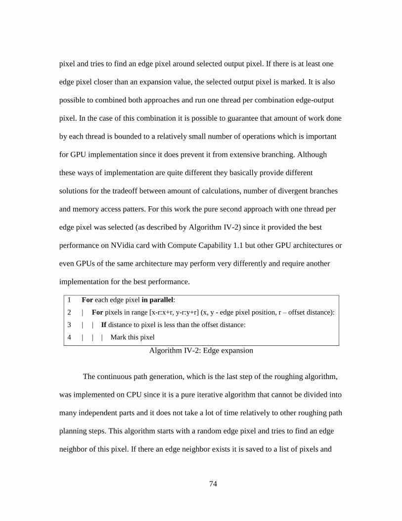
74
pixel and tries to find an edge pixel around selected output pixel. If there is at least one
edge pixel closer than an expansion value, the selected output pixel is marked. It is also
possible to combined both approaches and run one thread per combination edge-output
pixel. In the case of this combination it is possible to guarantee that amount of work done
by each thread is bounded to a relatively small number of operations which is important
for GPU implementation since it does prevent it from extensive branching. Although
these ways of implementation are quite different they basically provide different
solutions for the tradeoff between amount of calculations, number of divergent branches
and memory access patters. For this work the pure second approach with one thread per
edge pixel was selected (as described by Algorithm IV-2) since it provided the best
performance on NVidia card with Compute Capability 1.1 but other GPU architectures or
even GPUs of the same architecture may perform very differently and require another
implementation for the best performance.
1 For each edge pixel in parallel:
2 | For pixels in range [x-r:x+r, y-r:y+r] (x, y - edge pixel position, r – offset distance):
3 | | If distance to pixel is less than the offset distance:
4 | | | Mark this pixel
Algorithm IV-2: Edge expansion
The continuous path generation, which is the last step of the roughing algorithm,
was implemented on CPU since it is a pure iterative algorithm that cannot be divided into
many independent parts and it does not take a lot of time relatively to other roughing path
planning steps. This algorithm starts with a random edge pixel and tries to find an edge
neighbor of this pixel. If there an edge neighbor exists it is saved to a list of pixels and

75
become a new selected pixel. This process continues iteratively while it is possible to
select a neighbor edge pixel. At the end it starts with another random edge pixel and
performs the same process until all edge pixels are processed. Since it is not known if a
randomly selected pixel is on the end of a continuous path, when the algorithm cannot
find a neighbor near the current pixel it tries to find one near the beginning of a current
segment and connect both segments correctly. Steps performed during the continuous
path construction are shown by Algorithm IV-3
1 While there are non-processed edge pixels:
2 | Create a new path list
3 | Select a random edge pixel
4 | While there are non-processed neighbors:
5 | | Select a random neighbor
6 | | Mark selected pixel as processed
7 | | Save selected pixel to a list
8 | If initially selected pixel was in the middle of a path:
9 | | Repeat steps 4-7 for another part of a path and place results in the same list
Algorithm IV-3: Continuous path construction
The next part will explain a possible optimization technique for connecting
multiple path components into one continuous tool path with relatively short movements
between different path segments.
Tree based algorithm for path components connection optimization
One of the most important parameters of the roughing tool path planning
algorithm is the milling time. It contains time of material removing and moving of cutter

76
from one position to another. Since the material removal rate is usually a constant value it
is easy to see why the best path requires continuous material removing all the time
without cutter movement between different areas.
A machine removes material layer by layering in different areas with the
described roughing path planning algorithm, as result roughing path contains a lot of path
components for each layer and machine needs to move cutter from one area to another if
they are not connected together. This movement between different areas of each layer
costs extra milling time and may become a significant part of entire roughing time for
some specific part geometries. One of solutions for this problem is optimization of order
of sub paths while generating a roughing path automatically. There are many ways to
connect paths generated after the processing of each layer. The simplest way is to connect
all path components for each layer and process all layers sequentially. This way is easy to
implement and it works quite well in modern software but if a part contains some deep
holes machine has to move cutter from one whole to another. Figure IV-4 and Figure
IV-5 illustrate this situation. Movement from area A to area B requires to move the tool
up and down 5 times. The same situation exists with area C. As a result processing of
such part layer by layer requires too many useless motions.
Figure IV-4: Slicing test part

77
Figure IV-5: Not optimized tool path
The developed approach allows solving this problem. It is based on the fact that it
is not possible to remove more material on each layer before removing material on
previous layer, or it is not possible to remove material from any point of any layer
without removing of materials on top of this point from a previous layers (this algorithm
does not work with some special cutter which allow to do it with some limitation). It is
possible to say that each layer is a sub-layer of previous layer and it is possible to
construct a tree of layers (Figure IV-6).
Figure IV-6: Generated tree

78
A standard tree processing algorithm may be used for generating a sequence of
sub-paths. The algorithm starts with an area at the top level and checks all sub-areas on
the next layer, than it does the same operation recursively for each sub-area. When an
area does not have any sub-areas algorithm generates a roughing path for it and connect it
to a path of previous sub area. It generates the best path by processing layers and
minimizing useless movements because this path takes only one movement for moving
tool from one area to another (Figure IV-7).
Figure IV-7: Optimized tool path
This algorithm (Algorithm IV-4) can be used for optimization of paths for 3-axis
machine as well as for lathe machine and even for some specific 5-axis machine paths if
it is possible to represent them as a tree. It is also possible to optimize result path with
selecting the best order of area processing. In this case a set of classic Traveling salesman
[60, 61] problems for the distances between areas for each section has to be solved. The
solution of them will give the shortest path between different areas and minimum
roughing time as result.

79
1 For each layer:
2 | Find all independent regions
3 | For each region:
4 | | Create a tree node associated with this region
5 For each layer from bottom to top:
6 | For each region:
7 | | For each region of previous layer:
8 | | | If current layer region has common pixels with previous layer region:
9 | | | | Add an edge between their nodes
10 Use depth-first tree traversal algorithm for generating a sequence of regions
11 For each region in sequence:
12 | Generate roughing tool path
Algorithm IV-4: Tree optimization
The algorithm was tested on a real machine and in the simulator (Figure IV-8),
which was described in the previous chapter. It can be seen that it allows processing each
area separately and saves time for movement from one area to another, since it processes
every region completely before going to a next one.
Figure IV-8: Tree optimization testing result

80
GPU accelerated shifted zigzag finishing path planning algorithm
Previous parts have described the parallel implementation of the contour offset
roughing path planning algorithm and the tree based approach for optimization of path
components connection. Although in real-world scenarios the next milling step is often a
semi-finishing operation, it is not too different from roughing from an algorithmic and
parallel processing point of view. Since this research is not interested in semi-finishing,
this part goes directly to the finishing operation and its implementation.
In this work the tool offset finishing generation algorithm with a zigzag topology
tool path was selected for researching of GPU implementation. The main idea of this
approach is to separate 2d tool path topology and actual tool position calculation into two
independent problems. Generation of a 2d tool path is not computationally complex
problem and it may be done quite fast on traditional CPU. As a result 2d tool path
generation is not particularly interesting for this research and a simple zigzag tool path
generated on CPU is used for finishing tool path generation. On the other side,
calculation of an actual tool position in 3d space, which can be reformulated as
calculation of a tool height or Z coordinate since 2d position is known, is much more
complicated computational problem which requires a lot of resources. The idea of the
tool offset approach is to start with a known 2d tool position and a random tool height at
which tool may intersect a surface or does not touch it at all and find an offset required
for moving a tool at a position when it exactly touches a surface as it is shown on Figure
IV-9.

81
Figure IV-9: Tool offset
It is easy to see that the offset distance is equal to maximum vertical distance
between a target surface and a tool surface. At the same time the distance between
surfaces at every point can be expressed as a difference between height values of these
points as shown on Figure IV-10. Considering usage of the height map geometry
representation described earlier a tool offset value for each 2d tool position can be
expressed as:
(IV-1)
Where is a number of height map test points is, is a height value of a target
surface and is a height value of a tool surface.
?

82
Figure IV-10: Distance between tool and target surfaces
In order to generate a finishing tool path for an entire surface tool offset, distances
have to be calculated for every point of an initial 2d tool path.
Figure IV-11: Required testing points.
As Figure IV-11 shows, it requires testing every tool surface point for every path
point which results in many billions of test points. Considering the fact that all path point
Ti
Hi

83
offsets are completely independent and the offset calculation algorithm is very simple,
from the mathematical point of view this problem is a perfect fit for parallelization and
GPGPU implementation.
In this work the described algorithm was implemented on GPU with C++,
OpenCL and OpenGL. The OpenGL is used during the first step for a very fast
construction of a height map from an input STL model by rendering a triangular mesh
with orthogonal projection and extracting Z-buffer values which represent a height map
(Figure IV-12).
Figure IV-12: Height map generation with zigzag 2d path
On the second step, C++ code is used for generation of a 2d zigzag tool path and
OpenCL is finally used for generation tool offsets for every 2d tool path point. The
implemented version of the OpenCL code utilized independency of multiple path points
from each other for parallelizing algorithm execution. Each OpenCL thread selects a 2d
path point and processes all cutter surface points by calculating a maximum difference
between a target surface and a tool surface. The result is saved to a global memory

84
without additional synchronization since all dependent calculation happens in one thread.
The complete finishing tool path planning algorithm is shown by Algorithm IV-5.
1 Generate 2D zigzag path with zero tool height (Z coordinate) at each point
2 For each 2D path point in parallel:
3 | Initialize the tool offset value with some a large negative value
4 | For each tool surface point:
5 | | Calculate a difference between tool and target surfaces point heights
6 | | If the difference is greater than the stored tool offset value:
7 | | | Replace the offset value by the calculated difference
8 | Use the maximum difference as a new tool height value
Algorithm IV-5: Finishing path planning
Since CNC machines require control by G-code commands there was also
developed a simple post-processor that converts a sequence of tool center coordinates
into a list of G-code commands accepted by the used Okuma machine and also performs
some optimizations of a sequence like the detection of straight lines represented by
multiple points and replacing it with a single command in order to reduce an output file
size.
Experimental 3-axis path planning and milling results
During the research project, developed path planning algorithms were
implemented by using C++, OpenCL and OpenGL with support of GPU acceleration and
performed on Dell Precision M6500 mobile workstation (GPU: NVidia Quadro
FX2800M with 96 CUDA cores @1.5GHz, CPU: Intel i7-820QM, 4 cores @1.73GHz).
Implemented algorithms were used for generation tool paths and G-code programs that

85
were tested by performing both simulation in developed simulator and milling on the
Okuma MB-46VE CNC milling machine. A set of randomly selected complex 3d models
in STL format available on the Internet was used as the input for path planning
algorithms. In this part of the research, project collisions between tool holder, machine
components and workpiece were not considered and manually avoided by selecting
proper tooling and fixtures (collision avoidance will be described in following chapters
during a discussion about 5-axis orientation selection). All milling experiments used 1/8”
flat-end cutting tool for roughing and 1/16” ball-end cutting tool for finishing and were
performed with two different types of plastic. Figures on pages 85-87 demonstrate both
the simulation and milling results of the performed experiments.
Figure IV-13: Experimental milling results for the “Tiger paw” model

86
Figure IV-14: Experimental milling results for the “Sculptures” model
Figure IV-15: Experimental milling results for the “Yoda” model

87
Figure IV-16: Experimental milling results for the “Zoo” model
Discussion
In this part of the work, a set of popular algorithms were redesigned in order to
implement them on GPU and demonstrate a possibility of using GPU for tool path
planning calculations. The experimental simulation and milling results show that the tool
trajectories generated by GPU are valid and can be used for actual milling. At the same
time GPU implementation of path planning algorithms show that traditional approaches
for representing and processing geometry may be not the best choice for GPU and there
is a need for replacing them by other GPU-friendly geometry representations and
algorithms.

88
It is important to notice that the height map data structure used allows path
planning for 3-axis machines with some limitations only. There are known techniques
that allow using multiple height maps for 3+2-axis milling but there is no way to do more
general 5-axis path planning without significant changes to a geometry representation and
algorithms. Although a height map is not suitable for 5-axis milling, it is one of the best
candidates for geometry representation that can be easily processed in parallel, and it may
make sense combining more complicated data structures for 5-axis milling with some
special cases like pocket milling or initial roughing operations processed with a height
map.

89
V. 5-AXIS MACHINING SIMULATION
5-axis CNC milling is not as popular today as the 3-axis milling mainly due to its
complexity. Two additional degrees of freedom make the tool path planning process
much more complicated. They also significantly increase a chance of a collision in case
of a path planning error. And from the mechanical point of view it is much harder to
make 5-axis machines as rigid as their 3-axis analogs. Although two additional axes bring
a lot of problems and complexity, they also bring a lot of freedom and possibilities. For
example, the 5-axis milling may significantly decrease a number of setups and related
positioning errors. And what is most important is that 5-axis milling can significantly
decrease the milling time and produce better surface quality by using a more efficient tool
orientation and a shorter tool path. But in order to use benefits of the 5-axis CNC milling
the tool path planning process has to be automated or at least significantly simplified.
This chapter discusses one of the most important parts of the tool path planning
process – the milling simulation. The milling simulation is used for two different areas.
From one side it is an important component of a tool path planning process since
continuous simulation allows selection of a safe tool orientation and save time by
processing only areas that contains material. From the other side, the simulation process
is extremely important for verification of a generated tool path in safe virtual
environment before using it on a real machine.
The problem with 5-axis simulation is its complexity from the mathematical and
the computational points of view. As it was showed in previous chapters the
90
computational problem can be solved by using GPUs for calculations. But in the case of
the 5-axis simulation there are no known highly parallel algorithms and data structure
that can be used in GPGPU approach. The 5-axis workpiece cannot be naturally
represented by a height map as it was done in the 3-axis milling and there are no known
geometry representations that can be efficiently edited in parallel on GPUs, provide good
performance and memory usage. As a result there is a need for a specially designed data
structure and highly parallel simulation algorithms especially designed for 5-axis milling
simulation.
During this research project, a new volume representation was developed as well
as a set of algorithms for the 5-axis CNC milling simulation that can run on multi-GPU
systems. Although the described system is designed for 5-axis CNC milling, it is quite
general and can also be used for simulation of multi-axis machines with more than 5
axes.
This chapter describes the developed volume representation, the used data
structure, rationale behind its design and discusses its properties. It also provides
information about developed highly parallel algorithms used for rendering and editing
and the algorithms performance evaluation. Finally it describes experimental simulation
results and discusses the efficiency of the performance scalability on multiple GPUs.
Geometry representations and data structures evaluation
As was mentioned in one of previous chapters, selection of a right geometry
representation and an underlying data structure is a key component of a geometry

91
processing system. In the case of the 5-axis milling simulation workpiece geometry is not
limited as much as in the 3-axis milling and the height map representation used earlier in
this work does not fit naturally for the new purpose. It means that a new geometry
representation has to be selected or specially designed for this work.
Before going into discussion about possible solutions it is important to define a
set of features and properties that a new geometry representation has to provide.
First of all it has to be able to represent any possible geometry with high
precision and without topological limitations by using a reasonable
amount of memory.
From the parallel processing point of view, an underlying data structure
has to provide an ability to render and edit geometry in parallel with a high
level of parallelism without significant synchronization overhead.
From a scalability point of view it is important to be able to split a model
between multiple devices with very limited communication channels.
It is important to note that scalability and parallel processing are more important
than performance of serial algorithms for processing this data structure since. In contrast
to CPU, GPU performance grows over time and not limited too much by physical
limitations. So it is much easier to increase the available performance linearly just by
using more GPUs or using newer processors if a geometry representation can be scaled
efficiently. Now, existing geometry representations can be evaluated based on the
formulated requirement.

92
The most popular in the CAD/CAM field, BREP geometry representation
obviously meets the accuracy and memory usage criteria but fails both parallelization and
scalability requirements. The problem with parallelization and especially GPGPU
processing of BREP is related to the mathematical complexity of the surface elements
representation and an absence of spatial boundaries of surfaces elements. For example,
there are no boundaries on a number of surfaces that represent a given workpiece surface
region. A region can be represented either by a single surface or by a thousand of
surfaces. It means that there is no way to guarantee a high number of elements that can be
processed independently in parallel and provide enough GPU load. Possible differences
in a mathematical description of surface elements make the situation even worse since
even independent surface elements cannot be processed by the same algorithms. It results
in inefficient GPU utilization since multiple threads in the same warp have to wait for
each other and cannot process elements concurrently.
The triangular mesh represents the tradeoff between the geometry accuracy and
the surface representation complexity. It can be viewed as the BREP with surface
elements simplified to planes connected to exactly three neighbors (triangles). Using
triangles allows using the same algorithm for processing all surface elements. It results in
much more efficient geometry processing on GPU, especially in the mesh rendering
process, but it does not help with the geometry editing issues that the BREP has. In
addition the approximation of a surface by triangles requires extremely large amount of
memory for achieving high precision.

93
In contrast to boundary geometry representations like BREP and triangular mesh,
the volumetric geometry representations have a completely different set of tradeoffs.
Probably one of the simplest volume representations is the voxel model. Voxel model
subdivides an entire volume into a 3-dimensional grid of independent elements called
voxels. Each voxel has a value that may represent some properties of that area of volume
such as distance to the closest surface, amount of material or simply a presence of
material. The most important voxels property from the GPGPU point of view is their
independence. It means that each voxel can be processed completely independent from
other voxels and it can be done in parallel on multiple devices. Another important
property of the traditional voxel model is the fact that a volume is sampled regularly. It
means that there is a constant predefined number of voxels for a given volume and a
given resolution. And it results in a very simple memory management. Although the
voxel model looks like a perfect choice for GPGPU computing, since it has both
parallelizability and scalability, it has an extremely important drawback. An amount of
memory required for storing the voxel model is proportional to a third power of the
model resolution. It makes completely unfeasible using it for precision tool path planning
without additional algorithms that can overcome this limitation. For example, a 500mm
cube represented with 2micron resolution as a voxel model will require ~14PetaByte of
space for storage. This is approximately the same as an entire Google or AT&T process
every day and it is definitely not feasibly for CAM applications.
In contrast to the regularly sampled voxel model, that provides perfect
parallelizability and scalability, there is a class of irregular sampling volume

94
representation approaches. Usually irregularly sampled approaches are represented by
trees such as the octree with constant cells ratio or the k-d tree with a variable cells ratio.
Irregularly sample models provide a tradeoff between memory requirements,
parallelizability and complexity of a memory management process. They need much less
memory than the traditional voxel model, but a tree processing is usually implemented by
recursion algorithms which are not well suitable for GPU processing since GPU kernels
cannot launch other kernels (this feature is not available in GPUs currently available on
the market at least). Tree processing on GPU is a tradeoff between the number of kernel
launches (which is equal to a tree height) and the overhead required for launching each
kernel and work planning. On one hand higher (or deeper) trees provide better resources
usage and may provide higher accuracy and on another hand every additional level
requires another kernel launch and jobs planning time. An additional problem of all tree
based algorithms is the memory management. In the case of CPU processing, there is
virtually no significant memory allocation or releasing penalty, and every thread can
manage its memory independently. But there is no such natural mechanism for GPU and
the implementation of a memory management system can significantly increase an
algorithm complexity, and add extra performance penalties. Although irregularly sampled
volume representations have significant drawbacks related to GPU computing, and their
implementation itself is not trivial, it is important to note that they still provide a high
level of parallelizability and scalability. It means that an irregularly sampled volume
represented by a tree can be a good starting point for designing a data structure for

95
GPGPU accelerated simulation and tool path planning but there are additional changes
required since available implementations cannot be efficiently ported to GPU.
Approach Z-map BREP Trian.
mesh
Voxel Octree
General Bad Good Good Good Good
Accuracy Average Good Average Bad Average
Memory Average Good Average Bad Average
Rendering Average Average Good Average Average
Editing Good Bad Bad Good Average
Scalability Good Bad Bad Good Average
Complex Good Bad Good Good Average
Table V-1: Geometry representations comparison
Developed irregularly sampled volume representation
As was mentioned above, existing geometry representation approaches provide a
wide range of tradeoffs between accuracy, memory usage, parallelizability and scalability
but do not offer a perfect choice for GPU-computing. As results it is possible to note that
there is a need for a specially designed geometry representation and a corresponding data
structure that can be used for the 5-axis CNC milling simulation and tool the tool path
planning process.
Based on the geometry representations evaluation it is easy to see that volumetric
approaches are better suited for parallel processing than surface based approaches, mainly
because of independence of volume elements which can be processed independently and
predictability of a workload. It is also more natural for the milling simulation to represent

96
a volume since the actual physical process is the volume removing process. It is also
obvious that the regularly sampled volumetric approach (such as the voxel model) cannot
be used due to memory requirement, and that there is a need for an irregularly sampled
representation. However even irregularly sampled tree-based representations cannot
achieve a BREP level of accuracy with reasonable memory requirements. For example,
considering the representation of a 500mm cube with 2 micron elements (as an example
of a work area and accuracy found in modern 5-axis machines) and 1 byte per element, a
simple part would require ~350Tb (6 sides * (500 mm /side / 0.002 mm)^2) of data just
for surface representation without considering a data structure overhead. It is much more
than modern personal computers can store and process in a reasonable time. It also means
that the available volumetric geometry representations will always have a limited
precision in comparison to the actual machine precision. From one side it may look like it
is a fundamental limitation that cannot be overcome. But from another side there are not
so many use cases with a real need of the extremely high accuracy. It may be more
efficient to use data structures with lower accuracy and some workarounds for these
special cases.
After accepting the fact of accuracy limitation for volumetric data representations,
the next step is to make a decision about the tradeoff between memory usage, accuracy
and parallelizability. There are two main relations between these parameters. First, more
complicated data structures provide higher accuracy for a given amount of memory.
Second, deeper trees provide more efficient memory usage for a given accuracy.
Relatively complicated data structure with non-predictable density such as k-d trees are

97
less suitable for this research due to GPGPU specific load balancing (the problem similar
to the BREP) and editing problems. Although generally they provide higher efficiency,
their processing algorithms are more complicated, often have non-linear memory access
patters and have a higher branch divergence. These properties result in significant
performance penalties on modern GPUs. As a result, it is possible to note that considering
the existing GPU architectures the designed data structure has to be as simple as possible.
One of the simplest possible tree-based volumetric representations is a tree with nodes
where each node represents a regularly sampled volume and a list of references to its
children. The octree is a classic example of this type of geometry representations with 8
children per node.
One of the most important steps is the selection of a number of children and
amount of geometrical data stored in each tree node. It is easy to see that a higher
children number reduces memory usage efficiency (in an extreme case a tree becomes a
voxel model) and a tree depth for a given accuracy. But it is also important that a
geometry processing can be efficiently parallelized by processing each child of a node
concurrently. If this is done by a warp, it makes memory access more efficient by storing
children data in a continuous memory block which can be read linearly in one memory
access operation. Considering the amount of geometrical data stored in a node it is
possible to say that more data approximates geometry better but uses more memory. On
one side of this tradeoff, each node contains a complete mathematical description of all
geometry elements. And on the other side, it is possible to use only one bit to store
information about presence of material in a nodes volume (or store a byte that describes a

98
distance to a surface or material density as it is done in the traditional voxel model). The
first approach is similar to the BREP and has similar problems. Complete geometry
description requires using complex algorithms and complicated memory management
since it is not possible to predict a content of a node after editing. The opposite approach
is actually much more GPU-friendly because the amount of data is constant, geometry
processing algorithm is much simpler and all nodes use exactly the same geometry
processing algorithm.
Based on the described tradeoffs there was designed a volumetric data structure
for the GPGPU accelerated multi-axis CNC milling simulation and the tool path planning
(Figure V-1). The developed geometry representation is a 2-level hybrid of the tree and
the voxel model. It uses a 3d array of cells that represents a regularly sampled volume.
Each cell stores 2 bits of geometrical data (similar to voxel model) and a pointer to an
array of 4096 children (similar to a tree). Cells children (called “subcell”) represent a
regularly sampled (16x16x16) volume and store 2 bits of geometrical data but do not
store pointers to their children. 2 bits geometrical data is used for 3-color scheme for
geometry representation. They represent 3 possible states of a cell or subcell:
Cell is completely filled by material
Cell is completely empty
Cell state is unknown and it probably contains a boundary

99
Figure V-1: Developed geometry representation model
In contrast to traditional cubical voxels, cells or subcells represent spheres
circumscribed around traditional cubes calculated by volume subdivision.
The Figure V-2 demonstrates a surface representation example with the 2D
version of the described geometry representation and square cells.
Figure V-2: 2D example of the developed model surface representation
From a hierarchy point of view, it can be viewed as a 2 level tree as shown on
Figure V-3. It is important the low level nodes that represent subcells are stored in voxel
models. But information about high level nodes is stored in a list. As result, links between
Cells
Subcells
Surface
Full Boundary Empty
Voxel model
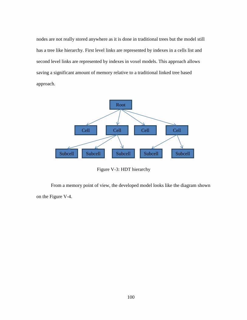
100
nodes are not really stored anywhere as it is done in traditional trees but the model still
has a tree like hierarchy. First level links are represented by indexes in a cells list and
second level links are represented by indexes in voxel models. This approach allows
saving a significant amount of memory relative to a traditional linked tree based
approach.
Figure V-3: HDT hierarchy
From a memory point of view, the developed model looks like the diagram shown
on the Figure V-4.
Root
Cell
Subcell
Cell Cell Cell
Subcell Subcell Subcell Subcell
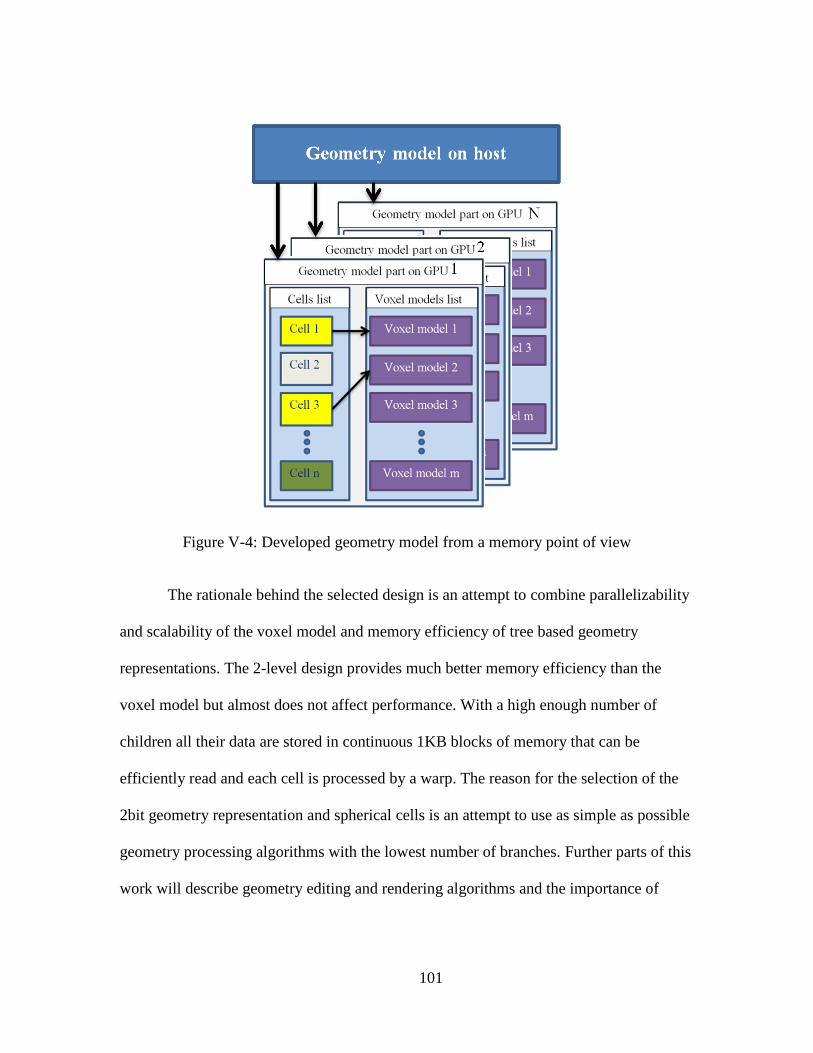
101
Figure V-4: Developed geometry model from a memory point of view
The rationale behind the selected design is an attempt to combine parallelizability
and scalability of the voxel model and memory efficiency of tree based geometry
representations. The 2-level design provides much better memory efficiency than the
voxel model but almost does not affect performance. With a high enough number of
children all their data are stored in continuous 1KB blocks of memory that can be
efficiently read and each cell is processed by a warp. The reason for the selection of the
2bit geometry representation and spherical cells is an attempt to use as simple as possible
geometry processing algorithms with the lowest number of branches. Further parts of this
work will describe geometry editing and rendering algorithms and the importance of

102
spherical cells for making them simpler. 2 bit data structure also allows increasing
resolution almost twice with the same memory usage in opposite to the traditional voxel
model (1 byte per voxel). The used design also achieves great scalability. Since all cells
are completely independent they are stored on multiple GPUs (and possibly on multiple
computers) and processed independently with the almost linear performance
improvement. The multi-GPU scalability will be also discussed later in this chapter.
Although the detailed performance evaluation will be provided later in this work,
it is important to note that the designed data structure showed great parallelizability and
scalability. The 3-GPU configuration successfully simulated and rendered in real-time a
workpiece represented with the resolution of 6000^3 which is not feasible for a
traditional voxel model due to memory usage.
Tool motion representation for 5-axis milling simulation
Before describing actual milling simulation algorithms it is important to discuss a
machine tool representation since it significantly affects material editing algorithms. One
of the most popular tool models used in researches is a generalized tool model shown on
Figure V-5 and described by Chiou and Lee [62]. It contains three main parts: lower and
upper cones and a torus component. The benefit of this model is an ability to represent a
wide range of popular cutters with the same model. For example, a ball-end mill can be
represented by completely eliminating both cones or a flat-end tool can be represented by
eliminating torus component.

103
Figure V-5: Generalized tool model [62]
At the same time this model is not the best solution for a GPU-oriented simulation
system. In order to understand why it is not the best choice it is important to look on
description of 5-axis motions of this tool. Chiou and Lee [62] provide solutions for swept
profiles of a torus (V-1) and cones parts (V-2), (V-3). It is easy to see that the depicted
solutions have many trigonometric functions. It means that actual computing kernels will
have to calculate quite many trigonometric operations which are quite slow on modern
GPUs especially if full precision is used.

104
(V-1)
(V-2)
(V-3)
Although the presented solution can be used, and it does provide the generalized
tool support, this work is oriented on a search for GPU-friendly solutions. As result, there
was selected a tool representation approach similar to the Constructive Solid Geometry.
A tool is represented as a set of simple geometry shapes such as spheres, cylinders,
planes. And a swept volume of each simple shape is also a simple shape. For example a
sphere makes a swept volume that can be described by two spheres and a cylinder. A

105
cylinder at the same time makes a swept volume that can be described by a prism and two
cylinders.
It is important to notice an important assumption made in this work: true 5-axis
motions can be approximated accurately by a set of 3+2 axis motions. Although it is not
generally true, true 5-axis motions are not as popular as 3+2 axis motions even on 5-axis
machines. And even in case of true 5-axis motions only a tip of a tool is used most of the
time and the assumption is valid in this case. At the same time the selected approach can
be used for representing true 5-axis motions but swept volumes of simple shapes in this
case become much more complicated and they are not discussed in this work.
The selected tool representation approach has multiple benefits. First of all, very
simple geometric tests can be used for detection if a cell or subcell is completely inside or
outside of a tool swept volume. Another benefit is the even higher possible
parallelizability since different tool swept volume components can be processed
completely independently. For example, formulas (V-4), (V-5) show how a cell can be
tested.
| |
| |
[| | ] [( ) (| | )]
(V-4)

106
| |
| |
[| | ] [( ) (| | )]
(V-5)
f represents a Boolean value, which means that a cell is fully inside of a swept
volume and e represents that a cell is completely outside and not affected by this tool
movement. It is noticeable that all operations in these formulas are very simple and
actually implemented in GPU hardware. Formulas represent geometric tests for a steady
tool. Although, in case of actual movements, these formulas will get additional
components and become a bit more complicated. . As it is shown on Figure V-6 a 3+2
axis tool movement will create an additional prism and cylinder. All geometric tests for
these shapes will still be efficient since almost all of them are based on hardware
implemented vector operations.
Figure V-6: Ball-end tool swept volume model
P
N
0 R

107
5-axis milling simulation based on irregularly sampled volume
The previous part describes the selected tool representation and the reasons why it
is better to use a CSG based tool model than a traditional generalized cutter
representation. This part goes forward and discusses implementation of the developed
geometry representation and the material removing simulation algorithm. It is based on
the assumption that there are known solutions for determining if a spherical cell is
completely inside, outside or on the boundary of a tool swept volume one of which is
shown in the previous part.
The implementation of the developed geometry representation model (called
Hybrid Dynamic Tree or HDT) contains 3 main parts: array of cells, pool of subcells and
a memory map. In contrast to a traditional voxel model, which stores all cells information
in a 3d array, the HDT uses a constant length list (implemented as 1d array) where every
element contains coordinates of a cell, cell value and a reference to a subcells node. The
rationale behind this way of storing data is improving of the data structure scalability.
During a data structure initialization time an entire space that has to be represented is
regularly subdivided into cells as it is done in a voxel model. Then, based on the number
of computing devices (in the current implementation, GPUs), each cell is randomly
mapped to a specific device and the generated map is stored for using during initialization
of other data structures on the same computer. Random mapping with uniform
distribution guaranties that every device gets a reasonable equal amount of work (cells to
process) for any possible spatial distribution of edited cells. This fact is a key component
for the efficient load balancing of multi-GPU configurations. The developed

108
implementation actually divides cells based on an estimation of a device performance for
improving load balancing of systems that have multiple different GPUs as it is shown on
Figure V-7.
Figure V-7: Multi GPU load balancing
Every cell contains the complete information required for cell editing or rendering
and can be processed completely independent from other cells. It is required for better
scalability since each computing device needs to store only a subset of all cells and does
not need information from other cells. It significantly reduces traffic between host and
GPUs since each GPU has all required information in its own memory.
During a milling simulation the simulator processes a sequence of tool
movements. Each tool movement is represented as a set of geometric primitives and each
GPU calculates if there are cells intersecting one or more of these primitives. Generally
each GPU performs a set of geometric tests, similar to those described in the previous
part, in order to determine if a cell is intersected or hovered by a tool movement swept
volume. If a cell lies completely inside of a tool swept volume, it is marked as an empty
cell and its subcells node is released (if it was a boundary cell). If a cell is intersected by
one or more tool swept volumes it is added to a list of cells that have to be further
processed. The Algorithm V-1 demonstrates the first part of the simulation algorithm.

109
1 For all cells in parallel:
2 | For all tool motions:
3 | | Calculate intersection between cell and swept volume
4 | If cell lies inside of at least one tool swept volume:
5 | | If cell is full:
6 | | | Mark cell as empty
7 | | If cell is boundary:
8 | | | Mark cell as empty and add to a list for subcells cleaning
9 | Else:
10 | | If cell is intersected by swept volume:
11 | | | If cell is full:
12 | | | | Allocate memory for subcells from a memory pool
13 | | | If cell is not empty:
14 | | | | Add cell to a list for subcells processing
15 For all cells in cell cleaning list:
16 | Mark all subcells as full
17 | Return memory allocated for subcells to a memory pool
Algorithm V-1: First part of the machining simulation process
1 For all cells in subcells processing list in parallel (per multi-processor):
2 | For all subcells in cell in parallel (per core):
3 | | For all tool motions:
4 | | | Calculate intersection between subcell and swept volume
5 | If subcell lies inside of at least one tool swept volume:
6 | | Mark it as empty
7 | Else:
8 | | If subcell is intersected by at least one swept volume and subcell is not empty:
9 | | | Mark it as boundary
Algorithm V-2: Second part of the machining simulation process

110
The second part (shown by Algorithm V-2) of the material removing algorithm is
the processing of subcells. During processing cells each GPU generates a list of cells
intersected by a swept volume. This list is used for selecting subcells that have to be
further processed. The algorithms performs the same set of geometric tests to each
subcell and determines if a subcell is completely inside of a swept volume, completely
outside or interested. Subcells that lie completely inside of a swept volume are marked as
empty. Subcells intersected by a swept volume are marked as boundary if they were
completely full by material. The Table I-1 shows the possible cell value changes based on
results of geometric tests.
Cell \ Swept volume Inside Intersected Outside
Full Empty Boundary Full Boundary Empty Boundary Boundary Empty Empty Empty Empty
Table V-2: Cell value changes
a) Initial surface representation

111
b) Results of intersections between cells and a tool swept volume
c) Geometry model after machining simulation
Figure V-8: Machining simulation process shown on 2D geometry model
The Figure V-8 demonstrates the machining simulation process and different
states of the underlying geometry representation model. The first part “a” demonstrates
an initial state of a geometry model that represents a surface, green color represents cells
with material and yellow color represents boundary cells. The second part “b” shown a
tool swept volume (just a slice of it in case of this 2D example) and calculated
intersection results between cells and tool swept volume. Here, the orange color

112
represents the cells that lie completely inside of a swept volume. These cells will be
removed. The green color in this case represents the cells that lie completely outside of a
swept volume; they will not be affected at all. The last part “c” represents a geometry
model state after machining simulation. It is easy to see that that some cells have been
subdivided into subcells since they contain surface now and some cells which earlier
contained subcells are completely empty.
Although the subcells value updating algorithm is relatively simple and straight
forward, it is important to notice some GPU-specific implementation details. Each cell
contains an array of 16x16x16 subcells and each subcell is represented by 2 bits. The
selection of these parameters is critical since they determine both performance and
memory efficiency. In this work each block of subcells is processed by an independent
warp for decreasing data exchange between warps and eliminating additional
synchronization. It means that all of the warps in a work group are completely
independent and use internal synchronization without any memory access barriers for
improved performance. From another side each thread in a warp read a 32 bit integer that
stores a consequent block of 16 subcell values as shown on Figure V-9, processes it and
stores updated values back. It results in perfectly linear and efficient memory reading and
writing operations which are extremely important due to GPU memory controller
limitations. This is possible because all of the subcells are independent from each other
and their values can be updated in private memory of a thread that processes a subcell.
The described way of processing subcell blocks is extremely important on GPU since
GPU memory controller always operates with a relatively large block of memory (32*4b

113
for used cards). And the best memory bus usage efficiency can be achieved only if all
values are used in calculations by a warp. The same limitation also becomes a problem
for using the traditional Octree since every iteration require processing only 8 elements or
16bit of data. If the algorithm uses only 16 bit of data it means that it uses only 1.5% of
the memory bus (for used NV GTX580) which is extremely inefficient.
Figure V-9: Threads distribution during subcells editing
Another interesting implementation detail is the memory management. The
OpenCL used in this work does not allow allocating and releasing memory from the GPU
kernel code. (Actually, even traditional Windows memory system does not work
efficiently in case of continuous allocation and releasing of small blocks so the described
algorithms would be useful for CPU implementation). As a result, memory management

114
is implemented by storing a nodes pool, where each node has enough space for storing a
16x16x16 block of subcells, and an address stack (implemented as an array of nodes
indexes and an index of a top element) of available blocks. Initially, the nodes pool is full
of nodes that represent completely full subcells and the address stack stores references to
all nodes. When the algorithm finds that a completely full cell is intersected by a swept
volume and its subcells have to be further processed, it pops a top address from an
address stack and associates an empty node with this cell.
The nodes releasing algorithm is a bit more interesting and complicated. The
problem with nodes releasing is related to node values. After using a node for storing
subcells values in an edited cell, it obviously has random values. But a newly allocated
node has to be “clean” or has to have all “completely full” subcell values. The cleaning
basically means that all subcell values are changed to “completely full” state and it is
nothing more than writing some predefined values to a node memory. Although it may
look like a simple and trivial operation, the decision of when to do the cleaning is not as
trivial and significantly affects performance. There are two obvious ways to do cleaning:
during node allocation (during cell editing operation) or during node releasing. Both of
these ways have a significant problem: it is not known when they happen and they almost
always happen in few threads of a warp. It brings two important problems. First, if only
one thread in a warp needs to get or release a node, 31 other blocks have to wait until it
works with a node. Second, only one thread has to clean an entire node which means that
it has to issue 32 times more memory writing commands and use 1/32th of a memory bus
than it is really needed. As result memory management works very slowly. The

115
developed solution is using a temporary list of nodes (Figure V-10) that have to be
cleaned before returning to the nodes pool and centralizing cleaning of these nodes by all
warp threads. As was mentioned before, nodes go from the nodes pool to the geometry
model when a cell is intersected by a swept volume and there is a need to represent a cell
with higher accuracy by subdividing it into subcells. There are two possible ways for a
node to go back. First, a cell lies completely inside of a swept volume and it becomes
completely empty in result. Second, it is detected that all subcells of a cell are empty and
an entire cell can be marked as an empty cell. In both cases a node goes to a temporary
cleaning storage. When an application is idling it can run the node cleaning algorithm
that rewrites nodes values and return them back to a node pool. It may significantly
improve memory management performance and allows the use of idle time for useful
operations.
Figure V-10: Nodes memory management model
Irregularly sampled volume rendering algorithm
The geometry editing process is only part of all the geometry representation jobs.
Another important part is data visualization, or geometry rendering. The rendering
process is important from two points of view. From one side, showing geometry to a user
Nodes
pool
Node allocation
Node cleaning
Cleaning
storage Node releasing
Geometry
model

116
may be a goal of an application, for example, showing of a milling simulation result is
one of main goals of a simulator. From the other side, even if an application does not
have to produce any visual output, rendering still may be important for debugging
purpose. This part describes rendering algorithms designed especially for the developed
geometry representation and efficient highly parallel multi-GPU rendering.
As was mentioned earlier some geometry representations such the triangular mesh
or the voxel model can be rendered directly but other model such as the height map has to
be converted to another geometry representation for rendering. There are many rendering
techniques that have been developed for various situations and geometry representations.
For example, a ray tracing approach attempts to simulate a physical world and can
produce a photorealistic image. However it requires a lot of computational resources and
cannot be easily parallelized. On the opposite side, a ray casting approach can be easy
parallelized but usually produces not physically realistic images. The developed in this
work approach uses a mix of ray casting and direct rendering approaches for producing
an image that is not photo realistic but provides even more useful information than a
physically accurate pictures. The proposal for this research project contained description
of a possible rendering technology for the proposed geometry data structure. Since during
the research project there was made a decision to use the simplified version of a volume
representation, the actually implemented renderer uses a simplified algorithm adopted for
the simplified data structure. However it is important to describe the originally proposed
approach since it may be implemented in future for more complicated geometry
representation.

117
The originally proposed rendering algorithm works in two steps. First it iteratively
generates a height map oriented as a screen by casting rays from each filled cell to a
screen plane and subdividing the visible boundary cells to increase the resolution until the
size of each cell becomes smaller than half of a pixel size. Then normals are calculated
for each height map point for a correct lighting. There are two possible options for
normal calculation: the first is to estimate normals directly from a height map which will
produce reasonable results. The second option is to calculate normals based on analytical
information about a surface which has to produce exact values for normals but requires
additional calculations. In this case the algorithms will identify the closest surface that is
represented analytically and use an analytically calculated normal at the closest surface
point. The closest point is not always an actual ray intersection point; however, the
maximum possible error cannot be greater than the pixel size. Therefore, it is possible to
assume that a surface is continuous and the calculated normal approximates the actual
normal to a high degree of accuracy. Figure V-11 shows the results of the two iterations
used by rendering algorithm to generate a height map where red line shows actual surface
and yellow line shows an approximated height map value at each pixel.
Figure V-11: Two height map generation iterations used for rendering

118
The Figure V-11demonstrates only an idea of an algorithm for generating a height
map that can be used for true dynamically generated geometry models. Actually
implemented geometry model has only 2 levels and use spherical cells in opposite to
shown rectangular cells as shown on following figures that describe a rendering process.
The implemented rendering algorithm starts by creating a list of all boundary cells
that are shown on Figure V-12 in yellow.
Figure V-12: Curve represented by spherical cells
Then it processes all boundary cells and creates a list of boundary subcells as
shown on Figure V-13.

119
Figure V-13: Curve represented by spherical subcells
A list of boundary subcells is the main input for the next big step of the rendering
algorithm. It is important to notice that these cells are completely independent and may
actually be stored on different GPUs. The problem here is that multiple cells from
different devices may affect the same pixel. As result there is a need for additional
synchronization. Since synchronization reduces performance, the implemented algorithm
is trying to do as much work as possible simultaneously on multiple GPUs and then
synchronize results. One of the most important steps that it does in parallel is calculation
of a height map by calculating distances from a rendering plane to the closest cell.
However, as was mentioned above, each GPU has only part of the volume, and as a result
each GPU calculates only distances to cells that are stored on this GPU.

120
Figure V-14: Rays casted from each pixel on a screen plane
The current implementation does not actually cast rays from screen plane but
casts them from each cell to a screen plane and stores the closest distance for each pixel
as shown on Figure V-14. When all distances are calculated, they are downloaded to one
GPU and combined there into a one complete real height map (before this step, GPUs had
only parts of a height map although they were stored as a height map).
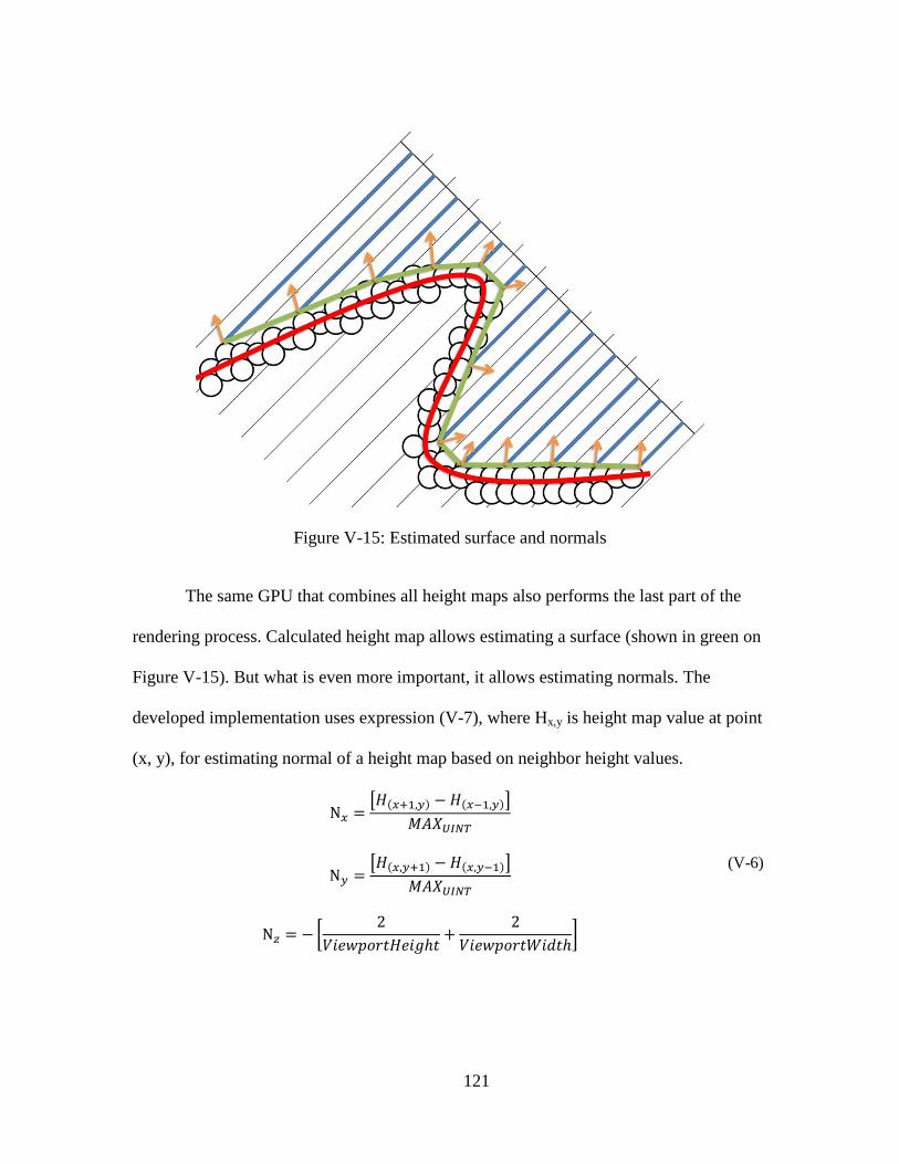
121
Figure V-15: Estimated surface and normals
The same GPU that combines all height maps also performs the last part of the
rendering process. Calculated height map allows estimating a surface (shown in green on
Figure V-15). But what is even more important, it allows estimating normals. The
developed implementation uses expression (V-7), where Hx,y is height map value at point
(x, y), for estimating normal of a height map based on neighbor height values.
[ ]
[ ]
[
]
(V-6)

122
When normals are estimated for each surface point associated with a screen pixel,
a surface intensity is calculated as a dot product of a normal vector and light direction
vector. An actual pixel value is calculated as a product of surface point intensity and a
surface material color.
The complete list of steps performed during rendering process is shown by
Algorithm V-3.
1 Collect a list of all boundary cells in parallel
2 Collect a list of all boundary subcells in parallel
3 For all subcells in parallel:
4 | Calculate cell projection to a screen plane
5 | For all pixels in projection area:
6 | | Calculate a distance between screen plane and cell surface
7 | | Update pixel value by a minimum between current value and calculated value
8 Combine height maps from multiple devices
9 For all pixels in parallel:
10 | Estimate normal values
11 | Calculate pixel color
Algorithm V-3: Rendering
The Figure V-16 demonstrates rendering results of the implemented rendering
algorithm. It is similar to the original rendering algorithm but it has one significant
limitation. It uses only single iteration, since the underlying data structure is static and
limited to 2 levels. The implemented renderer cannot show perfect accuracy due to
geometry model limitation but it already runs on 3 GPUs with almost linear performance
improvement which is a very hard task that cannot be achieved even by multi-million
computer games.

123
Figure V-16: Rendering results
It is interesting to notice that the selected method of normals reconstruction from
a height map results in interesting visual effects. If one object stays in front of another
object then it is not only rendered in foreground but there is also shown a dark border
when it intersects deeper object. Figure V-17 demonstrates this effect. It is very easy to
see which line is closer and which line is deeper.
Figure V-17: Demonstration of dark borders around foreground objects
124
Accuracy analysis
The simulation of any process does not make sense if the simulation is not
accurate enough. The key word in the previous sentence is “enough”, but there is no
information about desired accuracy. It is obvious that perfect sub-atomic level simulation
would be nice to have but would it really help in a machine shop from a practical point of
view? It can be seen that sub-atomic level simulation would be quite slow. It would
probably be at least a thousand times slower that actual machining and this level of
performance already makes it useless. What is more interesting is that it is actually
impossible to achieve sub-atomic precision level just because modern CNC machines
cannot achieve this level of accuracy. Before discussing the accuracy of the developed
simulator it is important to understand possible precision limits and practical
requirements for machining simulation from an end user point of view.
Modern CNC controllers limit the input tool path accuracy to 0.002mm. It means
that it does not make sense to simulate anything with input trajectory accuracy higher
than 2µm because a machine does not know about this extra precision in any case. But
2µm is pure software limit that is not connected to physical world. During the machining
process, the accuracy is affected by tool vibrations, external vibrations, thermal
expansion, material deflection, etc. And many of these parameters cannot be measured
because they depend on environment condition, tool properties, workpiece properties, etc.
As result, 2µm precision can be achieved only in very well controller environment on
expensive machines, tools and after good preparation. Most of real life machining
provides more than an order of magnitude lower accuracy (20-50µm) that is still good

125
enough for most practical applications. It is easy to see that in most cases, simulation
with precision higher than 20-50µm (2µm in very special cases) does not make sense at
all since the actual accuracy is limited by machine capabilities.
Limits described in the previous paragraph are based on the machines limitations.
This paragraph will discuss what makes sense from the end user point of view. But before
going into this discussion it is important to describe use cases for machining simulation
software. Most popular use cases include: collision detection, exceeding axis movement
limits, exceeding tool load limits, overcuts detection and surface quality control. The
collision detection has two components: collisions of machine parts (including tool and
tool holder) with each other that and collisions between machine parts and workpiece.
Collision detection between machine parts and exceeding axis limits actually do not
require material removing simulation and are not discussed here. Now, when most
popular use cases are listed, their simulation accuracy requirements can be discussed.
The collision detection process need to know if a machine part intersects
workpiece material. Since it is not safe to have moving machine parts closer than few
millimeters to material surface (for parts under 500mm long), it is safe to assume that
0.5mm accuracy of surface position is good enough for the collision detection purpose.
Overcuts detection is a bit more complicated problem. It can be viewed as collision
detection between tool and target geometry in case of large overcuts and it can be viewed
as a bad finishing surface quality in case of small overcuts. For large overcuts scenario
the same requirements as for collision detection can be used and it is safe to assume that
0.5mm accuracy is enough. Small overcuts and finishing surface quality control are two

126
most demanding use cases. Their requirements depend on the desired surface tolerance
and generally it is possible to say that it is does not matter where surface is as far as it is
possible to prove that it lies in tolerance limit. As an example of possible tolerance limits
let use the ANSI B4.1 standard [63]. Figure V-18 shows tolerance limits for multiple
grades defined in this standard. The milling process under normal conditions is capable of
producing parts with tolerance grade in the range 10-13. For example, considering the
best possible grade and a part with a size of 50mm the tolerance limit defined by the
standard is ~0.1mm. And for a 500mm part which is a quite popular work envelope limit
for modern 5-axis CNC milling machines, the tolerance limit is ~0.25mm.
Figure V-18: Tolerances for multiple tolerance grades [64].
Now, when there are known accuracy requirements for popular milling simulation
usage scenarios, it is possible to discuss capabilities of the developed simulation system
and to see if it meets the requirements. The developed geometry representation does not
127
naturally represent surface but stores information about presence of a surface in each cell.
As a result, surface position can be measured with precision limited to a small cells size
and it is possible to say that geometry representation accuracy is equal to a size of the
smallest cell. It is also important to mention that due to using spherical cells, linear cells
size has to be multiplied by ~1.732. Considering resolution of 4096x4096x4096 for a
workpiece with dimensions 50x50x50mm, it is easy to see that a cell size is ~0.021mm.
For a larger workpiece (500x500x500mm) the resolution will be ~0.21mm.
It is easy to see that simulation with a resolution of 4096x4096x4096 meets
requirements for all popular machining simulation use cases for parts with dimensions up
to 500x500x500mm which is a common machining envelop size for modern 5-axis
machines and the most accurate tolerance requirements for the ANSI B4.1 standard. It is
also easy to see that for smaller parts such as 50x50x50mm a resolution can be reduced
by 2 or even 4 times without significant problems from practical point of view.
Performance benefits of resolution reduction will be described later. Although the
developed system meets the precision requirements for popular use cases, its precision is
quite close to this requirements and it is important to notice that it cannot be used for
extra high precision simulation without modifications. In case of a need for highly
accurate simulation, a possible way to do it is to implement the full version of the initially
proposed geometry representation that can be dynamically generated. But as was
mentioned earlier, even the already developed system is accurate enough.

128
Experimental 5-axis simulation results
The described data structure and algorithms were implemented during the
research project. All low level highly parallel algorithms and data structures were
implemented in C++ and OpenCL. High level algorithms and data management were
implemented in Python. And a rendering was implemented as a mix of OpenGL with
OpenCL based custom software renderer running on GPU. The developed system
successfully uses a multiple GPUs (tested with 2 x GTX 580 + Quadro 6000) and
provided good performance and scalability results which will be discussed later.
The set of input G-code files used for testing contains mainly programs generated
by tool path planning solutions discussed in this work (both 3 and 5 axis) as well as few
test programs from industrial partners.
The first part of the testing process is simulation of previously described 3-axis
parts from chapter about 3-axis machining simulation and tool path planning.

129
Figure V-19: 3-axis model “Sculptures” (new 5-axis simulator on the right)

130
Figure V-20: 3-axis model “Zoo” (new 5-axis simulator on the right)
Figure V-19 and Figure V-20 demonstrate the results of the developed 5-axis
simulator in comparison to the height map based 3-axis simulator from previous chapters.
It is easy to notice that the produced results are very similar to the original 3-axis
simulation results except color (easy adjustable) and projection type. The original 3-axis
simulator uses perspective projection and the new 5-axis simulator uses orthogonal
projection.

131
The next part of the testing process is the continuous simulation of 5-axis parts.
Since an editing process is a continuous test pictures will demonstrate workpiece state at
multiple time points during an editing process with a target geometry model at first image
and actually milled part on the last image.
Figure V-21: 5-axis machining simulation process for model “Puppy”

132
Figure V-22: 5-axis machining simulation process for model “Fan”

133
Figure V-23: 5-axis machining simulation process for model “Fan”
Figure V-24: Simulation result for model “Dragon”

134
Figure V-25: Roughing process of the “Teapot” model
Figure V-26: Various simulation results
Figures above demonstrate that the developed 5-axis simulation system is capable
producing accurate CNC milling simulation by using the newly developed geometry
representation and parallel algorithms that can run on multiple GPUs. It is also easy to
see the high quality of images produced by implemented rendering algorithms. The
comparison of the simulator output to real machined parts also shows that simulated
results accurately predict machined results.

135
Simulation performance analysis
The previous part demonstrated that the developed 5-axis simulator is capable of
producing correct simulation results. This section will discuss performance measurements
of the simulation and rendering algorithms as well as scalability issues.
First of all it is important to describe how performance will be measured since
there are no known tests for CNC machining simulators at time of testing and by the
author knowledge. Since there is no significant dependency between target shape and
underlying algorithms behavior, material removing test is designed to be as simple and as
general as possible. It simulates removing a layer of material from a cube workpiece as
shown on Figure V-27. The rendering test will actually use the result of the material
removing test and render the machined workpiece from multiple sides.
Figure V-27: Machining test setup

136
All performance measurements are performed with following default parameters:
Resolution of 2048x2048x2048. For simplicity only one number will be
written latter but it is always a cube of a material;
A big cell contains 16x16x16 small cells.
Step size is 64. The step size is a number of tool movements processed
concurrently during each material removing simulation operation;
Zoom level is 1X (as shown on Figure V-27);
The test computing system includes 3 NVidia GPUs (Table V-3):
o 2x GeForce GTX580
o 1x Quadro 6000
Name CUDA cores Clock frequency IPC SP GLOPS
GeForce GTX580 512 1594 MHz 2 1632
Quadro 6000 448 1147 MHz 2 1027
Table V-3: GPUs parameters
The default configuration demonstrates performance results shown in Table V-4.
Simulation speed (mm/min, ms/mm) 24414, 0.04
Simulation speed (edits/s, ms/edit) 897, 1.11
Rendering speed (ms, fps) 60, 16.5
Table V-4: Base performance results
The difference between the two ways of measuring simulation speed is related to
the fact that tool motions may have different length and as result remove significantly
different amount of material. The first row represents the simulation speed measurement

137
technique normalized from distance point of view. Basically it shows how long trajectory
can be simulated in a minute or how many milliseconds required for simulation of one
millimeter of a tool path. Using mm/min units also allow direct comparison to a machine
feed rate. For example simulation speed of ~25000 mm/min means that simulation can be
done 5X times faster than machining at feed rate of 5000 mm/min. Another measurement
way uses the actual number of tool movements called “edits” and useful in case when
there are many short tool movements. The idea behind these performance measurement
techniques is similar to measurement storage performance that can be done from
bandwidth point of view or from number of input/output operations point of view.
It is also important to notice that the developed simulation is not a production
grade software system that is precisely tuned and optimized. As result it is more
important to measure not a pure simulation performance itself (although it is good
enough even now) but how well it scales with respect to available computational
performance, resolution, etc. Although the performance of current implementation can be
significantly improved by optimization for desired hardware, scalability and
parallelizability cannot be improved so easily, and they were the initial goal for the new
geometry representation and algorithms design.
One of the most important properties of any simulator is accuracy. As was
mentioned above, the data structure implemented in this work is static and as a result,
accuracy is directly related to model resolution. At the same time resolution obviously
affects a number of elements that have to be processed for editing simulation. In case of
pure 3D discrete volume representation such as voxel model, the number of elements is
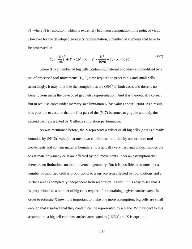
138
N3 where N is resolution, which is extremely bad from computation time point of view.
However for the developed geometry representation, a number of elements that have to
be processed is:
(
)
(V-7)
where X is a number of big cells containing material boundary and modified by a
set of processed tool movements. T1, T2 time required to process big and small cells
accordingly. It may look like the complexities are O(N3) in both cases and there is no
benefit from using the developed geometry representation. And it is theoretically correct
but in real use cases under memory size limitation N has values about ~2000. As a result,
it is possible to assume that the first part of the (V-7) becomes negligible and only the
second part represented by X affects simulation performance.
As was mentioned before, the X represents a subset of all big cells (so it is already
bounded by (N/16)3 value) that meat two conditions: modified by one or more tool
movements and contain material boundary. It is actually very hard and almost impossible
to estimate how many cells are affected by tool movements under an assumption that
there are no limitations on tool movement geometry. But it is possible to assume that a
number of modified cells is proportional to a surface area affected by tool motions and a
surface area is completely independent from resolution. As result it is easy to see that X
is proportional to a number of big cells required for containing a given surface area. In
order to estimate X now, it is important to make one more assumption: big cells are small
enough that a surface that they contain can be represented by a plane. With respect to this
assumption, a big cell contains surface area equal to (16/N)2 and X is equal to:

139
(
)
(V-8)
Where, S is modified surface area. Now the (V-7) can be rewritten in the form:
(V-9)
Based on (V-9) it is possible to assume that at reasonably low values of N (such
as few thousands) the machining simulation algorithm should show a quadratic
dependency of simulation time and resolution. The experimental performance
measurement shown on Figure V-28 has proved the assumption about quadratic
simulation complexity. It is easy to see that the 2nd
order approximation of processing
time data perfectly describes measured results.
Figure V-28: Editing time vs. Resolution
As was shown above, the newly developed geometry representation has managed
to reduce machining simulation complexity from cubic to quadratic. But this is only one
of the important benefits that the new data model provides. Other extremely important
0
0.02
0.04
0.06
0.08
0.1
0.12
0.14
0.16
0.18
0.2
0 1000 2000 3000 4000 5000
Pro
cess
ing
tim
e, m
s/m
m
Resolution, cells/dimension
Measured data
2nd order approximation

140
benefits are the parallelizability and scalability required for running developed algorithms
on multiple highly parallel devices such as GPUs. From a theoretical point of view, the
developed data model and parallel algorithms should scale really well since different
parts of the volume can be processed completely independent. However real
implementations always contain some overheads related to jobs scheduling,
synchronization, load balancing, etc. As a result, real systems do not scale perfectly
linear.
Figure V-29: Performance vs. Available computing power
The Figure V-29 demonstrates how the simulation performance of the developed
5-axis simulator scales with respect to available computational resources. There were 5
possible combinations of available GPUs used and the simulation speed of each was
measured. The “Perfect scaling” line was constructed by linear scaling of the single
0
5000
10000
15000
20000
25000
30000
0 1000 2000 3000 4000 5000
Sim
ula
tio
n s
pe
ed
, mm
/min
Available computing power, GFLOPS
Measureddata

141
slowest card performance with respect to performance of each combination measured in
single precision GFLOPS. It is easy to see that the actual measurement performance is
very close to the theoretical limit. As Figure V-30 shows, all configurations (even with 3
different graphics cards) achieve more than 90% of theoretically possible performance
that assumes perfect linear scaling.
Figure V-30: Utilization of available computation power
There is an interesting fact: only adding more GPUs reduces efficiency.
Increasing number of cores and frequency does show perfect linear scaling. It means that
the developed system is bounded by available computing power, not by memory
bandwidth which is extremely important for GPGPU approach.
The last part of the material removing algorithm testing is measuring dependency
between simulation speed and a number of tool motions processed during single iteration
(called step size). The step size affects performance in two ways. Too small step size
does not allow hiding kernel launch overhead. And a too large step size results into high
0
20
40
60
80
100
Q6000 GTX580 GTX580 +Q6000
2 x GTX580 All
Pe
rfo
rman
ce u
tiliz
atio
n, %
Used GPUs

142
algorithm branching that reduces GPU efficiency since multiple threads in a warp have to
wait for each other.
Figure V-31: Performance vs. Step size
The Figure V-31 demonstrates measured performance of the simulation
algorithms for multiple step sizes. It shows the described above behavior with a peak
performance that lies in a range from 16 to 32 edits per iteration. Although during real
life continuous simulation a step size is not constant, measured data can be used for
selection of the best step size if simulation of an entire tool path is requires and a user is
interested only in a final result.
Performance measurement of the simulation algorithm has shown great scalability
and parallelizability which can be explained by the fact that all volume cells can be
processed completely independent. But good milling simulator also requires efficient
rendering algorithm. However in the case of rendering, it may be a bit more complicated
0
5000
10000
15000
20000
25000
30000
35000
4 8 16 32 64 128 256
Sim
ula
tio
n s
pe
ed
, mm
/min
Step size, edits

143
to achieve the same level of scalability because results computed on all GPUs have to be
combined and this process was not parallelized in current implementation.
As was done with editing algorithm, the first part of the rendering performance
testing is measuring of the dependency between rendering speed and volume resolution
shown on Figure V-32.
Figure V-32: Rendering speed vs. Resolution
The analytical analysis of the rendering algorithm cannot be done easily since the
rendering algorithm heavily depends on actual rendering geometry and volume
orientation. However, it is possible to do some non-accurate theoretical estimation. But
even based on actually measured data, it is hard to find one mathematical dependency. It
may be either two independent linear segments related to two independent bottlenecks.
For example memory bandwidth limitation in for resolutions less than 2000 and
computational power limitation for higher than 2000 resolution. It also may be a single
0
5
10
15
20
25
30
35
40
0 500 1000 1500 2000 2500 3000 3500 4000 4500
Re
nd
eri
ng
spe
ed
, FP
S
Resolution, cells/dimension

144
quadratic dependency with some random errors in measurements. In any case it is
important to notice that for resolutions up to 3000 the developed algorithm provides high
enough speed for well interactive work (>10FPS) with the simulator.
Figure V-33: Frame rendering time vs. Resolution
Another important aspect of the rendering process is the amount of time that the
renderer spends on non-parallel work. This work includes mixing image components
from multiple devices, drawing to a screen, job scheduling and other required operations.
It can be calculated as a difference between time that each device spends concurrently
with other devices and time required for rendering of an entire frame. As Figure V-33
shows, this difference is constant for all tested resolutions and it is equal ~12ms.
Although this time is usually hard to parallelize, it is possible to convert it into delay
between user input and rendering output and reduce GPUs idling. In this case a
0
20
40
60
80
100
120
140
0 500 1000 1500 2000 2500 3000 3500 4000 4500
Re
nd
eri
ng
tim
e, m
s
Resolution, cells/dimension
Total time spent per frame
Volume rendering time

145
calculation of the next frame has to be started before previous frame is visible. This
approach will increase frame rate by improving hardware utilization.
Figure V-34: Rendering time vs. Zoom level
In opposition to editing algorithms, the rendering performance depends not only
on the geometry itself but also on a way how it is rendered and especially on scale or
zoom level. Figure V-34 presents measured results for rendering time versus zoom level
where zoom level equal 1.0 means that an entire volume is shown on a screen and it fills
entire screen. Lower than 1.0 zoom levels mean that the image is zoomed out or scaled in
a way that an image fills only a portion of a screen. Higher than 1.0 zoom levels mean
that a volume is zoomed in and only a part of it is visible. It is noticeable that extremely
high zoom levels (>100X) require significantly more time for rendering. It may be
0
20
40
60
80
100
120
0.01 0.1 1 10 100 1000
Re
nd
eri
ng
tim
e, m
s
Zoom level

146
explained easily because at very high zoom levels only few big cells are visible and there
is not enough work for loading all available GPU cores. But except this extra high zoom
levels, rendering performance fluctuates in the range of 50-150% relatively to a default
zoom level which is acceptable from practical point of view.
Figure V-35: Rendering speed vs. Available computing power
The last and probably one of the most interesting part of the rendering
performance testing is the analysis of its scalability with multiple GPUs. Figure V-35
demonstrates rendering performance versus amount of computational resources available.
As in case of editing performance testing, there were used 5 possible combinations of
available GPUs and the “Perfect scaling” line demonstrates the best possible linear
scaling. It may look like the rendering performance scales is much worse than the editing
even for the same number of graphics cards. It actually makes sense since images
generated by each GPU has to be mixed and displayed and this time is not parallelizable.
0
5
10
15
20
25
30
0 1000 2000 3000 4000 5000
Re
nd
eri
ng
spe
ed
, FP
S
Available computing power, GFLOPS
Measured data
Perfect scaling

147
However, as was mentioned before, mixing and drawing time can be hidden by
converting into output delay.
Figure V-36: Rendering speed vs. GFLOPS (w/o constant time)
Figure V-36 demonstrates how it would look if there is no constant non-
parallelized time. Now it easy to see that increasing number of cores and frequency
increases rendering performance linearly. This means that rendering algorithm is also
limited by pure computational performance which is actually a good thing because it can
be relatively easily improved with GPU processors and multiple GPUs. Although, as
shown on Figure V-37 the efficiency of multi-GPU rendering configurations is lower
than multi-GPU editing because results have to be combined, 75% of theoretically
possible limit on 3 devices is still a very good result, especially for a non-optimized code
that already provides real-time rendering.
0
5
10
15
20
25
30
0 1000 2000 3000 4000 5000
Re
nd
eri
ng
spe
ed
, FP
S
Available computing power, GFLOPS
Measured data (no constant time)
Perfect scaling
148
Figure V-37: Available computing power utilization
Discussion
This chapter has described the developed highly parallel geometry representation,
appropriate data structure and parallel geometry processing and rendering algorithms. As
proof of concept, the 5-axis milling simulator based on the described geometry
represented was developed and tested by performing accuracy, performance and
rendering benchmarks of the developed 5-axis milling simulator.
As was discussed earlier, in opposition to traditional analytical geometry
representation, the new designed geometry representation is based on discretized
geometry representation approach that allows solving some of the important issues of
traditional geometry models. The most important benefit is ability to design highly
parallel and scalable geometry processing algorithms because the geometry
representation is naturally parallel. Another important benefit that comes from its discrete
0
20
40
60
80
100
120
1 1 2 2 3
Q6000 GTX580 2 x GTX580 GTX580 +Q6000
All
Co
mp
uti
ng
po
we
r u
tiliz
atio
n,
%
GPUs number and configuration

149
nature is the simplicity of algorithms and absence of the requirement to describe all
possible special cases and their combinations.
The mentioned ability to design highly parallel and scalable geometry processing
algorithms was proved during the performance testing. It was shown that the developed
data structure and algorithms may successfully run on highly parallel hardware such as
GPU and also proved that the developed system has great scalability and shows almost
linear performance improvement by using multiple GPUs.
The accuracy analysis has shown that the developed 5-axis milling simulator can
be successfully used for most simulation jobs but extra high precision simulation requires
significant accuracy improvement that can be implemented by using dynamic geometry
generation.

150
VI. TOOL PATH PLANNING FOR 5-AXIS MACHINING
Tool path planning for multi-axis milling CNC machines is a complicated
problem that requires knowledge of the material removing process, selecting multiple
appropriate strategies and highly accurate calculations. Today in most cases knowledge
and appropriate strategies selection are the responsibilities of a human engineer and
calculations are performed by geometry processing engine. CAM software lies in
between and allows interaction between human and computer. This approach can solve
almost every problem that appears in modern manufacturing, but it requires two
important components: a trained engineer and time that is actually quite high even for
simple parts. Although these requirements can be easily resolved, especially for high
volume production, they become extremely critical when there is a need to make a single
or few parts. In the case of low volume production, time of an engineer may cost many
times more than actual machining cost. As a result, today the low volume market is
occupied by usually additive Rapid Prototyping technologies such as 3D printing which
allow manufacturing of a part almost without machine-human interaction. However
existing RP technologies cannot provide a set of cost, surface quality and available
material properties found in traditional subtractive CNC machining. As a result there is
an important need for a change in modern CNC milling manufacturing process that will
bring traditional CNC milling in par with 3D printing technologies from time
requirements point of view and allow using existing multi-axis milling machines
efficiently for low-volume production or RP.

151
The key for this change is reducing the time required for tool path planning. This
time includes two components: the time used by a computer for calculations and the time
used by an engineer for selecting the right machining approach. Although these
components look completely independent, they are parts of the same performance related
problem. Time used by a computer for calculation obviously depends on performance of
this computer and on ability to use available performance efficiently which is not so
obvious. Time used for selection of right machining strategy depends on experience of an
engineer and complexity of algorithms that may help with this decision or even select a
right strategy automatically. It is important to notice that a complex automated algorithm
may eventually replace an engineer completely, which is the target for fully automated
manufacturing, and in this case a tool path planning part will include only computational
part. However in order to do it, automated path planning algorithms should be good
enough and the problem is that good algorithms almost always require a lot of
computations. As a result it is possible to say that in order to solve the tool path planning
problem, the computational performance problem has to be solved first and new
automated path planning algorithm should be developed.
A solution for the computational problem, as was mentioned before, requires
having enough computational performance and an ability to use available resources
efficiently. At the time when further increasing of processors clock frequency is almost
impossible, both requirements are pretty much identical and mean support for parallel
processing and ability to use multiple cores, devices and even computers simultaneously.
Although parallel processing itself is not a complicated idea, the parallelization of
152
existing geometry processing algorithms and data structures is not a trivial process. In
order to simplify this process, there was proposed earlier in this work the fundamentally
parallel geometry representation. The idea behind it is to move parallelization complexity
from an algorithms design level to a data structure design level. As a result, every
algorithm that uses the described geometry representation can be easily parallelized.
This chapter provides a methodology for designing parallel algorithms by
reformulating path planning problems in a way that they can be described in terms of
operations supported by the developed geometry representation. As a proof of concept
this chapter will describe a complete and fully automated 5-axis tool trajectory planning
system capable of machining almost any possible shape. First there will be presented a
highly parallel GPGPU based volume offset calculation approach based on the developed
data structure. Then there is be described the developed surface filling algorithm that is
used as a foundation for two tool center trajectory planning algorithms. These two fully
automated robust 5-axis tool path planning algorithms are used for path planning of
roughing and finishing processes with ball end mills. All described algorithms follow the
proposed methodology and can run on multi-GPU system. As a final part of the tool path
planning system, a tool orientation selection approach based on a developed accessibility
map calculation algorithm will be presented. At the end this chapter the results of
experimental 5-axis machining will be demonstrated and the implementation of all
developed algorithms that run on multi-GPU system will be discussed.

153
Parallel algorithms design methodology
Before discussing problem reformulation and algorithms design methodologies it
is important to know what operations are provided by underlying data structure. The most
flexible and powerful basic operation is the belonging test that can be performed for each
cell. It uses two user provided expressions that determine if a sphere with a given position
is completely inside or completely outside of a target shape. These expressions are
calculated independently for each cell and their results are used for updating cell state
based on predefined rules as shown by Algorithm VI-1. If a cell fails both tests it is
assumed that a cell potentially has a boundary.
1 For each cell in parallel:
2 | Calculate belonging expressions
3 | | Update cell state
Algorithm VI-1: Belonging test
The flexibility of the belonging test allows it to be used as a main component for
designing many useful algorithms such as machining simulation volume offset
calculation or contour offset path planning which will be described later. But what is
more important is that any derived algorithm is always highly parallel.
1 For each cell in parallel:
2 | For each tool movement:
3 | | If cell is completely inside of a tool movement swept volume:
4 | | | Mark cell as empty
5 | | If cell is not completely inside or outside of a tool movement swept volume:
6 | | | Mark cell as boundary
Algorithm VI-2: Belonging test for machining simulation
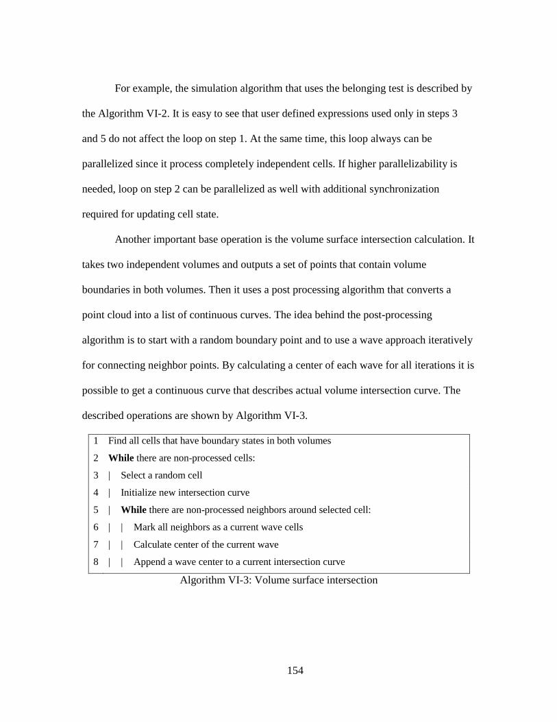
154
For example, the simulation algorithm that uses the belonging test is described by
the Algorithm VI-2. It is easy to see that user defined expressions used only in steps 3
and 5 do not affect the loop on step 1. At the same time, this loop always can be
parallelized since it process completely independent cells. If higher parallelizability is
needed, loop on step 2 can be parallelized as well with additional synchronization
required for updating cell state.
Another important base operation is the volume surface intersection calculation. It
takes two independent volumes and outputs a set of points that contain volume
boundaries in both volumes. Then it uses a post processing algorithm that converts a
point cloud into a list of continuous curves. The idea behind the post-processing
algorithm is to start with a random boundary point and to use a wave approach iteratively
for connecting neighbor points. By calculating a center of each wave for all iterations it is
possible to get a continuous curve that describes actual volume intersection curve. The
described operations are shown by Algorithm VI-3.
1 Find all cells that have boundary states in both volumes
2 While there are non-processed cells:
3 | Select a random cell
4 | Initialize new intersection curve
5 | While there are non-processed neighbors around selected cell:
6 | | Mark all neighbors as a current wave cells
7 | | Calculate center of the current wave
8 | | Append a wave center to a current intersection curve
Algorithm VI-3: Volume surface intersection

155
It is important to notice that only step 1 of the described algorithm can be easily
parallelized but other steps are iterative and cannot be performed in parallel easily.
However, this should not be a problem since they always process a reasonably small
subset of all cells that represents a curve. There is also possible a situation when volume
surface intersection a represented by a surface and not a curve. This special case can be
detected by calculating a standard deviation of processing waves and should be processed
separately but it is not considered in this work.
Two main operations described above are enough for implementing most path
planning algorithms. However there were also developed some special algorithms for
solving the tool orientation selection problem. These algorithms will be discussed later in
this chapter.
Volume based parallel algorithms design methodology and limitations
As was mentioned before belonging test and volume intersection are main tools
for working with the developed geometry representation. But solutions for most tool path
planning problems should be reformulated in a way that allows expression of these
solutions with available tools. For example a simple iso-planar [3-5] approach that uses
intersection between a sequence of parallel planes and a part surface as contact point
curves, can be easily implemented in a parallel fashion in two ways. First, intersection
between part surface and planes can be represented as intersection between part volume
and a sequence of parallelepipeds. Second, the belonging test can be applied where a
target shape is actually a sequence of plains. Although both approaches do the same task,

156
they are quite different and use different tools. But they both have two important benefits.
First, there is no need to care about special cases, singular points, discontinuities, etc.
Second, both approaches can be implemented in a highly parallel way and run on highly
parallel hardware.
The most important concept is to reformulate operations with surfaces by
operations with volumes that can be represented by independent operations with
volume’s cells. This reformulation guaranties that a new algorithm can be easily
parallelized. It also makes algorithms simpler since there is no need to handle special
cases anymore. Although reformulation of algorithms in volumetric fashion is usually not
too complicated, this approach requires caution due to some limitations of the underlying
discrete geometry representation.
The first important and probably the most dangerous limitation is related to the
volume boundary position. It is important to accept the fact that an actual surface position
is never perfectly known. The reason for it is a fact that a surface is represented by cells
that have very little information about what happens in them. Precisely each cell stores
only 2 bit of information that represent 3 states and only 2 of 3 states are guaranteed. If
cell has a completely empty state, it is guaranteed that it does not have any material
inside and vice versa for a completely full cell. But if a cell does not hold any of these
states, there is no guarantee that it actually contains a surface. In most cases and for most
applications it is safe to assume that such cell actually contains a surface. However even
if cell does contain a volume surface there is no way to know where a surface lies inside
of a cell. In most cases, especially for roughing planning application when removing few

157
tens of microns of material more or less does not really matter, the precision provided by
a cells size itself (since surface positioning error is limited by cell dimensions) is enough
for valid tool path planning process. But for finishing and especially high precision
finishing path planning additional tool path corrections may be needed.
The second limitation is related to the derivatives calculation. It is important to
eliminate using derivatives or assume that their accuracy is not perfect. Since the
underlying geometry representation has a discrete nature, derivatives calculation cannot
produce perfectly accurate results in many cases. However approximate derivatives
values can be calculated and used if they are needed. For example, surface normals used
in the rendering process for lightning calculations are actually estimated from a discrete
geometry representation in runtime and still provide good enough precision for rendering
accurate images.
Offset volume calculation
Despite the described limitations, many complex geometrical problems can be
easily solved by following the described approach. One of these tasks is the offset surface
finding problem. The offset surface is defined as a surface at equal distance from an
original surface (Figure VI-1). It is often used in tool path planning process as a surface
where a tool center may move freely without producing overcuts. By replacing tool
contact point trajectory planning with tool center trajectory planning it is possible to
eliminate a complicated gouge prevention process and make tool path planning
algorithms simpler.

158
Figure VI-1: Offset surface [65]
Although the offset surface makes path planning algorithms simpler, finding an
offset surface is not a trivial problem for analytical geometry representations. Most
common problems of this process are special cases such as holes and self-intersections
[66] as shown Figure VI-2. The developed offset surface finding approach eliminates the
self-intersection problem completely and allows using models with holes that are smaller
than offset distance. It is important to notice that the developed approach uses triangular
meshes as an input geometry representation but similar algorithms can be implemented
for other data structures. The reason for selecting the triangular mesh format is the weak
support of this format in modern CAM software and its popularity in RP industry.
Figure VI-2: Offset surface self-intersections [66]
The main idea behind the developed surface offset algorithm is working with
volumes and not with surfaces, so it is more correctly to describe it as the “offset

159
volume” algorithm. Here the offset volume represents a volume that contains all points
that are closer than an offset distance to initial surface. At the same time, it is easy to see
that a boundary surface of the offset volume contains a target offset surface and an offset
surface calculation can be replaced by offset volume calculation. In 2D case an offset
curve calculation can be replaced by offset area calculation as shown on Figure VI-3.
Figure VI-3: 2D offset surface decomposition
In order to construct an offset volume efficiently, it can be represented as a
composition of primitives associated original surface elements. For 2d case (Figure VI-3)
every point is associated with a circle and every line is associated with a rectangle. For 3d
model and triangular geometry representation there is a similar association list:
Vertex – Sphere
Edge – Cylinder
Face – Prism
As a result a triangular mesh may be converted in a list of volumetric primitives
that can be composed together and represent an offset volume. Then every cell of
geometry model can be tested against this list of volumetric primitives and marked as a

160
part of an offset volume if it passes belonging test with one of these primitives. The offset
volume calculation algorithm that combines all these steps is shown by Algorithm VI-4.
1 For all vertexes in input model in parallel:
2 | Add appropriate sphere to primitives list
3 For all edges in input model in parallel:
4 | Add appropriate cylinder to primitives list
5 For all faces in input model in parallel:
6 | Add appropriate prism to primitives list
7 For all cells in geometry model in parallel:
8 | For all primitives in list:
9 | | If cell belongs to primitive:
10 | | | Mark cell as an offset volume cell
Algorithm VI-4: Volume offset calculation
Loops 1, 3, 5 of the described algorithms are completely independent and can be
easily parallelized. Loop 7 is actually a part of the belonging test described before and
can be easily parallelized as well since all cells are always completely independent in the
developed geometry model. Even loop 8 can be parallelized with an additional
synchronization required for the cell updating process. It is obvious that the selected
approach can be parallelized in many ways but the implemented version is parallelized
only in step 7. Everything else is done sequentially, and there are few reasons for this.
First, with a high enough number of cells (which happens almost always for high
resolution models), there is no real need for higher level of parallelization. Second, steps
1-6 do not take too much time in any case. And finally, serial processing of primitives for
each cell allows stopping when a cell changes state first time and it saves a significant
amount of calculations.
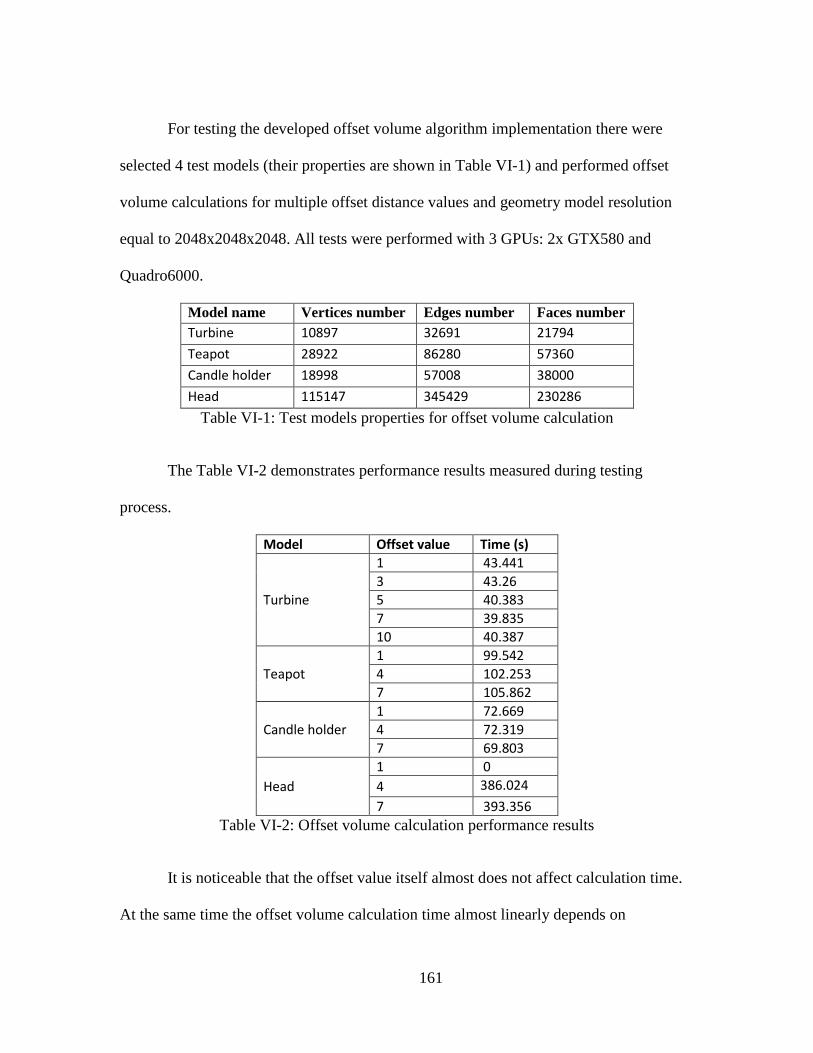
161
For testing the developed offset volume algorithm implementation there were
selected 4 test models (their properties are shown in Table VI-1) and performed offset
volume calculations for multiple offset distance values and geometry model resolution
equal to 2048x2048x2048. All tests were performed with 3 GPUs: 2x GTX580 and
Quadro6000.
Model name Vertices number Edges number Faces number
Turbine 10897 32691 21794
Teapot 28922 86280 57360
Candle holder 18998 57008 38000
Head 115147 345429 230286
Table VI-1: Test models properties for offset volume calculation
The Table VI-2 demonstrates performance results measured during testing
process.
Model Offset value Time (s)
Turbine
1 43.441
3 43.26
5 40.383
7 39.835
10 40.387
Teapot
1 99.542
4 102.253
7 105.862
Candle holder
1 72.669
4 72.319
7 69.803
Head
1 0
4 386.024
7 393.356
Table VI-2: Offset volume calculation performance results
It is noticeable that the offset value itself almost does not affect calculation time.
At the same time the offset volume calculation time almost linearly depends on

162
complexity of a geometry model. The Figure VI-4 demonstrates the offset volume
calculation performance in faces/second for all tried models and it is easy to see that
calculation speed is almost constant for all of them.
Figure VI-4: Offset volume generation performance
Pictures below demonstrate offset volume testing results for all test models.
0
100
200
300
400
500
600
700
1 3 5 7 10 1 4 7 1 4 7 1 4 7
Turbine Teapot Candle holder Head
Pe
rfro
man
ce, f
ace
s/s
Model and offset value

163
Figure VI-5: “Teapot” volume offset

164
Figure VI-6: “Turbine” volume offset

165
Figure VI-7: “Candle holder” offset volume
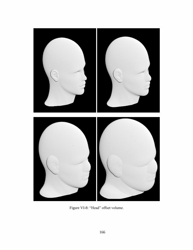
166
Figure VI-8: “Head” offset volume.

167
Surface filling algorithm based on 3D contour offset approach
The example of the offset volume calculation algorithm has shown that it is
possible to use the described earlier methodology and geometry representation for
solving computational geometry problems. This part will talk about problems that are
more closely related to tool path planning process itself.
First of all it is important to notice that modern CAM systems support a large
variety of tool path planning strategies (such as iso-parallel, spiral, contour offset, etc.)
that produce efficient tool paths for a variety of different situations. And although there
are so many possible options for tool path planning, these solutions are usually quite
specialized and do not work well as a true general purpose solution for any possible
situation. This limitation requires the presence of an engineer that select a sequence of
appropriate strategies with appropriate parameters and it has to be eliminated in order to
create a fully automated path planning system. One of possible ways for resolving this
problem is creating a system that can make decisions like an engineer and select the best
sequence automatically. However such a system should be quite smart and it should
support all known strategies in order to replace a human. It is obvious that the
development of such system will require a significant amount of time and it will be quite
useless before it is finished since there is no sense to use a program that can generate only
a portion of a tool path. The solution for this problem is development of a robust tool path
planning strategy that can take any possible geometry and produce a tool path for
machining it. It is obviously not possible to make this strategy optimal and efficient for
all cases but its goal is different. With such a strategy, development of a fully automated

168
tool path planning system will be much easier and useful because even if the developed
system cannot generate a complete tool path, it can always use the generalized robust
strategy for making a part. The robust strategy in this case becomes the foundation for a
fully automated tool path planning system. Such strategy was designed by following the
described methodology and implemented in this work. Before discussing the details, it is
important to notice that the developed version is designed especially for ball-end mills
but it can be improved for supporting other cutter types.
The idea behind the developed robust path planning strategy is generalizing the
2D contour offset strategy often used in modern CAM software to 3 dimensions.
Although 2D and 3D versions are conceptually similar (in fact a 2D version is a special
case of a 3D algorithm), there are some important differences related to where and how
they generate a tool path. Traditional contour offset approach calculates a tool path on a
plane which is orthogonal to a tool direction. It iteratively offsets a contour and uses
offset curves as tool path components. Usually a sequence of parallel planes is used for
removing most of volume during a roughing process. The 3D version does perform very
similar steps but does not require using a planar surface (although it can use a plane and
in this case it becomes a 2D contour offset approach). It uses any possible user selected
surface called “Target surface”. The problem here is an additional dimension. As a result,
offsetting a contour creates a tube like shape that cannot be used for path planning
(Figure VI-9b). As a solution for this problem, an additional step is required – calculation
of the intersection between a tube and a target surface (Figure VI-9c). By calculating the
intersection, it generates a curve that lies on a constant distance from an original contour

169
and can be used for further path planning. The important property of the contour offset
approach is preserved – the distance between path components is constant in most cases
and always bounded. This property allows controlling a scallop height of the machined
surface by controlling distance between path components.
a) target surface with initial curve
b) curve offset volume
c) intersection curve
d) offset volume of an intersection curve
Figure VI-9: Curve offsetting
Iterative performing of the contour offset algorithm until an entire surface (or a
surface part) is covered (Figure VI-10) generates a sequence of curves that completely fill
a target surface and that are further than the offset distance to each other. The developed
implementation determines that an entire surface is processed if it is not possible to
calculate intersection between curve offset volume and a target volume. It is also
important to notice that curve offset volume combines all offset volumes calculated

170
during previous iteration, so if a part of a target surface is already processed it will not be
processed again.
Figure VI-10: Iterative surface area filling
Before describing the complete surface filling algorithms it is important to talk
about the third component used in this process – restriction volume. Boundary conditions
and also any required restrictions are represented as a restriction volume that contains
areas where tool movements are not desired or dangerous. For example, during roughing
path planning for ball end tool, restriction volume includes a part offset volume with an
offset value equal to a tool radius. By not allowing path planning in areas that are too
close to a part surface, it predicts overcuts because a tool center will never come closer
than a tool radius and a tool surface will never intersect a part surface as a result. A
restriction volume also limits filling algorithm in a way that only a desired part of a
surface is processed even if an entire surface is not processed yet. This is useful for
protecting fixtures from accidental machining. For example, Figure VI-11 demonstrates

171
the restriction volume for the “Head” model that contains two parts: offset volume of the
model with offset distance equal the tool radius and a box volume in the bottom for
protecting fixtures.
Figure VI-11: Restriction volume for the “Head” model
The entire surface filling process is described by Algorithm VI-5.
1 Current curve = Initial curve
2 Do:
3 | Offset current curve
4 | Calculate Intersection curve between Target surface and Offset volume
5 | If intersection curve exists:
6 | | Save intersection curve as a tool path component
7 | | Current curve = Intersection curve
8 Until: Intersection curve does not exist
Algorithm VI-5: Surface filling
The most important property of the developed surface filling algorithm is
parallelizability. Since it is based on volume offset (curve offset algorithm, which is
actually used, is a special case of volume offset algorithm described earlier) and volume

172
intersection algorithms which are both parallel, the entire surface filling algorithm
becomes naturally parallel and all algorithms that use it are also naturally parallel.
Robust tool trajectory generation for 5-axis machines
The described 3D contour offset algorithm is used both for the roughing and the
finishing tool path planning by using different target surfaces. In case of finishing a
model offset volume surface is used as s target surface. An offset value in this case is
equal a tool radius. And a contour offset value controls path step and it is selected based
on a desired scallop height. As it was mentioned before, limiting tool center movements
to an offset surface prevents overcuts by a ball part of a tool. For the finishing path
generation, an initial curve can be selected in many ways but the current implementation
uses an intersection between a horizontal plane and a top of an offset model.
The Figure VI-12 demonstrates an example of the surface filling process used for
a finishing tool path generation and Algorithm VI-6 demonstrates required algorithm
steps. Intersection curves calculated during this process are used as tool center trajectory
curves in a finishing tool path.
1 Calculate intersection curve between part offset volume and horizontal plane
2 Apply the Surface filling algorithm starting with the intersection curve (Algorithm
VI-5)
3 Generate a finishing tool path by combining all generated curves
Algorithm VI-6: Finishing tool path generation

173
Figure VI-12: Surface filling for finishing tool path generation
The roughing tool path generation process is a bit more complicated than the
finishing process because it has to process a volume, not a surface. There are three main
differences. First, it uses iterative approach and generates a tool path that removes
material layer by layer until it reaches a part surface. Second, a target surface for
roughing process is a workpiece material surface itself. Similarly to the finishing process,
it uses surface filling algorithm for generating a set of curves on a material surface that
are used as tool center trajectory curves. And finally, roughing algorithm selects initial
curves differently. The current implementation uses the intersection between a workpiece
and a model offset volume for selecting an initial curve. After the intersection is

174
calculated, the longest intersection curve is selected (Figure VI-13) and the surface filling
algorithm is used. This process repeats until all intersection curves are processed and it is
not possible to find a curve that lies outside of a safety zone. All roughing path planning
steps are demonstrated by Algorithm VI-7.
Figure VI-13: Initial curve selection for roughing process
1 Calculate part and fixtures offset volume (Algorithm VI-4)
2 Do:
3 | Calculate intersection curves between workpiece and part offset volumes
4 | While non-processed intersection available:
5 | | Select the longest intersection curve
6 | | Apply the Surface filling algorithm starting with the selected curve
7 | | Generate a roughing tool path for a layer by combining all generated curves
8 Until intersection curves exist
9 Generate a roughing tool path by combining all layers
Algorithm VI-7: Roughing path planning

175
The Figure VI-14 demonstrates workpiece geometry after removing each layer of
material during a roughing process with a tool path generated by the described roughing
algorithm. It is also easy to see exact tool trajectory on the first few layers.
Figure VI-14: Layer by layer material removing during a roughing process.
The described finishing and roughing tool path planning approaches have some
important properties that should be mentioned. First of all, these algorithms follow the
developed methodology and mainly perform volume offset, volumes intersection and
176
surface filling operations. Since all these operations are naturally parallel, all developed
tool path planning algorithms hold this property. The second important property is
robustness. In context of this work, robustness means an ability to generate a valid tool
path for any given geometry. It is easy to see that both algorithms just perform a set of
steps without knowledge about geometry itself so they are geometry agnostic and can be
applied to any possible part. It is also easy to see that both algorithms stop to work only
when they process an entire surface or volume since it is part of existing conditions.
These properties make the described algorithms great candidates for a foundation
of a completely automated tool path planning platform because even if an optimal
algorithm for geometry is not known, these algorithms can always generate a tool path.
However it is important to remember that in most cases they do not provide an optimal
result, and that they should be used as a last resort.
Orientation selection
The previous part described algorithms that are capable of generating a tool center
trajectory that results in machining of a desired geometry. But a tool center trajectory is
only a part of a tool path for 5-axis machines since there is a need for a valid tool
orientation at each point. This work makes an important assumption: tool orientation can
be calculated independently after calculation of a tool trajectory. Although this
assumption does not always work and probably does not allow generating an optimal tool
path for all possible scenarios, it works in most cases and significantly simplifies a tool
path planning process by decomposing it into two independent process of trajectory and

177
orientation planning. It is also important to notice that in spite of the assumption made,
the implemented tool path planning system generates orientation for each layer of a
roughing path planning process and as result orientation planning on each layer actually
does affect trajectory planning on a next layer. For example if some volume cannot be
removed on a layer because it is not possible to select a collision free orientation for a
tool path, it may become possible on future layers because there are less constraints due
to removed volume.
Before discussing a tool orientation selection process, it is important to mention
that it heavily depends on a concept of accessibility map that represents all collision- and
gouge-free orientations for a given tool center position (cutter contact point can be used
as well with minor changes but it is not discussed in this work). An accessibility map is
stored as a bitmap where each pixel represents two rotary axis coordinates and has a
value of 0 if this is a valid orientation or value 1 if this orientation results into collision as
shown on Figure VI-15. A description of a highly parallel efficient algorithm for
accessibility map calculation will be provided later in this work. Although this algorithm
does not include a prediction of machine components collisions, there is an assumption
that it is possible to calculate an accessibility map with a high enough resolution in a
reasonably short time for any given point.
Figure VI-15: Accessibility map example
A
C Angles limited
to this area

178
It is also important to describe the desired orientation properties used in this work.
Since there are infinite possible tool orientations, selection of tool orientation can be
viewed as an optimization process with constraints represented by accessibility maps
(machine dynamics constraints are not considered directly in this work) and a selected
optimization criteria that represent desired orientation properties. In this work a smooth
orientation change is selected as a target tool orientation property. The idea behind this is
to be as continuous as possible, and to use as low speed rotary axis movements as
possible. This can be described as true 5-axis machining which usually happens during
machining complex true 5-axis parts. There was an assumption that solving a tool
orientation problem for this scenario will allow solving orientation problems for simpler
3+2 axis cases by adding more constraints.
The developed orientation selection system uses an assumption that orientation
selection happens after tool trajectory planning and 3 of 5 axis values are already known
for each tool path point, so there is a need to find only 2 more axis values. An orientation
of each tool trajectory point can be described as a 2D point in orientation space and
orientation for all tool path points can be described as a set of 2D points. Considering the
fact that orientation change physically means a continuous rotary axis movement, tool
orientation change during following a tool trajectory should be continuous and can be
described as moving a point on a 2D curve. Movement of a 2D point brings a 3rd
dimension that can represent either a time or a distance from the beginning of tool center
trajectory. There is obviously no difference from a mathematical point of view between
point movement on 2D curve and a curve in 3D space but the last one is better from a

179
constraints visualization point of view. Since every tool center point has a different
accessibility map, an orientation selection process can be viewing as construction of a 3d
curve that goes through a stack of accessibility maps (Figure VI-16).
Figure VI-16: 3D curve going through a stack of bitmaps
The implemented version of the orientation selection algorithm actually works by
constructing a curve through a stack of accessibility map. It uses a two stage process:
first, it selects an optimal accessibility space topology; second, it generates an initial
curve, by selecting points that lie as far as possible from borders, and iteratively optimize
a curve shape for making it smooth.
The first step is needed for reducing the number of tool retractions due to
impossibility of continuous orientation change (these retractions will be called “jumps”).
Jumps happen when a tool center position can be accessible only from orientations that
cannot accessed by continuous rotary axis movement from a position that was selected

180
for a previous tool center position. In this case a tool is retracted, orientation is changed
and a tool center is moved to the next tool center position.
Figure VI-17: Example of a tool trajectory that requires a tool retraction
For example, as shown on Figure VI-17, if a tool center follows the showed
trajectory, earlier or later it will not be able to continue without a jump. It is important to
notice that the last point where tool can go without a jump depends on a tool movement
direction as shown on Figure VI-18.
Figure VI-18: Dependency of a jump point on tool movement direction
The shown example is a simple case when only one jump is done and required.
But, even with this example, it is already possible to notice that this situation is a

181
limitation of the earlier assumption about the independency of a tool trajectory planning
process and orientation selection. It is easy to see that an entire surface of the
demonstrated teapot can be processed without any jumps if a different tool trajectory is
selected. However in many situations jumps are not avoidable at all. In these cases a tool
path planning algorithm can try to minimize a number of jumps because tool retractions
increase total machining time and also may decrease a tool life by increasing a number of
tool load changes. For example, in situation shown on Figure VI-19 there are 2 possible
ways for selection a tool orientation if a tool follows a straight line trajectory as shown on
Figure VI-20.
Figure VI-19: A scenario with a complicated tool space topology
Figure VI-20: Two possible ways of orientation selection

182
It is easy to see that the left way requires two jumps and the right one requires
only one jump and it probably should be selected. In order to understand how the right
way can be selected it is important to look on an accessibility space that shows all valid
tool orientations. For a 5-axis machine with 2 rotary axises, an accessibility space has 3
dimensions (2 axis + time). But in order to simplify explanation and visualization an
assumption is made that there is only 1 rotary axis (around and axis that lies in a wall
plane perpendicular to a tool path line on Figure VI-20) and an accessibility space has 2
dimensions (accessibility map accordingly has only 1 dimension in this case). In this case
an accessibility space for the described situation looks similar to Figure VI-21 where a
center line represents a tool orientation along a wall normal and grey area represents valid
orientations.
Figure VI-21: Accessibility space
The Figure VI-22 provides an explanation of a construction process for the
accessibility map shown on Figure VI-21. The top part of it demonstrates a top view on a

183
target part. The accessibility space is located in the bottom and divided into 5 zones
accordingly to a possible combination of orientations in each zone. Approximations of
accessible zones are marked by blue rectangles. Finally, considering the fact that a tool
moves continuously, black lines represent corrected accessibility area borders.
Figure VI-22: Explanation of an accessibility map construction process
Before the explanation of the optimization process, it is impossible to explain how a jump
looks in accessibility map space. Considering that a jump always happens for exactly the
same tool center orientation, it means that it always happens in a vertical slice of the
accessibility space. As a result it can be viewed as a rapid movement from one
accessibility zone to another (

184
Figure VI-23). Where an accessibility zone is a part of the accessibility space for a given
tool center position that includes all points that can be accessible by continuous
orientation change. It is important to notice that accessibility zone always has the same
number of dimension as an entire accessibility space.
Figure VI-23: “Jump” concept explanation
The developed topology optimization approach is based on the idea of
representation of an accessibility space as a graph of connected accessibility zones and
searching for a shortest path. It is easy to see that an accessibility space can be discretized
by slicing it into a sequence of accessibility map (the developed implementation actually
works in an opposite way, it generate a sequence of accessibility map and constructs an
accessibility space from them). Each accessibility map will have a set of accessibility

185
zones that can be connected based on possibility of moving from one zone to another as
shown on
Figure VI-24. Two accessibility zones can be connected only if they intersection
is not empty. From a machining point of view it means that a tool can move from one
tool center position to another without changing a tool orientation.
Figure VI-24: Accessibility space slicing and connection
It is easy to see that accessibility zones can be viewed as nodes of a graph that
represent an accessibility space topology. However, it is not possible to find a path from
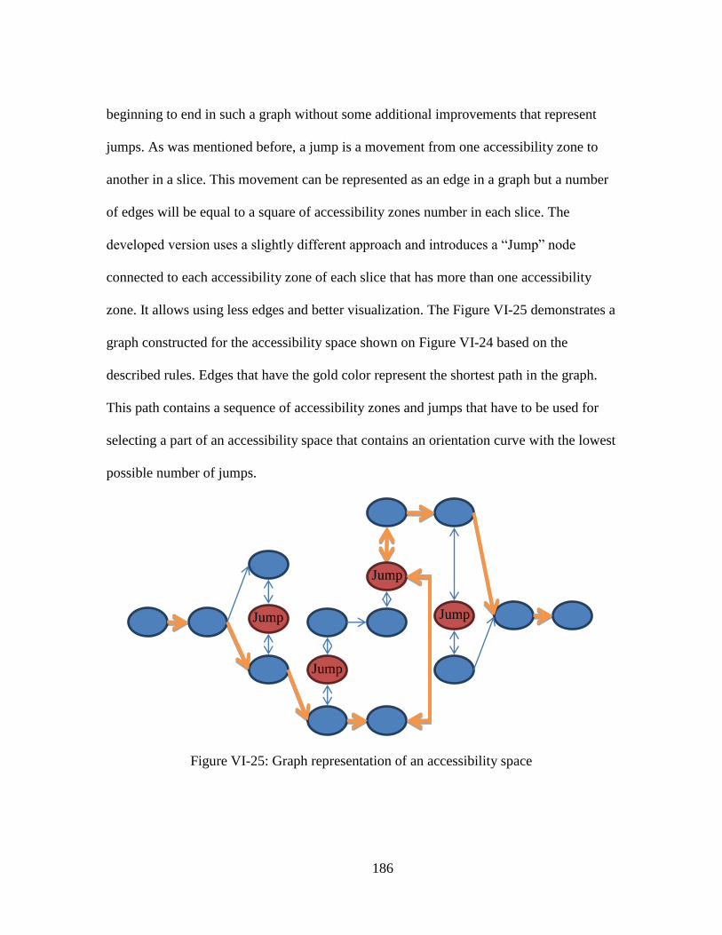
186
beginning to end in such a graph without some additional improvements that represent
jumps. As was mentioned before, a jump is a movement from one accessibility zone to
another in a slice. This movement can be represented as an edge in a graph but a number
of edges will be equal to a square of accessibility zones number in each slice. The
developed version uses a slightly different approach and introduces a “Jump” node
connected to each accessibility zone of each slice that has more than one accessibility
zone. It allows using less edges and better visualization. The Figure VI-25 demonstrates a
graph constructed for the accessibility space shown on Figure VI-24 based on the
described rules. Edges that have the gold color represent the shortest path in the graph.
This path contains a sequence of accessibility zones and jumps that have to be used for
selecting a part of an accessibility space that contains an orientation curve with the lowest
possible number of jumps.
Figure VI-25: Graph representation of an accessibility space
Jump
Jump
Jump
Jump

187
The developed implementation of the discussed algorithm uses the “NetworkX”
Python library for managing a graph structure and searching for the shortest path in a
graph (“Dijkstra's algorithm with Fibonacci heap” [67] with O(E+V*logV) complexity)
and implements the graph construction process described by the Algorithm VI-8.
1 Calculate accessibility map (AS slices) for each tool center point (Algorithm VI-11)
2 For all accessibility maps:
3 | Find all accessibility zones (AZ)
4 For all accessibility zone:
5 | Add a node to a graph
6 | For all accessibility zones on a previous slice:
7 | | If intersection between AZ on current layer and previous layer exist:
8 | | | Add an edge
9 For each slice:
10 If there are more than one accessibility zone:
11 | Add “Jump” node and edges from this node to all AZ in this slice
Algorithm VI-8: Accessibility graph construction
It is important to note that the developed version of the described algorithm
actually works with 3D accessibility space in opposite to the described 2D case. Although
a number of dimensions is different, it implements conceptually the same ideas of
representing an accessibility space as a graph and search for the shortest path. An
example of a real life accessibility space graph is shown on Figure VI-26 (node values
represent a number of an accessibility zone in a slice).

188
Figure VI-26: Real life example of an accessibility map graph
The next step in the orientation planning process is the construction of an
orientation curve in a selected part of the accessibility space. Before the construction of
an actual curve, an accessibility space should be reduced by using only accessibility
zones represented by the shortest path in a graph. At this point a tool path is also divided
into a sequence of segments corresponding to segments of nodes in the shortest path.
Since there are jumps between these regions, tool orientation at ends of these segments
can be selected independently and it does not make sense to optimize them together. As a
result it is possible to reduce a length of a curve that has to be optimized at once. The
curve construction process has two main parts: construction of an initial curve and
iterative optimization.

189
Generally, an initial curve can be selected randomly if a stable optimization
algorithm is used but, as with any other optimization techniques, a good initial guess
results in much faster convergence. The developed accessibility curve construction
system generates a curve from points that lie as far as possible from border of
accessibility zones. The developed implementation uses the “Distance transform”
algorithm [68] (with O(N2) complexity) implemented in OpenCV library in order to find
these points. The distance transform algorithm calculates an approximate distance to the
closes zero pixel of a given bitmap. As a result, a pixel with the maximum distance value
represents the furthest point from an accessibility zone boundary. As a result, an initial
curve is constructed by applying a distance transform to all accessibility maps and using
points with maximum distance values. Although the described way guarantees that all
accessibility curve points lie inside accessibility zones, there is no guarantee that an entire
curve lies in accessible area because some curve segments between initial points may lie
in non-accessible areas. A solution for this problem is the developed implementation is
applying Boolean “And” operations between all neighbor accessibility maps before
construction of an accessibility space graph. Although it reduces an accessibility space
and can result into impossibility of a tool path construction, this situation is not likely.
However if Boolean “And” produces an empty map, this will mean that it is dangerous to
machine this area since a tool will be very close to a part. As a result, it will be treated as
an inaccessible area and the tool path planning algorithm will try to machine it later when
more material is removed and the area may become accessible.

190
The complete process of preparing of an accessibility space and an initial curve
construction is described by Algorithm VI-9.
1 Calculate the shortest path in an accessibility space graph
2 Remove all accessibility zones that are not part of the shortest path
3 For all accessibility zones:
4 | Apply a distance transform
5 | Find a point with maximum distance value
6 | Add found point to an initial curve
Algorithm VI-9: Initial accessibility curve construction
After generating an initial curve, the last part of the accessibility curve
construction is an iterative optimization. The implemented optimization approach is quite
simple and tries to smooth a curve as much as possible while staying in accessible area.
For simplicity of an algorithm explanation, there is an assumption that an accessibility
curve has only 2 dimensions. The actual system works with 3 dimensional curves since it
is designed for 5-axis machines, but it uses conceptually the same algorithm.
A 2D curve can be represented by 1D array of floats (as it is done in a height map,
Figure VI-27) under assumption that all curve points are evenly spaced, which is correct
since they are located on accessibility space slices in the developed system. Before
continuing the optimization part it is possible to note that although the idea of slicing an
accessibility space is a good way to deal with it, selecting equal space between slices in
some cases is inefficient and bring a lot of problems. It is possible to recommend that
dynamic accessibility space subdivision with non-constant slices density is a better
approach that may save a significant amount of memory. But the actually implemented

191
orientation system uses constant distance between slices and all following explanation
will be done based on this fact.
Figure VI-27: Curve representation
The first step of optimization iteration is calculation of a gradient by using the
formula (VI-1).
(VI-1)
Where “ ” is a coordinate of ith point and “k” is a damping coefficient used for
prevention oscillation. The used value for the “k” is 0.9. After calculating gradients for
each point (except first and last points which are always locked at their initial positions),
a new point position is calculated:
(VI-2)
If the new position lies inside accessible zone, a point position is updated by a
newly calculated value. However if a new position is not a valid orientation, a point is not
moved. The developed orientation curve optimization system performs described
iterations continuously during a given time that is based on a curve length. Using a time
Y0
Y1 Y2
Y4
Y5
Y3
Y6 Y7 Y8 Y9
Y
X

192
limit as a single stopping condition was selected for simplification of the development
process and better control over optimization time.
1 Calculate an initial accessibility curve
2 While time limit is not reached:
3 | For each point in a curve:
4 | | Calculate gradient
5 | | Calculate next position
6 | | If next position is in accessible zone:
7 | | | Update point position
Algorithm VI-10: Accessibility curve optimization
The Algorithm VI-10 demonstrates steps performed during an accessibility curve
optimization process.

193
Figure VI-28: 3D curve optimization example
The Figure VI-28 demonstrates an example of a real 3 dimensional accessibility
curve optimization. It is important to remember that this curve has 3 dimensions and is
calculated for 5-axis machine with a continuous C axis, so it is normal to see rapid
movements from one end to another. These movements are just a visualization of the
continuous axis rotation and going from 359 to 0 degrees.

194
Figure VI-29: Accessibility space (views from multiple camera positions)
The Figure VI-29 demonstrates an example of a 3D accessibility space. On the
picture, borders between accessible and non-accessible areas for each accessibility zone
are represented by tubes. This accessibility space is calculated for the first few segments
of a roughing path that process a cube of material. A real world example of an
accessibility curve constructed in accessibility space is shown on Figure VI-30 - Figure
VI-32.

195
Figure VI-30: Accessibility curve going through accessibility space, view 1
Figure VI-31: Accessibility curve going through accessibility space, view 2

196
Figure VI-32: Accessibility curve going through accessibility space, view 3
Accessibility map generation
It was mentioned above that all orientation selection algorithms are based on an
assumption that there is a known accessibility map. This part describes an algorithm
developed for computing accessibility map for a given point and a given tool/holder
combination. Most of research project related to orientation selection [69, 70] are based
on a concept of accessibility (or visibility) cone [71]. The problem with this approach is
the simplification of an accessibility map by a cone or a set of cones. Although it is often
a good enough approach that saves a lot of memory and computational resources, it does
not provide an accurate representation of a real accessibility map.
The developed approach is based on the completely opposite idea of using
inaccessibility cones calculated for each geometry model element independently.
Considering the fact that the developed geometry representation uses a set of spherical
cells for representing a volume, it is possible to say that a valid orientation is an
orientation that does not result in a collision with any of cells. So if it is possible to find

197
all orientations that result into collision for each cell, all collision prone orientations will
be described by a union of collision prone orientations of each cell and all collision free
orientation will be described by a complement of that union. Independence of cells and
their collision prone orientation also allows calculation of these orientations in parallel
which is an important property for this work. An interesting part here is the calculation of
inaccessible orientations for a spherical cell and a give tool and tool holder combinations.
It is easy to see that for a fixed tool center position and a given spherical cell, a tool may
come to a cell as close as possible until their surfaces touch each other as shown on
Figure VI-33. It is also possible to calculate the angle between a tool orientation and a
vector from tool center to a sphere center.
Figure VI-33: Touching a cell surface by a tool surface

198
It is also obvious that a tool may touch a sphere from many different sides as
shown on Figure VI-34 but an angle between tool direction and a vector to a sphere
center is constant in all cases.
Figure VI-34: Touching a sphere from multiple sides
By looking on all possible tool orientations when a tool center is fixed and tool
touches a sphere as shown on Figure VI-35, it is possible to see that the tool direction
vectors make a cone around the vector to a sphere center.

199
Figure VI-35: All tool orientation when a tool touches a sphere
This cone is called an inaccessibility cone since all tool directions that lie inside
of this cone result into a collision. If given the tool center, the sphere center and the tool
geometry, the angle between the cone center line and the cone surface can be calculated.
Since a cone center line is a vector between a tool center and a sphere center, and a cone
top is a tool center, this angle completely determines an inaccessibility cone. Since an
Inaccessibility Cone Angle (ICA) is a single dimension value, there is no need to
consider 3D space and an explanation can be done in 2D by using a 2D tool model shown
on Figure VI-36.

200
Figure VI-36: 2D tool model
An ICA has two components related to a spherical cell itself and tool geometry as
shown on Figure VI-37. The spherical part of an ICA is needed since a cell is actually a
sphere, rather than a point. So this part represents an angle between a cell center and a
cell tangent.
Tool offset
line
Spherical cell
-radius
( )-center
Circle with center
at tool center
Tool
surface
Tool center
line
( )

201
Figure VI-37: Inaccessibility cone angle components
The second component can be easily calculated by formula:
√
Where ( ) – k-th cell center and cell radius.
The first part, which is related to a tool and tool holder geometry, is a bit more
complicated. It is also important to mention here that for safety reasons, a tool surface
offset is used instead of a tool surface itself. It allows controlling the gap between
material and a moving tool during a machining process by changing surface offset value.
Calculation of the first ICA components is a bit more complicated. It is defined as
an angle between a tool center line and a vector to a sphere center when a sphere center
1
2

202
lies on a border of a tool. Here an assumption should be made that the developed
approach does not support a situation when a tool has complex shape that allows so that it
is possible to have a material between tool surface and a tool centerline. Considering this
assumption and the fact that a tool model has many components, the first ICA
components can be found as a maximum angle between tool center line and a vector to an
intersection between tool offset components and a circle with a center at tool center and
radius equal to a distance to a sphere center. This can be calculated with formula:
| |
Where vector to p-th intersection between tool surface offset components and
a circle around tool center that intersects a cell center and – tool center line. As a result
the ICA for a k-the cell can be defined as:
√
| |
Now, when ICA can be calculated, it is possible to write a complete mathematical
definition of an accessibility map. It can be represented as a matrix of Boolean values
with resolution (n, m):
[
]
Where each matrix element with coordinates (i, j) represent a tool orientation
defined by angles:

203
All matrix elements can be calculated as:
⋂( )
Here the is an ICA defined earlier and is an angle between a tool
orientation vector associated with a matrix element and a vector to a k-th cell center. This
vector is defined by following formulas:
| |
=( )
( )
√
From a computational point of view, the implemented version uses OpenCL and
runs all calculations on multiple GPUs by following the Algorithm VI-11. It calculated
all ICA in parallel first and then calculates all accessibility map elements in parallel as
well. Calculation of a single AM with resolution 256x512 takes approximately 20-40ms.
1 For all cells in parallel:
2 | Calculate ICA
3 For accessibility map element in parallel:
4 | For all cells in parallel:
5 | | Calculate angle between represented direction and cell center
6 | | If calculated angle is less than ICA:
7 | | | Mark map element as inaccessible
Algorithm VI-11: Accessibility map calculation

204
The developed accessibility map calculation approach has shown great
parallelizability and scalability as well as a quite good performance. In opposition to the
other accessibility map calculation techniques mentioned earlier, it does not use any
simplifications of an accessibility space and produces very accurate accessibility maps.
However since there are no simplifications used, it uses significantly more memory for
the storing accessibility map.
Another important property of the developed algorithm is an ability to use a
complete tool and tool holder geometry representation without any simplifications. It
allows considering all parts of a tool and holder and using orientations that are safe but
not defined as safe for other methods due to simplified tool geometry representation.

205
High level tool path planning control algorithm
The previous parts have described all components required for creation of a
complete robust tool path planning strategy that can produce a valid result. But it is
important to show a high level algorithm that brings all components together into a path
planning system. This algorithm is shown by the Algorithm VI-12.
1 Offset target geometry and fixtures volumes for roughing tool (Algorithm VI-4)
2 Do:
3 | Generate roughing tool path for layer (Algorithm VI-7)
4 | Generate accessibility map for each point (Algorithm VI-11)
5 | Optimize accessibility space (Algorithm VI-8)
6 | Construct initial accessibility curve (Algorithm VI-9)
7 | Optimize accessibility curve (Algorithm VI-10)
8 | Simulate generated tool path (Algorithm V-1 & Algorithm V-2)
9 While generated tool path length is greater than zero
10 Offset target geometry and fixtures volumes for finishing tool (Algorithm VI-4)
11 Generate finishing tool path (Algorithm VI-6)
12 Perform steps 4-7 for the finish tool path
Algorithm VI-12: High level control algorithm
Experimental 5-axis milling results
All described tool trajectory and orientation planning algorithms were
implemented in Python, C++ and OpenCL languages during the research project. The
developed system was tested on a computer with 3 GPUs and showed great
parallelizability and scalability very similar to performance result showed in the previous
chapter describing 5-axis milling simulator. This chapter will not provide additional

206
performance details for three reasons. First, both the simulation and the low level part of
the path planning system use exactly the same implementation of the geometry
representation and processing core. As a result, they have exactly the same level of
parallelizability shown in the previous chapter and there is no need to show the same
results. Second, high level path planning algorithms heavily depend on input geometry
from the amount of calculations point of view. It means that all performance testing
results will be valid only for test geometry models. And finally, the developed version
uses a lot of reasonably slow Python code that can be much faster if it is rewritten in
C++. In spite everything mentioned above, it takes about 10-20 minutes to generate a
complete tool path for all tested models, so it can be stated that after performance tuning
and code improvement it will take less than 10 minutes for generating a valid tool path
for any given model.
In order to validate developed methodology and algorithms, the developed path
planning system was used for generation G-code programs for multiple parts. These G-
code programs were tested in both virtual and real environments on the developed 5-axis
machining simulator and Okuma MU500VA 5-axis milling machine.
The process of converting of a tool path into a G-code program is done by the
post-processor software. Commercial CAM systems usually include a generalized post-
processor that can be configured for a particular CNC controller but they require using a
special tool path description language. Since converting a tool path into a post-processor
language is more complicated (due to the lack of documentation) than converting it into
the G-code format itself, there was developed a simplified post-processor designed for

207
the used Okuma machine. It converts tool motions in the developed software format
directly to G1 commands and use some simple program optimization such as combining
collinear motions or removing constant components in order to reduce size of an output
program.
The following pictures demonstrate simulation and machining results for various
test models and materials.

208
(15 minutes planning type; 3 hours machining time)
Figure VI-38: Test model “Head”

209
(15 minutes planning type; 1.5 hours machining time)
Figure VI-39: Test model “Fan”
(10 minutes planning type; 1.5 hours machining time)
Figure VI-40: Test model “Puppy”

210
Discussion
This chapter has described the developed design methodology for a highly
parallel algorithm and a set of tool path planning algorithms developed by following the
methodology. These algorithms include a solution for common computational geometry
problems, such as offset surface calculation or volume surface intersections and a set of
robust algorithm for multi-axis tool path planning used in CNC milling. Following the
design methodology and using the developed highly parallel geometry representation
have resulted in high parallelizability and scalability of these algorithms. As a result, they
can efficiently run on multi-GPU systems with more than a thousand cores.
The developed path planning algorithms were combined in an automatic path
planning system capable of producing a valid G-code program for 5-axis CNC milling
machine with a very little guidance from a user. The developed path planning system was
tested in both a virtual and a real environment by generating G-code programs a running
them in the developed simulator and on a real machine.
The experimental results have proved that GPGPU approach can be used for
acceleration and automation of the tool path planning process for CNC milling machines.
Although the developed system often generates not the most efficient tool path, it can be
used as a foundation for a fully automated tool path planning system since it already
provides a set of very robust path planning algorithms that can generate a valid tool path
for almost any possible input geometry.
Although the developed system demonstrated good results, it is important to
remember that the implemented version of all path planning and accessibility map

211
generation algorithms is limited to the ball-end cutter only. It is also important that
remember that if a tool center point lies in inaccessible area, the developed path planning
system will just skip it and will not try to machine as close as possible. As a result, there
may be areas where material is not removed at all even if it was possible to remove
almost all material. And the most important limitation is the fact that the described path
planning algorithms were designed as robust and they do not provide the most efficient
tool path.

212
VII. CONCLUSIONS AND RECOMMENDATIONS
The first part of this work formulated the methodology for selection of a right
geometry representation and a data structure suitable for parallel processing on GPU.
Then the methodology was used for designing the 3-axis CNC milling simulation and
path planning algorithms accelerated with the GPGPU technology. The developed
algorithms were validated by performing 3-axis simulation and experimental machining.
The experimental results showed the importance of a highly parallel design and
demonstrate almost an order of magnitude difference between CPU and GPU
performance results.
The second part of this work generalized the developed methodology for
supporting multi-GPU systems and developed a completely new geometry representation
for designing algorithms capable of performing 5-axis CNC tool path planning and
simulation. Then the developed algorithms were verified by developing a fully automated
5-axis tool path planning system capable of producing valid G-code programs for any
geometry. Finally the developed system was used for the generation of test programs that
were tested in both virtual and real environments by running them in the developed 5-axis
CNC milling simulator and on a real 5-axis CNC milling machine.
The experimental results produced in this work proved that highly parallel
computing hardware (such as widely available and used in this work multi-GPU
computing system) and appropriate highly parallel algorithms can significantly expand
limits of modern tool path planning systems. The performance of parallel computing

213
allows implementing algorithms that were not considered before due to computational
requirements. And as a result, it allows further manufacturing automation that may create
completely automated manufacturing systems.
Although developed in this work algorithms and systems were successfully tested
and demonstrated good results, it is important to remember that there were made some
important assumptions and the developed solutions have many limitations. The most
important assumption made in this work is that it is possible to generate a good tool path
based just on geometric constraints without considering physical limitations. It is true in
most cases, but it will not work for machining some material such as titanium and there
will be a need to integrate physical limitations into a tool path planning process. Other
assumptions were made about optimization of a tool path. For example, it is assumed that
a tool orientation change should be as smooth as possible. Although it makes sense
sometime, it may be more appropriate to use a constant tool orientation with few rapid
changes. Some other limitations are more related to implementation of the developed
ideas and algorithms. For example, the developed path planning and accessibility map
generation algorithms are designed for the ball-end tool but it is possible to modify them
in order to support some other tool types such as flat-end or conic-end.
Considering the good results, it is possible to recommend continuing this research
project since there are still many areas that can be significantly improved. One of the
most important aspects from a practical point of view is the implementation of an
accessibility map algorithm that allows prediction collisions between machine
components. This improvement would make the machining process significantly safer

214
and allow using the full range of machine motions. The next important part is the
development of an expandable tool path planning system based on current robust path
planning algorithms. In this case, expandable means an ability to use multiple
implemented tool path planning strategies (that also have to be implemented in future)
and select them based on a part geometry analysis (feature detection and part subdivision
will be needed for this functional). Finally, it will be possible to create a tree of possible
solutions and at that point it would make sense to run a developed path planning system
on a cluster or cloud where each node processes an independent list of strategies used for
tool path planning. Development of all described features will eventually make it possible
to replace a human engineer completely and significantly reduce manufacturing the time
and cost as a result.

215
REFERENCES
[1] Centrifuge Brand Marketing Research, 2010, "Machine Tool Professionals, Outlook
on CNC Machine Investments," .
[2] Smith, K., Wang, A., and Fujino, L., 2012, "Through the Looking Glass: Trend
Tracking for ISSCC 2012," IEEE Solid-State Circuits Magazine, 4(1) pp. 4 - 20.
[3] BOBROW, J., 1985, "NC Machine Tool Path Generation from CSG Part
Representations" Computer-Aided Design, 17(2) pp. 69 - 76.
[4] HWANG, J., 1992, "Interference-Free Tool-Path Generation in the NC Machining of
Parametric Compound Surfaces," Computer-Aided Design, 24(12) pp. 667 - 676.
[5] LI, S., and JERARD, R., 1994, "5-Axis Machining of Sculptured Surfaces with a Flat-
End Cutter," Computer-Aided Design, 26(3) pp. 165 - 178.
[6] LONEY, G., and OZSOY, T., 1987, "NC Machining of Free Form Surfaces,"
Computer-Aided Design, 19(2) pp. 85 - 90.
[7] Suresh K, Y. D., 1994, "Constant Scallop Height Machining of Free Form Surfaces,"
Journal of Engineering for Industry, 9pp. 116-253.
[8] Rong-Shine Lin, Y. K., 1996, "Efficient Tool-Path Planning for Machining Free-
Form Surfaces," Transactions of the ASME, 118(1) pp. 20-28.
[9] Lasemi, A., Xue, D., and Gu, P., 2010, "Recent Development in CNC Machining of
Freeform Surfaces: A State-of-the-Art Review," Computer-Aided Design, 42(7) pp.
641 - 654.
[10] Lee, Y. -., and Ji, H., 1997, "Surface Interrogation and Machining Strip Evaluation
for 5-Axis CNC Die and Mold Machining," International Journal of Production
Research, 35(1) pp. 225 - 252.
[11] Lauwers, B., Kiswanto, G., Kruth, J. -., 2003, "Development of a Five-Axis Milling
Tool Path Generation Algorithm Based on Faceted Models," CIRP Annals -
Manufacturing Technology, 52(1) pp. 85-88.
[12] Giri, V., Bezbaruah, D., Bubna, P., 2005, "Selection of Master Cutter Paths in
Sculptured Surface Machining by Employing Curvature Principle," International
Journal of Machine Tools and Manufacture, 45(10) pp. 1202-1209.

216
[13] Han, Z., and Yang, D. C. H., 1999, "Iso-Phote Based Tool-Path Generation for
Machining Free-Form Surfaces," Journal of Manufacturing Science and
Engineering, 121(4) pp. 656.
[14] Ding, S., Mannan, M. A., Poo, A. N., 2003, "Adaptive Iso-Planar Tool Path
Generation for Machining of Free-Form Surfaces," Computer-Aided Design, 35(2)
pp. 141-153.
[15] Yang, D. C. H., and Han, Z., 1999, "Interference Detection and Optimal Tool
Selection in 3-Axis NC Machining of Free-Form Surfaces," Computer-Aided
Design, 31(5) pp. 303-315.
[16] Choi, B. K., Kim, D. H., and Jerard, R. B., 1997, "C-Space Approach to Tool-Path
Generation for Die and Mould Machining," Computer-Aided Design, 29(9) pp.
657-669.
[17] Morishige, K., Kase, K., and Takeuchi, Y., 1997, "Collision-Free Tool Path
Generation using 2-Dimensional C-Space for 5-Axis Control Machining," The
International Journal of Advanced Manufacturing Technology, 13(6) pp. 393 - 400.
[18] Yang, D. C. H., Chuang, J. J., Han, Z., 2003, "Boundary-Conformed Toolpath
Generation for Trimmed Free-Form Surfaces Via Coons Reparametrization,"
Journal of Materials Processing Technology, 138(1-3) pp. 138-144.
[19] Yang, D. C. H., Chuang, J. -., and OuLee, T. H., 2003, "Boundary-Conformed
Toolpath Generation for Trimmed Free-Form Surfaces," Computer-Aided Design,
35(2) pp. 127-139.
[20] Sun, W., Bradley, C., Zhang, Y. F., 2001, "Cloud Data Modelling Employing a
Unified, Non-Redundant Triangular Mesh," Computer-Aided Design, 33(2) pp.
183-193.
[21] Ren, Y., Yau, H. T., and Lee, Y., 2004, "Clean-Up Tool Path Generation by
Contraction Tool Method for Machining Complex Polyhedral Models," Computers
in Industry, 54(1) pp. 17-33.
[22] Yuan-Shin, L., 1997, "Admissible Tool Orientation Control of Gouging Avoidance
for 5-Axis Complex Surface Machining," Computer-Aided Design, 29(7) pp. 507-
521.
[23] Warkentin, A., Ismail, F., and Bedi, S., 2000, "Multi-Point Tool Positioning Strategy
for 5-Axis Mashining of Sculptured Surfaces," Computer Aided Geometric Design,
17(1) pp. 83-100.

217
[24] Gray, P. J., Ismail, F., and Bedi, S., 2004, "Graphics-Assisted Rolling Ball Method
for 5-Axis Surface Machining," Computer-Aided Design, 36(7) pp. 653-663.
[25] Gray, P., Bedi, S., and Ismail, F., 2003, "Rolling Ball Method for 5-Axis Surface
Machining," Computer-Aided Design, 35(4) pp. 347-357.
[26] Fan, J., and Ball, A., 2008, "Quadric Method for Cutter Orientation in Five-Axis
Sculptured Surface Machining," International Journal of Machine Tools and
Manufacture, 48(7-8) pp. 788-801.
[27] Morishige, K., Takeuchi, Y., and Kase, K., 1999, "Tool Path Generation using C-
Space for 5-Axis Control Machining," Journal of Manufacturing Science and
Engineering, 121(1) pp. 144.
[28] Balasubramaniam, M., Joshi, Y., Engels, D., 2001, "Tool Selection in Three-Axis
Rough Machining," International Journal of Production Research, 39(18) pp. 4215 -
4238.
[29] Jensen, C. G., Red, W. E., and Pi, J., 2002, "Tool Selection for Five-Axis Curvature
Matched Machining," Computer-Aided Design, 34(3) pp. 251-266.
[30] Tukora, B., and Szalay, T., 2011, "Real-Time Determination of Cutting Force
Coefficients without Cutting Geometry Restriction," International Journal of
Machine Tools and Manufacture, .
[31] Hsieh, H., and Chu, C., 2011, "Particle Swarm Optimisation (PSO)-Based Tool Path
Planning for 5-Axis Flank Milling Accelerated by Graphics Processing Unit
(GPU)," International Journal of Computer Integrated Manufacturing, 24(7) pp. 676
- 687.
[32] Li, J. G., Ding, J., Gao, D., 2010, "Quadtree-Array-Based Workpiece Geometric
Representation on Three-Axis Milling Process Simulation," The International
Journal of Advanced Manufacturing Technology, .
[33] Wang, C. C. L., Leung, Y., and Chen, Y., 2010, "Solid Modeling of Polyhedral
Objects by Layered Depth-Normal Images on the GPU," Computer-Aided Design,
42(6) pp. 535 - 544.
[34] "NEF: A Mesher Based on OpenCascade C.A.D. Software," 2012(11/28/2012)
from: http://www.ann.jussieu.fr/perronnet/mit/mit.html
[35] Wikipedia contributors, "Title="Constructive Solid Geometry" Invalid=""/>," 2012.

218
[36] "Clingman D., Kendall S., Mesdaghi S. Practical Java Game Programming / Scene
Graph Visibility Culling," 2012(11/28/2012) from:
http://flylib.com/books/en/2.124.1.130/1/
[37] Bertok, P., Takata, S., Matsushima, K., 1983, "A System for Monitoring the
Machining Operation by Referring to a Predicted Cutting Torque Pattern," CIRP
Annals - Manufacturing Technology, 32(1) pp. 439 - 444.
[38] Van Hook, T., 1986, "Real-Time Shaded NC Milling Display," ACM SIGGRAPH
Computer Graphics, 20(4) pp. 15 - 20.
[39] Hsu, P. -., and Yang, W. -., 1993, "Realtime 3D Simulation of 3-Axis Milling using
Isometric Projection," Computer-Aided Design, 25(4) pp. 215-224.
[40] Roth, D., Ismail, F., and Bedi, S., 2003, "Mechanistic Modelling of the Milling
Process using an Adaptive Depth Buffer," Computer-Aided Design, 35(14) pp.
1287 - 1303.
[41] Jang, D., Kim, K., and Jung, J., 2000, "Voxel-Based Virtual Multi-Axis Machining,"
The International Journal of Advanced Manufacturing Technology, 16(10) pp. 709
- 713.
[42] Cohen-Or, D., and Kaufman, A., 1997, "3D Line Voxelization and Connectivity
Control," IEEE Computer Graphics and Applications, 17(6) pp. 80 - 87.
[43] Wang, W. p., and Wang, K. k., 1986, "Geometric Modeling for Swept Volume of
Moving Solids," IEEE Computer Graphics and Applications, 6(12) pp. 8 - 17.
[44] Bohez, E. L. J., Minh, N. T. H., Kiatsrithanakorn, B., 2003, "The Stencil Buffer
Sweep Plane Algorithm for 5-Axis CNC Tool Path Verification," Computer-Aided
Design, 35(12) pp. 1129 - 1142.
[45] Özel, T., and Altan, T., 2000, "Process Simulation using Finite Element Method —
Prediction of Cutting Forces, Tool Stresses and Temperatures in High-Speed Flat
End Milling," International Journal of Machine Tools and Manufacture, 40(5) pp.
713 - 738.
[46] Rai, J. K., and Xirouchakis, P., 2008, "Finite Element Method Based Machining
Simulation Environment for Analyzing Part Errors Induced during Milling of Thin-
Walled Components," International Journal of Machine Tools and Manufacture,
48(6) pp. 629 - 643.

219
[47] Uddin, M. S., Ibaraki, S., Matsubara, A., 2009, "Prediction and Compensation of
Machining Geometric Errors of Five-Axis Machining Centers with Kinematic
Errors," Precision Engineering, 33(2) pp. 194 - 201.
[48] Cortsen, J., and Petersen, H. G., 2012, "2012 IEEE/ASME International Conference
on Advanced Intelligent Mechatronics (AIM); Advanced off-line simulation
framework with deformation compensation for high speed machining with robot
manipulators," 2012 IEEE/ASME, pp. 934 - 939.
[49] Hanwu, H., and Yueming, W., 2009, "Web-Based Virtual Operating of CNC Milling
Machine Tools," Computers in Industry, 60(9) pp. 686 - 697.
[50] Vichare, P., Nassehi, A., Kumar, S., 2009, "A Unified Manufacturing Resource
Model for Representing CNC Machining Systems," Robotics and Computer-
Integrated Manufacturing, 25(6) pp. 999 - 1007.
[51] NVidia, "Parallel Programming and Computing Platform | CUDA | NVIDIA,"
2012(10/23/2012) .
[52] Microsoft, "Compute Shader Overview," 2012(10/23/2012) .
[53] Khronos Group, "OpenCL - the Open Standard for Parallel Programming of
Heterogeneous Systems," 2012(10/23/2012) .
[54] Aaftab, M., 2011, "The OpenCL Specification," Khronos OpenCL Working Group .
[55] Zuperl, U., Cus, F., and Reibenschuh, M., 2011, "Neural Control Strategy of
Constant Cutting Force System in End Milling," Robotics and Computer-Integrated
Manufacturing, 27(3) pp. 485 - 493.
[56] Yazar, Z., Koch, K., Merrick, T., 1994, "Feed Rate Optimization Based on Cutting
Force Calculations in 3-Axis Milling of Dies and Molds with Sculptured Surfaces,"
International Journal of Machine Tools and Manufacture, 34(3) pp. 365 - 377.
[57] Ghani, J. A., Choudhury, I. A., and Hassan, H. H., 2004, "Application of Taguchi
Method in the Optimization of End Milling Parameters," Journal of Materials
Processing Technology, 145(1) pp. 84 - 92.
[58] Ridwan, F., and Xu, X., 2013, "Advanced CNC System with in-Process Feed-Rate
Optimisation," Robotics and Computer-Integrated Manufacturing, 29(3) pp. 12 -
20.

220
[59] Kanopoulos, N., Vasanthavada, N., and Baker, R. L., 1988, "Design of an Image
Edge Detection Filter using the Sobel Operator," IEEE Journal of Solid-State
Circuits, 23(2) pp. 358 - 367.
[60] Lin, S., and Kernighan, B. W., 1973, "An Effective Heuristic Algorithm for the
Traveling-Salesman Problem," Operations Research, 21(2) pp. 498 - 516.
[61] Cerný, V., 1985, "Thermodynamical Approach to the Traveling Salesman Problem:
An Efficient Simulation Algorithm," Journal of Optimization Theory and
Applications, 45(1) pp. 41 - 51.
[62] Chiou, C. -., and Lee, Y. -., 2002, "Swept Surface Determination for Five-Axis
Numerical Control Machining," International Journal of Machine Tools and
Manufacture, 42(14) pp. 1497-1507.
[63] "ANSI/ASME B4.1-1967 (R1999) Preferred Limits and Fits for Cylindrical Parts,"
2013(3/3/2013) from:
http://webstore.ansi.org/RecordDetail.aspx?sku=ANSI/ASME+B4.1-
1967+(R1999)#.UTPwymdn15N
[64] "Machine Processing and Tolerance Grades," 2013(3/3/2013) from:
http://www.engineeringtoolbox.com/machine-processes-tolerance-grades-
d_1367.html
[65] "Getting Started," 2013(2/19/2013) from:
http://www.ironcad.com/products/IronCADV9/getting_started.htm.
[66] Seong, J., Elber, G., and Kim, M., 2006, "Trimming Local and Global Self-
Intersections in Offset Curves/Surfaces using Distance Maps," Computer-Aided
Design, 38(3) pp. 183 - 193.
[67] Fredman, M. L., and Tarjan, R. E., 1987, "Fibonacci Heaps and their Uses in
Improved Network Optimization Algorithms," Journal of the ACM, 34(3) pp. 596 -
615.
[68] Borgefors, G., 1986, "Distance Transformations in Digital Images," Computer
Vision, Graphics, and Image Processing, 34(3) pp. 344 - 371.
[69] Zhiwei, L., Hongyao, S., Wenfeng, G., 2011, "Approximate Tool Posture Collision-
Free Area Generation for Five-Axis CNC Finishing Process using Admissible Area
Interpolation," The International Journal of Advanced Manufacturing Technology, .

221
[70] Uddin, M. S., Ibaraki, S., Matsubara, A., 2009, "Prediction and Compensation of
Machining Geometric Errors of Five-Axis Machining Centers with Kinematic
Errors," Precision Engineering, 33(2) pp. 194 - 201.
[71] Yang, W., Ding, H., and Xiong, Y., 1999, "Manufacturability Analysis for a
Sculptured Surface using Visibility Cone Computation," The International Journal
of Advanced Manufacturing Technology, 15(5) pp. 317 - 321.