credit jobs eui_13.02.2017f
TRANSCRIPT

When Credit Dries Up:Job Losses in the Great Recession
Samuel Bentolila
CEMFI
Marcel Jansen
U. AutÛnoma de Madrid
Gabriel JimÈnez
Banco de EspaÒa
Presentation at the European University Institute, 13 February 2017This paper is the sole responsibility of its authors. The views presented here do not necessarily reáect those
of either the Banco de EspaÒa or the Eurosystem
1 / 49

Motivation
I Do shocks to the banking system have real e§ects and, if so,do they give rise to employment losses?
I Both questions have strongly resurfaced in the wake of theeconomic and Önancial crisis that started in 2008
I The renewed interest is motivated by the exceptionally strongand persistent contraction of employment in the countriesthat su§ered a banking crisis, like the US and severalperipheral countries in Europe
2 / 49

Motivation
The Spanish economy o§ers an ideal setting to explore how shocksto credit supply spill over to the real economy:
I A large employment fall: 9% over 2008-2010
I Spanish Örms rely heavily on bank credit and the high leverageratios of many Örms, mostly SMEs, made them vulnerable tothe reduction in credit supply during the Great Recession
I Bank credit to non-Önancial Örms fell by almost 40% in realterms from 2007 to 2010
! We analyze the link between unprecedented drops in banklending and employment in Spain
3 / 49

LiteratureTheory
I Mismatch between payments to workers and cash áow:Wasmer & Weil (2004), Petrosky-Nadeau & Wasmer (2013)
I Labor as quasi-Öxed factor of production (" investment)I Financial frictions alter optimal mix of perm-temp jobs(Caggese and CuÒat, 2009)
Exploit cross-sectional di§erences in lender health at onset of crisis
I Greenstone et al. (2014): US county-level credit supply shock.Small e§ect: 5% (attributed)
I Chodorow-Reich (2014): US loan-level data from syndicatedloans, SMEs, large e§ect (33-50%), no e§ect for largest
I Popov & Rocholl (2016), Fernandes & Ferreira (2016),Duygan-Bump et al. (2015), Hochfellner et al. (2015), Siemer(2014), Acharya et al. (2016), Balduzzi et al. (2015),Cingano et al. (2016), JimÈnez et al. (2016)
4 / 49

Our strategy
I IdentiÖcation strategy: Exploit large cross-sectional di§erencesin bank health at the onset of the crisis
I The construction sector collapsed when a housing bubbleburst. The main problems were located in savings banks(cajas de ahorros). The weakest ones, 33 weak banks, werebailed out by the State ñmostly after 2010
I Weak banks overinvested in loans to real estate during theboom and they reduced credit more during the recession
I We compare the change in employment from 2006 to 2010 inSpanish Örms with a signiÖcant pre-crisis exposure to weakbanks in 2006 and those without such exposure
5 / 49

The key challenges
I Disentangling credit supply and credit demand shocks:
I The crisis may force banks to reduce credit supply, but it mayalso induce Örms to reduce credit demand
I The troubles of Örms may cause the hardship of banks,inducing reverse causality
I Selection: Positive matching between weak banks and weakÖrms
I Local demand e§ects
6 / 49

Our strength
Existing work is based on either incomplete data on bank loans tothe corporate sector or information about banking relationshipsrather than loans
The most extensive database ever assembled to analyze creditsupply shocks (we believe):
I The Credit Register of the Bank of Spain provides(conÖdential) information about all bank loans to Örms in thenon-Önancial sector and loan applications to non-current banks
I These data are matched to balance sheet data for all banksand nearly 150,000 non-Önancial Örms
I They allow us to reconstruct the entire banking relations andcredit histories of those Örms
7 / 49

Dealing with identiÖcation
We exploit quasi-experimental techniques to overcome theseidentiÖcation problems:
I Credit: We show the existence of a credit supply shock,controling for credit demand, with bank-Örm data
I Employment:I We analyze non-Önancial, non-real estate Örms to avoid reversecausality
I We use an exhaustive set of Örm controls, various techniques,and an instrument generating exogenous variation inweak-bank exposure to account for selection
8 / 49

Preview of results
I Controling for selection, weak-bank exposure caused an extraemployment fall of around 2.8 pp from 2006 to 2010
I This corresponds to about 25% of aggregate job losses inÖrms exposed to weak banks in our sample and to 7% of alljob losses in the sample
I The results are very robust and reveal sizeable di§erencesdepending on Örmsí Önancial vulnerability and size
I Temporary jobs bore the brunt of the impact from creditconstraints
9 / 49

Plan of the talk
I The Önancial crisis in SpainI Data and treatment variableI Empirical strategy: credit supply shock, employment e§ectI Empirical results: Credit supply shockI Empirical results: Employment e§ects
I Baseline, transmission, robustnessI Selection: panel, matching, geographical IVI Heterogeneity: Önancial vulnerabilityI Margins of adjustment: temporary jobs, wages, exitI Job loss estimates
I Conclusions
10 / 49

The Önancial crisis in Spain
I The Spanish cycleI Expansion, 2002-2007: GDP 3.7%; employment 4.2% (p.a.)I Recession, 2007-2010: GDP -3.0%; employment -9.0%
I Bank credit boom-bust: Real annual áow of new credit tonon-Önancial Örms by deposit institutions
I 2003-2007: 23%, 2007-2010: -38%
I Euro membership + Monetary policy (ECB): Sharp drop inreal interest rates and easy loans to real estate developers andconstruction companies (REI): 14.8% GDP 2002 - 43% 2007
! Housing bubble: 59% rise in real housing prices over2002-2007 (-15% over 2008-2010)
11 / 49

The bank restructuring process
33 bailed-out savings banks in 3 steps (out of 239 in sample):
1. Nationalization and reprivatization (2 WBs, 3/2009-7/2010)
2. Mergers (26 WBs) and takeovers (5 WBs), from 3/2010(1.1% GDP by 12/2010)
3. Consolidations and nationalizations (since 2011). Loan fromEuropean Financial Stability Facility for recapitalization(6/2012, 4% GDP)
So:
I Weak bank deÖnition: nationalized, merged with Statesupport, or taken over by another bank
I 2009-2010:I Run by own managers (exc. 2 weak banks in 1.)I Separate legal entities (SIP)
12 / 49

Di§erences in lender health
I Savings banks: same regulation and supervision, di§erentownership and governance
I Market shares and exposure to REI (%):
Credit to Non- Loans to REI/Financ. Firms Loans to NFF
Weak banks 33 68Healthy banks 67 37
I Di§erential real credit growth:I Expansion (2002-2007): Weak 40% v. Healthy 12%I Recession (2007-2010): Weak -46% v. Healthy -35%
I Both at intensive and extensive margins (Ögures)
13 / 49

Thecreditcollapse
�Newcredittonon-financialfirmsbybanktype(12-monthbackwardmovingaverage,2007:10=100)

Thecreditcollapse
��AcceptanceratesofloanapplicaFonsbynon-currentclients,bybanktype(%)
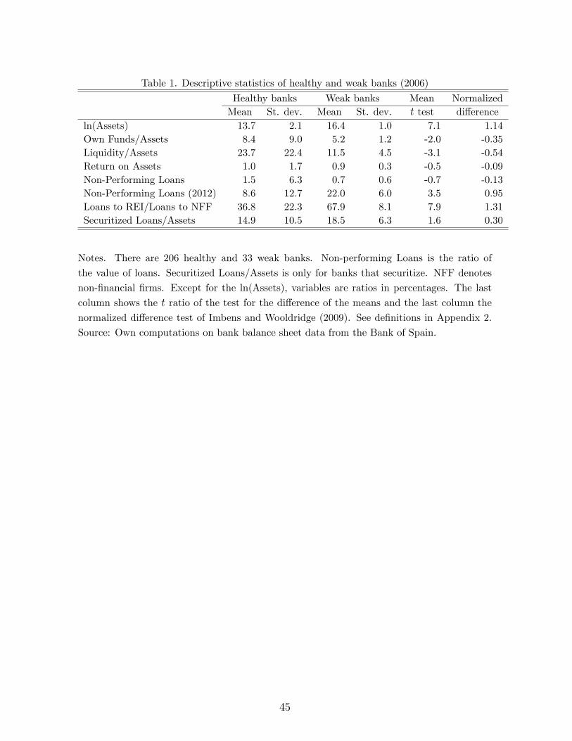
Table 1. Descriptive statistics of healthy and weak banks (2006)
Healthy banks Weak banks Mean NormalizedMean St. dev. Mean St. dev. t test di§erence
ln(Assets) 13.7 2.1 16.4 1.0 7.1 1.14Own Funds/Assets 8.4 9.0 5.2 1.2 -2.0 -0.35Liquidity/Assets 23.7 22.4 11.5 4.5 -3.1 -0.54Return on Assets 1.0 1.7 0.9 0.3 -0.5 -0.09Non-Performing Loans 1.5 6.3 0.7 0.6 -0.7 -0.13Non-Performing Loans (2012) 8.6 12.7 22.0 6.0 3.5 0.95Loans to REI/Loans to NFF 36.8 22.3 67.9 8.1 7.9 1.31Securitized Loans/Assets 14.9 10.5 18.5 6.3 1.6 0.30
Notes. There are 206 healthy and 33 weak banks. Non-performing Loans is the ratio of
the value of loans. Securitized Loans/Assets is only for banks that securitize. NFF denotes
non-Önancial Örms. Except for the ln(Assets), variables are ratios in percentages. The last
column shows the t ratio of the test for the di§erence of the means and the last column the
normalized di§erence test of Imbens and Wooldridge (2009). See deÖnitions in Appendix 2.
Source: Own computations on bank balance sheet data from the Bank of Spain.
45

Data: Six di§erent databases
1. Central Credit Register of the Bank of Spain (CIR):I All loans above e 6,000: identity of bank and borrower,collateral, maturity, etc.
I Firmsí credit history: non-performing loans and potentiallyproblematic loans
2. CIR (2): Loan applications by non-current borrowers
3. Annual balance sheets and income statements of Örms fromSpanish Mercantile Registers via SABI
I Exclude construction, real estate, and related industries:149,458 Örms
I Coverage: 19% Örms, 28% value added, 42% private employees
4. Firm entry and exit from Central Business Register
5. Bank balance sheets from supervisory Bank of Spain database
6. Bank location database
16 / 49

The treatment variable
I DeÖne: WB intensityi =Loans from weak banks
Asset value
= Weight of weak banks in debt # Leverage
I WBi = 1 if weak bank intensity >1st quartile (P25) ofdistribution of Örms with nonzero exposure in 2006 (4.8%)
I Excludes Örms with marginal attachment to weak banks fromthe treatment group
I Robustness: We also present results forI Other cuto§s: zero (any exposure), median (P50), and thirdquartile (P75)
I Continuous treatment: WB intensityi
17 / 49

Firm characteristics
I Full sample:I 98.7% SMEs (< 250 employees)I Employment in sample fell by 8.1% over 2006-2010I 31% had credit from weak banks, Avg. WB intensityi = 22.8%
I Treated Örms are on average:I Younger, smaller, more temporary workersI Finance: lower capital*, higher bank debt*, work with morebanks*, lower liquidity, less proÖtable, defaulted and appliedfor loans more often* = signiÖcant in normalized di§erence test of Imbens andWooldridge (2009)
18 / 49

I DX=(X1
-X0
)/q
S2
0
+ S2
1
versus
I t=(X1
-X0
)/q
S2
0
/N0
+ S2
1
/N1
where for w = 0, 1
S2
w
= Âi:Wi=w
(X$Xw)2/(Nw
$ 1)
the sample variance of Xi in the subsample with WI = w.
19 / 49

Table 2. Descriptive statistics of control and treated Örms (2006)
Control Treated Mean Norm.Mean St. Dev. P25 P50 P75 Mean St. Dev. P25 P50 P75 t test di§.
Loans with WB/Assets 0.3 0.9 0.0 0.0 0.0 22.8 17.1 9.7 17.3 30.9 427.3 1.31Share of Loans with WB 8.5 24.1 0.0 0.0 0.0 68.5 30.3 40.9 73.3 100.0 403.9 1.55Employment (employees) 25.3 365.6 2.0 6.0 13.0 20.3 207.2 2.0 5.0 13.0 -2.7 -0.01Temporary Employment 20.4 25.4 0.0 11.1 33.3 22.7 26.0 0.0 14.5 36.6 16.0 -0.06Age (years) 12.6 9.8 6.0 11.0 17.0 11.7 8.7 6.0 10.0 16.0 -17.1 -0.07Size (million euros) 5.8 118.2 0.3 0.6 1.7 3.6 27.5 0.3 0.6 1.7 -4.0 -0.02Exporter 13.0 33.7 0.0 0.0 0.0 13.1 33.7 0.0 0.0 0.0 0.3 0.00Own Funds/Assets 34.4 23.8 14.2 30.3 51.1 24.9 18.5 10.0 20.8 35.8 -74.3 -0.31Liquidity/Assets 12.4 15.1 1.9 7.0 17.4 8.6 11.8 1.1 4.2 11.2 -47.3 -0.20Return on Assets 6.7 11.4 1.8 4.9 10.2 5.2 9.0 2.0 4.4 8.0 -23.8 -0.10Bank Debt 30.7 26.7 6.8 24.8 49.8 48.5 23.5 29.4 47.4 66.2 120.8 0.50Short-Term Bank Debt (< 1 yr) 48.8 41.5 0.0 46.7 100.0 45.7 37.1 4.3 44.9 80.7 -13.2 -0.05Long-Term Bank Debt (> 5 yrs) 21.5 35.3 0.0 0.0 37.1 29.5 36.3 0.0 7.4 59.0 39.7 0.16Non-Collateralized Bank Debt 81.9 33.4 82.7 100.0 100.0 73.7 35.6 47.4 100.0 100.0 -42.3 -0.17Credit Line (has one) 69.0 46.3 0.0 100.0 100.0 72.2 44.8 0.0 100.0 100.0 12.5 0.05Banking Relationships (no.) 1.9 1.5 1.0 1.0 2.0 3.0 2.7 1.0 2.0 4.0 103.7 0.37Current Loan Defaults 0.3 5.6 0.0 0.0 0.0 0.6 7.4 0.0 0.0 0.0 6.8 0.03Past Loan Defaults 1.4 11.9 0.0 0.0 0.0 2.4 15.2 0.0 0.0 0.0 12.7 0.05Past Loan Applications 54.2 49.8 0.0 100.00 100.00 68.9 46.3 0.0 100.0 100.0 52.7 0.22All Loan Applications Accepted 22.0 41.4 0.0 0.0 0.0 26.2 44.0 0.0 0.0 100.0 17.6 0.07
Notes. Observations: 149,458 Örms; 106,128 control and 43,330 treated Örms. WB denotes weak banks. Variables are ratios inpercentages unless otherwise indicated. The twelfth column shows the t ratio on the test for the di§erence of the means and thelast column the normalized dißerence test of Imbens and Wooldridge (2009). See deÖnitions in Appendix 2.
46

Empirical strategy: 1. Credit supply shock
Di§erences in di§erences (DD) credit growth rate forÖrm-bank pairs:
Dt
log(1+ Creditib) = qi + pWBb + Z0ibk + S0bl+ eib
I Dt
= t-year di§erence (2006 to 2010), Creditib = creditcommitted by bank b to Örm i (drawn and undrawn), qi =Örm Öxed e§ect, WBb = 1 if bank b is a weak bank, Zib =Örm-bank controls (length of relationship, past defaults), Sb =bank controls. Note that log(1+ Creditib) keeps zeros
I Khwaja and Mian (2008): qi absorb any di§erences in Örmcharacteristics ! control perfectly for credit demand
I For Örms working with both types of banks, p tests whetherthe same Örm has a larger reduction in lending from weakbanks, controling for di§erences in Zib and Sb
20 / 49
Empirical strategy: 1. Credit supply shock
DD credit growth rate for (all) Örms:
Dt
log
"1+ Creditij
#= r+ µWBi +X0ih + dj + vij
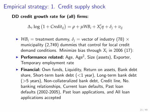
I WBi = treatment dummy, dj = vector of industry (78) #municipality (2,749) dummies that control for local creditdemand conditions. Minimize bias through Xi in 2006 (17):
I Performance related: Age, Age2, Size (assets), Exporter,Temporary employment rate
I Financial: Own funds, Liquidity, Return on assets, Bank debtshare, Short-term bank debt (<1 year), Long-term bank debt(>5 years), Non-collateralized bank debt, Credit line, No.banking relationships, Current loan defaults, Past loandefaults (2002-2005), Past loan applications, and All loanapplications accepted
21 / 49

Empirical strategy: 2. Employment e§ect
DD employment growth rate:
Dt
log
"1+ nij
#= a+ bWBi +X0ig+ dj + uij
I nij = employment in Örm i in industry#municipality cell j,typically from 2006 to 2010 ! Trends in all control variables
I nij set to zero for Örms in the sample in 2006 but not in 2010because they closed down ! log(1+ nijkt) ! Surviving andclosing Örms
Ib measures Average Treatment e§ect on the Treated (ATT)
22 / 49

Credit supply shock: Örm-bank
Dependent variable: D4
log(1+ Creditib)
Multi-bank Fixed Credit Positive REIÖrms e§ects lines credit expos.
WBb -0.256&&&
-0.255&&&
-0.079&&
-0.180&
(0.094) (0.008) (0.034) (0.096)Credit line 0.074
&&&
(0.015)Credit line -0.106
&&&
# WBb (0.039)
R2 0.059 0.407 0.452 0.394 0.406No. Örms 72,287 72,287 72,286 42,630 72,287No. obs. 236,691 236,691 236,689 126,863 236,691
23 / 49

Credit supply shock: Örm-bank
I Multi-bank " Fixed e§ects: unobservables not very importantI Hausman test fails to reject the null hypothesis oforthogonality between the Örm Öxed e§ects and WBb (p-value= 0.372) ! WBb captures changes in credit supply
I WBs reduced credit to Örms with credit lines by 10.6 pprelative to other banks ! suggests an e§ect on workingcapital rather than investment
I Reductions in lending to continuing borrowers accounts forsmall share of reduction in lending by WBs
I Exposure to REI: share of bankís loans to Örms in the REI in2006 in the upper quartile of the distribution: 10 pp lowere§ect than WB dummy
24 / 49

Credit supply shock: Örm level
Dependent variable: D4
log(1+ Creditij)
All Multi- RealÖrms bank estate
WBi -0.053&&&
-0.031&&&
-0.039&&&
(0.015) (0.011) (0.017)
R2 0.215 0.246 0.215No. obs. 149,458 74,045 149,458
Firm controls, industry#municipality Öxed e§ects, and Örm controls
25 / 49

Credit supply shock: Örm level
I E§ect at the Örm level is about one-Öfth of the size of thee§ect at the Örm-bank level: Treated Örms managed to o§seta substantial part of the reduction in credit but not all ( 6=JimÈnez et al., 2014, for Spain in the expansion)
I A pre-crisis banking relationship with more than one bankprovided some insurance against the shocks that hit WBsduring the crisis ( 6= Gobbi and Sette, 2014, for Italy duringthe Great Recession)
I Magnitude: attachment to weak banks explains about 34% ofthe di§erential fall in credit for attached Örms
26 / 49

Employment e§ects: baseline
Dependent variable: D4
log
"1+ nij
#
No Örm SigniÖcantly Baseline Main Placebocontrols di§. controls bank f.e. í02-í06
WBi -0.076&&&
-0.035&&&
-0.028&&&
-0.028&&&
0.006(0.013) (0.006) (0.006) (0.006) (0.007)
R2 0.046 0.163 0.155 0.179 0.203No. obs. 149,458 149,458 149,458 149,458 112,933
Industry#municipality Öxed e§ects included
27 / 49

Employment e§ects: baseline
I Large change in e§ect due to including signiÖcantly di§erentcontrol variables across treated and control Örms, not fromincluding remaining controls
I Controling for main bank Öxed e§ects does not alter theresults ! WB indicator captures the relevant dimensions thatexplain reduced access to credit for treated Örms
I Placebo test: 2002 as the pre-crisis year and 2006 as thepost-crisis year ! coe¢cient not signiÖcantly di§erent fromzero
I Year by year e§ects: start being signiÖcant in 2008 (Ögure)
28 / 49

Employmenteffects:baseline��Impactofweak-bankaLachmentonemployment
with95%confidencebands(%)

Employment e§ects: transmission
IV model for employment growth rate:
Dt
log
"1+ nij
#= s+ fD
t
log
"1+ Creditij
#+X0ix + dj + #ij
Dt
log
"1+ Creditij
#= r+ µWBi +X0ih + dj + vij
I WBi is an instrument for access to credit, Örst stage coincideswith the previous Örm-level credit equation, µf is equivalentto b in baseline equation
I Exclusion restriction: working with a weak bank altersemployment growth only through credit
I Decomposition: Credit-volume e§ect of WBi # E§ect ofpredicted credit volume on employment
30 / 49

Employment e§ects: transmission
Dependent variable: D4
log
"1+ nij
#
All Örms Multi-bank ÖrmsInstrumented variable D
4
log(1+Creditij)0.519
&&&0.797
&&&
(0.179) (0.294)First stage
WBi -0.053&&&
-0.031&&&
(0.015) (0.011)
Overall e§ect -0.028 -0.025
F test / p value 13.1/0.00 7.65/0.00No. obs. 149,458 74,045
Firm controls and industry#municipality Öxed e§ects included
31 / 49
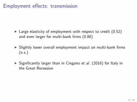
Employment e§ects: transmission
I Large elasticity of employment with respect to credit (0.52)and even larger for multi-bank Örms (0.80)
I Slightly lower overall employment impact on multi-bank Örms(n.s.)
I SigniÖcantly larger than in Cingano et al. (2016) for Italy inthe Great Recession
32 / 49
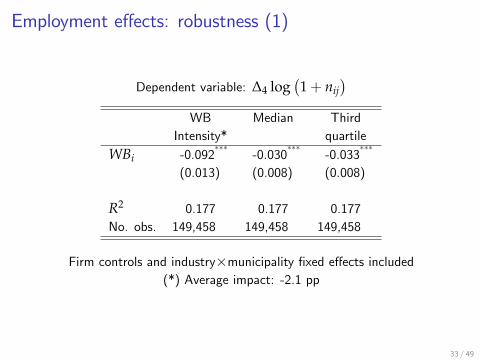
Employment e§ects: robustness (1)
Dependent variable: D4
log
"1+ nij
#
WB Median ThirdIntensity* quartile
WBi -0.092&&&
-0.030&&&
-0.033&&&
(0.013) (0.008) (0.008)
R2 0.177 0.177 0.177No. obs. 149,458 149,458 149,458
Firm controls and industry#municipality Öxed e§ects included(*) Average impact: -2.1 pp
33 / 49

Employment e§ects: robustness (2)
Dependent variable: D4
log
"1+ nij
#
Survivors Alternat. Tradable Loansmeasure* goods to REI
WBi -0.014&&&
-0.034&&&
-0.058&&&
-0.030&&&
(0.004) (0.004) (0.023) (0.008)
R2 0.181 0.183 0.200 0.177No. obs. 133,122 149,458 16,199 149,458
Firm controls and industry#municipality Öxed e§ects included(*) Dnij = (nijt $ nijt$1
)/(0.5(nijt + nijt$1
))
34 / 49
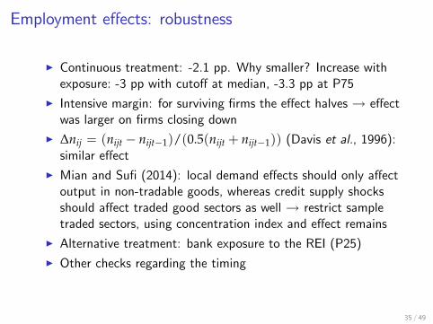
Employment e§ects: robustness
I Continuous treatment: -2.1 pp. Why smaller? Increase withexposure: -3 pp with cuto§ at median, -3.3 pp at P75
I Intensive margin: for surviving Örms the e§ect halves ! e§ectwas larger on Örms closing down
I Dnij = (nijt $ nijt$1
)/(0.5(nijt + nijt$1
)) (Davis et al., 1996):similar e§ect
I Mian and SuÖ (2014): local demand e§ects should only a§ectoutput in non-tradable goods, whereas credit supply shocksshould a§ect traded good sectors as well ! restrict sampletraded sectors, using concentration index and e§ect remains
I Alternative treatment: bank exposure to the REI (P25)I Other checks regarding the timing
35 / 49

Selection
I Lower bound: Oster (2015). If R2 increases when controls areincluded but coe¢cient does not vary much ! inclusion ofunobservables would not alter it much either. With heuristicassumption that R
max
= 1.3
eR, where eR is the fully-controlledR2 and R
max
is the maximum R2 that would be obtained if allpotential determinants were included. Estimate on WB = -1.1pp (lower bound)
I Panel with Örm Öxed e§ects: Same e§ect by 2010 as baseline
37 / 49
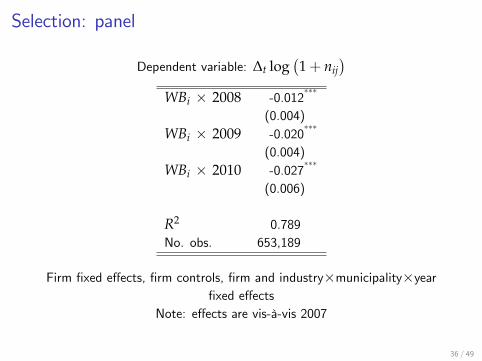
Selection: panel
Dependent variable: Dt log
"1+ nij
#
WBi # 2008 -0.012&&&
(0.004)WBi # 2009 -0.020
&&&
(0.004)WBi # 2010 -0.027
&&&
(0.006)
R2 0.789No. obs. 653,189
Firm Öxed e§ects, Örm controls, Örm and industry#municipality#yearÖxed e§ects
Note: e§ects are vis-‡-vis 2007
36 / 49

Selection: matching
Dependent variable: D4
log
"1+ nij
#
Propensity Exact Propensity Exactscore score
WBi -0.032&&&
-0.026&&&
(0.009) (0.006)WBi intensity -0.065
&&&-0.052
&&&
(0.024) (0.021)
Overall e§ect ñ ñ -0.015 -0.012
R2 0.228 0.179 0.228 0.245No. obs. 43,587 133,816 16,199 133,816
Firm controls and industry#municipality Öxed e§ects included
38 / 49

Selection: matching
I Propensity score: (1) probit model for the probability that aÖrm borrows from a WB, and (2) estimate baseline modelusing weights from the sample balanced on observables usedfor the p-score
I Exact matching: treated and non-treated Örms within cellsdeÖned by: industry # municipality and Örm controls.Coarsened exact matching method (Iacus et al., 2011):variables entered as 0-1 dummy variables, treatment e§ect isestimated using WLS
I Post-matching balance tables for both methods show no traceof signiÖcant di§erences in control variables across treatedand control Örms according to normalized di§erence test
I Propensity score matching delivers larger e§ects and, asbefore, continuous measure implies lower efects
39 / 49

Selection: exogenous exposure
I Until 1988 savings banks could only open 12 branches outsidetheir region of origin, at the end of December 1988restrictions were lifted
I IV for WBi in 2006: WB density by municipality, i.e. share ofbank branches in December 1988 belonging to WBs(traditional strong market position)
I Exclusion restriction: local WB density only a§ects a Örmísemployment through its attachment to WBs
I Indirect evidence: Örms in municipalities with local WBdensity above the median very similar to Örms below themedian in all respects, balance tables show no signiÖcantdi§erence
I Problem: estimates potentially include local generalequilibrium e§ects from having WBs ! untestable
40 / 49

Selection: exogenous exposure
Dependent variable: D4
log
"1+ nij
#
Instrumented variable WBi WBiintensity
-0.076&&&
-0.320&&&
(0.036) (0.157)First stage
Weak bank density 0.445&&&
0.105&&&
(0.084) (0.025)
Overall e§ect -0.076 -0.073
F test / p value 17.8/0.00 28.3/0.00No. obs. 149,458 149,458
Firm controls and industry and coast Öxed e§ects included
41 / 49

Financial vulnerability (DDD)
Dependent variable: D4
log(1+ nij)
Rejected applicationsi -0.066&&&
log(Total Assets)i 0.009&
(0.008) (0.003)Rejected applic.i#WBi -0.029
&&log(Total Assets)i#WBi 0.003
(0.012) (0.005)Defaultsi -0.209
&&&Single banki 0.012
&&
(0.029) (0.007)Defaultsi#WBi -0.041
&&Single banki#WBi 0.019
(0.020) (0.015)Short-term debti -0.089
&&& WBi -0.019&&&
(0.013) (0.007)Short-term debti#WBi -0.036
&&& R2 0.176(0.017) No. obs. 149,458
Firm controls and industry#municipality Öxed e§ects, and levels andinteractions of WBi with own funds, liquidity, age, exporter, temporary
employment, and broad industry42 / 49

Financial vulnerability (DDD)
I Large e§ects on employment of bad credit history andshort-term debt
I No e§ect of size: results in literature may be due to lack ofcontrol for creditworthiness
I No e§ect of single bank (consistent with our previous result)
43 / 49

Margins of adjustment in surviving Örms
Dependent variable D4
"ntemp,ij/nij
#D
4
log
"Wage billij
#
WBi -0.005&&&
-0.016&&&
(0.002) (0.006)
R2 0.174 0.205No. obs. 122,725 87,451
Firm controls and industry#municipality Öxed e§ects included
44 / 49

Margins of adjustment in surviving Örms
Temporary employment
I Type of contract observed for 91% of surviving Örms: tempemployment share fell by -0.5 pp due to WB attachment
I WB attachment caused 1.4 pp drop in total employment,initial temp share = 21% ! drop in temporary employment =3.7 pp ! 56% of employment adjustment in treated Örms
Wage bill
I WB attachment caused -1.6 pp (v non-attached Örms),employment e§ect = -1.4 pp ! average wage fell by 0.2 pp
I It could be driven by composition e§ects (workercharacteristics), but it suggests that wage adjustments did notplay a meaningful role to mitigate credit supply shock
45 / 49

Probability of exit
Dependent variable: Probability of exit from 2006 to 2010i
WBi 0.011&&&
(0.004)WB Intensityi 0.059
&&&
(0.014)
R2 0.173 0.173No. obs. 150,442 150.442
Firm controls and industry#municipality Öxed e§ects included
I WB: 1.1 pp " 10.8% increase w.r.t. baseline exit (10.2%)
I WB Intensityi: 9th v. 1st decile ! 1.5% higher probability "14.5% w.r.t baseline exit rate
46 / 49

Job loss estimates
Caveat: These are not macro e§ects (Chodorow-Reich, 2014), onlydi§erential e§ects
Aggregate job losses in exposed Örms due to WB attachment:
I Baseline: 24.4% of job losses at exposed Örms! 7% of overall job losses
I With separate estimates: Survivors: 48%; closing Örms: 52%of job losses
47 / 49

Conclusions
I Aim: measure the impact of credit constraints on employmentduring the Great Recession in Spain
I IdentiÖcation: We exploit di§erences in lender health at theonset of the crisis, as evidenced by savings banksí bailouts
I We Önd that job losses from expansion to recession at Örmsexposed to weak banks are signiÖcantly larger than at similarnon-exposed Örms
I This explains around one-fourth of aggregate job losses atexposed Örms
48 / 49
Conclusions
I The estimated e§ects vary considerably with the Örmís size,creditworthiness and the structure of its banking relationships
I Brunt of the adjustment was borne by temporary workers,with little adjustment in wages
I Credit constraints do not just force Örms to purge jobs butalso cause some of them to close down
I Given our controls, constrained Örms would have receivedmore credit had they not been attached to weak banks and, Inthis sense, while some part of job losses su§ered by Örmsattached to weak banks was probably e¢cient, the estimatedemployment e§ects of the credit constraints we identify, onceselection has been taken into account, were ine¢cient.
49 / 49