creating multi objective value functions from non
TRANSCRIPT

Air Force Institute of Technology Air Force Institute of Technology
AFIT Scholar AFIT Scholar
Theses and Dissertations Student Graduate Works
3-9-2009
Creating Multi Objective Value Functions from Non-Independent Creating Multi Objective Value Functions from Non-Independent
Values Values
Christopher D. Richards
Follow this and additional works at: https://scholar.afit.edu/etd
Part of the Other Mathematics Commons, and the Statistical Models Commons
Recommended Citation Recommended Citation Richards, Christopher D., "Creating Multi Objective Value Functions from Non-Independent Values" (2009). Theses and Dissertations. 2618. https://scholar.afit.edu/etd/2618
This Thesis is brought to you for free and open access by the Student Graduate Works at AFIT Scholar. It has been accepted for inclusion in Theses and Dissertations by an authorized administrator of AFIT Scholar. For more information, please contact [email protected].

CREATING MULTI OBJECTIVE
VALUE FUNCTIONS FROM
NON-INDEPENDENT VALUES
Christopher D. Richards, Captain, USAF
AFIT/GOR/ENS/09-12
DEPARTMENT OF THE AIR FORCE AIR UNIVERSITY
AIR FORCE INSTITUTE OF TECHNOLOGY
Wright-Patterson Air Force Base, Ohio
APPROVED FOR PUBLIC RELEASE; DISTRIBUTION UNLIMITED.

The views expressed in this thesis are those of the author and do not reflect the official policy or position of the United States Air Force, Department of Defense, or the United States Government.

AFIT/GOR/ENS/09-12
CREATING MULTI OBJECTIVE VALUE FUNCTIONS FROM
NON-INDEPENDENT VALUES
THESIS
Presented to the Faculty
Department of Operational Sciences
Graduate School of Engineering and Management
Air Force Institute of Technology
Air University
Air Education and Training Command
In Partial Fulfillment of the Requirements for the
Degree of Master of Science in Operations Research
Christopher D. Richards, BS
Captain, USAF
March 2009
APPROVED FOR PUBLIC RELEASE; DISTRIBUTION UNLIMITED.

AFIT/GOR/ENS/09-12
Creating Multi Objective
Value Functions From
Non-Independent Values
Christopher D Richards, BS Captain, USAF
Approved: ____________________________________ ___ Dr. Jeffery D. Weir (Co-Chairman) date ____________________________________ ___ Shane Knighton, Maj, USAF (Co-Chairman) date

iv
AFIT/GOR/ENS/09-12
Abstract
Decisions are made every day and by everyone. As these decisions become
more important, involve higher costs and affect a broader group of stakeholders it
becomes essential to establish a more rigorous strategy than simply intuition or “going
with your gut”. In the past several decades, the concept of Value Focused Thinking
(VFT) has gained much acclaim in assisting Decision Makers (DMs) in this very effort. By
identifying and organizing what a DM values VFT is able to decompose the original
problem and create a mathematical model to score and rank alternatives to be chosen.
But what if the decision should not be completely decomposed? What if there are
factors that are inextricably linked rather than independent? In the past several years,
Improvised Explosive Devices (IEDs) have quickly become the number one killer of
American troops overseas. To this end the Joint IED Defeat Organization worked to
create a VFT model to solicit and grade countermeasure proposals as candidates for
funding. While much time and care was put into soliciting a valid VFT hierarchy from
the appropriate DM, it does not represent the only option. With JIEDDO as an example
this paper examines a strategy to better reflect a DM’s combined values in a way which
is understandable to the DM and maintains a level of mathematical rigor.

v
AFIT/GOR/ENS/09-12
Dedication
To my Wife, without whom this paper would be no more than the ramblings of a crazy person with screaming children.

vi
Acknowledgments
Deep thanks are in order for all those who indulged me in my incessant research
and questioning; specifically the patience of Maj Shane Knighton for taking the time to
make decision analysis something tangible rather than equations in a book and to LtCol
Jeffery Weir who did not hesitate jumping to my aid when I most needed it. Also, to
those deployed members of the Marines and Army who helped me better understand
the complexity of the threat posed by IEDs, thank you.
Chris D. Richards

vii
Table of Contents
Abstract ............................................................................................................................... iv
Dedication ............................................................................................................................ v
Acknowledgments............................................................................................................... vi
Index of Tables: .................................................................................................................... x
Index of Figures: ................................................................................................................... x
I. Introduction ................................................................................................................. 1
I.A Background ................................................................................................................ 3
I.B Problem Statement .................................................................................................... 5
I.C Thesis Objective ......................................................................................................... 5
I. D Methodology / Limitations ....................................................................................... 6
I.E Paper Organization .................................................................................................... 7
II. Literature Review ........................................................................................................ 8
II.A Decision Analysis....................................................................................................... 8
II.B Value Focused v. Alternative Focused ...................................................................... 9
II.C Measure Selection and Construction ..................................................................... 10
II.D Additive Value Functions and Preferential Independence .................................... 11
II.E Multiplicative Functions .......................................................................................... 14
II.F Multilinear Functions .............................................................................................. 16
II.G Constructed Scales ................................................................................................. 17
II.H Hidden Objectives .................................................................................................. 18
II.I General Regression .................................................................................................. 19
III. Methodology .......................................................................................................... 21
III.A Requirements ..................................................................................................... 21
III.B Assumptions ....................................................................................................... 22
III.C Solicitation .......................................................................................................... 24
III.D Processing ........................................................................................................... 31
IV. Results & Analysis .................................................................................................. 38
IV.A Overview ................................................................................................................ 38
IV.B Measure Creation .................................................................................................. 38

viii
IV.C Value Function Comparison .................................................................................. 43
IV.D Alternative Scoring & Ranking............................................................................... 45
IV.E Rank Testing ........................................................................................................... 49
IV.F Sensitivity Analysis ................................................................................................. 52
IV.F Marine Model and Additional Findings ................................................................. 54
V. Conclusions and Recommendations ......................................................................... 58
V.A Research Review ..................................................................................................... 58
V.B Contributions .......................................................................................................... 59
V.C Future Research ...................................................................................................... 60
V.D Summary ................................................................................................................ 62
Appendix A ........................................................................................................................ 63
A.1: Directly Solicited Value Matrices (Researcher) ..................................................... 63
A.2: Directly Solicited Value Matrices (Marine Commander) ...................................... 64
A.3: Mathematically Interpolated Value Matrices (Researcher) .................................. 65
A.4: Mathematically Interpolated Value Matrix (Marine Commander) ....................... 66
Appendix B ........................................................................................................................ 67
B.1: Alternative Factor Levels ...................................................................................... 67
B.2: Factor Scoring ....................................................................................................... 68
Appendix C ........................................................................................................................ 69
C.1: Concordance Calculations (Researcher) ............................................................... 69
C.2 Concordance Calculations (Marine Commander): ................................................. 70
Appendix D: ....................................................................................................................... 71
D.1: Group Rankings (5 Alternative / n=6) - Researcher.............................................. 71
D.2: Group Rankings (5 Alternatives / n=6) – Marine Commander ............................. 72
D.3: Group Rankings (3 Alternatives / n=10) ............................................................... 73
D.4: Group Rankings (3 Alternatives / n=10) – Marine Commander ........................... 74
Appendix E ........................................................................................................................ 75
E.1: Matrix Representation of Independent Value Pairs ............................................. 75
Appendix F ........................................................................................................................ 76
F.1: Sensitivity Analysis (Needed Capability) ............................................................... 76
F.2: Sensitivity Analysis (Operational Performance).................................................... 77
F.3: Sensitivity Analysis (Usability) ............................................................................... 78

ix
Appendix G ........................................................................................................................ 79
”All Models Are Wrong…” ............................................................................................. 79
Bibliography ...................................................................................................................... 82
Vita .................................................................................................................................... 88

x
Index of Tables: TABLE 1: CATEGORICAL VALUES ............................................................................................................. 28 TABLE 2: CONTINUOUS BREAK VALUES ................................................................................................................. 28 TABLE 3: ADJUSTED VALUES ............................................................................................................................... 29 TABLE 4: CATEGORICAL VALUES .................................................................................................................... 30 TABLE 5: UPDATED CONTINUOUS W/ MIDVALUES .................................................................................................. 31 TABLE 6: TWO-DIMENSIONAL VALUE MATRIX ........................................................................................................ 31 TABLE 7: VALUE MATRIX.................................................................................................................................... 33 TABLE 8: MATRIX W/ CALCULATED VALUES ........................................................................................................... 34 TABLE 9: TWO-WAY INTERPOLATION .................................................................................................................... 35 TABLE 10: TWO-DIMENSIONAL VALUE MATRIX ...................................................................................................... 37 TABLE 11: GAP GIVEN TIME TO COUNTER .............................................................................................. 41 TABLE 12: TIME TO COUNTER GIVEN GAP ........................................................................................................ 42 TABLE 13: TRL GIVEN MONTHS TO FIELDING ............................................................................................ 41 TABLE 14: MONTHS TO FIELDING GIVEN TRL .................................................................................................... 42 TABLE 15: TRAINING TIME GIVEN MATURITY ............................................................................................ 42 TABLE 16: MATURITY GIVEN TRAINING TIME .................................................................................................... 42 TABLE 17: COMPLETE SOLICITATION OF PRIMARY GAP & TIME TO COUNTER ................................................................ 43 TABLE 18: INDEPENDENT VALUE CALCULATION ...................................................................................................... 43 TABLE 19: JIEDDO ALTERNATIVE SCORES ............................................................................................................. 47 TABLE 20: JIEDDO ALTERNATIVE RANKINGS ......................................................................................................... 48 TABLE 21: GROUP RANKING COMPARISONS .......................................................................................................... 52
Index of Figures: FIGURE 1: A JIEDDO VFT HIERARCHY .................................................................................................................... 4 FIGURE 2: INDIVIDUAL SDVF’S ............................................................................................................................ 11 FIGURE 3: POWER ADDITIVE MODEL ..................................................................................................................... 15 FIGURE 4: ALLOWED INTERACTIONS ...................................................................................................................... 23 FIGURE 5: IDENTIFIED INTERACTIONS ..................................................................................................................... 26 FIGURE 6: BREAKPOINTS ..................................................................................................................................... 27 FIGURE 7: PIECEWISE LINEAR V. EXPONENTIAL W/ RHO=0.1 ...................................................................................... 30 FIGURE 8: INTERACTIONS ................................................................................................................................... 39 FIGURE 9: INDEPENDENT ADDITIVE VALUE FUNCTION (VALUE V. TIME TO COUNTER) .................................................... 44 FIGURE 10: DIRECTLY SOLICITED COMBINED VALUE FUNCTIONS (VALUE V. TIME TO COUNTER) ...................................... 45 FIGURE 11: INTERPOLATED COMBINED VALUE FUNCTIONS (VALUE V. TIME TO COUNTER) ............................................. 45 FIGURE 12: NEEDED CAPABILITY SENSITIVITY ANALYSIS (ORIGINAL MODEL) ................................................................ 53 FIGURE 13: NEEDED CAPABILITY SENSITIVITY ANALYSIS (COMPLETE SOLICITATION) ....................................................... 53 FIGURE 14: MARINE MODEL ALTERNATIVE RANKING .............................................................................................. 55 FIGURE 15: DIRECTLY SOLICITED VALUES .............................................................................................................. 56 FIGURE 16: PARTIALLY SOLICITED VALUES W/ INTERPOLATION .................................................................................. 56
1
CREATING MULTI OBJECTIVE
VALUE FUNCTIONS FROM
NON-INDEPENDENT VALUES
I. Introduction
One of the primary applications of DA has been in initiative selection. Individuals,
companies and especially militaries are consistently faced with some sort of ambiguous
objective (raise profits, lower costs, defeat the enemy) and must decide which initiatives
can be started now which will have the greatest likelihood of accomplishing these goals
in the future. In 1998 the Chief of Staff of the US Air Force was faced with just such a
situation: What space and air systems should we start now in order to guarantee air
and space dominance in 2025? The resultant study by Air University attacked the
problem using a classic additive VFT model that graded 40+ notional futuristic systems
(in six notional futures) on their ability to support such the desired superiority (Parnell,
Conley, Jackson, Lehmkuhl, & Andrew, 1998).
Unsurprisingly the actual DM (in this case Gen Fogleman) was largely unavailable for
interview during the study. As a result, researchers were forced to revert to what
Kirkwood refers to as the “gold” and “silver” standards of information; official doctrine
and the opinions of subject matter experts (SME) (Kirkwood, 1997). In the end, the
study relied almost completely on SME’s rather than the gold standard of doctrine due
to the fact that, as they explained “It provides a high-level strategic view of national

2
defense policy but does not provide detailed objectives for a value hierarchy” (Parnell,
Conley, Jackson, Lehmkuhl, & Andrew, 1998).
Much like the current JIEDDO model, AF 2025 was a step in the right direction but
arguably lost valuable insight into ranking initiatives by ignoring “the bigger picture”.
The “high-level” view that the policy offered could very well have provided a holistic
view of alternatives, allowed at least some level of interaction within measures, and
have better modeled the effects of future air and space systems. In AFDD 1, Air Force
Basic Doctrine, General Jumper clearly states that “… the complex integration required
among our fighting elements, the complexity of joint and combined doctrine, and the
uncertainty of rapidly developing contingency operations demand that our planning and
employment be understood and repeatable” (United States Air Force, 2003). General
Jumper’s choice of words such as complex, integration and joint all point to a clear
recognition that some decisions have at their core, values which are not necessarily
simple or the result of only one attribute. This does not mean that these values are
impossible to ascertain and quantify.
This thesis proposes strategies for expanding a VFT model to more realistically
reflect the combined values and tradeoffs of military leaders. This section specifically
looks at a model currently designed for JIEDDO and introduces a framework for
improvement.

3
I.A Background
Due to the growing threat that IEDs posed to soldiers in both Iraq and Afghanistan,
in 2003 the US Army created the IED Task Force in order to explore countermeasures.
Amid early success it quickly became apparent that the high level of reach out to sister
services and interaction was indicative of an initiative which would benefit from
attention at the DoD level and not only the Army. As a result, in 2006 DODD 200019.E
replaced the task force with JIEDDO (JIEDDO, 2008) as a permanent military body.
JIEDDO is charged to “… focus (lead, advocate, coordinate) all Department of Defense
actions in support of the Combatant Commanders’ and their respective Joint Task
Forces’ efforts to defeat Improvised Explosive Devices as weapons of strategic
influence.” Systems to further this goal are divided between defeating the IED (e.g.
mitigating effects through armor or disposal), defeating the system (interrupting the
chain of IED activities) and training the force (through doctrine, technology, etc.)
(Department of Defense, 2006). To that end, JIEDDO solicits proposals for approval and
funding through the Joint IED Defeat Capability Approval and Acquisition Management
Process. In appropriating such a budget (almost $2B in 2007) (Meigs, 2007) officials,
both commercial and governmental, require a high-level of justification and
transparency for decisions before any funds can be committed (Government
Accountability Office, 2008).
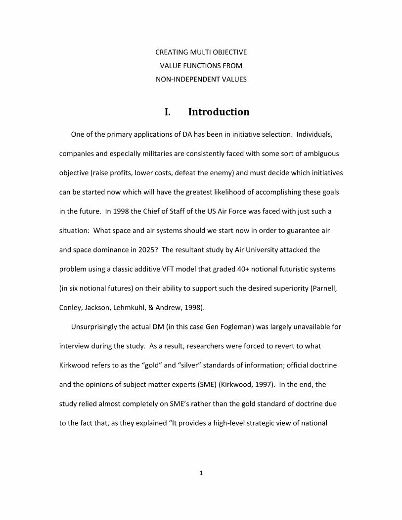
In 2008 Dawley et al. suggested a VFT model for JIEDDO proposal selection. Key
JIEDDO decision makers (DMs) as well as other personnel were interviewed and

4
questioned on what aspects were most important to potential IED countermeasures and
what measures best reflected these values (Dawley, Lenore, & Long, 2008).
Figure 1: A JIEDDO VFT Hierarchy
As with most value models, there are two immediate advantages to this hierarchy:
1) It defines the “ideal” IED defeat solution. By identifying all desired
characteristics and their relative importance, JIEDDO greatly reduces the
probability of finding themselves in a situation where they are forced to choose
the “best of the worst” from a list of submitted proposals. Instead, proposals are
able to be shaped directly by specific JIEDDO requirements.
2) Once defined and weighted, the single dimensional value functions (SDVF) which
govern the measures can easily be summed to give an overall “score” or value
for a particular alternative allowing it to be ranked against others competing for
selection.
Potential to
Defeat IED
1.00
Needed
Capability
.400
Operational
Performance
.350
Usability
.250
Gap Impact
.176
Classification
.056
Time to
Counter
.112
Technical
Performance
.110
Suitability
.056
Interoperability
.091
Technical Risk
.037
Fielding
Timeline
.056
Operations
Burden
.087
Work Load
.100
Required
Training
.063
Training
Time
.050
Program
Maturity
.013
# Tenets
Impacted
Primary Gap
Addressed
Classification
Level
Months Useful
Operation
Performance
Rating
Suitability
Rating
Interoperability
Issues
Technology
Readiness
Level
Months to
Fielding
% Maximum
Capacity
Interaction
Minutes per
Hour
Training Hours
Required
Training Level
Tenets
Impacted
.056

5
As we will discuss later, Kirkwood lays out several desirable properties for a value
hierarchy (Kirkwood, 1997). Among these, completeness, non-redundancy, operability
and small size all seem to be relatively satisfied by the hierarchy in Figure 1 and support
the definition of an ideal solution. Decomposability however, is more complicated.
While the decomposition of a complex value may offer sub-values that are simpler to
score, this substitution may lose important insight into why the original value was
important to the DM.
I.B Problem Statement
The current JIEDDO model claims independence assumptions about values based
on DM input. While these assumptions allow for a simple scoring structure and require
a minimum of DM input, they may lose important information about interactions and
lead to alternatives that may be holistically preferred by a DM to be outranked by
alternatives which score well only on individual objectives. How does one create a value
model which captures interactions without an unduly lengthy DM solicitation?
I.C Thesis Objective The objective of this thesis is to introduce an alternate strategy for the analyst to
employ during value model solicitation if they or the DM suspect that there exists
preferential dependence between one or more values. The hope is to build on the
prescribed VFT methodology leaving a process that is clear to a DM with little to no
extra explanation as well as maintaining the mathematical foundation which makes the
additive model such a desirable and defendable template.

6
I. D Methodology / Limitations
Although the original JIEDDO VFT model was created over a year ago, it has yet
to be implemented by its organization. During this time JIEDDO has continued to
receive, evaluate and decide to either accept or reject hundreds of proposals; the
current model is understood but not completely accepted. The task will be to use the
current VFT model as a foundation for an improved model which can lay to rest to any
fears or suspicions of preferential dependence with minimal additional time
requirements on the DM. This method should be DM independent and should answer
the question of dependence without assuming its existence.
There are two major limitations in this effort: First, while there exists a large
archive of accepted and rejected JIEDDO proposals, they have not been scored through
the current VFT model. With minimal access to SME’s, this task falls upon the
researcher and is complicated not only by the number of proposals and measures to be
scored, but also due to unclear definitions of desired performance levels. As a result,
analysis depends greatly on the previous alternative scoring accomplished by Dawley's
team in 2008. The second limitation is access to the relevant DM. Due to the
continuous and high-vis nature of JIEDDO, meetings with actual DMs have been short
and small in number. To fill this shortfall potential numbers are developed in order to
provide an illustrative example as proof of concept of the methodology for future
meetings.

7
I.E Paper Organization
The remainder of this paper is divided into four chapters: Chapter two presents
a brief background of decision analysis as well as currently available alternatives for
addressing the issue of dependence within value models. Chapter three introduces a
new method for handling these issues and proscribes a step-by-step method for its
execution with a decision maker. In Chapter four deterministic and sensitivity analysis
are applied to the results of the newly established methodology as applied to the
JIEDDO model using a sample set of past proposals submitted to the organization.
Finally, conclusions as to the value of the presented model as well as recommendations
for future research surrounding the topic are offered in Chapter five.

8
II. Literature Review
II.A Decision Analysis
Whether they realize it or not almost everyone practices some level of decision
analysis (DA) every day. Kirkwood argues that any time we are faced with several
alternatives which cannot all be chosen and have different consequences, then we are
faced with a decision (Kirkwood, 1997). While decisions can range from relatively
insignificant (where to go to lunch today?) to life or death (should I launch a nuclear
attack?) DA provides a framework for methodically quantifying what is important to the
decision maker (DM) and helping to choose the alternative which best accomplishes the
overall goals of the DM. After identifying the driving objective, DA works to break the
objective into its constituent pieces until they are at a level which is measurable either
directly or indirectly. Returning to the question of where to go to lunch, the objective
may be to “Eat Lunch” which can be broken down into “Proximity”, “Cost”, and
“Tastiness”. The first two can be measured directly by miles and dollars while the last
could be based on some constructed scale of past experience. While it is completely
plausible that the DM may end up making the same decision that they would have had
they simply “gone with their gut”, the decomposition has several key advantages. First,
it helps the DM to organize their thoughts in making a decision. Second, it allows for
transparency and justification of the decision process to others (Why are we going to
lunch here? Because the other restaurant may be closer but this one is half the price
and twice as good.) Finally, after a decision is made, it can serve to either help figure

9
out where things went wrong (20 miles is too far for lunch) or identify important
elements of success (Tastiness is definitely more important than cost).
II.B Value Focused v. Alternative Focused
There are two main camps between which DA techniques divide: the Analytical
Hierarchy Process (AHP) and the aforementioned VFT. Developed by Saaty, AHP
assumes a list of alternatives already exists and builds measures for scoring the
alternatives by assessing a DM’s preference between alternatives on particular
measures (Given these two cars, which rates higher on dependability?) (Saaty, 1986).
While many have argued that AHP suffers from practical problems and inconsistencies
which make it undesirable for many DMs (Dyer, 1990), it does help in “…deriving
dominance priorities from paired comparisons … with respect to a common criterion”
(Saaty, 1994) and may help to prove broader concepts then just making a decision
according to Kirkwood (Kirkwood, 1997).
VFT on the other hand attempts to break free of the box to which AHP is
confined by developing objectives and measures free of pre-existing alternatives. In
practice this forces a DM to consider what is really important to them instead of simply
choosing the best of what’s available. At its best VFT helps to guide the alternative
generation process and innovate new ideas, at its worst it results in a framework for
choosing between alternatives and is generally no less effective than AHP. According to
Kirkwood “There is no substitute for a good alternative.” (Kirkwood, 1997)

10
While AHP and VFT seek to create objectives and measures differently, they both
result in a hierarchy that is used to measure each alternative on a set of individual
measures that are then aggregated into a single score that is used to rank overall
preference of alternatives
II.C Measure Selection and Construction Up to this point DA has been described basically as a decomposition of the
decision problem into measurable pieces in an attempt to make the analysis more
manageable. However, measures are useless without clear definition.
Looking back at our lunch example in II.A, consider the sub-objective of
Proximity. While distance seems to be the obvious choice, we could just as easily use
time if we know that traffic is an issue. Further, even if distance is chosen, to be
complete we may need to define how distance is measured (strict Euclidean distances
are rarely an option when driving), as well as what scale (blocks, miles, feet, inches). In
developing a measure, all of these concepts must be weighed against their usefulness as
well as understandability. For example, measuring our lunch distance in millimeters is
probably useless since our data is probably not nearly that accurate. Alternately, a
measurement based on the fraction of distance compared to driving to one’s house is
meaningless to anyone who doesn’t know where you live.
After choosing our measure and scale, the last step is to define a method of
determining how much value we are willing to assign to different levels of our measure.
Looking at our example, suppose that we decide that we are going to define proximity

11
as rectilinear distance on a scale from zero to ten miles. Presumably, given the choice
we would prefer to travel zero miles rather than ten miles, but how much more do we
prefer it. By assigning a value of zero to our least preferred alternative and one to the
most preferred we can develop what decision analysts refer to as a single dimensional
value function (SDVF) to model this preference. For example, by looking at the
functions in Figure 2 we can see that Person A loses interest at a constant rate the
farther we have to go, while
Figure 2: Individual SDVF’s
Person B is ambivalent about anything within five miles, but sharply loses interest in
having to go any further. Along with many others, Kirkwood describes many different
methods to elicit both discrete and continuous SDVFs from a DM (Kirkwood, 1997).
Note that while the SDVFs in figure 2 are decreasing, another measure (Tastiness for
example) could just as easily be increasing if more of the measure was better. Either
way, a key element of the SDVF is its monotonicity.
II.D Additive Value Functions and Preferential Independence
Once our objective is broken down into measurable pieces, it still means nothing
if we have no way to put them back together again. Much in the same way that each
0
0.2
0.4
0.6
0.8
1
0 1 2 3 4 5 6 7 8 9 10
Person A
Value
0
0.2
0.4
0.6
0.8
1
0 1 2 3 4 5 6 7 8 9 10
Person B
Value
12
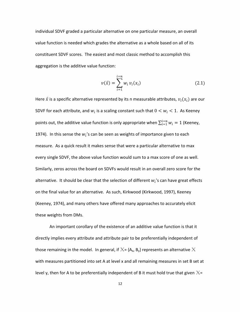
individual SDVF graded a particular alternative on one particular measure, an overall
value function is needed which grades the alternative as a whole based on all of its
constituent SDVF scores. The easiest and most classic method to accomplish this
aggregation is the additive value function:
Here is a specific alternative represented by its n measurable attributes, are our
SDVF for each attribute, and is a scaling constant such that . As Keeney
points out, the additive value function is only appropriate when (Keeney,
1974). In this sense the ’s can be seen as weights of importance given to each
measure. As a quick result it makes sense that were a particular alternative to max
every single SDVF, the above value function would sum to a max score of one as well.
Similarly, zeros across the board on SDVFs would result in an overall zero score for the
alternative. It should be clear that the selection of different ’s can have great effects
on the final value for an alternative. As such, Kirkwood (Kirkwood, 1997), Keeney
(Keeney, 1974), and many others have offered many approaches to accurately elicit
these weights from DMs.
An important corollary of the existence of an additive value function is that it
directly implies every attribute and attribute pair to be preferentially independent of
those remaining in the model. In general, if X= {Ax, By} represents an alternative X
with measures partitioned into set A at level x and all remaining measures in set B set at
level y, then for A to be preferentially independent of B it must hold true that given X=

13
{Ax, By} is preferred over Y= {Ax’, By}, then X should be preferred to Y for any choice of
level y on set B. Consider our notional example of where to go to lunch. Suppose that
restaurant X= {10 mi, $10, Delicious} and Y= {5 mi, $10, Moderate}. If our value
function is constructed to give higher weight to tastiness, we may very well have that X
is preferred over Y. Now consider that both restaurants decide to cut prices and the
alternatives now become X= {10 mi, $5, Delicious} and Y= {5 mi, $5, Moderate}. If Y is
now preferred over X ($5 nearby is too good a deal to pass up even if the food isn’t the
best), then my model is not preferentially independent.
As an important side note, there exists a similar but stronger independence
concept called utility independence. Keeney explains that for a single attribute x1 to be
utility independent of the remaining attributes preference order for lotteries involving
only changes in the levels of attributes in x1 does not depend on the levels at which the
remaining attributes are held fixed (Keeney, 1976). However, since utility independence
can be seen as the risk dependent analog to preferential independence, in value models
which do not consider risk (as is the case with our JIEDDO model), it is admissible to
treat any utility independence requirements as preferential independence
requirements.
Thorough pair wise proof of preferential independence in the fashion described
above can be very hard and tedious to identify and so it is no wonder that Carlsson et al.
argues that it is part of the habitual thinking of much of DA to simply assume that all
criteria are independent in order to maintain feasible solutions (Carlsson & Fuller, 1995).
14
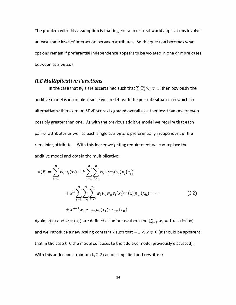
The problem with this assumption is that in general most real world applications involve
at least some level of interaction between attributes. So the question becomes what
options remain if preferential independence appears to be violated in one or more cases
between attributes?
II.E Multiplicative Functions
In the case that ’s are ascertained such that , then obviously the
additive model is incomplete since we are left with the possible situation in which an
alternative with maximum SDVF scores is graded overall as either less than one or even
possibly greater than one. As with the previous additive model we require that each
pair of attributes as well as each single attribute is preferentially independent of the
remaining attributes. With this looser weighting requirement we can replace the
additive model and obtain the multiplicative:
Again, v and are defined as before (without the restriction)
and we introduce a new scaling constant k such that (it should be apparent
that in the case k=0 the model collapses to the additive model previously discussed).
With this added constraint on k, 2.2 can be simplified and rewritten:

15
One of the advantages of this model is that it only requires one additional piece of
information (namely k) to be solicited from the DM. Looking at the following expansion
of the multiplicative form concerning only two attributes it becomes clear that the goal
is to account for both the individual contributions of the different attributes as well as
some combined multiplicative effect.
Keeney suggests a framework for eliciting the new scaling constant (Keeney, 1974)
which in essence is adjusting the weights for measures depending on their scores. A
look at Figure 3 shows
Figure 3: Power Additive Model
an example of how our overall utility score may increase as does our value from our
SDVF. The strategy is similar to that of constructing exponential SDVF and thus it is no
surprise that Kirkwood actually proves that the multiplicative model is equivalent to the
power additive model which has the exponential distribution at its heart (Kirkwood,
1997). It is worth pointing out that this equality also underlines that a multiplicative
model assumes the existence of an additive model; the multiplicative model simply
0
0.2
0.4
0.6
0.8
1
0 0.5 1
Utility
Utility

16
allows for a relaxation of the constraint on and stops short of defining value
interactions as unique values.
II.F Multilinear Functions
In the case that preferential independence cannot be established for all attribute
pairs and instead we are left only with preferential independence of single attributes we
can still establish a multilinear value function (Keeney, 1992):
This form is similar to the multiplicative function, but includes a separate scaling
constant for each pair of attributes, each triple of attributes and so on up to a constant
for the n-tuple of all attributes. The advantage of this approach is that it allows for
interactions of every level to be examined and quantified, however the main
disadvantage is that it can require a total of 2n-1 scaling constants to be solicited from
the decision maker. While detailed processes for soliciting the constants exist (Keeney,
1980), the length of the process may lead all but the most meticulous DM’s to submit
contradictory or unrepresentative opinions over time.

17
II.G Constructed Scales
Direct measures are almost always preferable over a constructed scale in DA. If
house prices are to be measured dollars is much more objective and universally
understood then a constructed scale of “Cheap, affordable, expensive”. Not only does
the constructed scale usually give diminished granularity, but it becomes harder to
define (cheap means different things to different people). Still, in situations where
there is no direct scale available a constructed scale remains a valid option. In this
fashion it is possible to combine two separate measures into one single constructed
measure either through way of functional transformation or by defining a combined
categorical. For example, in their value model for Army base closures Ewing et al
creates a weighted sum of square footage based on a quality standard in order to
measure the “General Instructional Facilities”. While this strategy proved helpful in this
particular case, Ewing sites obstacles in general application (Ewing, Tarantino, & Parnell,
2006):
In practice, we found it difficult to find an analogous mathematical
transformation for some of our measures. This left us with measures that were not
independent in terms of preference and therefore were inconsistent with the application
of an additive model.
In the absence of a convenient transformation, a categorical measure can be
constructed more simply by enumerating all relevant level combinations of the
interacting factors and assigning each one its own category. These categories can then
be valued and arranged to form a typical SDVF. Ewing makes strides in accurately

18
soliciting such data by arranging the categories within a matrix to better allow a DM to
visualize the changing levels of interactions, but this is at the cost of even more
solicitations and value comparisons. Sometimes however the violation of independence
may be foggier and require a different approach.
II.H Hidden Objectives Keeney describes hidden objectives as hidden agendas; “Those that are obscured
by the complexity of the decision situation are discovered, and those that are
intentionally obscured by a party to the decision are uncovered” (Keeney, 1992). In this
case all or some of the DM’s true values have not been well identified or defined and
results in either mutual exclusivity or preferential independence being violated. This
can mean either an examination of terms and definitions or more specifically some
dependency requiring the addition of one or more values to the model. A prime
example can be seen in the recommendations section of the 2008 JIEDDO VFT thesis by
Dawley et al (Dawley, Lenore, & Long, 2008):
After scoring the 30 sample proposals against the decision model in conjunction
with reviewing the comments of previous BIDS evaluators, the research team
determined that the value of Technical Risk is really the combination of two related
values—technical feasibility and technology readiness. Technical feasibility can best be
described as the answer to the question “What is the likelihood that this thing will
work?” Technology readiness usually assessed by the widely used Technology Readiness

19
Level (TRL) scale in Appendix A, answers the question “To what fidelity has this system
been proven?”
In short, analysts concluded that DM preferences were being violated by the
model’s scoring because the model was inaccurately attempting to measure a single
value which should actually have been decomposed further. Alternatively, the problem
may lie with the fact that there is an additional tradeoff between attributes which the
DM either does not realize or is unwilling to recognize. This can lead to the afore
mentioned multiplicative model in which perhaps two particular attributes may act as
partial substitutes for each other which can lead to a negative scaling constant k to
represent the value tradeoff (Keeney, 1992). Although difficult to see at times, hidden
objectives can usually be reintegrated into the original value model once uncovered.
II.I General Regression
In situations in which a DM is uncomfortable or unable to directly answer
questions about the value of particular attributes it may be more constructive to
evaluate a set of alternatives instead. As mentioned earlier, for a finite set of
alternatives AHP as well as several similar procedures exist which allow the DM to
systematically answer comparison questions until all but a certain number of
alternatives have been outranked. This concept can be extended to define weighting
coefficients for value models that can evaluate an indefinite set in by soliciting a
preordering of a smaller sample set of alternatives. One of the main restrictions of this
method is that it requires that the overarching value function must be assumed a priori

20
in order to avoid overburdening the DM. Although Stewart offers a methodology for
assuming an approximation of Keeney and Raffia’s multiplicative function discussed
earlier, it still requires the specific SDVFs to be defined separately (Stewart, 1981).
Figueira et al actually provide a new method which actually builds a set of additive value
functions by looking at not only preferences within a sample set of alternatives, but by
rating the intensity of preference (Figueira, Greco, & Slowinski, 2009). At their heart,
these methods and those like them allow a model to be constructed by looking at
alternatives more holistically in order to uncover the importance of the underlying
factors. Stewart agrees that the concept should even extend to allow for nonlinear
functions (Stewart, 1984), but to date there has been no extensive practice of these
methods and Kleindorfer et al even suggests that such methods should usually be
attempted lastly should ‘all else fail’ (Kleindorfer, Kunreuther, & Schoemaker, 1993).

21
III. Methodology
III.A Requirements
After reviewing existing strategies for dealing with interdependency within a
value model, it was decided that to be a desirable technique, a new method would first
need to be transparent. This is to say that not only the process but the finished product
would be both understandable and defendable by the DM without the assistance of the
analyst. As seen in Chapter 2, there already exists many procedures for creating
mathematically robust yet complex models for interdependency, but these models are
useless if the DM does not feel a sense of ownership of the process. The new model
should be one which the DM can explain, not a magic black-box function which they
must trust spits out their values on the other side.
Second, the new method must be repeatable. While the goal is to examine the
effect of measuring interactions within the JIEDDO model, the methodology should be
general enough to apply to any value model in which possible interactions have been
detected. Even the JIEDDO model itself is only as static as the DM and their opinions
and may require partial or complete reevaluation as the DM or JIEDDO’s priorities
rearrange; “…different individuals may look at the problem from different perspectives,
or they may disagree on the uncertainty or value of the various outcomes.” (Clemen &
Reilly, 2001).
Lastly, the new function should fit within the current structure of an additive VFT
hierarchy. The reasoning for this is twofold: First, with an existing VFT model like
22
JIEDDO, it is desirable to confront the issue of dependency without scrapping the
considerable amount of time and effort that went into its creation. This will allow for a
model to be corrected, over time if necessary, with less risk of DM solicitation burnout.
Second, like it or not the additive VFT model has rapidly become increasingly popular as
the choice for both business and military DM’s when faced with difficult decisions.
Whether it is Gen Fogleman facing the future military challenges of the Air Force
(Parnell, Conley, Jackson, Lehmkuhl, & Andrew, 1998) or oil companies trying to
capitalize on the increasing flood of available data and statistics (Coopersmith, Dean,
McVean, & Storaune, 2001), VFT has a considerable foothold of acceptance and by
working within its framework rather than outside, the chances of high ranking buy-in
increase considerably.
III.B Assumptions In an attempt to maintain the requirement of transparency, the new method will
be limited to at most two-way interactions of factors. Intuitively it becomes increasingly
burdensome for a DM to consider the impact of three or more factors all changing levels
at once. Statistically most models are dominated by single factors and low-level
interactions; according to the sparsity of effects principle most higher-order interactions
become negligible anyway (Montgomery, 2005).
In examining these two-way interactions, we will also make the assumption that
interaction between two factors effectively precludes both from being considered in any
other interaction. This restriction stems not from an inability to model such interactions

23
but from the fact that such a situation would point to a more fundamental problem with
the original VFT model. Take for example the situation in which it has been identified
that Factor A interacts with Factor B. Further, now consider that Factor A also interacts
with Factor C. The more factors that Factor A is linked to, the more likely it becomes
that perhaps the model would be better represented multiplicatively rather than
additively. As mentioned earlier there exist several methods for creating such a model
which could provide a better representation of the apparently sweeping importance of
Factor A as either a substitute for other factors or a scaling factor by which all others
must be subject to.
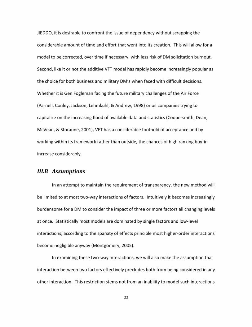
The model will also only consider interactions between those factors which share
both the same tier and objective within a hierarchy. Looking at Figure 4 we can see the
inherent issues involved with allowing interaction between any factors:
Figure 4: Allowed Interactions
The second interaction would effectively link two objectives on the above tier
and thus violate the rules of an additive VFT model. This does not mean that such an
interaction cannot exist nor does it mean that it is incapable of being modeled; the point
is simply that in such a case the two factors in question must ultimately share both tier
and parent objective. Once reorganized all that is left is to recalculate top tier weights
to coincide with the new lower tier global weight sums.

24
It should further be assumed that preferential independence as defined earlier
will already have been established between all factors except those which are the focus
of investigation. In these cases we can then make the assumption that while the two
specific factors interact, when considered jointly the pair remains independent from all
remaining factors.
Lastly, regardless of whether or not individual SDVFs have yet been established
for each factor, a suitable scale for each measure must exist for any modeling scheme
and thus we will assume that respective maximum and minimum values have been set.
Further, we will assume that two-way monotonicity is a desirable quality of the new
value function. This means that if Factor A and Factor B are to be combined and both
have measures which have been defined on a more-is-better scale, then it should follow
that as both increase the value of the new function should also increase or remain
constant. While there do exist unique situations in which overall value may actually
decrease as one or both factors increase (e.g. eating more ice cream is preferable up to
one bowl and eating more cookies is preferable up to four cookies, but when combined I
will get sick after eating half a bowl of ice cream and four cookies), but these situations
are not the norm and can usually be dealt with by reevaluating scales or objectives.
III.C Solicitation
A standard additive VFT model is made up of a group of SDVFs that in turn are
weighted and added together to score feasible alternatives. The goal of this process is
to create a new value function that would replace two SDVFs and bear their combined

25
weight. This new function will consider both constituent values and their interactions,
but will output a single value which can be aggregated normally back into the model.
The first step of this process is to identify which factors to investigate for
interactions. An advantage of the process is that once an initial hierarchy has been
created, an interactive function can be created before or after individual SDVFs have
been defined. This allows for hierarchies such as JIEDDO’s to be adjusted, but also saves
the time of soliciting SDVFs at all if a DM is convinced that the factors must be
considered together from the start. While any number of interactions can be tested, it
depends on the motivation and patience of the DM. It should also be explained to the
DM that after creation the new function can easily be tested for independence to
determine their advantage in place of SDVFs. Thus, time permitting, there is no harm in
investigating pairs in which suspicion of interaction is weaker should the DM desire.
Looking at the JIEDDO model once again, there are several specific areas of
possible interaction; consider for example Gap Impact and Time to counter.

26
Figure 5: Identified Interactions
After the factors have been chosen, the next step is to choose appropriate
breakpoints for continuous as well as large categorical measures. These points
ultimately will define the accuracy and granularity of the new function. Every additional
breakpoint will constitute extra solicitation on the part of the DM and it is therefore
recommended that the total number remain manageable. Likewise, it is best to choose
points along the scale which the DM feel represent tangible change (i.e. given a ten year
warranty is the best, it’s difficult to gauge how much six months is worth, but a year is
definitely 20% value). Due to the finite nature of categorical measures it is
recommended that as long the total number of categories remains reasonable that all
categories be evaluated as breakpoints to increase accuracy. In the continuous case
should the DM have no strong feeling about any particular points, the de facto strategy
Potential to
Defeat IED
1.00
Needed
Capability
.400
Operational
Performance
.350
Usability
.250
Gap Impact
.176
Classification
.056
Time to
Counter
.112
Technical
Performance
.110
Suitability
.056
Interoperability
.091
Technical Risk
.037
Fielding
Timeline
.056
Operations
Burden
.087
Work Load
.100
Required
Training
.063
Training
Time
.050
Program
Maturity
.013
# Tenets
Impacted
Primary Gap
Addressed
Classification
Level
Months Useful
Operation
Performance
Rating
Suitability
Rating
Interoperability
Issues
Technology
Readiness
Level
Months to
Fielding
% Maximum
Capacity
Interaction
Minutes per
Hour
Training Hours
Required
Training Level
Tenets
Impacted
.056

27
will be to simply divide the scale into equal increments. Applying this to the two chosen
factors achieves the breaks in Figure 6.
Figure 6: Breakpoints
It should be noted that Time to Counter is a continuous scale and as such could have
been broken at any point. Further, while the endpoints of the continuous scale could
easily be used if desired by the DM, they are avoided here in an attempt to force the
DM to think about specific values rather than being influenced by the fact that they are
at the extreme of one scale and overvalue their estimate. This follows well known DA
research which showed that not only was it difficult to extract accurate values very near
endpoints but that 5%, 50% and 95% values worked surprisingly well in defining a wide
range of distributions (Keefer & Bodily, 1983). Depending on the DM it may be
advisable to extend this strategy to categorical scales as well if the analyst feels there is
undue bias (i.e. solicited values are too tightly clustered). As stated earlier the
granularity to which the scales are divided is completely up to the DM and only depends
on the amount of time they are willing to commit to the process.
Once the breakpoints have been established, the next step is to solicit values
from the DM for each factor. This is done in a similar fashion to soliciting traditional

28
SDVFs, except for the main distinction that the DM will be valuing the different
breakpoints of one factor given the highest (or possibly second highest categorical if
bias is identified as mentioned above) breakpoint of the other factor. In the example,
since Gap Impact is a decreasing scale the task for the DM would be to assign decreasing
values between one and zero to G1 through G8 under the assumption that they are
guaranteed a Time to Counter of 54 months. The task is then repeated for Time to
Counter; given they are guaranteed a Gap Impact of G2 what value does the DM assign
to Time to Counter levels of 6, 18, 30, 42 and 54 months (again between zero and one,
but this time in increasing value). The results are shown in Tables 1 and 2. Once the
Table 1: Categorical Values Table 2: Continuous Break Values
tables have been solicited, a consistency and validation check must be completed.
First, based on their construction both tables will overlap at a single value.
Looking at Tables 1 and 2 this happens at G1 and 54 months. In order to consistently
represent the interactive value of the two factors this value must be the same in each
Level Value
G1 0.95
G2 0.90
G3 0.70
G4 0.35
G5 0.30
G6 0.20
G7 0.15
G8 0.10
None 0.05
Gap Impact Value
Given 54 Month
Time to Counter
Level Value
6 0.10
18 0.25
30 0.35
42 0.60
54 0.85
Time to Counter
Value Given Gap
Impact of G1

29
solicitation. If as in the example it does not, the DM must decide whether one or both
of their solicitations must be adjusted so that these interactions are ultimately
equivalent. Let us assume that our categorical values are deemed accurate but the
continuous scale must be adjusted resulting in the new values shown in Table 3.
Next, look at the jumps in value along the solicited scale. The new multi-
objective function will depend on linear interpolations between the solicited values in
Table 3. As such, larger jumps in value represent a larger chance of inaccurately
capturing intermediate values. Exponential functions have been shown to be robust in
Table 3: Adjusted Values
modeling DM values (Kirkwood & Sarin, 1980). Furthermore, in examining realistic
situations we see that the defining rho-value for such functions is rarely less than one
tenth of the overall range of possible factor levels (Kirkwood C. W., 1997).
Level Value
6 0.10
18 0.25
30 0.50
42 0.80
54 0.95
Time to Counter
Value Given Gap
Impact of G1

30
Figure 7: Piecewise linear v. exponential w/ rho=0.1
Based on these results and Figure 7 it is clear that in comparing any linear
section of a piecewise interpretation to an exponential representation of that same
section that the highest possible error is 66% of the original range. Thus, looking at the
values solicited in Table 3, for any adjacent values which differ by more than 0.15, we
will interpolate exponentially rather than linearly. This will ensure that any possible
discrepancies between interpolated values and those of the DM should be held to less
than 0.1. It should be noted that if this error margin is unacceptable to the DM, lower
tolerances are easily substituted at the cost of further solicitations as each exponential
interpolation requires one additional data point from the DM. Looking at Table 3, our
example requires two extra solicitations to account from the jump between 18 and 30
months as well as from 30 to 42. Kirkwood explains that the midvalue (i.e. what factor
level achieves mean value between the two endpoints) provides a convenient method
for calculating the function(Kirkwood C. W., 1997). Looking at Table 3 this amounts to
asking the question “If guaranteed a Gap Impact of G1, how much Time to Counter
would you require before reaching a value of 0.375?” Similarly, the jump from 30 to 42

31
months would be addressed by assessing the level to reach a value of 0.65. Tables 4 and
5 now show our complete data set.
Table 4: Categorical Values Table 5: Updated Continuous w/ Midvalues
III.D Processing
After completing solicitation with the DM, the data can now be processed into
the combined value function. As alluded to earlier, this is done by interpolating the data
in Tables 4 and 5 to fully define values to all possible ordered pairs of levels of our two
chosen factors. To this end, our two tables of solicited data can more appropriately be
seen in Table 6 as two dimensions of a common function.
Table 6: Two-Dimensional Value Matrix
Level Value
G1 0.95
G2 0.90
G3 0.70
G4 0.35
G5 0.30
G6 0.20
G7 0.15
G8 0.10
None 0.05
Gap Impact Value
Given 54 Month Time
to Counter
Level Value
6 0.10
18 0.25
20* 0.38
30 0.50
40* 0.65
42 0.80
54 0.95
* Exponential
Midvalues
Time to Counter
Value Given Gap
Impact of G1

32
It is important to note the addition of values to the far corners of Table 6. In the
same way that an ordinary SDVF must range from zero to one in value, so must our new
two-dimensional function. Thus it is logical that (60, G1) should represent a value of
one and (0, None) should represent a value of zero since they respectively represent the
combined best and worst of each measure.
Not only is this matrix largely sparse, but it does not account for an infinite
number of continuous points. Thus, a three step process is applied which will both fill
our matrix and provide functions for all intervening unaccounted continuous values.
Step 1. Looking at Table 6, it is useful to think of each row and each column in
terms of a SDVF, the main difference being that unlike a traditional value function, we
allow a different SDVF for every level each individual factor (e.g. a complete SDVF given
a Gap Impact of G2). SDVFs for remaining levels of each factor can now be determined
by examining and extending the relationship between adjacent cells. Consider the point
(42, G2); based on comparing values in the adjacent column we see that the DM’s value
for a Gap Impact of G2 given 54 months usefulness is approximately or 97.4% the
value of G1 given the same number of months. Using this information we could infer
that the DM would similarly assign (42, G2) a value equal to 97.4% of (42, G1). Since
(42, G1) has previously been solicited at 0.80 we are able to assign (42, G2) a value of
0.76. Two direct advantages follow from this process:

33
First, value calculations are consistent regardless of whether they are calculated
horizontally or vertically. Consider Table 7 where values have been solicited for a, x,
and y:
Table 7: Value Matrix
Looking at the equations below it is clear that b remains unchanged if calculated based
on the relationship between a and b instead of between x and y:
Second, extracting values in this manner explicitly maintains the two-way
monotonicity which was defined earlier. Original solicitation already requires that
and that , thus by solving for a and y in the preceding equations we can
show that
By extending the process to the interior of Table 6 these relationships continue
to hold and yield the new collection of values in Table 8. Note that although (0, None)
… a x
… b y
… … …Fact
or
A
Factor B
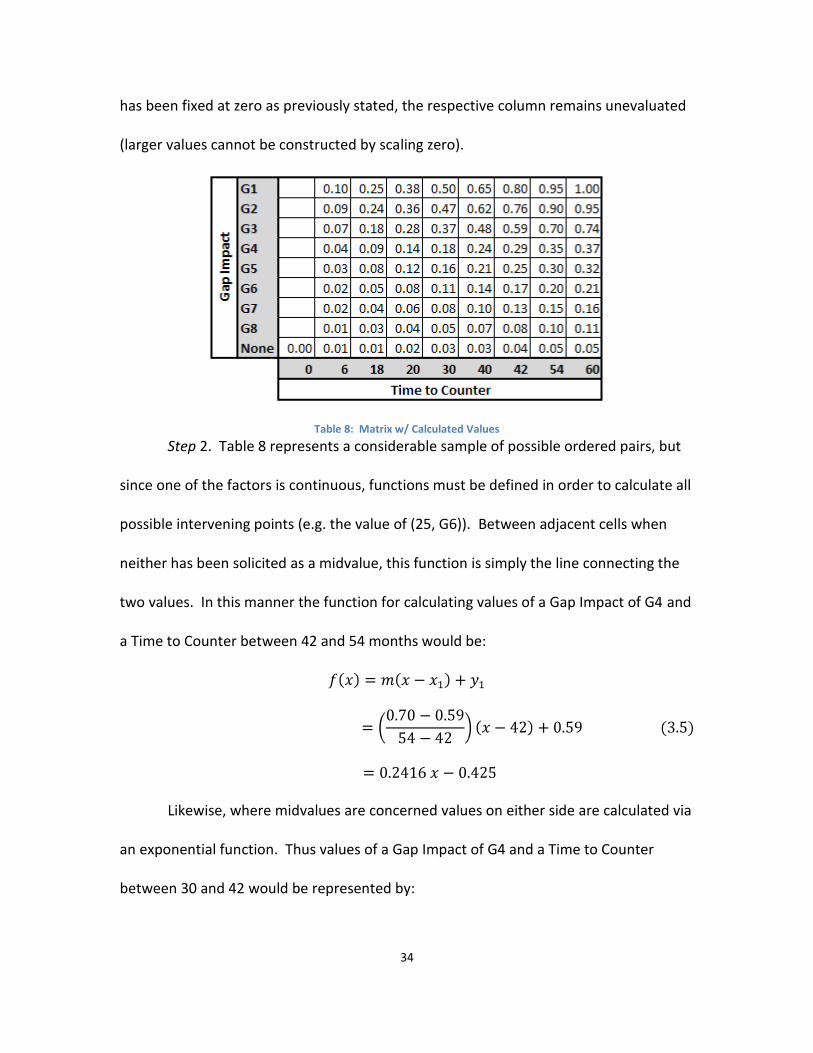
34
has been fixed at zero as previously stated, the respective column remains unevaluated
(larger values cannot be constructed by scaling zero).
Table 8: Matrix w/ Calculated Values
Step 2. Table 8 represents a considerable sample of possible ordered pairs, but
since one of the factors is continuous, functions must be defined in order to calculate all
possible intervening points (e.g. the value of (25, G6)). Between adjacent cells when
neither has been solicited as a midvalue, this function is simply the line connecting the
two values. In this manner the function for calculating values of a Gap Impact of G4 and
a Time to Counter between 42 and 54 months would be:
Likewise, where midvalues are concerned values on either side are calculated via
an exponential function. Thus values of a Gap Impact of G4 and a Time to Counter
between 30 and 42 would be represented by:

35
While the equation form differs slightly based on the solicited midvalue, the
general concept remains the same with the specific rho constant available in lookup
tables in many texts (Kirkwood C. W., 1997, p. 69). It is worth noting that while it is not
the case in this example, it is possible to have a situation in which both factors are
continuous. In these cases, values without adjacent values can be interpolated by first
interpolating the missing adjacent values and then interpolating based upon these new
numbers. It can be shown that given a situation such as Table 9 where the highlighted
cells have been interpolated, the center cell evaluates the same regardless of whether it
is interpolated horizontally between values of 3.6 or vertically.
Table 9: Two-Way Interpolation
Step 3. In situations where endpoints have not been solicited, values cannot be
calculated as in step 1. Unlike b in Table 7, end columns and rows may not have the
required solicited adjacent values in order to be calculated. Without two adjacent
values to interpolate between, these values are extrapolated by simply extending the
adjacent function (either linear or exponential) established in step 2. However, since

36
the new two-dimensional function must only range between zero and one, when
extrapolating a maximizing row or column, we take the minimum between the
extrapolation and one. Similarly when extrapolating a minimizing row or column, we
must take the maximum between the extrapolation and zero. The only remaining
possible situation exists when an adjoining end row and end column both must be
extrapolated which implies two possible values for the corner of their intersection. In
these cases the difference is usually negligible and it is left to the DM to choose
between the larger or smaller estimate. In the absence of DM input it is suggested to
err on the side of caution and opt for the larger of the two values as it is generally
preferable by a DM to slightly overvalue an alternative rather than to slightly undervalue
it.
Combining these three steps together the process not only fully populates the
initially sparse Table 6 into the now robust Table 10 but also provides definition of all
functions required for any possible ordered pair of levels from the original two factors.
It should be clear that once presented with the final functions, if the DM expresses
concern for any inaccuracy, any of the original levels may be re-solicited in addition to
intermediate levels for increased granularity. Once defined, the three step process
described above is automatic and instant and can be rerun as many times as necessary
without any extra burden on the DM.

37
Table 10: Two-Dimensional Value Matrix
By considering each ordered pair as input to this family of functions, the original
two weighted contributions to the model’s overall value function can now be replaced
with the single output of our new function scaled by the sum of the weights of the two
factors.
The original JIEDDO value function is simply edited by replacing the two
highlighted contributions with +.288 v(TimeToCounterGap), where v(TimeTo
CounterGap) represents the new combined value function. The weights of the new
value function still sum to one, and based on the assumptions now (given all suspected
interactions within the model have been explored) meet the preferential independence
requirement between factors necessary to accurately score alternatives.

38
IV. Results & Analysis
IV.A Overview
This chapter starts with the original JIEDDO value model and builds two
additional models; an illustrative example created by the researcher and results solicited
from a recently deployed Marine Engineering Commander. Both models are created by
expanding on the original model to allow for interactions using the proscribed
methodology from chapter three. Additionally, two-dimensional value functions are
created by directly soliciting all possible interaction values (e.g. all 81 values found in
Table 10). By using thirty JIEDDO proposals (each of whose factors were scored by the
original JIEDDO model team of Dawley et al) deterministic analysis is performed on all
three models to determine the credibility of the value function interpolation
methodology. Main results are addressed within the illustrative example while the
second model closes the chapter by identifying several areas of possible concern in
practical implementation.
IV.B Measure Creation
Throughout the proceeding four sections, the researcher takes on the role of the
DM in analyzing the JIEDDO model. This provides a surrogate for the purpose of
demonstrating the methodology. Further, as this model is intended to be applicable to
other scenarios including future JIEDDO DM changes, validation of the model depends
not on the depth of C-IED knowledge on the part of the DM but rather on the
consistency between the alternative rank structures resulting from both methods.
39
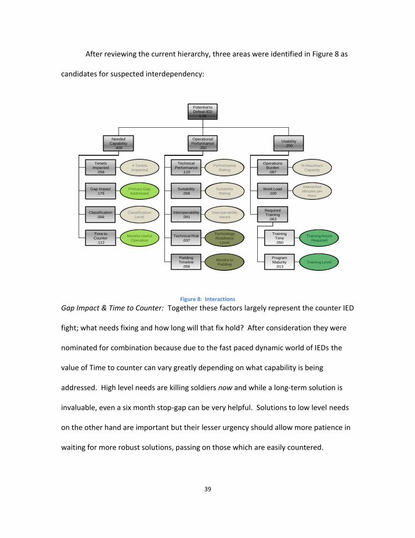
After reviewing the current hierarchy, three areas were identified in Figure 8 as
candidates for suspected interdependency:
Figure 8: Interactions
Gap Impact & Time to Counter: Together these factors largely represent the counter IED
fight; what needs fixing and how long will that fix hold? After consideration they were
nominated for combination because due to the fast paced dynamic world of IEDs the
value of Time to counter can vary greatly depending on what capability is being
addressed. High level needs are killing soldiers now and while a long-term solution is
invaluable, even a six month stop-gap can be very helpful. Solutions to low level needs
on the other hand are important but their lesser urgency should allow more patience in
waiting for more robust solutions, passing on those which are easily countered.
Potential to
Defeat IED
1.00
Needed
Capability
.400
Operational
Performance
.350
Usability
.250
Gap Impact
.176
Classification
.056
Time to
Counter
.112
Technical
Performance
.110
Suitability
.056
Interoperability
.091
Technical Risk
.037
Fielding
Timeline
.056
Operations
Burden
.087
Work Load
.100
Required
Training
.063
Training
Time
.050
Program
Maturity
.013
# Tenets
Impacted
Primary Gap
Addressed
Classification
Level
Months Useful
Operation
Performance
Rating
Suitability
Rating
Interoperability
Issues
Technology
Readiness
Level
Months to
Fielding
% Maximum
Capacity
Interaction
Minutes per
Hour
Training Hours
Required
Training Level
Tenets
Impacted
.056

40
Technical Risk & Fielding Timeline: War fighters understand that new technology can
take time to make it to the field, but that patience is linked to the ultimate effectiveness
of the technology once it reaches the field. A solution with very low risk maintains its
value much more easily as its fielding time is pushed forward whereas high risk
proposals with long timelines quickly become difficult to defend.
Training Time & Program Maturity: A training time for a program which has not been
developed yet is an estimate at best. As the maturity of such programs is better
established the value of training time estimates should increase as well.
Tables 11 through 16 show the solicited breakpoints and associated values for
each interaction defined above. While inspection of the tables reveals seven instances
of value jumps above 0.15, once midvalues were solicited it became clear that in this
particular case there was no difference between using linear or exponential
interpolation (i.e. the two shared the same midpoint). Using the methods from Chapter
three these six tables were used to generate the full two dimensional range of values for
each of the three newly combined measures which are available in Appendix A.
Solicitation of each table took less than five minutes and, while the researcher is
conversant in such tasks, test solicitations with several other non-DA participants
proved that each table took at most ten minutes to explain and solicit keeping the entire
process under one hour.
Three additional direct solicitations were then accomplished for each interaction
to test the validity of the mathematically interpolated and extrapolated values. As
shown in Table 17, each of these solicitations was a complete enumeration of the two-

41
dimensional space as defined by the breakpoints. It should be immediately clear that
this requires not only many more inputs by the DM but also many more comparisons to
ensure that two-way monotonicity is maintained. Assuming n breakpoints for each
individual measure the original method requires only 2n inputs and a minimum of 2(n-1)
comparisons to ensure monotonicity. By contrast, the completely enumerated
solicitation requires n2 inputs from the DM and at least 2n2-2n comparisons to ensure
monotonicity. In our particular example of Gap Impact and Time to counter this means
that our required inputs jump from 18 to 99 and our comparisons from 16 to 180. Time
wise this amounted to nearly two hours of work when accomplished solely by the
researcher. In comparison the only outside subject willing to devote the time to
complete solicitation took four one hour sessions over four days and resulted in a table
which still contained several instances of decreasing values. This underlines one of the
main difficulties associated with constructed scales such as those put forth by Ewing et
al in Chapter 2. Even though a visual representation such as Table 17 aids in soliciting
the data more accurately, what Ewing and his team gain in visual simplicity they quickly
lose to the sheer number of comparisons demanded from the DM. In addition to the
2n2-2n monotonicity comparisons, Ewing et al require up to an additional or
comparisons to ensure consistency of the DM. Again, in this particular example
this amounts to requesting over 4,000 additional value judgments from the DM, a task
unlikely to be accomplished.
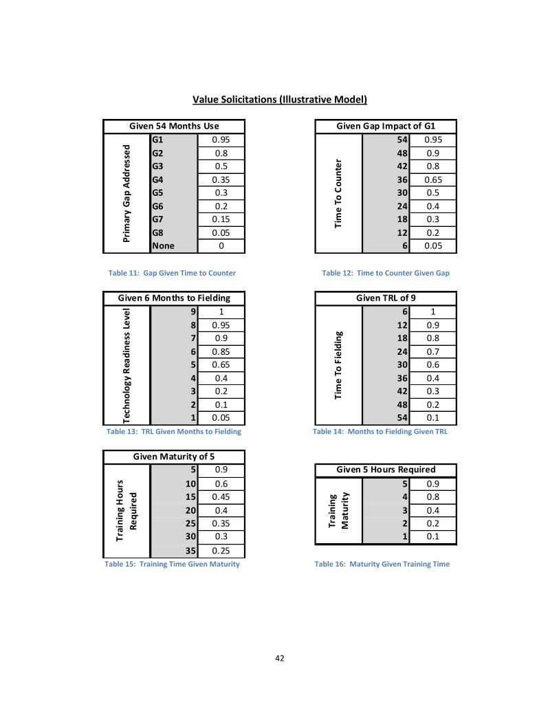
42
Value Solicitations (Illustrative Model)
Table 11: Gap Given Time to Counter Table 12: Time to Counter Given Gap
Table 13: TRL Given Months to Fielding Table 14: Months to Fielding Given TRL
Table 15: Training Time Given Maturity Table 16: Maturity Given Training Time
G1 0.95 54 0.95
G2 0.8 48 0.9
G3 0.5 42 0.8
G4 0.35 36 0.65
G5 0.3 30 0.5
G6 0.2 24 0.4
G7 0.15 18 0.3
G8 0.05 12 0.2
None 0 6 0.05
Given 54 Months UseP
rim
ary
Ga
p A
dd
ress
ed
Given Gap Impact of G1
Tim
e T
o C
ou
nte
r
9 1 6 1
8 0.95 12 0.9
7 0.9 18 0.8
6 0.85 24 0.7
5 0.65 30 0.6
4 0.4 36 0.4
3 0.2 42 0.3
2 0.1 48 0.2
1 0.05 54 0.1Tec
hn
olo
gy
Rea
din
ess
Le
vel
Tim
e T
o F
ield
ing
Given TRL of 9Given 6 Months to Fielding
5 0.9
10 0.6 5 0.9
15 0.45 4 0.8
20 0.4 3 0.4
25 0.35 2 0.2
30 0.3 1 0.1
35 0.25
Tra
inin
g
Mat
uri
ty
Tra
inin
g H
ou
rs
Re
qu
ire
d
Given Maturity of 5
Given 5 Hours Required
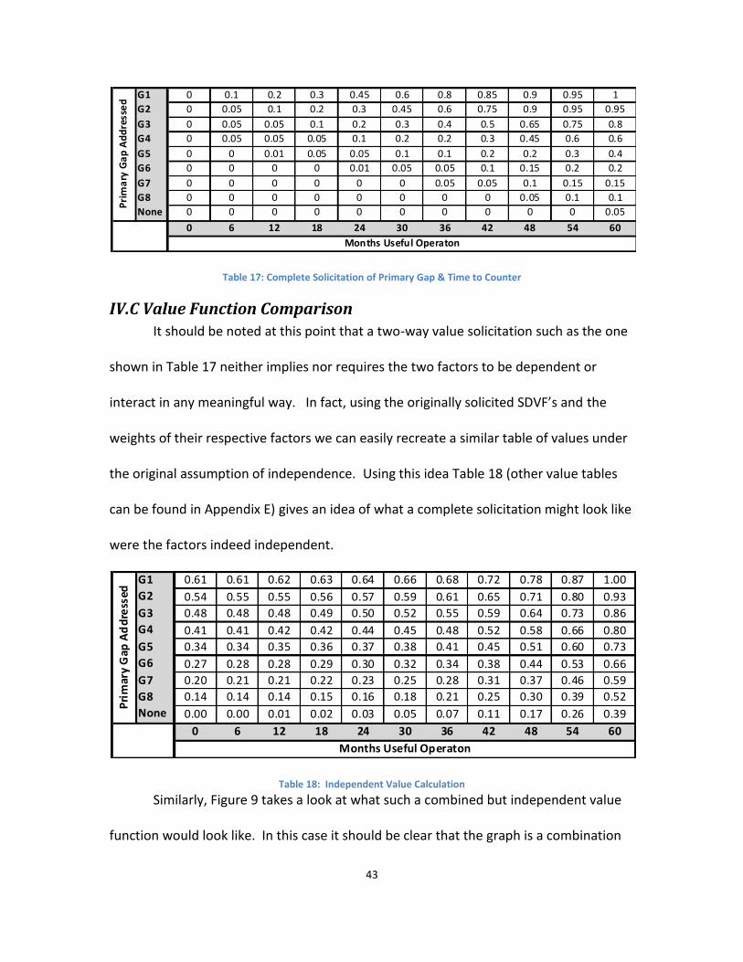
43
Table 17: Complete Solicitation of Primary Gap & Time to Counter
IV.C Value Function Comparison
It should be noted at this point that a two-way value solicitation such as the one
shown in Table 17 neither implies nor requires the two factors to be dependent or
interact in any meaningful way. In fact, using the originally solicited SDVF’s and the
weights of their respective factors we can easily recreate a similar table of values under
the original assumption of independence. Using this idea Table 18 (other value tables
can be found in Appendix E) gives an idea of what a complete solicitation might look like
were the factors indeed independent.
Table 18: Independent Value Calculation
Similarly, Figure 9 takes a look at what such a combined but independent value
function would look like. In this case it should be clear that the graph is a combination
G1 0 0.1 0.2 0.3 0.45 0.6 0.8 0.85 0.9 0.95 1
G2 0 0.05 0.1 0.2 0.3 0.45 0.6 0.75 0.9 0.95 0.95
G3 0 0.05 0.05 0.1 0.2 0.3 0.4 0.5 0.65 0.75 0.8
G4 0 0.05 0.05 0.05 0.1 0.2 0.2 0.3 0.45 0.6 0.6
G5 0 0 0.01 0.05 0.05 0.1 0.1 0.2 0.2 0.3 0.4
G6 0 0 0 0 0.01 0.05 0.05 0.1 0.15 0.2 0.2
G7 0 0 0 0 0 0 0.05 0.05 0.1 0.15 0.15
G8 0 0 0 0 0 0 0 0 0.05 0.1 0.1
None 0 0 0 0 0 0 0 0 0 0 0.05
0 6 12 18 24 30 36 42 48 54 60
Pri
ma
ry G
ap
Ad
dre
sse
d
Months Useful Operaton
G1 0.61 0.61 0.62 0.63 0.64 0.66 0.68 0.72 0.78 0.87 1.00
G2 0.54 0.55 0.55 0.56 0.57 0.59 0.61 0.65 0.71 0.80 0.93
G3 0.48 0.48 0.48 0.49 0.50 0.52 0.55 0.59 0.64 0.73 0.86
G4 0.41 0.41 0.42 0.42 0.44 0.45 0.48 0.52 0.58 0.66 0.80
G5 0.34 0.34 0.35 0.36 0.37 0.38 0.41 0.45 0.51 0.60 0.73
G6 0.27 0.28 0.28 0.29 0.30 0.32 0.34 0.38 0.44 0.53 0.66
G7 0.20 0.21 0.21 0.22 0.23 0.25 0.28 0.31 0.37 0.46 0.59
G8 0.14 0.14 0.14 0.15 0.16 0.18 0.21 0.25 0.30 0.39 0.52
None 0.00 0.00 0.01 0.02 0.03 0.05 0.07 0.11 0.17 0.26 0.39
0 6 12 18 24 30 36 42 48 54 60
Pri
mar
y G
ap A
dd
ress
ed
Months Useful Operaton
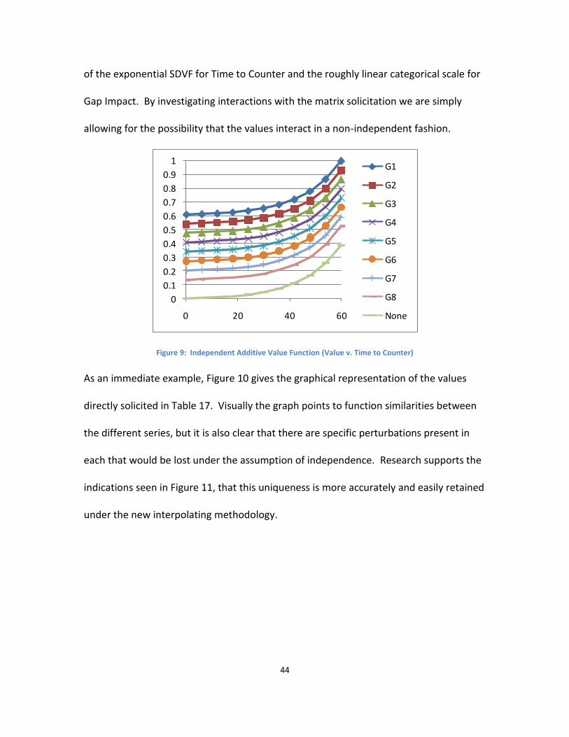
44
of the exponential SDVF for Time to Counter and the roughly linear categorical scale for
Gap Impact. By investigating interactions with the matrix solicitation we are simply
allowing for the possibility that the values interact in a non-independent fashion.
Figure 9: Independent Additive Value Function (Value v. Time to Counter)
As an immediate example, Figure 10 gives the graphical representation of the values
directly solicited in Table 17. Visually the graph points to function similarities between
the different series, but it is also clear that there are specific perturbations present in
each that would be lost under the assumption of independence. Research supports the
indications seen in Figure 11, that this uniqueness is more accurately and easily retained
under the new interpolating methodology.
0
0.1
0.2
0.3
0.4
0.5
0.6
0.7
0.8
0.9
1
0 20 40 60
G1
G2
G3
G4
G5
G6
G7
G8
None

45
Figure 10: Directly Solicited Combined Value Functions (Value v. Time to Counter)
Figure 11: Interpolated Combined Value Functions (Value v. Time to Counter)
IV.D Alternative Scoring & Ranking
Appendix B lists 30 counter IED proposals submitted to JIEDDO in 2007. Each of
the original 13 factors was scored by Dawley et al for each proposal (proposal titles have
been removed for classification reasons). The first column of Table 19 provides the
final score for each proposal based on the model in equation 4.1 which integrates all
three direct complete combined solicitations. Column two represents the same model
0
0.1
0.2
0.3
0.4
0.5
0.6
0.7
0.8
0.9
1
0 20 40 60
G1
G2
G3
G4
G5
G6
G7
G8
None
0
0.1
0.2
0.3
0.4
0.5
0.6
0.7
0.8
0.9
1
0 20 40 60
G1
G2
G3
G4
G5
G6
G7
G8
None

46
but replaces each combined value function with interpolation according to the
proscribed methodology.
V(X) = .056 v(Tenets) + .288 v(Gap&Counter) + .056 v(Class)
+ .11 v(TechPerf) + .056v(Suit) + .091 v(Interop)
+ .093 v(TechRisk&Fielding) + .087 v(OpsBurden) (4.1)
+ .1 v(Workload) + .063 v(TrngTime&Maturity)
While certain changes in score are immediately evident, the data in Table 19 is
purely ordinal meaning that the scores themselves have meaning only in the ranking
which they provide to the data set. These ranks are given in Table 20 and are ordered
based on the “Complete Solicitation” scores for later analysis. Two important
observations of Table 20 can be made simply by inspection even before any type of
statistical analysis. While not identical in rank, complete and partial solicitation with
interpolation both yield the same top ten alternatives and the same bottom ten. This is
specifically important to an organization such as JIEDDO where the model is intended as
a tool to filter alternatives rather than to choose a single winner. This would mean that
a DM would receive the same reduced set of alternatives to examine between these
newly solicited models. These conjectures can be better quantified with nonparametric
rank testing.

47
Table 19: JIEDDO Alternative Scores

48
Table 20: JIEDDO Alternative Rankings

49
IV.E Rank Testing
Due to the afore mentioned ordinal nature of our data, we are unable to make
any assumptions as to the distributions from which they are pulled and cannot use
typical parametric tests in examining the data. Fortunately, there exist many
nonparametric tests which are distribution free making up in robustness what they may
lose in simplicity. While many nonparametric tests seek to give specific information
about the distribution from which the data is pulled, we are interested instead in the
correlation between rankings. Kendall’s Tau and Spearman’s Rho are both widely
accepted as methods to this end. While other measures exist, these two statistics are
uniquely appropriate in measuring the correlation of ranking pairs and both rest on
relatively simple assumptions. The two tests are considered to be equivalent and only
differ in their interpretation of results (Bolboaca & Jantschi, 2006). Spearman’s Rho
yields a correlation coefficient while Kendall’s gives a slightly more simple interpretation
of the correlation as a probability. For these reasons we will use Kendall’s Tau in our
analysis.
where:
C = # of Y pairs in natural order
D = # of Y pairs in reverse order
n = # of total (X,Y) observations

50
Like most nonparametric statistics, Kendall’s Tau has very few critical
assumptions (Pett, 1997):
1. The randomly selected data are sets of paired observations (X, Y) that have
been collected from the same subjects.
2. The two continuous variables, X and Y, are measured on at least an ordinal
scale.
Using the alternative scores as our X and Y, it should be clear that these
assumptions are well met and Kendall’s Tau is calculated based on the information in
Table 20. Since the rankings achieved from complete solicitation simply permit rather
than require that factors interact, it represents our ideal ranking. The remaining ranking
represents a way in which to estimate this ideal, through interpolation of data. Thus by
defining the complete solicitation scores as our X variables the remaining ranking is used
as Y’s to measure the level of correlation with the ideal set.
To calculate Kendall’s Tau we must first count both the number of concordant
and discordant pairs. Looking again at Table 19, this entails identifying all possible score
pairs in our non-ordered column and counting how many of those pairs are in natural
order (i.e. increasing) and how many are in reverse order (i.e. decreasing). These
concordances, calculated in Appendix C, are then fed into equation 4.2:
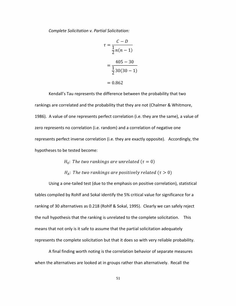
51
Complete Solicitation v. Partial Solicitation:
Kendall’s Tau represents the difference between the probability that two
rankings are correlated and the probability that they are not (Chalmer & Whitmore,
1986). A value of one represents perfect correlation (i.e. they are the same), a value of
zero represents no correlation (i.e. random) and a correlation of negative one
represents perfect inverse correlation (i.e. they are exactly opposite). Accordingly, the
hypotheses to be tested become:
Using a one-tailed test (due to the emphasis on positive correlation), statistical
tables compiled by Rohlf and Sokal identify the 5% critical value for significance for a
ranking of 30 alternatives as 0.218 (Rohlf & Sokal, 1995). Clearly we can safely reject
the null hypothesis that the ranking is unrelated to the complete solicitation. This
means that not only is it safe to assume that the partial solicitation adequately
represents the complete solicitation but that it does so with very reliable probability.
A final finding worth noting is the correlation behavior of separate measures
when the alternatives are looked at in groups rather than alternatively. Recall the

52
similarity within the top ten choices that was recognized earlier on. This is important to
JIEDDO and similar organizations in which rather than picking a single winner the model
is intended to provide a refined group for the DM to choose from. In these situations
the DM may take the top ten model-provided alternatives and choose five from that
group. In this manner a DM can look at successive groupings in order to compare
alternatives without looking at the entire set.
Table 21: Group Ranking Comparisons
Table 21 underlines another strength of the partial solicitation model by comparing the
average rankings of successively larger groupings found in Appendix D. The partial
solicitation continues to remain strongly correlated, maintaining significance to an alpha
of .005 up to a group size of five.
IV.F Sensitivity Analysis
After a value model has been created and weights assigned to all objectives,
sensitivity analysis allows the DM to see how sensitive the alternative ranking is to
changes in individual weights. As the purpose of this paper is to introduce an alternate
measure construction and not question the particular weights chosen it is useful to
compare the respective sensitivity analyses of the two methods. For the sake of
Complete v.
Partial
τ α=.05 α=.025 α=.005
1 (n-30) 0.862 0.218 0.255 0.333
3 (n=10) 0.887 0.467 0.511 0.644
5 (n=6) 1 0.733 0.867 1
Group
Size
Critical Values

53
simplicity we examine only the top tier weights. Figures 12 and 13 represent each
alternative as a different line.
Figure 12: Needed Capability Sensitivity Analysis (Original Model)
Figure 13: Needed Capability Sensitivity Analysis (Complete Solicitation)
While it seems that neither model is completely insensitive to weight change,
the breakpoints in weight at which alternatives switch rank appear to be more tightly
clustered and fewer in number in the combined model over the original. Further, by
combining factors the new model has reduced the overall number of measures and
likewise reduced the number of sensitivities which require analysis. Not only does this
0
0.1
0.2
0.3
0.4
0.5
0.6
0.7
0.8
0.9
1
0 0.2 0.4 0.6 0.8 1
Sco
re
Weight
0
0.1
0.2
0.3
0.4
0.5
0.6
0.7
0.8
0.9
1
0 0.2 0.4 0.6 0.8 1
Sco
re
Weight

54
make sense but it supports two of the chief tenets of a VFT hierarchy; small size and
operability (Kirkwood C. W., 1997).
The clustering result may owe more to chance than construction as the
remaining sensitivity charts in Appendix F fail to show as stark a difference, but it does
offer further proof that the combined model may have additional specific advantages as
a filtering tool. Eight out of ten of the top alternatives in the combined model are very
closely related in their sensitivity (average slope difference of 0.13) represented in
Figure 12. This means that as weights change the alternative rankings shuffle mostly
within specific groupings rather than spontaneously from first to last.
IV.F Marine Model and Additional Findings
After creating and analyzing the previous illustrative model, the methodology
was ultimately reapplied to an actual acting Marine Commander with extensive C-IED
experience recently returned from deployment to Iraq. The corresponding data and
rank analysis can be found along with the first solicitation in the attached appendices.
Three specific points stand out in comparison to the previous implementation of the
methodology.
First and most importantly, the methodology continues to exhibit a strong ability
to correctly model a DM’s explicit combined values. Recalculating Kendall’s Tau for our
new rank comparisons we see a statistic of 0.908 between the full and partial
solicitation of the commander. The model also remains strongly correlated as
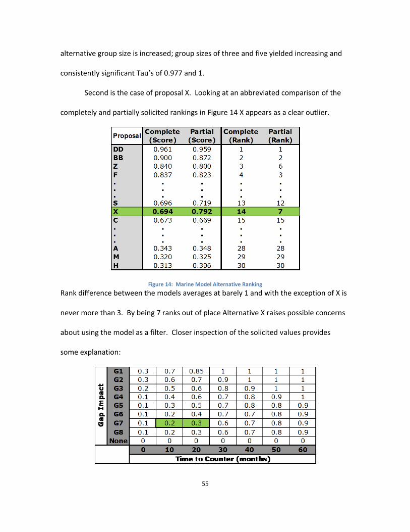
55
alternative group size is increased; group sizes of three and five yielded increasing and
consistently significant Tau’s of 0.977 and 1.
Second is the case of proposal X. Looking at an abbreviated comparison of the
completely and partially solicited rankings in Figure 14 X appears as a clear outlier.
Figure 14: Marine Model Alternative Ranking
Rank difference between the models averages at barely 1 and with the exception of X is
never more than 3. By being 7 ranks out of place Alternative X raises possible concerns
about using the model as a filter. Closer inspection of the solicited values provides
some explanation:

56
Figure 15: Directly Solicited Values
Figure 16: Partially Solicited Values w/ Interpolation
While the blue solicited row and column in Figure 16 perfectly matches their
counterparts in Table 15, the values are very tightly clustered near the high end and give
very little differentiation between levels to interpolate upon. As many of the
alternatives scored high on one or both of the measures this did not prove to be a
problem in general. Alternative X however possessed a Gap Impact of G7 and a Time to
Counter of only 12. As the interpolation breaks down near zero this leads to a
difference in value of 0.364 between the complete and partial model and an overall
score difference of 0.105. This disparity is singularly responsible for the misplacement
of X and significantly lowers the overall Kendall’s Tau. As discussed in future research
this would appear to be an issue of choosing at which level to solicit values on which to
interpolate those remaining and merits further investigation.

57
Lastly, while sensitivity analysis charts in Appendix F for the Needed Capability
still exhibit a certain level of the clustering phenomenon mentioned earlier, the
remaining charts seem to support the supposition that this is more likely a coincidence
of these particular measures and not a general result of the methodology.

58
V. Conclusions and Recommendations
This chapter provides a summary of the research presented, outlines key
contributions to JIEDDO and the field of decision analysis and submits several
suggestions for future research in the area.
V.A Research Review
VFT models have always depended on assumptions which require little work to
understand but much more to empirically prove. Not least amongst these is the
assumption of preferential independence. This research has investigated past methods
for creating robust decision models not bound by the assumption of preferential
independence and has developed a simple understandable process for creating such a
model.
As a case study JIEDDO provided a key example of a decision process modeled
through VFT but plagued by suspicions of independence violations. Building on the
original additive model, scored alternative set and accompanying research accomplished
by Dawley et al it was possible to create and validate the new methodology with
minimal interaction from JIEDDO representatives. By applying mathematical
interpolation a model which closely matched an exhaustive enumeration of DM values
was created which greatly reduced the number of required inputs from the DM and fit
within the established VFT hierarchy. This has the added advantage of developing a
method which is neither DM nor decision dependent. The new model was validated not
59
against how accurately it represented the specific JIEDDO decision process, but rather
how consistently and accurately it was able to capture the interactive values of a DM in
comparison to the more robust but lengthy enumeration process. This validation was
accomplished through the application of non-parametric rank tests.
V.B Contributions
Parallel research into the validity of the current JIEDDO value model has been
pursued by measuring its correlation to proposals approved by the organization without
the aid of the model. The research presents evidence which strongly suggests the
accuracy of the additive model in reflecting actual JIEDDO decisions (Willy, 2009). The
final results of this research not withstanding; this does not diminish the importance or
contribution of the presented research to JIEDDO. JIEDDO is unique among military
organizations in its ability and necessity to quickly adjust its mission to the ever
changing battle presented by IEDs. While the independent additive model currently
meets JIEDDO’s needs, it would be naïve to assume that this will always be the case.
The current model is only as accurate as the current doctrine and leadership, both of
which have changed over the years. Our methodology allows for reevaluation of the
model without complete re-accomplishment.
As a high-profile, high-budget joint organization JIEDDO is the target of intense
governmental oversight from many directions. As a result any decision model
implemented by JIEDDO will more than likely be the immediate target of scrutiny as to
its value to the program and taxpayers. By considering interactions our methodology

60
sidesteps the difficulty in explaining and proving preferential independence and instead
offers an immediate and simple answer for any with questions about synergistic effects
of certain factors; better to answer a question than attempt to explain its irrelevancy.
As stated earlier, a key characteristic of our methodology is its applicability
beyond JIEDDO. The methodology was purposefully created as a tool to work in
cooperation with established VFT methods. Since the methodology is based on
independent solicitation and not established SDVFs it is equally capable of both creating
combined functions from scratch during the initial model construction if the DM insists
on factors with known interdependence or creating combined functions after SDVFs
have been created if interdependency becomes suspected and must be tested.
V.C Future Research
Throughout the course of this research there have been several avenues for
improvement upon or extensions of the current methodology which were unable to be
pursued due to time and resource restrictions:
1. Reevaluation of the JIEDDO model: As mentioned earlier, the purpose of this
research was to develop a new methodology for capturing interactive values, not
to specifically “fix” the JIEDDO model. As the original model developed by
Dawley et al has yet to be implemented it would be interesting to work with the
actual JIEDDO DM and attempt to modify the current model through application

61
of our methodology and measure the effects of the new model both on
alternative ranking and DM and SME acceptance.
2. Higher dimension interaction consideration: This research has limited itself to
two-dimensional interactions of factors for previously discussed reasons. In
theory however the same solicitation concepts could be extended to any level of
interaction. The question would seem to be to find at what point do the number
and difficulty of solicitations outweigh the advantages of the more specifically
defined holistic model.
3. Independent determination of value functions: Prior research has been done on
comparing the VFT models and decisions made by a group working together
versus individually (Gezeravci, 2008). Many decisions (including JIEDDO to a
degree) are less the result of a single DM and more the culmination of a group of
SME’s. Determining the combined values required for the new methodology can
be increasingly difficult depending on the technical level of the measure. How
would the model and its accuracy be affected if after interaction pairs were
identified by the DM, specific SME’s were responsible for providing the required
value inputs?
4. Further validation of the methodology with a more robust sample set: The
current set of 30 alternatives used to test the methodology represents a
relatively small number in comparison to the total alternatives received by an
organization such as JIEDDO. Furthermore, the individual factor scoring for the
alternatives was accomplished by AFIT researchers rather than actual JIEDDO

62
SME’s. In order to provide more useful results to JIEDDO it is suggested to solve
these inadequacies as well as factoring in additional information about proposals
such as selection status and ultimate field effectiveness.
5. Comparison of methodology across several separate decisions: Research would
seem to support the extension of our methodology beyond JIEDDO but would be
considerably reinforced by the explicit application to several different hierarchies
and at different points within the process (e.g. before and after the creation of
SDVFs).
6. Effects of breakpoint selection on value solicitation: In Chapter 3 breakpoints
were chosen evenly and were solicited at either the highest or near highest level
of factors. There may be advantages to be gained by a varying the number and
distribution of breakpoints. Further, would the model be improved or degraded
if solicitations were based on midrange or lower values rather than higher.
V.D Summary
Violation of preferential independence within decision models is nothing new
nor is it something for which there does not exist a list of solutions. Unfortunately the
difficulty of most of these solutions either in understanding or implementation has
often led some DMs to ignore such violations in an attempt to embrace simpler models.
The methodology presented within this research greatly reduces the need for such a
tradeoff by offering both robustness and simplicity with mathematical techniques no
more complex than those already associated with simple VFT decision models.

63
Appendix A
A.1: Directly Solicited Value Matrices (Researcher)

64
A.2: Directly Solicited Value Matrices (Marine Commander)
G1 0.3 0.7 0.85 1 1 1 1
G2 0.3 0.6 0.7 0.9 1 1 1
G3 0.2 0.5 0.6 0.8 0.9 1 1
G4 0.1 0.4 0.6 0.7 0.8 0.9 1
G5 0.1 0.3 0.5 0.7 0.8 0.8 0.9
G6 0.1 0.2 0.4 0.7 0.7 0.8 0.9
G7 0.1 0.2 0.3 0.6 0.7 0.8 0.9
G8 0.1 0.2 0.3 0.6 0.7 0.8 0.9
None 0 0 0 0 0 0 0
0 10 20 30 40 50 60
Gap I
mpact
Time to Counter (months)
3 0.2 0.5 0.8 1 1 1 1
2 0.1 0.5 0.7 1 1 1 1
1 0.1 0.3 0.5 0.8 1 1 1
0 0 0 0 0 0 0 0
Above TS TSSEC/
NONFORNSEC/REL
CONFI-
DENTIALFOUO UNCLASS
Ten
ets
Add
ressed
Classification
5 0.3 0.3 0.3 0.4 0.7 0.9 1
4 0.2 0.2 0.2 0.3 0.7 0.8 1
3 0.1 0.1 0.1 0.2 0.6 0.8 1
2 0 0.1 0.1 0.2 0.6 0.8 1
1 0 0.1 0.1 0.2 0.5 0.8 1
60 50 40 30 20 10 0
Techn
ical
Perfo
rmance
Time to Fielding (months)

65
A.3: Mathematically Interpolated Value Matrices (Researcher)

66
A.4: Mathematically Interpolated Value Matrix (Marine Commander)
* Large jumps in value led to extra solicitation of Gap Impact at 5 and 25 months Time to
Counter and Technical Performance at 55 and 25 months Time to Fielding. The resulting
interpolation included adding an additional piecewise linear break at 5 and 55 months
and exponentially interpolating between 20 and 30 months with rho values of 3.58 and
7.08 for Time to Counter and Time to Fielding respectively.
G1 0.3 0.7 0.85 1 1 1 1
G2 0.3 0.7 0.85 1 1 1 1
G3 0.3 0.7 0.85 1 1 1 1
G4 0.25 0.63 0.765 0.9 0.9 0.9 0.9
G5 0.2 0.56 0.68 0.8 0.8 0.8 0.8
G6 0.2 0.56 0.68 0.8 0.8 0.8 0.8
G7 0.2 0.56 0.68 0.8 0.8 0.8 0.8
G8 0.2 0.56 0.68 0.8 0.8 0.8 0.8
None 0 0 0 0 0 0 0
0 10 20 30 40 50 60
Gap I
mpact
Time to Counter (months)
3 0.2 0.5 0.8 1 1 1 1
2 0.2 0.5 0.8 1 1 1 1
1 0.2 0.5 0.8 1 1 1 1
0 0 0 0 0 0 0 0
Above TS TSSEC/
NONFORNSEC/REL
CONFI-
DENTIALFOUO UNCLASS
Ten
ets
Add
ressed
Classification
5 0.3 0.3 0.3 0.4 0.7 0.9 1
4 0.27 0.27 0.27 0.36 0.62 0.8 0.89
3 0.27 0.27 0.27 0.36 0.62 0.8 0.89
2 0.27 0.27 0.27 0.36 0.62 0.8 0.89
1 0 0.27 0.27 0.36 0.62 0.8 0.89
60 50 40 30 20 10 0
Techn
ical
Perfo
rmance
Time to Fielding (months)

67
Appendix B
B.1: Alternative Factor Levels

68
B.2: Factor Scoring

69
Appendix C
C.1: Concordance Calculations (Researcher)
ProposalComplete
Solicit
Partial
Solicit
Concordant
( C )
Discordant
( D )
DD 1 1 29 0
CC 2 6 24 4
AA 3 10 20 7
R 4 5 23 3
BB 5 3 24 1
Y 6 7 22 2
S 7 2 23 0
T 8 4 22 0
D 9 9 20 1
F 10 8 20 0
U 11 12 18 1
E 12 13 17 1
X 13 11 17 0
I 14 16 14 2
Q 15 14 15 0
B 16 17 13 1
J 17 20 10 3
Z 18 18 11 1
L 19 15 11 0
P 20 19 10 0
W 21 21 9 0
C 22 22 8 0
N 23 24 6 1
G 24 23 6 0
K 25 26 4 1
V 26 25 4 0
A 27 28 2 1
O 28 27 2 0
M 29 29 1 0
H 30 30 0 0
405 30
Rank Partial Solict Pairs
Total

70
C.2 Concordance Calculations (Marine Commander):
ProposalComplete
Solicit
Partial
Solicit
Concordant
( C )
Discordant
( D )
DD 1 1 29 0
BB 2 2 28 0
Z 3 6 24 3
F 4 3 26 0
E 5 4 25 0
CC 6 5 24 0
P 7 10 20 3
AA 8 8 21 1
R 9 9 20 1
Y 10 11 19 1
T 11 13 17 2
D 12 14 16 2
S 13 12 16 1
X 14 7 16 0
C 15 15 15 0
Q 16 16 14 0
U 17 20 10 3
J 18 19 10 2
L 19 17 11 0
G 20 18 10 0
I 21 21 9 0
B 22 22 8 0
W 23 23 7 0
K 24 25 5 1
O 25 24 5 0
V 26 26 4 0
N 27 27 3 0
A 28 28 2 0
M 29 29 1 0
H 30 30 0 0
415 20
Rank Partial Solict Pairs
Total
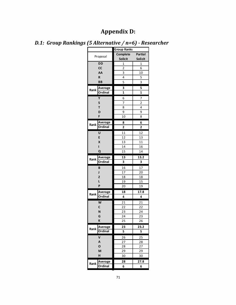
71
Appendix D:
D.1: Group Rankings (5 Alternative / n=6) - Researcher
OriginalComplete
Solicit
Partial
Solicit
DD 1 1 1CC 4 2 6
AA 6 3 10
R 11 4 5
BB 2 5 3
Average 4.8 3 5
Ordinal 1 1 1
Y 14 6 7
S 15 7 2
T 12 8 4
D 18 9 9F 3 10 8
Average 12.4 8 6Ordinal 3 2 2
U 17 11 12
E 5 12 13
X 10 13 11
I 21 14 16
Q 23 15 14
Average 15.2 13 13.2
Ordinal 4 3 3
B 9 16 17
J 8 17 20
Z 7 18 18L 20 19 15P 13 20 19
Average 11.4 18 17.8
Ordinal 2 4 4
W 16 21 21
C 19 22 22
N 25 23 24
G 22 24 23K 27 25 26
Average 21.8 23 23.2Ordinal 5 5 5
V 28 26 25A 26 27 28O 24 28 27
M 29 29 29
H 30 30 30
Average 27.4 28 27.8
Ordinal 6 6 6Rank
Proposal
Rank
Rank
Rank
Rank
Rank
Group Ranks

72
D.2: Group Rankings (5 Alternatives / n=6) – Marine Commander
Complete
Solicit
Partial
Solicit
1 1
2 2
3 6
4 3
5 4
Average 3 3.2
Ordinal 1 1
6 5
7 10
8 8
9 9
10 11
Average 8 8.6
Ordinal 2 2
11 13
12 14
13 12
14 7
15 15
Average 13 12.2
Ordinal 3 3
16 16
17 20
18 19
19 17
20 18
Average 18 18
Ordinal 4 4
21 21
22 22
23 23
24 25
25 24
Average 23 23
Ordinal 5 5
26 26
27 27
28 28
29 29
30 30
Average 28 28
Ordinal 6 6
A
M
H
W
K
O
V
N
J
L
G
I
B
E
F
Proposal
CC
P
DD
BB
Z
Rank
Rank
Rank
Rank
Rank
Rank
AA
R
Y
T
D
S
X
C
Q
U

73
D.3: Group Rankings (3 Alternatives / n=10)
OriginalComplete
Solicit
Partial
Solicit
DD 1 1 1
CC 4 2 6
AA 6 3 10
Average 3.666667 2 5.666667
Ordinal 1 1 2
R 11 4 5
BB 2 5 3
Y 14 6 7
Average 9 5 5Ordinal 4 2 1
S 15 7 2
T 12 8 4D 18 9 9
Average 15 8 5Ordinal 5 3 1
F 3 10 8
U 17 11 12E 5 12 13
Average 8.333333 11 11Ordinal 3 4 3
X 10 13 11
I 21 14 16
Q 23 15 14
Average 18 14 13.66667
Ordinal 7 5 4
B 9 16 17
J 8 17 20
Z 7 18 18
Average 8 17 18.33333
Ordinal 2 6 5
L 20 19 15
P 13 20 19W 16 21 21
Average 16.33333 20 18.33333Ordinal 6 7 5
C 19 22 22
N 25 23 24G 22 24 23
Average 22 23 23Ordinal 8 8 6
K 27 25 26
V 28 26 25
A 26 27 28
Average 27 26 26.33333
Ordinal 9 9 7
O 24 28 27
M 29 29 29
H 30 30 30
Average 27.66667 29 28.66667
Ordinal 10 10 8Rank
Proposal
Rank
Rank
Rank
Rank
Rank
Rank
Rank
Rank
Rank
Rank
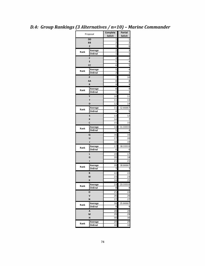
74
D.4: Group Rankings (3 Alternatives / n=10) – Marine Commander
Complete
Solicit
Partial
Solicit
1 1
2 2
3 6
Average 2 3
Ordinal 1 1
4 3
5 4
6 5
Average 5 4
Ordinal 2 2
7 10
8 8
9 9
Average 8 9
Ordinal 3 3
10 11
11 13
12 14
Average 11 12.66667
Ordinal 4 5
13 12
14 7
15 15
Average 14 11.33333
Ordinal 5 4
16 16
17 20
18 19
Average 17 18.33333
Ordinal 6 6
19 17
20 18
21 21
Average 20 18.66667
Ordinal 7 7
22 22
23 23
24 25
Average 23 23.33333
Ordinal 8 8
25 24
26 26
27 27
Average 26 25.66667
Ordinal 9 9
28 28
29 29
30 30
Average 29 29
Ordinal 10 10
Rank
Rank
Rank
Rank
Rank
Rank
A
M
H
W
K
O
V
N
J
L
G
I
B
E
F
Proposal
CC
P
Rank
Rank
DD
BB
Z
Rank
Rank
AA
R
Y
T
D
S
X
C
Q
U
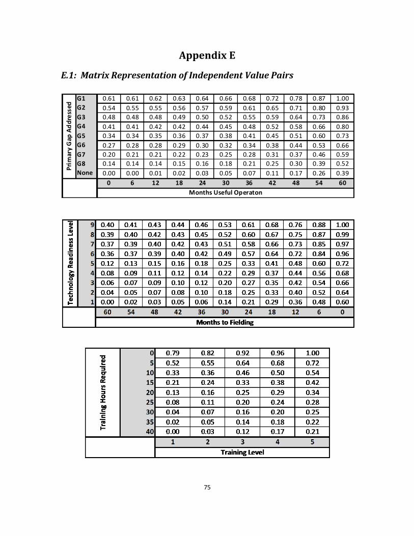
75
Appendix E
E.1: Matrix Representation of Independent Value Pairs
G1 0.61 0.61 0.62 0.63 0.64 0.66 0.68 0.72 0.78 0.87 1.00
G2 0.54 0.55 0.55 0.56 0.57 0.59 0.61 0.65 0.71 0.80 0.93
G3 0.48 0.48 0.48 0.49 0.50 0.52 0.55 0.59 0.64 0.73 0.86
G4 0.41 0.41 0.42 0.42 0.44 0.45 0.48 0.52 0.58 0.66 0.80
G5 0.34 0.34 0.35 0.36 0.37 0.38 0.41 0.45 0.51 0.60 0.73
G6 0.27 0.28 0.28 0.29 0.30 0.32 0.34 0.38 0.44 0.53 0.66
G7 0.20 0.21 0.21 0.22 0.23 0.25 0.28 0.31 0.37 0.46 0.59
G8 0.14 0.14 0.14 0.15 0.16 0.18 0.21 0.25 0.30 0.39 0.52
None 0.00 0.00 0.01 0.02 0.03 0.05 0.07 0.11 0.17 0.26 0.39
0 6 12 18 24 30 36 42 48 54 60
Pri
mar
y G
ap A
dd
ress
ed
Months Useful Operaton

76
Appendix F
F.1: Sensitivity Analysis (Needed Capability)
0
0.1
0.2
0.3
0.4
0.5
0.6
0.7
0.8
0.9
1
0 0.2 0.4 0.6 0.8 1
Sco
re
Weight
Original
0
0.1
0.2
0.3
0.4
0.5
0.6
0.7
0.8
0.9
1
0 0.2 0.4 0.6 0.8 1
Sco
re
Weight
Combined
0
0.2
0.4
0.6
0.8
1
0 0.2 0.4 0.6 0.8 1
Sco
re
Weight
CombinedMarine Commander
Researcher
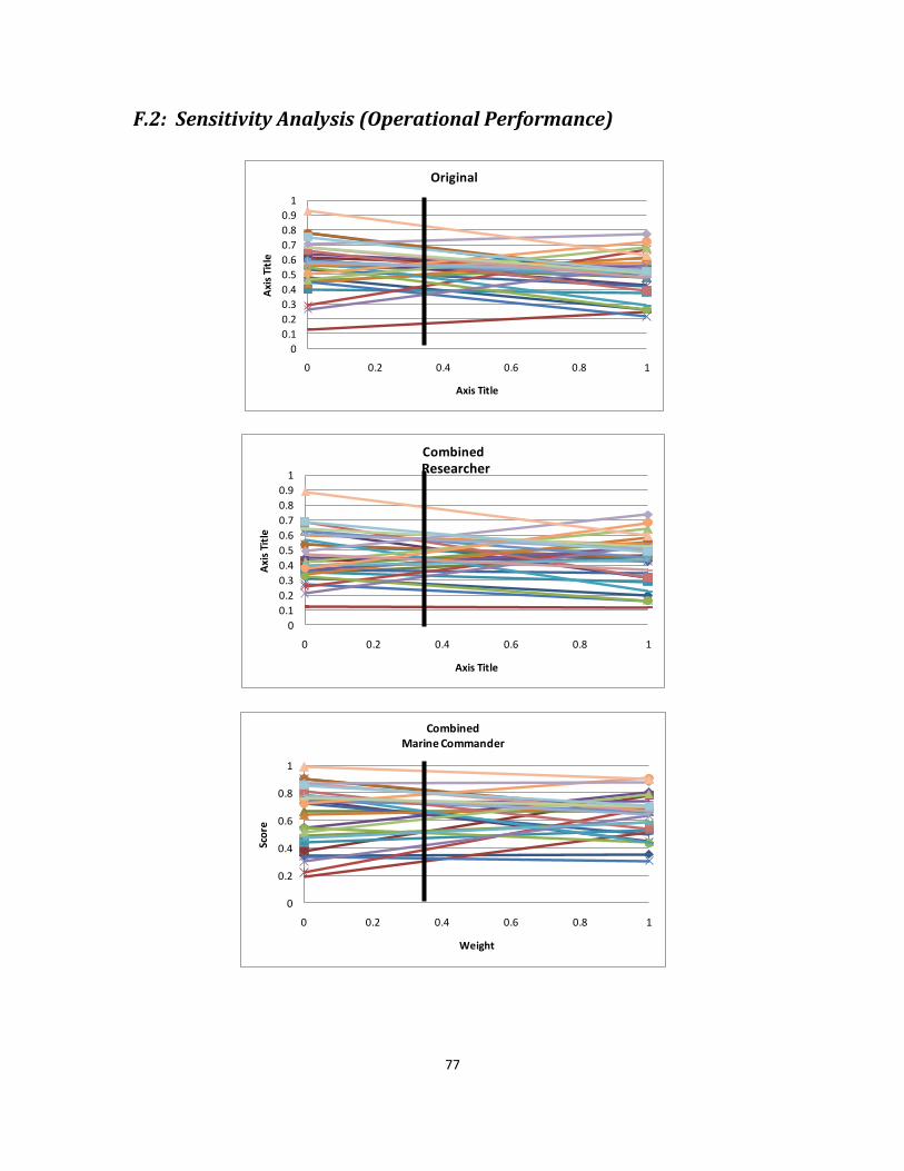
77
F.2: Sensitivity Analysis (Operational Performance)
0
0.1
0.2
0.3
0.4
0.5
0.6
0.7
0.8
0.9
1
0 0.2 0.4 0.6 0.8 1
Axi
s Ti
tle
Axis Title
Original
0
0.1
0.2
0.3
0.4
0.5
0.6
0.7
0.8
0.9
1
0 0.2 0.4 0.6 0.8 1
Axi
s Ti
tle
Axis Title
Combined
0
0.2
0.4
0.6
0.8
1
0 0.2 0.4 0.6 0.8 1
Sco
re
Weight
CombinedMarine Commander
Researcher

78
F.3: Sensitivity Analysis (Usability)
0
0.1
0.2
0.3
0.4
0.5
0.6
0.7
0.8
0.9
1
0 0.2 0.4 0.6 0.8 1
Axi
s Ti
tle
Axis Title
Original
0
0.1
0.2
0.3
0.4
0.5
0.6
0.7
0.8
0.9
1
0 0.2 0.4 0.6 0.8 1
Axi
s Ti
tle
Axis Title
Combined
0
0.2
0.4
0.6
0.8
1
0 0.2 0.4 0.6 0.8 1
Sco
re
Weight
CombinedMarine Commander
Researcher

79
Appendix G
”All Models Are Wrong…”
“… but some are useful”. George Box the famous industrial statistician
uttered those words over 30 years ago and they remain every bit as true to this day.
Over the past century modeling technology and computing power have led to an
increasing set of tools available to the analyst. Yet they are still all fundamentally
abstractions of reality and must still answer the number question of any decision maker
confronted with pages of data and analysis: “So, how does this help me?”
As resources and capital become increasingly scarce in the current
economic environment decision makers are being forced to take a closer look at what
projects and investments they pursue before committing their resources. Not only are
these choices complex but in an age of increased accountability they require a high level
of transparency and objectivity. “We felt it was best at the time” is no longer a good
enough answer.
Decision Analysis (DA) fills this gap with models designed to accurately
and consistently reflect the values of decision makers. By breaking down large decisions
into manageable and measurable pieces DA helps companies and individuals quickly and
accurately calculate tradeoffs and rank alternative sets.
With much research in the field of DA, the challenge is to balance mathematical
rigor while keeping the decision maker at the center of the model. A decision maker will

80
not use a model they do neither understand nor believe and they should not use a
model which does not accurately reflect their values.
Consider JIEDDO, the Joint Improvised Explosive Device Defeat Organization.
They are the primary government body charged with evaluating potential counter-IED
solutions and determining which proposals should be funded to maximize the impact
against the war on terror. DA provides a perfect fit to help JIEDDO filter through the
thousands of proposals and weigh them against the myriad of strengths they bring to
the fight. Like many organizations before it JIEDDO settled on a Value Focused Thinking
model due to its relative simplicity and clear requirements.
JIEDDO’s model can be thought of as thirteen people each grading a single
quality of a specific counter-IED technology. Once each of them has assigned their
variable a score, the scores for each alternative are placed in separate boxes. Finally
each alternative is ranked based on whose box has the most score.
But in JIEDDO’s case this isn’t the full story. The problem comes later when the
different evaluators get to talking. Consider a rock, submitted as a medium-range,
hand-held technology for soldiers to fight the threat of human-borne IEDs. Both raters
for “Fielding Timeline” and “Technical Risk” gave the rock full marks because it’s ready
now and because “rock” technology is definitely mature. It’s not until they find out that
the “Technical Performance” rater gave the rock a score of zero for providing virtually
none of the capability required by the mission that both the previous raters want their
score sheets back. If they’d known it performed so poorly they would have never given
it such a high score.

81
JIEDDO’s model lost usefulness because it assumes independence between
factors which doesn’t exist. It fails to capture interactions between variables and misses
the mark in reflecting some of the decision maker’s holistic evaluations of measures.
While techniques exist to handle such interactions, many of them are based on complex
equations and require more intensive and lengthy interview sessions to create such
models. Again, usefulness has been lost by implanting a process which may be more
complex than the original decision.
Researchers at the Air Force Institute of Technology have risen to this challenge
and proposed a new methodology for handling such inconsistencies in decision models.
With a small set of solicited information the model is able to mathematically generate
all possible interactions between two variables with a very low margin of error.
Furthermore, this new technique is applicable either during model creation or after.
This means that organizations like JIEDDO will be able to increase the applicability of
their existent model without having to return to square one. All models may be wrong,
but by putting more of the decision maker back into the model government
organizations like JIEDDO may never again have to explain a two thousand dollar toilet
seat to congress, and that would definitely be useful.

82
Bibliography
Angilella, S., Greco, S., Lamantia, F., & Matarazzo, B. (2004). Assessing Non-Additive
Utility For Multicritereia Decision Aid. European Journal of Operational Research , 734-
744.
Bolboaca, S.-D., & Jantschi, L. (2006). Pearson versus Spearman, Kendall's Tau
Correlation Analysis on Structure-Activity Relationships of Biologic Active Compounds.
Leonardo Journal of Sciences , 179-200.
Buede, D. M., & Bresnick, T. A. (1992). Applications of Decision Analysis to the Military
Systems Acquisition Process. Interfaces , 110-125.
Carlsson, C., & Fuller, R. (1995). Multiple Criteria Decision Making: The Case for
Interdependence. Computers & Operations Research , 251-260.
Chalmer, B. J., & Whitmore, D. G. (1986). Understanding Statistics. CRC Press.
Clemen, R. T., & Reilly, T. (2001). Making Hard Decisions. Pacific Grove: Duxbury.
Coopersmith, E., Dean, G., McVean, J., & Storaune, E. (2001, Winter). Making Decisions
in the Oil and Gas Industry. Oilfield Review , pp. 2-9.

83
Dawley, L., Lenore, M., & Long, M. (2008). Developing a Decision Model for Joint
Improvised Explosive Device Defeat Organization (JIEDDO) Proposal Selection. WPAFB:
Air Force Institute of Technology.
Department of Defense. (2006). Joint Improvised Explosive Device Defeat Organization
(JIEDDO). DODD 2000.19E. Washington DC: Department of Defense.
Dyer, J. S. (1990). Remarks on the Analytic Heirarchy Process. Management Science ,
249-258.
Ewing, P. L., Tarantino, W., & Parnell, G. S. (2006). Use of Decision Analyhsis in the Army
Base Realignment and Closure (BRAC) 2005 Military Value Analysis. Decision Analysis ,
33-49.
Figueira, J. R., Greco, S., & Slowinski, R. (2009). Building a set of additive value functions
representing a reference preorder and intensities of preference: GRIP method.
European Journal of Operational research , 460-486.
Gezeravci, A. (2008). Analyzing Individual Decision Making Versus Group Deision Making
For Altenative Selection. WPAFB: Air Force Institue of Technology.

84
Government Accountability Office. (2008). More Transparency Needed Over the
Financial and Human Capital Operations of the Joint Improvised Explosive Device Defeat
Organization. Retrieved August 10, 2008, from GAO Website:
http://www.gao.gov/highlights/d08342high.pdf
Grabisch, M. (1995). Fuzzy Integral in Multicriteria Decision Making. Fuzzy Sets and
Systems , 279-298.
Grabisch, M., Murofushi, T., & Sugeno, M. (2000). Fuzzy Measures and Integrals: Theory
and Applications. Hedelberg: Physica-Verlag.
JIEDDO. (2008). About JIEDDO. Retrieved August 2, 2008, from JIEDDO Web Site:
https://www.jieddo.dod.mil/aboutjieddo/ajhome.aspx
Keefer, D. L., & Bodily, S. E. (1983). Three-Point Approximations For Continuous Random
Variables. Management Science , 595-609.
Keeney, R. (1974). Multiplicative Utility Functions. Operations REsearch , 22.
Keeney, R. (1980). Sitting Energy Facilities. New York: Academic Press.

85
Keeney, R. (1976). Utility Independence Properties On Overlapping Attributes, Research
Memorandum. International Institute for Applied Systems Analysis .
Keeney, R. (1992). Value-Focused Thinking: A Path to Creative Decisionmaking.
Cambridge: Harvard University Press.
Kirkwood, C. W. (1992). An Overview of Methods for Applied Decision Analysis.
Interfaces , 28-39.
Kirkwood, C. W. (1997). Strategic Decision Making: Multiobjective Decision Analysis With
Spreadsheets. Belmont: Wadsworth Publishing Company.
Kirkwood, C. W., & Sarin, R. K. (1980). Preference Conditions for Multiattribute Value
Functions. Opeartions Research , 225-232.
Kleindorfer, P. R., Kunreuther, H., & Schoemaker, P. J. (1993). Decision Sciences: An
Integrative Perspective. Cambridge: Cambridge University Press.
Kusnic, M. W., & Owen, D. (1992). The Unifying Vision Process: Value Beyond Traditional
Decision Analysis in Multiple-Decision-Maker Environments. Interfaces , 150-166.

86
Lahdelma, R., Makkonen, S., & Salminen, P. (2006). Two Ways to Handle Dependent
Uncertainties in Multi-Criteria Decision Problems. Omega , 79-92.
Leskinen, P., & Kangas, J. (2005). Multi-Criteria Natural Resource Management with
Preferentially Dependent Decision Criteria. Journal of Environmental Management ,
244-251.
Marichal, J., & Roubens, M. (200). Determination of Weights of Interacting Criteria From
a Reference Set. European Journal of Operational Research , 641-650.
Meigs, M. C. (2007). Army Times Editorial Board. Retrieved August 20, 2008, from Wired
Blog:http://blog.wired.com/defense/files/
070508_m4_army_times_editorial_board_final1.pdf, Montgomery, D. C. (2005). Design
and Analysis of Experiments. Hoboken: John Wiley & Sons.
Parnell, G. S., Conley, H. W., Jackson, J. A., Lehmkuhl, L. J., & Andrew, J. M. (1998).
Foundations 2025: A Value Model for Evaluating Future Air and Space Forces.
Management Science , 1336-1350.
Pett, M. A. (1997). Nonparametric Statistics for Health Care Research: Statistics for Small
Samples and Unusual Distributions. Thousand Oaks: SAGE.

87
Rohlf, F. J., & Sokal, R. R. (1995). Statistical Tables. New York: W. H. Freeman and
Company.
Saaty, T. L. (1986). Axiomatic Foundation of the Analytic Hierarchy Process.
Management Science , 841-855.
Saaty, T. L. (1994). Highlights and Critical Points in the Theory and Application of the
Analytic Hierarchy Process. European Journal of Operational Research , 426-447.
Stewart, T. J. (1981). An Interactive Approach to Multiple Criteria Decision-Making
Bason on Statistical Inference. IEEE Transactions on Systems, Man and Cybernetics , 733-
740.
Stewart, T. J. (1984). Inferring Preferences in Multiple Criteria Decision Analysis Using a
Logistic Regression Model. Management Science , 1067-1077.
United States Air Force. (2003). Air Force Basic Doctrine AFDD 1. Washington DC: United
States Air Force.
Willy, C. (2009). Robust Sensitivity Analysis for the Joint Improvised Explosive Device
Defeat Orginization (JIEDDO) Proposal Selection Model. Wright-Patterson AFB: Air Force
Instittue of Technology.

88
Vita Captain Christopher D Richards graduated from Anacortes High School in
Anacortes, Washington. He entered undergraduate studies at the Pepperdine
University in Malibu, California where he graduated with Bachelor of Science degrees in
both Computer Science and Mathematics in April 2002. He taught high school math and
physics until receiving his commission through the Officer Training School at Maxwell
AFB, Alabama and nominated for a Regular Commission.
His first assignment was at Randolph AFB as chief analyst at HQ AF Recruiting. In
July 2008, he entered the Graduate School of Engineering and Management, Air Force
Institute of Technology. Upon graduation, he will be assigned to the Office of Aerospace
Studies at Kirtland AFB.

89
REPORT DOCUMENTATION PAGE Form Approved OMB No. 074-0188
The public reporting burden for this collection of information is estimated to average 1 hour per response, including the time for reviewing instructions, searching existing data sources, gathering and maintaining the data needed, and completing and reviewing the collection of information. Send comments regarding this burden estimate or any other aspect of the collection of information, including suggestions for reducing this burden to Department of Defense, Washington Headquarters Services, Directorate for Information Operations and Reports (0704-0188), 1215 Jefferson Davis Highway, Suite 1204, Arlington, VA 22202-4302. Respondents should be aware that notwithstanding any other provision of law, no person shall be subject to an penalty for failing to comply with a collection of information if it does not display a currently valid OMB control number.
PLEASE DO NOT RETURN YOUR FORM TO THE ABOVE ADDRESS.
1. REPORT DATE (DD-MM-YYYY)
01-09-2007 2. REPORT TYPE
Master’s Thesis
3. DATES COVERED (From – To)
Jun 2008 – Mar 2009
4. TITLE AND SUBTITLE
CREATING MULTI OBJECTIVE VALUE FUNCTIONS FROM NON-
INDEPENDENT VALUES
5a. CONTRACT NUMBER
5b. GRANT NUMBER
5c. PROGRAM ELEMENT NUMBER JON 09254
6. AUTHOR(S)
Richards, Christopher D., Capt, USAF
5d. PROJECT NUMBER 1.B
5e. TASK NUMBER
5f. WORK UNIT NUMBER
7. PERFORMING ORGANIZATION NAMES(S) AND ADDRESS(S)
Air Force Institute of Technology
Graduate School of Engineering and Management (AFIT/EN)
2950 Hobson Street, Building 642
WPAFB OH 45433-7765
8. PERFORMING ORGANIZATION REPORT NUMBER
AFIT/GOR/ENS/09-12
9. SPONSORING/MONITORING AGENCY NAME(S) AND ADDRESS(ES)
Dr. Seth Howell Joint Improvised Explosive Device Defeat Organization (JIEDDO) 2521 South Clark Street Arlington, VA 22202
10. SPONSOR/MONITOR’S ACRONYM(S)
11. SPONSOR/MONITOR’S REPORT NUMBER(S)
12. DISTRIBUTION/AVAILABILITY STATEMENT APPROVED FOR PUBLIC RELEASE; DISTRIBUTION UNLIMITED.
13. SUPPLEMENTARY NOTES
14. ABSTRACT
Decisions are made every day and by everyone. As these decisions become more important, involve higher costs and affect a broader group of
stakeholders it becomes essential to establish a more rigorous strategy than simply intuition or “going with your gut”. In the past several decades,
the concept of Value Focused Thinking (VFT) has gained much acclaim in assisting Decision Makers (DMs) in this very effort. By identifying and
organizing what a DM values VFT is able to decompose the original problem and create a mathematical model to score and rank alternatives to be
chosen. But what if the decision should not be completely decomposed? What if there are factors that are inextricably linked rather than
independent? In the past several years, Improvised Explosive Devices (IEDs) have quickly become the number one killer of American troops
overseas. To this end the Joint IED Defeat Organization worked to create a VFT model to solicit and grade countermeasure proposals as candidates
for funding. While much time and care was put into soliciting a valid VFT hierarchy from the appropriate DM, it does not represent the only option.
With JIEDDO as an example this paper examines a strategy to better reflect a DM’s combined values in a way which is understandable to the DM
and maintains a level of mathematical rigor.
15. SUBJECT TERMS
Joint Improvised Explosive Device Defeat Organization (JIEDDO), Value Focused Thinking (VFT), Preferential Independence,
Single Dimensional Value Function (SDVF), Cross Terms, Multi Dimensional Value Function, Decision Analysis (DA), Interaction,
Linear Interpolation
16. SECURITY CLASSIFICATION OF: 17. LIMITATION OF ABSTRACT
UU
18. NUMBER OF PAGES
99
19a. NAME OF RESPONSIBLE PERSON Jeffery Weir, PhD (ENS)
a. REPORT
U
b. ABSTRACT
U
c. THIS PAGE
U
19b. TELEPHONE NUMBER (Include area code) (937) 257-6531 e-mail: [email protected]
Standard Form 298 (Rev. 8-98) Prescribed by ANSI Std. Z39-18