creating bi solutions with bism tabular

Written By: Dan Clark

Creating BI solutions with BISM Tabular

INTRODUCTION

PAGE 4 SSAS TABULAR MODE

PAGE 5 TABULAR MODELING

PAGE 7 CREATING A TABULAR MODEL

PAGE 8 IMPORTING DATA

PAGE 9 CREATING RELATIONSHIPS

PAGE 9 CREATING CALCULATED COLUMNS, MEASURES AND KPIS

PAGE 1 1 SECURITY

PAGE 1 2 TESTING THE TABULAR MODEL

PAGE 13 DEPLOYING A TABULAR MODEL

PAGE 14 CONNECTING TO A TABULAR MODEL

PAGE 17 SUMMARY

CONTENTS

PRAGMATIC WORKS White Paper Creating BI solutions with BISM Tabular

www.pragmaticworks.com PAGE 3

INTRODUCTION

Business Intelligence, the process of analyzing business data

to support better decision making, has become a necessity for

most businesses in today’s competitive environment. In order to

bring BI to small and mid-sized companies, there needs to be a

set of affordable easy to use tools at their disposal. Microsoft

has long had a vision and commitment to bringing the power of

BI to the masses, and creating a set of tools and technologies to

allow for self-service BI.

One of the major hurdles of bringing BI to the masses is the

complexity of developing data warehouse models using the

OLAP processing engine in SQL Server Analysis Services (SSAS).

Add to this the complexity of querying the data with MDX and

you have a challenging road block for most small to medium

sized organizations. In order to help overcome these hurdles,

Microsoft has introduced the Business Intelligence Semantic

Model (BISM). BISM supports two models, the traditional

multidimensional model and a new tabular model. The tabular

model is based on a relational table model which is familiar to

DBA’s, developers, and power users. In addition, Microsoft has

created a new query language to query the BISM Tabular model.

This language, Data Analysis Expression Language (DAX), is

similar to the syntax used in Excel calculations and should be

familiar to the Excel power users.

The goal of this white paper is to expose you to the process

needed to create a BISM Tabular Model in SQL Server 2012 and

deploy it to an Analysis Server where it can be exposed to client

applications. This is not an in depth discussion of the process but

rather an overview of the methods involved.



SSAS TABULAR MODE

SSAS supports both traditional multidimensional models using

the MOLAP storage engine and tabular models using the new

Vertipaq engine. However, the same instance of SSAS cannot

support both types of projects. If you need to support both

multidimensional and tabular projects you must install a separate

instance for each.

While the traditional MOLAP engine is optimized for OLAP

using techniques such as pre-built aggregates, bitmap indexes,

and compression to deliver great performance and scale, the

Vertipaq engine takes a different approach. Vertipaq is an in-

memory column store engine that combines data compression

and scanning algorithms to deliver fast performance with no

need for indexes or pre-built aggregation. In addition, since all

aggregation occurs on the fly in memory, it avoids costly I/O reads

to disk storage.

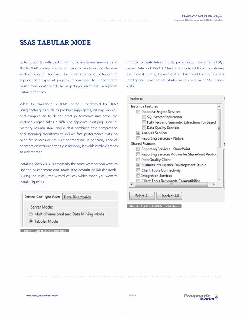
Installing SSAS 2012 is essentially the same whether you want to

use the Multidemensional mode (the default) or Tabular mode.

During the install, the wizard will ask which mode you want to

install (Figure 1).

Figure 1 – Choosing SSAS Tabular Mode

Figure 2 – Installing the SQL Server Data Tools

In order to create tabular model projects you need to install SQL

Server Data Tools (SSDT). Make sure you select this option during

the install (Figure 2). Be aware, it still has the old name, Business

Intelligence Development Studio, in this version of SQL Server

2012.



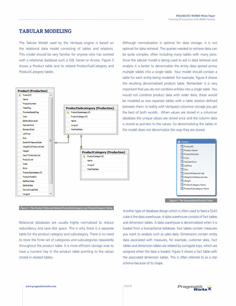
Although normalization is optimal for data storage, it is not

optimal for data retrieval. The queries needed to retrieve data can

be quite complex, often including many tables with many joins.

Since the tabular model is being used to aid in data retrieval and

analysis it is better to denormalize the entity data spread across

multiple tables into a single table. Your model should contain a

table for each entity being modeled. For example, figure 4 shows

the resulting denormalized product table. Remember it is very

important that you do not combine entities into a single table. You

would not combine product data with order data; these would

be modeled as two separate tables with a table relation defined

between them. In reality with Vertipaq’s columnar storage you get

the best of both worlds. When values are stored in a columnar

database the unique values are stored once and the column data

is stored as pointers to the values. So denormalizing the tables in

the model does not denormalize the way they are stored.

TABULAR MODELING

The Tabular Model used by the Vertipaq engine is based on

the relational data model consisting of tables and relations.

This model should be very familiar for anyone who has worked

with a relational database such a SQL Server or Access. Figure 3

shows a Product table and its related ProductSubCategory and

ProductCategory tables.

Figure 3 - The Product Table and Related ProductSubCategory and ProductCategory Tables

Figure 4 - The Denormalized Product Table

Relational databases are usually highly normalized to reduce

redundancy and save disk space. This is why there is a separate

table for the product category and subcategory. There is no need

to store the finite set of categories and subcategories repeatedly

throughout the product table. It is more efficient storage wise to

have a numeric key in the product table pointing to the values

stored in related tables.

Another type of database design which is often used to feed a SSAS

cube is the data warehouse. A data warehouse consists of fact tables

and dimension tables. A data warehouse is denormalized when it is

loaded from a transactional database. Fact tables contain measures

you want to analyze such as sales data. Dimensions contain entity

data associated with measures, for example, customer data. Fact

tables and dimension tables are related by surrogate keys, which are

assigned when the data is loaded. Figure 5 shows a fact table with

the associated dimension tables. This is often referred to as a star

schema because of its shape.



Figure 5 – Typical star schema in a data warehouse

Figure 6 – Creating a Tabular Project

A data warehouse containing star schemas

makes an excellent data sources for a tabular

model. They are already denormalized and

contain clearly defined relationships. Although

you could pull data from the Analysis Service

OLAP cube that the data warehouse feeds,

you have to use MDX and complex queries to

retrieve and flatten the data. You in essence

must reverse engineer the OLAP cube back into

the relational star schema.



CREATING A TABULAR MODEL

In order to create a tabular model project, you need to launch an instance of SQL Server

Data Tools. In the New Project dialog box, under Installed Templates, you select the Business

Intelligence templates. Under the Analysis Services templates, you should see the Analysis

Services Tabular Project template (Figure 6).



IMPORTING DATA

When you import data into a tabular model, you are loading a copy

of the data into a column-store. A column-store maintains the data

in separate columns instead of the traditional row based storage,

which keeps the rows together. In column based storage a high

degree of compression is achieved when columns contain redundant

data such as dates or gender. The column-store only has to store the

discrete values once and then create pointers to the values. Column-

stores also have the advantage of faster queries because there is

no need to access entire rows from the database, just the columns

needed for the query. These attributes make column storage ideal

for ad-hoc reporting and data analysis applications.

You can import data into a tabular model project from a variety of

sources including relational databases, multidimensional cubes,

text files, and data feeds. The Table Import Wizard guides you

through the steps necessary to import the data. First you choose a

data source and create a connection. The connection information

required is determined by the type of connection used. Figure 7

shows the dialog for connecting to a SQL Server database.

Figure 7 – Connecting to a SQL Server Database

Figure 8 – Choosing Tables to Import

Figure 9 – Creating Your Own Data Import Queries

After entering security credentials you get the option of selecting

data from a list of tables and views or entering a query to select

the data. By selecting the tables and views option, you can select

tables to import, automatically select related tables, and provide

filters for the data import (Figure 8).

Selecting the query option allows you to create your own queries

to retrieve data from tables, views, or stored procedures (Figure

9). You can also launch a pretty handy query designer to help

construct your queries.



CREATING RELATIONSHIPS

CREATING CALCULATED COLUMNS, MEASURES AND KPIS

Once you have imported the data it’s time to create relationships

between the tables. When you import data from a relational

database system, the Data Import Wizard will detect relationships

defined in the database and automatically import them for you.

There are two views you can use to examine the model, the Data

View and the Diagram View. Viewing the model in the Diagram

View mode reveals the relationships between the tables (Figure 10).

Figure 10 – Diagram View Mode

Figure 11 – Data View Mode

Figure 12 – Creating a Calculated Column in the Formula Bar

To edit a relationship, you just double-click on the relationship

arrow, which launches the Edit Relationship dialog. To create

a new relationship you can drag and drop the related field

from one table to the other. For example, drag and drop the

ProductCategoryKey from the ProductCategory table to the

ProductCategoryKey in the ProductSubcategory table.

In order to create calculated columns and measures in a BISM

Tabular model you use the Data Analysis Expression language

(DAX). If you have ever worked with formulas in excel, you will

find the DAX language syntax very familiar. DAX works with the

Vertipaq engine to quickly perform calculations on large volumes

of in-memory data.

Calculated columns are columns you add to an existing table in

the tabular model. The value of the column is calculated for each

row at the time you create the column. It is recalculated if the

underlying data is refreshed. These values are static values that do

not change as the client slices the data in a PivotTable.

To create a calculated column in the tabular model, change the

model designer so that it is in the Data View Mode. The Data

View mode shows the data in an Excel-like sheet, with each table

as a separate tab (Figure 11).

To create a calculated column, right click on any column and select

insert column. At the top of the sheet is the formula bar where

you enter the formula for the calculated column. For example,

Figure 12 shows a margin calculated column in the sales table.



Unlike a calculated column a measure is a calculation based

on the set of data being evaluated. They are often based on

aggregate functions such as count and sum. For example a client

application may request the total sales amount for each country

by year. Since the value in each cell of the PivotTable is dependent

on the combination of row and column headers, the formula

needs to be evaluated for each cell. As the user applies different

filters, the values are dynamically recalculated for the cells. The

Vertipaq engine is designed to provide optimum performance,

through its use of column storage and in memory data storage,

when calculating measures on the fly.

To create a measure, you use the measure grid at the bottom of

the table. You simply click on an empty cell in the measure grid

and type the formula in the formula bar. Figure 13 shows a Total

Units measure that sums up the total units sold.

Figure 13 – Creating a Measure Using the Formula Bar

Figure 14 – Creating a KPI

Figure 15 – Setting up Threshold ValuesKey Performance Indicators (KPIs) are often used to gauge

performance and identify trends. For example, you may want

to measure sales against a target sales value. A KPI calculation

includes a base value, target value, and a status threshold. The

base value is the measure you are interested in analyzing, for

example, the sales amount. The target value is the goal and

you are comparing the base value to this goal, for example,

sales quota. The status threshold defines how the comparison is

interpreted and is often used with a graphic (red, yellow, green)

to help users quickly determine performance.

To create a KPI, right-click on the measure you want to use for

the base value and select Create KPI. This launches the Key

Performance Indicator dialog. Figure 14 shows a KPI created

using the Sales as the base value and the Sales Quota as the

target value.

The next step in creating a KPI is to set the threshold values and

choose an image to display for the values. Figure 15 shows the

threshold values for the Sales KPI.

For more information on DAX refer to the whitepaper “Data

Analysis Expressions (DAX) In the Tabular BI Semantic Model”

available for download at

http://go.microsoft.com/fwlink/?LinkID=237472&clcid=0x409.



Figure 16 – Setting up Role base Security

Figure 17 – Implementing Row Level Security

SECURITY

Security in a tabular model is based on roles and permissions. You

create a role and assign permissions to the role. These permissions

define the actions that a role member can take and what data

they can see. Windows users and groups are assigned to the

roles. A user can belong to more than one role and permissions

are cumulative by least restrictive. For example, if a user belongs

to one role with read permissions and another role with the

Read and Process permission, the Read and Process permission is

used. The Role Manager dialog is used to add roles to the Tabular

Model (Figure 16).

You can also implement row level security using a DAX expression

that evaluates to true or false. For example in Figure 17, the role

is restricted to the US data.

If you need to implement dynamic security (security based on

user name instead of a role), you can use the DAX UserName

function which returns the domain\username of the currently

logged on user. You can then use this information to look up

pertinent data such as department Id and restrict row access by

department.



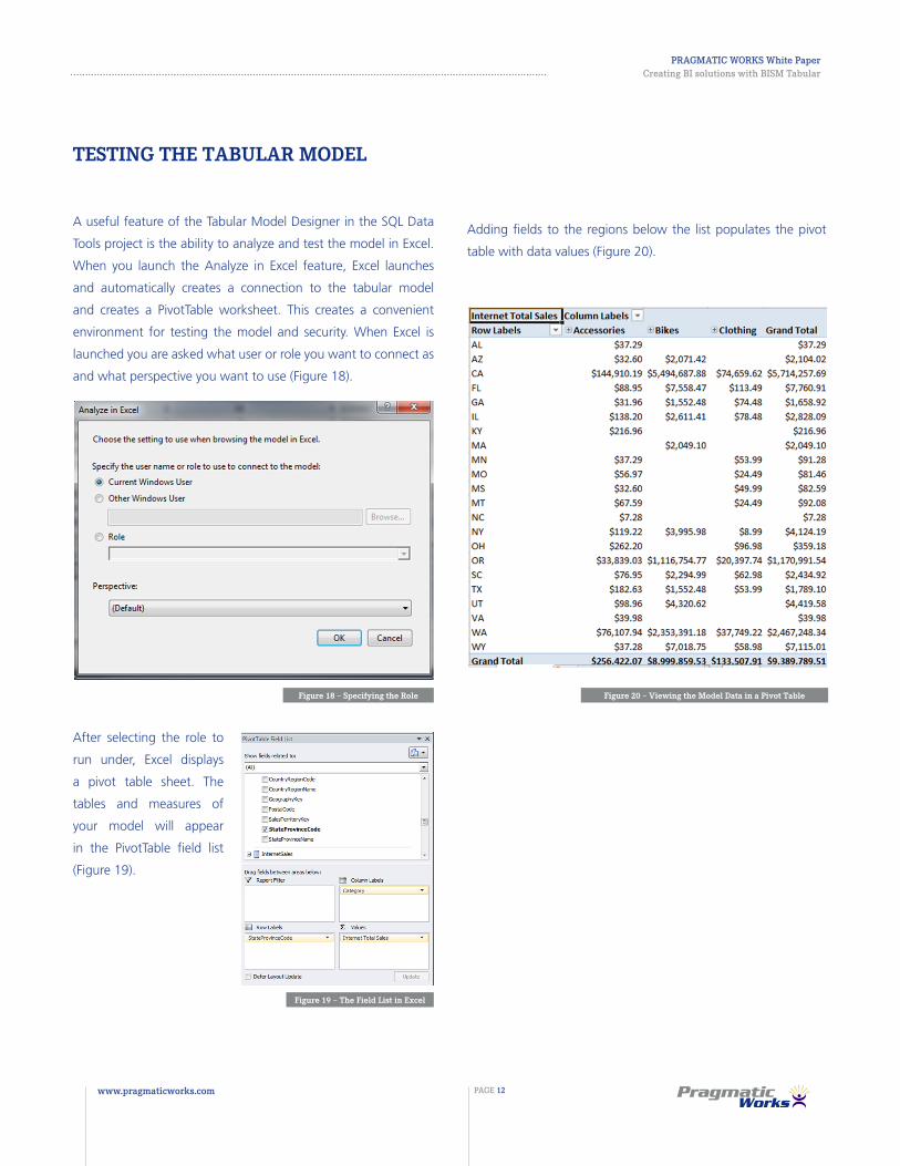
TESTING THE TABULAR MODEL

A useful feature of the Tabular Model Designer in the SQL Data

Tools project is the ability to analyze and test the model in Excel.

When you launch the Analyze in Excel feature, Excel launches

and automatically creates a connection to the tabular model

and creates a PivotTable worksheet. This creates a convenient

environment for testing the model and security. When Excel is

launched you are asked what user or role you want to connect as

and what perspective you want to use (Figure 18).

Figure 18 – Specifying the Role Figure 20 – Viewing the Model Data in a Pivot Table

Figure 19 – The Field List in Excel

After selecting the role to

run under, Excel displays

a pivot table sheet. The

tables and measures of

your model will appear

in the PivotTable field list

(Figure 19).

Adding fields to the regions below the list populates the pivot

table with data values (Figure 20).

Figure 20 – Setting Deployment Options

Figure 22 – Viewing the Tabular Model in SSAS

After you create and test a tabular model, it has to be deployed

to a SSAS server running in tabular mode. Once the solution is

deployed users can browse the model using a client application

such as a Reporting Services report, Power View (Hosted in

SharePoint 2010), or Excel.

The project deployment options, which you can open by right

clicking on the project and selecting properties, determine where

the project gets deployed and whether it should be processed

(Figure 21). You can set options for your test, staging, and

production environments depending on your deployment rules.

Once these properties are set you can right-click on the project

node in the Solution Explorer and select Deploy.

There are a number of ways you can deploy a model from

one Analysis Server to another, for example, from a staging

environment to a production environment. Among the most

popular are XMLA script, the Deployment Wizard, the Synchronize

Database Wizard, and Backup and Restore. (For more information

on deployment see: http://msdn.microsoft.com/en-us/library/

gg492138(v=sql.110).aspx )Figure 22 shows a tabular model

deployed to an Analysis Server.



DEPLOYING A TABULAR MODEL

The most common client applications connecting to a tabular

model are Excel, SSRS 2012 Reports, Power View (Hosted in

SharePoint 2010) and PerformancePoint dashboards. Although I

am not going to go into great detail about these applications, I do

want to show you how easy it is to connect to a tabular model.

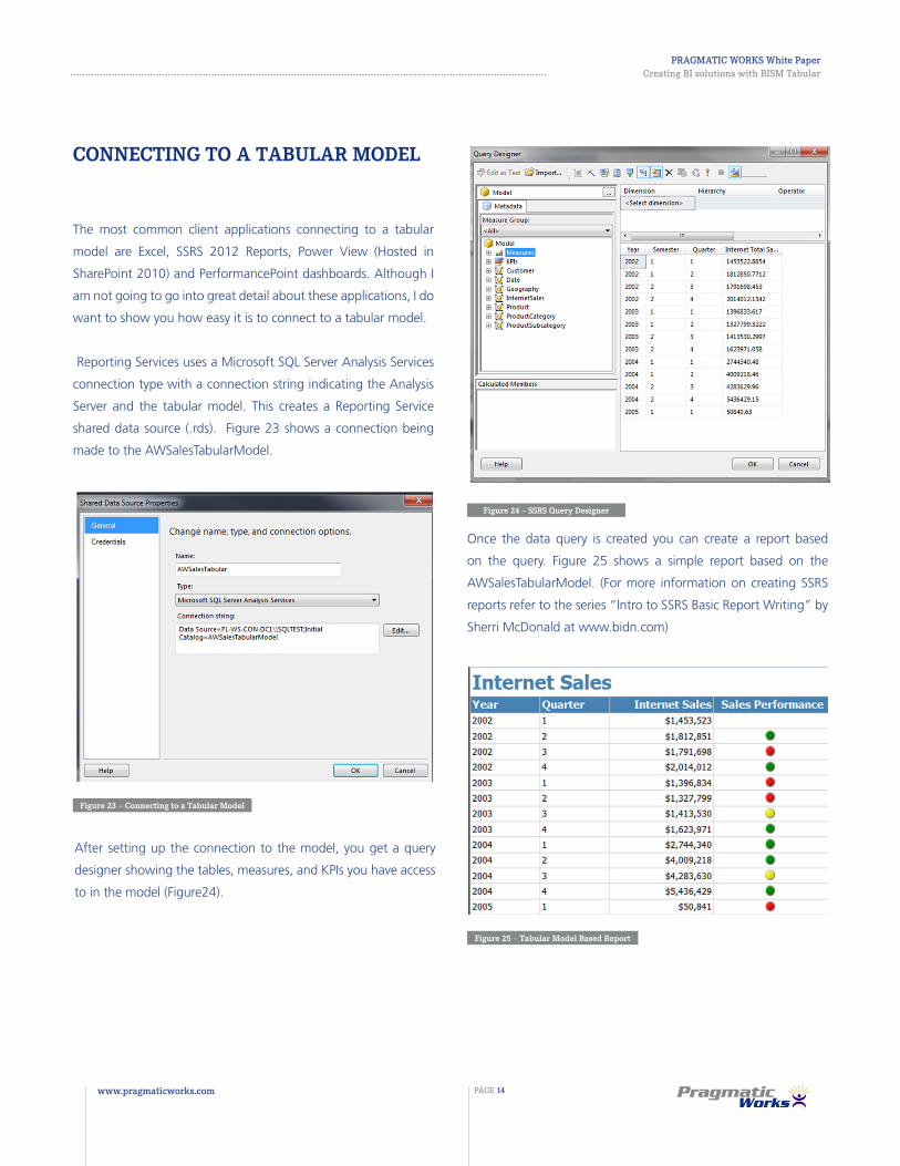
Reporting Services uses a Microsoft SQL Server Analysis Services

connection type with a connection string indicating the Analysis

Server and the tabular model. This creates a Reporting Service

shared data source (.rds). Figure 23 shows a connection being

made to the AWSalesTabularModel.

Figure 23 – Connecting to a Tabular Model

Figure 24 – SSRS Query Designer

Figure 25 – Tabular Model Based Report

After setting up the connection to the model, you get a query

designer showing the tables, measures, and KPIs you have access

to in the model (Figure24).

Once the data query is created you can create a report based

on the query. Figure 25 shows a simple report based on the

AWSalesTabularModel. (For more information on creating SSRS

reports refer to the series “Intro to SSRS Basic Report Writing” by

Sherri McDonald at www.bidn.com)



CONNECTING TO A TABULAR MODEL

To connect to the tabular model in Excel you set up an Office Data

Connection as shown in Figure 26.

Figure 26 – Creating an Office Data Connection to the Tabular Model

Figure 27 - Setting up a BI Semantic Connection in SharePoint

Figure 28 – The Power View Designer

Once this connection is made, you can explore the model using

an Excel pivot table.

Power View is a SSRS 2012 add-in for SharePoint 2010 providing

an interactive experience for the end user. It can use a SharePoint

Reporting Service shared data source (.rsds) or a BI semantic

connection (.bism) hosted in SharePoint. The SharePoint

Reporting Service shared data source is the same as the Reporting

Service shared data source (.rds) created in Reporting Services just

in a slightly different format. Setting up a BI semantic connection

in SharePoint is shown in Figure 27.

Once the BI semantic connection is made, an interactive Power

View can be created using the connection. Figure 28 shows the

Power View design window. (For more information on Power

View see the tutorial “Create a Sample Report in Power View on

the Microsoft TechNet Wiki http://technet.microsoft.com/en-us/

default.aspx)



Another popular client application for creating and deploying

Dashboards containing KPIs, Scorecards, and reports is

PerformancePoint Services 2010. This is another service hosted

in SharePoint 2010. By creating a data source that points to

the BISM Tabular Model hosted on SSAS, you can develop

dashboards based on the Tabular Model. Figure 29 shows a

sample dashboard from the webinar “Zero to Dashboard – Intro

to PerformancePoint” available at www.pragmaticworks.com.

Figure-29 PerformancePoint 2010 Dashboard



SUMMARY

This white paper has introduced you to the BISM Tabular model. The tabular model is based on a relational table model which is more

familiar to DBA’s, developers, and power users. The tabular model forms the foundation of Microsoft’s self-service BI initiative and if you

are charged with providing a BI environment to business users, it is imperative that you understand how these technologies work and fit

together. You should now have a better understanding of the process needed to create a BISM Tabular Model and deploy it to an Analysis

Server where it can be exposed to client applications.



creating bi solutions with bism tabular

Documents